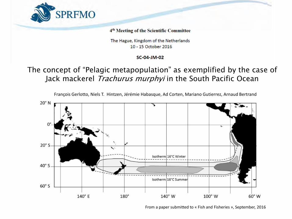
François Gerlotto, Niels T. Hintzen, Jérémie Habasque, Ad Corten, Mariano Gutierrez, Arnaud Bertrand

The concept of “Pelagic metapopulation” as exemplified by the case of Jack mackerel Trachurus murphyi in the South Pacific Ocean

From a paper submitted to « Fish and Fisheries », September, 2016

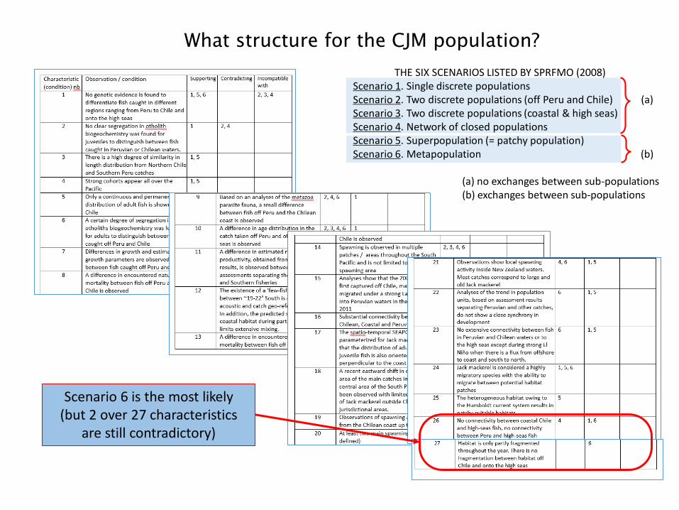
THE SIX SCENARIOS LISTED BY SPRFMO (2008)Scenario 1. Single discrete populations Scenario 2. Two discrete populations (off Peru and Chile) (a)Scenario 3. Two discrete populations (coastal & high seas)Scenario 4. Network of closed populations Scenario 5. Superpopulation (= patchy population)Scenario 6. Metapopulation (b)

(a) no exchanges between sub-populations(b) exchanges between sub-populations

Scenario 6 is the most likely(but 2 over 27 characteristics

are still contradictory)

What structure for the CJM population?

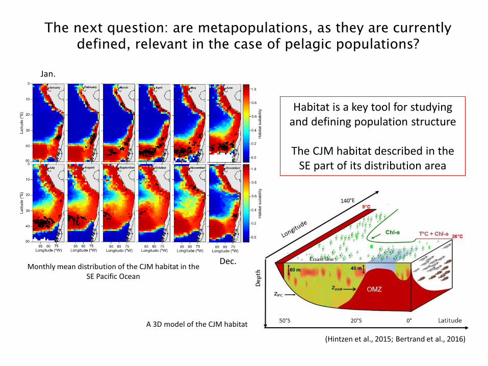
The next question: are metapopulations, as they are currentlydefined, relevant in the case of pelagic populations?

(Hintzen et al., 2015; Bertrand et al., 2016)

Monthly mean distribution of the CJM habitat in theSE Pacific Ocean

Jan.

Dec.

A 3D model of the CJM habitat

Habitat is a key tool for studyingand defining population structure

The CJM habitat described in theSE part of its distribution area

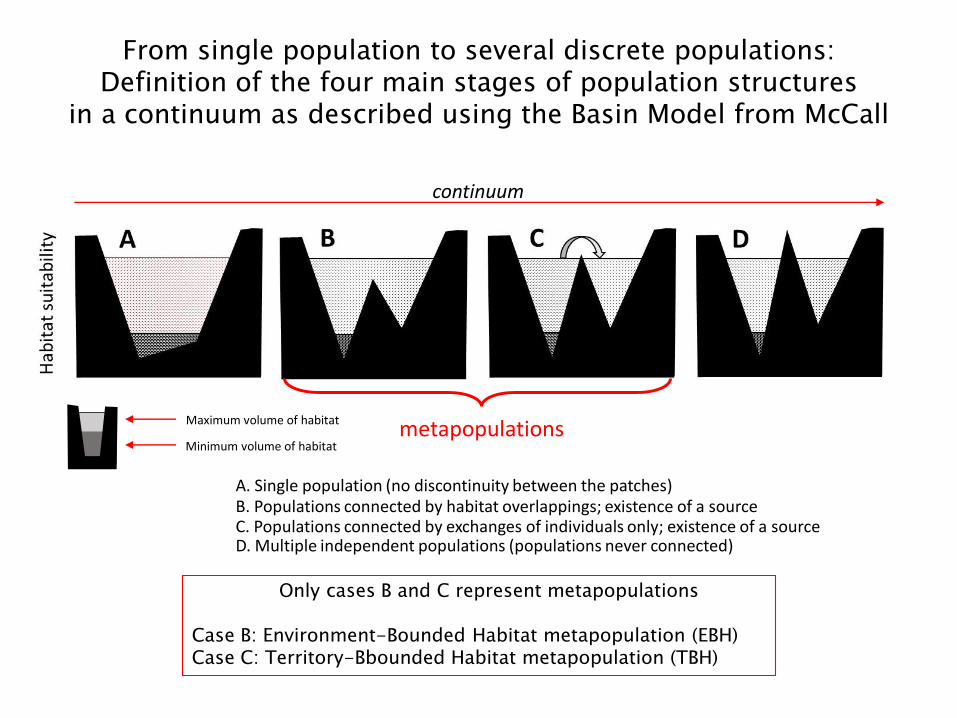
D. Multiple independent populations (populations never connected)

Maximum volume of habitat

Minimum volume of habitat

Only cases B and C represent metapopulations

Case B: Environment-Bounded Habitat metapopulation (EBH)Case C: Territory-Bbounded Habitat metapopulation (TBH)

continuum

A. Single population (no discontinuity between the patches)B. Populations connected by habitat overlappings; existence of a sourceC. Populations connected by exchanges of individuals only; existence of a source

From single population to several discrete populations:Definition of the four main stages of population structures

in a continuum as described using the Basin Model from McCall

metapopulations

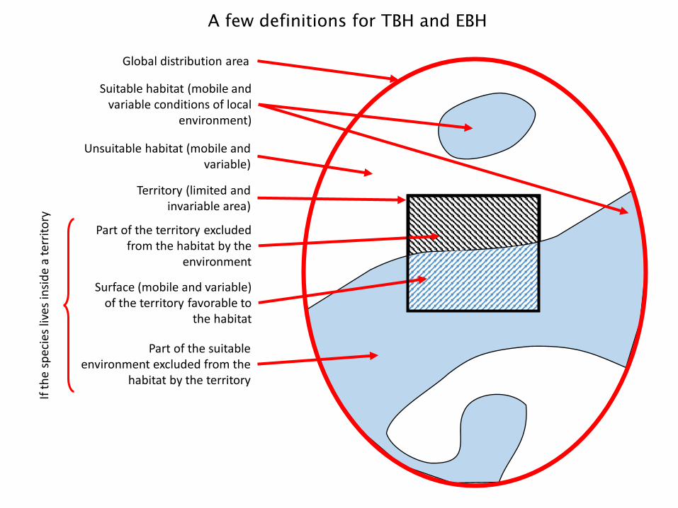
Global distribution area

Suitable habitat (mobile and variable conditions of local

environment)

Part of the territory excludedfrom the habitat by the

environment

Part of the suitableenvironment excluded from the

habitat by the territory

Surface (mobile and variable) of the territory favorable to

the habitat

Territory (limited and invariable area)

Ifth

esp

eci

esliv

esin

sid

ea

terr

ito

ry

A few definitions for TBH and EBH

Unsuitable habitat (mobile and variable)

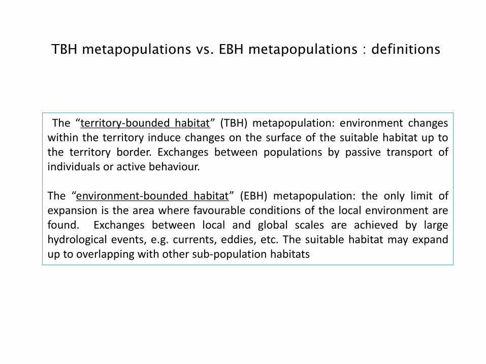
The “territory-bounded habitat” (TBH) metapopulation: environment changeswithin the territory induce changes on the surface of the suitable habitat up tothe territory border. Exchanges between populations by passive transport ofindividuals or active behaviour.

The “environment-bounded habitat” (EBH) metapopulation: the only limit ofexpansion is the area where favourable conditions of the local environment arefound. Exchanges between local and global scales are achieved by largehydrological events, e.g. currents, eddies, etc. The suitable habitat may expandup to overlapping with other sub-population habitats

TBH metapopulations vs. EBH metapopulations : definitions

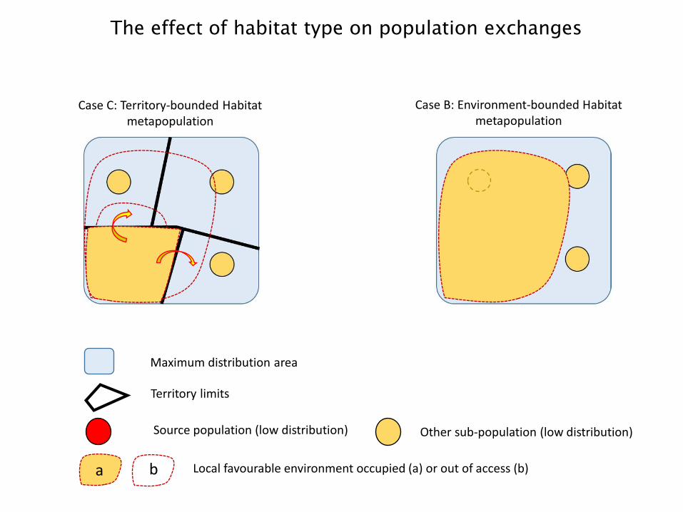
Case C: Territory-bounded Habitatmetapopulation

Case B: Environment-bounded Habitatmetapopulation

Source population (low distribution) Other sub-population (low distribution)

Local favourable environment occupied (a) or out of access (b)a b

Territory limits

Maximum distribution area

The effect of habitat type on population exchanges

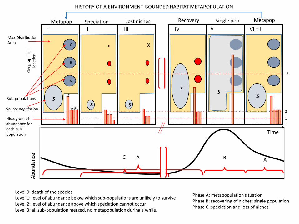
Metapop

Source population

S

0

1

2

3

IG

eogr

aph

ical

loca

tio

nMax.DistributionArea

Speciation

S

II

S

Recovery

IV

Lost niches

X

S

III

Metapop

S

VI = I

Single pop.

S

V

}AC B

Ab

un

dan

ce

A

HISTORY OF A ENVIRONMENT-BOUNDED HABITAT METAPOPULATION

Sub-populations

Histogram of abundance foreach sub-population Time

A

A

B

B C

C

S

Phase A: metapopulation situationPhase B: recovering of niches; single populationPhase C: speciation and loss of niches

Level 0: death of the speciesLevel 1: level of abundance below which sub-populations are unlikely to surviveLevel 2: level of abundance above which speciation cannot occurLevel 3: all sub-population merged, no metapopulation during a while.

Source population

0

1

2

3

Geo

grap

hic

allo

cati

on

Max.DistributionArea

} AC

Ab

un

dan

ce

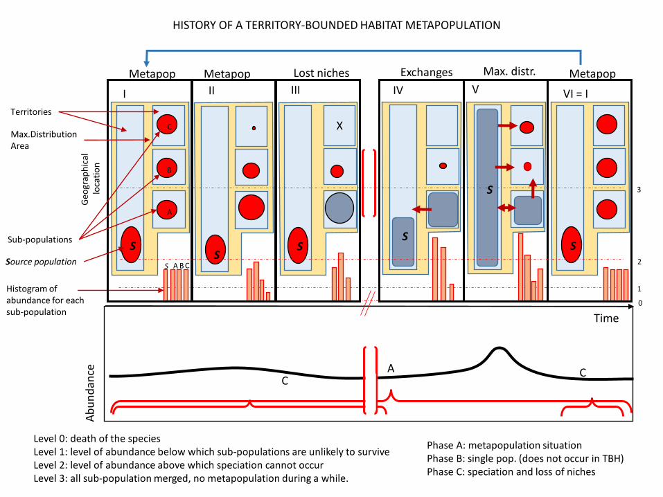
HISTORY OF A TERRITORY-BOUNDED HABITAT METAPOPULATION

Sub-populations

Histogram of abundance for eachsub-population

Time

Metapop

I

A B CS

C

B

A

S

Metapop

VI = I

S

Metapop

II

SS

Lost niches

X

III

S

X

Exchanges

IV

S

Max. distr.

V

S

C

Territories

Phase A: metapopulation situationPhase B: single pop. (does not occur in TBH)Phase C: speciation and loss of niches

Level 0: death of the speciesLevel 1: level of abundance below which sub-populations are unlikely to surviveLevel 2: level of abundance above which speciation cannot occurLevel 3: all sub-population merged, no metapopulation during a while.

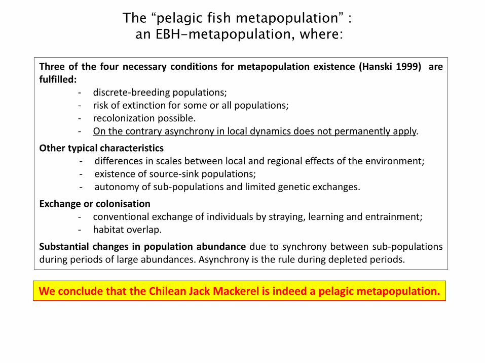
Three of the four necessary conditions for metapopulation existence (Hanski 1999) arefulfilled:

- discrete-breeding populations;- risk of extinction for some or all populations;- recolonization possible.- On the contrary asynchrony in local dynamics does not permanently apply.

Other typical characteristics- differences in scales between local and regional effects of the environment;- existence of source-sink populations;- autonomy of sub-populations and limited genetic exchanges.

Exchange or colonisation- conventional exchange of individuals by straying, learning and entrainment;- habitat overlap.

Substantial changes in population abundance due to synchrony between sub-populationsduring periods of large abundances. Asynchrony is the rule during depleted periods.

The “pelagic fish metapopulation” : an EBH-metapopulation, where:

We conclude that the Chilean Jack Mackerel is indeed a pelagic metapopulation.

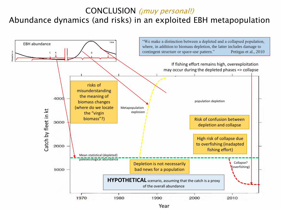
Mean statistical (depleted) paleoecological abundance

HYPOTHETICAL scenario, assuming that the catch is a proxy

of the overall abundance

Metapopulation explosion

CONCLUSION (¡muy personal!)

Abundance dynamics (and risks) in an exploited EBH metapopulation

EBH abundance

risks of misunderstanding

the meaning of biomass changes

(where do we locatethe “virginbiomass”?)

Depletion is not necessarilybad news for a population

Metapopulation depletion

“We make a distinction between a depleted and a collapsed population,

where, in addition to biomass depletion, the latter includes damage to

contingent structure or space-use pattern.” Petitgas et al., 2010

If fishing effort remains high, overexploitationmay occur during the depleted phases => collapse

Collapse? (overfishing)

High risk of collapse dueto overfishing (inadapted

fishing effort)

Risk of confusion betweendepletion and collapse