The Conduction Velocity of Intact and Regenerated Earthworms

Harnsowl Ko

Joshua Mayourian

The Cooper Union

Introduction to Neuroscience

EID330

Professor Williams

May 17th, 2013

Table of Contents Abstract.................................................................................................................................i

Introduction..........................................................................................................................1

Procedure.............................................................................................................................4

Results and Discussion........................................................................................................7

Conclusion.........................................................................................................................16

References..........................................................................................................................17

Appendix I.........................................................................................................................18

i

Abstract:

Regenerative therapy is one of many techniques used to combat disease in

neuroscience and cardiology. To improve regenerative therapeutics, it is necessary to

better understand the mechanisms and physiological effects of natural blastema

regeneration. Therefore, the conduction velocity of an earthworm animal model was

studied to crudely understand the physiological effects of natural blastema regeneration.

Specifically, electrophysiological recordings were generated on both intact and

regenerated anesthetized earthworms via PicoScope and PicoLog. The conduction

velocity of intact and regenerated earthworms was calculated as 18.9 m/s ± 9.0 m/s and

15.5 m/s ± 6.2 m/s, respectively. These results indicate no significant difference can be

drawn on intact and regenerated earthworm conduction velocities. It was also noted that

the magnitude of action potentials increased following regeneration, which was not

expected. Therefore, the mechanism resulting in a greater action potential magnitude will

be examined in the future. The use of an effective procedure to investigate the

electrophysiological properties of intact and regenerated earthworm gives potential to

also investigate other earthworm electrical properties in the future.

1

Introduction:

Regenerative therapeutics is one of many techniques to combat disease in fields

such as neuroscience and cardiology. However, translating this technique into effective

clinical therapies has been inadequate to date. To improve regenerative therapeutics, it is

necessary to better understand the mechanisms and physiological effects of natural

blastema regeneration. To crudely understand the physiological effects of natural

blastema regeneration, earthworm animal models can be used. In this study, the

electrophysiological properties of intact and regenerated roundworms were examined.

Specifically, the conduction velocity of intact and regenerated earthworm ventral nerve

cord was analyzed.

Nerve conduction velocity is the measure of how fast a signal propagates across a

nerve, thus loosely indicating how well the nerve acts in allowing information to travel.1

It is often calculated by mechanically stimulating a nerve and measuring the time it takes

the signal to travel from one end of the nerve to another.2 Performing such an experiment

on complex organisms such as humans is difficult, as various other signals are present

and may interfere with the measurements. It is difficult to isolate the signal of a single

nerve, so a fair amount of signal processing must be performed. For simpler organisms

such as cockroaches, it is easier to gather a signal due to their size, but the presence of

other nerves causes signal interference, resulting in indistinct signals. Earthworms avoid

such difficulties, making them ideal in the study of nerve conduction velocity.2 An

earthworm contains a single, large, and myelinated, nerve cord that runs throughout the

length of the worm (Figure 1).

2

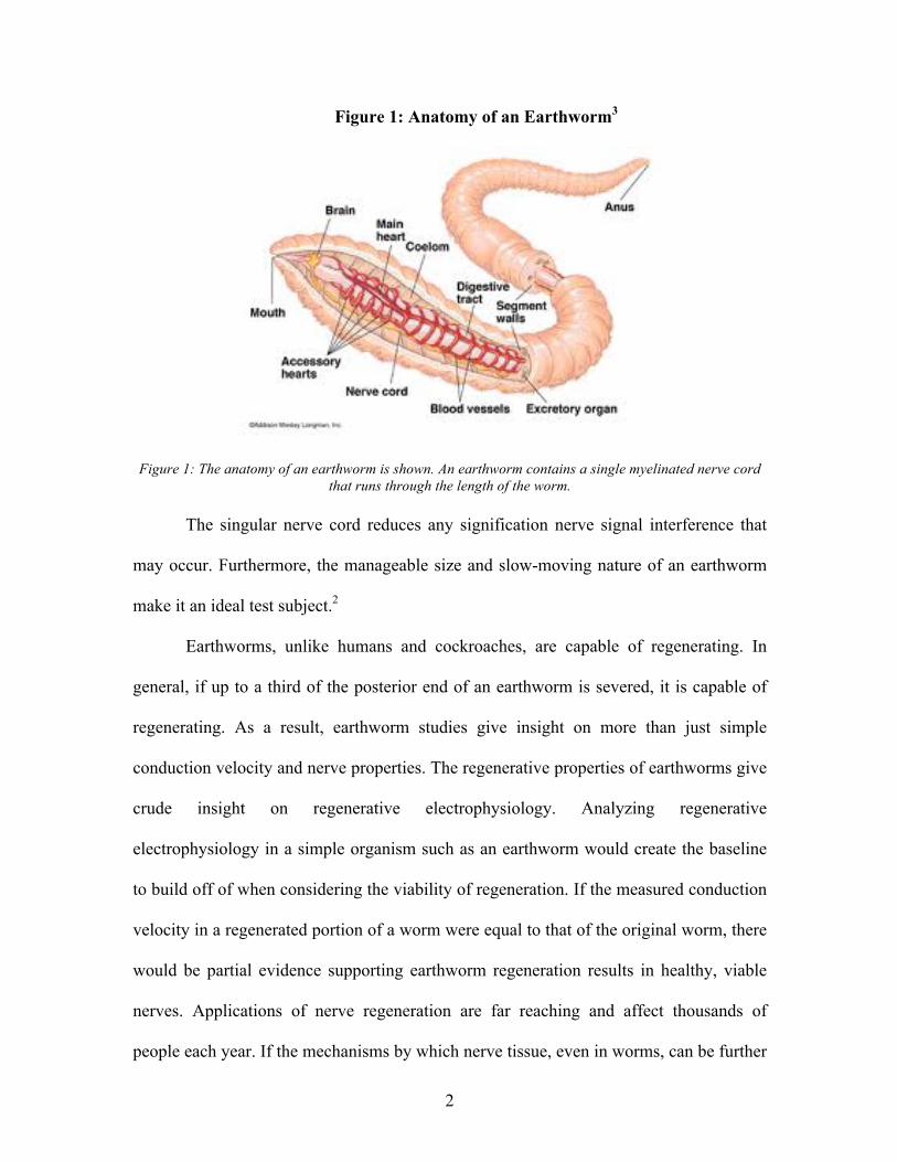
Figure 1: Anatomy of an Earthworm3

Figure 1: The anatomy of an earthworm is shown. An earthworm contains a single myelinated nerve cord that runs through the length of the worm.

The singular nerve cord reduces any signification nerve signal interference that

may occur. Furthermore, the manageable size and slow-moving nature of an earthworm

make it an ideal test subject.2

Earthworms, unlike humans and cockroaches, are capable of regenerating. In

general, if up to a third of the posterior end of an earthworm is severed, it is capable of

regenerating. As a result, earthworm studies give insight on more than just simple

conduction velocity and nerve properties. The regenerative properties of earthworms give

crude insight on regenerative electrophysiology. Analyzing regenerative

electrophysiology in a simple organism such as an earthworm would create the baseline

to build off of when considering the viability of regeneration. If the measured conduction

velocity in a regenerated portion of a worm were equal to that of the original worm, there

would be partial evidence supporting earthworm regeneration results in healthy, viable

nerves. Applications of nerve regeneration are far reaching and affect thousands of

people each year. If the mechanisms by which nerve tissue, even in worms, can be further

3

understood, the procedures through which neuroregeneration is initiated can be improved

and translated to more complex organisms.

4

Procedure:

Preparation for PicoScope and PicoLog Analysis

To measure the conduction velocity of intact and regenerated earthworms, the

programs PicoScope and PicoLog were used. A sample of worms were collected and kept

alive in a large bin of soil. A single worm was taken out at a time and anesthetized in a

prepared 10% ethanol solution for seven minutes. The anesthetized earthworm was

pinned dorsal side up, and the leads were attached to the worm in the following manner

(Figure 2).

Figure 2: Signal Capturing Schematic4

Figure 2: Two leads (R2 and R1) were placed two centimeters away from each other. A ground was placed anterior to R1.

The two leads, labeled as R2 and R1 in Figure 2, were placed approximately two

centimeters away from each other. For individual signal measurements plotted on the

same axis, each lead was attached to two different signal amplifiers. Both amplifiers were

configured as follows (Table 1):

Table 1: Amplifier Settings

Input Select Low Filter High Filter Mode Gain A 300 Hz 1 kHz AC 100

5

The amplifier corresponding to R1 was connected to the “Channel A” input of

PicoScope, while the amplifier corresponding to R2 was connected to the “Channel B”

input. The ground was connected to the Faraday cage that the earthworm was placed in.

Spontaneous Measurements of Earthworms

Baseline recordings were taken for 2-second intervals with 200 milliseconds per

division. These baseline recordings were made to distinguish between spontaneous and

evoked measurements.

Evoked Measurements of Earthworms

Upon taking these baselines, the posterior end of the worm was mechanically

stimulating with the end of a pen. Because two leads were plotted on the same axes, there

was a slight offset in time between the peaks measured by the more posterior lead and the

anterior lead. The data was analyzed in MATLAB to find the peaks that resulted from

mechanical stimulation (see Appendix I for sample code). The time offset in peak

location between leads A and B was measured and used to calculate the conduction

velocity by:

𝐶𝑜𝑛𝑑𝑢𝑐𝑡𝑖𝑜𝑛  𝑉𝑒𝑙𝑜𝑐𝑖𝑡𝑦 = !"#$%&'(  !"#$""%  !"#$%!"#$

[1]

where the distance between the leads was set as 2 centimeters.

Regenerated Earthworms

Once these recordings were performed, the posterior third of the same worms

were severed, and the worms were left to regenerate. The same worms were revisited

three days later; unfortunately, only one of the two worms was fully regenerated. The

same experimental procedure was followed to see if there was any significant difference

in conduction velocity between the intact and regenerated nerve. The conduction

6

velocities were compared, even though no statistical test could result in a strong

conclusion because of a small sample size.

7

Results and Discussion:

Spontaneous Measurements of Intact Earthworm

The intact earthworms naturally generated action potentials, making it necessary

to distinguish between spontaneous and evoked measurements. Therefore, baseline

recordings were taken for 2-second intervals with 200 milliseconds per division without

any mechanical stimulation. These evoked measurements were produced only at the R2

lead. The spontaneous recording is shown below (Figure 3).

Figure 3: Spontaneous Recordings of Normal Earthworm

Figure 3: The baseline recordings were taken to distinguish between spontaneous and evoked measurements.

As expected, the spontaneous recordings of the intact earthworm had action

potentials. None of these action potentials had a voltage of magnitude greater than 100

mV. Therefore, the threshold for a mechanically stimulated action potential was set to

100 mV.

8

Mechanical Stimulation of Intact Earthworm

After finding the threshold for mechanically stimulated action potentials, the trial

was repeated where both leads were considered. The earthworm was poked numerous

times with a pen, and the mechanically stimulated action potentials were recorded (Figure

4).

Figure 4: Mechanically Stimulated Action Potentials

Figure 4: The recording of mechanically stimulated action potentials, where lead R2 is in blue, and lead R1 is in green. When the stimulation was applied, an action potential greater than 200 mV was apparent.

As previously indicated, the mechanically stimulated action potentials would have

a magnitude greater than 100 mV. Specifically, they ranged from approximately 200 mV

to 400 mV. These mechanically stimulated action potentials resulted almost

instantaneously after poking the earthworm with the pen. From these action potentials,

data analysis techniques were applied to zoom in on the mechanically stimulated action

9

potentials for each lead, as shown below (Figure 5). This was necessary to determine the

conduction velocity, as the action potentials occurred so close to each other.

Figure 5: Identifying the Mechanically Stimulated Action Potentials

Figure 5: The mechanically stimulated action potential from Figure 4 was zoomed in on. The peaks of the action potentials for both leads were circled, as shown in the figure above. This allows for the conduction

velocity to be calculated.

The circles in red and black from Figure 5 indicate the position of where the

action potential peak was for leads R2 and R1, respectively. As expected, the action

potential for lead R2 occurred before the action potential for lead R1 because lead R2

was in the more posterior position. From these circles, the time at which these action

potentials were generated for each lead was determined. This process was repeated six

times, as shown in Table 2.

10

Table 2: Time of Action Potential for Each Lead

Trial R2 Peak Time (seconds) R1 Peak Time (seconds) 1 0.3314 0.3324 2 0.9992 1.0008 3 2.2826 2.2832 4 2.8223 2.8231 5 4.7801 4.7816 6 6.6399 6.6420

As a result, the conduction velocity from each trial was determined by recalling

that the leads were 2 centimeters apart (Table 3).

Table 3: Conduction Velocity for Each Trial

Trial Conduction Velocity (m/s) 1 19.8 2 12.4 3 33.4 4 24.4 5 13.3 6 9.5

From Table 3, the conduction velocity of the intact earthworm was calculated as

18.9 m/s ± 9.0 m/s. In order to have an unbiased control group, the data was only

generated for the single earthworm that regenerated after three days. Both earthworms

were severed in the posterior third, in hopes to have more samples. However, as indicated

previously, only one of the two earthworms regenerated after three days. This conduction

velocity was compared to the conduction velocity of the regenerated earthworm for

insight on electrophysiological differences between intact and regenerated earthworms. If

more time were available, more earthworms would have been studied for greater

statistical significance.

11

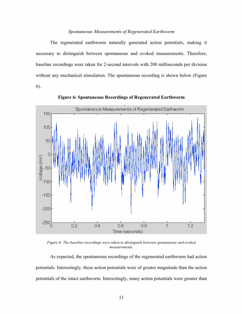
Spontaneous Measurements of Regenerated Earthworm

The regenerated earthworm naturally generated action potentials, making it

necessary to distinguish between spontaneous and evoked measurements. Therefore,

baseline recordings were taken for 2-second intervals with 200 milliseconds per division

without any mechanical stimulation. The spontaneous recording is shown below (Figure

6).

Figure 6: Spontaneous Recordings of Regenerated Earthworm

Figure 6: The baseline recordings were taken to distinguish between spontaneous and evoked measurements.

As expected, the spontaneous recordings of the regenerated earthworm had action

potentials. Interestingly, these action potentials were of greater magnitude than the action

potentials of the intact earthworm. Interestingly, many action potentials were greater than

12

100 mV for the regenerated earthworm, unlike the intact earthworm. This corresponded

with higher mechanically stimulated action potential magnitudes, as shown below.

Mechanical Stimulation of Regenerated Earthworm

After finding the threshold for mechanically stimulated action potentials, the trial

was repeated where both leads were considered. The earthworm was poked numerous

times with a pen, and the mechanically stimulated action potentials were recorded (Figure

7).

Figure 7: Mechanically Stimulated Action Potentials

Figure 7: The recording of mechanically stimulated action potentials, where lead R2 is in blue, and lead R1 is in green. When the stimulation was applied, an action potential greater than 200 mV was apparent.

As previously indicated, the mechanically stimulated action potentials had a

magnitude greater than 200 mV. Specifically, they ranged from approximately 300 mV to

500 mV, which was greater than the mechanically stimulated action potentials of the

intact earthworms. This was not expected, as it was initially postulated that regeneration

13

of tissue should result in greater internal resistance, and thus a lower magnitude

conduction velocity. This can be seen by examining the spatial decay length (𝜆) equation:

𝜆 = !!!!

[2]

As the internal resistance ri increases, the spatial decay length decreases, implying

the conduction velocity should decrease. Future work might include examining what

regenerative properties might result in a greater action potential magnitude following

mechanical stimulation.

These mechanically stimulated action potentials resulted almost immediately after

poking the earthworm with the pen. From these action potentials, data analysis techniques

were applied to zoom in on the mechanically stimulated action potentials for each lead, as

shown below (Figure 8). This was necessary to determine the conduction velocity, as the

action potentials occurred so close to each other.

Figure 8: Identifying the Mechanically Stimulated Action Potentials

Figure 8: The mechanically stimulated action potential from Figure 7 was zoomed in on. The peaks of the action potentials for both leads were circled, as shown in the figure above. This allows for the conduction

velocity to be calculated.

14

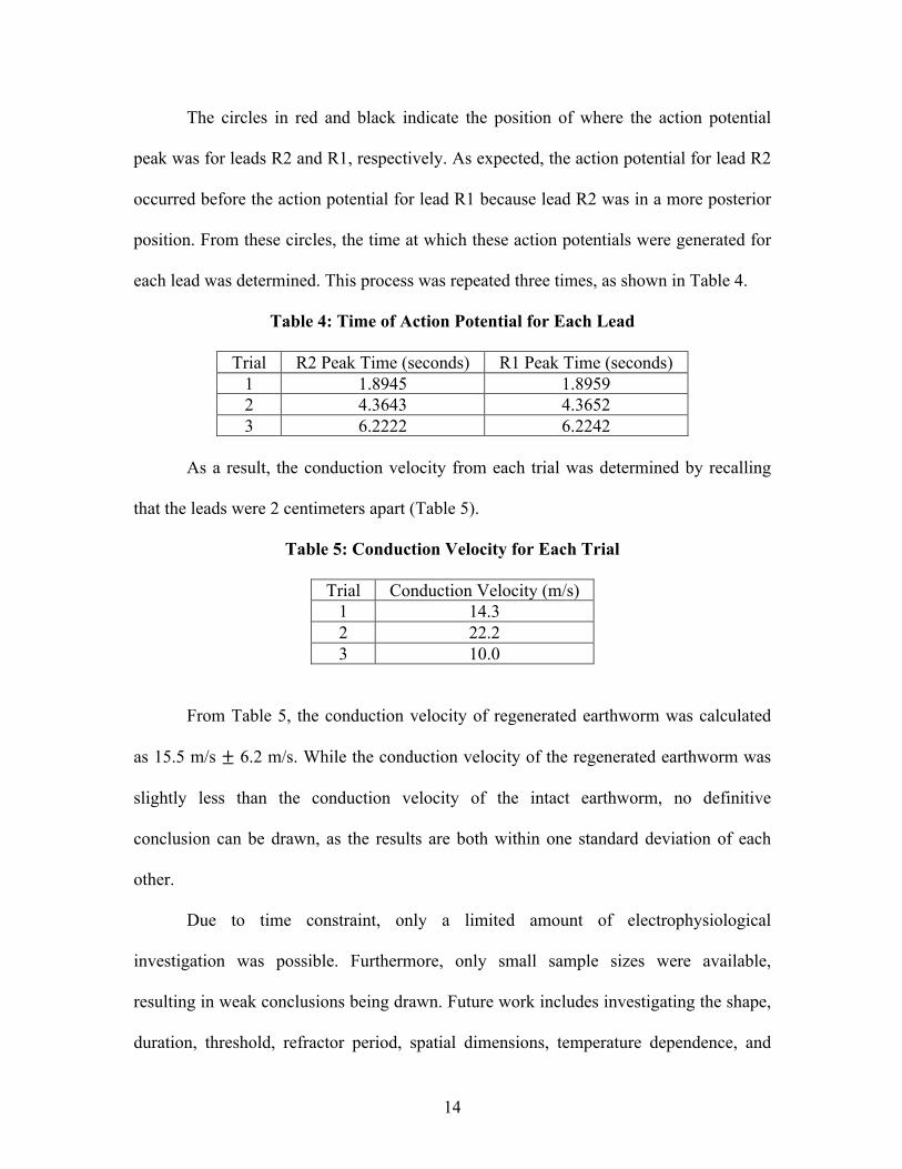
The circles in red and black indicate the position of where the action potential

peak was for leads R2 and R1, respectively. As expected, the action potential for lead R2

occurred before the action potential for lead R1 because lead R2 was in a more posterior

position. From these circles, the time at which these action potentials were generated for

each lead was determined. This process was repeated three times, as shown in Table 4.

Table 4: Time of Action Potential for Each Lead

Trial R2 Peak Time (seconds) R1 Peak Time (seconds) 1 1.8945 1.8959 2 4.3643 4.3652 3 6.2222 6.2242

As a result, the conduction velocity from each trial was determined by recalling

that the leads were 2 centimeters apart (Table 5).

Table 5: Conduction Velocity for Each Trial

Trial Conduction Velocity (m/s) 1 14.3 2 22.2 3 10.0

From Table 5, the conduction velocity of regenerated earthworm was calculated

as 15.5 m/s ± 6.2 m/s. While the conduction velocity of the regenerated earthworm was

slightly less than the conduction velocity of the intact earthworm, no definitive

conclusion can be drawn, as the results are both within one standard deviation of each

other.

Due to time constraint, only a limited amount of electrophysiological

investigation was possible. Furthermore, only small sample sizes were available,

resulting in weak conclusions being drawn. Future work includes investigating the shape,

duration, threshold, refractor period, spatial dimensions, temperature dependence, and

15

propagation of a larger sample size of normal and regenerated earthworm ventral nerve

cord.

16

Conclusion:

To improve regenerative therapeutics, it is necessary to better understand the

mechanisms and physiological effects of natural blastema regeneration. Therefore, the

conduction velocity of earthworm animal models was studied to crudely understand the

physiological effects of natural blastema regeneration. The conduction velocity of intact

and regenerated earthworms was calculated as 18.9 m/s ± 9.0 m/s and 15.5 m/s ± 6.2

m/s, respectively. These results indicate no significant difference can be drawn on intact

and regenerated earthworm conduction velocities. However, it was noted that the

magnitude of action potentials increased following regeneration, which was not expected.

Therefore, the mechanism resulting in a greater action potential magnitude will be

examined in the future. Future work also includes investigating the shape, duration,

threshold, refractor period, spatial dimensions, temperature dependence, and propagation

of a larger sample size of normal and regenerated earthworm ventral nerve cord.

17

References:

1 Kandel, Eric R., James H. Schwartz, and Thomas M. Jessell. Principles of Neural Science. New York: McGraw-Hill, Health Professions Division, 2000. Print. 2 Kladt, Nikolay, Ulrike Hanslik, Hans-Georg Heinzel. Teaching Basic Neurophysiology Using Intact Earthworms. The Journal of Undergraduate Neuroscience Education, 2010. 3 "Earthworms A Scientific Study | Complete Guide for Earthworms." HubPages. N.p., n.d. Web. 17 May 2013. <http://sukritha.hubpages.com/hub/EarthwormAfraidSalts>. 4 "Earthworm Action Potentials." ADInstruments. N.p., n.d. Web. 17 May 2013. <http://www.adinstruments.com/solutions/education/ltexp/earthworm-action-potentials>.

18

Appendix I:

Sample Code To Calculate Conduction Velocity

clear all; csvRange1 = [9800,0,(12053),0]; x = csvread('Mechanical Stimulation A-B_09.csv',9800,0,csvRange1); csvRange2 = [9800,1,(12053),1]; m = csvread('Mechanical Stimulation A-B_09.csv',9800,1,csvRange2); csvRange3 = [9800,2,(12053),2]; k = csvread('Mechanical Stimulation A-B_09.csv',9800,2,csvRange3); plot(x,m); hold all; plot(x,k); [pks,locs] = findpeaks(m,'MINPEAKHEIGHT',205); hold all; xxx = locs(13); plot(x(xxx),pks(13),'o'); [pks2,locs2] = findpeaks(k,'MINPEAKHEIGHT',200); hold all; xx = locs2(32); plot(x(xx),pks2(32),'o'); diff = abs(x(xx)-x(xxx)); vel=.02/diff;