The Conformal Monogenic Signal?

Lennart Wietzke and Gerald Sommer

Kiel University, Institute of Computer Science, Chair of Cognitive Systems,Christian-Albrechts-Platz 4, 24118 Kiel, Germany

lw,gs@ks.informatik.uni-kiel.de

Abstract. The conformal monogenic signal is a novel rotational invari-ant approach for analyzing i(ntrinsic)1D and i2D local features of two-dimensional signals (e.g. images) without the use of any heuristics. Itcontains the monogenic signal as a special case for i1D signals and com-bines scale-space, phase, orientation, energy and isophote curvature inone unified algebraic framework. The conformal monogenic signal willbe theoretically illustrated and motivated in detail by the relation ofthe Radon and the Riesz transform. One of the main ideas is to lift uptwo-dimensional signals to a higher dimensional conformal space wherethe signal can be analyzed with more degrees of freedom. The most in-teresting result is that isophote curvature can be calculated in a purelyalgebraic framework without the need of any derivatives.

1 Introduction

In this paper 2D signals (e.g. gray value images) f ∈ L2(Ω; R) with Ω ⊂ R2

will be locally analyzed. Features such as phase φ, orientation θ and curvatureκ will be determined at every test point (x, y) ∈ Ω of the original 2D signalf . For each test point a local coordinate system will be applied before analysis.One important local structural feature is the phase φ of a DC free 1D signalmodel g(x) := a(x) cos(φ(x)) which can be calculated by means of the Hilberttransform. Furthermore all signals will be analyzed in scale space (e.g. in Poissonscale space [1]) because the Hilbert transform can only be interpreted for narrowbanded signals. One possible generalization of the Hilbert transform to higherdimensions which will be used in this work is the Riesz transform. 2D signalsf are classified into local regions N ⊆ Ω of different intrinsic dimensions (alsoknown as codimension):

f ∈

i0DN , f(xi) = f(xj) ∀xi,xj ∈ Ni1DN , f(x, y) = g(x cos θ + y sin θ) ∀(x, y) ∈ N, f /∈ i0DN

i2DN , else. (1)

? We acknowledge funding by the German Research Foundation (DFG) under theproject SO 320/4-2

2

2 The Monogenic Signal

Phase and amplitude of 1D signals can be analyzed by the analytic signal. Thegeneralization of the analytic signal to multidimensional signal domains has beendone by the monogenic signal [2]. In case of 2D signals the monogenic signal de-livers local phase, orientation and energy information. The monogenic signal canbe interpreted for the application to i1D signals. This work presents the gener-alization of the monogenic signal for 2D signals to analyze both i1D and i2Dsignals in one single framework. The conformal monogenic signal delivers localphase, orientation, energy and curvature for i1D and i2D signals with the mono-genic signal as a special case. To illustrate the motivation and the interpretationof this work, first of all the monogenic signal will be recalled in detail.

2.1 Riesz Transform

The monogenic signal replaces the Hilbert transform of the analytic signal bythe Riesz transform which is known from Clifford analysis [3]. The Riesz trans-form R· extends the signal f to a monogenic (holomorphic) function. It isone possible, but not the only generalization of the Hilbert transform to multi-dimensional signal domains. In spatial domain the Riesz transform is given bythe following convolution [4]:

Rf(0) :=Γ (m+1

2 )

πm+1

2

∫x∈Rm

f(x)‖x‖m+1

x dx . (2)

In this work the Cauchy principal value (P.v.) of all integrals will be omitted. Toenable interpretation of the Riesz transform, its relation to the Radon transformwill be shown in detail. This relation can be proved by means of the Fourier slicetheorem [5].

2.2 Relation of the Riesz and Radon Transform

The Riesz transform can be expressed using the Radon and the Hilbert trans-form. Note that the relation to the Radon transform is required solely for inter-pretation and theoretical results. Neither the Radon transform nor its inverseare ever applied to the signal in practice. Instead the Riesz transformed signalwill be determined by convolution in spatial domain. The 2D Radon transform[6] is defined as:

r(t, θ) := Rf(t, θ) :=∫

(x,y)∈R2

f(x, y)δ0(x cos θ + y sin θ − t)d(x, y) (3)

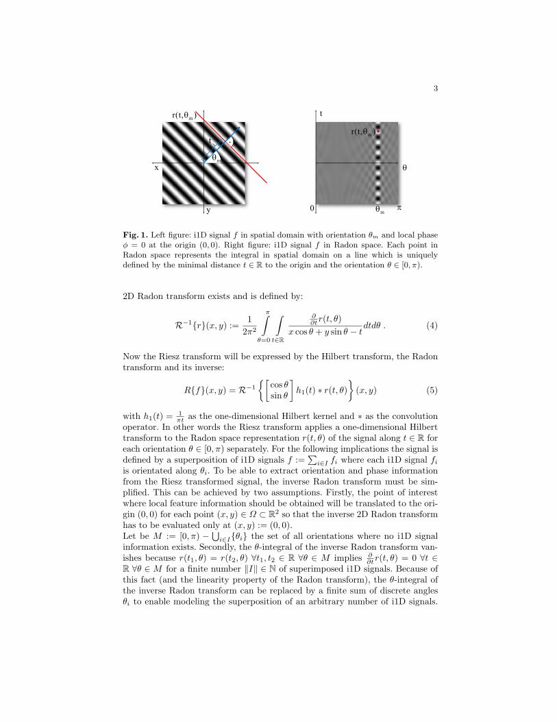
with θ ∈ [0, π) as the orientation, t ∈ R as the minimal distance of the line tothe origin (0, 0) and δ0 as the Dirac delta distribution (see figure 1). The inverse

3

x

y

t

mr(t, )θ

mθ

i

θ

t

mθ0 π

mr(t, )θ

Fig. 1. Left figure: i1D signal f in spatial domain with orientation θm and local phaseφ = 0 at the origin (0, 0). Right figure: i1D signal f in Radon space. Each point inRadon space represents the integral in spatial domain on a line which is uniquelydefined by the minimal distance t ∈ R to the origin and the orientation θ ∈ [0, π).

2D Radon transform exists and is defined by:

R−1r(x, y) :=1

2π2

π∫θ=0

∫t∈R

∂∂tr(t, θ)

x cos θ + y sin θ − tdtdθ . (4)

Now the Riesz transform will be expressed by the Hilbert transform, the Radontransform and its inverse:

Rf(x, y) = R−1

[cos θsin θ

]h1(t) ∗ r(t, θ)

(x, y) (5)

with h1(t) = 1πt as the one-dimensional Hilbert kernel and ∗ as the convolution

operator. In other words the Riesz transform applies a one-dimensional Hilberttransform to the Radon space representation r(t, θ) of the signal along t ∈ R foreach orientation θ ∈ [0, π) separately. For the following implications the signal isdefined by a superposition of i1D signals f :=

∑i∈I fi where each i1D signal fi

is orientated along θi. To be able to extract orientation and phase informationfrom the Riesz transformed signal, the inverse Radon transform must be sim-plified. This can be achieved by two assumptions. Firstly, the point of interestwhere local feature information should be obtained will be translated to the ori-gin (0, 0) for each point (x, y) ∈ Ω ⊂ R2 so that the inverse 2D Radon transformhas to be evaluated only at (x, y) := (0, 0).Let be M := [0, π) −

⋃i∈Iθi the set of all orientations where no i1D signal

information exists. Secondly, the θ-integral of the inverse Radon transform van-ishes because r(t1, θ) = r(t2, θ) ∀t1, t2 ∈ R ∀θ ∈ M implies ∂

∂tr(t, θ) = 0 ∀t ∈R ∀θ ∈ M for a finite number ‖I‖ ∈ N of superimposed i1D signals. Because ofthis fact (and the linearity property of the Radon transform), the θ-integral ofthe inverse Radon transform can be replaced by a finite sum of discrete anglesθi to enable modeling the superposition of an arbitrary number of i1D signals.

4

Therefore the inverse Radon transform can be written as:

R−1r(0, 0) = − 12π2

∑i∈I

∫t∈R

∂∂tr(t, θi)

tdt . (6)

Now the 2D Riesz transform and therefore the monogenic signal can be inter-preted in an explicit way.

2.3 Interpretation of the 2D Riesz Transform

Because of the property ∂∂t (h1(t) ∗ r(t, θ)) = h1(t)∗ ∂

∂tr(t, θ) the 2D Riesz trans-form of any i1D signal with orientation θm results in:[

Rxf(0, 0)Ryf(0, 0)

]= − 1

2π2

∫t∈R

1th1(t) ∗

∂

∂tr(t, θm)dt

︸ ︷︷ ︸=:s(θm)

[cos θm

sin θm

]. (7)

The orientation of the signal can therefore be derived by:

θm = arctans(θm) sin θm

s(θm) cos θm= arctan

Ryf(0, 0)Rxf(0, 0)

. (8)

The partial Hilbert transform [7] of fθm(τ) := f(τ cos θm, τ sin θm) and therefore

also its phase can be calculated by:

φ = atan2 ((h1 ∗ fθm)(0), f(0, 0)) (9)

= atan2(√

R2xf(0, 0) + R2

yf(0, 0), f(0, 0))

. (10)

This reveals that - although the Riesz transform is a generalization of the Hilberttransform to multi-dimensional signal domains - it still applies a one-dimensionalHilbert transform along the main orientation θm to the signal. In short, themonogenic signal enables interpretation of i1D signals and the mean value oftheir superposition [8].

3 The Conformal Monogenic Signal

The feature space of the 2D monogenic signal is spanned by phase, orientationand energy information. This restriction correlates to the dimension of the as-sociated Radon space. Therefore, the feature space of the 2D signal can onlybe extended by lifting up the original signal to higher dimensions. This is oneof the main ideas of the conformal monogenic signal. In the following the 2Dmonogenic signal will be generalized to analyze also i2D signals by embeddingthe 2D signal into the conformal space. The previous section shows that the 2DRiesz transform can be expressed by the 2D Radon transform which integratesall function values on lines. This restriction to lines is one of the reasons why

5

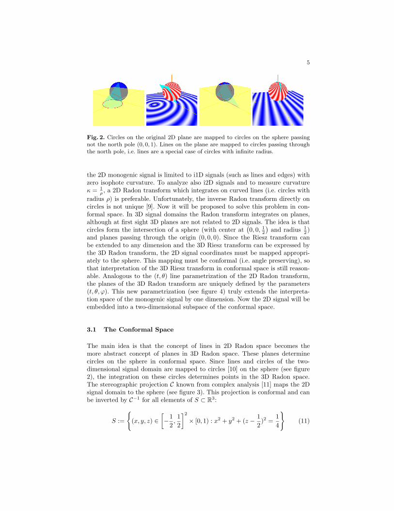
Fig. 2. Circles on the original 2D plane are mapped to circles on the sphere passingnot the north pole (0, 0, 1). Lines on the plane are mapped to circles passing throughthe north pole, i.e. lines are a special case of circles with infinite radius.

the 2D monogenic signal is limited to i1D signals (such as lines and edges) withzero isophote curvature. To analyze also i2D signals and to measure curvatureκ = 1

ρ , a 2D Radon transform which integrates on curved lines (i.e. circles withradius ρ) is preferable. Unfortunately, the inverse Radon transform directly oncircles is not unique [9]. Now it will be proposed to solve this problem in con-formal space. In 3D signal domains the Radon transform integrates on planes,although at first sight 3D planes are not related to 2D signals. The idea is thatcircles form the intersection of a sphere (with center at

(0, 0, 1

2

)and radius 1

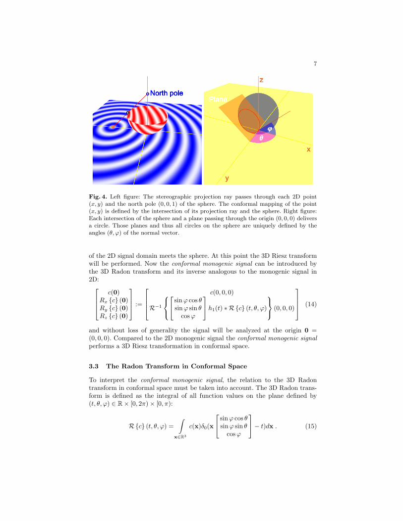
2 )and planes passing through the origin (0, 0, 0). Since the Riesz transform canbe extended to any dimension and the 3D Riesz transform can be expressed bythe 3D Radon transform, the 2D signal coordinates must be mapped appropri-ately to the sphere. This mapping must be conformal (i.e. angle preserving), sothat interpretation of the 3D Riesz transform in conformal space is still reason-able. Analogous to the (t, θ) line parametrization of the 2D Radon transform,the planes of the 3D Radon transform are uniquely defined by the parameters(t, θ, ϕ). This new parametrization (see figure 4) truly extends the interpreta-tion space of the monogenic signal by one dimension. Now the 2D signal will beembedded into a two-dimensional subspace of the conformal space.

3.1 The Conformal Space

The main idea is that the concept of lines in 2D Radon space becomes themore abstract concept of planes in 3D Radon space. These planes determinecircles on the sphere in conformal space. Since lines and circles of the two-dimensional signal domain are mapped to circles [10] on the sphere (see figure2), the integration on these circles determines points in the 3D Radon space.The stereographic projection C known from complex analysis [11] maps the 2Dsignal domain to the sphere (see figure 3). This projection is conformal and canbe inverted by C−1 for all elements of S ⊂ R3:

S :=

(x, y, z) ∈

[−1

2,12

]2

× [0, 1) : x2 + y2 + (z − 12)2 =

14

(11)

6

SR23 C(x, y) :=

1x2 + y2 + 1

xy

x2 + y2

, C−1(x, y, z) :=1

1− z

[xy

]. (12)

This mapping has the property that the origin (0, 0) of the 2D signal domain willbe mapped to the south pole 0 := (0, 0, 0) of the sphere and both−∞,+∞ will bemapped to the north pole (0, 0, 1) of the sphere. Lines and circles of the 2D signaldomain will be mapped to circles on the sphere and can be determined uniquelyby planes in 3D Radon space. The integration on these planes corresponds topoints (t, θ, ϕ) in the 3D Radon space.

Fig. 3. Left and right figure show the conformal space from two different point of views.The 2D signal f will be mapped by the stereographic projection on the sphere.

3.2 The Riesz Transform in Conformal Space

Since the signal domain Ω ⊂ R2 is bounded, not the whole sphere is covered bythe original signal (see left part of figure 4). Anyway, all planes correspondingto circles remain unchanged. That is the reason why the conformal monogenicsignal models i1D lines and all kinds of curved i2D signals which can be locallyapproximated by circles. To give the Riesz transform more degrees of freedom,the original two-dimensional signal will be embedded in a applicable subspaceof the conformal space by:

RR33 c(x, y, z) :=

f(C−1(x, y, z)T ) , x2 + y2 +

(z − 1

2

)2 = 14

0 , else. (13)

Thus, the 3D Riesz transform can be applied to all points on the sphere. Thecenter of convolution in spatial domain is the south pole (0, 0, 0) where the origin

7

North pole o

o

o

4

q

Plane

z

x

y

Fig. 4. Left figure: The stereographic projection ray passes through each 2D point(x, y) and the north pole (0, 0, 1) of the sphere. The conformal mapping of the point(x, y) is defined by the intersection of its projection ray and the sphere. Right figure:Each intersection of the sphere and a plane passing through the origin (0, 0, 0) deliversa circle. Those planes and thus all circles on the sphere are uniquely defined by theangles (θ, ϕ) of the normal vector.

of the 2D signal domain meets the sphere. At this point the 3D Riesz transformwill be performed. Now the conformal monogenic signal can be introduced bythe 3D Radon transform and its inverse analogous to the monogenic signal in2D:

c(0)Rx c (0)Ry c (0)Rz c (0)

:=

c(0, 0, 0)

R−1

sinϕ cos θ

sinϕ sin θcos ϕ

h1(t) ∗ Rc (t, θ, ϕ)

(0, 0, 0)

(14)

and without loss of generality the signal will be analyzed at the origin 0 =(0, 0, 0). Compared to the 2D monogenic signal the conformal monogenic signalperforms a 3D Riesz transformation in conformal space.

3.3 The Radon Transform in Conformal Space

To interpret the conformal monogenic signal, the relation to the 3D Radontransform in conformal space must be taken into account. The 3D Radon trans-form is defined as the integral of all function values on the plane defined by(t, θ, ϕ) ∈ R× [0, 2π)× [0, π):

Rc (t, θ, ϕ) =∫

x∈R3

c(x)δ0(x

sinϕ cos θsinϕ sin θ

cos ϕ

− t)dx . (15)

8

Since the signal is mapped on the sphere and all other points of the conformalspace are set to zero, the 3D Radon transform actually sums up all points lyingon the intersection of the plane and the sphere. For all planes this intersectioncan be either empty or a circle. The concept of circles in the conformal 3DRadon transform can be compared with the concept of lines known from the2D Radon transform. Since lines in the 2D domain are also mapped to circles,the conformal monogenic signal can analyze i1D as well as curved i2D signals inone single framework. The inverse 3D Radon transform exists and differs fromthe 2D case such that it is a local transformation [12]. That means the Riesztransform at (0, 0, 0) is completely determined by all planes passing the origin(i.e. t = 0). In contrast, the 2D monogenic signal requires all integrals on alllines (t, θ) to reconstruct the original signal at a certain point and is thereforecalled a global transform. This interesting fact turns out from the following 3Dinverse Radon transform:

R−1r(0) := − 18π2

2π∫θ=0

π∫ϕ=0

∂2

∂t2r(t, θ, ϕ)|t=0 dϕdθ . (16)

Therefore, the local features of i1D and i2D signals can be determined by theconformal monogenic signal at the origin of the 2D signal without knowledge ofthe whole Radon space. Hence, the relation of the Radon and the Riesz transformis essential to interpret the Riesz transform in conformal space.

3.4 Interpretation and Experimental Results

Analogous to the interpretation of the monogenic signal, the parameters of theplane within the 3D Radon space determine the local features of the curved i2Dsignal. The conformal monogenic signal can be called the generalized monogenicsignal for i1D and i2D signals, because lines and edges can be considered as circleswith zero curvature. These lines are mapped to circles passing through the northpole in conformal space. The curvature can be measured by the parameter ϕ ofthe 3D Radon space:

ϕ = arctanRz c (0)√

R2x c (0) + R2

y c (0). (17)

It can be shown that ϕ corresponds to the isophote curvature κ known fromdifferential geometry [13, 14]:

κ =−fxxf2

y + 2fxfyfxy − fyyf2x(

f2x + f2

y

) 32

. (18)

Besides, the curvature of the conformal monogenic signal naturally indicatesthe intrinsic dimension of the signal. The parameter θ will be interpreted as theorientation in i1D case and deploys to direction θ ∈ [0, 2π) for the i2D case:

θ = atan2 (Ry c (0), Rx c (0)) . (19)

9

The phase is defined by φ for all intrinsic dimensions by

φ = atan2(√

R2x c (0) + R2

y c (0) + R2z c (0), c(0)

). (20)

All proofs are analogous to those shown for the 2D monogenic signal. The con-formal monogenic signal can be efficiently implemented by convolution in spatialdomain without the need of any Fourier transform. Since the 3D convolution inconformal space can be simplified to a faster 2D convolution on the sphere, thetime complexity of the conformal monogenic signal computation is in O(n2) withn as the convolution mask size in one dimension. On synthetic signals the error ofthe feature extraction converges to zero with increasing refinement of the convo-lution mask. The advantages of the monogenic isophote curvature compared tothe curvature delivered by the classical differential geometry [15] approach canbe seen clearly in figure 5. Under the presence of noise the monogenic isophotecurvature performs in general more robust than the classical isophote curvature.Detailed application and performance behavior of the conformal monogenic sig-nal will be part of future work.

Fig. 5. Experimental results and comparison. Top row from left to right: Syntheticsignal, monogenic isophote curvature and classical isophote curvature determined byderivatives. Bottom row from left to right: Energy, phase and direction. Convolutionmask size: 5× 5 pixels.

10

4 Conclusion

In this paper a novel generalization of the monogenic signal for two-dimensionalsignals has been presented to analyze i(ntrinsic)1D and i2D signals in one unifiedalgebraic framework. The idea of the conformal monogenic signal is to lift uptwo-dimensional signals to an appropriate conformal space in which the signalcan be Riesz transformed with more degrees of freedom compared to the 2Dmonogenic signal. Without steering i1D and i2D local features such as phase,orientation/direction, energy and isophote curvature can be determined in spa-tial domain. The conformal monogenic signal can be computed efficiently withsame time complexity as the 2D monogenic signal. Furthermore, the exact localisophote curvature (which is of practical importance in low level image analysis)can be calculated without the need of derivatives. Hence, all problems of partialderivatives on discrete grids can be avoided by the application of the conformalmonogenic signal.

References

1. Felsberg, M., Sommer, G.: The monogenic scale-space: A unifying approach tophase-based image processing in scale-space. Journal of Mathematical Imagingand Vision (2003)

2. Felsberg, M., Sommer, G.: The monogenic signal. Technical report, Kiel University(2001)

3. Brackx, F., De Knock, B., De Schepper, H.: Generalized multidimensional hilberttransforms in clifford analysis. International Journal of Mathematics and Mathe-matical Sciences (2006)

4. Delanghe, R.: Clifford analysis: History and perspective. In: Computational Meth-ods and Function Theory. Volume 1. (2001) 107–153

5. Stein, E.M.: Singular Integrals and Differentiability Properties of Functions.Princeton University Press (1971)

6. Beyerer, J., Leon, F.P.: The radon transform in digital image processing. Automa-tisierungstechnik 50(10) (2002) 472–480

7. Hahn, S.L.: Hilbert Transforms in Signal Processing. Artech House (1996)8. Wietzke, L., Sommer, G., Schmaltz, C., Weickert, J.: Differential geometry of

monogenic signal representations. In: Robot Vision, Springer (2008) 454–4659. Ambartsoumian, G., Kuchment, P.: On the injectivity of the circular radon trans-

form. In: Inverse Problems. Volume 21., Inst. of Physics Publishing (2005) 47310. Needham, T.: Visual Complex Analysis. Oxford University Press (1997)11. Gurlebeck, K., Habetha, K., Sprossig, W.: Funktionentheorie in der Ebene und im

Raum (Grundstudium Mathematik). Birkhauser Basel (2006)12. Bernstein, S.: Inverse probleme. Technical report, TU Bergakdemie Freiberg (2007)13. do Carmo, M.P.: Differential Geometry of Curves and Surfaces. Prentice-Hall

(1976)14. Baer, C.: Elementare Differentialgeometrie. Volume 1. de Gruyter, Berlin, New

York (2001)15. Lichtenauer, J., Hendriks, E.A., Reinders, M.J.T.: Isophote properties as features

for object detection. In: CVPR (2), IEEE Computer Society (2005) 649–654