the core collapse supernova rate in the sdss-ii supernova
TRANSCRIPT
Wayne State University
Wayne State University Dissertations
1-1-2011
The core collapse supernova rate in the sdss-iisupernova surveyMatthew Frederick TaylorWayne State University,
Follow this and additional works at: http://digitalcommons.wayne.edu/oa_dissertations
Part of the Astrophysics and Astronomy Commons, and the Physics Commons
This Open Access Dissertation is brought to you for free and open access by DigitalCommons@WayneState. It has been accepted for inclusion inWayne State University Dissertations by an authorized administrator of DigitalCommons@WayneState.
Recommended CitationTaylor, Matthew Frederick, "The core collapse supernova rate in the sdss-ii supernova survey" (2011). Wayne State UniversityDissertations. Paper 335.
THE CORE COLLAPSE SUPERNOVA RATE IN THE SDSS-IISUPERNOVA SURVEY
by
MATTHEW F. TAYLOR
DISSERTATION
Submitted to the Graduate School
of Wayne State University,
Detroit, Michigan
in partial fulfillment of the requirements
for the degree of
DOCTOR OF PHILOSOPHY
2011
MAJOR: Physics
Approved by:
Advisor Date
ACKNOWLEDGEMENTS
In addition to thanking Prof. Cinabro for his steady guidance and near infinite patience,
my thanks go to Prof. Sean Gavin, Prof. Ratna Naik, and the WSU Dept. of Physics
and Astronomy as a whole for helping me develop as a student, researcher and teacher. I
also would like to thank Rick Kessler, Joshua Frieman, Ben Dilday, Masao Sako, and other
members of the SDSS-II SN Survey Collaboration for many fruitful discussions and assistance
with data analysis.
ii
TABLE OF CONTENTS
Acknowledgments . . . . . . . . . . . . . . . . . . . . . . . . . . . . . . . . . . . . ii
List of Figures . . . . . . . . . . . . . . . . . . . . . . . . . . . . . . . . . . . . . . v
List of Tables . . . . . . . . . . . . . . . . . . . . . . . . . . . . . . . . . . . . . . viii
1 Introduction 1
1.1 Overview . . . . . . . . . . . . . . . . . . . . . . . . . . . . . . . . . . . . . . 1
1.2 History of Supernova Observation . . . . . . . . . . . . . . . . . . . . . . . . 2
1.3 Observational Characteristics of Supernovae . . . . . . . . . . . . . . . . . . 4
1.4 Current Physical Theory of Supernovae . . . . . . . . . . . . . . . . . . . . . 8
1.5 Star Formation and Stellar Evolution . . . . . . . . . . . . . . . . . . . . . . 12
1.6 Motivation for Measuring Core Collapse Rates . . . . . . . . . . . . . . . . . 15
1.7 Previous Supernova Rate Measurements . . . . . . . . . . . . . . . . . . . . 16
2 The SDSS-II Supernova Survey 17
2.1 Astronomical Surveys . . . . . . . . . . . . . . . . . . . . . . . . . . . . . . . 17
2.2 A Brief History of SDSS . . . . . . . . . . . . . . . . . . . . . . . . . . . . . 18
2.3 The SDSS-II Supernova Search Program . . . . . . . . . . . . . . . . . . . . 20
2.4 SDSS-II Type Ia Supernova Rate Results . . . . . . . . . . . . . . . . . . . . 23
2.5 BOSS Object Identifications and Redshift Measurements . . . . . . . . . . . 25
3 Rate Measurement Technique 26
3.1 Candidate Selection . . . . . . . . . . . . . . . . . . . . . . . . . . . . . . . . 26
iii
3.2 Phenomenological Light Curve Fitting . . . . . . . . . . . . . . . . . . . . . 30
3.3 Removal of Core Collapse Impostors . . . . . . . . . . . . . . . . . . . . . . 36
3.4 Luminosity, Distance and Volume Measurement . . . . . . . . . . . . . . . . 44
3.5 Supernova Time and Luminosity . . . . . . . . . . . . . . . . . . . . . . . . . 47
3.6 Supernova Detection Efficiency Model . . . . . . . . . . . . . . . . . . . . . . 48
3.7 Host Galaxy Extinction Model . . . . . . . . . . . . . . . . . . . . . . . . . . 53
4 Results 55
4.1 Supernova Count . . . . . . . . . . . . . . . . . . . . . . . . . . . . . . . . . 55
4.2 Corrections . . . . . . . . . . . . . . . . . . . . . . . . . . . . . . . . . . . . 59
4.3 Sources of Error . . . . . . . . . . . . . . . . . . . . . . . . . . . . . . . . . . 61
4.4 Division by Survey Time and Volume . . . . . . . . . . . . . . . . . . . . . . 62
5 Conclusion 64
5.1 Comparison with Prior Measurements . . . . . . . . . . . . . . . . . . . . . . 64
5.2 Implications for Star Formation . . . . . . . . . . . . . . . . . . . . . . . . . 66
5.3 The CCSN Luminosity Function . . . . . . . . . . . . . . . . . . . . . . . . . 68
5.4 Potential for Future Measurements . . . . . . . . . . . . . . . . . . . . . . . 70
Appendix A: Rate Sample Light Curves 73
Appendix B: Rate Sample Candidates 85
Bibliography . . . . . . . . . . . . . . . . . . . . . . . . . . . . . . . . . . . . . . 89
Abstract . . . . . . . . . . . . . . . . . . . . . . . . . . . . . . . . . . . . . . . . . 92
Autobiographical Statement . . . . . . . . . . . . . . . . . . . . . . . . . . . . . . 93
iv
LIST OF FIGURES
1.1 Supernova light curves are shown for various supernova types [4] . . . . . . 5
1.2 Supernova spectra are shown for various supernova types [4] . . . . . . . . . 6
1.3 Supernova types are defined by absorption features in their spectra . . . . . 7
1.4 This mosaic image of the Crab Nebula was taken by HST [8] . . . . . . . . 9
2.1 The progression of historical astronomical surveys is shown, along with pro-
jections for one future survey, LSST. The y coordinate represents the spatial
volume over which each survey reliably detected stars or galaxies. . . . . . . 18
2.2 SDSS photometric filter transmission curves are compared to spectra of several
celestial objects by L. Girardi et al (2002). [19] . . . . . . . . . . . . . . . . 19
2.3 The Hubble Diagram is shown, including the first year of SDSS-II SN data [21]. 22
2.4 The SN Ia Rate from Dilday et al. [23] and previous work is shown. . . . . . 24
3.1 Stripe 82, the SDSS-II Supernova Survey region, is shaded in red . . . . . . 27
3.2 False color composites of images submitted to human visual scan, including
an accepted supernova and some rejected images, are displayed in the SDSS-II
scanning guide [28]. . . . . . . . . . . . . . . . . . . . . . . . . . . . . . . . 29
3.3 The SDSS-II Supernova Survey data analysis pipeline condenses raw telescope
data into supernova candidate light curves. . . . . . . . . . . . . . . . . . . 30
3.4 Model light curve functions are compared when varying a single parameter at
a time. . . . . . . . . . . . . . . . . . . . . . . . . . . . . . . . . . . . . . . 32
v
3.5 SDSS-II SN candidate light curves are shown for which the light curve model
did not converge to a best fit. . . . . . . . . . . . . . . . . . . . . . . . . . . 34
3.6 SDSS-II SN candidate light curves are shown for which the light curve model
did not converge to a best fit. . . . . . . . . . . . . . . . . . . . . . . . . . . 35
3.7 Flatness score distribution is shown for all candidates, for confirmed super-
novae, and for confirmed AGN. . . . . . . . . . . . . . . . . . . . . . . . . . 37
3.8 Above are examples of confirmed AGN light curves, with the best model fit
plotted in green and the trivial, constant flux fit in blue. All these candidates
were excluded by the flatness requirement. . . . . . . . . . . . . . . . . . . 39
3.9 Above are examples of confirmed AGN light curves. All were excluded by the
flatness requirement. . . . . . . . . . . . . . . . . . . . . . . . . . . . . . . . 40
3.10 Above are examples from the accepted core collapse supernova rate sample. 42
3.11 Above are examples from the accepted core collapse supernova rate sample . 43
3.12 The redshift distribution of the raw CCSN rate sample is shown. . . . . . . 45
3.13 The supernova count is plotted versus limiting apparent magnitude. . . . . 50
3.14 The model supernova detection efficiency is shown. . . . . . . . . . . . . . . 51
3.15 The redshift distribution of the CCSN rate sample is shown, subluminous
candidates excluded, before and after the efficiency correction. . . . . . . . 52
4.1 Peak time distribution is shown for all candidates within the time and angle
constraints discussed in the text. A peak magnitude requirement shows that
systematic time bias primarily affects very dim objects. . . . . . . . . . . . 57
4.2 The peak apparent magnitude distribution, in SDSS r band, is shown for SN
candidates excluded from the rate sample for lack of redshift information. . 58
vi
5.1 The CCSN rate measurement from this work is shown with previous CCSN
rate measurements in the literature, as given by Horiuchi et al. [40] The solid
line is the best fit to ρ = ρ0(1 + z)a, with dashed lines indicating uncertainty.
The blue shaded region and nearby points represent the star formation rate
estimated primarily from the UV galaxy luminosity data of Baldry et al. [41]. 67
5.2 Historical CCSN rate and star formation rate measurements, from Horiuchi
et al. [40], are updated with results from this work. . . . . . . . . . . . . . . 69
5.3 A CCSN luminosity function is derived for the rate sample in this work, plus
candidates excluded only because they were faint or too near Earth. . . . . 71
vii
LIST OF TABLES
4.1 SNIa Removed from CCSN Rate Sample, by Identification Method, as defined
by Sako et al. [31] . . . . . . . . . . . . . . . . . . . . . . . . . . . . . . . . 59
4.2 Candidates Removed from CCSN Rate Sample, by Status and Redshift . . . 60
4.3 Corrections to the CCSN Rate Sample Size, by Reason . . . . . . . . . . . . 60
4.4 Sources of Error in the CCSN Rate . . . . . . . . . . . . . . . . . . . . . . . 62
4.5 Survey Time Ranges Included in CCSN Rate Measurement . . . . . . . . . 63
5.1 Polynomial Expansion of CCSN Rate vs. Redshift . . . . . . . . . . . . . . 66
viii
1
Chapter 1
Introduction
1.1 Overview
I begin this thesis with a brief history of supernova observation, and the gradual ac-
cumulation of scientific understanding up to the contemporary state of supernova science.
I describe the two major observational classes of supernovae, core collapse and thermonu-
clear, along with the current physical model for each as a consequence of stellar evolution.
From this, I relate the observed rate of core collapse supernova events to star formation,
and to other astrophysical phenomena of interest to science. I finish this first section with a
summary of core collapse supernova surveys from the literature, highlighting the additional
contribution from the present work.
Next, I present an overview of the Sloan Digital Sky Survey, focusing on the second
generation of the Sloan survey (SDSS-II) and on the SDSS-II Supernova Survey (SDSS-II
SN) collaboration within the overall project. I review major results of SDSS-II SN, including
cosmology measurements and thermonuclear (type Ia) supernova rate measurements.
In the third chapter, I describe how core collapse supernova (CCSN) candidates were
extracted from the full SDSS-II SN sample. I fit a phenomenological supernova light curve
model to the data, per the method developed by the SNLS collaboration [1]. I apply cuts to
2
remove objects deemed unlikely to be supernovae, and develop an efficiency model to correct
for supernovae undetected due to systematic observational constraints.
In the fourth section, I limit the supernova sample to a single volume-limited bin, from
redshift 0.03 to 0.09. In this redshift range, I can reliably identify core collapse events by
the lack of good fit to type Ia supernova light curve models.
I compare the present results with previous CCSN rate measurements, confirming the
trend predicted by the most recent of those studies. I explore conclusions from the com-
bined present and previous work, including cosmic star formation history and the supernova
luminosity distribution. Finally, I offer opportunities for future research building on this
work.
1.2 History of Supernova Observation
Since ancient times, observers of the heavens have known that most stars are unchanging
in brightness and relative position, at least on human time scales. However, there are notable
exceptions. Five “wandering stars” visible with the naked eye were named planets, a word
derived from the Greek “planes” (to wander), since they appear to wander among the other,
fixed stars in cyclic patterns on the sky. Today we know these to be the five nearest planets
in our own solar system.
Another exception to the fixed, unchanging nature of the heavens are occasional “guest
stars”, stars fixed in position relative to the other stars, but appearing where no star was
previously observed, then diminishing with time. The earliest recorded guest star is described
on Chinese bone engravings dated to 1300 BC, describing a bright new star appearing near
Antares [2].
An even brighter new star was observed in 1006 AD, in the southern constellation of
Lupus. The Egyptian astronomer Ali b. Ridwan wrote that the object was visibly round
in shape and size, appearing more than twice as large as Venus, bright enough to light
3
the horizon and shine more than a quarter as bright as the moon. References to the 1006
event are also found in other Arab writings of the period, along with Chinese, Japanese and
European records. Additional guest stars were recorded in 1054 AD near the constellation
of Taurus, and in 1181 AD near the constellation of Cassiopeia.
The first guest star for which we have a reliable, quantitative record occurred in 1572 AD
in the constellation of Cassiopeia. This object was made famous by Tycho Brahe in his work
“De Stella Nova” (Latin for “On the New Star”); this work popularized the term “stella
nova”, later shortened to “nova”, when referring to new stars. Brahe’s precise measurements
showed that the nova had no detectable parallax and no proper motion relative to other
stars, thus it must lie at a much greater distance than the planets. Brahe’s student, Johannes
Kepler, reached the same conclusion measuring a second nova in 1604 AD.
Another half-dozen or so novae were recorded by European astronomers in the 17th and
18th century, aided by the invention of the telescope. In the 19th century, the rate of nova
discovery greatly increased; more than 30 novae were found between 1840 and 1901 [3]. One
such event, Nova Persei 1901, occurred in a nebula of gas and dust, such that the nova’s
“light echo” could be seen propagating through the nebula. By measuring the echo’s angular
rate of change as seen from Earth, astronomers deduced that the nova occurred about 500
light years away.
This posed a challenge for the emerging theory of “spiral nebulae” as galaxies beyond
the Milky Way. An earlier nova, S Andromedae, was observed in the year 1885, and it was
apparently located inside the M31 spiral nebula. If this spiral nebula were a distant galaxy,
it would imply that S Andromedae had more than 10,000 times the intrinsic luminosity of
other novae like Nova Persei 1901. Of course, later evidence from many sources confirmed
that indeed the spiral nebulae are distant galaxies, implying that S Andromedae was an
exceptionally bright event, in a separate class from ordinary novae. In 1931, Fritz Zwicky
coined the term “super-novae” to refer to these stellar explosions, and by 1938 the hyphen
had been dropped. Astronomers have referred to this class of exceptionally bright new stars
4
as “supernovae” ever since.
1.3 Observational Characteristics of Supernovae
Supernovae are defined by their intense luminosity, which distinguishes them from ordi-
nary novae. Even the brightest novae are more than 600 times less luminous than a typical
supernova. A supernova’s brightness is usually quantified by its peak magnitude, a loga-
rithmic scale for the energy flux observed from the supernovae at the moment of maximum
luminosity. Magnitude is formally defined as:
m = −2.5log10(F
F0
) (1.1)
where F is the object’s observed flux in Janskys (1Jy = 10−26W/(m2Hz)), F0 is the flux
of a reference star (usually Vega) in the same units, and m is the resulting magnitude. Note
that brighter objects have lower magnitude, somewhat contrary to intuition.
Supernovae are also rather infrequent, occurring in a galaxy about once per 100 years,
on average. In our own Milky Way galaxy, it is believed that the bright “guest stars” of
1300 BC, 1066 AD, 1054 AD and 1181 AD were all supernovae, along with the “stella nova”
studied by Brahe and Kepler. Unfortunately for modern astronomers, no supernova has been
observed in our galaxy since the 17th century, though some may have occurred in regions of
our galaxy obscured from Earth by interstellar dust.
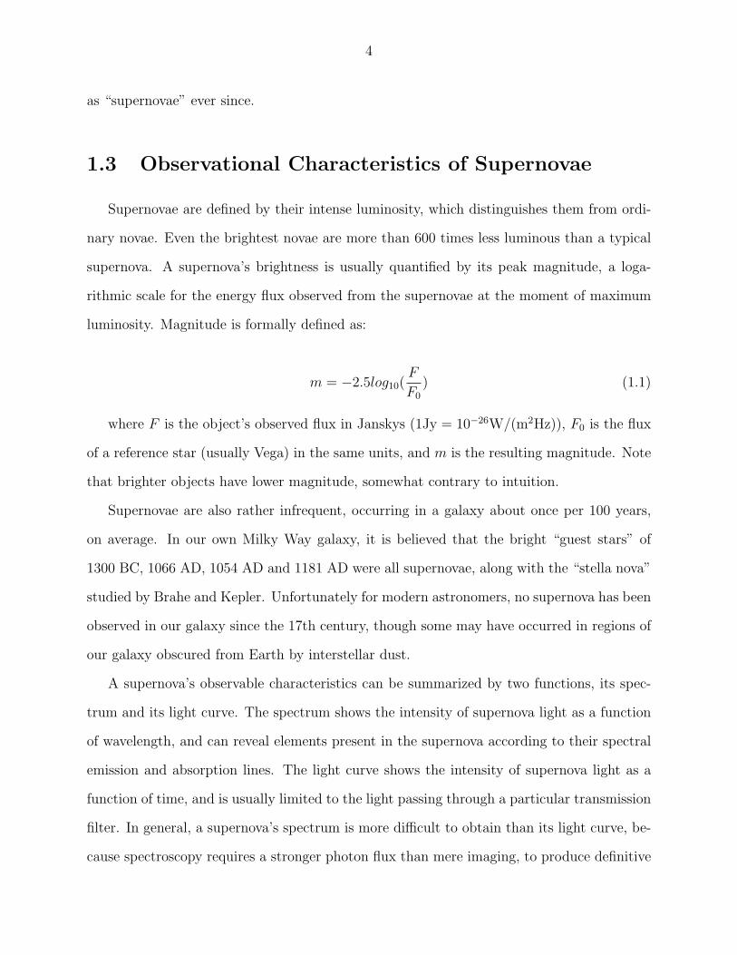
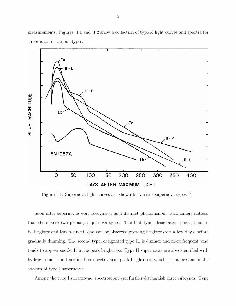
A supernova’s observable characteristics can be summarized by two functions, its spec-
trum and its light curve. The spectrum shows the intensity of supernova light as a function
of wavelength, and can reveal elements present in the supernova according to their spectral
emission and absorption lines. The light curve shows the intensity of supernova light as a
function of time, and is usually limited to the light passing through a particular transmission
filter. In general, a supernova’s spectrum is more difficult to obtain than its light curve, be-
cause spectroscopy requires a stronger photon flux than mere imaging, to produce definitive
5
measurements. Figures 1.1 and 1.2 show a collection of typical light curves and spectra for
supernovae of various types.
Figure 1.1: Supernova light curves are shown for various supernova types [4]
Soon after supernovae were recognized as a distinct phenomenon, astronomers noticed
that there were two primary supernova types. The first type, designated type I, tend to
be brighter and less frequent, and can be observed growing brighter over a few days, before
gradually dimming. The second type, designated type II, is dimmer and more frequent, and
tends to appear suddenly at its peak brightness. Type II supernovae are also identified with
hydrogen emission lines in their spectra near peak brightness, which is not present in the
spectra of type I supernovae.
Among the type I supernovae, spectroscopy can further distinguish three subtypes. Type
6
Figure 1.2: Supernova spectra are shown for various supernova types [4]
7
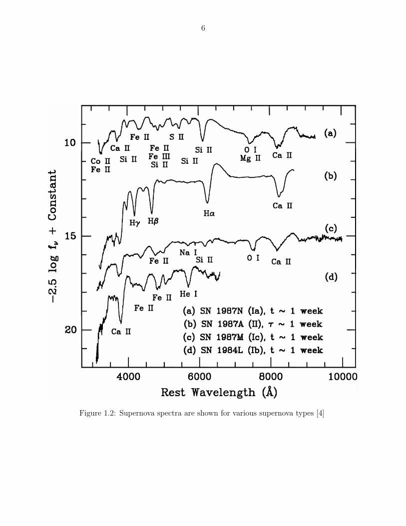
Ia supernovae show a strong absorption line at λ = 615.0nm near peak luminosity, corre-
sponding to singly ionized silicon (Si II). Type Ib show no silicon absorption, but do exhibit
a neutral helium absorption line at λ = 587.6nm. The remainder, showing neither silicon
nor helium absorption lines, are identified as type Ic.
Figure 1.3: Supernova types are defined by absorption features in their spectra
Type II supernovae have been further classified as well. The most common subtypes are
II-P, characterized by a plateau of roughly constant brightness in the light curve just after
peak, and II-L, which lacks a plateau and whose magnitude decays linearly with time. More
exotic subtypes include IIn, with exceptionally narrow absorption lines in their spectra, and
IIb, an apparent hybrid of type II and type Ib attributes. A number of unique type II
8
supernovae defy any of these classification schemes, and are simply called “type II peculiar”,
abbreviated “IIpec”.
A third class of supernovae has been proposed to include a handful of objects such as
SN2002bj that do not fit well into either type I or type II [5]. These dim supernovae, dubbed
“type .Ia”, have spectra similar to type IIn but evolve much more quickly than either type
I or type II supernovae. Since these events are relatively rare, more observation will be
required to better understand them.
1.4 Current Physical Theory of Supernovae
The current consensus is that the observational supernova classes derive from two distinct
physical events. Type Ia corresponds to thermonuclear supernovae, thought to occur when a
white dwarf star acquires sufficient mass from a companion star to exceed the Chandrasekhar
mass. The other supernova types (II, Ib and Ic) are core collapse supernovae, when the core
of a massive star makes a sudden transition to neutron star density, causing an explosive
rebound shock that tears apart the star’s outer layers. [6]
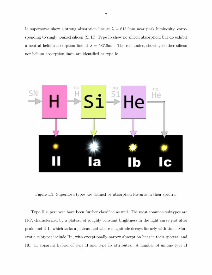
The physical nature of supernovae is perhaps best elucidated by the “guest star” of
1054 C.E., and the clues it has left behind. Chinese and Arab records of the event were
precise enough that its position can be located in the constellation of Taurus, and observed
through modern telescopes. There we find two remarkable objects, the Crab Nebula and the
Crab Pulsar.
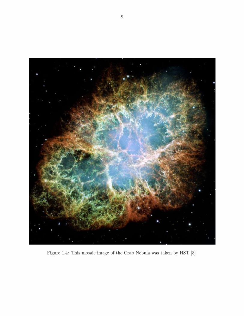
The Crab Nebula is a great cloud of gas, approximately 11 light years across. Time
series images of the nebula reveal that it is expanding at about 1500 kilometers per second;
extrapolating this expansion backward in time, we conclude that the nebula began expanding
from a compact, central region in the mid-11th century. Due to the strong coincidence in
time and position, it appears, therefore, that the Crab Nebula is a remnant of the event
observed on Earth in 1054 AD.
9
Figure 1.4: This mosaic image of the Crab Nebula was taken by HST [8]
10
Because the Crab Nebula is expanding in all directions, we infer that its speed of lateral
expansion is equal to its rate of radial expansion, measurable by the blue shift of spectral
lines. Dividing the nebula’s observed angular rate of expansion into the inferred actual speed
of expansion, the distance from Earth to the Crab Nebula can be calculated as about 6500
light years. To produce the bright light source described in historical records at such a great
distance, the 1054 AD event must have been a supernova.
The Crab Pulsar, discovered in 1965 [9], is a compact object located at the origin of
the Crab Nebula’s expansion. It is an optical pulsar, pulsating once every 33 milliseconds,
and also emits radiation at wavelengths ranging from radio to gamma rays. The pulsar is
particularly bright in x-ray wavelengths. The very rapid changes in the pulsar’s luminosity
require that it must be very compact, since light can only traverse about 10,000 kilometers
in one pulsation period, the source can be no larger.
Some thirty years before the Crab Pulsar’s discovery, a theory of stellar collapse was
proposed, predicting that massive stars would end their lives in supernovae [10]. According
to the theory, after a star has exhausted most of its hydrogen fuel, it lacks the heat and
radiation pressure to support its weight against gravitational collapse. For stars of ordinary
mass, the collapse is halted by the pressure of electron degeneracy, resulting in a white dwarf
star.
However, in more massive stars, electron degeneracy pressure is not strong enough to
resist gravity; electrons are under such intense gravitational pressure that they recombine
with protons to form neutrons, the inverse of nuclear beta decay. Removal of electrons due to
recombination lets the stellar core contract further, accelerating the recombination process
in a runaway chain reaction. In a matter of seconds, all the core’s electrons are consumed,
and the remaining core nucleons collapse in near free fall, followed by the outer layers of the
star.
The collapse continues until the stellar core approaches the density of nuclear matter, at
which time neutron degeneracy pressure becomes the dominant force. Once the core collapse
11
is halted, infalling matter from the outer layers of the star strikes the core and rebounds, cre-
ating an outward shock wave of enormous energy. This rebound shock propagates outward,
accelerating nearly all the mass of the star to escape velocity, leaving only the bare, neutron
core [10]. The energetic shockwave, and the radiation it produces, appear as a supernova to
distant observers.
The core collapse theory accounts for many features of the Crab Nebula. The initial
explosion corresponds to the supernova observed in 1054 AD, and the nebula is the expanding
remnant of the expelled outer layers of the star. The Crab Pulsar is then explained as the
remaining neutron star, pulsing due to its extremely rapid rotation. Such rapid rotation is
expected when a stellar core of typical angular momentum contracts to an object only a few
kilometers across.
Since the Crab Pulsar’s discovery, many other pulsars have been identified, many sur-
rounded by expanding, gaseous nebulae. The core collapse theory of supernovae is well
supported by evidence, though it does not fit well with one particular class of supernovae,
those of type Ia (SNIa). First, no pulsar is found in the remnant of any SNIa. Second, some
SNIa occur in galaxies which have had little to no star formation activity for billions of years.
Because massive stars have short lifetimes, around 50 million years or less, the core collapse
theory cannot explain why so many SNIa are observed in galaxies where star formation is
long dormant.
The leading theory explaining type Ia supernova is the accretion of matter onto a white
dwarf from a nearby companion star. As more mass accumulates on the white dwarf, its
gravitational pressure eventually exceeds the electron degeneracy pressure. The white dwarf
collapses, raising its internal temperature and density enough to ignite nuclear fusion of
carbon and heavier elements. The heat released further increases the temperature and ac-
celerates fusion, resulting in an explosive, runaway nuclear burning of the entire star. The
burning of carbon and oxygen produces a large quantity of unstable 56Ni, the subsequent
radioactive decay of which governs the supernova’s declining luminosity. [11].
12
1.5 Star Formation and Stellar Evolution
The bulk of star formation is thought to occur in cold molecular clouds, collections of
interstellar gas and dust light years across, ranging from only a few solar masses to millions
of solar masses. They are called molecular clouds because much of their hydrogen is bound
up in H2 molecules. Many such clouds have been observed in the Milky Way, and in other
nearby galaxies, often with newly formed and still-forming stars embedded within.
The processes by which molecular clouds form, and by which stars nucleate within the
clouds, are not well understood. A number of competing star formation theories have been
formulated, however more data is required to test them. In particular, the stellar initial
mass function (IMF) is of key importance. The IMF specifies the probability density of
initial stellar masses; it is well measured for stars of ordinary mass, but not for stars of
exceptionally high or low mass. Low mass stars are very faint, whereas high mass stars
have very short lifetimes. Star surveys, therefore, tend to have very low statistics in both
categories, confounding attempts to accurately measure the IMF at either extreme.
Stellar evolution is better understood than star formation, and is well modeled by rel-
atively simple numerical simulations. Once a star has become sufficiently compact due to
self-gravity, hydrogen fusion ignites and the star rapidly moves to the main sequence, a
regime in which the star’s mass almost completely determines its temperature, luminosity
and internal structure. Most stars visible in the sky are in the main sequence phase of their
life, and their mass can be reliably inferred from the color of starlight we observe.
Low mass stars have relatively low core temperature and density, and therefore burn
their hydrogen fuel very slowly. Stars with mass less than about 0.87 M burn hydrogen so
slowly that none have had time to exhaust their core hydrogen supply within the current
age of the universe.
More massive stars exhaust their core hydrogen more rapidly, so that their main sequence
lifetime is approximately as follows [6]:
13
τms = (M
M)−2.5 × 10¹⁰yr (1.2)
Once a star’s core hydrogen is exhausted, it enters a period of instability powered by fusion
of helium and heavier elements, and by hydrogen outside the core. Stars in this phase undergo
drastic changes in their equilibrium size, including the giant and supergiant stellar classes,
and can undergo pulsations in which a large fraction of the stellar envelope is ejected into
space. For stars of approximately 8M and lower, these convulsions continue until the star
has ejected and/or burned enough matter that nuclear fusion cannot be sustained, neither
for hydrogen nor heavier elements. In the absence of fusion-generated heat and radiation
pressure, the star collapses under gravity to extreme density. The collapse is finally halted
by electron degeneracy pressure, when it becomes so dense that all the electron quantum
states in its gravitational potential well are occupied. These extremely compact and hot
stellar remnants are known as white dwarfs.
Stars with initial mass more than approximately 8M have a different fate. Even after
ejecting much of its mass in the later phases of life, the steller core is able to sustain fusion
of helium and heavier elements. The star first burns the carbon produced by helium fusion
to make oxygen, then burns the oxygen to make silicon, and finally burns the silicon to make
iron.
The formation of iron represents an end point in the thermonuclear synthesis of elements.
When two nuclei fuse to form an element lighter than iron, the binding energy of the system
increases, due to the attractive nuclear strong force between nucleons. According to the
liquid drop model of the nucleus, the fused nucleus has high binding energy because it has
less total surface area than the original two nuclei, analogous to surface tension in classical
liquids [7].
For larger nuclei, the coulomb repulsion of nuclear protons must be taken into account,
reducing the nuclear binding energy by a term proportional to Z2, where Z is the atomic
number. At Z = 26 (iron), the coulomb term in the nuclear binding energy overwhelms the
14
surface area contribution given by the liquid drop model, so the fusion of iron with other
nuclei does not increase nuclear binding energy [7]. Thus when iron accumulates in the
innermost regions of the core, it is unable to burn, i.e. it cannot undergo any exothermic
nuclear reaction either through fusion or fission.
If gravitational pressure is sufficient, however, the iron core does become susceptible to an
endothermic nuclear reaction, the recombination of electrons and protons to form neutrons,
producing neutrinos as a byproduct. Once this reaction begins, the consumption of electrons
begins reducing the degeneracy pressure that supports the star. This allows the star to
contract, increasing gravitational pressure in the core and accelerating the recombination
process. The result is a runaway reaction, consuming all available electrons in the course of
a few seconds. The sudden recombination of electrons and protons produces a concentrated
burst of neutrinos; a core collapse supernova is actually more luminous in neutrinos than in
photons, though of course the neutrino radiation is far more difficult to detect. Hence core
collapse supernovae are less optically luminous than thermonuclear supernovae, even though
the total energy emitted is comparable for both supernova types.
The remaining core, now consisting entirely of neutrons, collapses under gravity until
halted by neutron degeneracy pressure, at which point it has reached the density of an
atomic nucleus. The surrounding stellar material first falls inward, then rebounds from the
neutron core when the collapse is halting, resulting in an outward propagating shock wave.
Once the shock breaks the visible surface of the star, a core collapse supernova has begun.
Over the course of the next few weeks, the expanding stellar envelope expands, first becoming
orders of magnitude brighter than the progenitor star, then gradually dimming as the ejecta
cools to interstellar temperatures.
15
1.6 Motivation for Measuring Core Collapse Rates
CCSN progenitors, stars massive enough to produce core collapse supernovae, have very
brief lives on astronomical time scales. At the lower bound of CCSN progenitor mass,
8 ± 1M, the star’s expected main sequence lifetime is 55+22−14Myr; more massive stars will
have even shorter lifetimes. Therefore, if we observe light from a core collapse supernova in
some past era of cosmic history, we know that its progenitor star formed within the preceding
55 million years or thereabouts. The bulk of the SDSS-II CCSN sample are observed at
redshifts near (z ≈ 0.1), where we see events that occurred about 1.4Gyr ago. Thus if we
use CCSN events as tracers of massive star formation, the time of core collapse lags the time
of star formation by less than 4%. By measuring the CCSN volumetric rate as a function of
time, we probe the star formation history of the universe.
Measuring the CCSN rate history of the universe is also useful to other measurements
where CCSN act as a background, contaminating the primary signal under study. Cos-
mology studies based on type Ia supernovae are in this category; some CCSN have light
curves superficially similar to SNIa, but do not obey the SNIa stretch-luminosity relation.
A CCSN rate measurement provides a quantitative basis for estimating the uncertainty in
SNIa cosmology results due to CCSN contamination. Neutrinos produced by CCSN also
may contaminate experiments searching for neutrinos from other sources, such as primordial
cosmic neutrinos. A more accurate CCSN rate measurement allows better subtraction of the
CCSN neutrino background.
The CCSN rate may also be compared to other star formation indicators, to better
understand differences between CCSN progenitor stars and the general stellar population.
Furthermore, a comparison of the CCSN rate to the overall star formation rate could reveal
more precisely the mass threshold between CCSN progenitors and white dwarf progenitors,
if the stellar initial mass function can be measured accurately by other means.
16
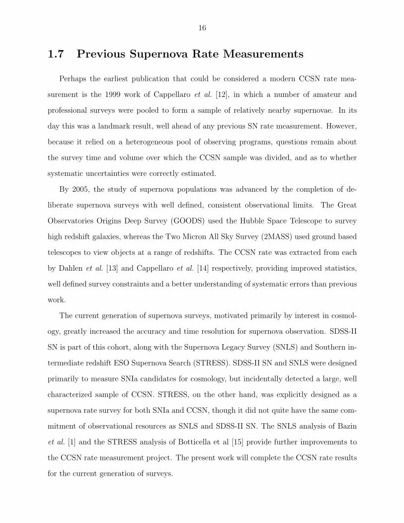
1.7 Previous Supernova Rate Measurements
Perhaps the earliest publication that could be considered a modern CCSN rate mea-
surement is the 1999 work of Cappellaro et al. [12], in which a number of amateur and
professional surveys were pooled to form a sample of relatively nearby supernovae. In its
day this was a landmark result, well ahead of any previous SN rate measurement. However,
because it relied on a heterogeneous pool of observing programs, questions remain about
the survey time and volume over which the CCSN sample was divided, and as to whether
systematic uncertainties were correctly estimated.
By 2005, the study of supernova populations was advanced by the completion of de-
liberate supernova surveys with well defined, consistent observational limits. The Great
Observatories Origins Deep Survey (GOODS) used the Hubble Space Telescope to survey
high redshift galaxies, whereas the Two Micron All Sky Survey (2MASS) used ground based
telescopes to view objects at a range of redshifts. The CCSN rate was extracted from each
by Dahlen et al. [13] and Cappellaro et al. [14] respectively, providing improved statistics,
well defined survey constraints and a better understanding of systematic errors than previous
work.
The current generation of supernova surveys, motivated primarily by interest in cosmol-
ogy, greatly increased the accuracy and time resolution for supernova observation. SDSS-II
SN is part of this cohort, along with the Supernova Legacy Survey (SNLS) and Southern in-
termediate redshift ESO Supernova Search (STRESS). SDSS-II SN and SNLS were designed
primarily to measure SNIa candidates for cosmology, but incidentally detected a large, well
characterized sample of CCSN. STRESS, on the other hand, was explicitly designed as a
supernova rate survey for both SNIa and CCSN, though it did not quite have the same com-
mitment of observational resources as SNLS and SDSS-II SN. The SNLS analysis of Bazin
et al. [1] and the STRESS analysis of Botticella et al [15] provide further improvements to
the CCSN rate measurement project. The present work will complete the CCSN rate results
for the current generation of surveys.
17
Chapter 2
The SDSS-II Supernova Survey
2.1 Astronomical Surveys
Traditionally, astronomical observations have tended to focus on individual targets, such
as a specific planet, star or galaxy. This is a sensible strategy, given that telescope time
has historically been scarce and that objects of interest occupy a tiny fraction of the sky’s
total observable area. This mode of observation still has great value, and will continue to be
practiced for the foreseeable future.
However, in recent times a second mode of observation has become viable, where large
regions of the sky are surveyed at once, capturing many object images simultaneously. Astro-
nomical surveys of this kind have been made possible by digital imaging technology. Because
the telescope images are represented electronically, it is possible to store and catalog a vast
database of images, even when the angular density of interesting objects is low. Also, elec-
tronic processing can compensate for the rotation of the Earth so that the telescope need
not track the apparent motion of the stars across the sky, a technique known as drift scan
imaging.
With the use of drift scan imaging and digital image processing, large sky surveys can now
be conducted at a reasonable cost, and the volume of astronomical survey data generated is
18
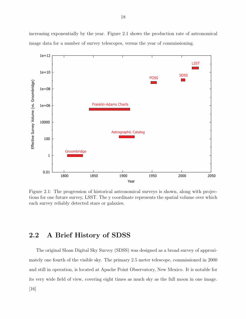
increasing exponentially by the year. Figure 2.1 shows the production rate of astronomical
image data for a number of survey telescopes, versus the year of commissioning.
0.01
1
100
10000
1e+06
1e+08
1e+10
1e+12
1800 1850 1900 1950 2000 2050
Effect
ive S
urv
ey
Volu
me (
vs. G
room
bridge)
Year
Groombridge
Astrographic Catalog
Franklin-Adams Charts
POSS SDSS
LSST
Figure 2.1: The progression of historical astronomical surveys is shown, along with projec-tions for one future survey, LSST. The y coordinate represents the spatial volume over whicheach survey reliably detected stars or galaxies.
2.2 A Brief History of SDSS
The original Sloan Digital Sky Survey (SDSS) was designed as a broad survey of approxi-
mately one fourth of the visible sky. The primary 2.5 meter telescope, commissioned in 2000
and still in operation, is located at Apache Point Observatory, New Mexico. It is notable for
its very wide field of view, covering eight times as much sky as the full moon in one image.
[16]
19
The SDSS telescope uses a large-format, 120-megapixel mosaic CCD camera to capture
five images simultaneously, each in a separate optical band [17]. The five optical bands
imaged by SDSS comprise the ’SDSS filter system’, which has since been adopted by a
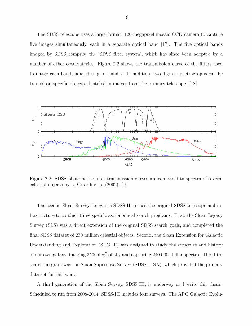
number of other observatories. Figure 2.2 shows the transmission curve of the filters used
to image each band, labeled u, g, r, i and z. In addition, two digital spectrographs can be
trained on specific objects identified in images from the primary telescope. [18]
Figure 2.2: SDSS photometric filter transmission curves are compared to spectra of severalcelestial objects by L. Girardi et al (2002). [19]
The second Sloan Survey, known as SDSS-II, reused the original SDSS telescope and in-
frastructure to conduct three specific astronomical search programs. First, the Sloan Legacy
Survey (SLS) was a direct extension of the original SDSS search goals, and completed the
final SDSS dataset of 230 million celestial objects. Second, the Sloan Extension for Galactic
Understanding and Exploration (SEGUE) was designed to study the structure and history
of our own galaxy, imaging 3500 deg2 of sky and capturing 240,000 stellar spectra. The third
search program was the Sloan Supernova Survey (SDSS-II SN), which provided the primary
data set for this work.
A third generation of the Sloan Survey, SDSS-III, is underway as I write this thesis.
Scheduled to run from 2008-2014, SDSS-III includes four surveys. The APO Galactic Evolu-
20
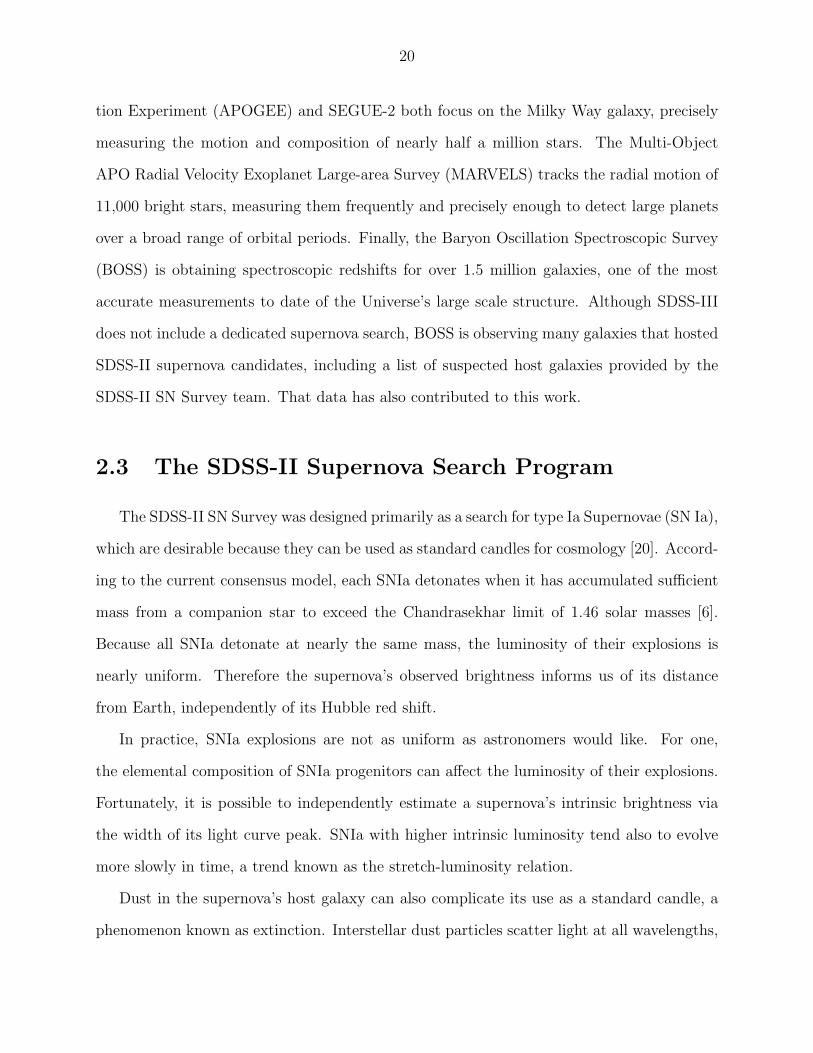
tion Experiment (APOGEE) and SEGUE-2 both focus on the Milky Way galaxy, precisely
measuring the motion and composition of nearly half a million stars. The Multi-Object
APO Radial Velocity Exoplanet Large-area Survey (MARVELS) tracks the radial motion of
11,000 bright stars, measuring them frequently and precisely enough to detect large planets
over a broad range of orbital periods. Finally, the Baryon Oscillation Spectroscopic Survey
(BOSS) is obtaining spectroscopic redshifts for over 1.5 million galaxies, one of the most
accurate measurements to date of the Universe’s large scale structure. Although SDSS-III
does not include a dedicated supernova search, BOSS is observing many galaxies that hosted
SDSS-II supernova candidates, including a list of suspected host galaxies provided by the
SDSS-II SN Survey team. That data has also contributed to this work.
2.3 The SDSS-II Supernova Search Program
The SDSS-II SN Survey was designed primarily as a search for type Ia Supernovae (SN Ia),
which are desirable because they can be used as standard candles for cosmology [20]. Accord-
ing to the current consensus model, each SNIa detonates when it has accumulated sufficient
mass from a companion star to exceed the Chandrasekhar limit of 1.46 solar masses [6].
Because all SNIa detonate at nearly the same mass, the luminosity of their explosions is
nearly uniform. Therefore the supernova’s observed brightness informs us of its distance
from Earth, independently of its Hubble red shift.
In practice, SNIa explosions are not as uniform as astronomers would like. For one,
the elemental composition of SNIa progenitors can affect the luminosity of their explosions.
Fortunately, it is possible to independently estimate a supernova’s intrinsic brightness via
the width of its light curve peak. SNIa with higher intrinsic luminosity tend also to evolve
more slowly in time, a trend known as the stretch-luminosity relation.
Dust in the supernova’s host galaxy can also complicate its use as a standard candle, a
phenomenon known as extinction. Interstellar dust particles scatter light at all wavelengths,
21
but scatter short, blue wavelengths most strongly. The effect is to reduce the supernova’s
apparent brightness, and to redden its apparent color.
The SDSS-II SN Survey, like other modern supernova studies, attacks problems of intrin-
sic luminosity variation and extinction with a detailed empirical model known as MLCS[21].
MLCS uses a multi-parameter warp to fit a candidate to a set of canonical SNIa templates,
finding the best fit distance modulus, extinction parameter (AV ) and SNIa stretch parameter
(∆). For most SNIa, MLCS has been shown to converge on results that match spectroscopic
confirmation with high confidence.
A second light curve program, SALT2 [22], was also applied to SDSS-II supernova light
curves, to assess the systematic effect of the fitting program itself on cosmology results.
SALT2 employs a similar, template-based approach to MLCS, but with the additional con-
straint that it minimizes the scatter of data points on the Hubble diagram. The initial
analysis, using only 2005 data, uncovered significant systematic differences in cosmology
results between MLCS and SALT2. However, work continues to reconcile the two models
through further analysis using the full three years of SDSS-II SN data. [21].
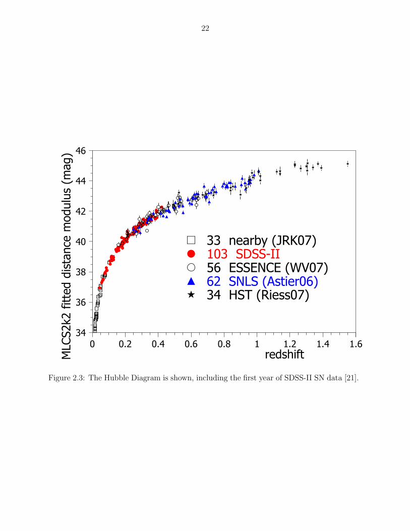
Prior to SDSS-II, supernova surveys for cosmology had concentrated on two extremes,
either wide angle surveys focusing on nearby galaxies, or deep, narrow surveys focusing on
the most distant galaxies. The intermediate region, from about z = 0.1 to 0.3, had sparse
SNIa data. The SDSS-II SN survey was specifically designed to study this redshift desert’,
and was quite successful in doing so. Figure 2.3 shows the Hubble diagram, a logarithmic
plot of distance versus redshift, combining SDSS-II SN data with other surveys.
Unlike most galaxies, supernovae change rapidly, with significant changes in brightness
on the scale of weeks or even days. Therefore, to properly observe supernovae requires a
shorter cadence, the time between images of the same sky region, compared to a galaxy
survey. For the SDSS-II SN Survey, a 300 deg2 region of sky, designated ’Stripe 82’, was
targeted for imaging once every two days; however, viewing conditions only allowed imaging
of the entire stripe once every four days, on average.
22
34
36
38
40
42
44
46
0 0.2 0.4 0.6 0.8 1 1.2 1.4 1.6redshift M
LCS2k2
fitte
d d
ista
nce
modulu
s (m
ag)
33 nearby (JRK07)103 SDSS-II56 ESSENCE (WV07)62 SNLS (Astier06)34 HST (Riess07)
Figure 2.3: The Hubble Diagram is shown, including the first year of SDSS-II SN data [21].
23
To detect supernovae within the search region, images from each night were first compared
to a template image of the same region of the sky. Any part of the image differing significantly
from the template was selected for further analysis, as it might indicate a distant object
whose brightness is variable on a time scale of days. To reduce the volume of data processed,
a catalog of known quasars, variable stars and active galactic nuclei (AGNs) was used to
exclude variable objects that are known not to be supernovae. Also, most objects within
the solar system are rejected by software; their proper motion is so rapid that their position
shifts significantly in the few minutes between g, r and i camera exposures.
The remaining variable objects were forwarded to a team of human scanners within the
collaboration. Images of each object were presented to one or more scanners, who registered
their judgment on whether the object might be a supernova. Many objects that show
image differences from night to night are not supernovae, such as asteroids, bright stars and
telescope artifacts. Also, when a variable object was detected in more than one year of
observation, it was excluded from the sample, as supernovae are very unlikely to be active
over such a long period of time. As the survey progressed, exclusion of these non-supernovae
became increasingly automated, so that a greater fraction of objects forwarded to human
scanners were subsequently identified as possible supernovae.
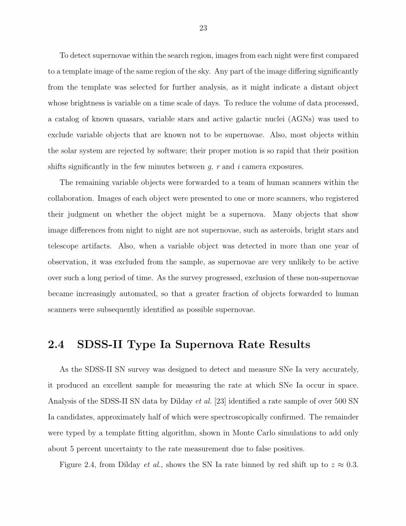
2.4 SDSS-II Type Ia Supernova Rate Results
As the SDSS-II SN survey was designed to detect and measure SNe Ia very accurately,
it produced an excellent sample for measuring the rate at which SNe Ia occur in space.
Analysis of the SDSS-II SN data by Dilday et al. [23] identified a rate sample of over 500 SN
Ia candidates, approximately half of which were spectroscopically confirmed. The remainder
were typed by a template fitting algorithm, shown in Monte Carlo simulations to add only
about 5 percent uncertainty to the rate measurement due to false positives.
Figure 2.4, from Dilday et al., shows the SN Ia rate binned by red shift up to z ≈ 0.3.
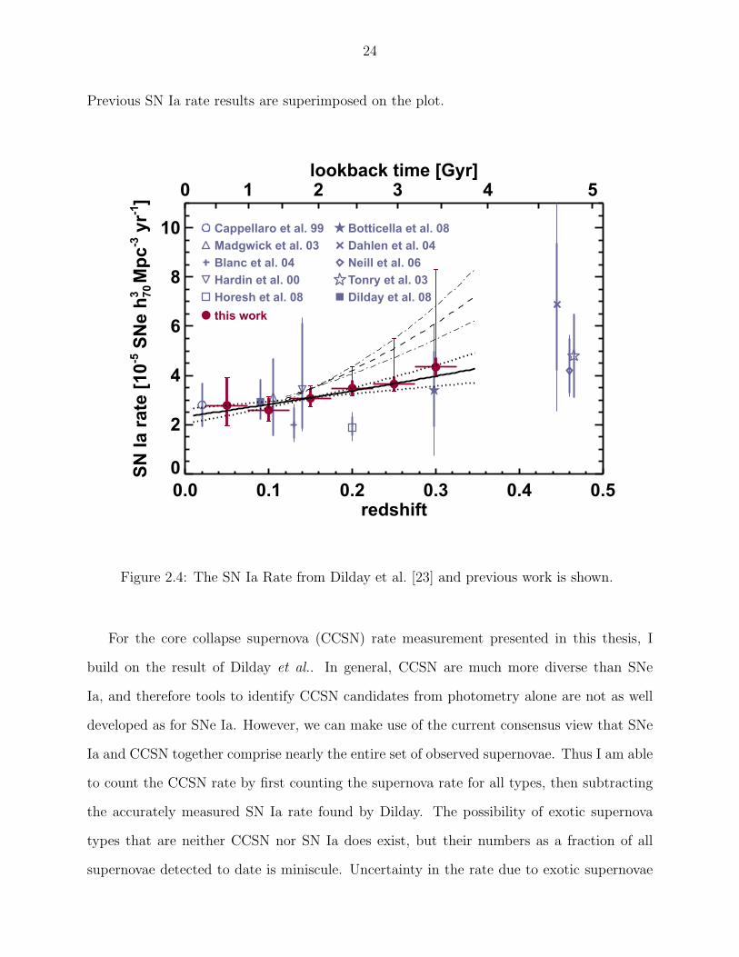
24
Previous SN Ia rate results are superimposed on the plot.
0.0 0.1 0.2 0.3 0.4 0.5redshift
0
2
4
6
8
10
SN
Ia r
ate
[10
-5 S
Ne h
70
3 M
pc
-3 y
r-1]
0 1 2 3 4 5lookback time [Gyr]
Cappellaro et al. 99
Madgwick et al. 03
Blanc et al. 04
Hardin et al. 00
Horesh et al. 08
Botticella et al. 08
Dahlen et al. 04
Neill et al. 06
Tonry et al. 03
Dilday et al. 08
this work
Figure 2.4: The SN Ia Rate from Dilday et al. [23] and previous work is shown.
For the core collapse supernova (CCSN) rate measurement presented in this thesis, I
build on the result of Dilday et al.. In general, CCSN are much more diverse than SNe
Ia, and therefore tools to identify CCSN candidates from photometry alone are not as well
developed as for SNe Ia. However, we can make use of the current consensus view that SNe
Ia and CCSN together comprise nearly the entire set of observed supernovae. Thus I am able
to count the CCSN rate by first counting the supernova rate for all types, then subtracting
the accurately measured SN Ia rate found by Dilday. The possibility of exotic supernova
types that are neither CCSN nor SN Ia does exist, but their numbers as a fraction of all
supernovae detected to date is miniscule. Uncertainty in the rate due to exotic supernovae

25
is negligible compared to other sources of error.
2.5 BOSS Object Identifications and Redshift Mea-
surements
At the beginning of the SDSS-III BOSS project, the SDSS-II Supernova Survey team
compiled a list of suggested targets for BOSS. The suggested targets were a complete list
of galaxies matching two criteria: that the galaxy is nearest to a supernova candidate in
angular distance, and also nearest in isophotal distance. Isophotal distance measures the
candidate’s distance from the galaxy center, as a fraction of the galaxy’s size along the
galaxy-candidate axis. When a galaxy is nearest to a candidate in both angular and isophotal
distance, confidence is high that it is the galaxy in which the supernova candidate actually
occurred. [21]
Fortunately for this work, the BOSS collaboration scheduled the recommended SDSS-II
targets very early in their observation plan. Many of the recommended targets could not
be observed due to technical and observational constraints; however, BOSS was still able to
collect spectra for 2,458 targets. BOSS discovered that some of the targets were variable
stars or quasars, which likely means that the variable light source observed by SDSS-II was
not a supernova at all. For the remainder, which appear to be typical, inactive galaxies, the
BOSS team measured redshifts using the spectrum analysis pipeline already developed for
their primary mission. [24]
26
Chapter 3
Rate Measurement Technique
3.1 Candidate Selection
The data analysis pipeline described in this section is not specific to my core collapse rate
measurement; it was designed to identify supernovae in general, and the set of supernova
candidates it generated has been used by all supernova-related work by the SDSS-II collab-
oration. Technical details of the pipeline, summarized below, are covered in the published
SDSS-II Supernova Survey Technical Summary [20].
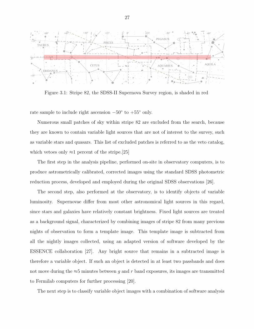
The SDSS-II SN data analysis pipeline is designed to identify supernova candidates among
the sequence of images of “stripe 82”, the survey’s designated region of sky. The full region
surveyed extends from right ascension (RA) −60 to +60, and from declination −1.25
to +1.25. It is a narrow strip of sky along the celestial equator, primarily located in the
constellations of Aquarius, Pisces and Cetus, with minor portions in Aquila, Taurus and
Eridanus, as shown in Figure 3.1.
Prior SDSS-II work, such as the SNIa rate measurement of Dilday et al. [25], has noted
systematic observational anomalies at the outermost edges of the stripe 82 RA range. Tem-
plates were not available for that region of the sky during the first year of observation, and
the calibration star catalog does not completely cover that region. Therefore, I restrict my
27
ERIDANUS
TAURUS
CETUS
PISCES
AQUARIUS AQUILA
PEGASUS
0° -15° -30°+30° -45° -60°+15°+45°+60°
0°
+15°
-15°
Figure 3.1: Stripe 82, the SDSS-II Supernova Survey region, is shaded in red
rate sample to include right ascension −50 to +55 only.
Numerous small patches of sky within stripe 82 are excluded from the search, because
they are known to contain variable light sources that are not of interest to the survey, such
as variable stars and quasars. This list of excluded patches is referred to as the veto catalog,
which vetoes only ≈1 percent of the stripe.[25]
The first step in the analysis pipeline, performed on-site in observatory computers, is to
produce astrometrically calibrated, corrected images using the standard SDSS photometric
reduction process, developed and employed during the original SDSS observations [26].
The second step, also performed at the observatory, is to identify objects of variable
luminosity. Supernovae differ from most other astronomical light sources in this regard,
since stars and galaxies have relatively constant brightness. Fixed light sources are treated
as a background signal, characterized by combining images of stripe 82 from many previous
nights of observation to form a template image. This template image is subtracted from
all the nightly images collected, using an adapted version of software developed by the
ESSENCE collaboration [27]. Any bright source that remains in a subtracted image is
therefore a variable object. If such an object is detected in at least two passbands and does
not move during the ≈5 minutes between g and r band exposures, its images are transmitted
to Fermilab computers for further processing [20].
The next step is to classify variable object images with a combination of software analysis
28
and human scanning. Some of the variable objects turn out not to be variable light sources at
all; they are just artifacts of the observation process. Diffraction spikes from telescope optics
can vary from one night to the next, and therefore be incorrectly flagged as variable objects.
The brightest stars can saturate the Sloan telescope’s camera CCDs, forming unpredictable
patterns in the resulting image data. Asteroids within our solar system move through the
field of view, and their change in position also appears as a difference versus the background
template. Initially, the survey relied on human eyes to visually scan each image and identify
these artifacts. Later, software routines were developed that filtered out most of the artifacts.
Objects passing the software checks were still scanned by human eyes, and still contained
a significant number of artifacts, though the volume of objects that required scanning was
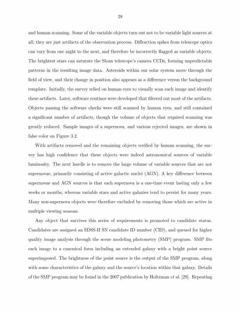
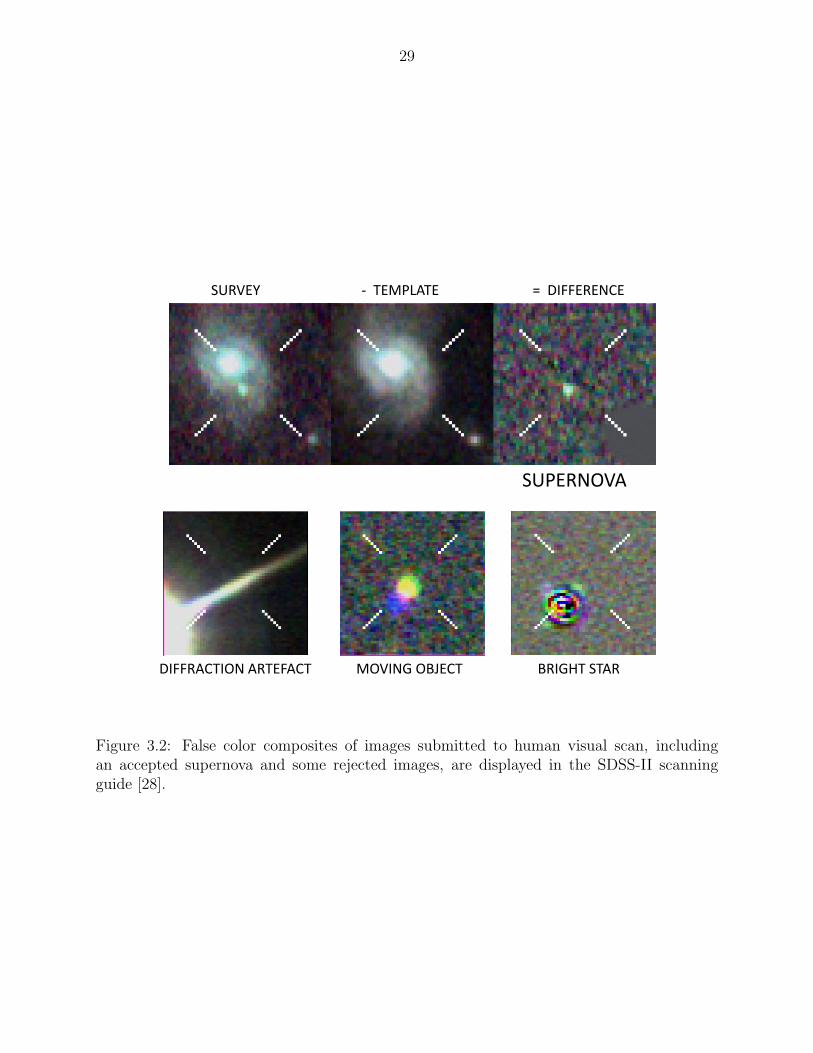
greatly reduced. Sample images of a supernova, and various rejected images, are shown in
false color on Figure 3.2.
With artifacts removed and the remaining objects verified by human scanning, the sur-
vey has high confidence that these objects were indeed astronomical sources of variable
luminosity. The next hurdle is to remove the large volume of variable sources that are not
supernovae, primarily consisting of active galactic nuclei (AGN). A key difference between
supernovae and AGN sources is that each supernova is a one-time event lasting only a few
weeks or months, whereas variable stars and active galaxies tend to persist for many years.
Many non-supernova objects were therefore excluded by removing those which are active in
multiple viewing seasons.
Any object that survives this series of requirements is promoted to candidate status.
Candidates are assigned an SDSS-II SN candidate ID number (CID), and queued for higher
quality image analysis through the scene modeling photometry (SMP) program. SMP fits
each image to a canonical form including an extended galaxy with a bright point source
superimposed. The brightness of the point source is the output of the SMP program, along
with some characteristics of the galaxy and the source’s location within that galaxy. Details
of the SMP program may be found in the 2007 publication by Holtzman et al. [29]. Repeating
29
SURVEY - TEMPLATE = DIFFERENCE
DIFFRACTION ARTEFACT MOVING OBJECT BRIGHT STAR
SUPERNOVA
Figure 3.2: False color composites of images submitted to human visual scan, includingan accepted supernova and some rejected images, are displayed in the SDSS-II scanningguide [28].
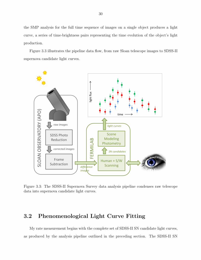
30
the SMP analysis for the full time sequence of images on a single object produces a light
curve, a series of time-brightness pairs representing the time evolution of the object’s light
production.
Figure 3.3 illustrates the pipeline data flow, from raw Sloan telescope images to SDSS-II
supernova candidate light curves.
SDSS PhotoReduction
FrameSubtractionSL
OA
N O
BSE
RV
ATO
RY
(AP
O)
raw images
corrected images
Human + S/W Scanning
Scene Modeling
Photometry
differenceimages
FER
MIL
AB
SN candidates
time
ligh
t fl
ux
light curves
Figure 3.3: The SDSS-II Supernova Survey data analysis pipeline condenses raw telescopedata into supernova candidate light curves.
3.2 Phenomenological Light Curve Fitting
My rate measurement begins with the complete set of SDSS-II SN candidate light curves,
as produced by the analysis pipeline outlined in the preceding section. The SDSS-II SN
31
Survey used relatively loose criteria for identifying a supernova candidate, followed by stricter
light curve quality criteria for the SNIa cosmology sample [21]. Of course, I do not apply the
cosmology SNIa requirements for my sample, because SNIa are not core collapse supernovae.
Therefore, the candidate set from which I begin includes a large number of variable objects
that are not supernovae, such as variable stars, quasars and other active galaxies, or perhaps
even novae within the Milky Way.
To separate supernovae from other variable object types, I employed the phenomeno-
logical light curve fitting method used by Bazin et al. in the Supernova Legacy Survey
(SNLS). [1] Bazin models observed supernova brightness in each passband as a function of
time using the parameterized formula:
f(t) = Ae−(
t−t0τF
)(1 + e
−(t−t0τR
))−1 (3.1)
The left hand side of Equation 3.1 measures supernova brightness as flux, i.e. power
received per unit area of the camera. The microjansky (µJy) is the unit of flux used by
SDSS-II, equal to 10−32 watts per square meter.
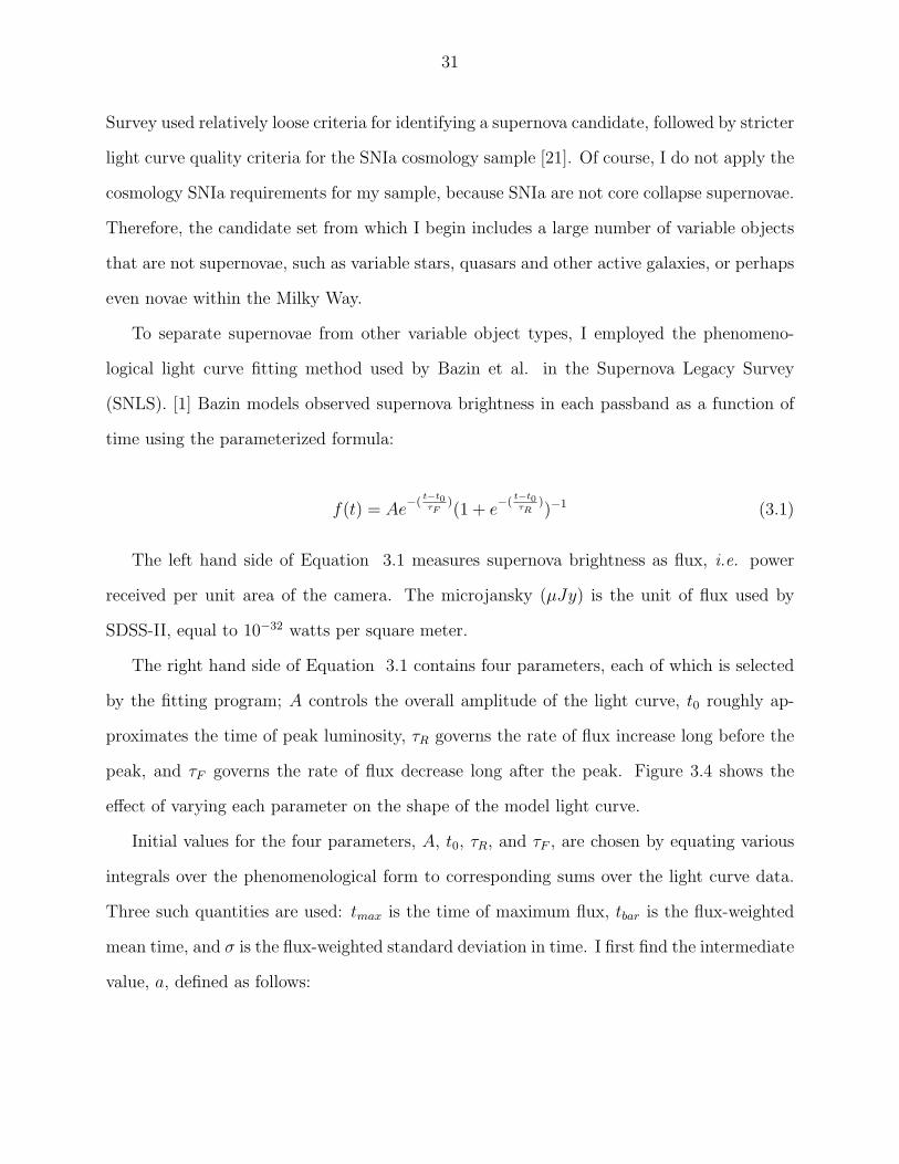
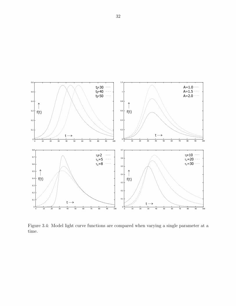
The right hand side of Equation 3.1 contains four parameters, each of which is selected
by the fitting program; A controls the overall amplitude of the light curve, t0 roughly ap-
proximates the time of peak luminosity, τR governs the rate of flux increase long before the
peak, and τF governs the rate of flux decrease long after the peak. Figure 3.4 shows the
effect of varying each parameter on the shape of the model light curve.
Initial values for the four parameters, A, t0, τR, and τF , are chosen by equating various
integrals over the phenomenological form to corresponding sums over the light curve data.
Three such quantities are used: tmax is the time of maximum flux, tbar is the flux-weighted
mean time, and σ is the flux-weighted standard deviation in time. I first find the intermediate
value, a, defined as follows:
32
0
0.1
0.2
0.3
0.4
0.5
0.6
0 10 20 30 40 50 60 70 80 90 100
t=500
t
f(t)
t=400
t=300
0
0.1
0.2
0.3
0.4
0.5
0.6
0.7
0 10 20 30 40 50 60 70 80 90 100
t
f(t)
tF=30tF=20t=10F
0
0.1
0.2
0.3
0.4
0.5
0.6
0.7
0.8
0 10 20 30 40 50 60 70 80 90 100
t
f(t)
tR=8tR=5t=2R
0
0.2
0.4
0.6
0.8
1
1.2
0 10 20 30 40 50 60 70 80 90 100
t
f(t)
A=2.0A=1.5A=1.0
Figure 3.4: Model light curve functions are compared when varying a single parameter at atime.
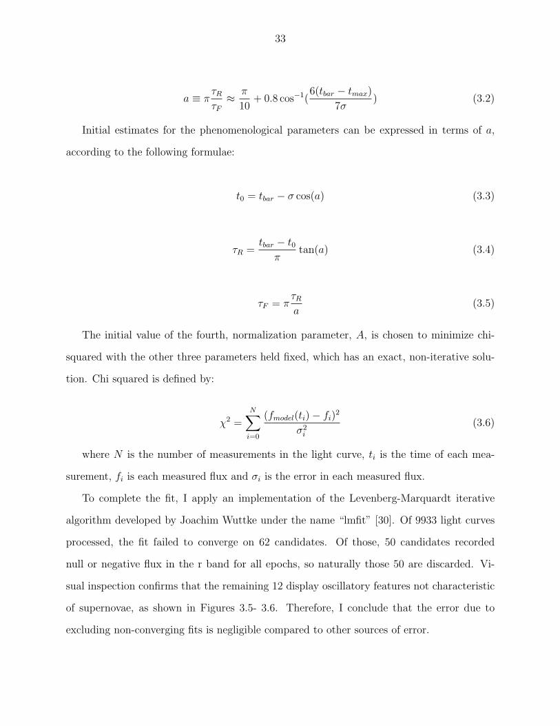
33
a ≡ πτRτF≈ π
10+ 0.8 cos−1(
6(tbar − tmax)
7σ) (3.2)
Initial estimates for the phenomenological parameters can be expressed in terms of a,
according to the following formulae:
t0 = tbar − σ cos(a) (3.3)
τR =tbar − t0
πtan(a) (3.4)
τF = πτRa
(3.5)
The initial value of the fourth, normalization parameter, A, is chosen to minimize chi-
squared with the other three parameters held fixed, which has an exact, non-iterative solu-
tion. Chi squared is defined by:
χ2 =N∑
i=0
(fmodel(ti)− fi)2
σ2i
(3.6)
where N is the number of measurements in the light curve, ti is the time of each mea-
surement, fi is each measured flux and σi is the error in each measured flux.
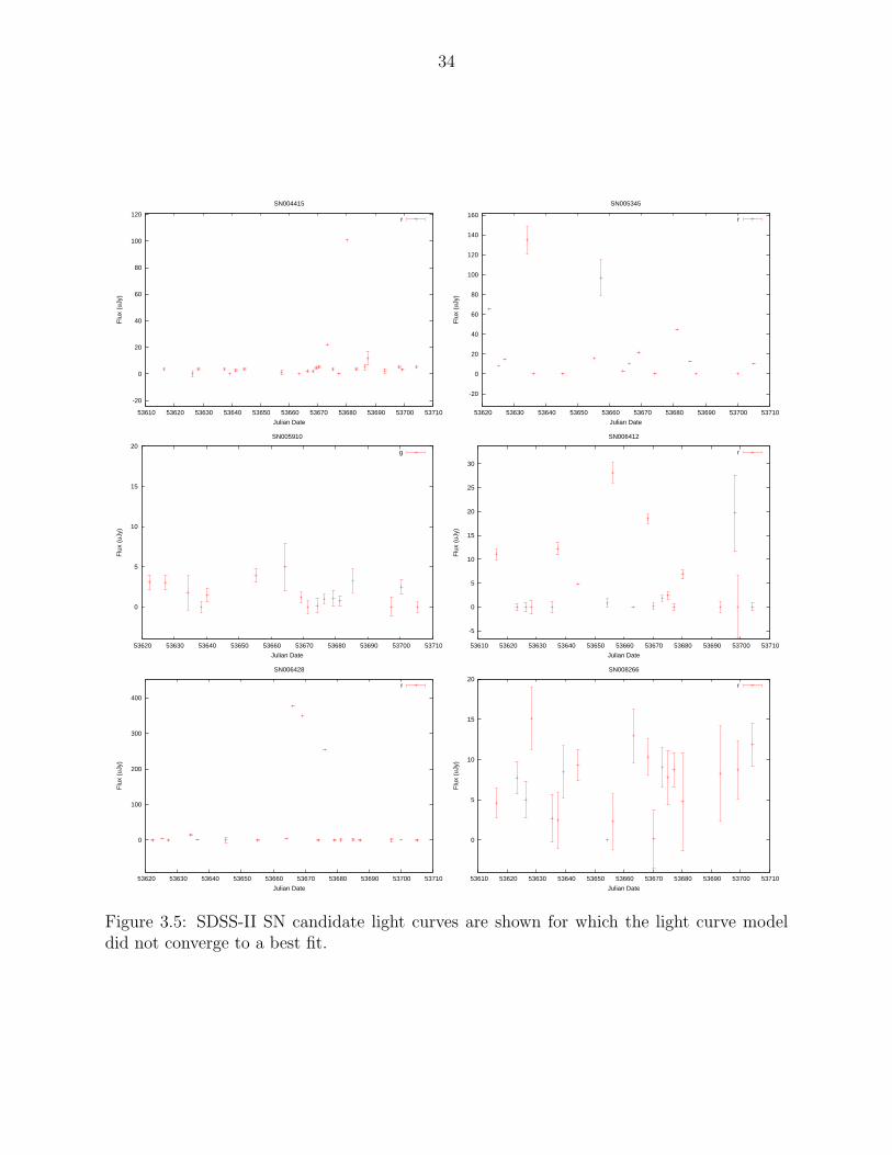
To complete the fit, I apply an implementation of the Levenberg-Marquardt iterative
algorithm developed by Joachim Wuttke under the name “lmfit” [30]. Of 9933 light curves
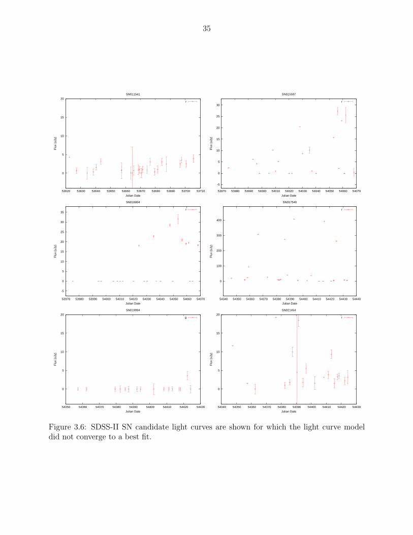
processed, the fit failed to converge on 62 candidates. Of those, 50 candidates recorded
null or negative flux in the r band for all epochs, so naturally those 50 are discarded. Vi-
sual inspection confirms that the remaining 12 display oscillatory features not characteristic
of supernovae, as shown in Figures 3.5- 3.6. Therefore, I conclude that the error due to
excluding non-converging fits is negligible compared to other sources of error.
34
-20
0
20
40
60
80
100
120
53610 53620 53630 53640 53650 53660 53670 53680 53690 53700 53710
Flu
x (u
Jy)
Julian Date
SN004415
r
-20
0
20
40
60
80
100
120
140
160
53620 53630 53640 53650 53660 53670 53680 53690 53700 53710
Flu
x (u
Jy)
Julian Date
SN005345
r
0
5
10
15
20
53620 53630 53640 53650 53660 53670 53680 53690 53700 53710
Flu
x (u
Jy)
Julian Date
SN005910
g
-5
0
5
10
15
20
25
30
53610 53620 53630 53640 53650 53660 53670 53680 53690 53700 53710
Flu
x (u
Jy)
Julian Date
SN006412
r
0
100
200
300
400
53620 53630 53640 53650 53660 53670 53680 53690 53700 53710
Flu
x (u
Jy)
Julian Date
SN006428
r
0
5
10
15
20
53610 53620 53630 53640 53650 53660 53670 53680 53690 53700 53710
Flu
x (u
Jy)
Julian Date
SN008266
r
Figure 3.5: SDSS-II SN candidate light curves are shown for which the light curve modeldid not converge to a best fit.
35
0
5
10
15
20
53620 53630 53640 53650 53660 53670 53680 53690 53700 53710
Flu
x (u
Jy)
Julian Date
SN011541
r
-5
0
5
10
15
20
25
30
53970 53980 53990 54000 54010 54020 54030 54040 54050 54060 54070
Flu
x (u
Jy)
Julian Date
SN015597
r
-5
0
5
10
15
20
25
30
35
53970 53980 53990 54000 54010 54020 54030 54040 54050 54060 54070
Flu
x (u
Jy)
Julian Date
SN016004
r
0
100
200
300
400
54340 54350 54360 54370 54380 54390 54400 54410 54420 54430 54440
Flu
x (u
Jy)
Julian Date
SN017540
r
0
5
10
15
20
54350 54360 54370 54380 54390 54400 54410 54420 54430
Flu
x (u
Jy)
Julian Date
SN019994
g
0
5
10
15
20
54340 54350 54360 54370 54380 54390 54400 54410 54420 54430
Flu
x (u
Jy)
Julian Date
SN021454
r
Figure 3.6: SDSS-II SN candidate light curves are shown for which the light curve modeldid not converge to a best fit.
36
3.3 Removal of Core Collapse Impostors
The phenomenological supernova model adapted from Bazin et al. can be fit to virtually
any light curve; however, the fit will be poor for light curves without a clear, dominant peak.
To measure the quality of the fit, I again follow the method of Bazin et al. [1] by fitting
a second, trivial model to each light curve, which is just the best-fit constant flux. The
chi-squared for this trivial fit can be solved exactly, without iteration.
When the trivial, constant flux fit has a chi-squared comparable to the chi-squared for
the model fit, the object either is not a supernova, or the data is too noisy to identify it as
a supernova. In either case, I remove such objects from the rate sample. The model and
constant flux chi-squared can be directly compared, even though the model has three more
degrees of freedom in its parameters, because both are fitted to the same number of data
points, and that number is much greater than the number of free parameters. To quantify
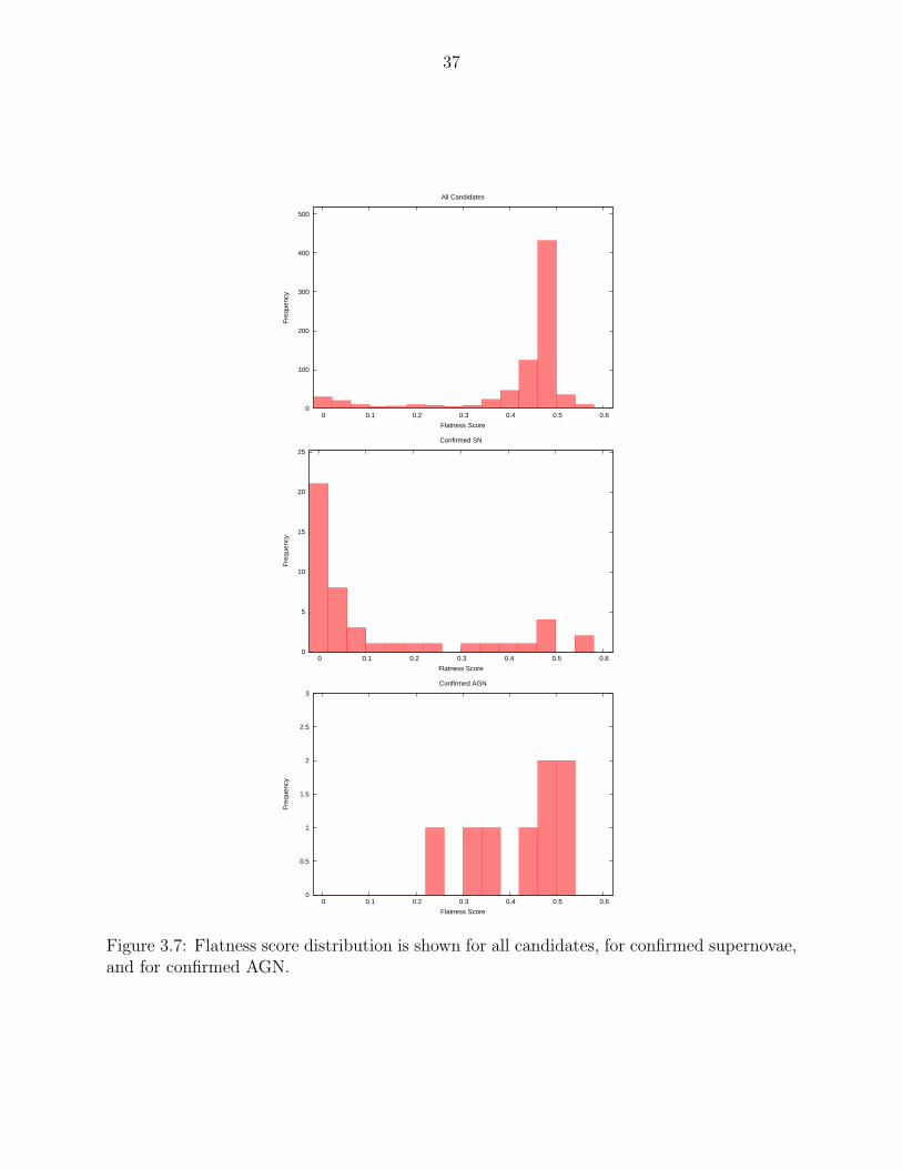
this comparison, I assign each light curve a flatness score, Λ, defined by:
Λ ≡ χ2model
χ2model + χ2
const
(3.7)
The value of Λ ranges from zero for the best measured, confirmed supernovae, to one for
light curves that show no supernova features. Figure 3.7 shows the distribution of Λ for all
SDSS-II SN candidates. It is is bimodal, with a large peak near Λ = 0.5, and a smaller peak
near Λ = 0.
To test the correlation between flatness score and object type, I examine the Λ distri-
bution for two candidate subsamples: core collapse supernovae and active galaxies, both
of which have been confirmed through spectroscopic analysis, as described by Sako et al.
(2008) [31]. The middle plot in Figure 3.7 shows that confirmed CCSN are concentrated near
Λ = 0, while the bottom plot shows that confirmed AGN are concentrated near Λ = 0.5.
To remove the bulk of the non-supernovae from the rate sample, the rate calculation pro-
gram calculates a cutoff, Λc, above which candidates are excluded. The program calculates
37
0
100
200
300
400
500
0 0.1 0.2 0.3 0.4 0.5 0.6
Fre
quen
cy
Flatness Score
All Candidates
0
5
10
15
20
25
0 0.1 0.2 0.3 0.4 0.5 0.6
Fre
quen
cy
Flatness Score
Confirmed SN
0
0.5
1
1.5
2
2.5
3
0 0.1 0.2 0.3 0.4 0.5 0.6
Fre
quen
cy
Flatness Score
Confirmed AGN
Figure 3.7: Flatness score distribution is shown for all candidates, for confirmed supernovae,and for confirmed AGN.
38
Λc by comparing the Λ distribution of the confirmed supernovae to that of the confirmed
non-supernovae. In both the confirmed CCSN and confirmed AGN subsamples, there are
some outlying light curves with unusually high or low Λ. The fraction of confirmed CCSN
with Λ > Λc estimates the rate of false negatives, i.e. the fraction of actual CCSN that will
be removed from the rate sample at that value of Λc. Likewise, the fraction of confirmed
AGN with Λ < Λc estimates the rate of false positives, i.e. the fraction of SN impostors that
will be included in the rate sample at that value of Λc.
The total number of candidates in the sample volume is known, up to detection efficiency,
and each candidate has a flatness score. Therefore, for any choice of the cutoff value, Λc, the
number of candidates below Λc (likely supernovae) and the number above Λc (likely AGN)
are also known. Likewise, I estimate the number of false positives and false negatives as
follows:
false positives = (confirmed AGN with Λ < Λc
all confirmed AGN)× candidates with Λ > Λc (3.8)
false negatives = (confirmed CCSN with Λ > Λc
all confirmed CCSN)× candidates with Λ < Λc (3.9)
The selected value, Λc = 0.354, is that at which the estimated number of false positives
is equal to the estimated number of false negatives, implying that the correction to the
supernova count for misidentification is zero. The rate of false positives and false negatives
do, however, contribute to sources of systematic error. A selection of light curves excluded
by the flatness score requirement is shown in Figures 3.8- 3.9.
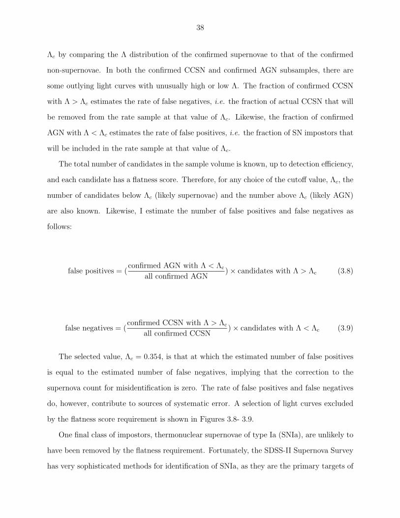
One final class of impostors, thermonuclear supernovae of type Ia (SNIa), are unlikely to
have been removed by the flatness requirement. Fortunately, the SDSS-II Supernova Survey
has very sophisticated methods for identification of SNIa, as they are the primary targets of
39
-20
0
20
40
60
80
100
53620 53630 53640 53650 53660 53670 53680 53690 53700 53710
Flu
x (u
Jy)
Julian Date
SN001552
DATAMODEL FITTRIVIAL FIT
-10
0
10
20
30
40
50
53620 53630 53640 53650 53660 53670 53680 53690 53700 53710
Flu
x (u
Jy)
Julian Date
SN005490
DATAMODEL FITTRIVIAL FIT
-20
0
20
40
60
80
100
53620 53630 53640 53650 53660 53670 53680 53690 53700 53710
Flu
x (u
Jy)
Julian Date
SN005866
DATAMODEL FITTRIVIAL FIT
-20
0
20
40
60
80
100
120
53970 53980 53990 54000 54010 54020 54030 54040 54050 54060 54070
Flu
x (u
Jy)
Julian Date
SN012819
DATAMODEL FITTRIVIAL FIT
0
5
10
15
20
53970 53980 53990 54000 54010 54020 54030 54040 54050 54060 54070
Flu
x (u
Jy)
Julian Date
SN012857
DATAMODEL FITTRIVIAL FIT
0
5
10
15
20
53970 53980 53990 54000 54010 54020 54030 54040 54050 54060 54070
Flu
x (u
Jy)
Julian Date
SN012862
DATAMODEL FITTRIVIAL FIT
Figure 3.8: Above are examples of confirmed AGN light curves, with the best model fitplotted in green and the trivial, constant flux fit in blue. All these candidates were excludedby the flatness requirement.
40
0
5
10
15
20
53970 53980 53990 54000 54010 54020 54030 54040 54050 54060 54070
Flu
x (u
Jy)
Julian Date
SN013408
DATAMODEL FITTRIVIAL FIT
0
5
10
15
20
53970 53980 53990 54000 54010 54020 54030 54040 54050 54060 54070
Flu
x (u
Jy)
Julian Date
SN013827
DATAMODEL FITTRIVIAL FIT
-5
0
5
10
15
20
25
53970 53980 53990 54000 54010 54020 54030 54040 54050 54060 54070
Flu
x (u
Jy)
Julian Date
SN015396
DATAMODEL FITTRIVIAL FIT
0
5
10
15
20
53970 53980 53990 54000 54010 54020 54030 54040 54050 54060 54070
Flu
x (u
Jy)
Julian Date
SN016469
DATAMODEL FITTRIVIAL FIT
0
5
10
15
20
53970 53980 53990 54000 54010 54020 54030 54040 54050 54060 54070
Flu
x (u
Jy)
Julian Date
SN016754
DATAMODEL FITTRIVIAL FIT
0
5
10
15
20
54340 54350 54360 54370 54380 54390 54400 54410 54420 54430 54440
Flu
x (u
Jy)
Julian Date
SN018264
DATAMODEL FITTRIVIAL FIT
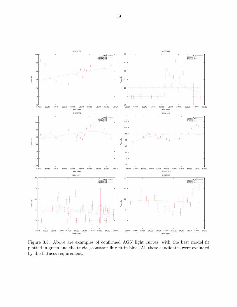
Figure 3.9: Above are examples of confirmed AGN light curves. All were excluded by theflatness requirement.
41
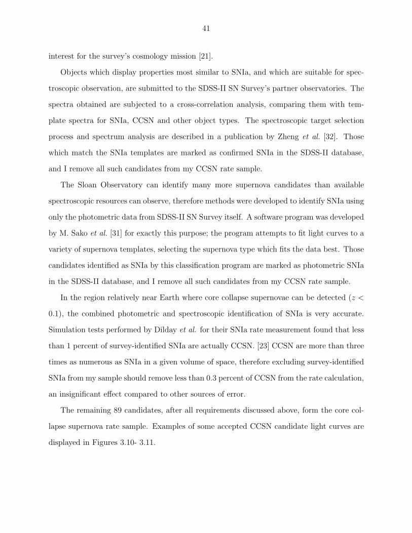
interest for the survey’s cosmology mission [21].
Objects which display properties most similar to SNIa, and which are suitable for spec-
troscopic observation, are submitted to the SDSS-II SN Survey’s partner observatories. The
spectra obtained are subjected to a cross-correlation analysis, comparing them with tem-
plate spectra for SNIa, CCSN and other object types. The spectroscopic target selection
process and spectrum analysis are described in a publication by Zheng et al. [32]. Those
which match the SNIa templates are marked as confirmed SNIa in the SDSS-II database,
and I remove all such candidates from my CCSN rate sample.
The Sloan Observatory can identify many more supernova candidates than available
spectroscopic resources can observe, therefore methods were developed to identify SNIa using
only the photometric data from SDSS-II SN Survey itself. A software program was developed
by M. Sako et al. [31] for exactly this purpose; the program attempts to fit light curves to a
variety of supernova templates, selecting the supernova type which fits the data best. Those
candidates identified as SNIa by this classification program are marked as photometric SNIa
in the SDSS-II database, and I remove all such candidates from my CCSN rate sample.
In the region relatively near Earth where core collapse supernovae can be detected (z <
0.1), the combined photometric and spectroscopic identification of SNIa is very accurate.
Simulation tests performed by Dilday et al. for their SNIa rate measurement found that less
than 1 percent of survey-identified SNIa are actually CCSN. [23] CCSN are more than three
times as numerous as SNIa in a given volume of space, therefore excluding survey-identified
SNIa from my sample should remove less than 0.3 percent of CCSN from the rate calculation,
an insignificant effect compared to other sources of error.
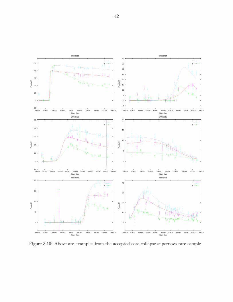
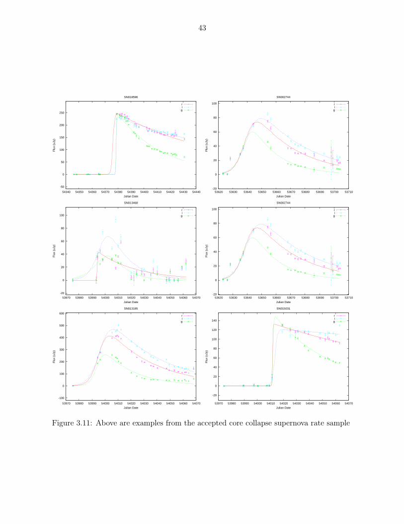
The remaining 89 candidates, after all requirements discussed above, form the core col-
lapse supernova rate sample. Examples of some accepted CCSN candidate light curves are
displayed in Figures 3.10- 3.11.
42
-10
0
10
20
30
40
50
53620 53630 53640 53650 53660 53670 53680 53690 53700 53710
Flu
x (u
Jy)
Julian Date
SN003818
ri
g
-5
0
5
10
15
20
25
30
35
40
53610 53620 53630 53640 53650 53660 53670 53680 53690 53700 53710
Flu
x (u
Jy)
Julian Date
SN010777
ri
g
-10
0
10
20
30
40
50
54340 54350 54360 54370 54380 54390 54400 54410 54420 54430 54440
Flu
x (u
Jy)
Julian Date
SN018700
ri
g
0
5
10
15
20
53620 53630 53640 53650 53660 53670 53680 53690 53700 53710
Flu
x (u
Jy)
Julian Date
SN002615
ri
g
0
5
10
15
20
53980 53990 54000 54010 54020 54030 54040 54050 54060 54070
Flu
x (u
Jy)
Julian Date
SN016087
ri
g
0
10
20
30
40
53610 53620 53630 53640 53650 53660 53670 53680 53690 53700 53710
Flu
x (u
Jy)
Julian Date
SN002793
ri
g
Figure 3.10: Above are examples from the accepted core collapse supernova rate sample.
43
-50
0
50
100
150
200
250
54340 54350 54360 54370 54380 54390 54400 54410 54420 54430 54440
Flu
x (u
Jy)
Julian Date
SN018596
ri
g
-20
0
20
40
60
80
100
53620 53630 53640 53650 53660 53670 53680 53690 53700 53710
Flu
x (u
Jy)
Julian Date
SN002744
ri
g
-20
0
20
40
60
80
100
53970 53980 53990 54000 54010 54020 54030 54040 54050 54060 54070
Flu
x (u
Jy)
Julian Date
SN013468
ri
g
-20
0
20
40
60
80
100
53620 53630 53640 53650 53660 53670 53680 53690 53700 53710
Flu
x (u
Jy)
Julian Date
SN002744
ri
g
-100
0
100
200
300
400
500
600
53970 53980 53990 54000 54010 54020 54030 54040 54050 54060 54070
Flu
x (u
Jy)
Julian Date
SN013195
ri
g
-20
0
20
40
60
80
100
120
140
53970 53980 53990 54000 54010 54020 54030 54040 54050 54060 54070
Flu
x (u
Jy)
Julian Date
SN015031
ri
g
Figure 3.11: Above are examples from the accepted core collapse supernova rate sample
44
3.4 Luminosity, Distance and Volume Measurement
I measure the distance to a supernova via the spectrum redshift of the supernova itself,
or of the galaxy in which it occurred. The preferred redshift measurements are those from
the supernova spectrum itself, although this data is only available for a small fraction of
candidates. More often, I use the redshift of the candidate’s apparent host galaxy as an esti-
mate of the supernova’s redshift. Fortunately, SDSS-III BOSS has provided a spectroscopic
redshift measurement for most of the host galaxies. The rest of the host galaxy redshifts are
estimated using the photometric redshift algorithm of the original Sloan survey [34]. Fig-
ure 3.12 displays the resulting redshift distribution of candidates in the CCSN rate sample.
Systematic error due to uncertainty in these photometric galaxy redshifts is estimated by
comparing the photometric and spectroscopic redshift for those candidates where both are
available, as explained further in Ch. 4.
For galaxies close enough to Earth that their redshift is about 0.03 or less, correlations
between their peculiar velocities can be significant. These correlations can distort the ap-
parent spatial distribution of supernovae. To avoid this systematic effect, I exclude any
supernova candidate with redshift less than 0.03 from the rate sample.
As the distance from a light source to Earth increases, its apparent brightness decreases.
Beyond redshift of about 0.1, the fraction of supernovae too faint for SDSS-II to detect begins
to become significant. To reduce this additional systematic effect, I exclude any supernova
candidate with redshift greater than 0.09 from the rate sample.
Exceptionally dim supernovae do exist, perhaps without a lower bound on absolute lu-
minosity. If a lower bound on supernova luminosity exists, modern astronomy is not yet
capable of detecting it. As the supernova’s luminosity decreases, the effective volume in
which the survey can detect it also decreases, because it must lie closer to Earth in order
to be visible to the SDSS telescope. This means that the intrinsically dimmest supernovae
are always under-represented in any fixed volume of space. To avoid this systematic effect,
I exclude from the rate sample any supernova with peak absolute magnitude of -15.0 or
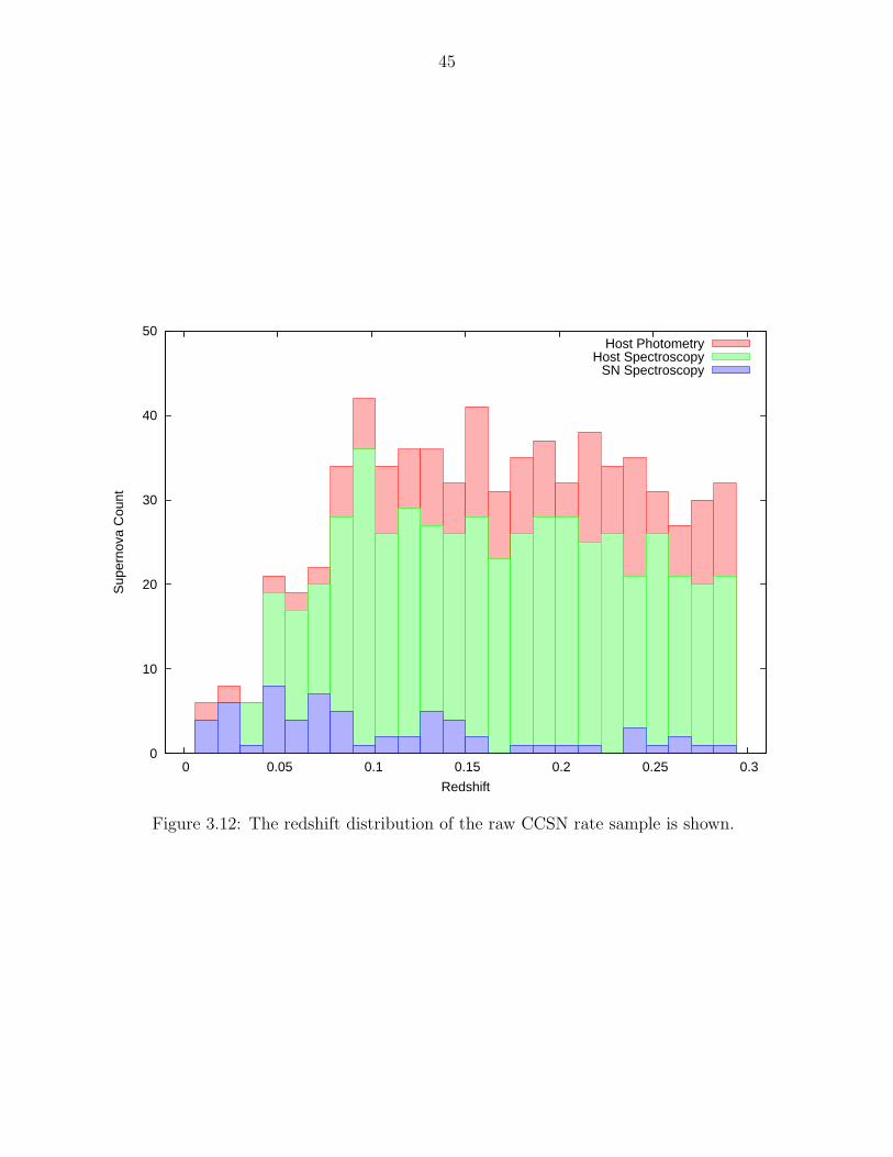
45
0
10
20
30
40
50
0 0.05 0.1 0.15 0.2 0.25 0.3
Sup
erno
va C
ount
Redshift
Host PhotometryHost Spectroscopy
SN Spectroscopy
Figure 3.12: The redshift distribution of the raw CCSN rate sample is shown.
46
dimmer, in the SDSS r band. As all other supernova rate measurements to date suffer the
same limitation, either implicitly or via an explicit luminosity requirement, my result will
still be comparable to other rate measurements in the literature.
For purposes of this rate measurement, I am interested in the comoving volume that
encloses the sample of supernovae. Comoving volume is defined as the space-time containing
a set of objects, projected onto a constant time surface that contains the present era on
Earth. In the redshift range of interest, the comoving distance as a function of redshift is
well approximated by:
DC(z) =
∫ z
0
DH(Ωm(1 + ζ)3 + ΩΛ)−1/2 dζ (3.10)
where DH = 4282.74Mpc is the Hubble distance. The parameters Ωm = 0.27 and ΩΛ =
0.73 represent the current consensus ΛCDM cosmology. [36] To convert comoving distance
to survey volume, I apply the following formula:
VC =1
3Ω(DC(z = 0.09)3 −DC(z = 0.03)3) (3.11)
where Ω is the solid angle surveyed in steradians.
Uncertainty in cosmological parameters could make a small contribution to uncertainty
in the comoving volume, and hence uncertainty in the supernova rate. However, this effect
is very small at the redshift range where we observe CCSN. To probe the effect of varying
cosmological parameters on comoving volume, I employed the iCosmos cosmological distance
calculator, developed by M. Vardanyan [37].
The SDSS-II SN cosmology study found roughly 5 percent uncertainty in Ωm [21], which
translates to approximately 0.3 percent uncertainty in comoving volume at z = 0.1. This
error due to uncertainty in Ωm, the cosmic matter density parameter, is an order of magnitude
smaller than other sources of error, and therefore I ignore it in this work.
Kessler et al. also found approximately 10 percent uncertainty in w [21], the dark energy
47
equation of state parameter, which translates to about 1.3 percent uncertainty in comoving
volume at z = 0.09. The effect of uncertainty in w is small, but it is significant enough
to account for in sources of error for the CCSN rate, and I have included it in the error
tabulation in Chapter four.
3.5 Supernova Time and Luminosity
A supernova rate measurement treats each supernova as an instantaneous event. This
view is physically appropriate, since a star’s initial core collapse event spans only a few
seconds of time. However, surveys such as SDSS-II have much coarser time resolution. Each
object is imaged at most once every two days, and the optically bright explosion evolves
much more slowly than the initial core collapse, on the scale of weeks or even months.
As is common in supernova research, I use the supernova’s peak luminosity in the SDSS
r band to mark its occurrence in time. While the time delay between initial core collapse
and peak luminosity can vary among supernovae, there is always exactly one peak per core
collapse. Therefore, the rate of observed luminosity peaks must equal the rate of core collapse
events.
I determine the peak luminosity and time of each light curve from its fitted model func-
tion. To exclude spurious peaks, I require that the peak occur at least 10 days after the
start of an SDSS-II viewing season, and at least 10 days prior to the end of a season. Also,
there must be at least one observation of the supernova preceding the peak by 12 hours or
more, and one following the peak by 12 hours or more. The 12 hour gap ensures that the
observation is not on the same night as the peak.
Because the SDSS-II viewing season is shorter than the observable duration of a super-
nova, there is a possibility that I could mistake a local maximum in the light curve for a
true luminosity peak. To estimate error due to this effect, I repeated the rate calculation
excluding an additional 10 days of each viewing season. In this test, the peak finding algo-
48
rithm only identified one false peak out of few hundred candidate light curves. Therefore, I
conclude that overcounting due to false peaks is not significant compared to other sources
of error.
3.6 Supernova Detection Efficiency Model
The magnitude limit, beyond which a supernova is too dim for the survey to detect, is
not a sharp boundary. There is a range of magnitudes in which supernovae have a finite
probability of detection, referred to as the survey’s detection efficiency. For this work, I
model the detection efficiency as a function of the supernova’s peak apparent magnitude, as
seen from Earth in the SDSS r band. The form of the model efficiency function, ε(m) is:
ε(m) =1
2(1 + cos(
π
σE
(m−mE))) (3.12)
in the range (mE < m < mE + σE), where m is the supernova peak magnitude.
Outside the range where ε(m) is defined, the efficiency is one (m < mE) or zero (m >
mE + σE). The first parameter, mE, defines the dimmest magnitude at which the survey’s
detection efficiency is perfect, for practical purposes. The second parameter, σE, defines the
width of the magnitude range over which the efficiency falls from unity to zero.
The model parameters, mE and σE, are chosen through a fitting routine. First, I build a
model for the supernova rate sample as a function of limiting magnitude, using only those
candidates bright enough that detection efficiency is nearly one. The number of candidates,
Np(m) is expected to have the form:
Np(m) = (p0 + p1100.6m + p2100.8m + p3101.0m + p4101.2m) (3.13)
where m is the limiting peak apparent magnitude in the SDSS r band.
Equation 3.13 may be derived by first expressing the SN rate, ρSN , as a function of
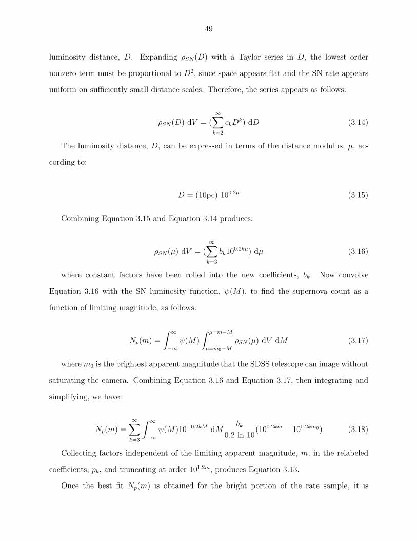
49
luminosity distance, D. Expanding ρSN(D) with a Taylor series in D, the lowest order
nonzero term must be proportional to D2, since space appears flat and the SN rate appears
uniform on sufficiently small distance scales. Therefore, the series appears as follows:
ρSN(D) dV = (∞∑
k=2
ckDk) dD (3.14)
The luminosity distance, D, can be expressed in terms of the distance modulus, µ, ac-
cording to:
D = (10pc) 100.2µ (3.15)
Combining Equation 3.15 and Equation 3.14 produces:
ρSN(µ) dV = (∞∑
k=3
bk100.2kµ) dµ (3.16)
where constant factors have been rolled into the new coefficients, bk. Now convolve
Equation 3.16 with the SN luminosity function, ψ(M), to find the supernova count as a
function of limiting magnitude, as follows:
Np(m) =
∫ ∞
−∞ψ(M)
∫ µ=m−M
µ=m0−M
ρSN(µ) dV dM (3.17)
where m0 is the brightest apparent magnitude that the SDSS telescope can image without
saturating the camera. Combining Equation 3.16 and Equation 3.17, then integrating and
simplifying, we have:
Np(m) =∞∑
k=3
∫ ∞
−∞ψ(M)10−0.2kM dM
bk0.2 ln 10
(100.2km − 100.2km0) (3.18)
Collecting factors independent of the limiting apparent magnitude, m, in the relabeled
coefficients, pk, and truncating at order 101.2m, produces Equation 3.13.
Once the best fit Np(m) is obtained for the bright portion of the rate sample, it is
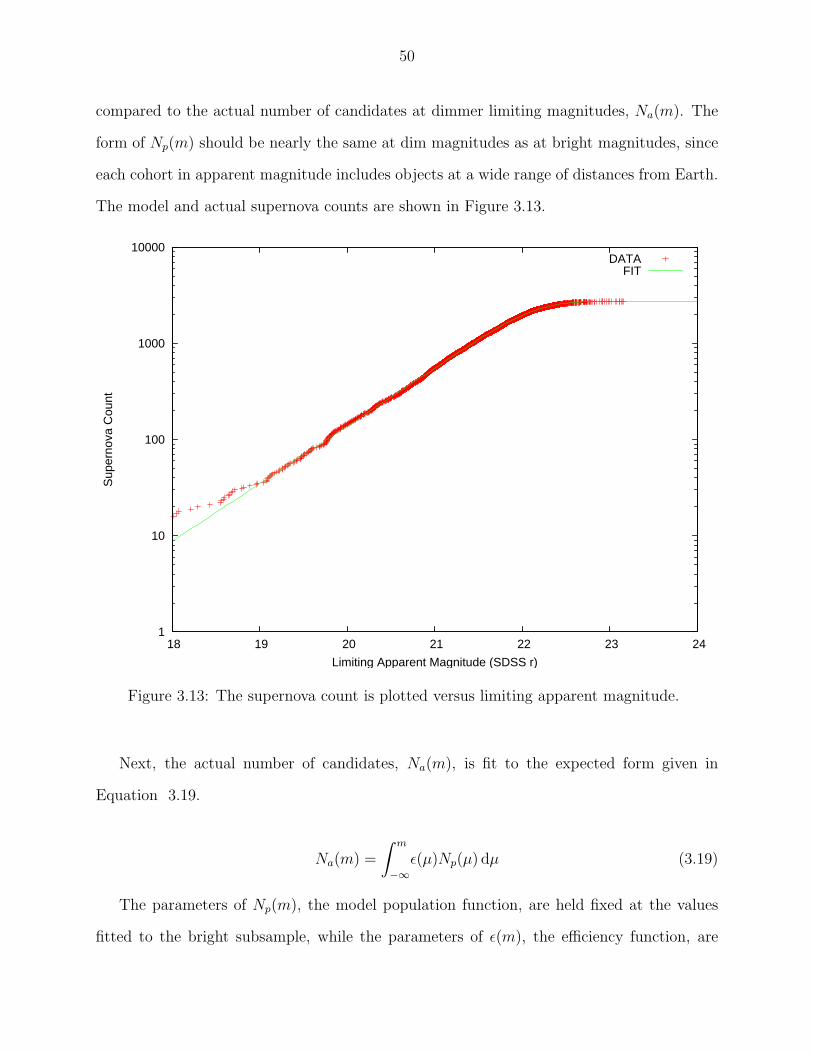
50
compared to the actual number of candidates at dimmer limiting magnitudes, Na(m). The
form of Np(m) should be nearly the same at dim magnitudes as at bright magnitudes, since
each cohort in apparent magnitude includes objects at a wide range of distances from Earth.
The model and actual supernova counts are shown in Figure 3.13.
1
10
100
1000
10000
18 19 20 21 22 23 24
Sup
erno
va C
ount
Limiting Apparent Magnitude (SDSS r)
DATAFIT
Figure 3.13: The supernova count is plotted versus limiting apparent magnitude.
Next, the actual number of candidates, Na(m), is fit to the expected form given in
Equation 3.19.
Na(m) =
∫ m
−∞ε(µ)Np(µ) dµ (3.19)
The parameters of Np(m), the model population function, are held fixed at the values
fitted to the bright subsample, while the parameters of ε(m), the efficiency function, are
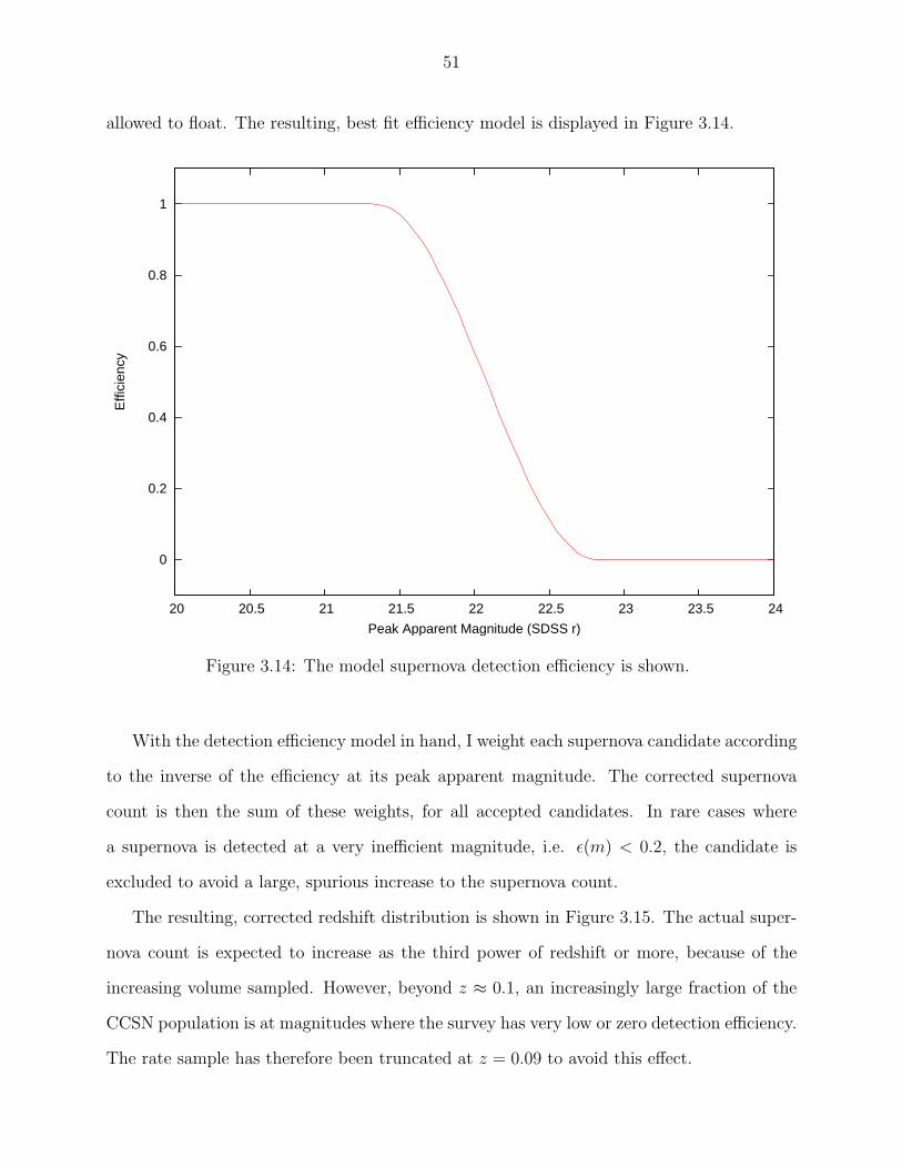
51
allowed to float. The resulting, best fit efficiency model is displayed in Figure 3.14.
0
0.2
0.4
0.6
0.8
1
20 20.5 21 21.5 22 22.5 23 23.5 24
Effi
cien
cy
Peak Apparent Magnitude (SDSS r)
Figure 3.14: The model supernova detection efficiency is shown.
With the detection efficiency model in hand, I weight each supernova candidate according
to the inverse of the efficiency at its peak apparent magnitude. The corrected supernova
count is then the sum of these weights, for all accepted candidates. In rare cases where
a supernova is detected at a very inefficient magnitude, i.e. ε(m) < 0.2, the candidate is
excluded to avoid a large, spurious increase to the supernova count.
The resulting, corrected redshift distribution is shown in Figure 3.15. The actual super-
nova count is expected to increase as the third power of redshift or more, because of the
increasing volume sampled. However, beyond z ≈ 0.1, an increasingly large fraction of the
CCSN population is at magnitudes where the survey has very low or zero detection efficiency.
The rate sample has therefore been truncated at z = 0.09 to avoid this effect.
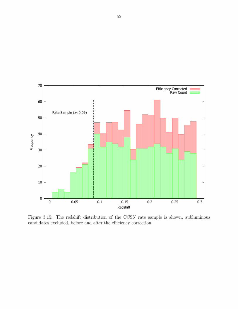
52
0
10
20
30
40
50
60
70
0 0.05 0.1 0.15 0.2 0.25 0.3
Fre
quency
Redshift
Efficiency CorrectedRaw Count
Rate Sample (z<0.09)
Figure 3.15: The redshift distribution of the CCSN rate sample is shown, subluminouscandidates excluded, before and after the efficiency correction.
53
3.7 Host Galaxy Extinction Model
The observed luminosity of a supernova may be less than its actual luminosity, a phe-
nomenon referred to as extinction. Extinction occurs due to the presence of dust, i.e. par-
ticles that scatter and/or absorb light, between the supernova and Earth. Dust within the
Milky Way is relatively well understood, and SDSS-II supernova light curves have already
been corrected for its effects by the SDSS-II Supernova Survey data pipeline. [21]
However, dust in each supernova’s host galaxy, or perhaps even in the local environment
of the supernova itself, is more difficult to measure. This local extinction is well represented
by the model of Cardelli et al. [38], which quantifies extinction of a bright source with two
parameters, AV and RV . The AV parameter specifies the change in magnitude due to dust
absorption, in the Johnson V band, and the RV parameter specifies the wavelength depen-
dence of dust absorption. Dust absorption is more pronounced at longer (red) wavelengths.
The central wavelength of the SDSS r filter, at 623 nm, lies between the Johnson R and
V filters, at 658 nm and 551 nm respectively. Cardelli et al. find that AR/AV ≈ 0.75 for the
standard value of RV = 3.1 in the diffuse interstellar medium [38]. Interpolating between
AR and AV to estimate extinction in the SDSS r band, I find that Ar/AV = 0.83.
Correcting for the effect of extinction on the observed supernova rate then requires a
statistical distribution of Ar for core collapse supernovae. I employ the model developed by
Hatano et al. [39], who simulated an ensemble of host galaxies at random inclinations, and
placed model supernovae within them approximating the spatial distribution of observed
supernovae. Dust along the resulting line of sight determined the extinction of each model
supernova. The resulting AV distribution is roughly exponential with exponent τ = 0.50±
0.03. Converting to SDSS r band scales τ in proportion to Ar/AV , yielding a corrected
exponent of τ = 0.42± 0.03.
P(Ar) ≈1
τe−
Arτ (3.20)
54
The number of observed supernova, Nobs(M), as a function of limiting magnitude, M , is
then given by:
Nobs(M) =
∫ ∞
−∞
dN
dm
∫ ∞
0
1
τe−
Arτ θ(M − (m+ Ar)) dAr dm (3.21)
The integral over Ar can be solved exactly, as follows:
Nobs(M) =
∫ ∞
−∞
dN
dm(1− e
m−Mτ ) dm = Nactual −
∫ ∞
−∞
dN
dme
m−Mτ dm (3.22)
Now take the derivative on both sides with respect to the limiting magnitude, M , and
simplify, resulting in the following:
Ncorrected(M)−Nobs(M) = τdNobs
dM(3.23)
The above is just the correction to the supernova count, due to extinction. To estimate
that correction, I fit a line to Nobs(M) in the vicinity of absolute magnitude -15.0, and take
the line’s slope as the value of dNobs/dM . Because of poorly quantified uncertainties in the
extinction model, I count 100% of this correction as a source of systematic error. Fortunately,
the extinction correction is small, less than 3 percent of the measured rate.
55
Chapter 4
Results
4.1 Supernova Count
The SDSS-II Supernova Survey had three viewing seasons of approximately 90 days each
from 2005-2007, in the Northern Hemisphere autumn when the Sun is located furthest from
the Stripe 82 region in Earth’s sky. Over these three seasons, the survey identified a total
of 10,606 supernova candidates which met the candidate criteria set forth by Frieman et
al. [20]:
• The automated object detection algorithm detects a change in brightness versus the
template, in two or more passbands.
• The object location is not on the veto list of known variable stars and galaxies.
• Human and software scans did not reject it as an artifact or Solar System object.
• The object was not active in multiple viewing seasons.
Of these, 9,934 candidates were active within the time and space constraints I chose for the
core collapse rate sample, i.e. between right ascension −50 to +55, and in the 2005, 2006
or 2007 viewing season.
56
Phenomenological light curve fitting, using the method of Bazin et al. [1], rejected 50
candidates with null or negative flux in all epochs, and another 12 candidates for which the
fit did not converge. The latter 12 light curves are displayed in Figures 3.5- 3.6.
After fitting light curves to the Bazin model, I excluded all candidates where the model
peak occurs in the first or last 10 days of a viewing season, or where there is not at least one
observation 12 hours prior and 12 hours following the peak. This requirement removed 479
candidates. The peak time distribution of the remaining sample is displayed in Figure 4.1.
While the raw distribution shows systematic time bias, filtering by peak magnitude shows
that the bias primarily affects objects dimmer than peak magnitude 22.0, near the limit of
the survey depth.
The quality of the light curve fit is measured using the flatness score, Λ, defined in
Equation 3.7, as explained in Ch. 3.3. I removed a total of 6,513 candidates from the
rate sample for exceeding the flatness score threshold, Λc = 0.354, nearly 70 percent of
candidates. However, the great majority of such candidates are well beyond Λc, in a range
where confirmed supernovae occur very rarely, as shown in Figure 3.7.
To locate a supernova candidate in three dimensional space, I require a distance measure-
ment, in addition to its angular coordinates. I use cosmic redshift as a distance indicator,
according to the formula for comoving distance as a function of redshift described in Ch. 3.4.
Spectroscopic redshift of the supernova itself is preferred, but when that is not available I
instead use the spectroscopic redshift of the host galaxy, or a photometric redshift estimate
of the host galaxy as a last resort. However, in a few cases no spectra were taken of the
supernova, and the host galaxy is too faint to detect, thus I have no guidance at all for the
candidate’s distance.
I removed 150 candidates from the sample due to lack of redshift information, treating
all of them as non-detections. Figure 4.2 shows the peak magnitude distribution of such
candidates. By treating candidates with no redshift as non-detections, I aim to correct for
their omission with the detection efficiency model, especially since redshift is most likely
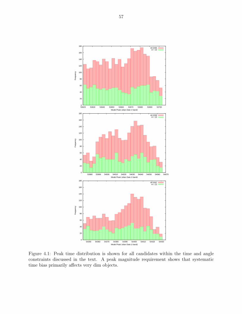
57
0
20
40
60
80
100
120
140
160
180
53620 53630 53640 53650 53660 53670 53680 53690 53700
Fre
quen
cy
Model Peak Julian Date (r band)
All 2005m < 22
0
20
40
60
80
100
120
140
160
180
53980 53990 54000 54010 54020 54030 54040 54050 54060 54070
Fre
quen
cy
Model Peak Julian Date (r band)
All 2006m < 22
0
20
40
60
80
100
120
140
160
180
54350 54360 54370 54380 54390 54400 54410 54420 54430
Fre
quen
cy
Model Peak Julian Date (r band)
All 2007m < 22
Figure 4.1: Peak time distribution is shown for all candidates within the time and angleconstraints discussed in the text. A peak magnitude requirement shows that systematictime bias primarily affects very dim objects.
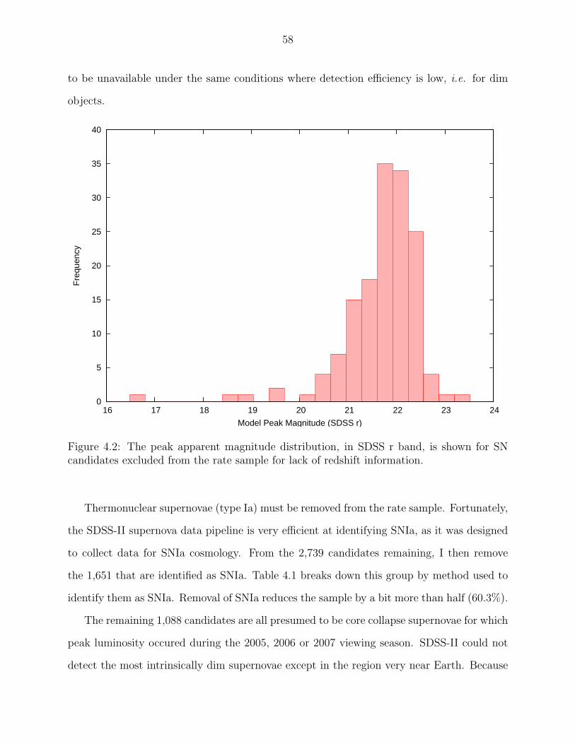
58
to be unavailable under the same conditions where detection efficiency is low, i.e. for dim
objects.
0
5
10
15
20
25
30
35
40
16 17 18 19 20 21 22 23 24
Fre
quen
cy
Model Peak Magnitude (SDSS r)
Figure 4.2: The peak apparent magnitude distribution, in SDSS r band, is shown for SNcandidates excluded from the rate sample for lack of redshift information.
Thermonuclear supernovae (type Ia) must be removed from the rate sample. Fortunately,
the SDSS-II supernova data pipeline is very efficient at identifying SNIa, as it was designed
to collect data for SNIa cosmology. From the 2,739 candidates remaining, I then remove
the 1,651 that are identified as SNIa. Table 4.1 breaks down this group by method used to
identify them as SNIa. Removal of SNIa reduces the sample by a bit more than half (60.3%).
The remaining 1,088 candidates are all presumed to be core collapse supernovae for which
peak luminosity occured during the 2005, 2006 or 2007 viewing season. SDSS-II could not
detect the most intrinsically dim supernovae except in the region very near Earth. Because
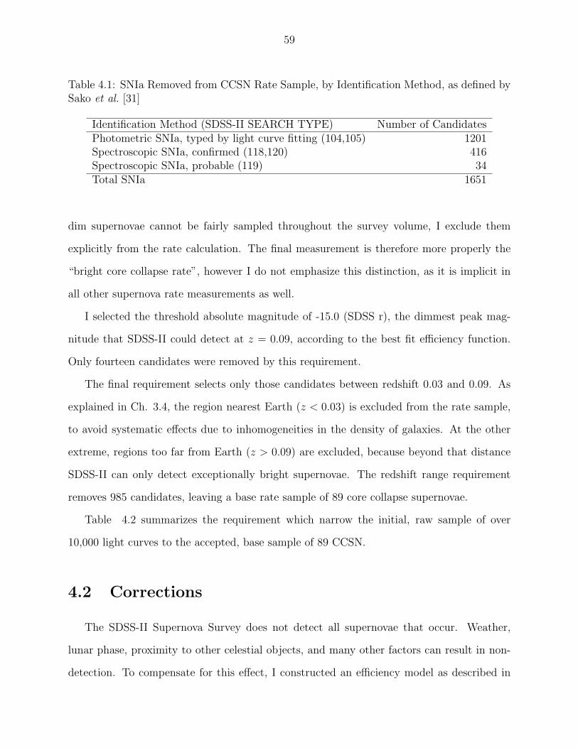
59
Table 4.1: SNIa Removed from CCSN Rate Sample, by Identification Method, as defined bySako et al. [31]
Identification Method (SDSS-II SEARCH TYPE) Number of CandidatesPhotometric SNIa, typed by light curve fitting (104,105) 1201Spectroscopic SNIa, confirmed (118,120) 416Spectroscopic SNIa, probable (119) 34Total SNIa 1651
dim supernovae cannot be fairly sampled throughout the survey volume, I exclude them
explicitly from the rate calculation. The final measurement is therefore more properly the
“bright core collapse rate”, however I do not emphasize this distinction, as it is implicit in
all other supernova rate measurements as well.
I selected the threshold absolute magnitude of -15.0 (SDSS r), the dimmest peak mag-
nitude that SDSS-II could detect at z = 0.09, according to the best fit efficiency function.
Only fourteen candidates were removed by this requirement.
The final requirement selects only those candidates between redshift 0.03 and 0.09. As
explained in Ch. 3.4, the region nearest Earth (z < 0.03) is excluded from the rate sample,
to avoid systematic effects due to inhomogeneities in the density of galaxies. At the other
extreme, regions too far from Earth (z > 0.09) are excluded, because beyond that distance
SDSS-II can only detect exceptionally bright supernovae. The redshift range requirement
removes 985 candidates, leaving a base rate sample of 89 core collapse supernovae.
Table 4.2 summarizes the requirement which narrow the initial, raw sample of over
10,000 light curves to the accepted, base sample of 89 CCSN.
4.2 Corrections
The SDSS-II Supernova Survey does not detect all supernovae that occur. Weather,
lunar phase, proximity to other celestial objects, and many other factors can result in non-
detection. To compensate for this effect, I constructed an efficiency model as described in
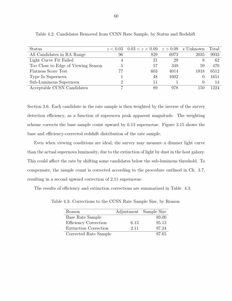
60
Table 4.2: Candidates Removed from CCSN Rate Sample, by Status and Redshift
Status z < 0.03 0.03 < z < 0.09 z > 0.09 z Unknown TotalAll Candidates in RA Range 96 829 6973 2035 9933Light Curve Fit Failed 4 21 29 8 62Too Close to Edge of Viewing Season 5 57 349 59 470Flatness Score Test 77 603 4014 1818 6512Type Ia Supernova 1 48 1602 0 1651Sub-Luminous Supernova 2 11 1 0 14Acceptable CCSN Candidates 7 89 978 150 1224
Section 3.6. Each candidate in the rate sample is then weighted by the inverse of the survey
detection efficiency, as a function of supernova peak apparent magnitude. The weighting
scheme corrects the base sample count upward by 6.13 supernovae. Figure 3.15 shows the
base and efficiency-corrected redshift distribution of the rate sample.
Even when viewing conditions are ideal, the survey may measure a dimmer light curve
than the actual supernova luminosity, due to the extinction of light by dust in the host galaxy.
This could affect the rate by shifting some candidates below the sub-luminous threshold. To
compensate, the sample count is corrected according to the procedure outlined in Ch. 3.7,
resulting in a second upward correction of 2.11 supernovae.
The results of efficiency and extinction corrections are summarized in Table 4.3.
Table 4.3: Corrections to the CCSN Rate Sample Size, by Reason
Reason Adjustment Sample SizeBase Rate Sample 89.00Efficiency Correction 6.13 95.13Extinction Correction 2.11 97.24Corrected Rate Sample 97.65
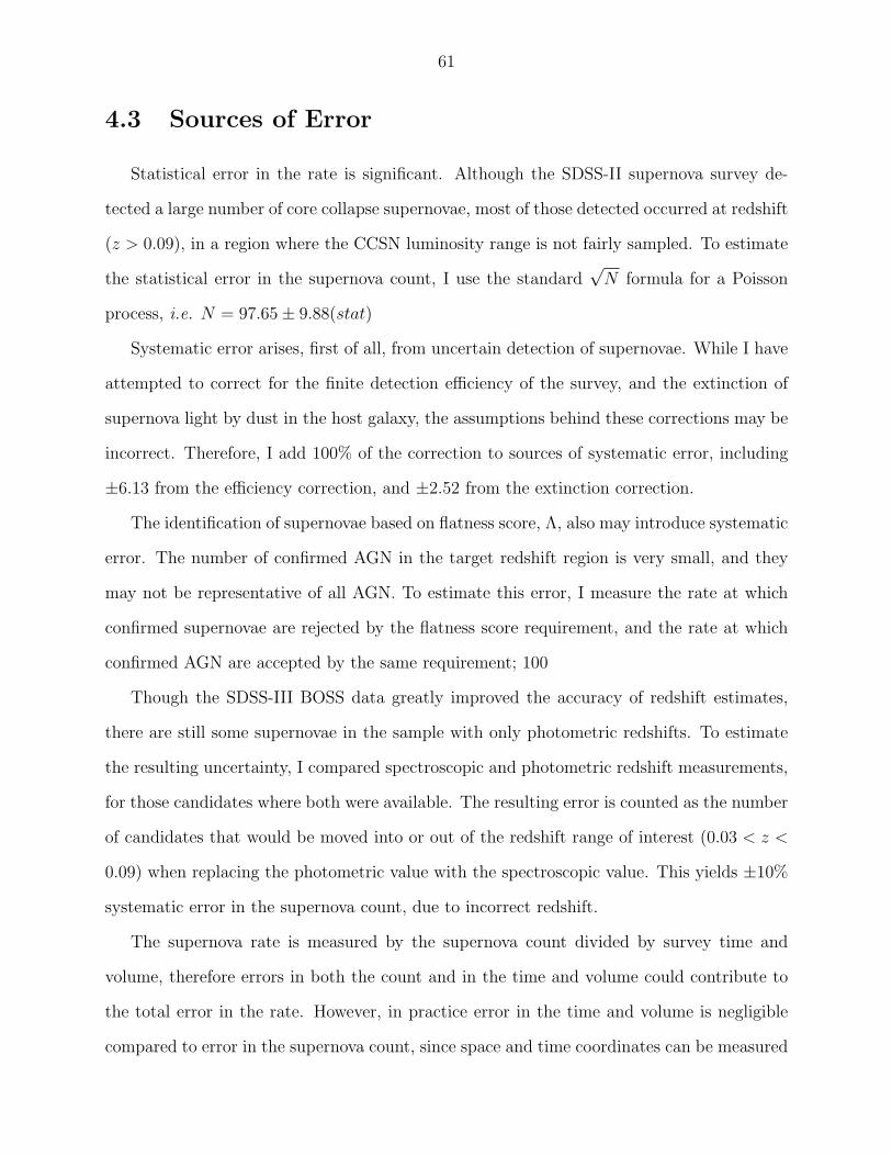
61
4.3 Sources of Error
Statistical error in the rate is significant. Although the SDSS-II supernova survey de-
tected a large number of core collapse supernovae, most of those detected occurred at redshift
(z > 0.09), in a region where the CCSN luminosity range is not fairly sampled. To estimate
the statistical error in the supernova count, I use the standard√N formula for a Poisson
process, i.e. N = 97.65± 9.88(stat)
Systematic error arises, first of all, from uncertain detection of supernovae. While I have
attempted to correct for the finite detection efficiency of the survey, and the extinction of
supernova light by dust in the host galaxy, the assumptions behind these corrections may be
incorrect. Therefore, I add 100% of the correction to sources of systematic error, including
±6.13 from the efficiency correction, and ±2.52 from the extinction correction.
The identification of supernovae based on flatness score, Λ, also may introduce systematic
error. The number of confirmed AGN in the target redshift region is very small, and they
may not be representative of all AGN. To estimate this error, I measure the rate at which
confirmed supernovae are rejected by the flatness score requirement, and the rate at which
confirmed AGN are accepted by the same requirement; 100
Though the SDSS-III BOSS data greatly improved the accuracy of redshift estimates,
there are still some supernovae in the sample with only photometric redshifts. To estimate
the resulting uncertainty, I compared spectroscopic and photometric redshift measurements,
for those candidates where both were available. The resulting error is counted as the number
of candidates that would be moved into or out of the redshift range of interest (0.03 < z <
0.09) when replacing the photometric value with the spectroscopic value. This yields ±10%
systematic error in the supernova count, due to incorrect redshift.
The supernova rate is measured by the supernova count divided by survey time and
volume, therefore errors in both the count and in the time and volume could contribute to
the total error in the rate. However, in practice error in the time and volume is negligible
compared to error in the supernova count, since space and time coordinates can be measured
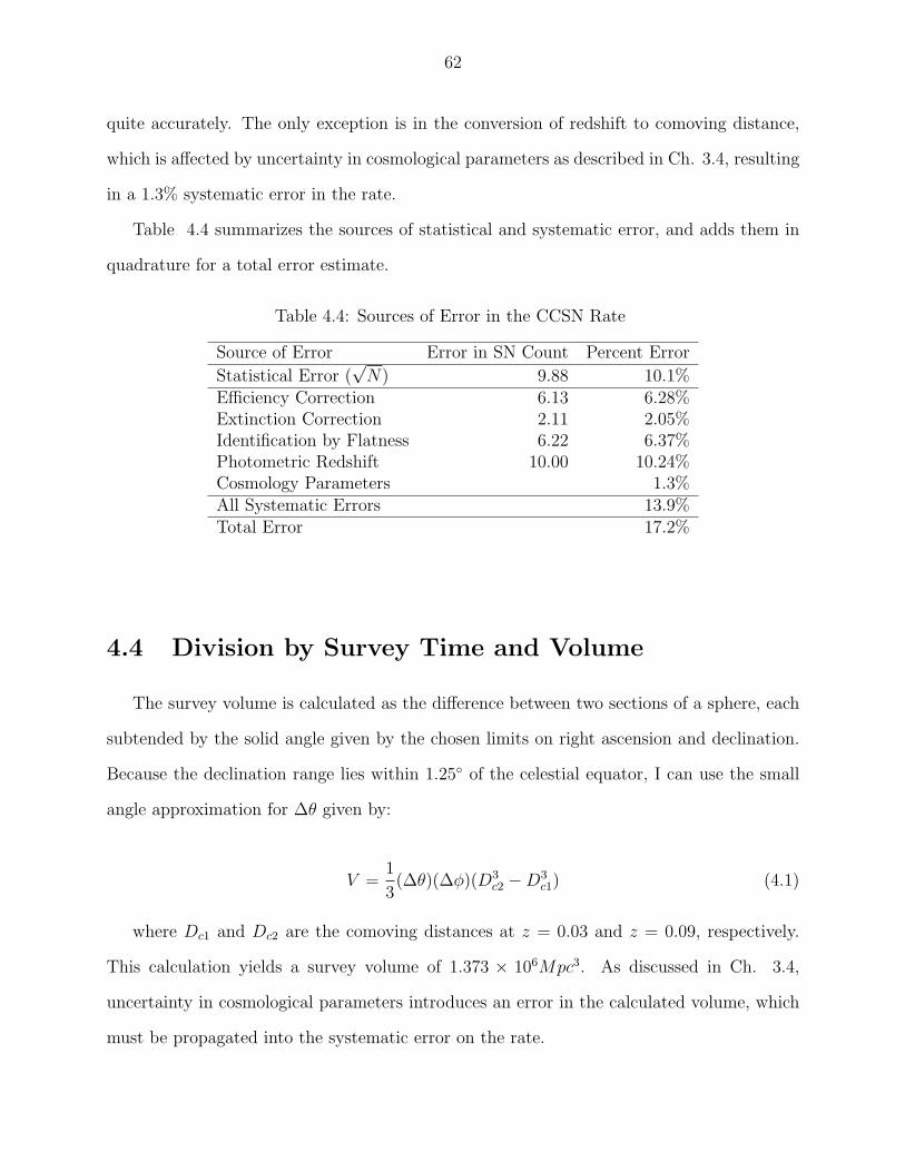
62
quite accurately. The only exception is in the conversion of redshift to comoving distance,
which is affected by uncertainty in cosmological parameters as described in Ch. 3.4, resulting
in a 1.3% systematic error in the rate.
Table 4.4 summarizes the sources of statistical and systematic error, and adds them in
quadrature for a total error estimate.
Table 4.4: Sources of Error in the CCSN Rate
Source of Error Error in SN Count Percent Error
Statistical Error (√N) 9.88 10.1%
Efficiency Correction 6.13 6.28%Extinction Correction 2.11 2.05%Identification by Flatness 6.22 6.37%Photometric Redshift 10.00 10.24%Cosmology Parameters 1.3%All Systematic Errors 13.9%Total Error 17.2%
4.4 Division by Survey Time and Volume
The survey volume is calculated as the difference between two sections of a sphere, each
subtended by the solid angle given by the chosen limits on right ascension and declination.
Because the declination range lies within 1.25 of the celestial equator, I can use the small
angle approximation for ∆θ given by:
V =1
3(∆θ)(∆φ)(D3
c2 −D3c1) (4.1)
where Dc1 and Dc2 are the comoving distances at z = 0.03 and z = 0.09, respectively.
This calculation yields a survey volume of 1.373 × 10⁶Mpc3. As discussed in Ch. 3.4,
uncertainty in cosmological parameters introduces an error in the calculated volume, which
must be propagated into the systematic error on the rate.
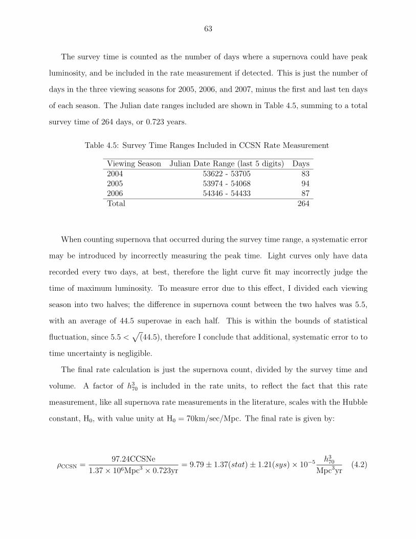
63
The survey time is counted as the number of days where a supernova could have peak
luminosity, and be included in the rate measurement if detected. This is just the number of
days in the three viewing seasons for 2005, 2006, and 2007, minus the first and last ten days
of each season. The Julian date ranges included are shown in Table 4.5, summing to a total
survey time of 264 days, or 0.723 years.
Table 4.5: Survey Time Ranges Included in CCSN Rate Measurement
Viewing Season Julian Date Range (last 5 digits) Days2004 53622 - 53705 832005 53974 - 54068 942006 54346 - 54433 87Total 264
When counting supernova that occurred during the survey time range, a systematic error
may be introduced by incorrectly measuring the peak time. Light curves only have data
recorded every two days, at best, therefore the light curve fit may incorrectly judge the
time of maximum luminosity. To measure error due to this effect, I divided each viewing
season into two halves; the difference in supernova count between the two halves was 5.5,
with an average of 44.5 superovae in each half. This is within the bounds of statistical
fluctuation, since 5.5 <√
(44.5), therefore I conclude that additional, systematic error to to
time uncertainty is negligible.
The final rate calculation is just the supernova count, divided by the survey time and
volume. A factor of h370 is included in the rate units, to reflect the fact that this rate
measurement, like all supernova rate measurements in the literature, scales with the Hubble
constant, H0, with value unity at H0 = 70km/sec/Mpc. The final rate is given by:
ρCCSN =97.24CCSNe
1.37× 10⁶Mpc3 × 0.723yr= 9.79± 1.37(stat)± 1.21(sys)× 10−5 h3
70
Mpc3yr(4.2)
64
Chapter 5
Conclusion
5.1 Comparison with Prior Measurements
To compare my core collapse rate result with other measurements in the literature, I
must first relate it to cosmic history. It is known that the star formation rate has evolved
throughout the history of the universe [40]. Because the rate at which massive stars are
created is time-dependent, the rate at which massive stars are destroyed must also be time-
dependent. Therefore, the core collapse supernova rate is not a universal constant, but a
function of time.
Any astronomical observation has an inherent time delay, due to the finite speed at which
light propagates from the source to Earth. In extragalactic astronomy, this lookback time is
very well correlated with an object’s cosmic redshift, according to the Hubble law. Because
my CCSN rate sample spans a range of redshifts, it also spans a range of cosmic history.
The number of CCSN in the sample, divided by time and volume, is an average over this
time range, not an instantaneous rate.
In order to compare my result to previous CCSN rate measurements, it is useful to
find the approximate redshift at which the average redshift over the entire bin is equal to
instantaneous CCSN rate. I refer to this matching redshift as zmatch. To determine zmatch, I
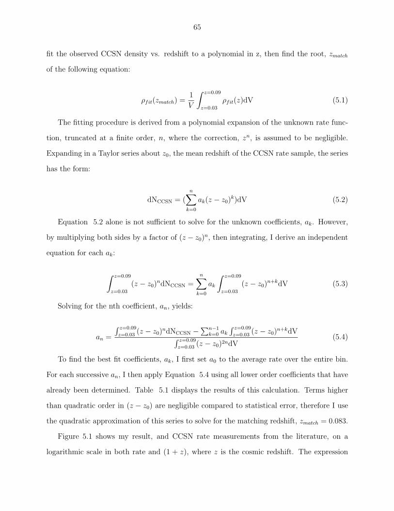
65
fit the observed CCSN density vs. redshift to a polynomial in z, then find the root, zmatch
of the following equation:
ρfit(zmatch) =1
V
∫ z=0.09
z=0.03
ρfit(z)dV (5.1)
The fitting procedure is derived from a polynomial expansion of the unknown rate func-
tion, truncated at a finite order, n, where the correction, zn, is assumed to be negligible.
Expanding in a Taylor series about z0, the mean redshift of the CCSN rate sample, the series
has the form:
dNCCSN = (n∑
k=0
ak(z − z0)k)dV (5.2)
Equation 5.2 alone is not sufficient to solve for the unknown coefficients, ak. However,
by multiplying both sides by a factor of (z − z0)n, then integrating, I derive an independent
equation for each ak:
∫ z=0.09
z=0.03
(z − z0)ndNCCSN =
n∑k=0
ak
∫ z=0.09
z=0.03
(z − z0)n+kdV (5.3)
Solving for the nth coefficient, an, yields:
an =
∫ z=0.09
z=0.03(z − z0)
ndNCCSN −∑n−1
k=0 ak
∫ z=0.09
z=0.03(z − z0)
n+kdV∫ z=0.09
z=0.03(z − z0)2ndV
(5.4)
To find the best fit coefficients, ak, I first set a0 to the average rate over the entire bin.
For each successive an, I then apply Equation 5.4 using all lower order coefficients that have
already been determined. Table 5.1 displays the results of this calculation. Terms higher
than quadratic order in (z − z0) are negligible compared to statistical error, therefore I use
the quadratic approximation of this series to solve for the matching redshift, zmatch = 0.083.
Figure 5.1 shows my result, and CCSN rate measurements from the literature, on a
logarithmic scale in both rate and (1 + z), where z is the cosmic redshift. The expression
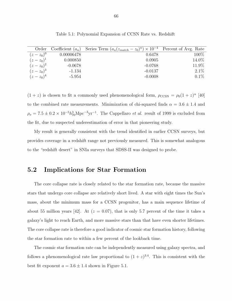
66
Table 5.1: Polynomial Expansion of CCSN Rate vs. Redshift
Order Coefficient (an) Series Term (an(zmatch − z0)n)× 10−4 Percent of Avg. Rate
(z − z0)0 0.00006478 0.6478 100%
(z − z0)1 0.000850 0.0905 14.0%
(z − z0)2 -0.0678 -0.0768 11.9%
(z − z0)3 -1.134 -0.0137 2.1%
(z − z0)4 -5.954 -0.0008 0.1%
(1 + z) is chosen to fit a commonly used phenomenological form, ρCCSN = ρ0(1 + z)α [40]
to the combined rate measurements. Minimization of chi-squared finds α = 3.6 ± 1.4 and
ρo = 7.5 ± 0.2 × 10⁻⁵h370Mpc−3yr−1. The Cappellaro et al. result of 1999 is excluded from
the fit, due to suspected underestimation of error in that pioneering study.
My result is generally consistent with the trend identified in earlier CCSN surveys, but
provides coverage in a redshift range not previously measured. This is somewhat analogous
to the “redshift desert” in SNIa surveys that SDSS-II was designed to probe.
5.2 Implications for Star Formation
The core collapse rate is closely related to the star formation rate, because the massive
stars that undergo core collapse are relatively short lived. A star with eight times the Sun’s
mass, about the minimum mass for a CCSN progenitor, has a main sequence lifetime of
about 55 million years [42]. At (z = 0.07), that is only 5.7 percent of the time it takes a
galaxy’s light to reach Earth, and more massive stars than that have even shorter lifetimes.
The core collapse rate is therefore a good indicator of cosmic star formation history, following
the star formation rate to within a few percent of the lookback time.
The cosmic star formation rate can be independently measured using galaxy spectra, and
follows a phenomenological rate law proportional to (1 + z)3.4. This is consistent with the
best fit exponent a = 3.6± 1.4 shown in Figure 5.1.
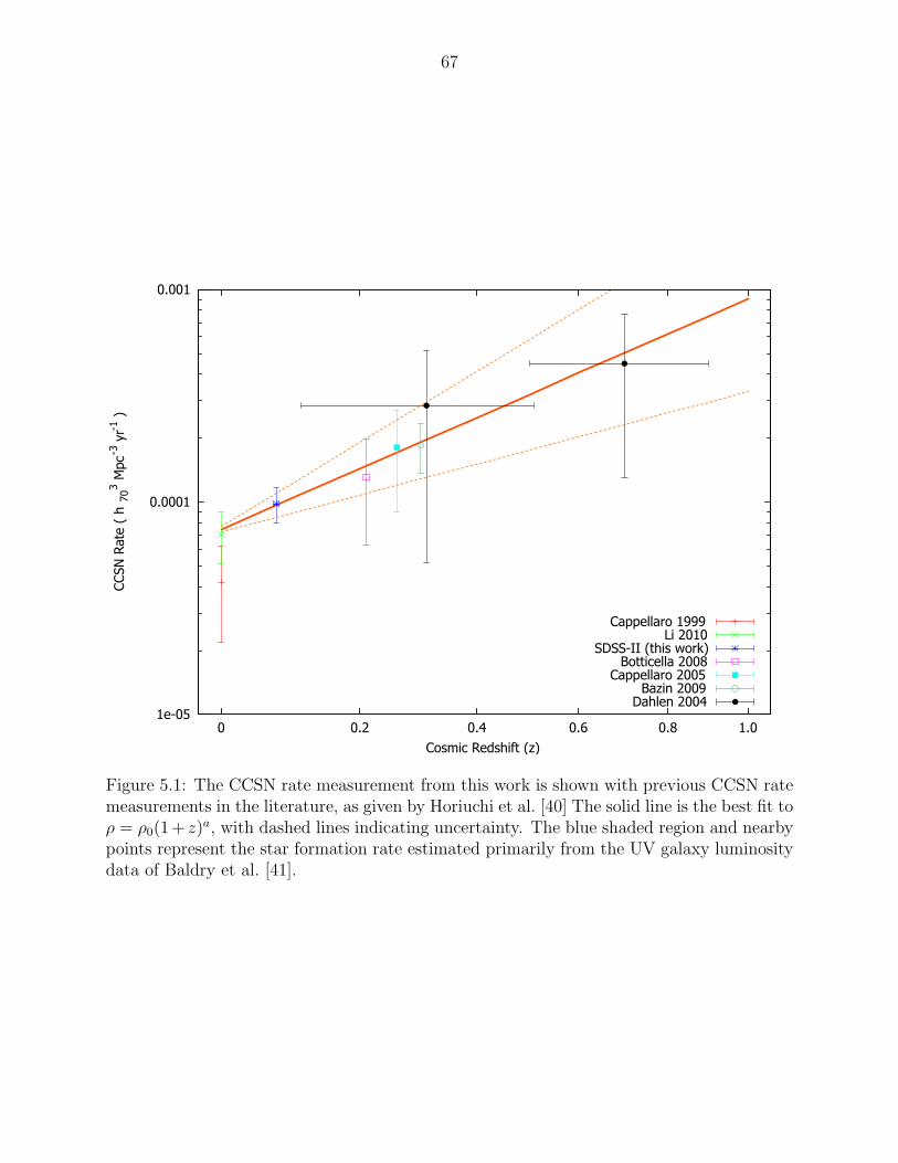
67
1e-05
0.0001
0.001
1.00.80.60.40.20
CCSN
Rate
( h
703 M
pc
-3 y
r-1 )
Cosmic Redshift (z)
Cappellaro 1999Li 2010
SDSS-II (this work)Botticella 2008
Cappellaro 2005Bazin 2009
Dahlen 2004
Figure 5.1: The CCSN rate measurement from this work is shown with previous CCSN ratemeasurements in the literature, as given by Horiuchi et al. [40] The solid line is the best fit toρ = ρ0(1+ z)a, with dashed lines indicating uncertainty. The blue shaded region and nearbypoints represent the star formation rate estimated primarily from the UV galaxy luminositydata of Baldry et al. [41].
68
As expected, the core collapse rate is proportional to the star formation rate. However,
the constant of proportionality is not consistent with stellar population models, as discovered
by Horiuchi it et al. [40]. They found that the observed CCSN rate falls short of the prediction
from the star formation rate by approximately a factor of two. Figure 5.2, taken from their
paper and updated to include the present work, shows this discrepancy.
Horiuchi et al. frame the disagreement between star formation and CCSN rates as a
“supernova rate problem”, a gap in our current understanding of stellar evolution. Either
we have only observed half of all CCSN that actually occur, our models of the stellar mass
distribution are flawed, or a portion of massive stars have a fate other than to explode as a
CCSN.
5.3 The CCSN Luminosity Function
With the SDSS-II supernova data, I can explore one aspect of the problem raised by Ho-
riuchi, the number of CCSN not observed because they are too dim. Horiuchi divides CCSN
into two categories, bright and faint. Bright CCSN are those with absolute V magnitude of
-15.0 or brighter. The V or visual band refers to the Johnson filter system, and is roughly
similar to the SDSS r band. An object’s absolute magnitude, M, is related to its redshift, z,
and apparent magnitude, m, as follows:
m = M + µ(z) (5.5)
The quantity, µ(z), is known as the distance modulus, a logarithmic measure of the
object’s distance. The formula for distance modulus as a function of redshift is:
µ(z) = 43.16 + 5log10(z2 + 2z
z2 + 2z + 2) (5.6)
Equation 5.6 makes a somewhat simplistic assumption of perfectly flat cosmology, in order
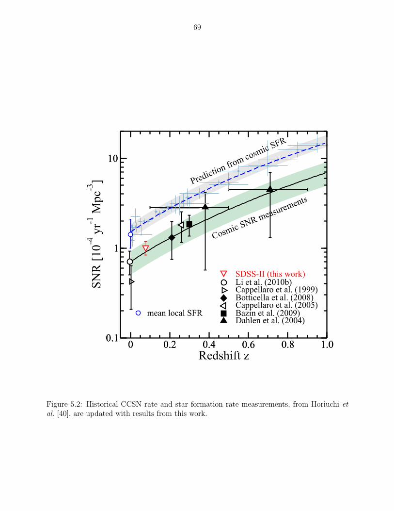
69
0 0.2 0.4 0.6 0.8 1.0Redshift z
0.1
1
10
SN
R [
10-4
yr-1
Mpc
-3]
Li et al. (2010b)Cappellaro et al. (1999)Botticella et al. (2008)Cappellaro et al. (2005)Bazin et al. (2009)Dahlen et al. (2004)
0 0.2 0.4 0.6 0.8 1.00.1
1
10
mean local SFR
Prediction from cosmic SFR
Cosmic SNR measurements
SDSS-II (this work)
Figure 5.2: Historical CCSN rate and star formation rate measurements, from Horiuchi etal. [40], are updated with results from this work.
70
to reduce the complexity of the calculation. However, it is within 0.24 magnitudes of the
value predicted by standard ΛCDM cosmology for a redshift of z = 0.09. Of the supernova
candidates in my core collapse rate sample, there are none which would be demoted to the
“subluminous” category by a shift of 0.24 magnitudes, and vice versa, therefore I conclude
that cosmological uncertainty in absolute magnitude affects the rate measurement negligibly,
compared to other sources of error.
Figure 5.3 shows the efficiency-weighted absolute magnitude distribution of my CCSN
rate sample, plus those candidates excluded only because of they were too faint or were
too near Earth. This distribution is also known as the core collapse supernova luminosity
function. Error on each bin count is estimated as√N assuming supernovae are a Poisson
process, added in quadrature with the 13.9 percent systematic error found for the supernova
count in Chapter 4.
In Figure 5.3, we see that subluminous supernovae are underrepresented in the full rate
sample, because they are only detected when relatively near Earth. To estimate the actual
rate of subluminous supernovae, I examine the subsamples for z < 0.06 and z < 0.03. The
subluminous fractions in these ranges are 20 percent and 24 percent respectively. Statistics
are too low to regard these figures as conclusive, but they do suggest that a subluminous
fraction of 50 percent, the number required to solve Horiuchi’s rate problem, is unlikely.
5.4 Potential for Future Measurements
Future astronomical survey instruments, such the Large Synoptic Survey Telescope (LSST)
[43], promise orders of magnitude increase in the number of supernovae observed, including
core collapse supernovae. While this will greatly reduce statistical error, systematic error
is likely to remain comparable to present day surveys, especially because only a fraction
of such events will have spectroscopic redshift measurements. Therefore, the CCSN rate
measurements themselves may not be much more accurate than today.

71
0
5
10
15
20
25
30
35
40
-20 -18 -16 -14 -12 -10
Fre
quency
Peak Absolute Magnitude (SDSS r)
z < 0.09z < 0.06z < 0.03
subluminous (M > -15)
Figure 5.3: A CCSN luminosity function is derived for the rate sample in this work, pluscandidates excluded only because they were faint or too near Earth.
72
On the other hand, greater statistics will be very important in better measuring the
rate of subluminous CCSN, a crucial factor in solving Horiuchi’s supernova rate problem.
Also, the increased statistics will be invaluable in more complex supernova measurements,
like understanding the distribution of various supernova characteristics within the CCSN
population, and correlating CCSN rate and characteristics with properties of the host galaxy,
and location within the galaxy.
In the meantime, the CCSN rate problem can be attacked from the other direction, by
investigating hypothetical modes of stellar death other than a CCSN explosion. For example,
a measurement of the local neutron star and black hole birth rates could show whether some
of the “missing” massive stars end their lives through direct formation of black holes, with no
accompanying bright explosion. Or perhaps, as Horiuchi speculates, the CCSN rate problem
will one day be solved by a major rethinking of stellar evolution and supernova physics.
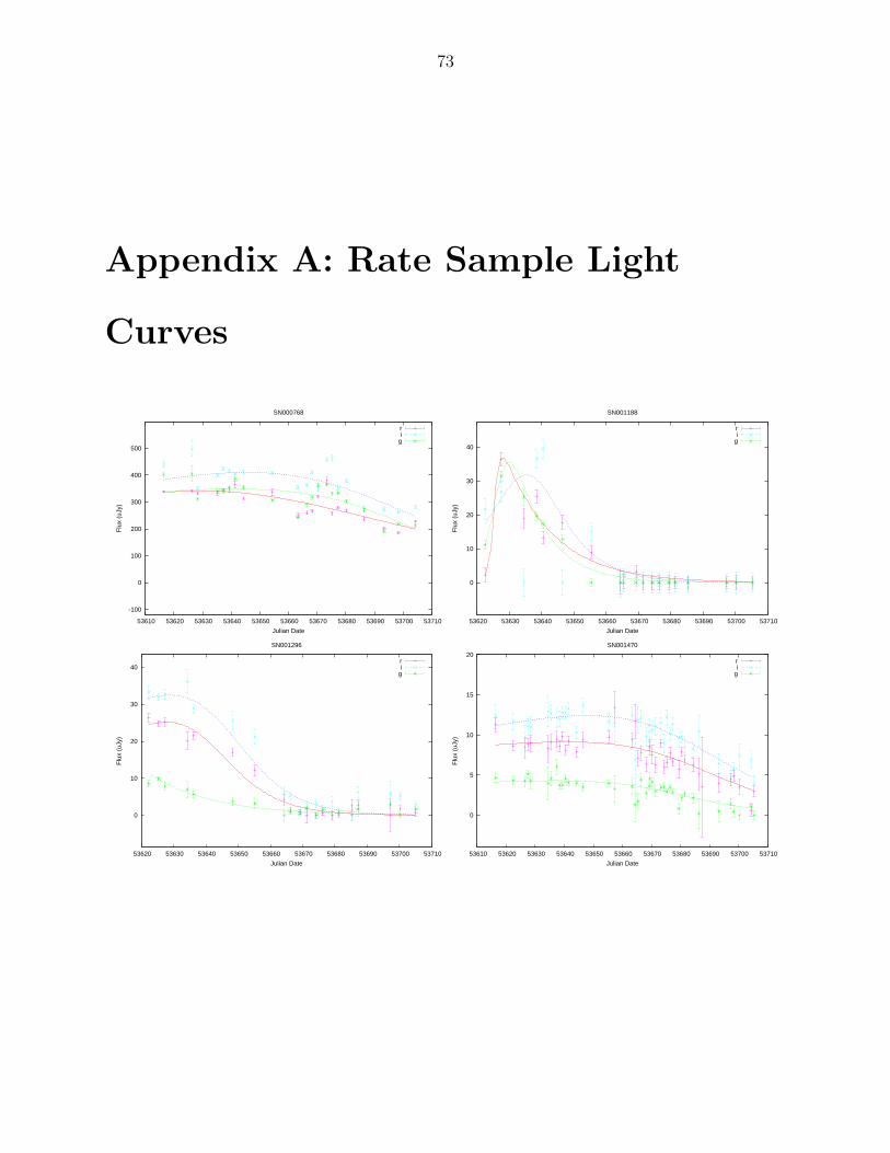
73
Appendix A: Rate Sample Light
Curves
-100
0
100
200
300
400
500
53610 53620 53630 53640 53650 53660 53670 53680 53690 53700 53710
Flu
x (u
Jy)
Julian Date
SN000768
ri
g
0
10
20
30
40
53620 53630 53640 53650 53660 53670 53680 53690 53700 53710
Flu
x (u
Jy)
Julian Date
SN001188
ri
g
0
10
20
30
40
53620 53630 53640 53650 53660 53670 53680 53690 53700 53710
Flu
x (u
Jy)
Julian Date
SN001296
ri
g
0
5
10
15
20
53610 53620 53630 53640 53650 53660 53670 53680 53690 53700 53710
Flu
x (u
Jy)
Julian Date
SN001470
ri
g
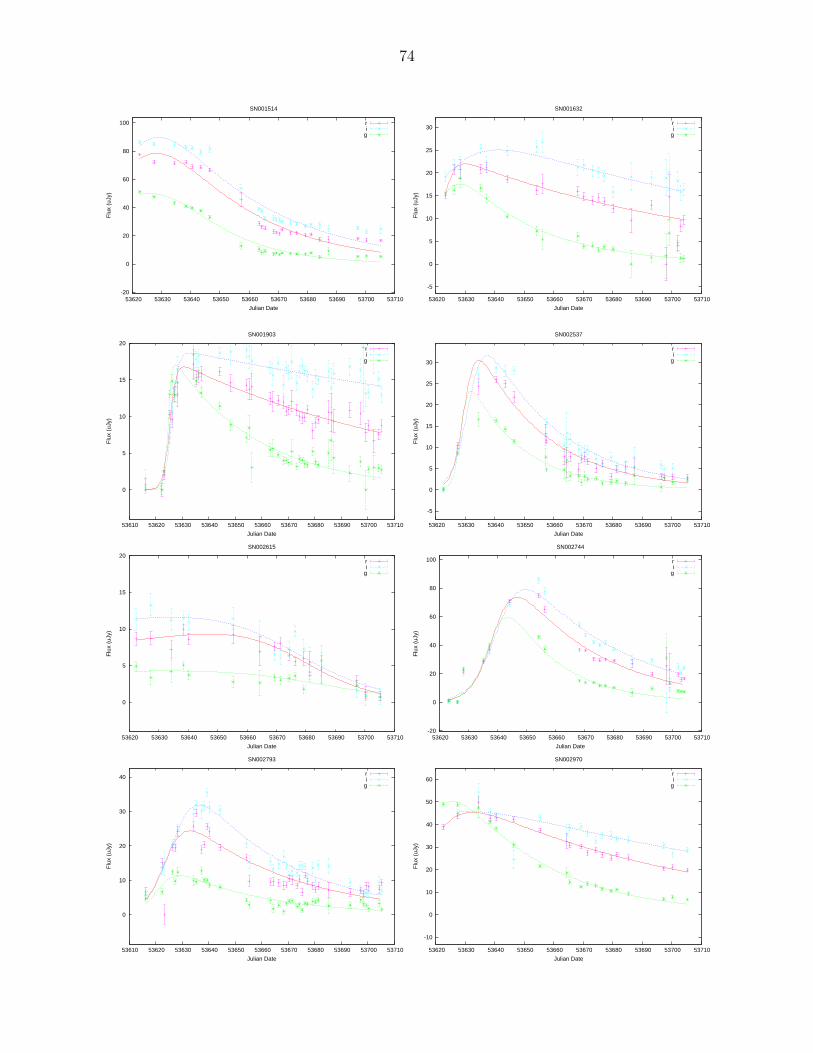
74
-20
0
20
40
60
80
100
53620 53630 53640 53650 53660 53670 53680 53690 53700 53710
Flu
x (u
Jy)
Julian Date
SN001514
ri
g
-5
0
5
10
15
20
25
30
53620 53630 53640 53650 53660 53670 53680 53690 53700 53710
Flu
x (u
Jy)
Julian Date
SN001632
ri
g
0
5
10
15
20
53610 53620 53630 53640 53650 53660 53670 53680 53690 53700 53710
Flu
x (u
Jy)
Julian Date
SN001903
ri
g
-5
0
5
10
15
20
25
30
53620 53630 53640 53650 53660 53670 53680 53690 53700 53710
Flu
x (u
Jy)
Julian Date
SN002537
ri
g
0
5
10
15
20
53620 53630 53640 53650 53660 53670 53680 53690 53700 53710
Flu
x (u
Jy)
Julian Date
SN002615
ri
g
-20
0
20
40
60
80
100
53620 53630 53640 53650 53660 53670 53680 53690 53700 53710
Flu
x (u
Jy)
Julian Date
SN002744
ri
g
0
10
20
30
40
53610 53620 53630 53640 53650 53660 53670 53680 53690 53700 53710
Flu
x (u
Jy)
Julian Date
SN002793
ri
g
-10
0
10
20
30
40
50
60
53620 53630 53640 53650 53660 53670 53680 53690 53700 53710
Flu
x (u
Jy)
Julian Date
SN002970
ri
g

75
0
5
10
15
20
53620 53630 53640 53650 53660 53670 53680 53690 53700 53710
Flu
x (u
Jy)
Julian Date
SN003757
ri
g
-10
0
10
20
30
40
50
53620 53630 53640 53650 53660 53670 53680 53690 53700 53710
Flu
x (u
Jy)
Julian Date
SN003818
ri
g
0
5
10
15
20
53610 53620 53630 53640 53650 53660 53670 53680 53690 53700 53710
Flu
x (u
Jy)
Julian Date
SN005039
ri
g
0
5
10
15
20
53620 53630 53640 53650 53660 53670 53680 53690 53700 53710
Flu
x (u
Jy)
Julian Date
SN005920
ri
g
0
5
10
15
20
53610 53620 53630 53640 53650 53660 53670 53680 53690 53700 53710
Flu
x (u
Jy)
Julian Date
SN006244
ri
g
0
5
10
15
20
53620 53630 53640 53650 53660 53670 53680 53690 53700 53710
Flu
x (u
Jy)
Julian Date
SN006465
ri
g
0
5
10
15
20
53620 53630 53640 53650 53660 53670 53680 53690 53700 53710
Flu
x (u
Jy)
Julian Date
SN006484
ri
g
0
5
10
15
20
53610 53620 53630 53640 53650 53660 53670 53680 53690 53700 53710
Flu
x (u
Jy)
Julian Date
SN007811
ri
g
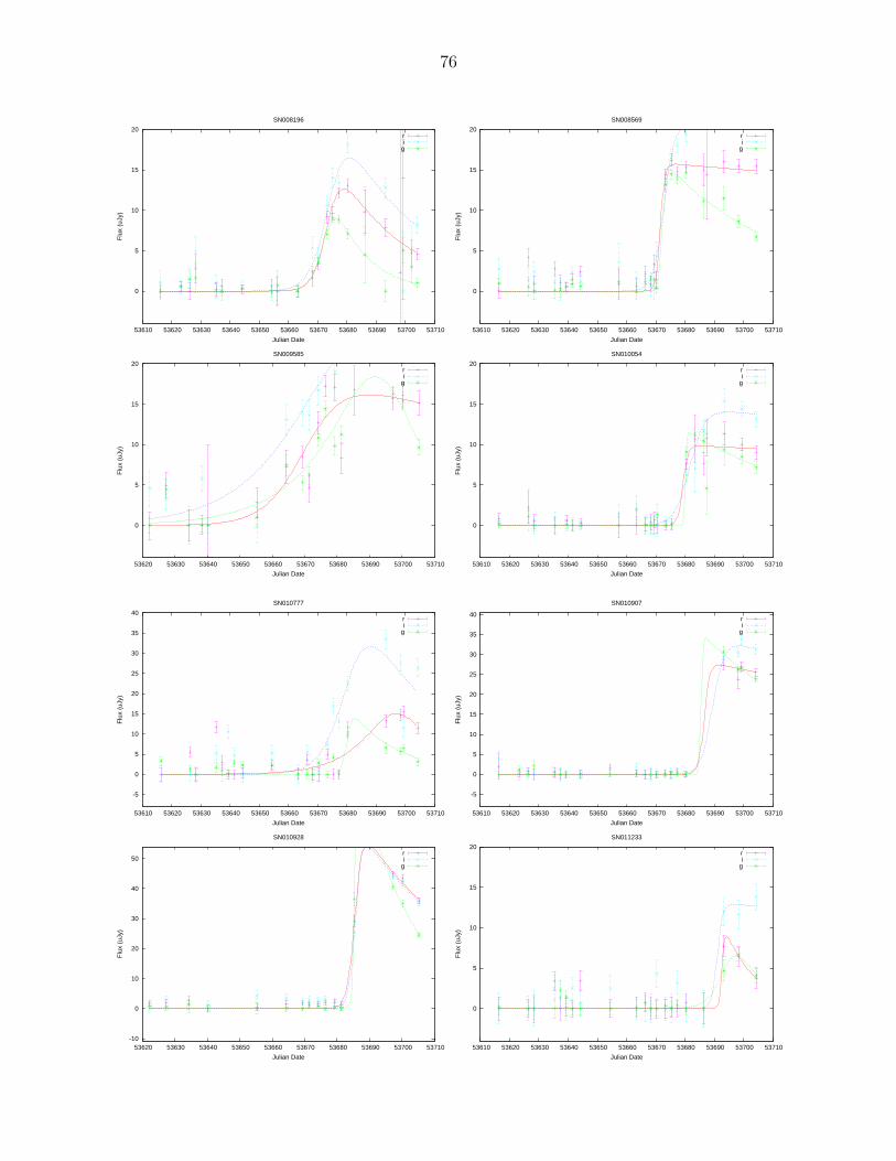
76
0
5
10
15
20
53610 53620 53630 53640 53650 53660 53670 53680 53690 53700 53710
Flu
x (u
Jy)
Julian Date
SN008196
ri
g
0
5
10
15
20
53610 53620 53630 53640 53650 53660 53670 53680 53690 53700 53710
Flu
x (u
Jy)
Julian Date
SN008569
ri
g
0
5
10
15
20
53620 53630 53640 53650 53660 53670 53680 53690 53700 53710
Flu
x (u
Jy)
Julian Date
SN009585
ri
g
0
5
10
15
20
53610 53620 53630 53640 53650 53660 53670 53680 53690 53700 53710
Flu
x (u
Jy)
Julian Date
SN010054
ri
g
-5
0
5
10
15
20
25
30
35
40
53610 53620 53630 53640 53650 53660 53670 53680 53690 53700 53710
Flu
x (u
Jy)
Julian Date
SN010777
ri
g
-5
0
5
10
15
20
25
30
35
40
53610 53620 53630 53640 53650 53660 53670 53680 53690 53700 53710
Flu
x (u
Jy)
Julian Date
SN010907
ri
g
-10
0
10
20
30
40
50
53620 53630 53640 53650 53660 53670 53680 53690 53700 53710
Flu
x (u
Jy)
Julian Date
SN010928
ri
g
0
5
10
15
20
53610 53620 53630 53640 53650 53660 53670 53680 53690 53700 53710
Flu
x (u
Jy)
Julian Date
SN011233
ri
g
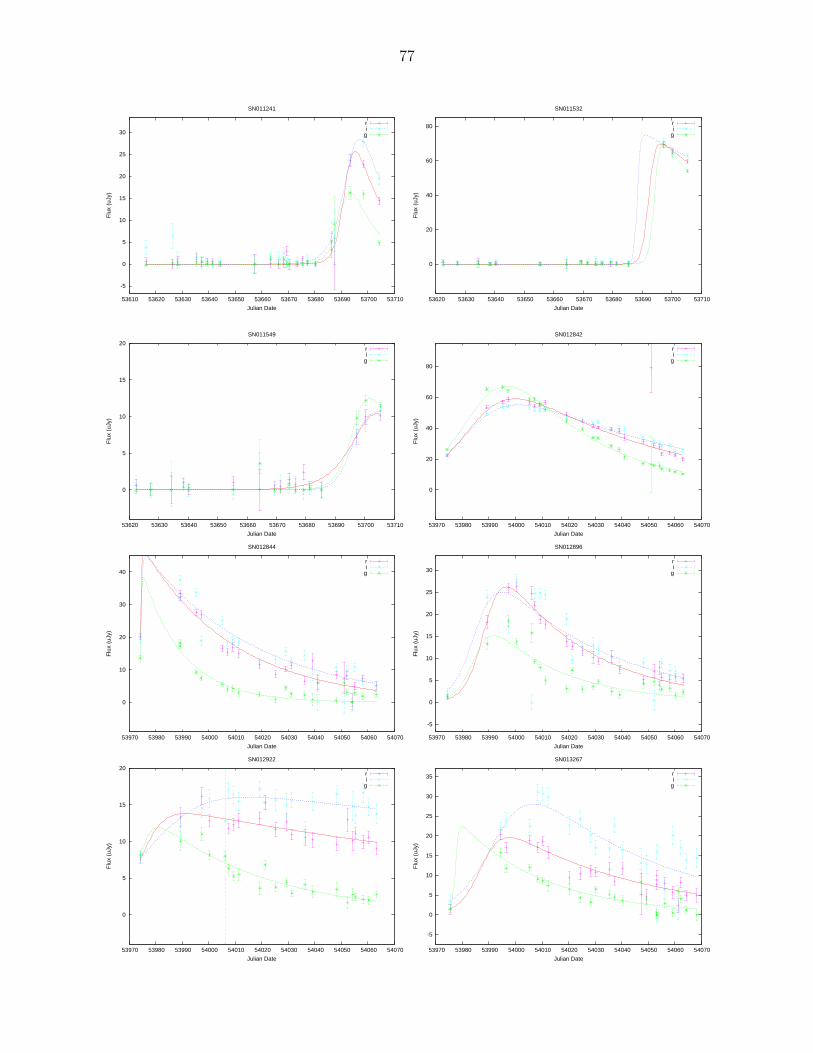
77
-5
0
5
10
15
20
25
30
53610 53620 53630 53640 53650 53660 53670 53680 53690 53700 53710
Flu
x (u
Jy)
Julian Date
SN011241
ri
g
0
20
40
60
80
53620 53630 53640 53650 53660 53670 53680 53690 53700 53710
Flu
x (u
Jy)
Julian Date
SN011532
ri
g
0
5
10
15
20
53620 53630 53640 53650 53660 53670 53680 53690 53700 53710
Flu
x (u
Jy)
Julian Date
SN011549
ri
g
0
20
40
60
80
53970 53980 53990 54000 54010 54020 54030 54040 54050 54060 54070
Flu
x (u
Jy)
Julian Date
SN012842
ri
g
0
10
20
30
40
53970 53980 53990 54000 54010 54020 54030 54040 54050 54060 54070
Flu
x (u
Jy)
Julian Date
SN012844
ri
g
-5
0
5
10
15
20
25
30
53970 53980 53990 54000 54010 54020 54030 54040 54050 54060 54070
Flu
x (u
Jy)
Julian Date
SN012896
ri
g
0
5
10
15
20
53970 53980 53990 54000 54010 54020 54030 54040 54050 54060 54070
Flu
x (u
Jy)
Julian Date
SN012922
ri
g
-5
0
5
10
15
20
25
30
35
53970 53980 53990 54000 54010 54020 54030 54040 54050 54060 54070
Flu
x (u
Jy)
Julian Date
SN013267
ri
g
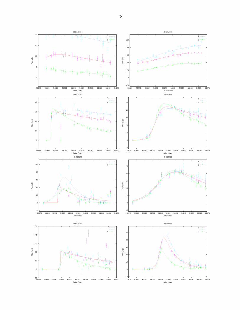
78
0
5
10
15
20
53980 53990 54000 54010 54020 54030 54040 54050 54060 54070
Flu
x (u
Jy)
Julian Date
SN013315
ri
g
-20
0
20
40
60
80
100
53980 53990 54000 54010 54020 54030 54040 54050 54060 54070
Flu
x (u
Jy)
Julian Date
SN013355
ri
g
0
10
20
30
40
53980 53990 54000 54010 54020 54030 54040 54050 54060 54070
Flu
x (u
Jy)
Julian Date
SN013376
ri
g
-10
0
10
20
30
40
50
53970 53980 53990 54000 54010 54020 54030 54040 54050 54060 54070
Flu
x (u
Jy)
Julian Date
SN013449
ri
g
-20
0
20
40
60
80
100
53970 53980 53990 54000 54010 54020 54030 54040 54050 54060 54070
Flu
x (u
Jy)
Julian Date
SN013468
ri
g
-5
0
5
10
15
20
25
53970 53980 53990 54000 54010 54020 54030 54040 54050 54060 54070
Flu
x (u
Jy)
Julian Date
SN013722
ri
g
-10
0
10
20
30
40
50
53970 53980 53990 54000 54010 54020 54030 54040 54050 54060 54070
Flu
x (u
Jy)
Julian Date
SN014030
ri
g
-10
0
10
20
30
40
50
53970 53980 53990 54000 54010 54020 54030 54040 54050 54060 54070
Flu
x (u
Jy)
Julian Date
SN014492
ri
g
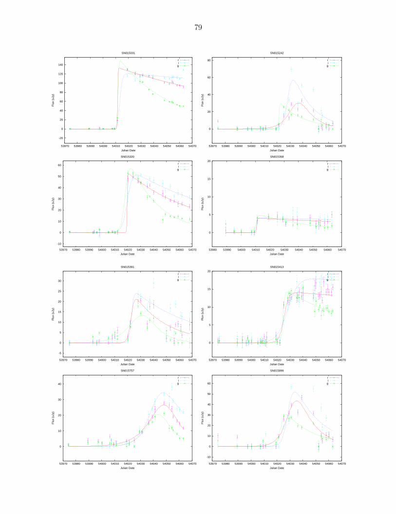
79
-20
0
20
40
60
80
100
120
140
53970 53980 53990 54000 54010 54020 54030 54040 54050 54060 54070
Flu
x (u
Jy)
Julian Date
SN015031
ri
g
0
20
40
60
80
53970 53980 53990 54000 54010 54020 54030 54040 54050 54060 54070
Flu
x (u
Jy)
Julian Date
SN015242
ri
g
-10
0
10
20
30
40
50
60
53970 53980 53990 54000 54010 54020 54030 54040 54050 54060 54070
Flu
x (u
Jy)
Julian Date
SN015320
ri
g
0
5
10
15
20
53980 53990 54000 54010 54020 54030 54040 54050 54060 54070
Flu
x (u
Jy)
Julian Date
SN015358
ri
g
-5
0
5
10
15
20
25
30
53970 53980 53990 54000 54010 54020 54030 54040 54050 54060 54070
Flu
x (u
Jy)
Julian Date
SN015391
ri
g
0
5
10
15
20
53970 53980 53990 54000 54010 54020 54030 54040 54050 54060 54070
Flu
x (u
Jy)
Julian Date
SN015413
ri
g
0
10
20
30
40
53970 53980 53990 54000 54010 54020 54030 54040 54050 54060 54070
Flu
x (u
Jy)
Julian Date
SN015757
ri
g
-10
0
10
20
30
40
50
60
53970 53980 53990 54000 54010 54020 54030 54040 54050 54060 54070
Flu
x (u
Jy)
Julian Date
SN015899
ri
g
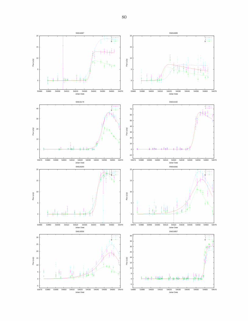
80
0
5
10
15
20
53980 53990 54000 54010 54020 54030 54040 54050 54060 54070
Flu
x (u
Jy)
Julian Date
SN016087
ri
g
0
5
10
15
20
53980 53990 54000 54010 54020 54030 54040 54050 54060 54070
Flu
x (u
Jy)
Julian Date
SN016089
ri
g
0
10
20
30
40
53970 53980 53990 54000 54010 54020 54030 54040 54050 54060 54070
Flu
x (u
Jy)
Julian Date
SN016179
ri
g
-10
0
10
20
30
40
50
60
70
53970 53980 53990 54000 54010 54020 54030 54040 54050 54060 54070
Flu
x (u
Jy)
Julian Date
SN016192
ri
0
5
10
15
20
53980 53990 54000 54010 54020 54030 54040 54050 54060 54070
Flu
x (u
Jy)
Julian Date
SN016200
ri
g
0
5
10
15
20
53970 53980 53990 54000 54010 54020 54030 54040 54050 54060 54070
Flu
x (u
Jy)
Julian Date
SN016282
ri
g
-5
0
5
10
15
20
25
30
53970 53980 53990 54000 54010 54020 54030 54040 54050 54060 54070
Flu
x (u
Jy)
Julian Date
SN016556
ri
g
-5
0
5
10
15
20
25
30
35
40
53980 53990 54000 54010 54020 54030 54040 54050 54060 54070
Flu
x (u
Jy)
Julian Date
SN016857
ri
g
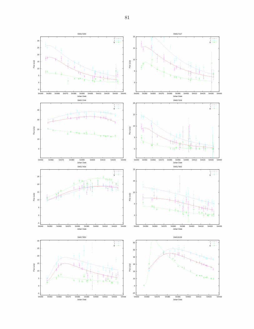
81
-5
0
5
10
15
20
25
30
54340 54350 54360 54370 54380 54390 54400 54410 54420 54430 54440
Flu
x (u
Jy)
Julian Date
SN017200
ri
g
0
5
10
15
20
54340 54350 54360 54370 54380 54390 54400 54410 54420 54430 54440
Flu
x (u
Jy)
Julian Date
SN017217
ri
g
0
10
20
30
40
54350 54360 54370 54380 54390 54400 54410 54420 54430
Flu
x (u
Jy)
Julian Date
SN017244
ri
g
0
5
10
15
20
54340 54350 54360 54370 54380 54390 54400 54410 54420 54430 54440
Flu
x (u
Jy)
Julian Date
SN017319
ri
g
-5
0
5
10
15
20
25
54340 54350 54360 54370 54380 54390 54400 54410 54420 54430
Flu
x (u
Jy)
Julian Date
SN017454
ri
g
0
5
10
15
20
54340 54350 54360 54370 54380 54390 54400 54410 54420 54430
Flu
x (u
Jy)
Julian Date
SN017663
ri
g
-5
0
5
10
15
20
25
30
54340 54350 54360 54370 54380 54390 54400 54410 54420 54430
Flu
x (u
Jy)
Julian Date
SN017953
ri
g
-10
0
10
20
30
40
50
60
54350 54360 54370 54380 54390 54400 54410 54420 54430
Flu
x (u
Jy)
Julian Date
SN018109
ri
g
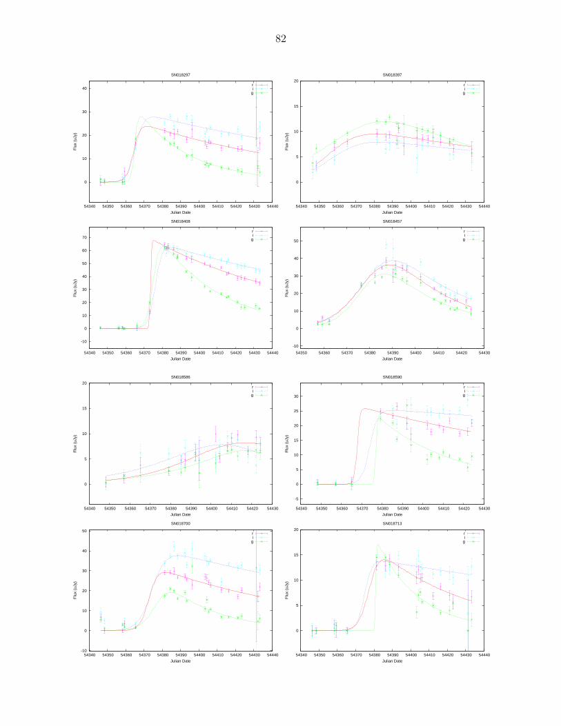
82
0
10
20
30
40
54340 54350 54360 54370 54380 54390 54400 54410 54420 54430 54440
Flu
x (u
Jy)
Julian Date
SN018297
ri
g
0
5
10
15
20
54340 54350 54360 54370 54380 54390 54400 54410 54420 54430 54440
Flu
x (u
Jy)
Julian Date
SN018397
ri
g
-10
0
10
20
30
40
50
60
70
54340 54350 54360 54370 54380 54390 54400 54410 54420 54430 54440
Flu
x (u
Jy)
Julian Date
SN018408
ri
g
-10
0
10
20
30
40
50
54350 54360 54370 54380 54390 54400 54410 54420 54430
Flu
x (u
Jy)
Julian Date
SN018457
ri
g
0
5
10
15
20
54340 54350 54360 54370 54380 54390 54400 54410 54420 54430
Flu
x (u
Jy)
Julian Date
SN018586
ri
g
-5
0
5
10
15
20
25
30
54340 54350 54360 54370 54380 54390 54400 54410 54420 54430
Flu
x (u
Jy)
Julian Date
SN018590
ri
g
-10
0
10
20
30
40
50
54340 54350 54360 54370 54380 54390 54400 54410 54420 54430 54440
Flu
x (u
Jy)
Julian Date
SN018700
ri
g
0
5
10
15
20
54340 54350 54360 54370 54380 54390 54400 54410 54420 54430 54440
Flu
x (u
Jy)
Julian Date
SN018713
ri
g
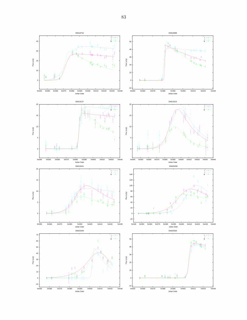
83
0
10
20
30
40
54340 54350 54360 54370 54380 54390 54400 54410 54420 54430 54440
Flu
x (u
Jy)
Julian Date
SN018734
ri
g
-10
0
10
20
30
40
50
54350 54360 54370 54380 54390 54400 54410 54420 54430
Flu
x (u
Jy)
Julian Date
SN018898
ri
g
0
5
10
15
20
54340 54350 54360 54370 54380 54390 54400 54410 54420 54430
Flu
x (u
Jy)
Julian Date
SN019137
ri
g
0
5
10
15
20
54340 54350 54360 54370 54380 54390 54400 54410 54420 54430 54440
Flu
x (u
Jy)
Julian Date
SN019323
ri
g
0
5
10
15
20
54350 54360 54370 54380 54390 54400 54410 54420 54430
Flu
x (u
Jy)
Julian Date
SN019441
ri
g
-20
0
20
40
60
80
100
120
140
54340 54350 54360 54370 54380 54390 54400 54410 54420 54430 54440
Flu
x (u
Jy)
Julian Date
SN020259
ri
g
-10
0
10
20
30
40
50
60
70
54350 54360 54370 54380 54390 54400 54410 54420 54430
Flu
x (u
Jy)
Julian Date
SN020449
ri
g
-10
0
10
20
30
40
50
54350 54360 54370 54380 54390 54400 54410 54420 54430
Flu
x (u
Jy)
Julian Date
SN020530
ri
g
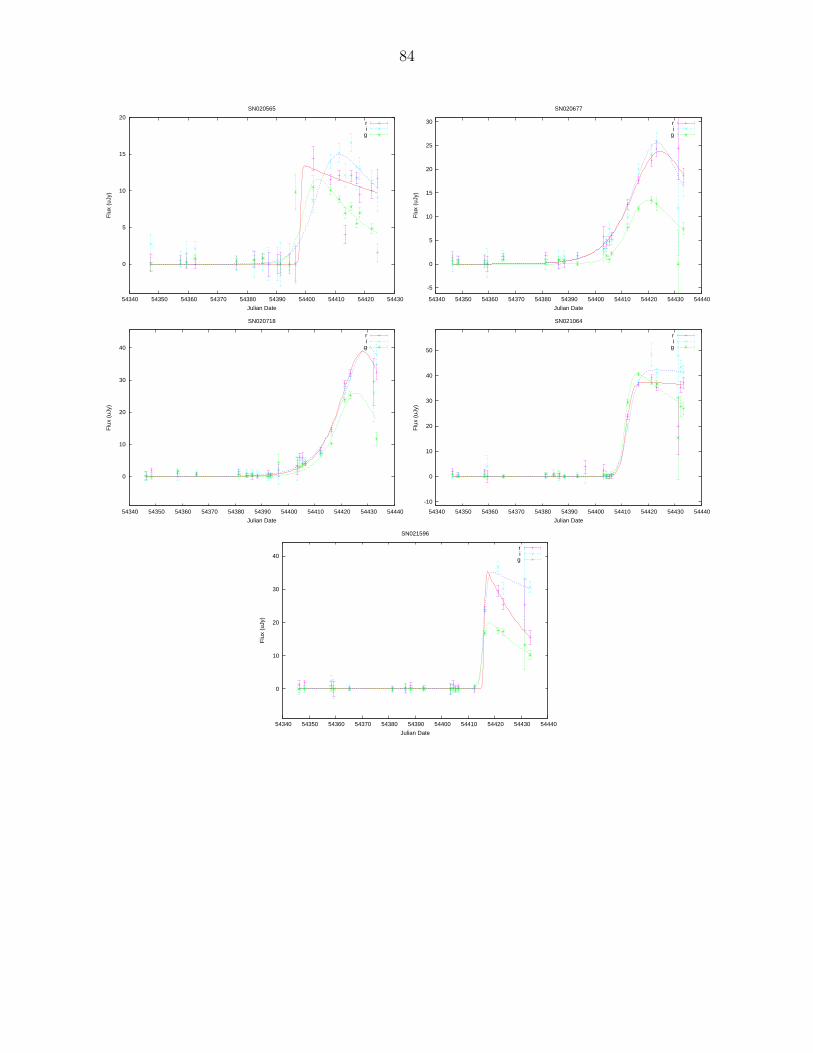
84
0
5
10
15
20
54340 54350 54360 54370 54380 54390 54400 54410 54420 54430
Flu
x (u
Jy)
Julian Date
SN020565
ri
g
-5
0
5
10
15
20
25
30
54340 54350 54360 54370 54380 54390 54400 54410 54420 54430 54440
Flu
x (u
Jy)
Julian Date
SN020677
ri
g
0
10
20
30
40
54340 54350 54360 54370 54380 54390 54400 54410 54420 54430 54440
Flu
x (u
Jy)
Julian Date
SN020718
ri
g
-10
0
10
20
30
40
50
54340 54350 54360 54370 54380 54390 54400 54410 54420 54430 54440
Flu
x (u
Jy)
Julian Date
SN021064
ri
g
0
10
20
30
40
54340 54350 54360 54370 54380 54390 54400 54410 54420 54430 54440
Flu
x (u
Jy)
Julian Date
SN021596
ri
g
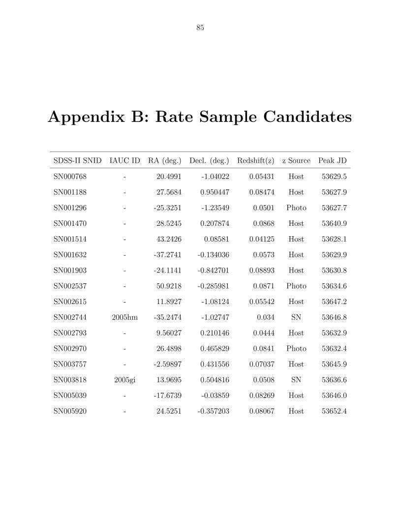
85
Appendix B: Rate Sample Candidates
SDSS-II SNID IAUC ID RA (deg.) Decl. (deg.) Redshift(z) z Source Peak JD
SN000768 - 20.4991 -1.04022 0.05431 Host 53629.5
SN001188 - 27.5684 0.950447 0.08474 Host 53627.9
SN001296 - -25.3251 -1.23549 0.0501 Photo 53627.7
SN001470 - 28.5245 0.207874 0.0868 Host 53640.9
SN001514 - 43.2426 0.08581 0.04125 Host 53628.1
SN001632 - -37.2741 -0.134036 0.0573 Host 53629.9
SN001903 - -24.1141 -0.842701 0.08893 Host 53630.8
SN002537 - 50.9218 -0.285981 0.0871 Photo 53634.6
SN002615 - 11.8927 -1.08124 0.05542 Host 53647.2
SN002744 2005hm -35.2474 -1.02747 0.034 SN 53646.8
SN002793 - 9.56027 0.210146 0.0444 Host 53632.9
SN002970 - 26.4898 0.465829 0.0841 Photo 53632.4
SN003757 - -2.59897 0.431556 0.07037 Host 53645.9
SN003818 2005gi 13.9695 0.504816 0.0508 SN 53636.6
SN005039 - -17.6739 -0.03859 0.08269 Host 53646.0
SN005920 - 24.5251 -0.357203 0.08067 Host 53652.4
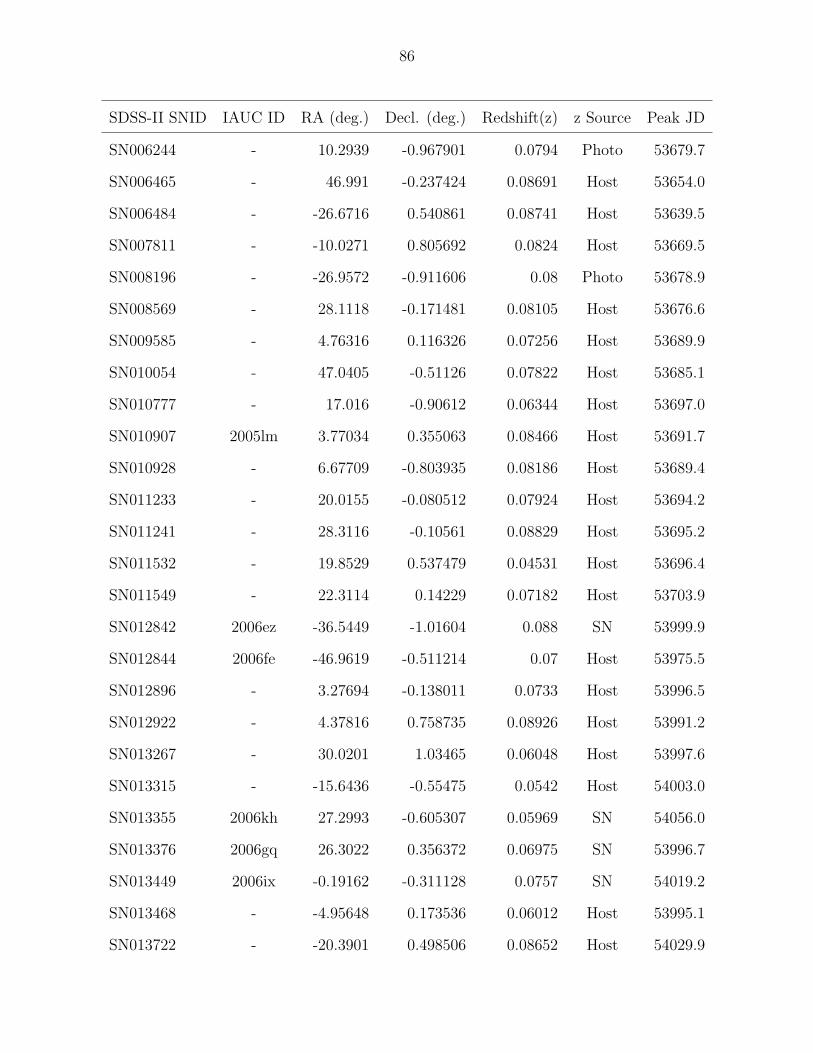
86
SDSS-II SNID IAUC ID RA (deg.) Decl. (deg.) Redshift(z) z Source Peak JD
SN006244 - 10.2939 -0.967901 0.0794 Photo 53679.7
SN006465 - 46.991 -0.237424 0.08691 Host 53654.0
SN006484 - -26.6716 0.540861 0.08741 Host 53639.5
SN007811 - -10.0271 0.805692 0.0824 Host 53669.5
SN008196 - -26.9572 -0.911606 0.08 Photo 53678.9
SN008569 - 28.1118 -0.171481 0.08105 Host 53676.6
SN009585 - 4.76316 0.116326 0.07256 Host 53689.9
SN010054 - 47.0405 -0.51126 0.07822 Host 53685.1
SN010777 - 17.016 -0.90612 0.06344 Host 53697.0
SN010907 2005lm 3.77034 0.355063 0.08466 Host 53691.7
SN010928 - 6.67709 -0.803935 0.08186 Host 53689.4
SN011233 - 20.0155 -0.080512 0.07924 Host 53694.2
SN011241 - 28.3116 -0.10561 0.08829 Host 53695.2
SN011532 - 19.8529 0.537479 0.04531 Host 53696.4
SN011549 - 22.3114 0.14229 0.07182 Host 53703.9
SN012842 2006ez -36.5449 -1.01604 0.088 SN 53999.9
SN012844 2006fe -46.9619 -0.511214 0.07 Host 53975.5
SN012896 - 3.27694 -0.138011 0.0733 Host 53996.5
SN012922 - 4.37816 0.758735 0.08926 Host 53991.2
SN013267 - 30.0201 1.03465 0.06048 Host 53997.6
SN013315 - -15.6436 -0.55475 0.0542 Host 54003.0
SN013355 2006kh 27.2993 -0.605307 0.05969 SN 54056.0
SN013376 2006gq 26.3022 0.356372 0.06975 SN 53996.7
SN013449 2006ix -0.19162 -0.311128 0.0757 SN 54019.2
SN013468 - -4.95648 0.173536 0.06012 Host 53995.1
SN013722 - -20.3901 0.498506 0.08652 Host 54029.9
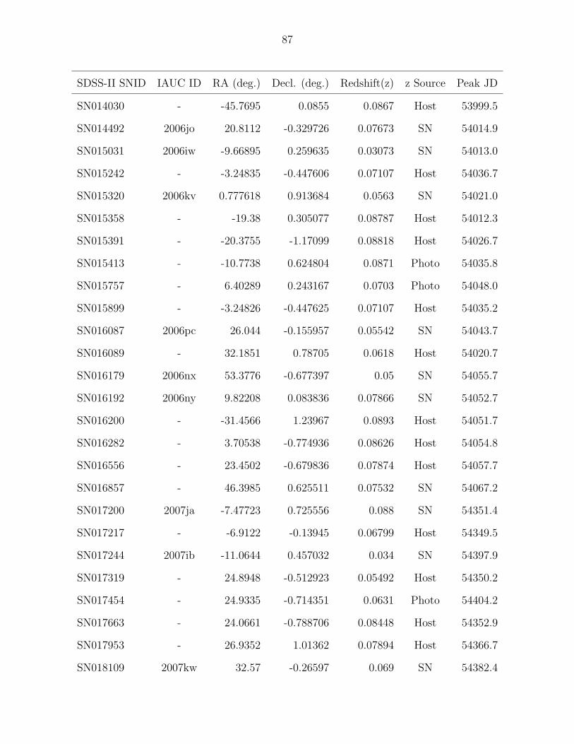
87
SDSS-II SNID IAUC ID RA (deg.) Decl. (deg.) Redshift(z) z Source Peak JD
SN014030 - -45.7695 0.0855 0.0867 Host 53999.5
SN014492 2006jo 20.8112 -0.329726 0.07673 SN 54014.9
SN015031 2006iw -9.66895 0.259635 0.03073 SN 54013.0
SN015242 - -3.24835 -0.447606 0.07107 Host 54036.7
SN015320 2006kv 0.777618 0.913684 0.0563 SN 54021.0
SN015358 - -19.38 0.305077 0.08787 Host 54012.3
SN015391 - -20.3755 -1.17099 0.08818 Host 54026.7
SN015413 - -10.7738 0.624804 0.0871 Photo 54035.8
SN015757 - 6.40289 0.243167 0.0703 Photo 54048.0
SN015899 - -3.24826 -0.447625 0.07107 Host 54035.2
SN016087 2006pc 26.044 -0.155957 0.05542 SN 54043.7
SN016089 - 32.1851 0.78705 0.0618 Host 54020.7
SN016179 2006nx 53.3776 -0.677397 0.05 SN 54055.7
SN016192 2006ny 9.82208 0.083836 0.07866 SN 54052.7
SN016200 - -31.4566 1.23967 0.0893 Host 54051.7
SN016282 - 3.70538 -0.774936 0.08626 Host 54054.8
SN016556 - 23.4502 -0.679836 0.07874 Host 54057.7
SN016857 - 46.3985 0.625511 0.07532 SN 54067.2
SN017200 2007ja -7.47723 0.725556 0.088 SN 54351.4
SN017217 - -6.9122 -0.13945 0.06799 Host 54349.5
SN017244 2007ib -11.0644 0.457032 0.034 SN 54397.9
SN017319 - 24.8948 -0.512923 0.05492 Host 54350.2
SN017454 - 24.9335 -0.714351 0.0631 Photo 54404.2
SN017663 - 24.0661 -0.788706 0.08448 Host 54352.9
SN017953 - 26.9352 1.01362 0.07894 Host 54366.7
SN018109 2007kw 32.57 -0.26597 0.069 SN 54382.4
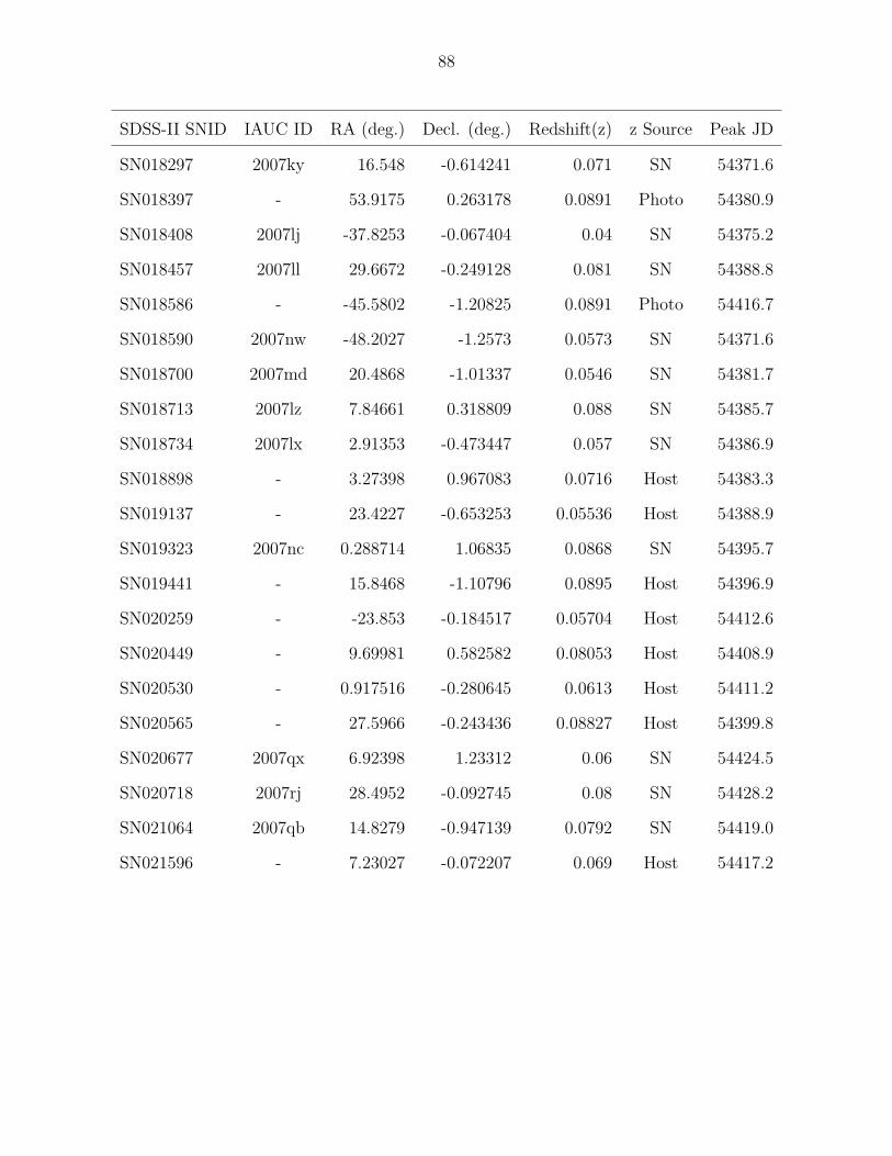
88
SDSS-II SNID IAUC ID RA (deg.) Decl. (deg.) Redshift(z) z Source Peak JD
SN018297 2007ky 16.548 -0.614241 0.071 SN 54371.6
SN018397 - 53.9175 0.263178 0.0891 Photo 54380.9
SN018408 2007lj -37.8253 -0.067404 0.04 SN 54375.2
SN018457 2007ll 29.6672 -0.249128 0.081 SN 54388.8
SN018586 - -45.5802 -1.20825 0.0891 Photo 54416.7
SN018590 2007nw -48.2027 -1.2573 0.0573 SN 54371.6
SN018700 2007md 20.4868 -1.01337 0.0546 SN 54381.7
SN018713 2007lz 7.84661 0.318809 0.088 SN 54385.7
SN018734 2007lx 2.91353 -0.473447 0.057 SN 54386.9
SN018898 - 3.27398 0.967083 0.0716 Host 54383.3
SN019137 - 23.4227 -0.653253 0.05536 Host 54388.9
SN019323 2007nc 0.288714 1.06835 0.0868 SN 54395.7
SN019441 - 15.8468 -1.10796 0.0895 Host 54396.9
SN020259 - -23.853 -0.184517 0.05704 Host 54412.6
SN020449 - 9.69981 0.582582 0.08053 Host 54408.9
SN020530 - 0.917516 -0.280645 0.0613 Host 54411.2
SN020565 - 27.5966 -0.243436 0.08827 Host 54399.8
SN020677 2007qx 6.92398 1.23312 0.06 SN 54424.5
SN020718 2007rj 28.4952 -0.092745 0.08 SN 54428.2
SN021064 2007qb 14.8279 -0.947139 0.0792 SN 54419.0
SN021596 - 7.23027 -0.072207 0.069 Host 54417.2
89
BIBLIOGRAPHY
[1] G. Bazin et al., Astronomy and Astrophysics 499, 653 (2009).
[2] Paul Murdin and Lesley Murdin, Supernovae. Cambridge University Press (1985).
[3] Retrieved from http://www.cfa.harvard.edu/iau/nova list.html, December 6,
2010.
[4] P. Filippenko et al, Annual Review of Astronomy and Astrophysics 36, 309 (1997).
[5] L. Bildsten et al., The Astrophysical Journal 662, L95 (2007).
[6] Dina Prialnik, An Introduction to the Theory of Stellar Structure and Evolution. Cam-
bridge University Press (2008).
[7] W.N. Cottingham and D.A. Greenwood, An Introduction to Nuclear Physics. Cambridge
University Press (2004).
[8] Retrieved from http://apod.nasa.gov/apod/ap051202.html, December 6, 2010.
[9] A. Hewish and S.E. Okoye, Nature 207, 59 (1965).
[10] W. Baade and F. Zwicky, The Physical Review 46, 76 (1934).
[11] V. Trimble, Reviews of Modern Physics 54, 1183 (1982).
[12] E. Cappellaro et al., Astronomy and Astrophysics 351, 459 (1999).
[13] T. Dahlen et al., The Astrophysical Journal 613, 189 (2004).
[14] F. Mannucci et al., Astronomy and Astrophysics 433, 807 (2005).
[15] M. Botticella et al., Astronomy and Astrophysics 479, 49 (2008).
90
[16] Retrieved from http://www.sdss.org, October 21, 2010.
[17] J. Gunn et al., The Astronomical Journal 116, 3040 (1998).
[18] D. York et al., The Astrophysical Journal 120, 1579 (2000).
[19] L. Girardi et al., Astronomy and Astrophysics 391, 195 (2002).
[20] J. Frieman et al., The Astronomical Journal 135, 338 (2008).
[21] R. Kessler et al., The Astrophysical Journal Supplement Series 185, 32 (2009).
[22] J. Guy et al, Astronomy and Astrophysics 466, 11 (2007).
[23] B. Dilday et al., The Astrophysical Journal 713, 1026 (2010).
[24] D. Schlegel et al., The Baryon Oscillation Spectroscopic Survey: Precision Measure-
ments of the Absolute Cosmic Distance Scale. White Paper for the Astro2010 CFP
Science Frontier Panel (2009).
[25] B. Dilday et al., The Astrophysical Journal 682, 262 (2008).
[26] R. Lupton et al, ASP Conf. Ser. 238, Astronomical Data Analysis Software and Systems
(San Francisco:ASP), 269 (2001).
[27] G. Miknaitis et al, Bulletin of the American Astronomical Society 34, 1205 (2002).
[28] B. Basset et al, SDSS-II SN Super-unofficial Hand-Scanning Guide, Retrieved from
http://sdssdp62.fnal.gov/sdsssn data/sdsssn.html, April 1, 2011.
[29] J. Holtzman et al, The Astronomical Journal 136, 2306 (2008).
[30] Joachim Wuttke: lmfit - a C/C++ routine for Levenberg-Marquardt minimization with
wrapper for least-squares curve fitting, based on work by B. S. Garbow, K. E. Hillstrom,
J. J. Morand S. Moshier. Version 2.4, retrieved on 7/27/2008 from http://www.messen-
und-deuten.de/lmfit/.
[31] M. Sako et al, The Astronomical Journal 135, 348 (2008).
[32] C. Zheng et al, The Astronomical Journal 135, 1766 (2008).
91
[33] S. Jha et al, The Astrophysical Journal 659, 122 (2007).
[34] A. Connolly et al, The Astronomical Journal, 110, 2665 (1995).
[35] L. da Costa et al, The Astrophysical Journal Letters 424, L1 (1994).
[36] David W. Hogg, arXiv:9905116 [astro-ph] (2000).
[37] M. Vardanyan, iCosmos Cosmology Calculator, Retrieved from
http://www.icosmos.co.uk, April 10, 2011.
[38] J. Cardelli et al, The Astrophysical Journal 345, 245 (1989).
[39] K. Hatano et al, The Astrophysical Journal 502, 177 (1998).
[40] Shunsaku Horiuchi et al, arXiv:1102.1977 [astro-ph] (2011).
[41] I. Baldry et al, Monthly Notices of the Royal Astronomical Society 358, 441 (2005).
[42] R. Nave, Stellar Lifetime Calculator, Retrieved from
http://hyperphysics.phy-astr.gsu.edu/hbase/astro/startime.html, May 1,
2011.
[43] J. Anthony, Large Synoptic Survey Telescope - Overview, Proceedings of SPIE 4836,
10 (2002).
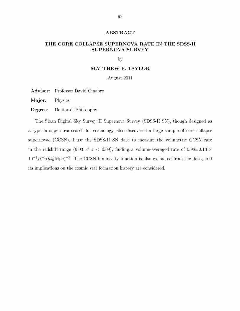
92
ABSTRACT
THE CORE COLLAPSE SUPERNOVA RATE IN THE SDSS-IISUPERNOVA SURVEY
by
MATTHEW F. TAYLOR
August 2011
Advisor: Professor David Cinabro
Major: Physics
Degree: Doctor of Philosophy
The Sloan Digital Sky Survey II Supernova Survey (SDSS-II SN), though designed as
a type Ia supernova search for cosmology, also discovered a large sample of core collapse
supernovae (CCSN). I use the SDSS-II SN data to measure the volumetric CCSN rate
in the redshift range (0.03 < z < 0.09), finding a volume-averaged rate of 0.98±0.18 ×
10−4yr−1(h−170 Mpc)−3. The CCSN luminosity function is also extracted from the data, and
its implications on the cosmic star formation history are considered.
93
Autobiographical Statement
Name: Matthew F. Taylor
Education:M.S. Applied Physics, Rice University, Houston, Texas, 2001B.S. Computer Science, University of Michigan, Ann Arbor, Michigan, 1989Professional Experience:Software Engineer, Cray Inc., Mendota Heights, Minnesota, 2003-2005Software Engineer, Hewlett-Packard, Houston, Texas, 2001-2003Software Engineer, Lucent Technologies, Naperville, Illinois, 1989-1997Publications:“SNANA: A Public Software Package for Supernova Analysis,” Publications of the Astro-nomical Society of the Pacific v. 121, p. 1028 (2009)“Electron Tunneling Rates between an Atom and a Corrugated Surface,” Physical ReviewB v. 64, p. 115422 (2001)
From a very young age I have always had a strong interest in mathematics in science.Like many people with similar interests, I was initially drawn to the field of informationtechnology, which was relatively new in the late 1980’s when I began my career. Aftercompleting my Bachelor’s in computer science, I worked for several years as a softwareengineer for ATT (later called Lucent Technologies) in the Chicago area.
While software development is a rewarding and interesting pursuit, I came to realizethat I have an especially deep interest in the physical sciences and that a deeper study ofphysics in particular is an essential life goal for me. Therefore, I eventually left the softwaredevelopmebt field and enrolled in a graduate Applied Physics program at Rice University,in Houston, Texas. At Rice, I concentrated on the study of quantum mechanics, atomic andmolecular physics, and condensed matter physics. After completing my Master’s at Rice, Ireturned to the private sector as a software developer once again.
A few more years of work passed, this time for Compaq in Houston, Texas (now a divisionof Hewlett-Packard), and then for Cray Inc. in Minnesota. Though my work in informationtechnology was interesting and rewarding, as always, I again found myself drawn to gain adeeper understanding of physics. This time I was most interested in studying topics withinphysics that I had only lightly touched on at Rice, namely nuclear physics, elementaryparticles, astrophysics and cosmology. I therefore applied to the WSU PhD physics program.At WSU, I participated in theoretical nuclear physics research with Prof. Sean Gavin., andthen astrophysics and cosmology with Prof Cinabro.
Working here at WSU, I have also discovered an unexpected interest in and aptitude foreducation. I have found it especially rewarding to help students who find math and sciencedifficult learn about these topics, in spite of their initial aversion and confusion. Perhapsthis will lead me toward a new career path in education. I have certainly enjoyed learningabout every aspect of physics throughout my studies; it would be rewarding to share thatknowledge and the enjoyment of it with future students.