the core of fse-cma behavior theory1schniter/pdf/haykin_chapter.pdf · the core of fse-cma behavior...
TRANSCRIPT
The Core of FSE-CMA Behavior Theory 1
The Core of FSE-CMA Behavior Theory1
C.R. Johnson, Jr., P. Schniter, I. Fijalkow, L. Tong,
J.D. Behm, M.G. Larimore,
D.R. Brown, R.A. Casas, T.J. Endres, S. Lambotharan,
A. Touzni, H.H. Zeng, M. Green, and J.R. Treichler
Abstract
This chapter presents the basics of the current theory regarding the behavior of blind fractionally-spaced and/or
spatial-diversity equalizers (FSE) adapted via the constant modulus algorithm (CMA). The constant modulus algo-
rithm, which was developed in the late 1970s and disclosed in the early 1980s, performs a stochastic gradient descent
of a cost function that penalizes the dispersion of the equalizer output from a constant value. The constant modulus
(CM) cost function leads to a blind algorithm because evaluation of the CM cost at the receiver does not rely on
access to a replica of the transmitted source, as in so-called “trained” scenarios. The capability for blind start-up
makes certain communication systems feasible in circumstances that do not admit training. The analytically conve-
nient feature of the fractionally-spaced realization of a linear equalizer is the potential for perfect equalization in the
absence of channel noise given a finite impulse response equalizer of time span matching that of the finite impulse
response channel. The conditions for perfect equalization coupled with some mild conditions on the source can be
used to establish convergence to perfect performance with FSE parameter adaptation by CMA from any equalizer
parameter initialization. The FSE-CMA behavior theory presented here merges the taxonomy of the behavior theory
of trained adaptive equalization and recent robustness analysis of FSE-CMA with violation of the conditions leading
to perfect equalization and global asymptotic optimality of FSE-CMA.
1To appear as a chapter in the book Unsupervised Adaptive Filtering, Simon Haykin, ed., Wiley: New York, 1999.
2 Johnson, et al.
1.1 Introduction
The revolution in data communications technology can be dated from the invention of automatic
and adaptive channel equalization in the late 1960s... Many engineers contributed to this revolu-
tion, but the early inventions of Robert W. Lucky, particularly data-driven equalizer adaptation,
were the largest factor in realizing higher-speed data communication in commercial equipment.
[Gitlin, Hayes, and Weinstein, Data Communication Principles, 1992, p. viii]
There are several applications in digital data communications when start-up and retraining of an
adaptive equalizer has to be accomplished without the aid of a training sequence. Hence, the system
has to be trained “blind”... We are interested in those circumstances where the eye is closed, and
the conventional decision-directed operation will fail... It is recognized that, in exchange for
not requiring data decisions, blind equalization algorithms may require one or two more orders
of magnitudes of time to converge. There are two basic algorithms for blind equalization: the
constant modulus algorithm (CMA)...
[ibid, p. 585]
Motivation
The desire to move data at high rates across transmission media with limited bandwidth has prompted the
development of sophisticated communications systems, e.g., voiceband modems and microwave radio relay
systems. Success in those applications has led to great interest in other communication scenarios in which
economic or regulatory considerations limit the available transmission bandwidth. An important example of
such an application is the wireless and cable distribution of digital television.
Central to the successful employment of most high data rate transmission systems is the use of adaptive
equalization to counteract the disruptive effects of the signal’s propagation from the transmitter to the
receiver. The equalizer’s importance, coupled with the fact that it tends to consume most of the receiver’s
computational resources and implementation cost, has made it the focus of much analytical and practical
attention. Initially, high data rate communication systems utilized session-oriented point-to-point links that
accommodated cooperative equalizer training. By training, we mean the transmission of a symbol sequence
known in advance by the receiver and usually preceded by a clearly identifiable synchronization burst. The
more recent emergence of digital multi-point and broadcast systems has produced communication scenarios
where training is infeasible or prohibited. In this chapter we are interested in “blind” adaptive equalizers,
that is, those that do not need training to achieve convergence from an unacceptable equalizer setting to an
acceptable one. In a style intended for the engineer with a first-year-graduate level acquaintance with digital

The Core of FSE-CMA Behavior Theory 3
communication systems, this chapter presents the core of the behavior theory of the most popular of blind
equalization algorithms, CMA, in the so-called “fractionally-spaced” configuration that dominates current
practice. The theory chosen here was selected for its utility in illuminating pragmatic design guidelines.
History
The concept of an adaptive digital linear equalizer was introduced and realized in the 1960s. (See
[Qureshi PROC 85] for an excellent survey of pre-1985 advances in trained adaptive equalization and numer-
ous references regarding the highlights cited here.) The received signal’s sampling interval matched the baud
interval, that is, the time between transmission of consecutive source symbols. The baud-spaced equalizer
tapped-delay-line length was selected to provide an accurate delayed inverse of a mixed-phase but finite-
duration impulse response (FIR) channel. The common theoretical assumption of infinite equalizer length
can be attributed to the recognition that an infinitely long tapped-delay line would be required for perfect2
equalization of a FIR channel even in the absence of channel noise. Algorithms with and without training
were introduced in the 1960s (e.g., [Lucky BSTJ 66]). The format with training quickly dominated telephony
practice, at least for session start-up, and decision-directed LMS assumed the role of the fundamental blind
method for subsequent tracking.
The 1970s witnessed the emergence of fractionally-spaced equalizer implementations, that is, those that
used sampling rates faster than the source symbol rate. Improved band-edge equalization capabilities and
reduced sensitivity to timing synchronization errors were cited as motivation [Ungerboeck TCOM 76]. The
practical necessity of “tap leakage” for long fractionally-spaced equalizers was the most significant adap-
tive equalizer algorithm modification [Gitlin Book 92]. Performance analyses for both fractionally-spaced
and baud-spaced equalizers commonly included assumptions of effectively infinite equalizer length, which
permitted perfect equalization and easy translation between time and frequency domain interpretations.
During the 1980s, linear equalization methods capable of blind start-up moved from concept into practice.
Blind equalization is desirable in multi-point and broadcast systems and necessary in non-invasive test and
intercept scenarios. Even in point-to-point communication systems, blind equalization has been adopted for
various reasons, including capacity gain and procedural convenience. For performance reasons, fractional
spacing of the equalizer became preferred where technologically feasible. However, performance analysis of
blind equalizers remained focused almost exclusively on baud-spaced realizations [Haykin Book 94].
During the 1990s, blind equalization has been incorporated into several emerging communication tech-
nologies [Treichler SPM 96], [Treichler PROC 98], e.g., digital cable TV. Also in the 1990s, realization of
the ideal capabilities of fractionally-spaced data-adaptive equalizers, especially blind finite-length varieties
2Perfect equalization denotes situations in which the equalizer output sequence equals the transmitted symbol sequence up
to a (fixed) unknown amplitude and delay.
4 Johnson, et al.
[Tong TIT 95], have energized the study of finite-length fractionally-spaced blind equalizers. See, for exam-
ple, [Johnson PROC 98], appearing in the special issue [Liu PROC 98]. The advantages that result from
utilizing time-diversity (i.e., fractional sampling) also occur in spatial diversity systems (e.g., those employing
multiple sensors or cross polarity) and code diversity systems (e.g., short-code DS-CDMA) [Paulraj SPM 97].
Our Goal: Behavior Theory Basics and Design Guidelines
The pedagogy employed here is fundamentally similar to that used in a variety of widely cited textbooks
(e.g., [Proakis Book 95], [Gitlin Book 92], [Lee Book 94]) for trained, baud-spaced equalization theory, based
on minimization of the mean squared error (MSE) in recovery of the training sequence. This approach is
bolstered by recent results—to be described in this chapter—on the similarity of the locations of MSE minima
and minima of the (blind) constant modulus (CM) cost function. Such similarities prompt the adoption of a
taxonomy associated with design rules for trained stochastic gradient descent procedures, such as the LMS
algorithm, to a stochastic gradient descent approach for minimizing the CM cost via the constant modulus
algorithm (CMA). This results in design guidelines—to be developed and dissected in this chapter—regarding
adaptive algorithm step-size selection, equalizer length, and equalizer parameter (re)initialization.
Content Map
Against this backdrop we present a map of the contents of this chapter, carrying us from a fractionally-
spaced equalizer problem formulation to an understanding of the design guidelines for blind CMA-FSE, that
is, CMA-based adaptation of a fractionally-spaced equalizer.
• Section 10.2 introduces the fractionally-spaced equalizer problem formulation. A multichannel model
is adopted and the capability for perfect symbol recovery is established with a fractionally-spaced
equalizer in the absence of channel noise. With the addition of channel noise, the Wiener solution
(with a necessarily nonzero minimum mean-squared, delayed-source recovery error) is formulated for
an infinite-duration impulse response (IIR) linear equalizer and for a finite-duration impulse response
(FIR) linear equalizer. The resulting minimum mean-squared error is dissected in terms of its factors
(i.e., noise power, equalizer length, channel convolution matrix singular values, and target system
delay). Given a description of transient and asymptotic performance of the underlying average system
behavior, a brief distillation of step-size and equalizer length design guidelines for LMS-FSE is also
provided as the background against which CMA-FSE design guidelines will be composed.
• Section 10.3 begins with definition of the CM (or CMA 2-2) criterion and combines the perfect equal-
ization requirements with some generic assumptions on the source statistics to result in a set of re-
quirements for CMA-FSE’s global asymptotic optimality. A series of 2-tap FSE CM cost functions and

The Core of FSE-CMA Behavior Theory 5
CMA trajectories is used to illustrate the basic robustness properties with violations of each of these
conditions. Approximate perturbation analyses of the effects of channel noise and equalizer length and
a geometric analysis of the achieved MSE of a CM-minimizing equalizer in the presence of channel
noise are exploited for insight. Differences in CMA-FSE relative to LMS-FSE are highlighted with
examination of convergence rate and excess MSE.
• Section 10.4 focuses on three design choices in CMA-FSE implementation: adaptive equalizer parame-
ter update step-size, equalizer length, and equalizer parameter initialization. Guidelines are developed
through an example-driven tutorial approach. Single-spike initialization for CMA-BSE and double-
spike initialization for CMA-FSE are discussed in terms of magnitude and location. In step-size selec-
tion, the tradeoffs in LMS design (i.e., (i) between convergence rate and excess MSE and (ii) between
tracking error and gradient approximation error) are noted to drive CMA step-size selection as well.
A similar tradeoff between improved modeling accuracy and increased excess mean squared error is
discussed for increases in equalizer length.
• Section 10.5 presents three case studies, each of which yields a blind equalizer capable of dealing with a
particular problem class (specifically, voice channel modem, cable-borne HDTV, and microwave radio)
represented by signals and channel models in a publicly accessible database.
Notation
The following tables present the abbreviations and mathematical notation used throughout this chapter.

6 Johnson, et al.
Table 1.1: Acronyms and Abbreviations
Acronym Definition
BER Bit error rate
BPSK Binary phase-shift keying
BS Baud-spaced
BSE Baud-spaced equalizer
CM Constant modulus
CMA Constant modulus algorithm
DD Decision-directed
EMSE Excess mean-squared error
FIR Finite-duration impulse response
FS Fractionally-spaced
FSE Fractionally-spaced equalizer
i.i.d. Independent and identically distributed
IIR Infinite-duration impulse response
ISI Inter-symbol interference
LMS Least mean-square
MMSE Minimum mean-squared error
MSE Mean-squared error
ODE Ordinary differential equation
PAM Pulse amplitude modulation
PBE Perfect blind equalizability
pdf Probability density function
PSK Phase-shift keying
QAM Quadrature amplitude modulation
QPSK Quadrature phase-shift keying
SER Symbol error rate
SNR Signal to noise ratio
SPIB Signal Processing Information Base
SVD Singular value decomposition
ZF Zero-forcing
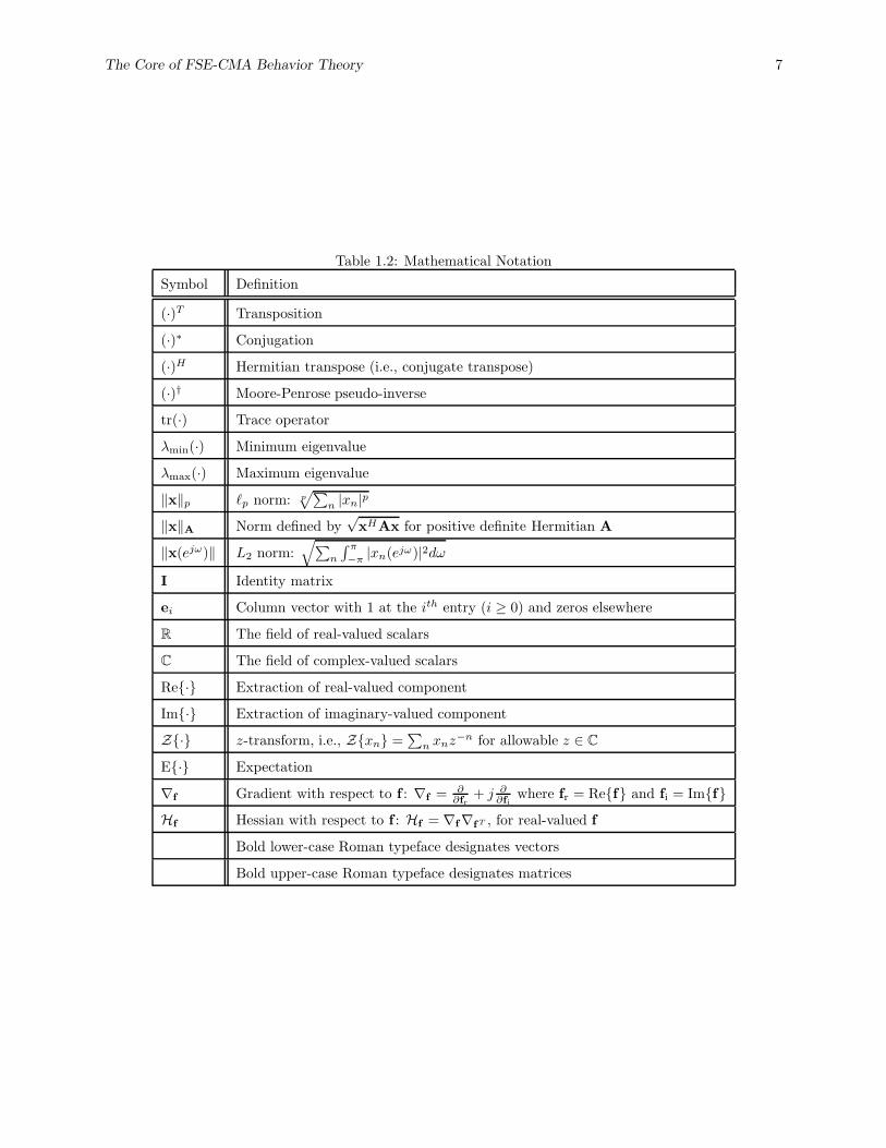
The Core of FSE-CMA Behavior Theory 7
Table 1.2: Mathematical Notation
Symbol Definition
(·)T Transposition
(·)∗ Conjugation
(·)H Hermitian transpose (i.e., conjugate transpose)
(·)† Moore-Penrose pseudo-inverse
tr(·) Trace operator
λmin(·) Minimum eigenvalue
λmax(·) Maximum eigenvalue
‖x‖p `p norm: p√∑
n |xn|p
‖x‖A Norm defined by√
xHAx for positive definite Hermitian A
‖x(ejω)‖ L2 norm:√∑
n
∫ π
−π|xn(ejω)|2dω
I Identity matrix
ei Column vector with 1 at the ith entry (i ≥ 0) and zeros elsewhere
R The field of real-valued scalars
C The field of complex-valued scalars
Re{·} Extraction of real-valued component
Im{·} Extraction of imaginary-valued component
Z{·} z-transform, i.e., Z{xn} =∑
n xnz−n for allowable z ∈ C
E{·} Expectation
∇f Gradient with respect to f : ∇f = ∂∂fr
+ j ∂∂fi
where fr = Re{f} and fi = Im{f}Hf Hessian with respect to f : Hf = ∇f∇fT , for real-valued f
Bold lower-case Roman typeface designates vectors
Bold upper-case Roman typeface designates matrices

8 Johnson, et al.
Table 1.3: System Model Quantities
Symbol Definition
T Symbol period
n Index for quantities sampled at baud intervals: t = nT
k Index for fractionally sampled quantities: t = kT/P
δ System delay (non-negative, integer-valued)
qn System impulse response coefficient
sn Source symbol
yn System/equalizer output
νn Filtered noise contribution to system output
q(z) System transfer function Z{qn}s(z) z-transformed source sequence Z{sn}y(z) z-transformed output sequence Z{yn}ν(z) z-transformed noise sequence Z{νn}q Vector of BS system response coefficients {qn}s(n) Vector of past source symbols {sn} at time n
H (Multi)channel convolution matrix
σ2s Variance of source sequence: E{|sn|2}
κs Normalized kurtosis of source process: E{|sn|4}/σ4s
κg Normalized kurtosis of a Gaussian process
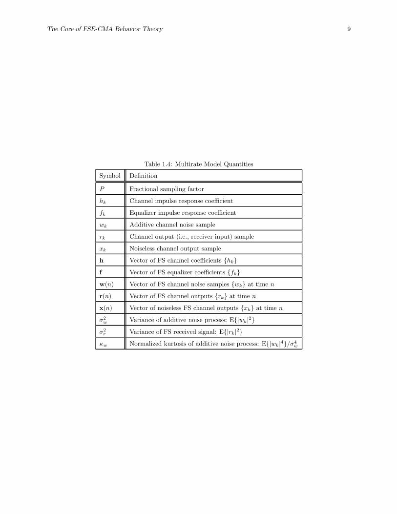
The Core of FSE-CMA Behavior Theory 9
Table 1.4: Multirate Model Quantities
Symbol Definition
P Fractional sampling factor
hk Channel impulse response coefficient
fk Equalizer impulse response coefficient
wk Additive channel noise sample
rk Channel output (i.e., receiver input) sample
xk Noiseless channel output sample
h Vector of FS channel coefficients {hk}f Vector of FS equalizer coefficients {fk}w(n) Vector of FS channel noise samples {wk} at time n
r(n) Vector of FS channel outputs {rk} at time n
x(n) Vector of noiseless FS channel outputs {xk} at time n
σ2w Variance of additive noise process: E{|wk|2}
σ2r Variance of FS received signal: E{|rk|2}
κw Normalized kurtosis of additive noise process: E{|wk|4}/σ4w
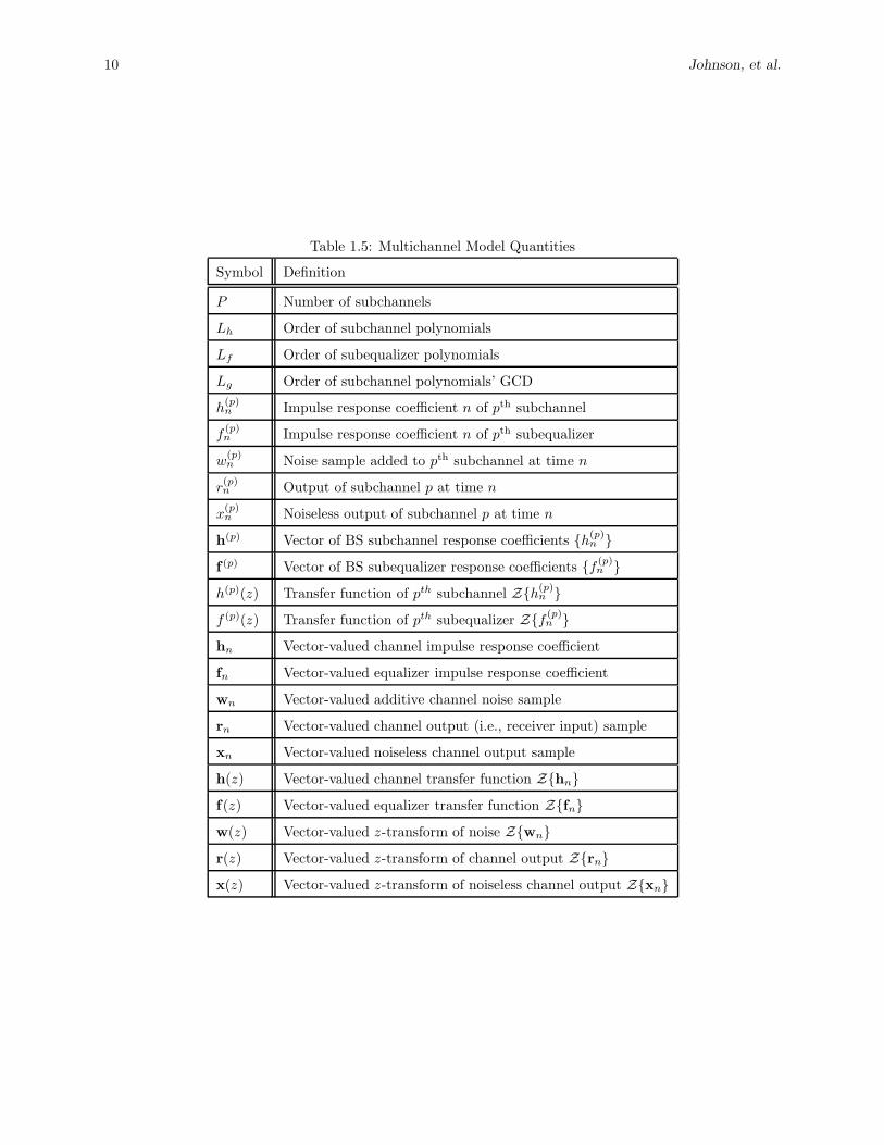
10 Johnson, et al.
Table 1.5: Multichannel Model Quantities
Symbol Definition
P Number of subchannels
Lh Order of subchannel polynomials
Lf Order of subequalizer polynomials
Lg Order of subchannel polynomials’ GCD
h(p)n Impulse response coefficient n of pth subchannel
f(p)n Impulse response coefficient n of pth subequalizer
w(p)n Noise sample added to pth subchannel at time n
r(p)n Output of subchannel p at time n
x(p)n Noiseless output of subchannel p at time n
h(p) Vector of BS subchannel response coefficients {h(p)n }
f (p) Vector of BS subequalizer response coefficients {f (p)n }
h(p)(z) Transfer function of pth subchannel Z{h(p)n }
f (p)(z) Transfer function of pth subequalizer Z{f (p)n }
hn Vector-valued channel impulse response coefficient
fn Vector-valued equalizer impulse response coefficient
wn Vector-valued additive channel noise sample
rn Vector-valued channel output (i.e., receiver input) sample
xn Vector-valued noiseless channel output sample
h(z) Vector-valued channel transfer function Z{hn}f(z) Vector-valued equalizer transfer function Z{fn}w(z) Vector-valued z-transform of noise Z{wn}r(z) Vector-valued z-transform of channel output Z{rn}x(z) Vector-valued z-transform of noiseless channel output Z{xn}

The Core of FSE-CMA Behavior Theory 11
Table 1.6: Equalizer Design Quantities
Symbol Definition
J(δ)m (·) MSE cost function for system delay δ
Jcm(·) CM cost function
E(δ)m MMSE associated with system delay δ
Eχ Excess MSE
f(δ)z Zero-forcing equalizer associated with system delay δ
f(δ)m Wiener equalizer associated with system delay δ
f(δ)c CM equalizer associated with system delay δ
q(δ)z System response achieved by ZF equalizer f
(δ)z
q(δ)m System response achieved by Wiener equalizer f
(δ)m
q(δ)c System response achieved by CM equalizer f
(δ)c
Rr,r Received signal autocorrelation matrix: E{r(n)rH(n)}Rx,x Noiseless received signal autocorrelation matrix: E{x(n)xH(n)}d
(δ)r,s Cross-correlation between the received and desired signal: E{r(n)sn−δ}
τcma Time constant of CMA local convergence
µ Step-size used in LMS and CMA
γ CMA dispersion constant

12 Johnson, et al.
1.2 MMSE Equalization and LMS
This section formulates the communications channel model and the fractionally-spaced equalization problem.
In addition, it highlights basic results for zero-forcing and minimum mean-square-error (MMSE) linear
equalizers and their adaptive implementation via the least mean squares (LMS) stochastic gradient descent
algorithm. Section 10.3 will leverage these concepts to draw a parallel with CM receiver theory.
Although MMSE equalization is, in general, not optimal in the sense of minimizing symbol error rate
(SER), it is perhaps the most widely used method in modem (among various other communication system)
designs for inter-symbol interference (ISI) limited channels. Theoretically, the combination of coding and lin-
ear MMSE equalization offers a practical way to achieve channel capacity (even when SER is not minimized!)
[Cioffi TCOM 95]. One advantage of the mean-squared-error (MSE) cost function is that it is quadratic and
therefore unimodal (i.e., it is not complicated by the possibility of a MSE-minimizing algorithm (e.g., LMS)
converging to a false local minimum). With all the merits of MMSE equalization, we will be motivated to
compare blind equalizers, such as those minimizing the CM criterion, to MMSE equalizers.
Channel Models
Consider the equalization of linear, time-invariant, FIR channelstransmitting an information symbol sequence
{sn} as shown in Fig. 1(a). In a single-sensor scenario, the continuous-time received baseband signal r(t)
has the following form:
r(t) =
∞∑
i=−∞
sih(t − iT ) + w(t), (1.1)
where T is the symbol period, h(t) is the continuous-time channel impulse response, and w(t) represents
additive channel noise. For simplicity, w(t) is typically assumed to be a white Gaussian noise process. The
model of the channel impulse response includes the (possibly unknown) pulse-shaping filter at the transmitter,
the impulse response of the linear approximation to the propagation channel, and the receiver front-end filter
(i.e., any filter prior to the equalizer).
+ +sn snh(t) hk
w(t) wk
r(t)rk rk
x(t) xkt = kT/P
↑ P
(a) (b)
Figure 1.1: Two equivalent single-sensor models: (a) the continuous-time channel model, and (b) the discrete-
time multirate channel model.

The Core of FSE-CMA Behavior Theory 13
The discrete-time multirate channel model shown in Fig. 1(b) is obtained by uniformly sampling r(t) at
an integer3 fraction of the symbol period, T/P . The fractionally-spaced (FS) channel output is then given
by
rk∆= r
(k T
P
)=∑
i
si h(k T
P − iT)
︸ ︷︷ ︸
hk−iP
+ w(k T
P
)
︸ ︷︷ ︸
wk
(1.2)
=∑
i
sihk−iP
︸ ︷︷ ︸
xk
+wk, (1.3)
where the xk are the (FS) noiseless channel outputs, the hk are FS samples of the channel impulse response,
and the wk are FS samples of the channel noise process. (Throughout the chapter, the index “n” is reserved
for baud-spaced quantities while the index “k” is applied to fractionally-spaced quantities.) For finite-
duration channels, it is convenient to collect the fractionally-sampled channel response coefficients into the
vector
h = (h0, h1, h2, . . . , h(Lh+1)P−1)T , (1.4)
where Lh denotes the length of the channel impulse response in symbol intervals.
A particularly useful equivalent to the multirate model is the symbol-rate multichannel model shown
in Fig. 2, where the pth subchannel (p = {1, . . . , P}) is obtained by sub-sampling h by the factor P . The
respective multichannel quantities are, for the pth subchannel,
h(p)n
∆= h(n+1)P−p, x(p)
n∆= x(n+1)P−p, r(p)
n∆= r(n+1)P−p, w(p)
n∆= w(n+1)P−p. (1.5)
Denoting the vector-valued channel response samples (at baud index n) and their z-transform by
hn∆=
h(1)n
...
h(P )n
Z−→ h(z), (1.6)
we arrive at the following system of equations (in both time- and z-domains):
xn =
Lh∑
i=0
hisn−i, rn = xn + wn, (1.7)
x(z) = h(z)s(z), r(z) = x(z) + w(z), (1.8)
Above, xn denotes the vector-valued multichannel output without noise while rn denotes the (noisy) received
vector signal. Note that the multichannel vector quantities are indexed at the baud rate. We shall find this
multichannel structure convenient in the sequel.
3In general, fractionally-spaced equalizers may operate at non-integer multiples of the baud rate. For simplicity, however,
we restrict our attention to integer multiples.
14 Johnson, et al.
+
+
+
(a)
h(1)n
h(P )n
x(1)n
x(P )n
w(1)n
w(P )n
r(1)n
r(P )n
sn
......
(b)
h(z)
x(z)
r(z)
w(z)
s(z)
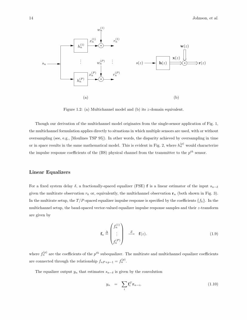
Figure 1.2: (a) Multichannel model and (b) its z-domain equivalent.
Though our derivation of the multichannel model originates from the single-sensor application of Fig. 1,
the multichannel formulation applies directly to situations in which multiple sensors are used, with or without
oversampling (see, e.g., [Moulines TSP 95]). In other words, the disparity achieved by oversampling in time
or in space results in the same mathematical model. This is evident in Fig. 2, where h(p)n would characterize
the impulse response coefficients of the (BS) physical channel from the transmitter to the pth sensor.
Linear Equalizers
For a fixed system delay δ, a fractionally-spaced equalizer (FSE) f is a linear estimator of the input sn−δ
given the multirate observation rk or, equivalently, the multichannel observation rn (both shown in Fig. 3).
In the multirate setup, the T/P -spaced equalizer impulse response is specified by the coefficients {fk}. In the
multichannel setup, the baud-spaced vector-valued equalizer impulse response samples and their z-transform
are given by
fn∆=
f(1)n
...
f(P )n
Z−→ f(z). (1.9)
where f(p)n are the coefficients of the pth subequalizer. The multirate and multichannel equalizer coefficients
are connected through the relationship fnP+p−1 = f(p)n .
The equalizer output yn that estimates sn−δ is given by the convolution
yn =∑
i
fTi rn−i, (1.10)

The Core of FSE-CMA Behavior Theory 15
and can be expressed in the z-domain as
y(z) = fT (z)r(z) = fT (z)h(z)︸ ︷︷ ︸
q(z)
s(z) + fT (z)w(z)︸ ︷︷ ︸
ν(z)
(1.11)
= q(z)s(z) + ν(z). (1.12)
The corresponding multichannel system is depicted in Fig. 3. The transfer function q(z) is often called the
combined channel-equalizer response or the system response. (We will use the latter terminology for the
remainder of the chapter.) Note that, as a polynomial in z, the system response is a baud-rate quantity.
It is important to realize that, once restrictions are placed on the channel and/or equalizer, not all system
responses may be attainable.
Next we consider the case where the channel and equalizer impulse responses are restricted to be finite
in duration. In such a case, the estimate of sn−δ is obtained from the past Lf + 1 multichannel observations
rn, where Lf + 1 denotes the length of the multichannel equalizer. Specifically, we have
yn =
Lf∑
i=0
fTi rn−i = fT r(n), (1.13)
where
f∆=
f0...
fLf
=
f0
...
fP (Lf+1)−1
and r(n)∆=
rn
...
rn−Lf
=
r(n+1)P−1
...
r(n−Lf )P
. (1.14)
The vector-valued received signal in (10.7) can be written as
rn
...
rn−Lf
︸ ︷︷ ︸
r(n)
=
h0 · · · hLh
. . .. . .
h0 · · · hLh
︸ ︷︷ ︸
H
sn
...
sn−Lf−Lh
︸ ︷︷ ︸
s(n)
+
wn
...
wn−Lf
︸ ︷︷ ︸
w(n)
(1.15)
r(n) = Hs(n) + w(n), (1.16)
where H is often referred to as the channel matrix. As evident in (10.14), our construction ensures that the
fractionally-sampled coefficients of the vector quantities r(n), w(n), x(n)∆= Hs(n), and f are well-ordered
with respect to the multirate time-index4. Substituting the received vector expression (10.16) into (10.13),
we obtain the following system output, occurring at the baud rate:
yn = fT Hs(n) + fT w(n) (1.17)
= qT s(n) + νn. (1.18)
The vector q represents the system impulse response (whose coefficients are sampled at the baud rate) and
the quantity νn denotes the filtered channel-noise contribution to the system output.
4Note that the ordering of hn in (10.6) implies h = (h0, h1, . . . , h(Lh+1)P−1)T 6= (hT0 , hT
1 , · · · ,hTLh
)T .

16 Johnson, et al.
+
+
+
+
+
sn
sn
s(z)
hk fk
xk rk
wk
↑ P ↓ P
h(1)n
h(P )n
f(1)n
f(P )n
r(1)n
r(P )n
w(1)n
w(P )n
x(1)n
x(P )n
......
q(z)
w(z)
fT (z)
ν(z)
y(z)
yn
yn
(a)
(b)
(c)
Figure 1.3: Equivalent system models: (a) multirate, (b) multichannel, and (c) their z-domain representation.
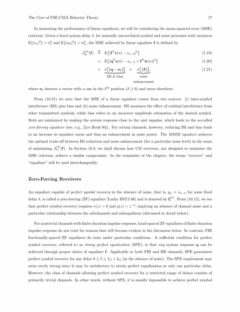
The Core of FSE-CMA Behavior Theory 17
In measuring the performance of linear equalizers, we will be considering the mean-squared error (MSE)
criterion. Given a fixed system delay δ, for mutually uncorrelated symbol and noise processes with variances
E{|sn|2} = σ2s and E{|wk|2} = σ2
w , the MSE achieved by linear equalizer f is defined by
J (δ)m (f)
∆= E
{|fT r(n) − sn−δ|2
}(1.19)
= E{|qT s(n) − sn−δ + fTw(n)|2
}(1.20)
= σ2s‖q− eδ‖2
2︸ ︷︷ ︸
ISI & bias
+ σ2w‖f‖2
2.︸ ︷︷ ︸
noise
enhancement
(1.21)
where eδ denotes a vector with a one in the δth position (δ ≥ 0) and zeros elsewhere.
From (10.21) we note that the MSE of a linear equalizer comes from two sources: (i) inter-symbol
interference (ISI) plus bias and (ii) noise enhancement. ISI measures the effect of residual interference from
other transmitted symbols, while bias refers to an incorrect amplitude estimation of the desired symbol.
Both are minimized by making the system response close to the unit impulse, which leads to the so-called
zero-forcing equalizer (see, e.g., [Lee Book 94]). For certain channels, however, reducing ISI and bias leads
to an increase in equalizer norm and thus an enhancement in noise power. The MMSE equalizer achieves
the optimal trade-off between ISI reduction and noise enhancement (for a particular noise level) in the sense
of minimizing J(δ)m (f). In Section 10.3, we shall discuss how CM receivers, not designed to minimize the
MSE criterion, achieve a similar compromise. In the remainder of the chapter, the terms “receiver” and
“equalizer” will be used interchangeably.
Zero-Forcing Receivers
An equalizer capable of perfect symbol recovery in the absence of noise, that is, yn = sn−δ for some fixed
delay δ, is called a zero-forcing (ZF) equalizer [Lucky BSTJ 66] and is denoted by f(δ)z . From (10.12), we see
that perfect symbol recovery requires ν(z) = 0 and q(z) = z−δ, implying an absence of channel noise and a
particular relationship between the subchannels and subequalizers (discussed in detail below).
For nontrivial channels with finite-duration impulse response, baud-spaced ZF equalizers of finite-duration
impulse response do not exist for reasons that will become evident in the discussion below. In contrast, FIR
fractionally-spaced ZF equalizers do exist under particular conditions. A sufficient condition for perfect
symbol recovery, referred to as strong perfect equalization (SPE), is that any system response q can be
achieved through proper choice of equalizer f . Applicable to both FIR and IIR channels, SPE guarantees
perfect symbol recovery for any delay 0 ≤ δ ≤ Lf + Lh (in the absence of noise). The SPE requirement may
seem overly strong since it may be satisfactory to attain perfect equalization at only one particular delay.
However, the class of channels allowing perfect symbol recovery for a restricted range of delays consists of
primarily trivial channels. In other words, without SPE, it is usually impossible to achieve perfect symbol
18 Johnson, et al.
recovery for a fixed delay.
A necessary and sufficient condition for SPE is that the channel matrix H is full column rank, which
has implications for the subchannel and subequalizer polynomials h(p)(z) = Z{h(p)n } and f (p)(z) = Z{f (p)
n },respectively. A fundamental requirement for SPE is that the subchannel polynomials must not all share a
common zero, that is, {h(p)(z)} must be coprime5. This is often described by the condition: ∀z, h(z) 6= 0.
It can be shown [Tong TIT 95] that when the {h(p)(z)} are coprime, there exists a minimum equalizer length
for which the channel matrix H has full column rank, thus ensuring SPE. Specifically, Lf ≥ Lh − 1 is a
sufficient equalizer length condition when the subchannels are coprime.
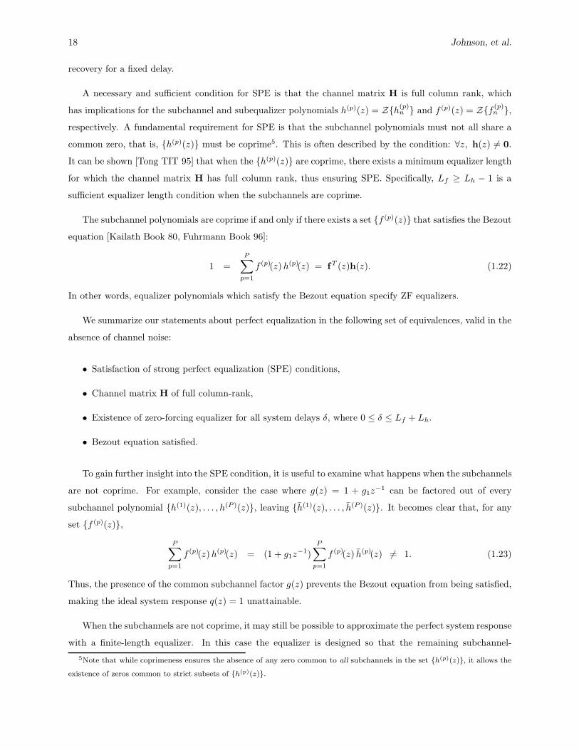
The subchannel polynomials are coprime if and only if there exists a set {f (p)(z)} that satisfies the Bezout
equation [Kailath Book 80, Fuhrmann Book 96]:
1 =P∑
p=1
f (p)(z)h(p)(z) = fT (z)h(z). (1.22)
In other words, equalizer polynomials which satisfy the Bezout equation specify ZF equalizers.
We summarize our statements about perfect equalization in the following set of equivalences, valid in the
absence of channel noise:
• Satisfaction of strong perfect equalization (SPE) conditions,
• Channel matrix H of full column-rank,
• Existence of zero-forcing equalizer for all system delays δ, where 0 ≤ δ ≤ Lf + Lh.
• Bezout equation satisfied.
To gain further insight into the SPE condition, it is useful to examine what happens when the subchannels
are not coprime. For example, consider the case where g(z) = 1 + g1z−1 can be factored out of every
subchannel polynomial {h(1)(z), . . . , h(P )(z)}, leaving {h(1)(z), . . . , h(P )(z)}. It becomes clear that, for any
set {f (p)(z)},
P∑
p=1
f (p)(z)h(p)(z) = (1 + g1z−1)
P∑
p=1
f (p)(z) h(p)(z) 6= 1. (1.23)
Thus, the presence of the common subchannel factor g(z) prevents the Bezout equation from being satisfied,
making the ideal system response q(z) = 1 unattainable.
When the subchannels are not coprime, it may still be possible to approximate the perfect system response
with a finite-length equalizer. In this case the equalizer is designed so that the remaining subchannel-
5Note that while coprimeness ensures the absence of any zero common to all subchannels in the set {h(p)(z)}, it allows the
existence of zeros common to strict subsets of {h(p)(z)}.

The Core of FSE-CMA Behavior Theory 19
subequalizer combinations approximate a delayed inverse of g(z), that is,
P∑
p=1
f (p)(z) h(p)(z) ≈ g−1(z) z−δ (1.24)
In general, the approximation improves as the equalizer length is increased, though performance will depend
on the choice of system delay δ : 0 ≤ δ ≤ Lf + Lh. The implication here is that long enough equalizers can
well approximate zero-forcing equalizers even in the presence of common subchannel roots (as long as the
common roots do not lie on the z-plane’s unit circle).
We can also examine the effect of common zero(s) in the time domain via a decomposition of the channel
matrix H. If an order Lg polynomial g(z) can be factored out of every subchannel, then it can be factored
out of each row of the vector polynomial h(z) leaving h(z) (of order Lh − Lg). We exploit this in the
decomposition H = HG, where
H =
h0 · · · hLh−Lg
. . .. . .
h0 · · · hLh−Lg
and G =
g0 · · · gLg
. . .. . .
g0 · · · gLg
. (1.25)
The matrix H is full column rank with dimension P (Lf +1) × (Lf +Lh−Lg+1), while G is full row rank
with dimension (Lf +Lh−Lg+1) × (Lf +Lh+1). Since the rank of H cannot exceed (Lf +Lh−Lg+1) and
H has (Lf +Lh+1) columns, the choice of Lg > 0 prevents H from achieving full column rank.
Finally, it is worth mentioning that the presence of a common subchannel root is associated with P roots
of the FS channel polynomial (i.e., h0 + h1z−1 + · · · + hP (Lh+1)z
−P (Lh+1)) lying equally spaced on a circle
in the complex plane [Tong TIT 95]. In the case of P = 2, this implies that common subchannel roots are
equivalent to FS channel roots reflected across the origin.
Wiener Receivers
For a fixed system delay δ, the Wiener receiver f(δ)m estimates the source symbol sn−δ by minimizing the
MSE cost
J (δ)m (f) = E
{|fT r(n) − sn−δ|2
}, (1.26)
f (δ)m
∆= arg min
fJ (δ)
m (f). (1.27)
For notational simplicity, the remainder of Section 10.2 assumes that the input sn is a zero-mean, unit-
variance (σ2s = E{|sn|2} = 1), uncorrelated random process. Furthermore, we assume that the channel noise
{wk} is an uncorrelated process with variance σ2w that is uncorrelated with the source.
The theory of MMSE estimation is well established and widely accessible (see, e.g., [Haykin Book 96]).
Since we will find it convenient to refer to the geometrical aspects of MMSE estimation, especially later in
20 Johnson, et al.
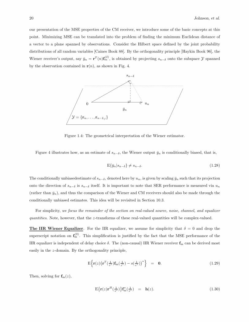
our presentation of the MSE properties of the CM receiver, we introduce some of the basic concepts at this
point. Minimizing MSE can be translated into the problem of finding the minimum Euclidean distance of
a vector to a plane spanned by observations. Consider the Hilbert space defined by the joint probability
distributions of all random variables [Caines Book 88]. By the orthogonality principle [Haykin Book 96], the
Wiener receiver’s output, say yn = rT (n)f(δ)m , is obtained by projecting sn−δ onto the subspace Y spanned
by the observation contained in r(n), as shown in Fig. 4.
0
Y = {rn, . . . , rn−Lf}
sn−δ
yn
un
Figure 1.4: The geometrical interpretation of the Wiener estimator.
Figure 4 illustrates how, as an estimate of sn−δ, the Wiener output yn is conditionally biased, that is,
E{yn|sn−δ} 6= sn−δ. (1.28)
The conditionally unbiasedestimate of sn−δ, denoted here by un, is given by scaling yn such that its projection
onto the direction of sn−δ is sn−δ itself. It is important to note that SER performance is measured via un
(rather than yn), and thus the comparison of the Wiener and CM receivers should also be made through the
conditionally unbiased estimates. This idea will be revisited in Section 10.3.
For simplicity, we focus the remainder of the section on real-valued source, noise, channel, and equalizer
quantities. Note, however, that the z-transforms of these real-valued quantities will be complex-valued.
The IIR Wiener Equalizer. For the IIR equalizer, we assume for simplicity that δ = 0 and drop the
superscript notation on f(0)m . This simplification is justified by the fact that the MSE performance of the
IIR equalizer is independent of delay choice δ. The (non-causal) IIR Wiener receiver fm can be derived most
easily in the z-domain. By the orthogonality principle,
E{
r(z)(rT ( 1
z∗)fm( 1
z∗) − s( 1
z∗))∗}
= 0. (1.29)
Then, solving for fm(z),
E{r(z)rH( 1
z∗)}f∗m( 1
z∗) = h(z). (1.30)
The Core of FSE-CMA Behavior Theory 21
Finally, using r(z) = h(z)s(z) + w(z) and the Matrix Inversion Lemma6 [Kailath Book 80],
fm(z) =1
hT (z)h∗( 1z∗
) + σ2w
h∗( 1z∗
), (1.31)
where σ2w = E{|wk|2} is the noise power. By setting z = ejω , we obtain the frequency response of the Wiener
equalizer:
fm(ejω) =1
‖h(ejω)‖2 + σ2w
h∗(ejω). (1.32)
The denominator term ‖h(ejω)‖2 =∑P
p=1 |h(p)(ejω)|2 is sometimes called the folded channel spectrum
[Lee Book 94, p. 228]. Recall that h(p)(ejω) is the frequency response of the pth subchannel.
System Response. The combined channel-equalizer response qm(z) resulting from IIR Wiener equalization is
qm(z) = fTm(z)h(z) =
hH( 1z∗
)h(z)
hH( 1z∗
)h(z) + σ2w
, (1.33)
or in the frequency domain
qm(ejω) =‖h(ejω)‖2
‖h(ejω)‖2 + σ2w
. (1.34)
As σ2w → 0, qm(z)→ 1 as long as the subchannels have no common roots on the unit circle (i.e., ∀ω, ∃ p,`
s.t. h(p)(ejω) 6= h(`)(ejω)). In this case, the folded spectrum has no nulls and perfect symbol recovery is
achieved.
MMSE of IIR Wiener Receiver . Using (10.11), the estimation error of the IIR Wiener receiver is given by
e(z) = s(z) − y(z) =(1 − fT
m(z)h(z))s(z) − fT
m(z)w(z). (1.35)
Then, with the assumption that σ2s = 1, the power spectrum of the error sequence of the Wiener filter has
the form
Se(ω) = |1 − fTm(ejω)h(ejω)|2 + σ2
w‖fm(ejω)‖2 (1.36)
=σ2
w
‖h(ejω)‖2 + σ2w
. (1.37)
The MSE Em of the Wiener filter is then given by
Em =1
2π
∫ π
−π
σ2w
‖h(ejω)‖2 + σ2w
dω. (1.38)
6The matrix inversion lemma is commonly written as A−1 = (B−1 +CD−1CH)−1 = B−BC(D+CHBC)−1CHB where
A and B are positive definite M × M matrices, D is a positive definite N × N matrix, and C is an M × N matrix. In
deriving (10.31) we use the inversion lemma to find A−1, where A = E˘
r(z)rH( 1z∗
)¯
, by choosing B = 1/σ2w , C = h(z), and
D = 1/σ2s = 1.
22 Johnson, et al.
The FIR Wiener Equalizer. When the vector equalizer polynomial f(δ)m (z) is of finite order, it is con-
venient to derive the Wiener equalizer in the time-domain. From Fig. 4, the Wiener receiver satisfies the
orthogonality principle:(sn−δ − yn
)⊥ r(n), or more specifically,
E{r(n)(sn−δ − yn)
}= 0. (1.39)
Equation (10.39) leads, via (10.13), to the Wiener-Hopf equation whose solution is the Wiener receiver
[Haykin Book 96]:
Rr,rf(δ)m = d(δ)
r,s ⇒ f (δ)m = R†
r,rd(δ)r,s . (1.40)
Here Rr,r∆= E{r(n)rT (n)}, d
(δ)r,s
∆= E{r(n) sn−δ}, and (·)† denotes the Moore-Penrose pseudo-inverse
[Strang Book 88]. In the case of mutually uncorrelated input and noise processes and σ2s = 1, Rr,r =
HHT + σ2wI and d
(δ)r,s = Heδ. This yields the following expression for the FIR Wiener equalizer:
f (δ)m = (HHT + σ2
wI)†Heδ. (1.41)
With the help of the singular value decomposition (SVD) [Strang Book 88], we can obtain an interpre-
tation of the FIR Wiener receiver that is analogous to (10.33). Let H have the following SVD:
H = UΣVT , with Σ = diag{ς0, . . . , ςLf+Lh}, (1.42)
where Σ has the same dimensions as H (which may not be square) and has the singular values {ςi} on its
first diagonal. We then have
f (δ)m = U(ΣΣT + σ2
wI)†ΣVT eδ. (1.43)
The above formula resembles the frequency-domain solution given in (10.31)-(10.32). In fact, (10.43) can be
rewritten as
f (δ)m = Udiag
{
ς0ς20 + σ2
w
, . . . ,ςLf+Lh
ς2Lf+Lh
+ σ2w
}
VT eδ. (1.44)
Note that the terms involving the singular values {ςi} in (10.44) have a form reminiscent of the frequency
response in (10.32).
System Response. The Wiener system response is given by
q(δ)m = HT f (δ)
m = HT (HHT + σ2wI)†Heδ. (1.45)
To obtain a form similar to that of the IIR case, we use the SVD expressions (10.42) and (10.43) to obtain
q(δ)m = VΣT (ΣΣT + σ2
wI)†ΣVT eδ, (1.46)

The Core of FSE-CMA Behavior Theory 23
where the singular values of the channel matrix play the role of magnitude spectrum of the channel in the
IIR case. When H has column dimension less than or equal to its row dimension7 column rank H we have
q(δ)m = V diag
{
ς20
ς20 + σ2
w
, · · · ,ς2Lf+Lh
ς2Lf+Lh
+ σ2w
}
VTeδ. (1.47)
Note the similarity between (10.33) and (10.47). Again, as σ2w → 0, q
(δ)m → eδ, and perfect symbol recovery
is achieved. In this case, the Wiener and ZF equalizers are identical (f(δ)m = f
(δ)z ). We note in advance
that, for full column rank H (i.e., ςi > 0) and σ2w = 0, CM receivers also achieve perfect symbol recovery
up to a fixed phase ambiguity. On the other hand, by increasing σ2w/σ2
s → ∞, q(δ)m approaches the origin.
Interestingly, this property is not shared by the CM receivers, as we shall describe in Section 10.3.
MMSE of FIR Wiener Receiver . For a given system delay δ and equalizer length P (Lf + 1), the MMSE
E(δ)m is defined as J
(δ)m (f
(δ)m ). A simplified expression may be obtained by substituting the Wiener expression
(10.41) into
E(δ)m = ‖HT f (δ)
m − eδ‖22 + σ2
w‖f (δ)m ‖2
2, (1.48)
or can be obtained by first applying the orthogonality principle (10.39) to the MSE definition (10.26) and
then substituting the expression (10.41) as follows:
E(δ)m = E
{|rT (n)f (δ)
m − sn−δ|2}
= E{−sn−δ
(rT (n)f (δ)
m − sn−δ
)}
= 1 − eTδ HT (HHT + σ2
wI)†Heδ. (1.49)
Effects of various parameters on the MMSE can be analyzed using the SVD. Substituting (10.42) into (10.49),
we get
E(δ)m = 1 −
Lf+Lh∑
i=0
ς2i
ς2i + σ2
w
|vδ,i|2 =
Lf+Lh∑
i=0
σ2w
ς2i + σ2
w
|vδ,i|2, (1.50)
where vδ,i is the (δ, i)th entry of V, that is, the δth entry of the ith right singular vector of H.
From (10.50) we see that E(δ)m depends on four factors: (i) the noise power, (ii) the subequalizer order
Lf , (iii) the singular values and singular vectors of the channel matrix H, and (iv) the system delay δ.
• Effects of Noise: As σ2w → 0, E(δ)
m decreases, but not necessarily to zero. The only case in which E(δ)m
approaches zero (for all δ) is when ςi > 0, that is, H has full column rank. For non-zero σ2w, (10.48)
indicates that the MMSE equalizer achieves a compromise between noise gain (i.e., ‖f (δ)m ‖2) and ISI
(i.e., ‖q(δ)m − eδ‖2).
7If H has more columns than rows, that is, the equalizer is “undermodelled” with respect to the channel, then q(δ)m =
V diag
(
ς20ς20+σ2
w
, · · · ,ς2Lf +Lh
ς2Lf +Lh
+σ2w
, 0, . . . , 0
)
VT eδ.

24 Johnson, et al.
• Subequalizer Order Lf : E(δ)m is a non-increasing function of Lf . Using the Toeplitz distribution theorem
[Gray TIT 72], it can be shown that the FIR MMSE (10.50) approaches the IIR MMSE (10.38) as
Lf → ∞, which is intuitively satisfying. In practice, the selection of Lf leads to a tradeoff between
desired performance and implementation complexity.
• Effects of Channel: For FIR equalizers, (10.50) suggests a relatively complex relationship between
MMSE and the singular values and right singular vectors of the channel matrix. In the case of IIR
equalizers, there exists a much simpler relationship between channel properties and MMSE perfor-
mance. Specifically, (10.38) indicates that common subchannel roots near the unit circle cause an
increase in MMSE. Though the relationship between MMSE and subchannel roots is less obvious in
the case of an FIR equalizer, it has been shown that increasing the proximity of subchannel roots
decreases the product of the singular values (see [Fijalkow SPWSSAP 96] and [Casas DSP 97]). Fur-
thermore, the effects of near-common subchannel roots are more severe when noise power is large.
Unfortunately, however, a direct link between subchannel root locations and FIR MMSE has yet to be
found.
• System Delay δ: For FIR Wiener receivers, selection of δ may affect MMSE significantly. This can
be seen in (10.49), where the δth diagonal element of the matrix quantity HT (HHT + σ2wI)†H is
extracted by the eδ pair. Figure 22 in Section 10.4 shows an example of E(δ)m for various equalizer
lengths. Typically, a low-MSE “trough” exists for system delays in the vicinity of the channel’s center
of gravity, and system delays outside of this trough exhibit markedly higher MMSE. This can be
contrasted to the performance of the IIR Wiener receiver which is invariant to delay choice. We note
in advance that system delay is not a direct design parameter with CMA-adapted FIR equalizers (as
discussed in Section 10.4).
The LMS Algorithm
The LMS algorithm [Widrow Book 85] is one of the most widely used stochastic gradient descent (SGD)
algorithms for adaptively minimizing MSE. In terms of the instantaneous squared error
J (δ)m (n)
∆=
1
2|yn − sn−δ|2, (1.51)
the real-valued LMS parameter-vector update equation is
f(n + 1) = f(n) − µ∇f J(δ)m (n) (1.52)
= f(n) − µr(n)(yn − sn−δ
). (1.53)
where ∇f denotes the gradient with respect to the equalizer coefficient vector and µ is a (small) positive
step-size. In practice, a training sequence sent by the transmitter and known a priori by receiver is used to
supply the sn−δ term in (10.53).
The Core of FSE-CMA Behavior Theory 25
Standard analysis of LMS considers the transient and steady-state properties of the algorithm separately.
Detailed expositions on LMS can be found in, e.g., [Haykin Book 96], [Widrow Book 85], [Gitlin Book 92],
and [Macchi Book 95]. We shall review the basic behavior of the LMS algorithm (e.g., excess MSE and
convergence rate) in the equalization context for later comparison with the CM-minimizing algorithm CMA.
Many similarities can be found between LMS and CMA because both attempt to minimize their respective
costs (J(δ)m and Jcm) using a stochastic gradient descent technique.
Transient behavior. The principal item of interest in the transient behavior of LMS is convergence rate.
Because the MSE cost J(δ)m is quadratic, the Hessian is constant throughout the parameter space and thus
convergence rate analysis is straightforward. (The Hessian matrix, defined as ∇f∇fT J(δ)m , determines the
curvature of the cost surface.) Below we derive bounds on the convergence rate of an FIR equalizer.
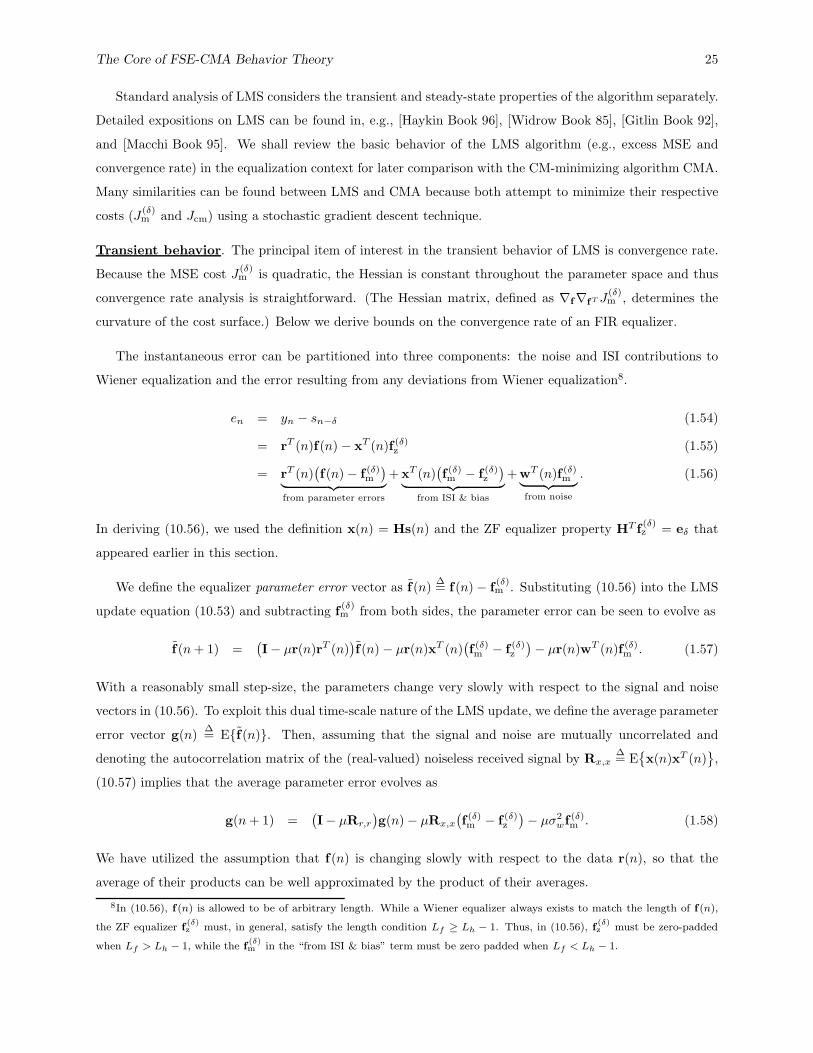
The instantaneous error can be partitioned into three components: the noise and ISI contributions to
Wiener equalization and the error resulting from any deviations from Wiener equalization8.
en = yn − sn−δ (1.54)
= rT (n)f(n) − xT (n)f (δ)z (1.55)
= rT (n)(f(n) − f (δ)
m
)
︸ ︷︷ ︸
from parameter errors
+xT (n)(f (δ)m − f (δ)
z
)
︸ ︷︷ ︸
from ISI & bias
+wT (n)f (δ)m
︸ ︷︷ ︸
from noise
. (1.56)
In deriving (10.56), we used the definition x(n) = Hs(n) and the ZF equalizer property HT f(δ)z = eδ that
appeared earlier in this section.
We define the equalizer parameter error vector as f(n)∆= f(n) − f
(δ)m . Substituting (10.56) into the LMS
update equation (10.53) and subtracting f(δ)m from both sides, the parameter error can be seen to evolve as
f (n + 1) =(I− µr(n)rT (n)
)f(n) − µr(n)xT (n)
(f (δ)m − f (δ)
z
)− µr(n)wT (n)f (δ)
m . (1.57)
With a reasonably small step-size, the parameters change very slowly with respect to the signal and noise
vectors in (10.56). To exploit this dual time-scale nature of the LMS update, we define the average parameter
error vector g(n)∆= E{f(n)}. Then, assuming that the signal and noise are mutually uncorrelated and
denoting the autocorrelation matrix of the (real-valued) noiseless received signal by Rx,x∆= E
{x(n)xT (n)
},
(10.57) implies that the average parameter error evolves as
g(n + 1) =(I− µRr,r
)g(n) − µRx,x
(f (δ)m − f (δ)
z
)− µσ2
wf (δ)m . (1.58)
We have utilized the assumption that f(n) is changing slowly with respect to the data r(n), so that the
average of their products can be well approximated by the product of their averages.
8In (10.56), f(n) is allowed to be of arbitrary length. While a Wiener equalizer always exists to match the length of f(n),
the ZF equalizer f(δ)z must, in general, satisfy the length condition Lf ≥ Lh − 1. Thus, in (10.56), f
(δ)z must be zero-padded
when Lf > Lh − 1, while the f(δ)m in the “from ISI & bias” term must be zero padded when Lf < Lh − 1.
26 Johnson, et al.
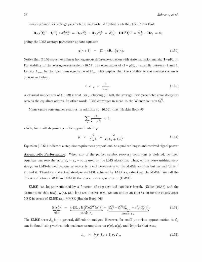
Our expression for average parameter error can be simplified with the observation that
Rx,x
(f (δ)m − f (δ)
z
)+ σ2
wf (δ)m = Rr,rf
(δ)m − Rx,xf
(δ)z = d(δ)
r,s − HHT f (δ)z = d(δ)
r,s − Heδ = 0,
giving the LMS average parameter update equation
g(n + 1) =(I − µRr,r
)g(n). (1.59)
Notice that (10.59) specifies a linear homogeneous difference equation with state transition matrix (I−µRr,r).
For stability of the average-error-system (10.59), the eigenvalues of (I − µRr,r) must lie between -1 and 1.
Letting λmax be the maximum eigenvalue of Rr,r, this implies that the stability of the average system is
guaranteed when
0 < µ <2
λmax. (1.60)
A classical implication of (10.59) is that, for µ obeying (10.60), the average LMS parameter error decays to
zero as the equalizer adapts. In other words, LMS converges in mean to the Wiener solution f(δ)m .
Mean-square convergence requires, in addition to (10.60), that [Haykin Book 96]
∑
i
µλi
2 − µλi< 1,
which, for small step-sizes, can be approximated by
µ <2
∑
i λi=
2
P (Lf + 1)σ2r
. (1.61)
Equation (10.61) indicates a step-size requirement proportional to equalizer length and received signal power.
Asymptotic Performance. When any of the perfect symbol recovery conditions is violated, no fixed
equalizer can zero the error en = yn − sn−δ used by the LMS algorithm. Thus, with a non-vanishing step-
size µ, an LMS-derived parameter vector f(n) will never settle to the MMSE solution but instead “jitter”
around it. Therefore, the actual steady-state MSE achieved by LMS is greater than the MMSE. We call the
difference between MSE and MMSE the excess mean square error (EMSE).
EMSE can be approximated by a function of step-size and equalizer length. Using (10.56) and the
assumptions that x(n), w(n), and f(n) are uncorrelated, we can obtain an expression for the steady-state
MSE in terms of EMSE and MMSE [Haykin Book 96]:
E{e2n}
︸ ︷︷ ︸
MSE
= tr(Rr,r E
{f(n)fT (n)
})
︸ ︷︷ ︸
EMSE, Eχ
+ ‖f (δ)m − f (δ)
z ‖2Rx,x
+ σ2w‖f (δ)
m ‖22
︸ ︷︷ ︸
MMSE, Em
. (1.62)
The EMSE term Eχ is, in general, difficult to analyze. However, for small µ, a close approximation to Eχ
can be found using various independence assumptions on r(n), s(n), and f(n). In that case,
Eχ ≈ µ
2P (Lf + 1)σ2
r Em, (1.63)
The Core of FSE-CMA Behavior Theory 27
where σ2r
∆= E{|rk|2} is the received signal power [Haykin Book 96]. Note that EMSE is proportional to the
product of step-size, equalizer length, received signal power, and MMSE. Recall that P (Lf + 1) represents
the total number of adapted equalizer coefficients.
LMS Design Implications. The form of the EMSE expression (10.63) has a number of design implications
for LMS-based adaptive equalization.
For one, there is the step-size tradeoff: a large step-size gives fast convergence to an equalizer with large
EMSE while a small step-size gives slow convergence to an equalizer with small EMSE. This suggests making
µ as small as possible within allowed limits on convergence time. When the channel impulse response is time-
varying, however, the situation becomes more complicated: step-sizes that are too small may not be able
to adequately track the channel variations, resulting in what is known as tracking lag [Widrow PROC 76].
Tracking lag prevents the equalizer from remaining in close vicinity to the time-varying f(δ)m which ultimately
increases MSE. Increasing the step-size may reduce tracking lag but may increase Eχ via (10.63). Thus, even
in time-varying situations, step-sizes that are too large ultimately increase steady-state MSE via (10.62).
Hence, the best step-size is a compromise between these situations.
There is a similar tradeoff with equalizer length P (Lf +1). Equalizers that are too short result in a high
MMSE, which prohibits a low steady-state MSE via (10.62). On the other hand, very long equalizers may
result in a large EMSE via (10.63), also preventing good steady-state MSE performance. Thus, the optimal
equalizer length lies somewhere in between.
The analysis of Section 10.3 will demonstrate that CMA shares many of the same behavior features of
LMS. Hence, many of the CMA design guidelines in Section 10.4 can be related back to the LMS design
guidelines discussed in this section.

28 Johnson, et al.
1.3 The CM Criterion and CMA
This section focuses on the properties of the CM criterion and the behavior of the Constant Modulus Algo-
rithm (CMA). What will be a recurring theme can be summarized by Godard’s conjecture, an observation
made by Godard in his seminal paper on blind adaptive (baud-spaced) equalization. In [Godard TCOM 80],
Godard observed that the MSE performance of CMA is close to that of the MMSE-optimal (Wiener) equal-
izer:
“It should also be noted that the equalizer coefficients minimizing the dispersion functions closely
approximate those which minimize the mean-squared error.” —Godard (1980).
Treichler and Agee made a similar claim in their independent development of the CM criterion
[Treichler TASSP 83]. Throughout this section, we shall provide evidence supporting Godard’s conjecture.
This section is organized as follows. We first introduce the CM criterion and present what are known as
the Perfect Blind Equalization (PBE) conditions. Simple illustrated examples are provided to understand the
effects of violating these conditions. Next, properties of the local and global minima of the CM cost function
(referred to as CM receivers) are discussed and compared to that of the well-known Wiener and zero-forcing
receivers discussed in Section 10.2. This is followed by summaries of important analytical work concerning
the robustness of CM receivers to the presence of noise and channel undermodelling. Both perturbation-based
approximations and bounds from a geometrical approach are used to predict CM performance in a practical
setting. The section concludes by summarizing the transient and asymptotic behavior of CMA, a stochastic
gradient descent (SGD) algorithm popularly employed to adapt blind equalizers, which minimizes the CM
criterion. Various comparisons are drawn between CMA and the well-known LMS algorithm (discussed in
Section 10.2).
Properties of the CM Criterion
Functional Form. Blind equalization can be considered as the estimation of (unknown) source symbols
{sn} from the receiver input sequence {rn}, or equivalently {r(n)}. In our formulation of the problem, the
linear filter f generates the symbol estimate yn = fT r(n), and we desire that yn ≈ sn−δ for some fixed integer
delay δ.
In motivating the CM criterion, we first consider the family of Bussgang techniques used in blind equal-
ization [Bellini (Haykin) 94]. Some intuition behind these Bussgang techniques comes from a consideration
of trained and decision-directed LMS-based equalizer adaptation, described by the update equation
f(n + 1) = f(n) − µ r∗(n) en. (1.64)
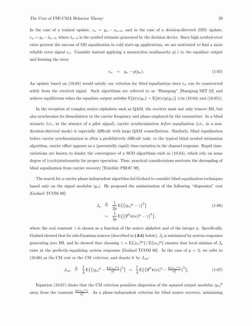
The Core of FSE-CMA Behavior Theory 29
In the case of a trained update, en = yn − sn−δ, and in the case of a decision-directed (DD) update,
en = yn− sn−δ, where sn−δ is the symbol estimate generated by the decision device. Since high symbol-error
rates prevent the success of DD equalization in cold start-up applications, we are motivated to find a more
reliable error signal en. Consider instead applying a memoryless nonlinearity g(·) to the equalizer output
and forming the error
en = yn − g(yn). (1.65)
An update based on (10.65) would satisfy our criterion for blind equalization since en can be constructed
solely from the received signal. Such algorithms are referred to as “Bussgang” [Bussgang MIT 52] and
achieve equilibrium when the equalizer output satisfies E{r(n)yn} = E{r(n)g(yn)} (via (10.64) and (10.65)).
In the reception of complex source alphabets such as QAM, the receiver must not only remove ISI, but
also synchronize its demodulator to the carrier frequency and phase employed by the transmitter. In a blind
scenario (i.e., in the absence of a pilot signal), carrier synchronization before equalization (i.e., in a non-
decision-directed mode) is especially difficult with large QAM constellations. Similarly, blind equalization
before carrier synchronization is often a prohibitively difficult task: to the typical blind symbol estimation
algorithm, carrier offset appears as a (potentially rapid) time-variation in the channel response. Rapid time-
variations are known to hinder the convergence of a SGD algorithms such as (10.64), which rely on some
degree of (cyclo)stationarity for proper operation. Thus, practical considerations motivate the decoupling of
blind equalization from carrier recovery [Treichler PROC 98].
The search for a carrier-phase independent algorithm led Godard to consider blind equalization techniques
based only on the signal modulus |yn|. He proposed the minimization of the following “dispersion” cost
[Godard TCOM 80]:
Jp∆=
1
2pE{(
|yn|p − γ)2}
(1.66)
=1
2pE{(
|fT r(n)|p − γ)2}
,
where the real constant γ is chosen as a function of the source alphabet and of the integer p. Specifically,
Godard showed that for sub-Gaussian sources (described in (A4) below), Jp is minimized by system responses
generating zero ISI, and he showed that choosing γ = E{|sn|2p}/ E{|sn|p} ensures that local minima of Jp
exist at the perfectly-equalizing system responses [Godard TCOM 80]. In the case of p = 2, we refer to
(10.66) as the CM cost or the CM criterion, and denote it by Jcm:
Jcm∆=
1
4E{(
|yn|2 − E{|sn|4}σ2
s
)2}=
1
4E{(
|fT r(n)|2 − E{|sn|4}σ2
s
)2}, (1.67)
Equation (10.67) shows that the CM criterion penalizes dispersion of the squared output modulus |yn|2
away from the constant E{|sn|4}σ2
s. As a phase-independent criterion for blind source recovery, minimizing
30 Johnson, et al.
dispersion seems intuitively satisfying for CM sources9. Remarkably, the CM criterion works almost as well
with non-CM sources. We note that the CM idea was independently proposed for constant-modulus source
sequences (i.e., ∃ ρ ∈ R s.t. ∀n, |sn| = ρ) by Treichler and Agee in [Treichler TASSP 83].
It is important to note that Godard’s blind equalization algorithm belongs to the Bussgang class. In fact,
it can be shown to approximate the conditional-mean estimator of |sn|2 given |yn|2 [Bellini (Haykin) 94], a
valid estimator in the absence of carrier phase information (or equivalently, when all rotations of the source
constellation are assumed equally likely).
Having introduced the CM criterion as a phase-independent means of blind equalization (thus intended
for complex-valued signals) it may seem strange that in the sequel we restrict our analysis to the case of
real-valued quantities. We justify our position by claiming that nearly all of the intuition concerning the
behavior of the CM criterion can be gained from the study of its real-valued incarnation with the benefit of
a simplified presentation. We will attempt to note any situations in which complex-valued quantities lead to
meaningful conceptual differences. With this in mind, we present a useful expansion of the CM cost in terms
of the equalizer coefficients f for real-valued channels, real-valued i.i.d. noise, and real-valued i.i.d. sources.
(See [Johnson PROC 98] for derivations of this and more general CM cost expressions.)
Jcm =1
4σ4
s(κs − 3)‖HT f‖44 +
3
4σ4
s‖HT f‖42 +
1
4σ4
w(κw − 3)‖f‖44 +
3
4σ4
w‖f‖42
+3
2σ2
sσ2w‖HT f‖2
2 ‖f‖22 −
1
2σ2
sκs(σ2s‖HT f‖2
2 + σ2w‖f‖2
2) +1
4σ4
sκ2s. (1.68)
In the equation above, κs refers to the normalized kurtosis of the source process, defined below in (10.69).
By analogy, κw denotes the kurtosis of the channel noise process {wk}. The quantities σ2s and σ2
w denote
the source and noise variances, respectively. Note that, in the absence of noise, Jcm is a quartic function of
the `4 and `2 norms of the channel-equalizer impulse response HT f . The addition of noise brings a quartic
dependence on the `4 and `2 norms of the equalizer impulse response f .
As we shall see in the following sections, the local and global minimizers of Jcm, that is, the CM receivers
fc, are of key importance. For example, they represent the asymptotic mean-convergence points of the
constant modulus algorithm.
Perfect Blind Equalizability Conditions. The set of conditions under which all minimizers of Jcm ac-
complish perfect symbol recovery are known as the Perfect Blind Equalization (PBE) conditions [Foschini ATT 85,
Fijalkow SPW 94, Li TSP 96a]. They are given below.
(A1) Full column-rank channel matrix H,
(A2) No additive channel noise,
9Sources derived from M -PSK constellations are examples of CM sources, since every symbol in the M -PSK alphabet has
the same magnitude (or “modulus”). M -QAM sources for M > 4 do not have the CM property since alphabet members differ
in magnitude as well as phase. See Fig. 19 for an illustration.

The Core of FSE-CMA Behavior Theory 31
Table 1.7: Summary of Channels Used for Two-Tap FSE Examples.
Name T/2-spaced Impulse Response Classification
ha (−0.0901, 0.6853, 0.7170,−0.0901)T well-behaved11
hb (1.0,−0.5, 0.2, 0.3)T well-behaved
hc (−0.0086, 0.0101, 0.9999,−0.0086)T nearly-common subchannel roots
hd (1.0,−0.5, 0.2, 0.3,−0.2,−0.15)T undermodelled
(A3) Symmetric i.i.d.10 source, circularly symmetric (E{s2n} = 0) in the complex-valued case.
(A4) Sub-Gaussian source: the normalized source kurtosis satisfies κs < κg.
The normalized source kurtosis κs is defined as
κs∆=
E{|sn|4}σ4
s
, (1.69)
where the kurtosis of a real-valued Gaussian random process is κg = 3 and the kurtosis of a proper complex-
valued Gaussian random process is κg = 2. Note that Conditions (A1)-(A2) pertain to the channel-equalizer
pair’s ability to achieve perfect equalization, as discussed in Section 10.2. Conditions (A3) and (A4) pertain
solely to blind equalization based on the CM criterion.
Illustrative Examples of CM Cost Surface Deformations. This section studies changes to the
“shape” of the CM cost surface as a means of understanding the effect of various violations of the PBE
conditions. Restricting our focus to the case of a real-valued two-tap T/2-spaced equalizer permits illustra-
tion of the cost surface as a function of equalizer parameters. We do not intend a rigorous analysis of CM
robustness properties here—that will be the subject of later subsections.
Perfect Blind Equalizability . We first consider a 4-tap channel and 2-tap equalizer, both T/2-spaced (i.e.,
P = 2), satisfying the column rank condition (A1). Associated with this model are the following channel
convolution matrix and equalizer coefficient vector:
H =
h1 h3
h0 h2
, f =
f0
f1
.
A square invertible H ensures unique zero-forcing solutions to ±eδ = HT f for δ ∈ {0, 1}. As discussed in
Section 10.2, the existence of this inverse requires that the even and odd subchannels, h(1)(z) = h0 + h2z−1
and h(2)(z) = h1 + h3z−1, respectively, do not share the same root location. Examples of 4-tap channels
satisfying this non-common-root condition are given by ha and hb in Table 10.7.
10Examination of the derivation in [Johnson PROC 98] reveals that the CM cost expression yielding the global convergence
properties requires only fourth-order statistical independence of the source process.11“Well-behaved” indicates the absence of common or nearly-common subchannel roots.

32 Johnson, et al.
For an i.i.d. source with kurtosis κs = 1 in the absence of channel noise (thus satisfying (A2)-(A4)),
the CM cost is shown in Fig. 5 and 6 as a function of equalizer coefficients. In all upcoming contour plots,
a “∗” indicates a MMSE solution corresponding to an optimal system delay, while a “×” indicates a MMSE
solution corresponding to a sub-optimal system delay. In Fig. 6, however, zero MSE can be achieved at all
system delays and thus all solutions are optimal. It can be seen that when the PBE conditions are satisfied,
the MMSE solutions exactly coincide with the minima of Jcm. Each pair of CM minima symmetric with
respect to the origin corresponds to the same system delay but to two different12 choices of system polarity
(±). Such sign ambiguity is inconsequential when, for example, the symbols have been differentially encoded.
Thus, in Fig. 5, the four minima correspond to the four permutations of system delay (δ = 0, 1) and polarity
(+,−). Note the CM local maximum at the origin.
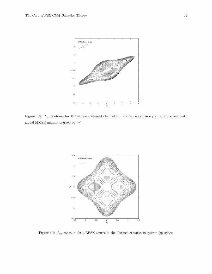
Sometimes it is more convenient to study Jcm as a function of system response q. Note that when H is
square and invertible, as in our current example, there exists a unique mapping between f - and q-spaces:
q = HT f . One appeal of studying Jcm in q-space follows from the normalization and alignment of the Jcm
minima with the coordinate axes. For example, our current ZF system responses occur at q = (±1, 0) and
(0,±1) (see Fig. 7). Such symmetry will be exploited in the section. Under satisfaction of (A1) and (A2),
viewing Jcm from system space has the additional advantage that the CM cost is channel-independent (recall
(10.68) with HT f = q).
−2.5 −2 −1.5 −1 −0.5 0 0.5 1 1.5 2 2.5
−2
−1
0
1
2
0
0.1
0.2
0.3
0.4
0.5
0.6
0.7
0.8
0.9
1
f0
f1
Figure 1.5: Jcm for BPSK, well-behaved channel ha, and no noise, in equalizer (f) space.
Effect of Channel Noise. Violation of (A2) occurs in any communication system where additive channel
noise w(n) is present. We denote the signal-to-noise ratio (SNR) by SNR = 10 log10(σ2s/σ2
w) using the
12In the complex-valued case, each pair of minima would be replaced by a a continuum of minima spanning the full range
(0 − 2π) of allowable system phase.
The Core of FSE-CMA Behavior Theory 33
−4 −3 −2 −1 0 1 2 3 4−4
−3
−2
−1
0
1
2
3
4
f0
f 1
MSE ellipse axes
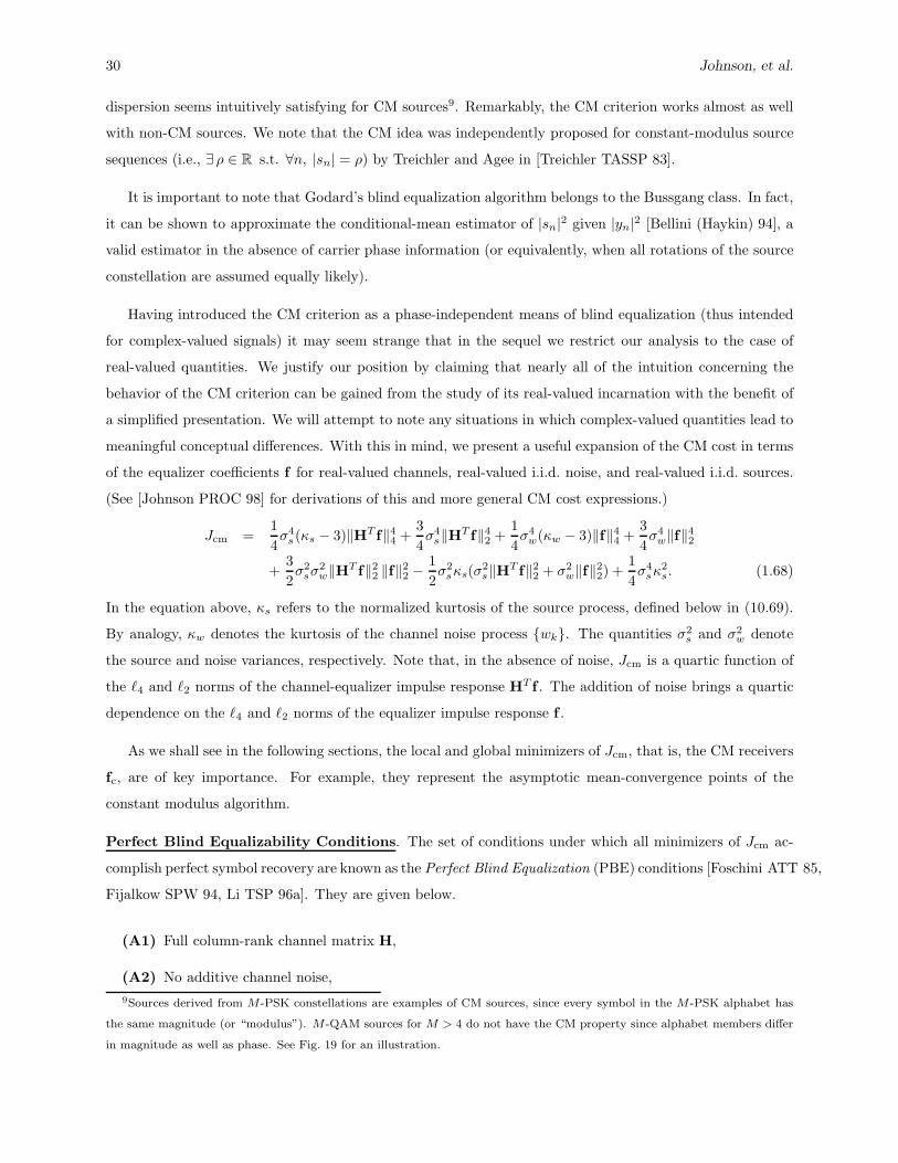
Figure 1.6: Jcm contours for BPSK, well-behaved channel hb, and no noise, in equalizer (f) space, with
global MMSE minima marked by “∗”.
−1.5 −1 −0.5 0 0.5 1 1.5−1.5
−1
−0.5
0
0.5
1
1.5
q0
q 1
MSE ellipse axes
Figure 1.7: Jcm contours for a BPSK source in the absence of noise, in system (q) space.

34 Johnson, et al.
source and noise variances introduced in Section 10.2. The presence of noise causes the shape of the CM
cost surface to change in such a way that the CM minima no longer correspond to the Wiener minima and
such that different CM minima may result in different levels of performance. In other words, we now have
strictly local (versus global) minima. This can be recognized in the contour depths in Fig. 8.
Most importantly, however, Fig. 8 suggests that, even at relatively high noise powers, the CM and MSE
minima roughly correspond. Here we see evidence of Godard’s conjecture. It is interesting to note that the
suboptimal CM minima are further from their neighboring Wiener solutions than the optimal CM minima
are from theirs. The robustness properties of the CM criterion to additive channel noise are the focus of
sections presented in the sequel.
−3 −2 −1 0 1 2 3−3
−2
−1
0
1
2
3
f0
f 1
MSE ellipse axes
Figure 1.8: Jcm contours for channel hb and 20 dB SNR in equalizer (f) space.
Effect of Nearly-Common Subchannel Roots. In Section 10.2 we discussed the effects of (exactly) common
subchannel roots and demonstrated that, in general, they prevent perfect source recovery (hence violating
(A1)). Though nearly-common subchannel roots do not share this problem, they may excite an undesirable
phenomenon known as noise gain, a familiar concept from ZF and MMSE equalization theory. We will see
that a similar phenomenon exists for equalization methods based on minimizing the CM criterion.
One way to understand the mechanics of noise gain is to consider the transformation from the ZF
system responses {q(δ)z } to the respective ZF equalizers {f (δ)
z }. Nearly-common subchannel roots (i.e.,
h3/h1 ≈ h2/h0) result in a transformation matrix (HT )† with large eigenvalues. This has the effect of
mapping certain ZF system responses to ZF equalizers with large norm, as illustrated13 by Fig. 9. These
13Recall that with square invertible H and in the absence of noise the ZF and MMSE equalizers are identical. Thus the ∗’s
in Fig. 9 denote the locations of the ZF equalizers.

The Core of FSE-CMA Behavior Theory 35
large-norm equalizers result in significant noise gain, as indicated by the MSE formula (10.48). In order to
better compromise between ISI cancellation and noise gain, we expect the MMSE optimal equalizers to be
smaller in norm than their ZF counterparts. This is confirmed by the behavior of the Wiener expressions
(10.32) and (10.44) as σ2w is increased. Equation (10.44) also indicates that if H has small singular values
(as would result from nearly-common subchannel roots), f(δ)m will be sensitive to even modest amounts of
noise.
The effects of nearly-common subchannel roots on CM receivers are quite similar. Since nearly-common
roots do not actually violate (A1), the PBE conditions may still be satisfied, as shown by Fig. 9. They
do excite a similar noise gain phenomenon, however, affecting CM receivers quite similarly to their Wiener
counterparts (see Fig. 10). Note again that the better Jcm minima are in close proximity to the better
Wiener solutions, offering evidence for Godard’s conjecture. CM robustness to common subchannels has
been formally addressed in [Fijalkow TSP 97].
−100 −50 0 50 100−1.5
−1
−0.5
0
0.5
1
1.5
f0
f 1
MSE ellipse axes
Figure 1.9: Jcm contours for nearly-common subchannel-roots channel hc and no noise in equalizer (f) space.
Note axis scaling.
Effect of Channel Undermodelling . When the equalizer length is short enough to violate (A1), the equalizer
is, in general, not capable of perfect symbol recovery. This can be demonstrated by leaving our equalizer
length at two taps but extending the hb channel response to (1.0, −0.5, 0.2, 0.3, −0.2, −0.15)T = hd. Now
we have
H =
h1 h3 h5
h0 h2 h4
, f =
f0
f1
.
The dimensions of H indicate that three distinct system delays are now possible, and thus there exist six
Wiener receivers (after allowing ± system polarities). Looking at Fig. 11, however, the number of CM

36 Johnson, et al.
−8 −6 −4 −2 0 2 4 6 8−1.5
−1
−0.5
0
0.5
1
1.5
f0
f 1
MSE ellipse axes
Figure 1.10: Jcm contours for nearly-common subchannel-roots channel hc and 20 dB SNR in equalizer (f)
space. Note axis scaling.
receivers has not increased. It is important to note that the best CM minima are still near the best Wiener
solutions, implying a certain degree of robustness to undermodelling and further evidence for Godard’s
conjecture. These robustness properties are discussed further in an upcoming subsection.
Effect of Source Correlation . PBE condition (A3) specifies a white source sequence. To examine this
condition, Fig. 12 shows the effect of a temporally correlated source on the CM cost surface using noiseless
channel hb and the 4-PAM periodic sequence {sn} = {. . . , 3, 1,−1,−3, . . .}. In comparison to Fig. 6, we can
observe a “twisting” of the cost surface that leads to a significant separation between the CM and Wiener
receivers. More dramatic effects are possible in higher-dimensional systems including a potential increase in
the number of CM local minima [LeBlanc IJACSP 98].
In the complex-valued case, correlation between the real and imaginary components of the source yields
E{s2n} 6= 0, thus violating (A3). [Axford TSP 98] and [Papadias ICASSP 97] discuss the presence of false
CM minima under these conditions.
Effect of Source Kurtosis. Condition (A4) states that the source distribution must be sub-Gaussian (i.e.,
κs < κg) for perfect blind equalizability. This requirement is satisfied by all uniformly-distributed data
constellations, such as M -PAM, M -PSK, and M -QAM. Even so, the value of the (sub-Gaussian) kurtosis
still has an effect on the shape of the CM cost surface. Specifically, as the kurtosis (10.69) increases towards
κg, the CM cost surface rises and all but the radial component of the gradient tends to vanish. Figure 13
shows the surface for a uniformly distributed 32-PAM source, for which κs ≈ 1.8. (Compare to Fig. 5.) Note
that the parameter-space positions of the CM minima are unaltered (as expected, since the PBE conditions
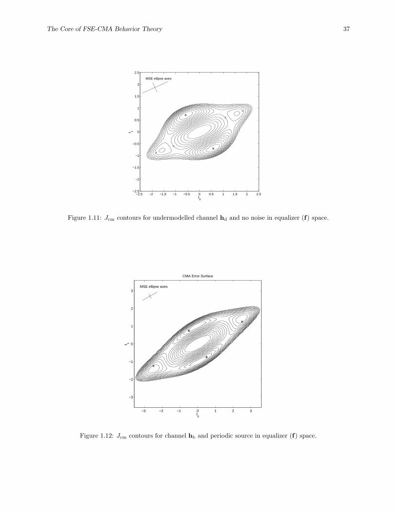
The Core of FSE-CMA Behavior Theory 37
−2.5 −2 −1.5 −1 −0.5 0 0.5 1 1.5 2 2.5−2.5
−2
−1.5
−1
−0.5
0
0.5
1
1.5
2
2.5
f0
f 1
MSE ellipse axes
Figure 1.11: Jcm contours for undermodelled channel hd and no noise in equalizer (f) space.
−3 −2 −1 0 1 2 3
−3
−2
−1
0
1
2
3
f0
f 1
CMA Error Surface
MSE ellipse axes
Figure 1.12: Jcm contours for channel hb and periodic source in equalizer (f) space.

38 Johnson, et al.
are still satisfied). For more information on the effect of source kurtosis on the CM criterion, we refer
interested readers to [LeBlanc IJACSP 98, LeBlanc Thesis 95].
−2.5 −2 −1.5 −1 −0.5 0 0.5 1 1.5 2 2.5
−2
−1
0
1
2
0
0.5
1
1.5
2
2.5
3
3.5
f0
f1
Figure 1.13: Jcm for non-CM source (κs ≈ 1.8) and channel ha in equalizer (f) space.
Properties of CM Stationary Points. Recall that, when the PBE conditions are satisfied, all minima
of the CM cost function are global minima and coincide with the ZF and Wiener receivers. In such a case,
the CM receivers achieve perfect source recovery.
In addition to minima, the CM cost surface exhibits saddle points and one maximum. These extrema,
commonly called stationary points, are described in [Johnson IJACSP 95] for BPSK and a real-valued chan-
nel. With an i.i.d. source and in the absence of channel noise, the CM stationary points can be identified
by having system responses q satisfying particular criteria. Specifically, a stationary point qc satisfies the
zero-gradient condition ∇fJcm = 0, where the equalizer-space gradient ∇fJcm is given below as a function
of q (under (A2) and (A3)):
∇fJcm(q) = σ4sH∆qq. (1.70)
The matrix ∆q is defined (in both the real- and complex-valued cases) as follows:
∆q∆= (κg ‖q‖2
2−κs)I − (κg − κs)Diag(qqH), (1.71)
where κg is the kurtosis of a Gaussian source. The matrix operation Diag(·) retains the diagonal entries of
its argument while replacing the other entries with zeros.
The stability of a CM stationary point (i.e., whether or not it is a local minima) is given by the positive-
semidefiniteness of its equalizer-space Hessian, denoted by HfJcm ≥ 0. The Hessian is given below, for the

The Core of FSE-CMA Behavior Theory 39
case of real-valued quantities14, as a function of q (again, under (A2) and (A3)):
HfJcm = σ4sHΨqH
T . (1.72)
The matrix Ψq is defined as follows:
Ψq∆= (κg ‖q‖2
2−κs)I + 2κgqqT − 3(κg − κs)diag(qqT ). (1.73)
In the case that H is full-column rank, the requirements for q to be a CM minimum reduce to ∆qq = 0 and
Ψq ≥ 0.
In summary, it can be shown (see, e.g., [Fijalkow SPW 94] for the real-valued case) that, under the PBE
conditions,
• all CM minima correspond to ZF system responses, that is, qc = ±eδ for 0 ≥ δ ≥ Lf + Lh;
• the only CM maximum occurs at the origin, that is, q = 0; and
• the CM saddle points are described by system responses composed of coefficients that are either zero
or a fixed magnitude: q = τM
∑M−1i=0 (±ei) where M , the number of nonzero elements in q, obeys
2 ≤ M ≤ Lf +Lh+1 and where τM =√
κs
κg(M−1)+κs. (See Fig. 18.)
Notice that the number and type of stationary points of the CM cost are not affected by the source kurtosis
κs (as long as the source is sub-Gaussian). However, the values of the CM costs at the stationary points, as
well as the locations of the saddle points, remain a function of κs. (This can be verified by substituting the
appropriate q into (10.68).) The relocation of saddle points is important because it affects the shape of the
CM cost surface and, consequently, the performance of SGD minimization algorithms such as CMA. These
issues are discussed further in an upcoming subsection.
Robustness Properties of the CM Criterion
This section summarizes important analytical results pertaining to the robustness of CM-minimizing equal-
izer performance to violations of the PBE conditions. Though we will focus on the robustness to noise and
channel undermodelling, we note that evidence of CM robustness to nearly-common subchannel roots appears
in [Fijalkow TSP 97], and evidence of robustness to correlated sources appears in [LeBlanc IJACSP 98].
The first two subsections below describe performance approximations obtained using perturbation tech-
niques. In general, such techniques measure the effect of local deviations from a reference setting (e.g., a
zero-forcing or MMSE receiver) and are generally valid for small deviations about this reference. Later in
14The complex-valued case requires calculating the partial derivatives of Jcm with respect to the real part and imaginary part
of f separately. For example, the Hessian could be taken with respect to the real-valued vector f = (Re fT , Im fT )T .
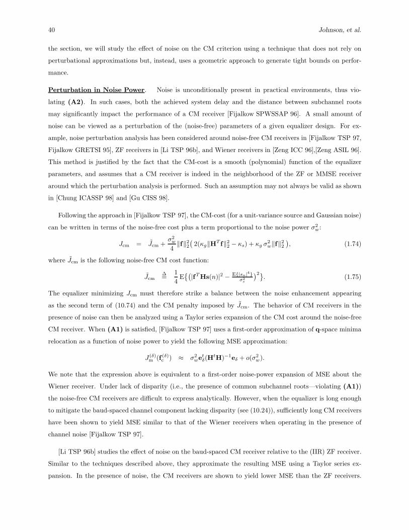
40 Johnson, et al.
the section, we will study the effect of noise on the CM criterion using a technique that does not rely on
perturbational approximations but, instead, uses a geometric approach to generate tight bounds on perfor-
mance.
Perturbation in Noise Power. Noise is unconditionally present in practical environments, thus vio-
lating (A2). In such cases, both the achieved system delay and the distance between subchannel roots
may significantly impact the performance of a CM receiver [Fijalkow SPWSSAP 96]. A small amount of
noise can be viewed as a perturbation of the (noise-free) parameters of a given equalizer design. For ex-
ample, noise perturbation analysis has been considered around noise-free CM receivers in [Fijalkow TSP 97,
Fijalkow GRETSI 95], ZF receivers in [Li TSP 96b], and Wiener receivers in [Zeng ICC 96],[Zeng ASIL 96].
This method is justified by the fact that the CM-cost is a smooth (polynomial) function of the equalizer
parameters, and assumes that a CM receiver is indeed in the neighborhood of the ZF or MMSE receiver
around which the perturbation analysis is performed. Such an assumption may not always be valid as shown
in [Chung ICASSP 98] and [Gu CISS 98].
Following the approach in [Fijalkow TSP 97], the CM-cost (for a unit-variance source and Gaussian noise)
can be written in terms of the noise-free cost plus a term proportional to the noise power σ2w :
Jcm = Jcm +σ2
w
4‖f‖2
2
(2(κg‖HT f‖2
2 − κs) + κg σ2w‖f‖2
2
), (1.74)
where Jcm is the following noise-free CM cost function:
Jcm∆=
1
4E{(
|fTHs(n)|2 − E{|sn|4}σ2
s
)2}. (1.75)
The equalizer minimizing Jcm must therefore strike a balance between the noise enhancement appearing
as the second term of (10.74) and the CM penalty imposed by Jcm. The behavior of CM receivers in the
presence of noise can then be analyzed using a Taylor series expansion of the CM cost around the noise-free
CM receiver. When (A1) is satisfied, [Fijalkow TSP 97] uses a first-order approximation of q-space minima
relocation as a function of noise power to yield the following MSE approximation:
J (δ)m (f (δ)
c ) ≈ σ2wet
δ(HtH)−1eδ + o(σ2
w).
We note that the expression above is equivalent to a first-order noise-power expansion of MSE about the
Wiener receiver. Under lack of disparity (i.e., the presence of common subchannel roots—violating (A1))
the noise-free CM receivers are difficult to express analytically. However, when the equalizer is long enough
to mitigate the baud-spaced channel component lacking disparity (see (10.24)), sufficiently long CM receivers
have been shown to yield MSE similar to that of the Wiener receivers when operating in the presence of
channel noise [Fijalkow TSP 97].
[Li TSP 96b] studies the effect of noise on the baud-spaced CM receiver relative to the (IIR) ZF receiver.
Similar to the techniques described above, they approximate the resulting MSE using a Taylor series ex-
pansion. In the presence of noise, the CM receivers are shown to yield lower MSE than the ZF receivers.

The Core of FSE-CMA Behavior Theory 41
Since the ZF receivers are susceptible to noise gain, this result should not come as a surprise. Recall that
the presence of nearly common subchannel roots can make the performance of ZF receivers very sensitive to
noise.
Leveraging Godard’s conjecture concerning the proximity of CM receivers to Wiener receivers,
[Zeng ICC 96, Zeng ASIL 96] perform a noise perturbation analysis around the Wiener receiver. Under
satisfaction of the remaining PBE conditions, this approach shows that the CM receiver is collinear with the
Wiener receiver up to O(E3m), where we have been using Em to denote the MSE of the Wiener receiver.
Perturbation in Equalizer Length. [Endres SPAWC 97, Endres ICASSP 97] study the robustness
properties of the CM criterion (and of CMA) to the sub-optimal but realistic situation in which the number
of FSE coefficients is less than that needed to perfectly cancel ISI, thus violating (A1). The main con-
clusions of this work include evidence that “small” undermodelled channel coefficients produce only a mild
deformation of the CM cost surface, and that Wiener receivers corresponding to system delays of better
MSE performance have CM minima in closer proximity than those corresponding to system delays of worse
performance. Endres’s work also results in design guidelines for the choice of equalizer length, the subject
of Section 10.4.
Endres presents an algebraic analysis describing the deformation of the CM cost surface from the case
of PBE satisfaction as a result of (i) channel coefficients outside the time span of the FSE and (ii) equalizer
coefficients lost in truncation, both violating (A1). Using microwave channel models from the SPIB15
database, it is shown that when the undermodelled channel coefficients are “small,” the change in the CM
cost is “small” and approximately equal to the scaled change in the MSE cost, suggesting that the Wiener
minima and CM minima stay in a tight neighborhood.
As a means of studying the relationship between undermodelled CM cost and achieved system delay,
[Endres SPAWC 97, Endres ICASSP 97] construct a second-order Taylor series approximation of the binary
CM cost function about the Wiener solution. Since this approximation is quadratic in the FSE coefficients,
a closed-form expression can be obtained for approximations of the CM minima corresponding to various
system delays. A measure of the proximity of CM and Wiener minima is derived, suggesting that the Wiener
receivers corresponding to system delays of good MSE performance have CM receivers in closer proximity
than do the Wiener receivers corresponding to system delays of worse MSE performance.
Exact Analysis of the CM Criterion
Although both [Godard TCOM 80] and [Treichler TASSP 83] suggested that CMA offers approximately
Wiener-like MSE performance, it was [Foschini ATT 85] who first established the equivalence between the
15The SPIB database resides at http://spib.rice.edu/spib/select comm.html.
42 Johnson, et al.
CM and Wiener receivers under the perfect conditions outlined earlier. [Ding TCOM 91] first established
the potential for CM local minima under violation of the SPE condition (A1). Such loss of SPE prevents,
in general, the equivalence between CM and Wiener receivers.
The presence of noise, violating (A2), is another factor preventing the theoretical equivalence between
the CM and Weiner receivers. In fact, most CM analysis is made quite difficult by the presence of noise. For
example, the task of characterizing the full set of CM-cost stationary points—let alone distinguishing which
are local minima—becomes far more complicated than in the noiseless SPE case. Although the perturbation
analyses previously described can be used to assess the MSE performance of CM receivers (and are reasonably
accurate at high SNR), such approaches rely on approximations of the CM cost function and, as such, have
two main drawbacks. First, they presume the existence of a CM receiver in a neighborhood of the reference
(e.g., the zero-forcing or Wiener receiver), which may not be the case. Second, they make it difficult to
characterize the accuracy of the analysis given a particular SNR.
We describe here an alternative approach [Zeng TIT 98] to the analysis of the CM criterion that does
not involve an approximation of the CM cost function. This approach, commonly referred to as the “exact
CM analysis,” yields the following results:
1. a signal space property and power constraints that apply to all CM receivers,
2. an analytical expression that can be used to verify the existence of a CM local minimum in a particular
neighborhood of a Wiener receiver,
3. an analytical description of the regions which may contain CM local minima in the neighborhoods of
Wiener receivers, and
4. upper and lower bounds on the MSE of these CM receivers.
Unlike techniques based on equilibrium point analysis and CM cost surface local curvature, this ap-
proach to analyzing FIR CM receivers is geometrical and is based on the Weierstrass maximum theorem
[Luenberger Book 90, p. 40]. As illustrated in Fig. 14, we attempt to find a compact region of equalizer pa-
rameter space, called B, with boundary ∂B and interior reference fr, such that the CM cost Jcm everywhere
on the boundary is greater than the CM cost at the reference. As a consequence of the Weierstrass theorem,
the continuity of the CM cost function implies that at least one CM local minimum exists in B.
Critical in this analysis is the selection of the shape of B, the location of B, and the location of the
reference fr. In defining the region B, the first goal is for it to be as small as possible. This should lead to
more accurate descriptions of the local minimum and its MSE performance. The second goal is to relate
the region B to the location of the neighboring Wiener receiver. In addition to the description of B in the
parameter space, we give a description in the Hilbert space of the observations that provides important

The Core of FSE-CMA Behavior Theory 43
J(f)
f
fr
fcB
∂B
Figure 1.14: Illustration of the main idea underlying the “exact analysis.”
physical interpretations.
We emphasize that these results apply only to CM local minima sufficiently near the corresponding
Wiener solutions. Therefore, if CM local minima exist within the regions defined by our approach, then one
of these minima must be the globally MSE-optimal CM receiver.
The Signal Space Property of CM Receivers. As pointed out in [Ericson TIT 71], a receiver designed
by any “reasonable” criterion of goodness includes a matched filter as its front-end. Recalling that system
model (10.16) formulates the time-n received vector as r(n) = Hs(n) + w(n), the presence of a matched
filter is equivalent to a receiver having the signal space property: the receiver is a linear combination of the
columns of the channel matrix H. The signal space property is important for several reasons. First, receivers
with the signal space property will filter out all noise orthogonal to the signal space. Second, under the SPE
condition and the signal space property, the analysis of the receiver parameter f is equivalent to the analysis
of system response parameter q. The equivalence between the equalizer and system spaces considerably
simplifies the analysis that follows.
Noting that the output power can be written E{|yn|2} = fT E{r(n)rT (n)}f = fTRr,rf = ‖f‖2Rr,r
, we
state what is known as the CM power constraint:
Theorem 1.1 All local minima of the CM cost function are in the signal subspace YH. (That is, for any
CM local minimum fc, there exists a vector v such that fc = Hv.) Furthermore, when σ2w > 0, the output
power of any CM receiver fc satisfies
κs
3< ‖fc‖2
Rr,r< 1. (1.76)
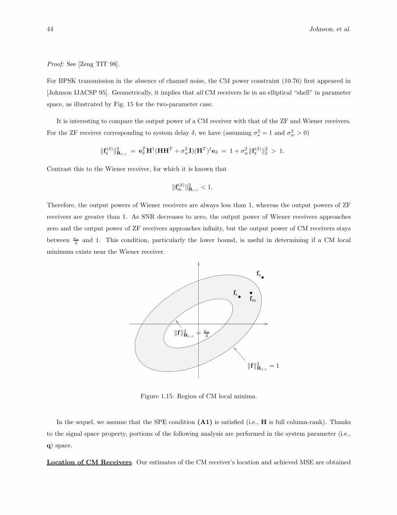
44 Johnson, et al.
Proof: See [Zeng TIT 98].
For BPSK transmission in the absence of channel noise, the CM power constraint (10.76) first appeared in
[Johnson IJACSP 95]. Geometrically, it implies that all CM receivers lie in an elliptical “shell” in parameter
space, as illustrated by Fig. 15 for the two-parameter case.
It is interesting to compare the output power of a CM receiver with that of the ZF and Wiener receivers.
For the ZF receiver corresponding to system delay δ, we have (assuming σ2s = 1 and σ2
w > 0)
‖f (δ)z ‖2
Rr,r= eT
δ H†(HHT + σ2wI)(HT )†eδ = 1 + σ2
w‖f (δ)z ‖2
2 > 1.
Contrast this to the Wiener receiver, for which it is known that
‖f (δ)m ‖2
Rr,r< 1.
Therefore, the output powers of Wiener receivers are always less than 1, whereas the output powers of ZF
receivers are greater than 1. As SNR decreases to zero, the output power of Wiener receivers approaches
zero and the output power of ZF receivers approaches infinity, but the output power of CM receivers stays
between κs
3 and 1. This condition, particularly the lower bound, is useful in determining if a CM local
minimum exists near the Wiener receiver.
‖f‖2Rr,r
= 1
‖f‖2Rr,r
= κs
3
fz
fmfc
Figure 1.15: Region of CM local minima.
In the sequel, we assume that the SPE condition (A1) is satisfied (i.e., H is full column-rank). Thanks
to the signal space property, portions of the following analysis are performed in the system parameter (i.e.,
q) space.
Location of CM Receivers. Our estimates of the CM receiver’s location and achieved MSE are obtained
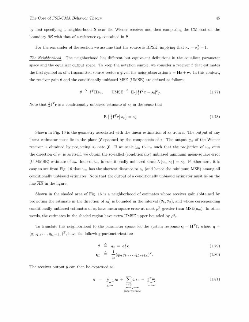
The Core of FSE-CMA Behavior Theory 45
by first specifying a neighborhood B near the Wiener receiver and then comparing the CM cost on the
boundary ∂B with that of a reference qr contained in B.
For the remainder of the section we assume that the source is BPSK, implying that κs = σ2s = 1.
The Neighborhood . The neighborhood has different but equivalent definitions in the equalizer parameter
space and the equalizer output space. To keep the notation simple, we consider a receiver f that estimates
the first symbol s0 of a transmitted source vector s given the noisy observation r = Hs+w. In this context,
the receiver gain θ and the conditionally unbiased MSE (UMSE) are defined as follows:
θ∆= fT He0, UMSE
∆= E
{|1θ f
T r − s0|2}. (1.77)
Note that 1θ f
T r is a conditionally unbiased estimate of s0 in the sense that
E{
1θ f
T r∣∣ s0
}= s0. (1.78)
Shown in Fig. 16 is the geometry associated with the linear estimation of s0 from r. The output of any
linear estimator must lie in the plane Y spanned by the components of r. The output ym of the Wiener
receiver is obtained by projecting s0 onto Y. If we scale ym to um such that the projection of um onto
the direction of s0 is s0 itself, we obtain the so-called (conditionally) unbiased minimum mean-square error
(U-MMSE) estimate of s0. Indeed, um is conditionally unbiased since E{um|s0} = s0. Furthermore, it is
easy to see from Fig. 16 that um has the shortest distance to s0 (and hence the minimum MSE) among all
conditionally unbiased estimates. Note that the output of a conditionally unbiased estimator must lie on the
line AB in the figure.
Shown in the shaded area of Fig. 16 is a neighborhood of estimates whose receiver gain (obtained by
projecting the estimate in the direction of s0) is bounded in the interval (θL, θU), and whose corresponding
conditionally unbiased estimates of s0 have mean-square error at most ρ2U greater than MSE(um). In other
words, the estimates in the shaded region have extra UMSE upper bounded by ρ2U.
To translate this neighborhood to the parameter space, let the system response q = HT f , where q =
(q0, q1, . . . , qLf+Lh)T , have the following parameterization:
θ∆= q0 = eT
0 q (1.79)
qI∆=
1
q0(q0, q1, . . . , qLf+Lh
)T . (1.80)
The receiver output y can then be expressed as
y = θ ·︸︷︷︸
gain
s0 +∑
i6=0
qisi
︸ ︷︷ ︸
interference
+ fTw︸︷︷︸
noise
, (1.81)
46 Johnson, et al.
θL
θ rθm
θU
yr ym
ρU
0
s0
um
A
B
Observation space Y
Figure 1.16: The region B in the Hilbert space of the observations.
where θ is the receiver gain, or bias. Scaling y by 1/θ, we have the (conditionally) unbiased estimate of s0:
u∆=
y
θ= s0 +
1
θ(∑
i6=0
qisi + fTw)
︸ ︷︷ ︸
equivalent noise
. (1.82)
Therefore, the receiver gain and UMSE of q is given by θ and MSE(u) respectively. Hence, the shaded
neighborhood in Fig. 16 can be described as
{q : θL < θ < θU, MSE(u) − MSE(um) < ρ2U}. (1.83)
In this definition, θL (θU) specifies the lower (upper) bound on CM receiver gain, while ρ2U specifies the upper
bound on extra UMSE.
Although the neighborhood defined above is related to specific characteristics of a receiver (i.e., UMSE
and bias), its relationship to the receiver coefficients (q) is not given explicitly. To locate the CM receiver
using this neighborhood, it is necessary to translate the neighborhood above to one that is specified in terms
of the system parameter space. Given the Wiener receiver qm = θm
(1
qmI
), it can be shown [Zeng TIT 98]
that an equivalent neighborhood, illustrated in the parameter space by Fig. 17, is given by
B(qm, ρU, θL, θU)∆= {q : θL < θ < θU, ‖qI − qmI‖C < ρU} (1.84)
= {q : θL < θ < θU, MSE(u) − MSE(um) < ρ2U}, (1.85)
where matrix C is a matrix formed by removing the first row and column from(I + σ2
wH†(H†)T).
The Reference qr. In relating the CM receiver to its Wiener counterpart, we choose, in the direction of the
Wiener receiver qm = θm
(1
qmI
), the reference point
qr∆= θr
1
qmI
(1.86)

The Core of FSE-CMA Behavior Theory 47
θqI
θL θr θm θU 1 θ
qr
qm ρU
Figure 1.17: A cone-type region: B(qm, ρU, θL, θU).
with the minimum CM cost. In other words, θr is chosen to minimize the CM cost of q = θ(
1qmI
)with
respect to θ, which can be shown to obey
θ2r =
θm
3 − 2θ2m − 2θ2
m‖qmI‖44
. (1.87)
In analyzing CM local minima in the neighborhood of Wiener receivers, the role of qr turns out to be more
than only technical: it can be shown that qr is a very good approximation of the CM receiver.
The theorem below provides us with a test for the existence of a CM receiver in B(qm, ρU, θL, θU).
Theorem 1.2 Given the Wiener receiver qm = θm
(1
qmI
)and the neighborhood B(qm, ρU, θL, θU) defined in
(10.84), define
D(ρ)∆= c1(ρ)2 − 4c2(ρ)c0, (1.88)
where
c0 =1
3 − 2θ2m − 2θ2
m‖qmI‖44
, (1.89)
c1(ρ) = −2(ρ2 +1
θm), (1.90)
c2(ρ) = 3(ρ2 +1
θm)2 − 2(1 + (ρ + ‖qmI‖4)
4). (1.91)
Under the conditions that MMSE < 13 and D(‖qmI‖2) < 0, a CM local minimum exists in the neighborhood
Bp(qm, ρ∗U, θ∗L, θ∗U). Here, ρ∗U is the smallest positive root of D(ρ), and
θ∗L = min0≤ρ≤ρ∗
U
√
−c1(ρ) −√
c1(ρ)2 − 4c2(ρ)c0
2c2(ρ), (1.92)
θ∗U = max0≤ρ≤ρ∗
U
√
−c1(ρ) +√
c1(ρ)2 − 4c2(ρ)c0
2c2(ρ). (1.93)
Furthermore, as the noise power decreases
limσw→0
Bp(qm, ρ∗U, θ∗L, θ∗U) = limσw→0
qc = limσw→0
qm = qz. (1.94)
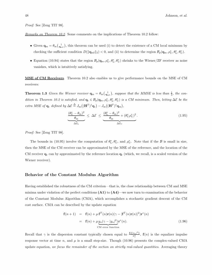
48 Johnson, et al.
Proof: See [Zeng TIT 98].
Remarks on Theorem 10.2. Some comments on the implications of Theorem 10.2 follow:
• Given qm = θm
(1
qmI
), this theorem can be used (i) to detect the existence of a CM local minimum by
checking the sufficient condition D(‖qmI‖2) < 0, and (ii) to determine the region Bp(qm, ρ∗U, θ∗L, θ∗U).
• Equation (10.94) states that the region Bp(qm, ρ∗U, θ∗L, θ∗U) shrinks to the Wiener/ZF receiver as noise
vanishes, which is intuitively satisfying.
MSE of CM Receivers. Theorem 10.2 also enables us to give performance bounds on the MSE of CM
receivers:
Theorem 1.3 Given the Wiener receiver qm = θm
(1
qmI
), suppose that the MMSE is less than 1
3 , the con-
dition in Theorem 10.2 is satisfied, and qc ∈ Bp(qm, ρ∗U, θ∗L, θ∗U) is a CM minimum. Then, letting ∆E be the
extra MSE of qc defined by ∆E ∆= Jm
((HT )†qc
)− Jm
((HT )†qm
),
(θ∗U − θm)2
θm︸ ︷︷ ︸
∆EL
≤ ∆E ≤ (θ∗L − θm)2
θm+ (θ∗Uρ∗U)2
︸ ︷︷ ︸
∆EU
. (1.95)
Proof: See [Zeng TIT 98].
The bounds in (10.95) involve the computation of θ∗L, θ∗U, and ρ∗U. Note that if the B is small in size,
then the MSE of the CM receiver can be approximated by the MSE of the reference, and the location of the
CM receiver qc can by approximated by the reference location qr (which, we recall, is a scaled version of the
Wiener receiver).
Behavior of the Constant Modulus Algorithm
Having established the robustness of the CM criterion—that is, the close relationship between CM and MSE
minima under violation of the perfect conditions (A1) to (A4)—we now turn to examination of the behavior
of the Constant Modulus Algorithm (CMA), which accomplishes a stochastic gradient descent of the CM
cost surface. CMA can be described by the update equation
f(n + 1) = f(n) + µ fT (n)r(n)(γ − |fT (n)r(n)|2)r∗(n)
= f(n) + µyn(γ − |yn|2)︸ ︷︷ ︸
CM error function
r∗(n). (1.96)
Recall that γ is the dispersion constant typically chosen equal to E{|sn|4}σ2
s, f(n) is the equalizer impulse
response vector at time n, and µ is a small step-size. Though (10.96) presents the complex-valued CMA
update equation, we focus the remainder of the section on strictly real-valued quantities. Averaging theory

The Core of FSE-CMA Behavior Theory 49
[Benveniste Book 90, Ljung Book 83] predicts that a SGD algorithm such as CMA converges almost surely
and in mean to the local minima of its cost surface (i.e., the CM receivers).
The performance of CMA can be categorized by its transient and steady-state behaviors. The multimodal
nature of the CM cost surface makes analysis of CMA transient behavior (e.g., the rate of convergence to
steady-state operation) more difficult than with unimodal linear-equalizer update algorithms such as LMS.
CMA’s steady-state behavior is characterized by parameter “jitter” around the (local) CM receiver, resulting
in non-zero excess CM-cost. In certain cases, the excess CM-cost can be translated directly into excess MSE,
a popular measure of adaptive equalizer performance. These topics are discussed in more detail in the
following subsections.
Transient Behavior: Convergence Rate. From a given initialization, CMA updates the equalizer by
descending the CM cost surface according to estimates of the direction of steepest descent. Due to the multi-
modality of Jcm, the convergence time (viewed as the number of iterations to reach “steady-state” behavior)
is greatly affected by equalizer initialization. Consequently, very few studies exist on CMA convergence rate,
[Larimore ICASSP 83], [Touzni EUSIPCO 96], and [Lambotharan SP 97] being exceptions.
To analyze CMA convergence, we consider the average CMA trajectories, or in other words, the tra-
jectories following an (exact) gradient descent of the CM cost surface in equalizer space. For a very small
step-size µ, a SGD algorithm of the form
f(n + 1) = f(n) + µF(f(n), r(n)
)
closely follows the average system (see [Benveniste Book 90, Ljung Book 83]) described by the ordinary
differential equation (ODE):
df(t)
dt= F (f),
where F (f) = E{F(f , r(n)
)}represents the mean update term of the algorithm and where t is a continuous
variable proportional to n.
In the absence of noise, CMA’s ODE can be derived from the mean CMA update term
E{r(n)f tr(n)(γ − |f tr(n)|2)
}= σ4
sH∆qq (recall (10.70)). Transforming to the system space, the ODE
becomes
dq
dt= Ht df
dt= σ4
sHtH∆qq. (1.97)
The trajectories resulting from the solution of (10.97) represent average paths for the evolution of q(n) when
updated by small step-size CMA. A display of some typical ODE trajectories is provided in Fig. 18.
Local Behavior . Under the PBE conditions and in the vicinity of a CM minimum (i.e., q ≈ eδ), the exact
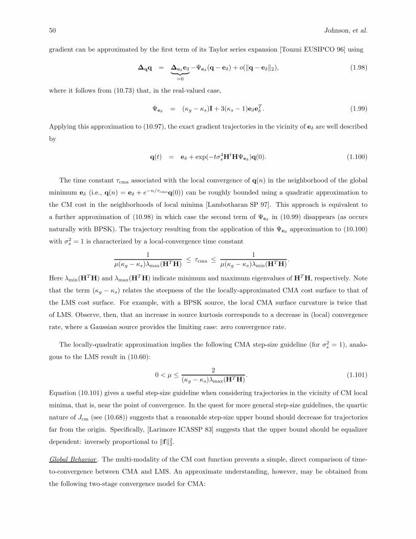
50 Johnson, et al.
gradient can be approximated by the first term of its Taylor series expansion [Touzni EUSIPCO 96] using
∆qq = ∆eδeδ
︸ ︷︷ ︸
=0
−Ψeδ(q − eδ) + o(‖q − eδ‖2), (1.98)
where it follows from (10.73) that, in the real-valued case,
Ψeδ= (κg − κs)I + 3(κs − 1)eδe
Tδ . (1.99)
Applying this approximation to (10.97), the exact gradient trajectories in the vicinity of eδ are well described
by
q(t) = eδ + exp(−tσ4sH
tHΨeδ)q(0). (1.100)
The time constant τcma associated with the local convergence of q(n) in the neighborhood of the global
minimum eδ (i.e., q(n) = eδ + e−n/τcmaq(0)) can be roughly bounded using a quadratic approximation to
the CM cost in the neighborhoods of local minima [Lambotharan SP 97]. This approach is equivalent to
a further approximation of (10.98) in which case the second term of Ψeδin (10.99) disappears (as occurs
naturally with BPSK). The trajectory resulting from the application of this Ψeδapproximation to (10.100)
with σ2s = 1 is characterized by a local-convergence time constant
1
µ(κg − κs)λmax(HTH)≤ τcma ≤ 1
µ(κg − κs)λmin(HT H).
Here λmin(HTH) and λmax(HT H) indicate minimum and maximum eigenvalues of HTH, respectively. Note
that the term (κg − κs) relates the steepness of the the locally-approximated CMA cost surface to that of
the LMS cost surface. For example, with a BPSK source, the local CMA surface curvature is twice that
of LMS. Observe, then, that an increase in source kurtosis corresponds to a decrease in (local) convergence
rate, where a Gaussian source provides the limiting case: zero convergence rate.
The locally-quadratic approximation implies the following CMA step-size guideline (for σ2s = 1), analo-
gous to the LMS result in (10.60):
0 < µ ≤ 2
(κg − κs)λmax(HT H). (1.101)
Equation (10.101) gives a useful step-size guideline when considering trajectories in the vicinity of CM local
minima, that is, near the point of convergence. In the quest for more general step-size guidelines, the quartic
nature of Jcm (see (10.68)) suggests that a reasonable step-size upper bound should decrease for trajectories
far from the origin. Specifically, [Larimore ICASSP 83] suggests that the upper bound should be equalizer
dependent: inversely proportional to ‖f‖22.
Global Behavior . The multi-modality of the CM cost function prevents a simple, direct comparison of time-
to-convergence between CMA and LMS. An approximate understanding, however, may be obtained from
the following two-stage convergence model for CMA:
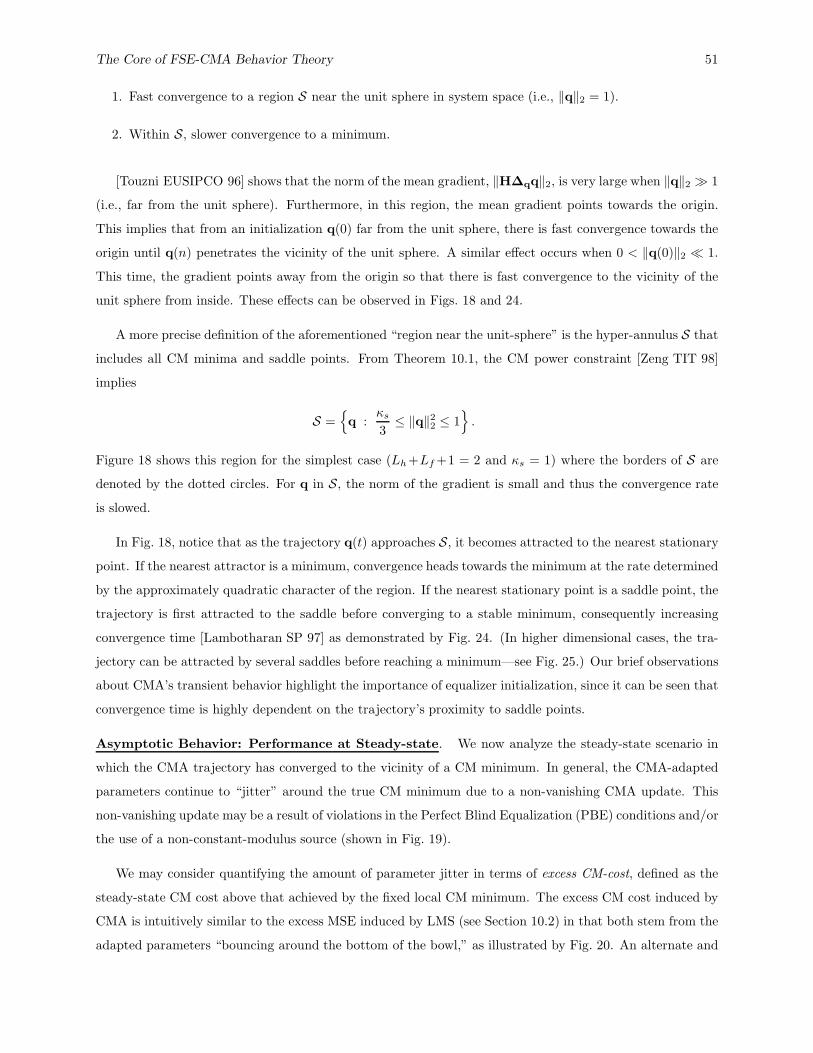
The Core of FSE-CMA Behavior Theory 51
1. Fast convergence to a region S near the unit sphere in system space (i.e., ‖q‖2 = 1).
2. Within S, slower convergence to a minimum.
[Touzni EUSIPCO 96] shows that the norm of the mean gradient, ‖H∆qq‖2, is very large when ‖q‖2 � 1
(i.e., far from the unit sphere). Furthermore, in this region, the mean gradient points towards the origin.
This implies that from an initialization q(0) far from the unit sphere, there is fast convergence towards the
origin until q(n) penetrates the vicinity of the unit sphere. A similar effect occurs when 0 < ‖q(0)‖2 � 1.
This time, the gradient points away from the origin so that there is fast convergence to the vicinity of the
unit sphere from inside. These effects can be observed in Figs. 18 and 24.
A more precise definition of the aforementioned “region near the unit-sphere” is the hyper-annulus S that
includes all CM minima and saddle points. From Theorem 10.1, the CM power constraint [Zeng TIT 98]
implies
S ={
q :κs
3≤ ‖q‖2
2 ≤ 1}
.
Figure 18 shows this region for the simplest case (Lh+Lf +1 = 2 and κs = 1) where the borders of S are
denoted by the dotted circles. For q in S, the norm of the gradient is small and thus the convergence rate
is slowed.
In Fig. 18, notice that as the trajectory q(t) approaches S, it becomes attracted to the nearest stationary
point. If the nearest attractor is a minimum, convergence heads towards the minimum at the rate determined
by the approximately quadratic character of the region. If the nearest stationary point is a saddle point, the
trajectory is first attracted to the saddle before converging to a stable minimum, consequently increasing
convergence time [Lambotharan SP 97] as demonstrated by Fig. 24. (In higher dimensional cases, the tra-
jectory can be attracted by several saddles before reaching a minimum—see Fig. 25.) Our brief observations
about CMA’s transient behavior highlight the importance of equalizer initialization, since it can be seen that
convergence time is highly dependent on the trajectory’s proximity to saddle points.
Asymptotic Behavior: Performance at Steady-state. We now analyze the steady-state scenario in
which the CMA trajectory has converged to the vicinity of a CM minimum. In general, the CMA-adapted
parameters continue to “jitter” around the true CM minimum due to a non-vanishing CMA update. This
non-vanishing update may be a result of violations in the Perfect Blind Equalization (PBE) conditions and/or
the use of a non-constant-modulus source (shown in Fig. 19).
We may consider quantifying the amount of parameter jitter in terms of excess CM-cost, defined as the
steady-state CM cost above that achieved by the fixed local CM minimum. The excess CM cost induced by
CMA is intuitively similar to the excess MSE induced by LMS (see Section 10.2) in that both stem from the
adapted parameters “bouncing around the bottom of the bowl,” as illustrated by Fig. 20. An alternate and

52 Johnson, et al.
−1.5 −1 −0.5 0 0.5 1 1.5−1.5
−1
−0.5
0
0.5
1
1.5
q0
q 1
(b)
−2 −1 0 1 2
−2
−1
0
1
2
f0
f 1
(a)
Figure 1.18: Exact gradient trajectories in (a) equalizer and (b) system space, with Lf = 0, Lh = 1 and
BPSK. Both figures show dotted hyper-annulus S boundaries and denote saddle points by ‘◦’ .
−2 −1 0 1 2−2
−1
0
1
2
Re
Im
8−PSK
−5 0 5−5
0
5
Re
Im
16−QAM
Figure 1.19: Non-constant modulus source constellation (16-QAM) versus constant modulus source constel-
lation (8-PSK).
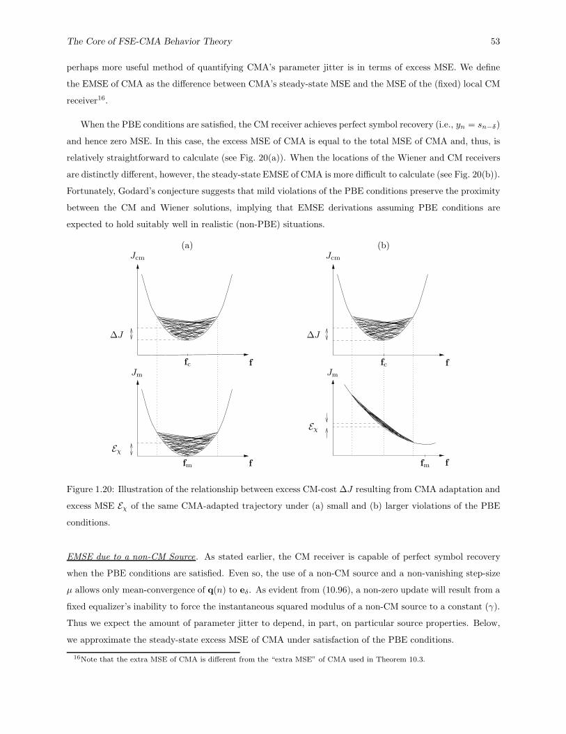
The Core of FSE-CMA Behavior Theory 53
perhaps more useful method of quantifying CMA’s parameter jitter is in terms of excess MSE. We define
the EMSE of CMA as the difference between CMA’s steady-state MSE and the MSE of the (fixed) local CM
receiver16.
When the PBE conditions are satisfied, the CM receiver achieves perfect symbol recovery (i.e., yn = sn−δ)
and hence zero MSE. In this case, the excess MSE of CMA is equal to the total MSE of CMA and, thus, is
relatively straightforward to calculate (see Fig. 20(a)). When the locations of the Wiener and CM receivers
are distinctly different, however, the steady-state EMSE of CMA is more difficult to calculate (see Fig. 20(b)).
Fortunately, Godard’s conjecture suggests that mild violations of the PBE conditions preserve the proximity
between the CM and Wiener solutions, implying that EMSE derivations assuming PBE conditions are
expected to hold suitably well in realistic (non-PBE) situations.
ff
f f
fmfm
fcfc
Eχ
Eχ
∆J∆J
JcmJcm
JmJm
(a) (b)
Figure 1.20: Illustration of the relationship between excess CM-cost ∆J resulting from CMA adaptation and
excess MSE Eχ of the same CMA-adapted trajectory under (a) small and (b) larger violations of the PBE
conditions.
EMSE due to a non-CM Source. As stated earlier, the CM receiver is capable of perfect symbol recovery
when the PBE conditions are satisfied. Even so, the use of a non-CM source and a non-vanishing step-size
µ allows only mean-convergence of q(n) to eδ. As evident from (10.96), a non-zero update will result from a
fixed equalizer’s inability to force the instantaneous squared modulus of a non-CM source to a constant (γ).
Thus we expect the amount of parameter jitter to depend, in part, on particular source properties. Below,
we approximate the steady-state excess MSE of CMA under satisfaction of the PBE conditions.
16Note that the extra MSE of CMA is different from the “extra MSE” of CMA used in Theorem 10.3.
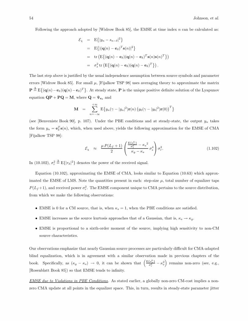
54 Johnson, et al.
Following the approach adopted by [Widrow Book 85], the EMSE at time index n can be calculated as:
Eχ = E{|yn − sn−δ|2
}
= E{|(q(n) − eδ)
T s(n)|2}
= tr(E{(q(n) − eδ)(q(n) − eδ)
T s(n)s(n)T})
= σ2s tr
(E{(q(n) − eδ)(q(n) − eδ)
T})
.
The last step above is justified by the usual independence assumption between source symbols and parameter
errors [Widrow Book 85]. For small µ, [Fijalkow TSP 98] uses averaging theory to approximate the matrix
P∆= E
{(q(n)−eδ)(q(n)−eδ)
T}. At steady state, P is the unique positive definite solution of the Lyapunov
equation QP + PQ = M, where Q = Ψeδand
M =+∞∑
n=−∞
E{yn(γ − |yn|2)r(n)
(y0(γ − |y0|2)r(0)
)T}
(see [Benveniste Book 90], p. 107). Under the PBE conditions and at steady-state, the output yn takes
the form yn = eTδ s(n), which, when used above, yields the following approximation for the EMSE of CMA
[Fijalkow TSP 98]:
Eχ ≈ µ P (Lf + 1)
2
E{s6n}
σ6s
− κs2
κg − κsσ4
s
σ2r . (1.102)
In (10.102), σ2r
∆= E{|rk|2} denotes the power of the received signal.
Equation (10.102), approximating the EMSE of CMA, looks similar to Equation (10.63) which approx-
imated the EMSE of LMS. Note the quantities present in each: step-size µ, total number of equalizer taps
P (Lf +1), and received power σ2r . The EMSE component unique to CMA pertains to the source distribution,
from which we make the following observations:
• EMSE is 0 for a CM source, that is, when κs = 1, when the PBE conditions are satisfied.
• EMSE increases as the source kurtosis approaches that of a Gaussian, that is, κs → κg.
• EMSE is proportional to a sixth-order moment of the source, implying high sensitivity to non-CM
source characteristics.
Our observations emphasize that nearly Gaussian source processes are particularly difficult for CMA-adapted
blind equalization, which is in agreement with a similar observation made in previous chapters of the
book. Specifically, as (κg − κs) → 0, it can be shown that(
E{s6n}
σ6s
− κ2s
)
remains non-zero (see, e.g.,
[Rosenblatt Book 85]) so that EMSE tends to infinity.
EMSE due to Violations in PBE Conditions . As stated earlier, a globally non-zero CM-cost implies a non-
zero CMA update at all points in the equalizer space. This, in turn, results in steady-state parameter jitter

The Core of FSE-CMA Behavior Theory 55
around CM local minima and yields non-zero steady-state excess CM-cost. Recall that violation of any of
the PBE conditions (A1)-(A3) yields the following:
• CM minima have CM-cost greater than zero.
• Not all CM minima yield the same CM-cost.
• CM receivers are no longer equivalent to MMSE or ZF receivers.
Hence, we conclude that any of the following: channel undermodelling, lack of subchannel disparity, the
presence of channel noise, or the use of a temporally correlated source will increase the steady-state level of
excess CM-cost. An example is presented in Section 10.4, where the difference between the dashed and solid
lines in Figs. 23(d)-(f) reveals EMSE due to noise, undermodelling, and nearly-common subchannel roots.
The fact that the CM cost surface is nearly quadratic in the vicinity of local minima suggests that the
excess CM-cost for CMA should be proportional to the same factors determining EMSE for LMS: step-size,
equalizer length, received signal power, and CM-cost at the minimum. Unfortunately, translating this excess
CM-cost into excess MSE is not always straightforward, especially for significant violations in the PBE
conditions (recall Fig. 20). This is due in part to the fact that we lack closed-form expressions for the CM
receivers when any of the conditions (A1)-(A3) is violated. To summarize, a method of quantifying the
EMSE of CMA under arbitrary violation of the PBE conditions remains an open problem.
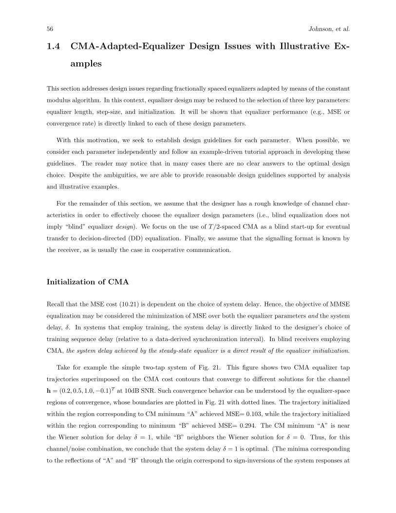
56 Johnson, et al.
1.4 CMA-Adapted-Equalizer Design Issues with Illustrative Ex-
amples
This section addresses design issues regarding fractionally spaced equalizers adapted by means of the constant
modulus algorithm. In this context, equalizer design may be reduced to the selection of three key parameters:
equalizer length, step-size, and initialization. It will be shown that equalizer performance (e.g., MSE or
convergence rate) is directly linked to each of these design parameters.
With this motivation, we seek to establish design guidelines for each parameter. When possible, we
consider each parameter independently and follow an example-driven tutorial approach in developing these
guidelines. The reader may notice that in many cases there are no clear answers to the optimal design
choice. Despite the ambiguities, we are able to provide reasonable design guidelines supported by analysis
and illustrative examples.
For the remainder of this section, we assume that the designer has a rough knowledge of channel char-
acteristics in order to effectively choose the equalizer design parameters (i.e., blind equalization does not
imply “blind” equalizer design). We focus on the use of T/2-spaced CMA as a blind start-up for eventual
transfer to decision-directed (DD) equalization. Finally, we assume that the signalling format is known by
the receiver, as is usually the case in cooperative communication.
Initialization of CMA
Recall that the MSE cost (10.21) is dependent on the choice of system delay. Hence, the objective of MMSE
equalization may be considered the minimization of MSE over both the equalizer parameters and the system
delay, δ. In systems that employ training, the system delay is directly linked to the designer’s choice of
training sequence delay (relative to a data-derived synchronization interval). In blind receivers employing
CMA, the system delay achieved by the steady-state equalizer is a direct result of the equalizer initialization.
Take for example the simple two-tap system of Fig. 21. This figure shows two CMA equalizer tap
trajectories superimposed on the CMA cost contours that converge to different solutions for the channel
h = (0.2, 0.5, 1.0,−0.1)T at 10dB SNR. Such convergence behavior can be understood by the equalizer-space
regions of convergence, whose boundaries are plotted in Fig. 21 with dotted lines. The trajectory initialized
within the region corresponding to CM minimum “A” achieved MSE= 0.103, while the trajectory initialized
within the region corresponding to minimum “B” achieved MSE= 0.294. The CM minimum “A” is near
the Wiener solution for delay δ = 1, while “B” neighbors the Wiener solution for δ = 0. Thus, for this
channel/noise combination, we conclude that the system delay δ = 1 is optimal. (The minima corresponding
to the reflections of “A” and “B” through the origin correspond to sign-inversions of the system responses at
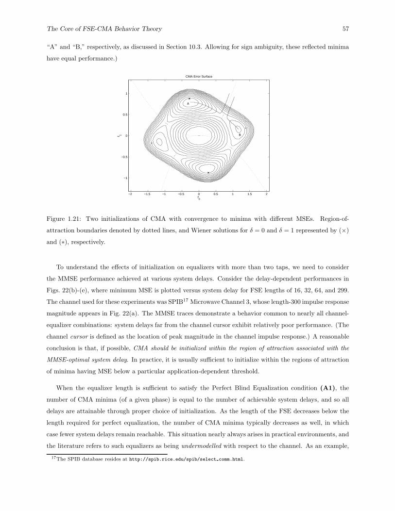
The Core of FSE-CMA Behavior Theory 57
“A” and “B,” respectively, as discussed in Section 10.3. Allowing for sign ambiguity, these reflected minima
have equal performance.)
−2 −1.5 −1 −0.5 0 0.5 1 1.5 2
−1
−0.5
0
0.5
1
f0
f 1
CMA Error Surface
A
B
Figure 1.21: Two initializations of CMA with convergence to minima with different MSEs. Region-of-
attraction boundaries denoted by dotted lines, and Wiener solutions for δ = 0 and δ = 1 represented by (×)
and (∗), respectively.
To understand the effects of initialization on equalizers with more than two taps, we need to consider
the MMSE performance achieved at various system delays. Consider the delay-dependent performances in
Figs. 22(b)-(e), where minimum MSE is plotted versus system delay for FSE lengths of 16, 32, 64, and 299.
The channel used for these experiments was SPIB17 Microwave Channel 3, whose length-300 impulse response
magnitude appears in Fig. 22(a). The MMSE traces demonstrate a behavior common to nearly all channel-
equalizer combinations: system delays far from the channel cursor exhibit relatively poor performance. (The
channel cursor is defined as the location of peak magnitude in the channel impulse response.) A reasonable
conclusion is that, if possible, CMA should be initialized within the region of attraction associated with the
MMSE-optimal system delay. In practice, it is usually sufficient to initialize within the regions of attraction
of minima having MSE below a particular application-dependent threshold.
When the equalizer length is sufficient to satisfy the Perfect Blind Equalization condition (A1), the
number of CMA minima (of a given phase) is equal to the number of achievable system delays, and so all
delays are attainable through proper choice of initialization. As the length of the FSE decreases below the
length required for perfect equalization, the number of CMA minima typically decreases as well, in which
case fewer system delays remain reachable. This situation nearly always arises in practical environments, and
the literature refers to such equalizers as being undermodelled with respect to the channel. As an example,
17The SPIB database resides at http://spib.rice.edu/spib/select comm.html.
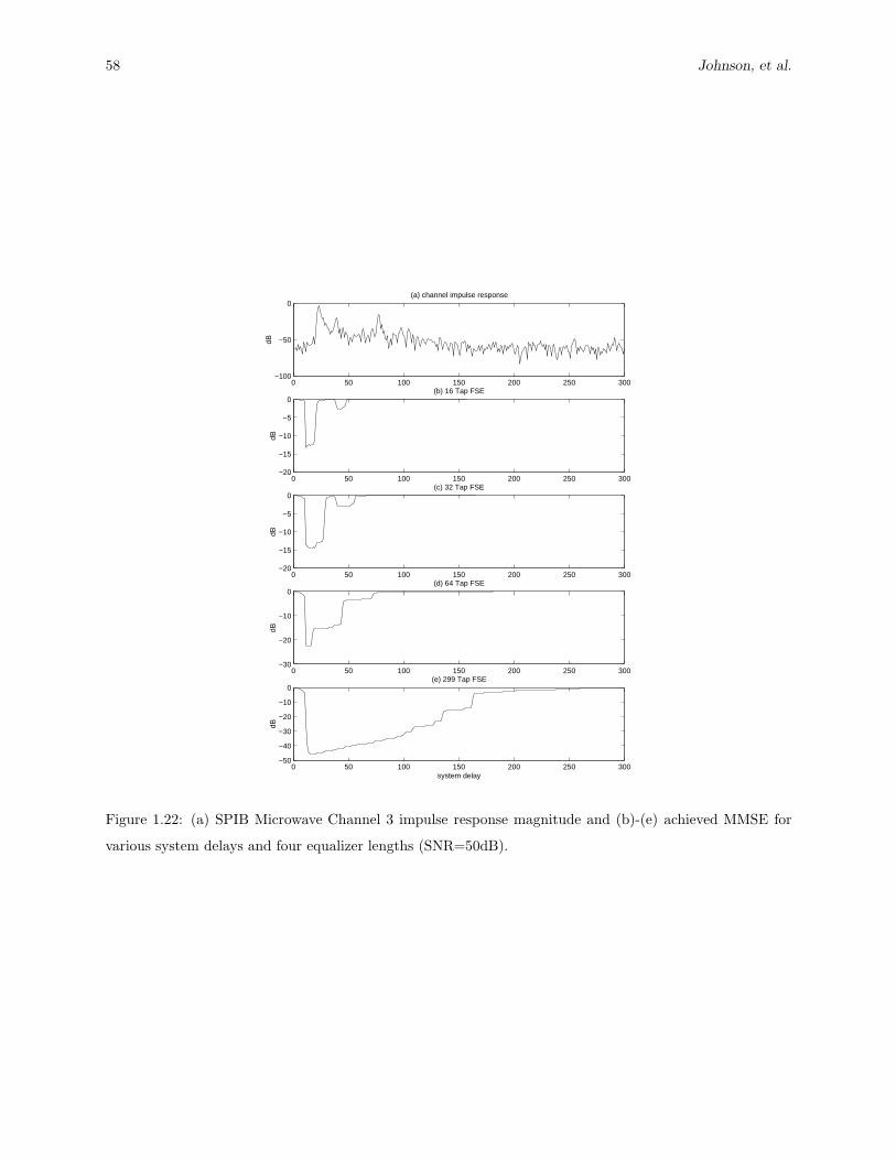
58 Johnson, et al.
0 50 100 150 200 250 300−100
−50
0
dB
(a) channel impulse response
0 50 100 150 200 250 300−20
−15
−10
−5
0
dB
(b) 16 Tap FSE
0 50 100 150 200 250 300−20
−15
−10
−5
0
dB
(c) 32 Tap FSE
0 50 100 150 200 250 300−30
−20
−10
0
dB
(d) 64 Tap FSE
0 50 100 150 200 250 300−50
−40
−30
−20
−10
0
dB
(e) 299 Tap FSE
system delay
Figure 1.22: (a) SPIB Microwave Channel 3 impulse response magnitude and (b)-(e) achieved MMSE for
various system delays and four equalizer lengths (SNR=50dB).
The Core of FSE-CMA Behavior Theory 59
Fig. 11 shows one CMA solution near two sub-optimal Wiener solutions, while the other CMA solution
remains near the Wiener receiver of optimal delay. Ideally, we would like the limited set of reachable delays
to be those that achieve the best MMSE performance. Our claim is that undermodelled FSE-CMA typically
provides this desired behavior, at least using popular initialization strategies. Before substantiating this
claim, however, we will discuss these initialization strategies.
Single-Spike Initialization. The most common strategy for initialization of CMA is termed single-spike
initialization and derives its name from the baud-spaced strategy first suggested in [Godard TCOM 80]. The
single-spike technique specifies that all but one of the BSE coefficients are set to zero, though the location
and amplitude of the nonzero tap has long been a subject of debate. Recently, [Chung ASIL 98] made
the observation that initializations with small norm result in almost certain CMA convergence to “good”
local minima, that is, CM minima associated with relatively good MSE performance. Figure 21 illustrates
this phenomenon for a 2-tap FSE: note how the regions of attraction corresponding to the better minima
completely dominate the area near the origin. Unfortunately, the fact that the origin is a local maximum
of the CM cost surface implies that initializations with extremely small norm will result in slow (initial)
convergence. It has been found that, in practical18 situations, an initialization norm ‖finit‖2 ≈ 1 is usually
a good compromise between convergence rate and region-of-attraction selection.
The single-spike strategy as described above is not always appropriate for fractionally-spaced equalizers.
For example, consider the trivial T/2-spaced channel h = (0, 1, 0, 0)T with the single-spike FSE initialization
f = (0, 1)T . If the equalizer output is decimated such that the odd-indexed samples are retained, then
the equalizer output (and hence the CMA update) will be zero! In other words, the subchannel providing
the signal energy will be nulled by the initial equalizer. What might be a more appropriate T/2-spaced
initialization strategy is known as double-spike initialization and contains non-zero components in both
subequalizers. Note that choosing the non-zero tap magnitudes ≈ 1/√
2 will result in an equalizer norm ≈ 1.
It is customary to place the non-zero fractionally-spaced taps adjacent to one another. This practice may
be justified in the frequency domain, as adjacent positioning results in an initialization spectrum similar to
a raised-cosine-pulse matched filter. The relative placement of the adjacent tap pair will be the focus of an
upcoming subsection.
Relationship between FSE-Length and Initialization Sensitivity. At this point we return to our
discussion of initialization for undermodelled equalizers. (Recall that undermodelling nearly always exists in
practice.) Previously we claimed that, under a reasonable initialization, FSE-CMA achieves a “good” range
of reachable system delays. Using the unit-norm double-spike initialization strategy, we now offer example
evidence for this claim19. Figure 23 shows steady-state MSE performance achieved by CMA for the full range
18We assume that the received signal power is unit-normalized by automatic gain control prior to equalization.19As no rigorous proofs of optimality exist for the single/double-spike initialization scheme, we are not claiming that the
reachable set of delays is always optimal. However, practitioners have found these initialization strategies to work well.

60 Johnson, et al.
of (adjacent) double-spike locations. For ease of comparison, the same channel and equalizer lengths used in
Fig. 22 are used. Other details include the use of QPSK, a SNR of 50 dB, step-sizes {0.005, 0.005, 0.0025} for
respective FSE lengths {16, 32, 64}, and simulation lengths of 106 iterations. Figure 23 has two important
0 5 1012
14
16
18
20
spike loc
dela
y(a) 16 Tap
0 10 20 3010
15
20
25
30
spike locde
lay
(b) 32 Tap
0 20 40 6010
20
30
40
50
spike loc
dela
y
(c) 64 Tap
0 5 10−13
−12
−11
spike loc
dB
(d) 16 Tap
0 10 20 30−15
−14
−13
−12
−11
−10
spike loc
dB
(e) 32 Tap
0 20 40 60−25
−20
−15
−10
spike loc
dB
(f) 64 Tap
Figure 1.23: (a)-(c) Achieved system delay as a function of double-spike location and (d)-(f) CMA’s corre-
sponding MSE performance for the channel response in Fig. 22(a). The dashed lines indicate Wiener (i.e.,
MMSE) performance at the respective system delays.
messages:
• First, the only system delays reached by FSE-CMA under double-spike initialization were indeed those
corresponding to the low-MMSE “troughs” in Fig. 22; FSE-CMA avoided convergence to system delays
characterized by poor MMSE. (Notice that the dashed lines in Figs. 23(d)-(f) correspond to the lowest
sections of the MMSE traces in Fig. 22.)
• Second, the relative MSE performance versus delay seems to “even out” as the degree of undermodelling
increases. In other words, initialization sensitivity decreases as equalizer length decreases. Note,
however, that for the same (nonzero) noise level, the MMSE performance achieved by shorter equalizers
is typically20 worse. In fact, the best MSE achieved by the 16-tap CMA-adapted equalizer in Fig. 23
is not as good as the worst MSE achieved by the 64-tap equalizer.
20Due to the effects of EMSE, longer adaptive equalizers will not always result in lower steady state EMSE, as discussed in
Section 10.4 and illustrated by Fig. 28.
The Core of FSE-CMA Behavior Theory 61
The shape of the typical “trough” in the MMSE-versus-delay profile [Larimore ICASSP 97] implies that,
even for long equalizers, good performance is assured when the initialization spike is chosen anywhere within
the region corresponding to the lowest-MMSE delay.
Spike-Delay Selection. We note from Figs. 23(a)-(c) that there seems to be a direct correspondence
between initial spike location and achieved system delay. A similar observation was made in [Li TSP 95] for
single-spike initialized BSEs. Thus, knowing something about the channel impulse response shape can help
with the selection of initialization. For example, if the channel impulse response is reasonably symmetric,
a center-spike is most appropriate. If, on the other hand, the channel impulse response is asymmetric (i.e.,
the center of mass is skewed towards the left or right), then the initial spike location should be moved in
the direction of the center of mass. An example is the channel response in Fig. 22(a), which is skewed very
much towards the left. The achieved MSE in Figs. 23(d)-(f) confirms that, for this channel, the initialization
spike locations toward the left yield better performance. Finally, when little or nothing is known about
the channel, the width of the MSE troughs in Figs. 23(d)-(f) suggests that as few as three double-spike
initializations (e.g., “left”, “center”, and “right”) might be sufficient for repeated attempts at a successful
initialization.
Attraction by Saddles. Unfortunately, location within a good region of convergence is not the only
requirement of an ideal CMA initialization. As it turns out, initialization can have a profound effect on
time-to-convergence. The potential for arbitrarily slow convergence can be explained by the existence of
saddle-points on the CM cost surface, that is, points with zero gradient that are concave along certain
directions and convex along others [Johnson IJACSP 95]. The convergence-slowing mechanism of saddle
points can be explained as follows: concavity attracts trajectories from particular directions, lack of local
gradient stalls the trajectories in the vicinity of the saddles, and convexity eventually ejects the trajectories
in other directions21. Figure 24 shows examples of this behavior for different two-tap FSE initializations
using the noiseless T/2-spaced channel response (0.2, 0.5, 1,−0.1)T and a BPSK source. Note that in this
two-dimensional example, the CMA trajectories are only capable of passing through one saddle before
converging to a stable minimum. Figure 25 plots the CM-cost evolution for a higher-dimensional case in
which the CMA trajectory passes near multiple saddles [Lambotharan SP 97]. Here the T/2-spaced channel
was h = (0.7571,−0.2175, 0.1010, 0.4185, 0.4038, 0.1762)T and the four-tap FSE was double-spike initialized
at f = (1, 1, 0, 0)T /√
2. Notice that even the popular double-spike initialization is susceptible to attraction
by saddles.
Indirect Initialization Techniques. If needed, the information gained from convergence to one CMA
solution can be used to better initialize a second attempt. For instance, [Tong SPL 97] proposes an iterative
scheme whereby a delay-shifted version of a channel estimate derived from one CMA-derived equalizer
21Technically speaking, the directions of attraction correspond to the eigenvectors of the Hessian associated with positive
eigenvalues, while the directions of repulsion correspond to the eigenvectors associated with negative eigenvalues.

62 Johnson, et al.
−2 −1 0 1 2
−1
−0.5
0
0.5
1
f0
f1CM Cost Surface
CB
A
0 2000 4000 6000−50
−40
−30
−20
−10
0
10CM Cost
dB
Iteration number
CBA
Figure 1.24: Two-tap FSE-CMA trajectories and CM-cost history for several initializations showing the
effect of a saddle point on convergence speed.
0 5000 10000 150000
0.1
0.2
0.3
0.4
0.5
0.6
0.7
Iteration number
CM
Cos
t
Attraction of second saddle
Attraction of first saddle
Figure 1.25: Slow convergence of a double-spike-initialized 4-tap FSE due to multiple saddle point attractions.
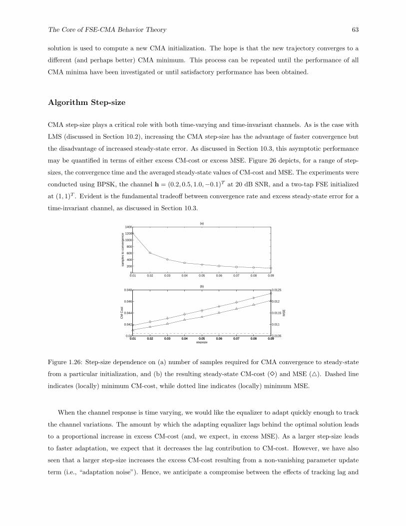
The Core of FSE-CMA Behavior Theory 63
solution is used to compute a new CMA initialization. The hope is that the new trajectory converges to a
different (and perhaps better) CMA minimum. This process can be repeated until the performance of all
CMA minima have been investigated or until satisfactory performance has been obtained.
Algorithm Step-size
CMA step-size plays a critical role with both time-varying and time-invariant channels. As is the case with
LMS (discussed in Section 10.2), increasing the CMA step-size has the advantage of faster convergence but
the disadvantage of increased steady-state error. As discussed in Section 10.3, this asymptotic performance
may be quantified in terms of either excess CM-cost or excess MSE. Figure 26 depicts, for a range of step-
sizes, the convergence time and the averaged steady-state values of CM-cost and MSE. The experiments were
conducted using BPSK, the channel h = (0.2, 0.5, 1.0,−0.1)T at 20 dB SNR, and a two-tap FSE initialized
at (1, 1)T . Evident is the fundamental tradeoff between convergence rate and excess steady-state error for a
time-invariant channel, as discussed in Section 10.3.
0.01 0.02 0.03 0.04 0.05 0.06 0.07 0.08 0.090
200
400
600
800
1000
1200
1400(a)
sam
ples
to c
onve
rgen
ce
0.01 0.02 0.03 0.04 0.05 0.06 0.07 0.08 0.090.04
0.042
0.044
0.046
0.048
CM
Cos
t
0.01 0.02 0.03 0.04 0.05 0.06 0.07 0.08 0.090.0105
0.011
0.0115
0.012
0.0125
MS
E(b)
stepsize
Figure 1.26: Step-size dependence on (a) number of samples required for CMA convergence to steady-state
from a particular initialization, and (b) the resulting steady-state CM-cost (�) and MSE (4). Dashed line
indicates (locally) minimum CM-cost, while dotted line indicates (locally) minimum MSE.
When the channel response is time varying, we would like the equalizer to adapt quickly enough to track
the channel variations. The amount by which the adapting equalizer lags behind the optimal solution leads
to a proportional increase in excess CM-cost (and, we expect, in excess MSE). As a larger step-size leads
to faster adaptation, we expect that it decreases the lag contribution to CM-cost. However, we have also
seen that a larger step-size increases the excess CM-cost resulting from a non-vanishing parameter update
term (i.e., “adaptation noise”). Hence, we anticipate a compromise between the effects of tracking lag and
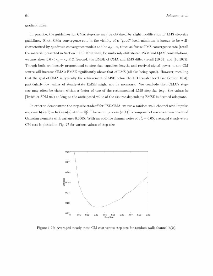
64 Johnson, et al.
gradient noise.
In practice, the guidelines for CMA step-size may be obtained by slight modification of LMS step-size
guidelines. First, CMA convergence rate in the vicinity of a “good” local minimum is known to be well-
characterized by quadratic convergence models and be κg −κs times as fast as LMS convergence rate (recall
the material presented in Section 10.3). Note that, for uniformly-distributed PAM and QAM constellations,
we may show 0.6 < κg − κs ≤ 2. Second, the EMSE of CMA and LMS differ (recall (10.63) and (10.102)).
Though both are linearly proportional to step-size, equalizer length, and received signal power, a non-CM
source will increase CMA’s EMSE significantly above that of LMS (all else being equal). However, recalling
that the goal of CMA is typically the achievement of MSE below the DD transfer level (see Section 10.4),
particularly low values of steady-state EMSE might not be necessary. We conclude that CMA’s step-
size may often be chosen within a factor of two of the recommended LMS step-size (e.g., the values in
[Treichler SPM 96]) so long as the anticipated value of the (source-dependent) EMSE is deemed adequate.
In order to demonstrate the step-size tradeoff for FSE-CMA, we use a random walk channel with impulse
response h(k+1) = h(k)+n(k) at time kT2 . The vector process {n(k)} is composed of zero-mean uncorrelated
Gaussian elements with variance 0.0005. With an additive channel noise of σ2w = 0.05, averaged steady-state
CM-cost is plotted in Fig. 27 for various values of step-size.
0 0.01 0.02 0.03 0.04 0.05 0.06 0.07 0.08 0.090.22
0.23
0.24
0.25
0.26
0.27
0.28
Step Size
CM
Cos
t
Figure 1.27: Averaged steady-state CM-cost versus step-size for random-walk channel h(k).

The Core of FSE-CMA Behavior Theory 65
Equalizer Length
Equalizer length is one of the most important variables in communication receiver system design. It is directly
related to both optimum receiver performance and implementation cost. For example, approximately 80%
of Applied Signal Technology’s VLSI chip described in [Treichler SPM 96] is devoted to the FSE.
A common myth regarding equalizer length selection is that a longer FSE always achieves better MSE
performance than a shorter FSE. This principle is false for equalizers adapted by a stochastic gradient
descent algorithm such as CMA. In the presence of channel noise, a longer FSE is better at mitigating the
effects of ISI and noise than a shorter FSE, but a longer FSE will incur the penalty of additional MSE due
to increased adaptation noise [Widrow PROC 76]. Although CMA and LMS both exhibit this undesirable
excess MSE (EMSE) due to adaptation noise (see Section 10.2), CMA suffers additional EMSE when used
with a non-CM source. (Recall from Section 10.3 that a non-CM source makes it impossible to achieve
zero CM cost, and it is this non-zero CM cost that causes the CMA-adapted FSE coefficients to “rattle
around” the locally-optimal CM solution when driven by a non-vanishing step-size.) The resulting EMSE
under the perfect blind equalization conditions was approximated in (10.102) and, as with LMS in (10.63),
is proportional to both step-size and FSE length. Herein lies the classical compromise: the FSE length
should be long enough to mitigate channel-induced noise and ISI but short enough to prevent the MSE due
to adaptation noise from dominating.
Combining the approximate effects of equalizer length and source kurtosis on MSE from
[Endres ICASSP 97] and (10.102), respectively, Fig. 28 presents steady-state MSE performance of CMA
for various equalizer lengths and step-sizes. The calculated data assumes a 16-QAM source over SPIB Mi-
crowave Channel 2 in the absence of noise. Our goal for the blind start-up mode is to choose a length/step-size
combination capable of achieving a MSE below the decision-directed (DD) transfer level. The dashed line in
Fig. 28 indicates this transfer level for 16-QAM. (Choosing the transfer level will be the subject of the next
section.) Figure 28 demonstrates that a longer equalizer does not necessarily provide better steady-state
performance than a shorter one. In fact, with certain channel/step-size combinations, an FSE-length less
than that required for perfect equalization may be required for CMA to reach the DD transfer level. A
similar observation was made for BSE-CMA in [Li TSP 96c].
So far we have focused on choosing equalizer length suited to the requirements of CMA in the blind
start-up mode. The behavior and requirements of LMS-adapted DD equalization, however, may lead to a
slightly different equalizer length tradeoff. For example, we have already noticed that LMS equalizers are not
affected by non-CM sources in the way that CMA equalizers are. In addition, the goal of the DD equalization
mode may be to attain a symbol error rate (SER) of ≤ 10−6, while the goal of CMA equalization might
only be to attain SER < 10−2. The differences between the start-up and DD modes suggest that it may be
useful to allow different equalizer lengths for the two modes. In general, the DD-adapted equalizer should
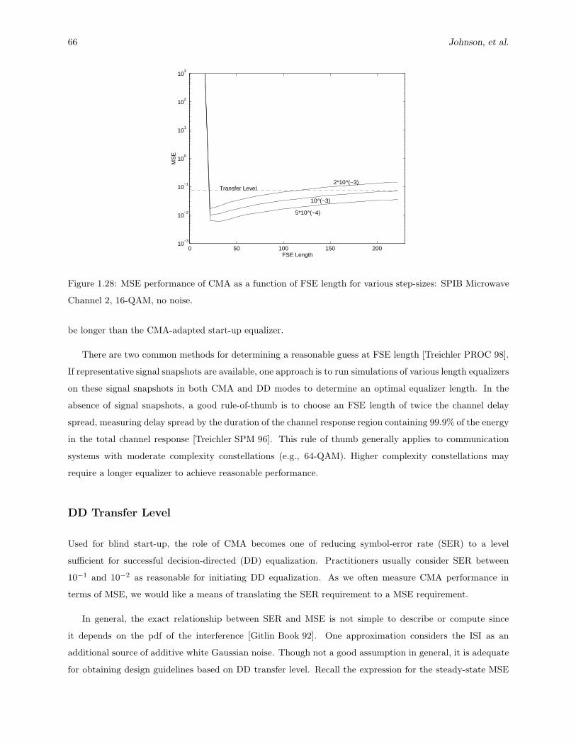
66 Johnson, et al.
0 50 100 150 20010
−3
10−2
10−1
100
101
102
103
FSE Length
MS
E
Transfer Level
5*10^(−4)
10^(−3)
2*10^(−3)
Figure 1.28: MSE performance of CMA as a function of FSE length for various step-sizes: SPIB Microwave
Channel 2, 16-QAM, no noise.
be longer than the CMA-adapted start-up equalizer.
There are two common methods for determining a reasonable guess at FSE length [Treichler PROC 98].
If representative signal snapshots are available, one approach is to run simulations of various length equalizers
on these signal snapshots in both CMA and DD modes to determine an optimal equalizer length. In the
absence of signal snapshots, a good rule-of-thumb is to choose an FSE length of twice the channel delay
spread, measuring delay spread by the duration of the channel response region containing 99.9% of the energy
in the total channel response [Treichler SPM 96]. This rule of thumb generally applies to communication
systems with moderate complexity constellations (e.g., 64-QAM). Higher complexity constellations may
require a longer equalizer to achieve reasonable performance.
DD Transfer Level
Used for blind start-up, the role of CMA becomes one of reducing symbol-error rate (SER) to a level
sufficient for successful decision-directed (DD) equalization. Practitioners usually consider SER between
10−1 and 10−2 as reasonable for initiating DD equalization. As we often measure CMA performance in
terms of MSE, we would like a means of translating the SER requirement to a MSE requirement.
In general, the exact relationship between SER and MSE is not simple to describe or compute since
it depends on the pdf of the interference [Gitlin Book 92]. One approximation considers the ISI as an
additional source of additive white Gaussian noise. Though not a good assumption in general, it is adequate
for obtaining design guidelines based on DD transfer level. Recall the expression for the steady-state MSE
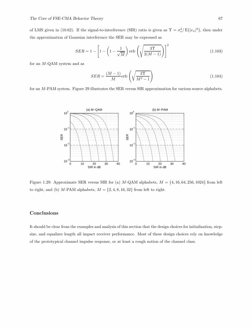
The Core of FSE-CMA Behavior Theory 67
of LMS given in (10.62). If the signal-to-interference (SIR) ratio is given as Υ = σ2s/ E{|en|2}, then under
the approximation of Gaussian interference the SER may be expressed as
SER = 1 −[
1 −(
1 − 1√M
)
erfc
(√
3Υ
2(M − 1)
)]2
(1.103)
for an M -QAM system and as
SER =(M − 1)
Merfc
(√
3Υ
M2 − 1
)
(1.104)
for an M -PAM system. Figure 29 illustrates the SER versus SIR approximation for various source alphabets.
0 10 20 30 4010
−3
10−2
10−1
100
SIR in dB
SE
R
(a) M−QAM
0 10 20 30 4010
−3
10−2
10−1
100
SIR in dB
SE
R
(b) M−PAM
Figure 1.29: Approximate SER versus SIR for (a) M -QAM alphabets, M = {4, 16, 64, 256, 1024} from left
to right, and (b) M -PAM alphabets, M = {2, 4, 8, 16, 32} from left to right.
Conclusions
It should be clear from the examples and analysis of this section that the design choices for initialization, step-
size, and equalizer length all impact receiver performance. Most of these design choices rely on knowledge
of the prototypical channel impulse response, or at least a rough notion of the channel class.

68 Johnson, et al.
1.5 Case Studies
To illustrate design methodology, we consider three actual communication scenarios addressing different
classes of channel impairments to digital transmissions. The first, the voiceband telephone channel, typically
has a high SNR and is dominated by transmission line effects and passive audio shaping. The second exam-
ple involves the coaxial cable channel carrying residential TV service. Over the normal channel allocation,
this broadband medium suffers both from noise/interference effects and dispersion due to analog mismatch-
ing. Lastly, we consider the terrestrial microwave radio channel, with its dynamic reflective multi-path
environment.
For each case we examine the specification of equalizer settings, such as step-size, FSE-length and ini-
tialization, from the varying degrees of a priori information available. Then, using actual received signal
snapshots, we examine CMA’s blind equalization performance in each case. Use of experimentally acquired
received data from actual communications channels also requires us to consider other issues such as carrier
frequency offset, noise, and channel time-variations. The effects of carrier frequency offset, to which CMA
is immune because of its independence of phase, will be illustrated in the voiceband modem example. The
digital cable television example will illustrate the effects of noise on blind equalization of large signal con-
stellations. The last example, mobile microwave communication, is characterized by a time-varying channel.
We will show how the three signal environments impact our equalizer parameter selection and equalizer
performance.
Good design practice requires us to define the equalizer using any information known about the particular
signal environment. For example, for a particular communications link, we may be able to characterize a
suitable range of equalizer lengths, communication channel delays, degree of time variation in the channel,
and range of SNR. To minimize hardware complexity and maximize agility, we would like to simultaneously
choose the shortest equalizer length, largest step-size, and most broadly successful initialization. While our
objective is to rapidly reduce the ISI to allow carrier tracking and switching to decision-directed equalization
in the least amount of time, practically we try to select the parameters to provide a solution allowing steady-
state decision-directed equalization within the constraints of the software and/or hardware being used to
process the data.
In the following examples, all of the channels are derived from empirical measurements by Applied Signal
Technology, Inc., and reside in the SPIB database at http://spib.rice.edu/spib/select comm.html.
Voiceband Modem: The Dial-up Telephone Channel
We first consider a class of channels that exhibits a wide range of challenging characteristics. Today, data
transmission over a dial-up telephone channel is taken for granted as an integral part of personal telecommu-

The Core of FSE-CMA Behavior Theory 69
nications, enabling, for example, the individual’s access to the Internet as well as widespread use of dialup
facsimile machines. The channel effects in such a transmission medium are due mainly to the analog “local
subscriber loop” originally engineered for speech service. This passive connection runs from the subscriber’s
premises to the telephone service provider’s local office facility. The signal must be carried over this copper
line, up to 5 km in length, subject not only to passive transmission line dispersion, but also to a variety of
non-ideal effects such as spliced wire gauges, non-terminated shunts, and dielectric variations. Once con-
nected to the public switched telephone network (PSTN), the signal occupies the voice band in the range
from 300 to 3400 Hz, with band-limiting sufficient to support the 8-kHz sampling operation used for TDM
in the digital switching and transmission system. The channel typically exhibits phase irregularities near
band edges, with a sloping or rippling magnitude loss on the upper half of the passband; Fig. 30(a) shows
the magnitude response for a typical voiceband channel.
0 500 1000 1500 2000 2500 3000 3500 4000−15
−10
−5(a)
Hz
dB
0 2 4 6 8 10 12−35
−30
−25
−20
−15
−10
−5
0
ms
dB
(b)
Figure 1.30: Prototypical voiceband channel: (a) frequency response magnitude, (b) impulse response mag-
nitude.
Assuring reliable transmission of data under such conditions has proven very challenging and has moti-
vated some of the earliest endeavors in adaptive equalization and coded modulation. The nature of the basic
channel limits symbol rate to on the order of 3400 symbols/sec, with modulating carrier frequency between
1700 and 1900 Hz. Furthermore, the complexity of QAM modulation, hence the actual data rate, is limited
mainly by severe ISI rather than additive noise, since the SNR typically exceeds 30 dB. Because the channel
characteristics may vary widely from connection to connection, equalization of so-called “dial-up” service
by the receiving terminal must be highly robust. This often involves automatic training options that not
only initialize equalizer parameters but also allow adjustment of modulation symbol rate and constellation
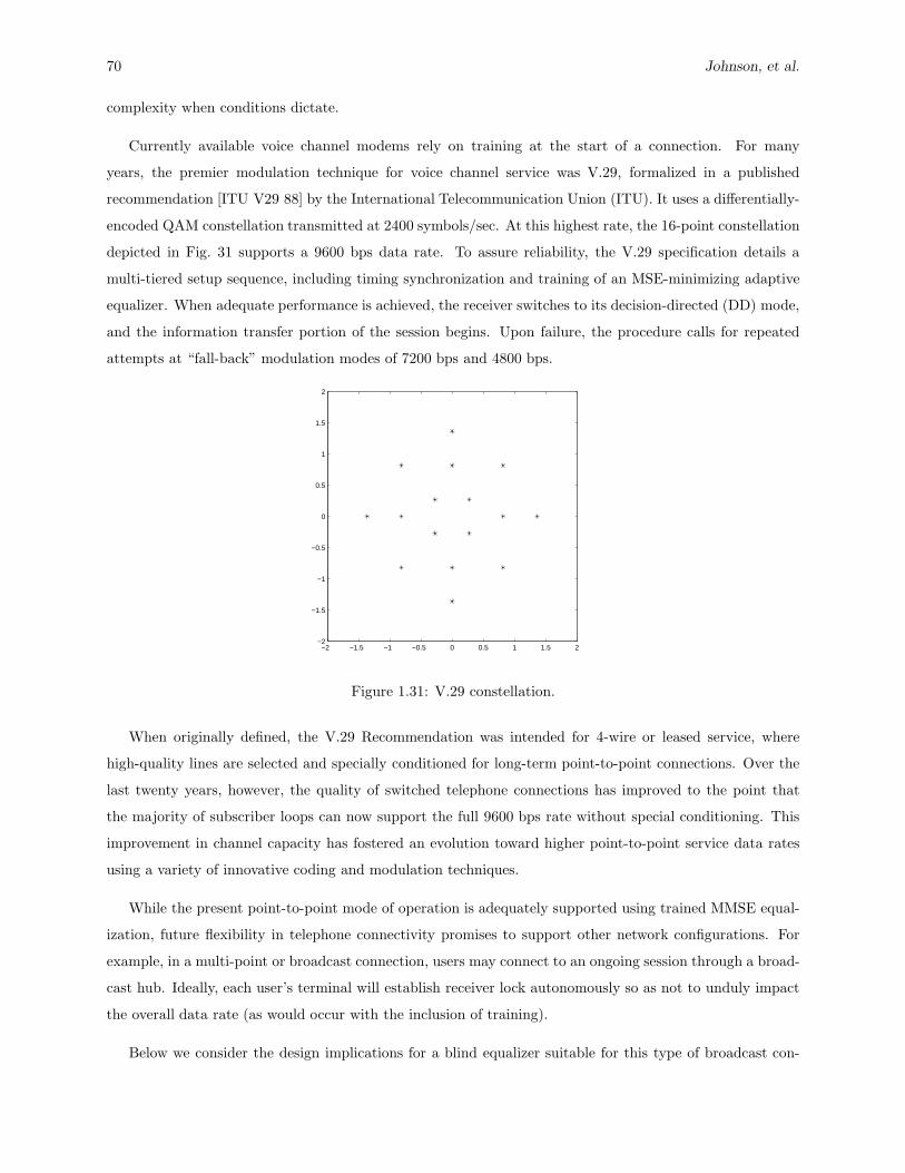
70 Johnson, et al.
complexity when conditions dictate.
Currently available voice channel modems rely on training at the start of a connection. For many
years, the premier modulation technique for voice channel service was V.29, formalized in a published
recommendation [ITU V29 88] by the International Telecommunication Union (ITU). It uses a differentially-
encoded QAM constellation transmitted at 2400 symbols/sec. At this highest rate, the 16-point constellation
depicted in Fig. 31 supports a 9600 bps data rate. To assure reliability, the V.29 specification details a
multi-tiered setup sequence, including timing synchronization and training of an MSE-minimizing adaptive
equalizer. When adequate performance is achieved, the receiver switches to its decision-directed (DD) mode,
and the information transfer portion of the session begins. Upon failure, the procedure calls for repeated
attempts at “fall-back” modulation modes of 7200 bps and 4800 bps.
−2 −1.5 −1 −0.5 0 0.5 1 1.5 2−2
−1.5
−1
−0.5
0
0.5
1
1.5
2
Figure 1.31: V.29 constellation.
When originally defined, the V.29 Recommendation was intended for 4-wire or leased service, where
high-quality lines are selected and specially conditioned for long-term point-to-point connections. Over the
last twenty years, however, the quality of switched telephone connections has improved to the point that
the majority of subscriber loops can now support the full 9600 bps rate without special conditioning. This
improvement in channel capacity has fostered an evolution toward higher point-to-point service data rates
using a variety of innovative coding and modulation techniques.
While the present point-to-point mode of operation is adequately supported using trained MMSE equal-
ization, future flexibility in telephone connectivity promises to support other network configurations. For
example, in a multi-point or broadcast connection, users may connect to an ongoing session through a broad-
cast hub. Ideally, each user’s terminal will establish receiver lock autonomously so as not to unduly impact
the overall data rate (as would occur with the inclusion of training).
Below we consider the design implications for a blind equalizer suitable for this type of broadcast con-

The Core of FSE-CMA Behavior Theory 71
nection over existing telephone transmission facilities. The goal for such a blind equalizer is to reduce
constellation dispersion to the point where a decision-directed scheme can reliably converge to the MMSE
equalizer solution. Note that, while we illustrate using the V.29 modulation format, this by no means
represents a limit on the data rate.
The typical voice channel has the frequency response magnitude shown in Fig. 30(a) and has the impulse
response magnitude seen in Fig. 30(b), where the bulk of the energy is confined to a time duration on
the order of 2-3 ms. For our design, we recall the equalizer length discussion in Section 10.4 and select
an equalizer duration of 30 T/2-spaced taps (spanning 6.25 ms, or about twice the channel spread). For
adequate agility, we specify a step-size µ = 0.001, providing a basic response time in the millisecond range.
The performance of this prototype design can be demonstrated using a record of actual V.29 signal
captured at a subscriber’s premises (as found in the SPIB database). The waveform is quadrature down-
converted by the known carrier frequency of 1700 Hz and sampled at a T/2-spaced rate of 4800 samples/sec.
The resulting complex baseband samples are plotted in Fig. 32, where the indistinct cloud indicates complete
closure of the eye of the data waveform. Following convergence of the blind equalizer, the samples take the
form shown in Fig. 33, clearly exhibiting clustering consistent with the V.29 constellation. At this point,
a phase-tracking loop is used to estimate bulk phase error and properly align the constellation with the
decision regions. Figure 34 shows the end result following switch-over to the decision-directed mode.
−2 −1.5 −1 −0.5 0 0.5 1 1.5 2−2
−1.5
−1
−0.5
0
0.5
1
1.5
2
real
imag
inar
y
Figure 1.32: T/2-spaced input in V.29 demodulation example.
It is interesting to examine Fig. 33, the constellation following blind equalization, more closely. The
elongated shape of the individual cluster points is symptomatic of “phase roll” due to error in the estimation
of carrier frequency. In this case, the accumulated phase change amounts to only about 20◦ over the
observation window. In many cases the carrier offset may be several Hz (e.g., in analog FDM transmission),
resulting in a spinning of the equalizer output constellation, as illustrated in Fig. 35. Because its adaptation
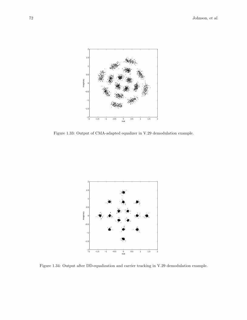
72 Johnson, et al.
−2 −1.5 −1 −0.5 0 0.5 1 1.5 2−2
−1.5
−1
−0.5
0
0.5
1
1.5
2
real
imag
inar
y
Figure 1.33: Output of CMA-adapted equalizer in V.29 demodulation example.
−2 −1.5 −1 −0.5 0 0.5 1 1.5 2−2
−1.5
−1
−0.5
0
0.5
1
1.5
2
real
imag
inar
y
Figure 1.34: Output after DD-equalization and carrier tracking in V.29 demodulation example.

The Core of FSE-CMA Behavior Theory 73
depends only on modulus error, CMA-based blind equalization is largely immune to such phase drift and
frequency error. By decoupling mitigation of channel effects from carrier phase tracking circuitry in this
manner, accurate carrier phase recovery is greatly simplified.
−2 −1.5 −1 −0.5 0 0.5 1 1.5 2−2
−1.5
−1
−0.5
0
0.5
1
1.5
2
real
imag
inar
y
Figure 1.35: Output of CMA-adapted equalizer under 2 Hz of carrier frequency offset in V.29 demodulation
example.
The specifics of this modem design are based on dispersion exhibited by a typical voice channel and
serve as a feasibility baseline for the extension of traditional voice channel technology. The benefits possible
through blind recovery enable modem usage in the broadcast environment of the future.
Digital TV: The Broadband Coaxial Cable Channel
Next, we focus on the use of coaxial cable as a transmission medium for broadcast distribution of digital
television signals for residential coverage. Cable service providers operate regional “head end” distribution
centers, where national and international feeds are combined with local programming into a composite sig-
nal and conditioned for transmission to local subscribers. Much of the physical cable currently in place
was originally intended for analog transmission, that is, 6-MHz TV signals frequency-multiplexed to channel
assignments of up to 700 MHz. Relative to broadcast transmission, distribution via cable provides a po-
tentially higher-quality signal, unaffected by atmospheric attenuation, RF interference and multipath, and
where frequency-dependent losses are normally small throughout any given 6-MHz band. Practical cable
systems, however, do suffer from non-ideal effects related to reflective mismatched terminations, imperfect
isolation, and crosstalk. In addition, shielding breaks or weak connections may allow so-called “ingress”
interference to enter the band (from atmospheric EMI and/or RF broadcast signals).
To provide better signal quality while improving spectral efficiency, digital transmission of TV signals
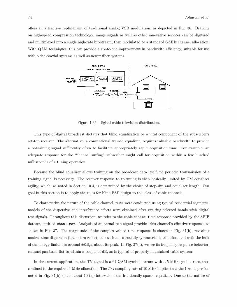
74 Johnson, et al.
offers an attractive replacement of traditional analog VSB modulation, as depicted in Fig. 36. Drawing
on high-speed compression technology, image signals as well as other innovative services can be digitized
and multiplexed into a single high-rate bit-stream, then modulated to a standard 6-MHz channel allocation.
With QAM techniques, this can provide a six-to-one improvement in bandwidth efficiency, suitable for use
with older coaxial systems as well as newer fiber systems.
Figure 1.36: Digital cable television distribution.
This type of digital broadcast dictates that blind equalization be a vital component of the subscriber’s
set-top receiver. The alternative, a conventional trained equalizer, requires valuable bandwidth to provide
a re-training signal sufficiently often to facilitate appropriately rapid acquisition time. For example, an
adequate response for the “channel surfing” subscriber might call for acquisition within a few hundred
milliseconds of a tuning operation.
Because the blind equalizer allows training on the broadcast data itself, no periodic transmission of a
training signal is necessary. The receiver response to re-tuning is then basically limited by CM equalizer
agility, which, as noted in Section 10.4, is determined by the choice of step-size and equalizer length. Our
goal in this section is to apply the rules for blind FSE design to this class of cable channels.
To characterize the nature of the cable channel, tests were conducted using typical residential segments;
models of the dispersive and interference effects were obtained after exciting selected bands with digital
test signals. Throughout this discussion, we refer to the cable channel time response provided by the SPIB
dataset, entitled chan1.mat. Analysis of an actual test signal provides this channel’s effective response, as
shown in Fig. 37. The magnitude of the complex-valued time response is shown in Fig. 37(b), revealing
modest time dispersion (i.e., micro-reflections) with an essentially symmetric distribution, and with the bulk
of the energy limited to around ±0.5µs about its peak. In Fig. 37(a), we see its frequency response behavior:
channel passband flat to within a couple of dB, as is typical of properly maintained cable systems.
In the current application, the TV signal is a 64-QAM symbol stream with a 5-MHz symbol rate, thus
confined to the required 6-MHz allocation. The T/2 sampling rate of 10 MHz implies that the 1 µs dispersion
noted in Fig. 37(b) spans about 10-tap intervals of the fractionally-spaced equalizer. Due to the nature of
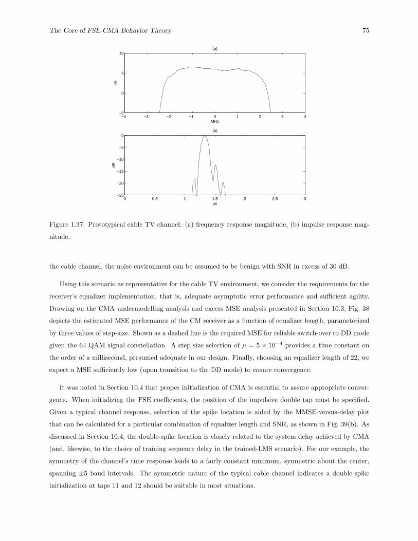
The Core of FSE-CMA Behavior Theory 75
−4 −3 −2 −1 0 1 2 3 4−5
0
5
10(a)
MHzdB
0 0.5 1 1.5 2 2.5 3−25
−20
−15
−10
−5
0
µs
dB
(b)
Figure 1.37: Prototypical cable TV channel: (a) frequency response magnitude, (b) impulse response mag-
nitude.
the cable channel, the noise environment can be assumed to be benign with SNR in excess of 30 dB.
Using this scenario as representative for the cable TV environment, we consider the requirements for the
receiver’s equalizer implementation, that is, adequate asymptotic error performance and sufficient agility.
Drawing on the CMA undermodelling analysis and excess MSE analysis presented in Section 10.3, Fig. 38
depicts the estimated MSE performance of the CM receiver as a function of equalizer length, parameterized
by three values of step-size. Shown as a dashed line is the required MSE for reliable switch-over to DD mode
given the 64-QAM signal constellation. A step-size selection of µ = 5 × 10⁻⁴ provides a time constant on
the order of a millisecond, presumed adequate in our design. Finally, choosing an equalizer length of 22, we
expect a MSE sufficiently low (upon transition to the DD mode) to ensure convergence.
It was noted in Section 10.4 that proper initialization of CMA is essential to assure appropriate conver-
gence. When initializing the FSE coefficients, the position of the impulsive double tap must be specified.
Given a typical channel response, selection of the spike location is aided by the MMSE-versus-delay plot
that can be calculated for a particular combination of equalizer length and SNR, as shown in Fig. 39(b). As
discussed in Section 10.4, the double-spike location is closely related to the system delay achieved by CMA
(and, likewise, to the choice of training sequence delay in the trained-LMS scenario). For our example, the
symmetry of the channel’s time response leads to a fairly constant minimum, symmetric about the center,
spanning ±5 baud intervals. The symmetric nature of the typical cable channel indicates a double-spike
initialization at taps 11 and 12 should be suitable in most situations.
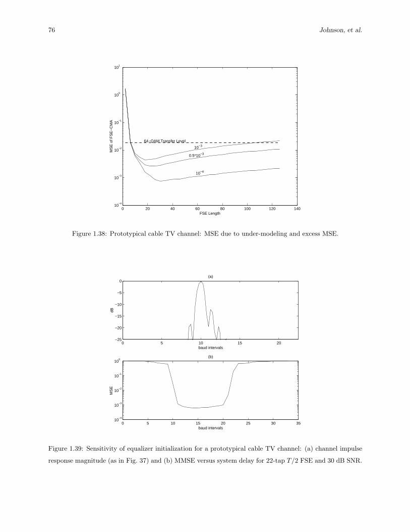
76 Johnson, et al.
0 20 40 60 80 100 120 14010
−4
10−3
10−2
10−1
100
101
FSE Length
MS
E o
f FS
E−
CM
A
10−3
0.5*10−3
10−4
64−QAM Transfer Level
Figure 1.38: Prototypical cable TV channel: MSE due to under-modeling and excess MSE.
0 5 10 15 20−25
−20
−15
−10
−5
0
baud intervals
dB
(a)
0 5 10 15 20 25 30 3510
−4
10−3
10−2
10−1
100
baud intervals
MS
E
(b)
Figure 1.39: Sensitivity of equalizer initialization for a prototypical cable TV channel: (a) channel impulse
response magnitude (as in Fig. 37) and (b) MMSE versus system delay for 22-tap T/2 FSE and 30 dB SNR.

The Core of FSE-CMA Behavior Theory 77
To validate our design choices, Fig. 40 shows an ensemble-averaged MSE trajectory characterizing CMA
adaptation. Ten sequences of 64-QAM symbols were passed through our typical channel model and the result
applied to the CMA-adapted blind FSE. The plot shows transient behavior of the average mean-squared
error, where the acceptable “open-eye” condition necessary for switch-over to DD adaptation occurs in about
a millisecond.
0 0.2 0.4 0.6 0.8 1 1.2 1.4 1.6 1.8 2
x 104
10−3
10−2
10−1
100
T/2 samples
MS
E
Figure 1.40: The MSE trajectory of CMA as applied to the prototypical cable TV channel.
Based on these observations, we can see that reliable blind reception of digital television signals is possible
with reasonably simple and low-cost hardware at the receiver, as is critical for commercial acceptance. Note
that our design approach has been purposely conservative in order to accommodate extremes in channel
behavior that might be encountered in less ideal situations.
Mobile Radio: The Terrestrial Microwave Channel
In recent years, point-to-point microwave transmission, which traditionally used analog frequency modula-
tion, has been aggressively converted to higher efficiency digital modulation techniques. This transition has
been motivated by increased demands for bandwidth, and has been made possible by advances in high-speed
processing technology over the last decade. A traditional point-to-point link deployment involves fixed an-
tenna installations with narrow collinear beams, carefully adjusted to minimize reflective interference. This
type of system has traditionally served the needs of remote long-haul telephone service as well as intra-urban
private voice, video, and data feeds. In this section we consider equalization requirements for digital radio
service involving a terrestrial channel.
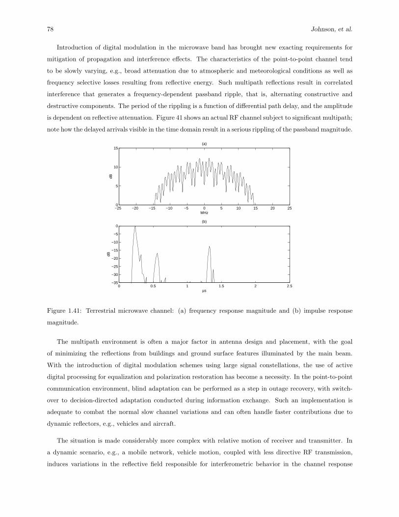
78 Johnson, et al.
Introduction of digital modulation in the microwave band has brought new exacting requirements for
mitigation of propagation and interference effects. The characteristics of the point-to-point channel tend
to be slowly varying, e.g., broad attenuation due to atmospheric and meteorological conditions as well as
frequency selective losses resulting from reflective energy. Such multipath reflections result in correlated
interference that generates a frequency-dependent passband ripple, that is, alternating constructive and
destructive components. The period of the rippling is a function of differential path delay, and the amplitude
is dependent on reflective attenuation. Figure 41 shows an actual RF channel subject to significant multipath;
note how the delayed arrivals visible in the time domain result in a serious rippling of the passband magnitude.
−25 −20 −15 −10 −5 0 5 10 15 20 250
5
10
15(a)
MHz
dB
0 0.5 1 1.5 2 2.5−35
−30
−25
−20
−15
−10
−5
0
µs
dB
(b)
Figure 1.41: Terrestrial microwave channel: (a) frequency response magnitude and (b) impulse response
magnitude.
The multipath environment is often a major factor in antenna design and placement, with the goal
of minimizing the reflections from buildings and ground surface features illuminated by the main beam.
With the introduction of digital modulation schemes using large signal constellations, the use of active
digital processing for equalization and polarization restoration has become a necessity. In the point-to-point
communication environment, blind adaptation can be performed as a step in outage recovery, with switch-
over to decision-directed adaptation conducted during information exchange. Such an implementation is
adequate to combat the normal slow channel variations and can often handle faster contributions due to
dynamic reflectors, e.g., vehicles and aircraft.
The situation is made considerably more complex with relative motion of receiver and transmitter. In
a dynamic scenario, e.g., a mobile network, vehicle motion, coupled with less directive RF transmission,
induces variations in the reflective field responsible for interferometric behavior in the channel response

The Core of FSE-CMA Behavior Theory 79
(i.e., an in-band “wobbling” fade). This is further complicated by other distributed and motion-induced
reflections, e.g., water motion or shimmering foliage. These features call for significant improvement in
receiver tracking ability in order to adequately mitigate inter-symbol interference. Furthermore, the nature
of the mobile networked environment precludes extensive training. Instead, for the multi-point configuration,
it is far preferable that blind adaptation be used to adjust equalizer coefficients, in order to avoid suspension
of productive transmission to other receivers in the network.
For this design case we focus on one example of a channel seen by a moving receiver, that is, one node
of a networked configuration. The nature of the expected channel then determines the design parameters
of the blind equalizer. Specifically, we consider a channel measured as part of an RF survey study Applied
Signal Technology conducted in 1996 in rural Northern California [Behm ASIL 97]. A sample dataset from
this survey is available from the SPIB database, entitled hillshadow.otm.4GHz.snp. Snapshots of a digital
transmission at 25 Msymbol/s, down-converted to IF from 4.5 GHz, were taken from a vehicle traveling at
modest speed in the vicinity of a fixed transmitter site. By analyzing snapshots taken at 200 ms intervals,
the channel characteristics can be estimated using the blind recovery technique of [Gooch ICC 88] and the
nature of their variation determined. Figure 42 shows that time-variations in the multipath field can be
significant, with radical differences exhibited in the impulse response.
10 20 30 40 50 60 70 80 90 1000
0.5
1
snap
7
10 20 30 40 50 60 70 80 90 1000
0.5
1
snap
8
10 20 30 40 50 60 70 80 90 1000
0.5
1
snap
9
10 20 30 40 50 60 70 80 90 1000
0.5
1
snap
10
T/2 spaced chan coef
Figure 1.42: Mobile microwave: estimates of channel impulse responses derived from data records separated
by 200 ms intervals.
This case represents conflicting design goals: the channel delay spread exhibited in Fig. 41(b), typically
spanning 10 to 25 symbols (400 to 1000 ns), calls for a relatively long equalizer for adequate ISI recovery,
and thus to maintain suitable steady-state performance, the step-size must be kept small. However, the

80 Johnson, et al.
time-varying nature of the mobile channel requires a step-size large enough to track the typical multipath
variations exhibited by Fig. 42.
In Sidebar C of [Treichler SPM 96], the minimum recommended T/2-spaced equalizer length for the
QPSK source used here is 2 taps for each symbol period of delay spread. With a noted maximum delay
spread of approximately 25 symbols, and using an additional factor-of-two margin-of-safety, we choose 100
equalizer taps.
From Sidebar D of [Treichler SPM 96], with a unit-variance received signal and an equalizer of up to 100
taps, the recommended upper bound on the step-size (of LMS22) is 2 divided by the number of taps, that
is, 0.02 in our design. The minimum step-size is related to the variability of the channels of interest. For
example, Fig. 42 exhibits substantial variation every 200 ms. Presuming that we wish to have a convergence
time constant less than 100 times this 0.2 second interval, the average time constant formula for LMS suggests
(as discussed in Sidebar D of [Treichler SPM 96]) that for a T/2-spaced FSE,
µ >1
(# of taps) · (# of baud intervals per second) · (minimum convergence time constant).
For 25 Mbaud/sec and 100 equalizer taps, this implies that µ should be chosen greater than 2×10⁻⁵. Hence,
we choose µ = 10−3.
Our choices of length and step-size allowed us to equalize and accurately demodulate the QPSK signal
corresponding to the channel shown in Fig. 42. This is demonstrated by the equalized constellation in Fig. 43
for the source constellation of Fig. 44.
This discussion has illustrated use of blind techniques for digital transmission over three very differ-
ent channels. In each case, the motivation is blind adaptation of the equalizer to avoid disruption of the
transmitter’s information transfer. And in each case, once adjustment is sufficient to restore constellation
integrity, the conventional decision-directed mode is begun. One should note that, for each scenario, future
applications involving more elaborate network topologies hinge on the success of blind equalization.
22In our application of LMS step-size and length selection guidelines to CMA, we exploit the similarities between LMS
and CMA convergence behavior discussed in Section 10.4 (and more technically in Section 10.3). Though CMA and LMS
convergence rates may differ by a factor of two or so, we regard such differences to be subsumed by our wide safety margins.
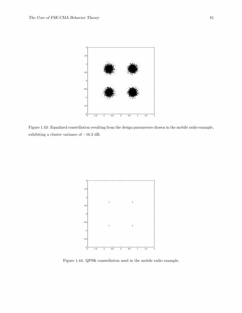
The Core of FSE-CMA Behavior Theory 81
−2 −1.5 −1 −0.5 0 0.5 1 1.5 2−2
−1.5
−1
−0.5
0
0.5
1
1.5
2
Figure 1.43: Equalized constellation resulting from the design parameters chosen in the mobile radio example,
exhibiting a cluster variance of −16.3 dB.
−2 −1.5 −1 −0.5 0 0.5 1 1.5 2−2
−1.5
−1
−0.5
0
0.5
1
1.5
2
Figure 1.44: QPSK constellation used in the mobile radio example.

82 Johnson, et al.
1.6 Conclusions
The most basic of adaptive filter configurations in practice and pedagogy is a tapped-delay-line with impulse
response coefficients updated via the LMS algorithm in the presence of a replica of the desired filter output
sequence (e.g., a training sequence). Thirty years of experience have taught us how to use LMS even though
the theory describing its behavior in all pragmatic circumstances is still not complete. We are in an earlier
period in a similar pattern of growing utilization and understanding of the constant modulus algorithm
(CMA), which has proven to be the baseline algorithm for a variety of applications where the replica of the
desired filter output is unavailable, that is, the blind scenario.
The movement from point-to-point, session-oriented communications, for which cooperative equalizer
training was acceptable, to digital multi-point and broadcast systems, for which training is unacceptable,
mandates blind equalization. Because CMA is the one blind algorithm for adaptive equalization that has
seen widespread success in operational communication systems, we have assembled a set of design guidelines
for it in this book chapter.
The basic pedagogy employed in this chapter for organizing a behavior theory for a blind fractionally-
spaced equalizer is similar to that used in a variety of widely cited textbooks for describing trained, baud-
spaced equalizer behavior theory. This approach is bolstered by recent results—described in previous sections
of this book chapter—on the similarity of CM and MSE cost function minima. This prompts the adoption
of the taxonomy associated with LMS-adapted equalizer design rules. Indeed, the content of this chapter
can be characterized in these terms:
• Establish (in Sections 10.2 and 10.3) a relationship between the CM-cost minimizing receiver and the
MSE minimizing receiver, and therefore between their respective stochastic gradient descent schemes
CMA and LMS.
• Collect (in Section 10.3) current understanding of effects of frequency-selective propagation channel
response characteristics, source sequence properties, and relative level of additive noise on appropriate
adaptive filter length, CMA step-size, and coefficient initialization.
• Extract and illustrate design guidelines with academic examples (in Section 10.4) and case studies (in
Section 10.5).
This book chapter, as a chronicle of the current state-of-the-art in converting an understanding of the
behavior of CMA into useful design guidelines, indicates that there is still much more to do, both in terms
of fundamental advances in understanding and in terms of a variety of specific details. However, we believe
that this chapter—and the almost 20 years of engineering development, practice and basic research in blind
equalization via CMA upon which this chapter is based—also establishes CMA as ready for prime time.

Bibliography
[AST Report 96] C. Prettie, R. Yu, J. Trollman, J. Shabel, V. Procopio, and K. Wong, Results of Laboratory
and Field Measurements of Propagation Effects for On-The-Move High Capacity Trunk Radio, Scientific
and Technical Report B001, Applied Signal Technology, Inc., Sunnyvale, CA, Nov. 1996.
[Axford TSP 98] R.A. Axford, Jr., L.B. Milstein, and J.R. Zeidler, “The effects on PN sequences on the
misconvergence of the constant modulus algorithm,” IEEE Transactions on Signal Processing, vol. 46,
no. 2, pp. 519-23, Feb. 1998.
[Behm ASIL 97] J.D. Behm, T.J. Endres, P. Schniter, C.R. Johnson, Jr., C. Prettie, M.L. Alberi, and
I. Fijalkow, “Characterization of an empirically-derived database of time-varying microwave channel
responses,” in Proc. Asilomar Conference on Signals, Systems and Computers (Pacific Grove, CA), pp.
1549-53, 2-5 Nov. 1997.
[Bellini (Haykin) 94] S. Bellini, “Bussgang techniques for blind deconvolution and equalization,” in Blind
Deconvolution, ed. S. Haykin, Englewood Cliffs, NJ: Prentice-Hall, 1994, pp. 60-120.
[Benveniste Book 90] A. Benveniste, M. M’etivier, and P. Priouret, Adaptive Algorithms and Stochastic
Approximations, Paris, France: Springer-Verlag, 1990.
[Bussgang MIT 52] J.J. Bussgang, Crosscorrelation Functions of Amplitude-Distorted Gaussian Signals,
Technical Report 216, MIT Research Laboratory of Electronics, Cambridge, MA, 1952.
[Caines Book 88] P.E. Caines, Linear Stochastic Systems, New York, NY: John Wiley & Sons, Inc., 1988.
[Casas DSP 97] R.A. Casas, F. Lopez de Victoria, I. Fijalkow, P. Schniter, T.J. Endres, and C.R. Johnson,
Jr., “On MMSE fractionally-spaced equalizer design,” in Proc. International Conference on Digital
Signal Processing (Santorini, Greece), pp. 395-8, 2-4 July 1997.
[Cioffi TCOM 95] J.M. Cioffi, G.P. Dudevoir, M.V. Eyuboglu, and G.D. Forney, Jr., “MMSE decision feed-
back equalization and coding – Part I and II,” IEEE Transactions on Communications, vol. 43, no. 10,
pp. 2582-604, Oct. 1995.
83
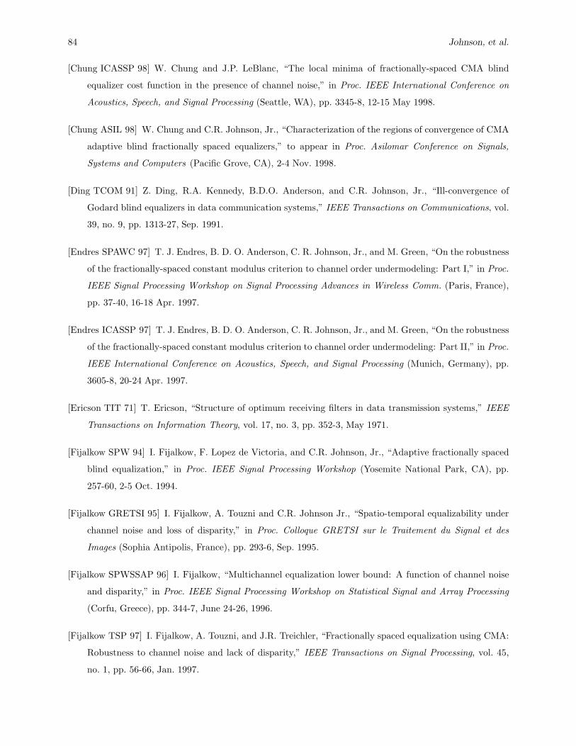
84 Johnson, et al.
[Chung ICASSP 98] W. Chung and J.P. LeBlanc, “The local minima of fractionally-spaced CMA blind
equalizer cost function in the presence of channel noise,” in Proc. IEEE International Conference on
Acoustics, Speech, and Signal Processing (Seattle, WA), pp. 3345-8, 12-15 May 1998.
[Chung ASIL 98] W. Chung and C.R. Johnson, Jr., “Characterization of the regions of convergence of CMA
adaptive blind fractionally spaced equalizers,” to appear in Proc. Asilomar Conference on Signals,
Systems and Computers (Pacific Grove, CA), 2-4 Nov. 1998.
[Ding TCOM 91] Z. Ding, R.A. Kennedy, B.D.O. Anderson, and C.R. Johnson, Jr., “Ill-convergence of
Godard blind equalizers in data communication systems,” IEEE Transactions on Communications, vol.
39, no. 9, pp. 1313-27, Sep. 1991.
[Endres SPAWC 97] T. J. Endres, B. D. O. Anderson, C. R. Johnson, Jr., and M. Green, “On the robustness
of the fractionally-spaced constant modulus criterion to channel order undermodeling: Part I,” in Proc.
IEEE Signal Processing Workshop on Signal Processing Advances in Wireless Comm. (Paris, France),
pp. 37-40, 16-18 Apr. 1997.
[Endres ICASSP 97] T. J. Endres, B. D. O. Anderson, C. R. Johnson, Jr., and M. Green, “On the robustness
of the fractionally-spaced constant modulus criterion to channel order undermodeling: Part II,” in Proc.
IEEE International Conference on Acoustics, Speech, and Signal Processing (Munich, Germany), pp.
3605-8, 20-24 Apr. 1997.
[Ericson TIT 71] T. Ericson, “Structure of optimum receiving filters in data transmission systems,” IEEE
Transactions on Information Theory, vol. 17, no. 3, pp. 352-3, May 1971.
[Fijalkow SPW 94] I. Fijalkow, F. Lopez de Victoria, and C.R. Johnson, Jr., “Adaptive fractionally spaced
blind equalization,” in Proc. IEEE Signal Processing Workshop (Yosemite National Park, CA), pp.
257-60, 2-5 Oct. 1994.
[Fijalkow GRETSI 95] I. Fijalkow, A. Touzni and C.R. Johnson Jr., “Spatio-temporal equalizability under
channel noise and loss of disparity,” in Proc. Colloque GRETSI sur le Traitement du Signal et des
Images (Sophia Antipolis, France), pp. 293-6, Sep. 1995.
[Fijalkow SPWSSAP 96] I. Fijalkow, “Multichannel equalization lower bound: A function of channel noise
and disparity,” in Proc. IEEE Signal Processing Workshop on Statistical Signal and Array Processing
(Corfu, Greece), pp. 344-7, June 24-26, 1996.
[Fijalkow TSP 97] I. Fijalkow, A. Touzni, and J.R. Treichler, “Fractionally spaced equalization using CMA:
Robustness to channel noise and lack of disparity,” IEEE Transactions on Signal Processing, vol. 45,
no. 1, pp. 56-66, Jan. 1997.
The Core of FSE-CMA Behavior Theory 85
[Fijalkow TSP 98] I. Fijalkow, C. Manlove, and C.R. Johnson, Jr., “Adaptive fractionally spaced blind CMA
equalization: Excess MSE,” IEEE Transactions on Signal Processing, vol. 46, no. 1, pp. 227-31, Jan.
1998.
[Foschini ATT 85] G.J. Foschini, “Equalizing without altering or detecting data (digital radio systems),”
AT&T Technical Journal, vol. 64, no. 8, pp. 1885-911, Oct. 1985.
[Fuhrmann Book 96] P.A. Fuhrmann, A Polynomial Approach to Linear Algebra, New York, NY: Springer-
Verlag, 1996.
[Gitlin Book 92] R.D. Gitlin, J.F. Hayes, and S.B. Weinstein, Data Communications Principles, New York,
NY: Plenum Press, 1992.
[Godard TCOM 80] D.N. Godard, “Self-recovering equalization and carrier tracking in two-dimensional data
communication systems,” IEEE Transactions on Communications, vol. 28, no. 11, pp. 1867-75, Nov.
1980.
[Gooch ICC 88] R.P. Gooch and J.C. Harp, “Blind channel identification using the constant modulus adap-
tive algorithm,” in Proc. IEEE International Conference on Communications (Philadelphia, PA), pp.
75-9, June 12-15, 1988.
[Gray TIT 72] R.M. Gray, “On the asymptotic eigenvalue distribution of Toeplitz matrices,” IEEE Trans-
actions on Information Theory, vol. 23, pp. 357-68, Nov. 1980.
[Gu CISS 98] M. Gu and L. Tong, “Geometrical characterizations of constant modulus receivers,” to appear
in Proc. Conference on Information Science and Systems (Princeton, NJ), Mar. 1998.
[Haykin Book 94] S. Haykin (Editor), Blind Deconvolution, Englewood Cliffs, NJ: Prentice-Hall, 1994.
[Haykin Book 96] S. Haykin, Adaptive Filter Theory, 3rd ed., Englewood Cliffs, NJ: Prentice-Hall, 1996.
[ITU V29 88] International Telecommunication Union, Data communication over the telephone network:
9600 bits per second modem standardized for use on point-to-point 4-wire leased telephone-type circuits,
ITU-T Recommendation V.29, Blue Book, vol. VIII.I, Geneva, Switzerland, 1988.
[Johnson IJACSP 95] C.R. Johnson, Jr. and B.D.O. Anderson, “Godard blind equalizer error surface char-
acteristics: White, zero-mean, binary case,” International Journal of Adaptive Control & Signal Pro-
cessing, vol. 9, pp. 301-24, July-Aug. 1995.
[Johnson PROC 98] C.R. Johnson, Jr., P. Schniter, T.J. Endres, J.D. Behm, D.R. Brown, and R.A. Casas,
“Blind equalization using the constant modulus criterion: A review,” Proceedings of the IEEE special
issue on Blind System Identification and Estimation, vol. 86, no. 10, pp. 1927-50, Oct. 1998.
[Kailath Book 80] T. Kailath, Linear Systems, Englewood Cliffs, NJ: Prentice-Hall, 1980.
86 Johnson, et al.
[Lambotharan SP 97] S. Lambotharan, J. Chambers, and C.R. Johnson, Jr., “Attraction of saddles and slow
convergence in CMA adaptation,” Signal Processing, vol. 59, no. 2, pp. 335-40, June 1997.
[Larimore ICASSP 83] M.G. Larimore and J.R. Treichler, “Convergence behavior of the constant modu-
lus algorithm,” in Proc. IEEE International Conference on Acoustics, Speech, and Signal Processing
(Boston, MA), pp. 13-16, 14-16 Apr. 1983.
[Larimore ICASSP 97] M.G. Larimore, S.L. Wood, and J.R. Treichler, “Performance costs for theoretical
minimum-length equalizers,” in Proc. IEEE International Conference on Acoustics, Speech, and Signal
Processing (Munich, Germany), pp. 2477-80, 21-24 Apr. 1997.
[LeBlanc Thesis 95] J.P. LeBlanc, “Effects of source distributions and correlation on fractionally spaced
blind constant modulus algorithm equalizers,” Ph.D. dissertation, Cornell University, Ithaca, NY, Aug.
1995.
[LeBlanc ICASSP 96] J.P. LeBlanc, I. Fijalkow, and C.R. Johnson Jr., “Fractionally-spaced constant mod-
ulus algorithm blind equalizer error surface characterization: Effects of source distributions,” in Proc.
IEEE International Conference on Acoustics, Speech, and Signal Processing (Atlanta, GA), pp. 2944-7,
7-9 May 1996.
[LeBlanc IJACSP 98] J.P. LeBlanc, I. Fijalkow, and C.R. Johnson, Jr., “CMA fractionally spaced equalizers:
Stationary points and stability under IID and temporally correlated sources,” International Journal of
Adaptive Control & Signal Processing, vol. 12, no. 2, pp. 135-55, Mar. 1998.
[Lee Book 94] E.A. Lee and D.G. Messerschmitt, Digital Communication, 2nd ed., Boston, MA: Kluwer
Academic Publishers, 1994.
[Li TSP 95] Y. Li and Z. Ding, “Convergence analysis of finite length blind adaptive equalizers,” IEEE
Transactions on Signal Processing, vol. 43, no. 9, pp. 2120-9, Sep. 1995.
[Li TSP 96a] Y. Li and Z. Ding, “Global convergence of fractionally spaced Godard (CMA) adaptive equal-
izers,” IEEE Transactions on Signal Processing, vol. 44, no. 4, pp. 818-26, Apr. 1996.
[Li TSP 96b] Y. Li, K.J.R. Liu, and Z. Ding, “Length and cost dependent local minima of unconstrained
blind channel equalizers,” IEEE Transactions on Signal Processing, vol. 44, no. 11, pp. 2726-35, Nov.
1996.
[Li TSP 96c] Y. Li and K.J.R. Liu, “Static and dynamic convergence behavior of adaptive blind equalizers,”
IEEE Transactions on Signal Processing, vol. 44, no. 11, pp. 2736-45, Nov. 1996.
[Liu PROC 98] R.W. Liu, editor, Proceedings of the IEEE: Special Issue on Blind System Identification and
Estimation, Piscataway, NJ: Institute of Electrical and Electronic Engineers, vol. 86, no. 10, Oct. 1998.
The Core of FSE-CMA Behavior Theory 87
[Ljung Book 83] L. Ljung and T. Soderstrom, Theory and Practice of Recursive Identification, Cambridge,
MA: M.I.T. Press, 1983.
[Lucky BSTJ 66] R.W. Lucky, “Techniques for adaptive equalization of digital communication systems,”
Bell System Technical Journal, vol. 45, pp. 255-86, Feb. 1966.
[Luenberger Book 90] D.G. Luenberger, Optimization by Vector Space Methods, 2nd ed., New York, NY:
Wiley, 1990.
[Macchi Book 95] O. Macchi, Adaptive Processing: The Least Mean Squares Approach with Applications in
Transmission, Chichester, NY: Wiley, 1995.
[Moulines TSP 95] E. Moulines, P. Duhamel, J. Cardoso, and S. Mayrargue, “Subspace methods for blind
identification of multichannel FIR filters,” IEEE Transactions on Signal Processing, vol. 43, no. 2, pp.
516-25, Feb. 1995.
[Papadias ICASSP 97] C.B. Papadias, “On the existence of undesired global minima of Godard equaliz-
ers,” in Proc. IEEE International Conference on Acoustics, Speech, and Signal Processing (Munich,
Germany), pp. 3937-40, 20-24 Apr. 1997.
[Paulraj SPM 97] A.J. Paulraj and C.B. Papadias, “Space-time processing for wireless communications,”
IEEE Signal Processing Magazine, vol. 14, no. 6, pp. 49-83, Nov. 1997.
[Proakis Book 95] J.G. Proakis, Digital Communications, 3rd ed., New York, NY: McGraw-Hill, 1995.
[Qureshi PROC 85] S.U.H. Qureshi, “Adaptive equalization,” Proceedings of the IEEE, vol. 73, no. 9, pp.
1349-87, Sep. 1985.
[Rosenblatt Book 85] M. Rosenblatt, Stationary Sequences and Random Fields, Boston, MA: Birkhauser,
1985.
[Strang Book 88] G. Strang, Linear Algebra and its Applications, 3rd ed., Fort Worth, TX: Harcourt Brace
Jovanovich, 1988.
[Tong TIT 95] L. Tong, G. Xu, B. Hassibi, and T. Kailath, “Blind identification and equalization based
on second-order statistics: A frequency-domain approach,” IEEE Transactions on Information Theory,
vol. 41, no. 1, pp. 329-34, Jan. 1995.
[Tong SPL 97] L. Tong and H. Zeng, “Channel surfing re-initialization for the constant modulus algorithm,”
IEEE Signal Processing Letters, vol. 4, no. 3, pp. 85-7, Mar. 1997.
[Touzni EUSIPCO 96] A. Touzni and I. Fijalkow, “Does fractionally-spaced CMA converge faster than
LMS?,” in Proc. European Signal Processing Conference (Trieste, Italy), pp. 1227-30, Sep. 1996.

88 Johnson, et al.
[Treichler TASSP 83] J.R. Treichler and B.G. Agee, “A new approach to multipath correction of constant
modulus signals,” IEEE Transactions on Acoustics, Speech, and Signal Processing, vol. ASSP-31, no. 2,
pp. 459-72, Apr. 1983.
[Treichler SPM 96] J.R. Treichler, I. Fijalkow, and C.R. Johnson, Jr., “Fractionally-spaced equalizers: How
long should they really be?,” IEEE Signal Processing Magazine, vol. 13, no. 3, pp. 65-81, May 1996.
[Treichler PROC 98] J.R. Treichler, M.G. Larimore, and J.C. Harp, “Practical blind demodulators for high-
order QAM signals,” Proceedings of the IEEEspecial issue on Blind System Identification and Estima-
tion, vol. 86, no. 10, pp. 1907-26, Oct. 1998.
[Ungerboeck TCOM 76] G. Ungerboeck, “Fractional tap-spacing equalizer and consequences for clock re-
covery in data modems,” IEEE Transactions on Communications, vol. 24, no. 8, pp. 856-64, Aug.
1976.
[Widrow PROC 76] B. Widrow, J.M. McCool, M.G. Larimore and C.R. Johnson, Jr., “Stationary and non-
stationary learning characteristics of the LMS adaptive filter,” Proceedings of the IEEE, vol. 64, no. 8,
pp. 1151-62, Aug. 1976.
[Widrow Book 85] B. Widrow and S.D. Stearns, Adaptive Signal Processing, Englewood Cliffs, NJ: Prentice
Hall, Inc., 1985.
[Zeng ASIL 96] H.H. Zeng, L. Tong and C.R. Johnson, Jr., “Behavior of fractionally-spaced constant mod-
ulus algorithm: Mean square error, robustness and local minima,” in Proc. Asilomar Conference on
Signals, Systems and Computers (Pacific Grove, CA), pp. 305-9, Nov. 1996.
[Zeng TIT 98] H.H. Zeng, L. Tong and C.R. Johnson, Jr., “Relationships between the constant modulus and
Wiener receivers,” IEEE Transactions on Information Theory, vol. 44, no. 4, pp. 1523-38, July 1998.
[Zeng ICC 96] S. Zeng, H.H. Zeng, and L. Tong, “Blind equalization using CMA: Performance analysis and a
new algorithm,” in Proc. IEEE International Conference on Communications (Dallas, TX), pp. 847-51,
June 1996.
Index
Bezout equation, 18
Bussgang, 29
Channel, 12
coaxial cable, 73–77
common subchannel roots, 18, 19
cursor of, 57
folded spectrum, 21
matrix, 15, 18
mobile microwave, 77–80
multichannel model, 13–14
multirate model, 12–13
terrestrial microwave, 57
voiceband modem, 68–73
Constant modulus (CM) criterion, 28–48
cost expression, 29, 30
cost surface, 31–38
effects of channel undermodelling on, 35–36,
41, 57
effects of noise on, 32–34, 40–41
effects of source correlation on, 36
effects of source kurtosis on, 36–38, 54
exact analysis, 41–48
local minima, 34, 42
MSE bound, 48
power constraint, 43
region of attraction, 57
robustness, 39–41
saddle points, 61
signal space property, 43
stationary points, 38–39
Constant Modulus Algorithm (CMA), 48–67
convergence rate of, 49–51, 64
dispersion constant, 48
effects of equalizer length on, 59, 65–66
excess CM-cost, 51
excess MSE, 51–55
initialization of, 56–63
ODE analysis, 49
single-spike initialization, 59
step-size, 50, 63–64
transfer level to decision direction, 66–67
Equalization
and carrier synchronization, 29
blind adaptive linear, 2
fractionally-spaced (FSE), 14
MMSE-FIR, 17, 22–24
MMSE-IIR, 20–21
Wiener, 19
zero-forcing (ZF), 17–19
Godard’s conjecture, 28
Inter-symbol interference (ISI), 17
Kurtosis (normalized), 31
LMS, 24–27
convergence, 26
decision-directed, 28
EMSE, 26
step-size, 27, 80
89

90 Johnson, et al.
Matrix Inversion Lemma, 21
Mean-squared error (MSE), 17
Noise gain, 17, 23
Perfect blind equalization, 30
Perfect symbol recovery (PSR), 17
Receiver, 17
SPIB database, 41, 57, 68
Strong perfect equalization (SPE), 17
System delay, 17, 24, 56, 61
System impulse response, 15, 32
UMSE, 20, 45
V.29 Recommendation, 70