PNWD-3283 WTP-RPT- 070 Rev. 0

The Corrosion Effects of Mercury and Mercury Compounds on WTP Materials: Electrochemical Tests C. F. Windisch, Jr. M. R. Elmore S. G. Pitman E. O. Vela D. R. Weier March 2003 Prepared for Bechtel National, Inc. under Contract 24590-101-TSA-W0000-0004

WTP Project Report

LEGAL NOTICE This report was prepared by Battelle Memorial Institute (Battelle) as an account of sponsored research activities. Neither Client nor Battelle nor any person acting on behalf of either: MAKES ANY WARRANTY OR REPRESENTATION, EXPRESS OR IMPLIED, with respect to the accuracy, completeness, or usefulness of the information contained in this report, or that the use of any information, apparatus, process, or composition disclosed in this report may not infringe privately owned rights; or Assumes any liabilities with respect to the use of, or for damages resulting from the use of, any information, apparatus, process, or composition disclosed in this report. References herein to any specific commercial product, process, or service by trade name, trademark, manufacturer, or otherwise, does not necessarily constitute or imply its endorsement, recommendation, or favoring by Battelle. The views and opinions of authors expressed herein do not necessarily state or reflect those of Battelle.

PNWD-3283 WTP-RPT- 070 Rev. 0

The Corrosion Effects of Mercury and Mercury Compounds on WTP Materials: Electrochemical Tests C. F. Windisch, Jr. M. R. Elmore S. G. Pitman E. O. Vela D. R. Weier

March 2003 Test Specification: 24590-WTP-TSP-RT-01-026 Rev. 0 Test Plan: TP-RPP-WTP-154 Rev. 0 Test Exceptions: None R&T Focus Area: Pretreatment Test Scoping Statement(s): B-83 Battelle—Pacific Northwest Division Richland, Washington 99352

COMPLETENESS OF TESTING

This report describes the results of work and testing specified by Test Specification 24590-WTP-TSP-RT-01-026 Rev. 0 and Test Plan TP-RPP-WTP-154 Rev. 0. The work and any associated testing followed the quality assurance requirements outlined in the Test Specification/Plan. The descriptions provided in this test report are an accurate account of both the conduct of the work and the data collected. Test plan results are reported. Also reported are any unusual or anomalous occurrences that are different from expected results. The test results and this report have been reviewed and verified.

Approved: _____________________________________ _________________ Gordon H. Beeman, Manager Date WTP R&T Support Project

iii

Summary This report summarizes work performed in support of the River Protection Project, Hanford Waste Treatment Plant (RPP-WTP) in accordance with Test Specification 24590-WTP-TSP-RT-01-026 Rev. 0 and Test Plan TP-RPP-WTP-154 Rev. 0, as part of Scoping Statement B-83, which is included in Appendix C of the Research and Technology Plan (BNI 2002).(a) The work discussed here consisted of electrochemical corrosion testing of candidate materials of construction for process equipment and piping that may be exposed to mercury (Hg)-containing waste solutions/process solutions in the plant. The tests conducted for this study were screening tests for follow-on long-term immersion testing, and were designed to 1) eliminate unsuitable alloys from further consideration, and 2) identify appropriate test parameters and their ranges for long-term immersion testing. The alloys tested included 304L stainless steel (SS), 316L SS, 6% Mo (254 SMO), Hastelloy C-22, and Ti Grade 2. The planned test conditions included temperatures of 20°C, 40°C, and 60°C; pH of 0, 1, 3, and 5; and Hg concentrations of 0, 0.0001, 0.001, and 0.01 M. A stock solution with the following composition was used to prepare the individual test solutions (representing the waste/process solutions): 0.1 M Cl-, 0.1 M F-, 0.1 M NO3

-, 0.1 M PO43-, 0.1 M SO4

2-, and 0.1 M Citrate-. During initial testing, the Ti Grade 2 specimens exhibited unacceptably high corrosion rates, even without Hg present, and consequently were not tested further. Due to the apparent buffering nature of the test solutions at these compositions, the lower pH values could not be achieved. Also during initial testing, difficulties were encountered related to Hg solubility in the test solutions and to Hg adsorbing on the specimens, thereby affecting the potential/current measurements. As a result, the original test matrix was modified, as noted below:

• Hg was added as HgCl2 instead of HgNO3. • pH values studied were changed to 1.5, 3, and 5. • Ti Grade 2 was eliminated from consideration after control tests (no Hg). • Cathodic treatment of electrodes in the presence of Hg was eliminated.

For the remainder of the electrochemical testing, based on the revised matrix, the following parameters were used:

• Open Circuit Measurement. Sample is inserted in the solution and the open circuit or corrosion potential (vs. a saturated calomel electrode, SCE) is measured as a function of time for a period of 1 hour after immersion.

• Cyclic Polarization Curve. Experiments with solutions containing Hg were started from the

open-circuit potential (not below it) and scanned up to 1.5 V (instead of 1.2 V). The scan rate was 1 mV/s. The data were used to calculate an anodic Tafel slope and corrosion current, from which the corrosion rate was calculated. Curves from tests with and without Hg were compared. The only other numerical parameter obtained from the cyclic polarization data was the passive current density just anodic to the open-circuit potential. Estimated uncertainties for both the

(a) Bechtel National, Inc. (BNI). 2002. Research and Technology Plan. 24590-WTP-PL-RT-01-002 Rev. 1,

U.S. Department of Energy, Office of River Protection, Richland, WA.

iv

corrosion rate and passive current density were ±10%, as determined by varying the fitting parameters over reasonable limits.

• Tafel Measurement. Data from the revised Cyclic Polarization Curve procedure were used to

calculate the anodic Tafel slope and corrosion current, from which the corrosion rate was estimated.

After testing, some samples were analyzed by microscopy and surface analysis techniques, including X-ray photoelectron spectroscopy (XPS). Raman spectroscopy was used for chemical analysis of solution precipitate. The results of the corrosion testing conducted on the candidate alloys led to several conclusions and recommendations:

• These screening tests showed that, because of their very low solubility, mercurous (Hg+) salts were unsuitable for the test solutions. (Mercurous nitrate, HgNO3, was the salt originally planned to be used, but further tests showed that the Hg needed to be added as a mercuric, Hg+2, salt. Mercuric chloride, HgCl2, was found to be suitable and was used for the remainder of the corrosion testing.)

• The corrosion rates for the tested alloys (excluding Ti Grade 2) for almost all conditions

(Hg concentration, pH, and temperature) were approximately 1 mil per year (mpy) or less. One experiment for 316L SS gave a somewhat higher value. Of these measurements, most values were on the order of 0.2 mpy or less.

• The principal parameter influencing the corrosion rate was the alloy composition. Averages of all

of the corrosion rates for the same alloys indicated that 316L exhibited the highest corrosion rates, followed by 304L SS, 6% Mo, and Hastelloy C-22. However, the latter three were statistically very similar, with large overlapping uncertainties.

• Increasing Hg concentration had the apparent effect of decreasing corrosion rate, although this

can be attributed largely to the discontinuous shift of open-circuit potential with even the smallest Hg addition. Future studies on the influence of Hg on corrosion should take into account the possibility that a metallic Hg layer deposits on the metal. The shift in open circuit potential appears to be assisted by the presence of chloride ions via the presence of a calomel-type electrode reaction.

• Increasing the pH had the effect of slightly decreasing the corrosion rate.

• Temperature had no significant effect on corrosion rate over the range of temperatures studied.

• Long-term soak testing of Hastelloy C-22, 6% Mo, 304L SS, and 316L SS should be performed

with the simulant solutions to identify the effects of the adsorbed Hg layer upon prolonged exposure. Weight loss measurements and microscopic examination of the specimens should follow.

v

• The Fe-Ni-Cr alloys tested (Hastelloy C-22, 6% Mo, 304L SS, and 316L SS) appear to be suitable choices for fabricating process equipment, where the equipment would contact solutions typified by the simulant solutions tested in this work.

• Ti Grade 2 corroded very rapidly at all tested conditions, and is not recommended. If it is

planned to be used, further evaluation at expected conditions may be warranted, whether or not Hg is present in the waste stream.

A literature review was also conducted to assess available information on Hg corrosion. Based on the literature and the studies conducted for this report, the corrosion effect of Hg on the WTP candidate materials would depend on the severity of the environment and the speciation of Hg. Both the 304L SS and the 316L SS corrode at elevated temperatures in the presence of Hg or its compounds, but in a static regime, 316L was found to be resistant to liquid Hg. Since 6% Mo is an austentic SS, it is likely to behave similarly, although it has enhanced corrosion resistance in comparison. Hastelloy C-22 also exhibited superior corrosion resistance in a severe, oxidizing environment containing Hg and Hg compounds, but it likely will become embrittled in the presence of liquid Hg. Ti Grade 2 appears to be susceptible to either stress corrosion cracking or liquid metal embrittlement in the presence of elemental Hg; however, crevice corrosion appears to be of more concern. The existence or extent of these types of corrosive effects would be monitored in longer-term immersion testing. PNWD implemented the RPP-WTP quality requirements by performing work in accordance with the quality assurance project plan (QAPjP) approved by the RPP-WTP Quality Assurance (QA) organization. This work was conducted to the quality requirements of NQA-1-1989 and NQA-2a-1990, Part 2.7 as instituted through PNWD’s Waste Treatment Plant Support Project Quality Assurance Requirements and Description (WTPSP) Manual. PNWD addressed verification activities by conducting an Independent Technical Review of the final data report in accordance with procedure QA-RPP-WTP-604. This review verified that the reported results were traceable, that inferences and conclusions were soundly based, and the reported work satisfied the Test Plan objectives.

vii

Contents Summary ...................................................................................................................................................... iii

1.0 Introduction...................................................................................................................................... 1.1

2.0 Test Conditions and Experimental Procedures ................................................................................ 2.1

2.1 Alloy Samples and Solution Conditions .................................................................................. 2.1

2.2 Electrochemical Test Parameters ............................................................................................. 2.1

2.3 Electrochemical Test Apparatus .............................................................................................. 2.2

2.4 Test Matrix and Initial Testing................................................................................................. 2.3

2.4.1 Hg Salt Solubility........................................................................................................... 2.3

2.4.2 pH Range of Solutions ................................................................................................... 2.4

2.4.3 Ti Grade 2 Corrosion ..................................................................................................... 2.5

2.4.4 Hg Electrochemistry....................................................................................................... 2.5

3.0 Results and Discussion..................................................................................................................... 3.1

3.1 Corrosion Potentials................................................................................................................. 3.3

3.2 Corrosion Rates........................................................................................................................ 3.5

3.3 Cyclic Polarization Curves....................................................................................................... 3.8

3.3.1 Tests Without Hg ........................................................................................................... 3.8

3.3.2 Tests With Hg .............................................................................................................. 3.12

4.0 Conclusions and Recommendations................................................................................................. 4.1

5.0 References ........................................................................................................................................ 5.1

Appendix A – Original Test Matrix.......................................................................................................... A.1 Appendix B – Results of Statistical Treatment of Data .............................................................................B.1 Appendix C – Literature Review of Mercury-Related Corrosion..............................................................C.1

viii

Figures 2.1. Electrochemical Test Cell. ....................................................................................................... 2.3

2.2. Raman Spectrum of Precipitate Formed When HgNO3 Was Added to Test Solution ............................................................................................................................ 2.4

2.3. Cyclic Polarization Curve for Ti Grade 2 Sample at pH 1.5, 40°C, and 0 M Hg Concentration. ............................................................................................................ 2.5

2.4. Cyclic Polarization Curves for 6% Mo Sample at pH 1.5, 20°C, and Two Hg Concentrations ......................................................................................................................... 2.6

3.1. Schematic Presentation of Strategy Used to Determine Corrosion Current Density, Icorr ....... 3.6

3.2. Variation of Average Corrosion Rate of Alloy Samples in Tests Without Hg as a Function of Cr Concentration in the Alloy .............................................................................. 3.7

3.3. Cyclic Polarization Curves for Hastelloy C-22 at pH 1.5 and T = 20°C with Varying Hg Concentration ..................................................................................................................... 3.9

3.4. Cyclic Polarization Curves for 304L Stainless Steel at pH 1.5 and T = 20°C with Varying Hg Concentration..................................................................................................... 3.10

3.5. Cyclic Polarization Curves for 316L Stainless Steel at pH 1.5 and T = 20°C with Varying Hg Concentration..................................................................................................... 3.10

3.6. Cyclic Polarization Curves for 6% Mo at pH 1.5 and T = 20°C with Varying Hg Concentration......................................................................................................................... 3.11

3.7. Cyclic Polarization Curves for Hastelloy C-22 at T = 20°C with 0.0001 M Hg and Varying pH ............................................................................................................................ 3.13

3.8. Cyclic Polarization Curves for 304L Stainless Steel at T = 20°C with 0.001 M Hg and Varying pH...................................................................................................................... 3.13

3.9. Cyclic Polarization Curves for Hastelloy C-22 at pH 1.5 with 0.01 M Hg and Varying Temperature ............................................................................................................. 3.14

3.10. Cyclic Polarization Curves for 304L Stainless Steel at pH 1.5 with 0.001 M Hg and Varying Temperature ...................................................................................................... 3.15

3.11. Anodic Polarization Curves With and Without Hg ............................................................... 3.15

ix

Tables 2.1. Stock Solution Used for Electrochemical Testing of Candidate Alloys ....................................... 2.1

3.1. Summary of Experiments and Results .......................................................................................... 3.1

3.2. Results of Experiments Without Hg ............................................................................................. 3.4

1.1

1.0 Introduction This report describes electrochemical corrosion testing performed in support of the River Protection Project, Hanford Waste Treatment Plant (RPP-WTP). The testing involved candidate materials of construction for process equipment and piping that may be exposed to mercury (Hg)-containing waste solutions/process solutions in the plant. The focus of this work was to determine the effects of Hg on corrosion of candidate alloys: 304L stainless steel (SS), 316L SS, 6% Mo (254 SMO), Hastelloy C-22, and Ti Grade 2. A panel convened by Bechtel National, Inc., in 2001 to consider the materials of construction for the WTP recommended a study to assess the corrosive effects of Hg over a range of pH between 2 and 14. The following paragraph from the Test Specification summarizes the basis for this study:

The Hanford WTP has identified five areas of concern for mercury. The presence of mercury in WTP systems has environmental, health and safety, and economic implications, which need to be identified, understood, and quantified so they can be dealt with effectively. Some forms of mercury can be very corrosive and consequently influence materials selection for WTP components. A Blue Ribbon Panel has suggested that the effects of mercury on the corrosion resistance of WTP materials of construction be assessed. This Test Specification and the work conducted under it are responsive to this panel’s suggestion. Information generated through this Test Specification will help reduce uncertainties about how process materials for Pretreatment Facility systems will interact with waste containing mercury and mercury compounds. This will help reduce conservatism in the materials selection process, which could reduce the cost of the WTP.

The work discussed in this report was conducted in accordance with Test Specification 24590-WTP-TSP-RT-01-026 Rev. 0, Test Plan TP-RPP-WTP-154 Rev. 0, and Scoping Statement B-83. The overall study comprises a test program that includes three phases: 1) short-duration electrochemical corrosion tests as scoping studies to initially evaluate the possible effects of Hg on candidate materials at a variety of conditions, followed by 2) longer-term aqueous immersion tests for process temperatures less than 100°C, and 3) high-temperature gas exposure tests for process temperatures greater than 100°C. The results of Phase 1 are given here. Materials and parameters, as well as the test matrix used for most of the testing, are described in Section 2.0. The test results, including corrosion potentials, corrosion rates, and cyclic polarization curves are discussed in Section 3.0. Section 4.0 gives the conclusions and recommendations. The appendices contain the planned test matrix, a statistical analysis of the data, and a literature review conducted to assess available information on corrosion by Hg. The literature survey showed that limited testing has been reported, especially at conditions relevant to this study.

2.1

2.0 Test Conditions and Experimental Procedures This section describes the conditions and parameters used for the verification tests and the procedures for the experiments and analyses. 2.1 Alloy Samples and Solution Conditions The Test Plan called for evaluating the corrosion properties of five alloys at three temperatures and four pH values using the same stock solution but with four different concentrations of dissolved Hg. The specific values of interest for each of these parameters were as follows:

• Alloy: 304L SS, 316L SS, 6% Mo (254 SMO), Hastelloy C-22, and Ti Grade 2 • Temperature: 20°C, 40°C, and 60°C • pH: 0, 1, 3, and 5 • Hg Concentration: 0 M, 0.0001 M, 0.001 M, 0.01 M

The composition of the stock solution used to prepare the individual test solutions (representing WTP waste/process solutions) is shown in Table 2.1.

Table 2.1. Stock Solution Used for Electrochemical Testing of Candidate Alloys

Component Conc. Comments Cl- 0.1 M Added as NaCl or HCl to required pH F- 0.1 M Added as NaF NO3

- 0.1 M Added as NaNO3 or HNO3 to required pH PO4

3- 0.1 M Added as NaH2PO4 or H3PO4 to required pH SO4

2- 0.1 M Added as Na2SO4 or H2SO4 to required pH Citrate- 0.1 M Added as sodium citrate

Circular alloy samples, 5/8 in. in diameter and 3/8 in. thick, were obtained from Metal Samples, Inc. (Munford, AL). The samples were all stamped on the back (untested) side with the alloy name and an appropriate I.D. number. The front (to be tested) side was ground to 600 grit finish just prior to testing. Chemicals were reagent grade and obtained from chemical suppliers Fisher (Pittsburgh, PA) and Aldrich (Milwaukee, WI). 2.2 Electrochemical Test Parameters Three types of electrochemical measurements, described below, were performed for each test matrix element. ASTM procedures were followed where appropriate. Because of the effects of adsorbed Hg on the metal surfaces, certain electrochemical test parameters were changed as indicated.

1. Open Circuit Measurement. Typical Measurement: A sample is inserted in the solution and the open circuit or corrosion potential (vs. a saturated calomel electrode, SCE) is measured as a function of time for a period of 1 hour after immersion. No changes were made to this method.

2.2

2. Cyclic Polarization Test. Typical Measurement: The potential is swept from just below the open-circuit potential to 1.2 V vs. SCE, and then back to the original open-circuit potential. A typical scan rate is 1 mV/s. In many cases, these data will help determine a “breakdown” or “pitting” potential (the potential at which the anodic current increases significantly with applied potential) and a “repassivation” potential (the point at which a hysteresis loop is completed on the reverse polarization scan).

For this testing, the Cyclic Polarization Test was similar to the description above, except that for tests with Hg the experiments were started from the open-circuit potential (not below it) and scanned up to 1.5 V (instead of 1.2 V). The scan rate was 1 mV/s. The data were used to calculate an anodic Tafel slope and corrosion current, from which the corrosion rate was calculated. Curves from tests with and without Hg were compared. The only other numerical parameter obtained from the cyclic polarization data was the passive current density just anodic to the open-circuit potential. Estimated uncertainties for both the corrosion rate and passive current density were ±10%, as determined by varying the fitting parameters over reasonable limits.

3. Tafel Measurement. Typical Measurement: The potential is scanned at a rate of 1 mV/s from -250 mV to +250 mV versus the open circuit potential. Provided the response follows Tafel behavior (linear log I vs. E), the corrosion current can be calculated.

For this testing a Tafel Measurement was not performed as a separate test. Data from the revised Cyclic Polarization procedure described above were used to calculate the anodic Tafel slope and corrosion current, from which the corrosion rate was estimated.

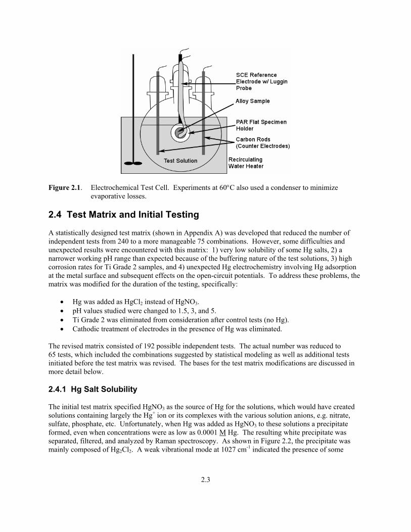
2.3 Electrochemical Test Apparatus Electrochemical testing was performed using a Gamry (Warrington, PA) CMS Electrochemical Measurement System. A standard 3-electrode arrangement (working, counter, and reference electrodes) was used, similar to that described in ASTM G61 (and diagrammed in Figure 2.1).(a) The working electrode was the test specimen mounted in a Perkin Elmer Princeton Applied Research (Oak Ridge, TN) circular flat specimen holder that exposed 1 cm2 of alloy surface to the electrolyte. The counter electrode was a paired set of graphite rods. The reference electrode was an SCE with a Luggin probe bridge that was positioned a few millimeters from the surface of the test specimen. Temperature was controlled by a recirculating water bath in which the test vessel was immersed. Temperature was measured with an Hg thermometer inserted in the test solution. For experiments at 60°C, a reflux column was used to minimize loss of solution to the vapor phase. X-ray photoelectron spectroscopy (XPS) measurements were made with a Phi (Eden Prairie, MN) Quantum 2000 spectrometer. The Raman spectrometer used was a Spex (Edison, NJ) model 1877 triple monochromator spectrometer with a 488.0-nm line of a Coherent (Santa Clara, CA) Ar+ laser for excitation.

(a) As described in Section 2.4.2, conditions of the test solutions favored the formation of HF. While the presence

of HF normally precludes the use of glass containers (HF dissolves silica), analysis of solutions after testing showed that the dissolution rate of the glass was small, which, combined with the likelihood that any dissolved silica would be complexed in the solutions, indicated that the influence of silica on the corrosion rates was minimal as long as the tests were completed in a few hours. All experiments were completed within this time frame.

2.3

Figure 2.1. Electrochemical Test Cell. Experiments at 60°C also used a condenser to minimize

evaporative losses. 2.4 Test Matrix and Initial Testing A statistically designed test matrix (shown in Appendix A) was developed that reduced the number of independent tests from 240 to a more manageable 75 combinations. However, some difficulties and unexpected results were encountered with this matrix: 1) very low solubility of some Hg salts, 2) a narrower working pH range than expected because of the buffering nature of the test solutions, 3) high corrosion rates for Ti Grade 2 samples, and 4) unexpected Hg electrochemistry involving Hg adsorption at the metal surface and subsequent effects on the open-circuit potentials. To address these problems, the matrix was modified for the duration of the testing, specifically:

• Hg was added as HgCl2 instead of HgNO3. • pH values studied were changed to 1.5, 3, and 5. • Ti Grade 2 was eliminated from consideration after control tests (no Hg). • Cathodic treatment of electrodes in the presence of Hg was eliminated.

The revised matrix consisted of 192 possible independent tests. The actual number was reduced to 65 tests, which included the combinations suggested by statistical modeling as well as additional tests initiated before the test matrix was revised. The bases for the test matrix modifications are discussed in more detail below. 2.4.1 Hg Salt Solubility The initial test matrix specified HgNO3 as the source of Hg for the solutions, which would have created solutions containing largely the Hg+ ion or its complexes with the various solution anions, e.g. nitrate, sulfate, phosphate, etc. Unfortunately, when Hg was added as HgNO3 to these solutions a precipitate formed, even when concentrations were as low as 0.0001 M Hg. The resulting white precipitate was separated, filtered, and analyzed by Raman spectroscopy. As shown in Figure 2.2, the precipitate was mainly composed of Hg2Cl2. A weak vibrational mode at 1027 cm-1 indicated the presence of some

2.4

0

1000

2000

3000

4000

5000

6000

7000

200 300 400 500 600 Raman Shift, cm-1

Precipitate

Ram

an In

tens

ity, a

rbitr

ary

units

HgCl2 (calomel)

Figure 2.2. Raman Spectrum of Precipitate Formed When HgNO3 Was Added to Test Solution. Positive

ID for Hg2Cl2 is shown. Hg2SO4 as well. This result is consistent with the low solubility of Hg2Cl2 in cold water, 4.2E-6 M (Weast 1979); however, it was not expected that the salt would be so insoluble in the pH 1.5 stock solution used. To address the solubility problem, Hg2+ salts [e.g., Hg(NO3)2, HgCl2] were considered instead. HgCl2 was found to be most suitable with a reported solubility of 0.25 M in cold water (Weast 1979). HgCl2 was soluble in all of the solutions tested in this work, and consequently became the Hg source for further testing. For solutions with 0.01M Hg, the amount of chloride added as HgCl2 was significant relative to the amount added as HCl or NaCl (see Table 3.1 in Section 3.0). For these solutions, the amount of HCl or NaCl was therefore adjusted so that the total amount of chloride was 0.1 M as required by the test matrix. For solutions with less than 0.01 M Hg (i.e., 0.001 M or lower), the adjustment was considered unnecessary. 2.4.2 pH Range of Solutions Problems were also encountered trying to achieve the target pH values of the solution, specifically pH 0 and pH 1. First, the glass pH electrode was unsuitable for measuring pH of these solutions at pH values below about 3. At this pH, hydrogen fluoride (HF) forms due to equilibria involving H+ and F- ions (pK of HF is 3.45 at 25°C; Weast 1979), and subsequently interferes with the operation of the glass pH electrode. When the electrode is immersed in solutions with pH 3 or lower, the pH measurement drifts higher due to interaction with HF. Consequently, pH test paper strips were used. The estimated uncertainty for these measurements was ± 0.5 pH units. The pH of the solutions could not be made lower than 1.5, because of a buffering action from the combination of weak acids that were part of the mixture, i.e., hydrofluoric acid, citric acid, and the

2.5

hydrogen sulfates and phosphates. The combined effect was a pH range between 1 and 1.5 (nominally 1.5) when almost all the ingredients were added in their acid form. Therefore, the tests planned at pH 0 could not be performed, and those at pH 1 were considered to be pH 1.5. Studies at pH 3 and 5 were not affected. 2.4.3 Ti Grade 2 Corrosion The Ti Grade 2 specimens exhibited extremely high corrosion rates even without Hg. Corrosion rates on the order of 103 mils per year (mpy), for example, were measured in the absence of Hg at 40°C and 60°C at several pH values using both polarization resistance and Tafel methods. As illustrated in Figure 2.3, the cyclic polarization curves for Ti Grade 2 showed a “flat” region that could be characteristic of a passive region. However, the current density at that region was much too high to be passive. The Ti Grade 2 clearly was unsuitable for use in these solutions with or without Hg, and was not tested further.

Figure 2.3. Cyclic Polarization Curve for Ti Grade 2 Sample at pH 1.5, 40°C, and 0 M Hg Concentration. Note that current density in the vertical (constant current) portion of the curve is very high, approximately 1 mA/cm2, indicating non-passive behavior.

2.4.4 Hg Electrochemistry In understanding why the test matrix was modified, it should be noted here that the cyclic polarization curves were initiated from the open circuit potential, instead of from more negative potentials, because Hg2+ ions were observed to interact with the metal surfaces, apparently coating them with a layer of metallic Hg. The alloy surface/solution interaction was a primary focus of this study. Any cathodic treatment, a typical step for the cyclic polarization method, caused Hg to form on the surface and obscure

2.6

the results. While this interaction was also observed even without cathodic treatment, it was anticipated that additional Hg deposition, occurring upon cathodic polarization, would further complicate interpretation of the results.

Figure 2.4 shows cyclic polarization curves for two Hg concentrations that include a small amount of cathodic treatment. Notice that the current density between -0.2 V and 0.1 V upon the initial sweep (beginning at cathodic potentials) has a direct relationship to Hg concentration. Increasing Hg concentration tenfold resulted in an order of magnitude increase in current density in this region. Since all other conditions, including pH, were constant, this result shows that the reduction of Hg plays an important role in the cathodic reaction. Subsequently, sweeping to the anodic side of the open circuit potential resulted in the appearance of some small sudden jumps and features that can be associated with Hg reoxidation. Obviously, in this study that focuses on the corrosion properties of the working electrode material, it is undesirable to have Hg redox chemistry (occurring independently to the corrosion reactions) interfere with the analysis. To minimize this interference, all steps involving cathodic treatment of the electrodes in the presence of Hg were eliminated.

Figure 2.4. Cyclic Polarization Curves for 6% Mo Sample at pH 1.5, 20°C, and Two Hg Concentrations. Anodic branches for both Hg concentrations are identical. Current density of cathodic branches depends on Hg concentration.

3.1

3.0 Results and Discussion The results of the electrochemical testing are discussed here, including the results noted in Section 2.4 that led to the changes in the test matrix and procedures. The results of measurements of the two key quantifiable parameters, corrosion potential and corrosions rates, are presented, as well as the more qualitative results associated with cyclic polarization curves. The cyclic polarization curves were also used to extract another quantifiable parameter, the passive current density. Table 3.1 summarizes the corrosion testing.

Table 3.1. Summary of Experiments and Results

Test No. Alloy

Temp. (°C) pH

Hg Conc. (M)

Corrosion Potential Ecorr (mV)

Corrosion Rate

(mpy)

Passive Current Density (A/cm2)

1 304L SS 20 1.5 0 -178.7 0.302 -5.3 2 20 1.5 0.001 113.8 0.187 -5.0 3 20 1.5 0.0001 122.0 (a) (a) 4 20 3 0.01 117.9 0.120 -5.0 5 20 3 0.0001 115.8 0.088 -5.0 6 20 5 0.001 116.0 0.333 -5.1 7 40 1.5 0.0001 121.3 0.211 -5.0 8 40 1.5 0.01 132.4 0.243 -4.8 9 40 1.5 0.001 126.3 0.212 -4.9

10 40 3 0 -290.9 0.963(b) -5.3 11 40 5 0.0001 120.7 0.205 -5.0 12 60 1.5 0.01 139.8 0.291 -4.9 13 60 1.5 0 -321.0 (b) -5.3 14 60 1.5 0.0001 134.4 (c) (c) 15 60 3 0.001 130.8 0.113 -4.9 16 60 5 0 -311.1 0.041 -5.1

1 316L SS 20 1.5 0.01 124.1 0.373 -4.9 2 20 1.5 0.001 129.8 0.498 -4.9 3 20 1.5 0 -210.9 0.986 -5.2 4 20 3 0 -143.4 0.422 -5.3 5 20 3 0.001 118.3 0.155 -5.0 6 20 5 0.0001 119.5 0.636 -4.9

3.2

Table 3.1. (contd)

Test No. Alloy

Temp. (°C) pH

Hg Conc. (M)

Corrosion Potential Ecorr (mV)

Corrosion Rate

(mpy)

Passive Current Density (A/cm2)

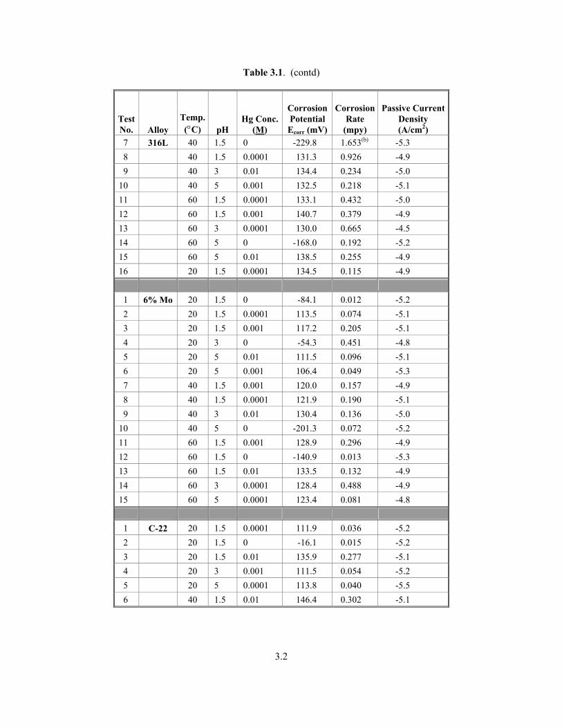
7 316L 40 1.5 0 -229.8 1.653(b) -5.3 8 40 1.5 0.0001 131.3 0.926 -4.9 9 40 3 0.01 134.4 0.234 -5.0

10 40 5 0.001 132.5 0.218 -5.1 11 60 1.5 0.0001 133.1 0.432 -5.0 12 60 1.5 0.001 140.7 0.379 -4.9 13 60 3 0.0001 130.0 0.665 -4.5 14 60 5 0 -168.0 0.192 -5.2 15 60 5 0.01 138.5 0.255 -4.9 16 20 1.5 0.0001 134.5 0.115 -4.9

1 6% Mo 20 1.5 0 -84.1 0.012 -5.2 2 20 1.5 0.0001 113.5 0.074 -5.1 3 20 1.5 0.001 117.2 0.205 -5.1 4 20 3 0 -54.3 0.451 -4.8 5 20 5 0.01 111.5 0.096 -5.1 6 20 5 0.001 106.4 0.049 -5.3 7 40 1.5 0.001 120.0 0.157 -4.9 8 40 1.5 0.0001 121.9 0.190 -5.1 9 40 3 0.01 130.4 0.136 -5.0

10 40 5 0 -201.3 0.072 -5.2 11 60 1.5 0.001 128.9 0.296 -4.9 12 60 1.5 0 -140.9 0.013 -5.3 13 60 1.5 0.01 133.5 0.132 -4.9 14 60 3 0.0001 128.4 0.488 -4.9 15 60 5 0.0001 123.4 0.081 -4.8

1 C-22 20 1.5 0.0001 111.9 0.036 -5.2 2 20 1.5 0 -16.1 0.015 -5.2 3 20 1.5 0.01 135.9 0.277 -5.1 4 20 3 0.001 111.5 0.054 -5.2 5 20 5 0.0001 113.8 0.040 -5.5 6 40 1.5 0.01 146.4 0.302 -5.1

3.3

Table 3.1. (contd)

Test No. Alloy

Temp. (°C) pH

Hg Conc. (M)

Corrosion Potential Ecorr (mV)

Corrosion Rate

(mpy)

Passive Current Density (A/cm2)

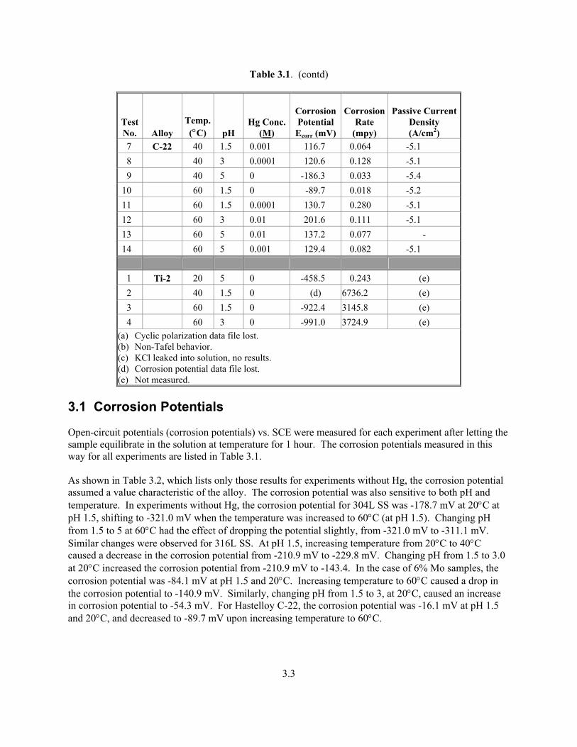
7 C-22 40 1.5 0.001 116.7 0.064 -5.1 8 40 3 0.0001 120.6 0.128 -5.1 9 40 5 0 -186.3 0.033 -5.4

10 60 1.5 0 -89.7 0.018 -5.2 11 60 1.5 0.0001 130.7 0.280 -5.1 12 60 3 0.01 201.6 0.111 -5.1 13 60 5 0.01 137.2 0.077 - 14 60 5 0.001 129.4 0.082 -5.1

1 Ti-2 20 5 0 -458.5 0.243 (e) 2 40 1.5 0 (d) 6736.2 (e) 3 60 1.5 0 -922.4 3145.8 (e) 4 60 3 0 -991.0 3724.9 (e)

(a) Cyclic polarization data file lost. (b) Non-Tafel behavior. (c) KCl leaked into solution, no results. (d) Corrosion potential data file lost. (e) Not measured.

3.1 Corrosion Potentials Open-circuit potentials (corrosion potentials) vs. SCE were measured for each experiment after letting the sample equilibrate in the solution at temperature for 1 hour. The corrosion potentials measured in this way for all experiments are listed in Table 3.1. As shown in Table 3.2, which lists only those results for experiments without Hg, the corrosion potential assumed a value characteristic of the alloy. The corrosion potential was also sensitive to both pH and temperature. In experiments without Hg, the corrosion potential for 304L SS was -178.7 mV at 20°C at pH 1.5, shifting to -321.0 mV when the temperature was increased to 60°C (at pH 1.5). Changing pH from 1.5 to 5 at 60°C had the effect of dropping the potential slightly, from -321.0 mV to -311.1 mV. Similar changes were observed for 316L SS. At pH 1.5, increasing temperature from 20°C to 40°C caused a decrease in the corrosion potential from -210.9 mV to -229.8 mV. Changing pH from 1.5 to 3.0 at 20°C increased the corrosion potential from -210.9 mV to -143.4. In the case of 6% Mo samples, the corrosion potential was -84.1 mV at pH 1.5 and 20°C. Increasing temperature to 60°C caused a drop in the corrosion potential to -140.9 mV. Similarly, changing pH from 1.5 to 3, at 20°C, caused an increase in corrosion potential to -54.3 mV. For Hastelloy C-22, the corrosion potential was -16.1 mV at pH 1.5 and 20°C, and decreased to -89.7 mV upon increasing temperature to 60°C.

3.4

Table 3.2. Results of Experiments Without Hg

Test No. Alloy

Temp. (°C) pH

Corrosion Potential Ecorr

(mV) 1 304L SS 20 1.5 -178.7

10 40 3 -290.9 13 60 1.5 -321.0 16 60 5 -311.1

3 316L SS 20 1.5 -210.9 4 20 3 -143.4 7 40 1.5 -229.8

14 60 5 -168.0

1 6% Mo 20 1.5 -84.1 4 20 3 -54.3

10 40 5 -201.3 12 60 1.5 -140.9

2 C-22 20 1.5 -16.1 9 40 5 -186.3

10 60 1.5 -89.7

1 Ti-2 20 5 -458.5 2 40 1.5 (a) 3 60 1.5 -922.4 4 60 3 -991.0

(a) Corrosion potential data file lost. The above observations strongly indicate that, in the absence of Hg, increasing temperature has the general effect of decreasing the corrosion potential, while increasing pH tends to cause an increase in the corrosion potential. Normally, the corrosion potential is expected to decrease with increasing pH (assuming the only effect is on the cathodic reaction) in accordance with the Nernst Equation for the cathodic reaction: 2H+ + 2e = H2 (E = 0 - 0.059 pH); however, the opposite was observed. Although the specific reasons for these shifts cannot be determined from the limited number of experiments performed in this work, the most likely cause is shifts in the equilibria of the various dissolved species with both temperature and pH and their effect on the surface film. Likely species include HF, hydrogen sulfates, hydrogen phosphates, and citric acid, as well as water. More important for the purposes of this work is the effect of Hg on the corrosion potentials. As shown in Table 3.1, a very unexpected result occurs when Hg is present at any concentration for any of the alloys tested. In the presence of Hg, the corrosion potential assumes an average value of around 130 mV.

3.5

(Actual average is 127 mV.) There is a very slight systematic change in the corrosion potential with order of magnitude increases in Hg. For example, the corrosion potential for 304L SS at 40°C and pH 1.5 increases from 121.3 mV to 126.3 mV to 132.4 mV as Hg is increased from 0.0001 to 0.001 to 0.01 M, respectively. Similarly, there are slight increases in the corrosion potential with Hg concentration for the 6% Mo and C-22 samples. However, slight systematic decreases are also observed as, for example, in the case of 316L SS. Since these are changes for order of magnitude variations in Hg, they can be considered small compared to the difference between the corrosion potentials with no Hg and at the lowest Hg concentration. The effect of Hg on the corrosion potentials of the alloys tested in this work may be explained by the reported tendency of Hg to adsorb (as elemental Hg) in thin or monolayer coverages on metal oxide surfaces (Davis 1996). Should this occur, the Hg would effectively isolate the alloy under study from the solution, and the working electrode would become an Hg electrode in contact with the bulk electrolyte. Since Cl- ions are in abundance, and given that Hg2Cl2 is so poorly soluble and likely the result of the first oxidation step of metallic Hg, it is reasonable that the test alloy working electrodes, after equilibration in the solution, become effectively a calomel-like electrode with the half-cell reaction: Hg2Cl2(s) + 2e = 2Hg(l) + 2Cl-(aq). Since this is precisely the same half reaction occurring at the reference electrode, the potential difference between the working (w) and reference (r) electrodes would be given by -0.0592log[Cl-(w)/Cl-(r)], where the Cl- term refers to chloride activities at the working and reference electrodes, plus any junction potentials that may exist between the working and reference electrodes. For this study, the chloride concentration at the working electrode is the concentration in the simulant solution (0.1 M), and the chloride concentration in the reference electrode is given by the solubility of KCl (approximately 3.19 M). Assuming solution ideality (activity equals concentration) and ignoring any junction potentials, this leads to a calculated potential difference of about +89 mV, which is reasonably close to the observed “corrosion” potentials of about 130 mV. The difference between the calculated +89 mV and the observed 130 mV may be due to a lower concentration of Cl- in solution than expected from the batch formulations. Given the high ionic strength of this media, it would not be surprising if some of the Cl- was associated with other ions in the electrolyte (i.e., solution non-ideality). There may also be significant junction potentials between the working and reference electrodes that may contribute to larger-than-expected potential differences. The junction potentials could arise from differences in ionic strengths between the working and reference electrode solutions as well as differences in temperature. The presence of Hg on the working electrode surface was confirmed by XPS on one of the 304L SS electrodes. This result is consistent with the observation of a thin film, presumably a mixture of Hg metal and calomel, that had deposited on specimen surfaces during testing. This analysis shows that the corrosion kinetics for the alloys under study is difficult to determine electrochemically in the presence of Hg. The Hg (in solution) deposits on the surface of the metal as a thin, probably monolayer, film, raising the potential to that of the calomel electrode, and thus obscuring the corrosion behavior of the alloy underneath. 3.2 Corrosion Rates Because of the problems associated with Hg deposition, it was decided that any method that used cathodic polarization (applying a potential to the corrosion sample that is more negative than the open-circuit potential) would cause more Hg to deposit and complicate the results. Therefore, a Tafel analysis was used for calculating corrosion rates. In a Tafel measurement, the corrosion rate is obtained by first

3.6

determining the corrosion current from the intersection of two of the following three characteristics of the potential vs. log current-density plots: corrosion potential, anodic Tafel slope, and cathodic Tafel slope. In the present study, only the corrosion potential and anodic Tafel slope were used to determine the corrosion current (Icorr), as shown in Figure 3.1. The resulting corrosion current was then used to calculate the corrosion rate according to the following equation:

Corrosion Rate (mpy) = ndA

M10x28.1I5

corr

where: Icorr = corrosion current (A) M = molecular weight (g/mol) n = number of electrons transferred in the corrosion reaction d = density of the metal (g/cm3) A = area of the metal specimen (cm2)

Figure 3.1. Schematic Presentation of Strategy Used to Determine Corrosion Current Density, Icorr.

Since cathodic branch was not obtained, corrosion current was determined from anodic Tafel slope and corrosion potential, Ecorr.

The corrosion rates determined in this way are listed in Table 3.1. Estimated uncertainties, based on adjusting fits to the Tafel curves, were ±10% for all entries except Experiments #10 for 304L SS and #7 for 316L SS, which were ±20% and ±100%, respectively. The latter was sufficiently large to consider this experimental point a “flyer.” A statistical analysis was performed on the corrosion rates, and the results are given in Appendix B. The primary conclusions from the statistical treatment are given below:

• The corrosion rates for the tested alloys for almost all conditions (Hg concentration, pH, and temperature) were approximately 1 mpy or less. (One experiment for 316L SS gave a somewhat higher value.) Of these measurements, most values were on the order of 0.2 mpy or less.

3.7

• The principal parameter influencing the corrosion rate was the alloy composition. Averages of all of the corrosion rates for the same alloys indicated that 316L exhibited the highest corrosion rates, followed by 304L SS, 6% Mo, and Hastelloy C-22, although the latter three were statistically very similar with large overlapping uncertainties.

• Increasing Hg concentration had the apparent effect of decreasing corrosion rate, although this can be attributed largely to the discontinuous shift of open-circuit potential with even the smallest Hg addition.

• Increasing the pH had the effect of slightly decreasing the corrosion rate.

• Temperature had no significant effect on corrosion rate over the range of temperatures studied, 20°C to 60°C.

Although the corrosion rates showed a dependence on alloy composition, the rates were small (except for Ti Grade 2), approximately 1 mpy or less. Based on the short-term tests performed in this work alone, therefore, any of the Fe-Ni-Cr alloys tested appear to be suitable, depending on the conditions. As shown in Figure 3.2, it appears that the trend in the average corrosion rate with alloy composition is determined at least partly by the Cr content of the alloys. Of the alloys tested, 6% and Hastelloy C-22 had the best

0

0.1

0.2

0.3

0.4

0.5

16 17 18 19 20 21 22

%Cr

316L SS

304L SS

6% Mo

C-22

0.6

Cor

rosi

on R

ate,

mpy

Figure 3.2. Variation of Average Corrosion Rate of Alloy Samples in Tests Without Hg as a Function of

Cr Concentration in the Alloy corrosion properties, although the 304L SS may be statistically equivalent. This conclusion is based on short-term measurements, and the implications of an adsorbed Hg layer on longer-term exposure add uncertainty. The apparently small decrease in corrosion rate with increasing Hg concentration should be interpreted with caution. Upon introduction of even the smallest concentration of Hg (0.0001 M), the open-circuit potential shifts to a potential (approximately 130 mV) that appears to be largely determined by the calomel half-cell reaction, as described in Section 3.1. Because of this shift, the corrosion current would

3.8

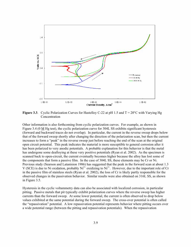
also be expected to shift to a value partly determined by the anodic current at this potential (see Section 3.3). For this reason, the effect of Hg appears the strongest with this first, very small, addition of Hg. As the concentration of Hg is increased above this value, the dependence is much weaker and more uncertain. Hence, the influence of Hg is not so much from its concentration in solution as from the presence of the thin layer of Hg metal that appears to adsorb on the surface of the alloy. This thin layer is apparently present for all Hg concentrations and is responsible for the discontinuous shift of corrosion potential from a value determined by the alloy composition to a potential determined by the calomel half-cell reaction. Moreover, the corrosion current in the presence of Hg was determined from the Tafel fit to the cyclic polarization data near the open-circuit potential. This is essentially an estimate of the corrosion current from polarization data at a potential for the calomel half-reaction. Since the form of the polarization curve at this potential is also partly determined by the calomel half-cell reaction itself, associating the kinetics in the vicinity of this potential to the corrosion reaction alone is problematic. Nevertheless, it provides a reasonable estimate (at least as an upper bound) for the behavior of the alloy in the presence of the adsorbed Hg layer. 3.3 Cyclic Polarization Curves Cyclic polarization curves, such as Figure 3.3, can be used in conjunction with open-circuit potential and corrosion rate measurements to evaluate the susceptibility of metals to corrosion. In a cyclic polarization experiment, potential is scanned anodically (to more positive potentials), and current is measured. Upon reaching some “vertex” potential (generally 1.2 V or 1.5 V vs. SCE, in this work), the direction of the scan is reversed and the potential is scanned back to the original open-circuit potential. These cyclic measurements are especially useful in providing important mechanistic information on passive films if they are present. In particular, evidence for passive layers is provided by potential regions where the current density remains small, on the order of 10-6 to 10-5 A/cm2. The wider these regions are (larger potential range), the more passive-like a metal usually is and the more resistant it is to corrosion, particularly in environments where fluctuations in redox conditions (e.g., dissolved oxygen concentration) tend to occur. 3.3.1 Tests Without Hg All specimens tested in this work exhibited passive regions. For example, as shown in Figure 3.3 (0 M Hg test), Hastelloy C-22 has a region between approximately 0.3 V and 0.9 V, where the current density is essentially constant at 10-5A/cm2. The breakdown potential is regarded as the potential where the current begins to increase rapidly at the end of the passive region. In cases where pitting is observed, this breakdown potential normally can be associated with the pitting potential. For Hastelloy C-22, the breakdown potential occurs at about 0.9 V (SCE).

3.9

Figure 3.3. Cyclic Polarization Curves for Hastelloy C-22 at pH 1.5 and T = 20°C with Varying Hg

Concentration Other information is also forthcoming from cyclic polarization curves. For example, as shown in Figure 3.4 (0 M Hg test), the cyclic polarization curve for 304L SS exhibits significant hysteresis (forward and backward traces do not overlap). In particular, the current in the reverse sweep drops below that of the forward sweep shortly after changing the direction of the polarization scan, but then the current increases to form a “peak” in the reverse sweep just before reaching the end of the scan at the original open circuit potential. This peak indicates the material is more susceptible to general corrosion after it has been polarized to very anodic potentials. A probable explanation for this behavior is that the metal has undergone some dealloying at these very positive potentials (Ryan et al. 2002). As the specimen is scanned back to open-circuit, the current eventually becomes higher because the alloy has lost some of the components that form a passive film. In the case of 304L SS, these elements may be Cr or Ni. Previous study (Searson and Latanision 1986) has suggested that the peak in the forward scan at about 1.3 V (SCE) is due to Ni oxidation, probably Ni2+ oxidizing to Ni3+. However, due to the important role of Cr in the passive film of stainless steels (Ryan et al. 2002), the loss of Cr is likely partly responsible for the observed changes in the passivation behavior. Similar results were also obtained on 316L SS, as shown in Figure 3.5. Hysteresis in the cyclic voltammetry data can also be associated with localized corrosion, in particular pitting. Passive metals that pit typically exhibit polarization curves where the reverse sweep has higher currents than the forward sweep. At some lower potential, the current is often observed to drop below values exhibited at the same potential during the forward sweep. The cross-over potential is often called the “repassivation” potential. A low repassivation potential represents behavior where pitting occurs over a wide potential range (between the pitting and repassivation potentials). When the repassivation

3.10

Figure 3.4. Cyclic Polarization Curves for 304L Stainless Steel at pH 1.5 and T = 20°C with Varying

Hg Concentration

Figure 3.5. Cyclic Polarization Curves for 316L Stainless Steel at pH 1.5 and T = 20°C with Varying

Hg Concentration

3.11

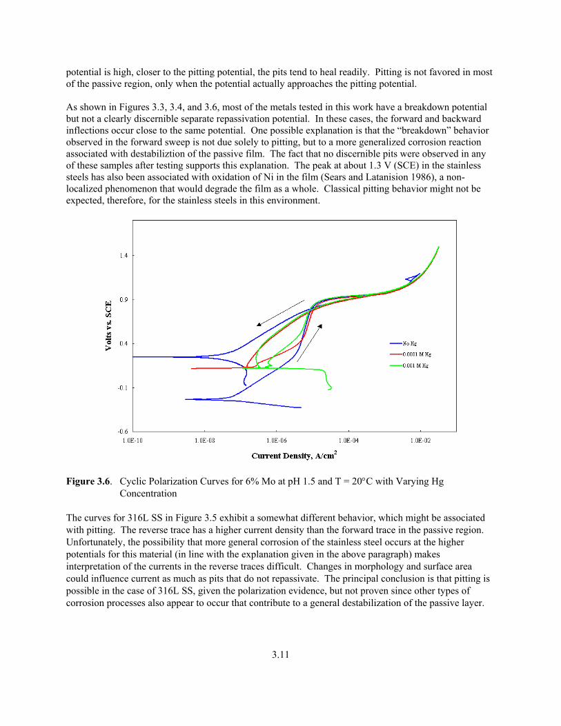
potential is high, closer to the pitting potential, the pits tend to heal readily. Pitting is not favored in most of the passive region, only when the potential actually approaches the pitting potential. As shown in Figures 3.3, 3.4, and 3.6, most of the metals tested in this work have a breakdown potential but not a clearly discernible separate repassivation potential. In these cases, the forward and backward inflections occur close to the same potential. One possible explanation is that the “breakdown” behavior observed in the forward sweep is not due solely to pitting, but to a more generalized corrosion reaction associated with destabiliztion of the passive film. The fact that no discernible pits were observed in any of these samples after testing supports this explanation. The peak at about 1.3 V (SCE) in the stainless steels has also been associated with oxidation of Ni in the film (Sears and Latanision 1986), a non-localized phenomenon that would degrade the film as a whole. Classical pitting behavior might not be expected, therefore, for the stainless steels in this environment.

Figure 3.6. Cyclic Polarization Curves for 6% Mo at pH 1.5 and T = 20°C with Varying Hg

Concentration The curves for 316L SS in Figure 3.5 exhibit a somewhat different behavior, which might be associated with pitting. The reverse trace has a higher current density than the forward trace in the passive region. Unfortunately, the possibility that more general corrosion of the stainless steel occurs at the higher potentials for this material (in line with the explanation given in the above paragraph) makes interpretation of the currents in the reverse traces difficult. Changes in morphology and surface area could influence current as much as pits that do not repassivate. The principal conclusion is that pitting is possible in the case of 316L SS, given the polarization evidence, but not proven since other types of corrosion processes also appear to occur that contribute to a general destabilization of the passive layer.

3.12

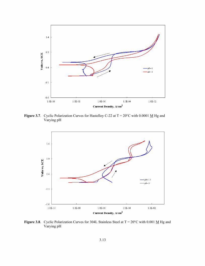
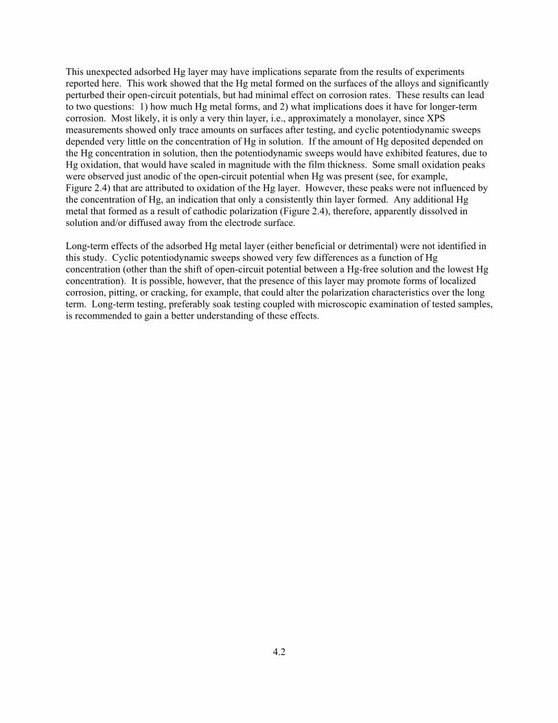
Another type of hysteresis behavior was observed for the Hastelloy C-22 and the 6% Mo alloys. The reverse sweeps for these samples (Figure 3.3 and 3.6) showed a dramatic shift of the corrosion potential to more anodic values. This shift may result from oxygenation of the solution that occurred during high anodic polarization and/or the significant amount of etching that occurred when the samples were polarized to 1.2 V (SCE) and beyond. 3.3.2 Tests With Hg This section addresses how Hg influences the specific characteristics of the curves described above. Since not all combinations of conditions (alloy composition, Hg concentration, temperature, and pH) were tested, it should be recognized that not all the comparisons of the curves are complete. However, some comparisons can be made that suggest the more obvious trends in the effects of the Hg, as well as separate effects of pH and temperature. As indicated in Section 3.2, the primary effect of the Hg is to shift the open-circuit potential from a value determined largely by the alloy composition to approximately 130 mV, a value that appears to be poised by the half-cell reaction of calomel. It can be argued that the calomel half-cell reaction becomes dominant due to the formation of a layer of adsorbed Hg metal in contact with a 0.1 M Cl- solution, and some calomel salt, Hg2Cl2, which, because of its very low solubility, can also precipitate on the surface with only minimal oxidative dissolution of the Hg metal. Above the poised electrode potential, the cyclic polarization curves for most of the Hg-containing solutions with all alloys overlap the control curves obtained in the absence of Hg (see Figures 3.3 through 3.6). Upon reversing the scan direction, after the vertex potential is reached, the curves show varied behavior. However, most of these return sweeps are difficult to explain and depend on the type of corrosion that occurs at the high currents typically exhibited at the vertex potential. Some of the Hastelloy C-22 samples, for example, were observed to etch significantly when swept to this potential. In the case of 304L SS and 316L SS, as another example, there appears to be a peak around 1.4 V in the forward sweep. This peak has been assigned to decomposition of the passive film by oxidation of Ni (Searson and Latanision 1986), but may also involve Cr chemistry. Assuming that the film is changed or, alternatively, that the metal is dealloyed at around 1.4 V, the reverse sweep could exhibit higher currents due to such transformations. As shown in Figures 3.3 and 3.4, the reverse sweeps show a peak at around 0 V that may be due to corrosion of the depassivated or dealloyed metal once it has undergone such transformations at the vertex potential. Notice that Hg has very little influence on both the peak at 1.4 V and the form of the curve during the reverse sweep. It is also important to notice that the forward and reverse sweeps at higher applied potentials show very little, if any, hysteresis. Even though a “breakdown” potential might be determined, there is very little evidence that this breakdown is localized. All tested samples showed either very little corrosion or, as in the case of the Hastelloy C-22, only uniform attack after sweeping to the vertex potential and back. Consequently, neither a “pitting potential” nor a “repassivation potential” could be adequately determined. Both pH and temperature appear to influence the polarization curves, as shown in Figures 3.7 through 3.10. For pH, the breakdown potential was typically observed to shift to slightly less positive potentials with higher pH, as shown for Hastelloy C-22 and 304L SS in Figure 3.7 and 3.8, respectively. With the stainless steels, the peak at 1.4 V is also observed to change somewhat with pH (Figure 3.8). Again, Hg does not have a major effect on the behavior of these features. Temperature has even less of a noticeable

3.13

Figure 3.7. Cyclic Polarization Curves for Hastelloy C-22 at T = 20°C with 0.0001 M Hg and

Varying pH

Figure 3.8. Cyclic Polarization Curves for 304L Stainless Steel at T = 20°C with 0.001 M Hg and

Varying pH

3.14

effect on the cyclic polarization data, as illustrated in Figures 3.9 and 3.10. The forward sweeps are almost identical at different temperatures. The reverse sweeps show a slight temperature dependence. In particular, the stainless steels show a “deeper” dip in the current density upon sweeping backwards, as illustrated by the 304L sample data in Figure 3.10. The passive current plateau was scrutinized and compared for all the experiments to provide quantitative information from the cyclic polarization curves (in lieu of localized corrosion parameters like pitting potential that were considered inappropriate for these data). The passive current density in this study is defined as the “typical” current density across the low-current-density “plateau” in the forward potential sweep. Although not truly a numerical average because it is estimated as the “typical value” between where the current ends its descent from the active region and where it begins to increase at high potentials (illustrated in Figure 3.11), the parameter is a qualitative indication of the passivity of the alloy. Any influence of Hg on this parameter was considered to be evidence that the Hg, either the adsorbed layer or solution species, may be interacting with the film to some extent and hence altering the passivation reactions that protect these alloys in the test environments. Similar to the corrosion rates, the passive current densities were analyzed statistically for all the measurements taken (Appendix B).

Figure 3.9. Cyclic Polarization Curves for Hastelloy C-22 at pH 1.5 with 0.01 M Hg and Varying

Temperature Not surprisingly, the passive current densities showed trends that were largely consistent with the corrosion rates: • Very low passive current densities for all experiments.

3.15

Figure 3.10. Cyclic Polarization Curves for 304L Stainless Steel at pH 1.5 with 0.001 M Hg and Varying Temperature

Increase Corrosion Increase Corrosion

Figure 3.11. Anodic Polarization Curves With and Without Hg. The anodic shift of corrosion potential

due to Hg results in a smaller passive region and, due to the slight upward slope of the curve in this region, causes the average corrosion current to increase.

3.16

• A dependency on the alloy composition. The 316L SS had the highest passive current density, and C-22 the lowest, but, similar to the corrosion rates, the differences are small and may be considered insignificant.

• Effects of both temperature and pH insignificant. The influence of Hg concentration on the passive current density appeared to be small, similar to the corrosion rate, but opposite in direction. Increasing Hg had the apparent effect of slightly increasing the passive currently density. However, this is believed to be an artifact of the way the parameter was determined. As shown in Figure 3.11, the passive current density was taken as the average of the passive currents across the potential range of the passive region. Because of the discontinuous shift of the corrosion potential upon adding even the smallest amount of Hg (0.0001 M), the potential range of this region was much smaller (and at the higher end of the passive potential region) for Hg-containing solutions than for the control solutions containing no Hg. In turn, the average passive current densities were always smaller for the control experiments. Again, this is a result of the discontinuous shift of the corrosion potential due to the presence of the adsorbed Hg layer and may not reflect a real effect of dissolved Hg on the corrosion properties of the passive film.

4.1

4.0 Conclusions and Recommendations The purpose of the work discussed here was to test candidate materials of construction for WTP process equipment and piping to determine the corrosion behavior of various alloys when exposed to Hg-containing waste solutions/process solutions in the plant. The electrochemical corrosion tests conducted for this work were screening tests for follow-on long-term immersion (soak) testing, and were designed to 1) eliminate unsuitable alloys from further consideration, and 2) identify appropriate test parameters and their ranges for long-term soak testing. These screening tests showed that, because of their very low solubility, mercurous (Hg+) salts were unsuitable for the waste/process solution simulants. (Mercurous nitrate, HgNO3, was the salt originally planned for the test solutions, but further tests showed that the Hg needed to be added as a mercuric, Hg+2, salt. Mercuric chloride, HgCl2, was found to be suitable and was used for the remainder of the corrosion testing.) Of the five alloys tested, 304L SS, 316L SS, 6% Mo (254 SMO), Hastelloy C-22, and Ti Grade 2, the Ti Grade 2 showed a large and significant variance, corroding several orders of magnitude faster than the others, and, consequently, was removed from the test matrix early after testing in the Hg-free solution. If Ti Grade 2 is planned to be used, further evaluation at expected conditions is recommended whether or not Hg is present in the waste stream. The other (Fe-Ni-Cr) alloys exhibited much lower potential for corrosion, yet showed differences in corrosion behavior whether or not Hg was present. In most cases, these differences, while small, are statistically significant. Hastelloy C-22 and 6% Mo had the lowest corrosion rates, followed closely by 304L SS. The 316L SS exhibited slightly higher corrosion rates. The corrosion behavior of the alloys during polarization to very anodic potentials was also different. Interestingly, the Hastelloy C-22 showed a tendency to etch after polarizing to 1.5 V vs. SCE, while the stainless steels appeared to corrode very little at these high potentials. Neither pH values nor potentials were observed to have a large effect on corrosion rates, with or without Hg, over the range of values tested in this work. Increasing the pH appeared to decrease the corrosion rate very slightly, while temperature had no statistically significant effect. Interpretation of the test results was greatly complicated by the formation of a layer of adsorbed Hg metal on the surface of all the alloys studied (disregarding Ti Grade 2). This layer caused the open-circuit potentials of the alloys to rise from a potential characteristic of each alloy composition to a value that was essentially independent of the alloy composition and Hg concentration, i.e., approximately 130 mV vs. SCE. Since all of the alloys exhibited passive behavior at their normal open-circuit potential in the absence of Hg as well as at 130 mV (when Hg was present), the effect of the Hg on the corrosion rate in these experiments was minimal. In fact, the corrosion rate appeared to decrease slightly with the presence of Hg in some cases. However, the corrosion rates were small with or without Hg, less than 1 mpy and on the order of 0.2 mpy in most cases, suggesting that differences measured as a function of Hg concentration may be within the experimental uncertainties.

4.2

This unexpected adsorbed Hg layer may have implications separate from the results of experiments reported here. This work showed that the Hg metal formed on the surfaces of the alloys and significantly perturbed their open-circuit potentials, but had minimal effect on corrosion rates. These results can lead to two questions: 1) how much Hg metal forms, and 2) what implications does it have for longer-term corrosion. Most likely, it is only a very thin layer, i.e., approximately a monolayer, since XPS measurements showed only trace amounts on surfaces after testing, and cyclic potentiodynamic sweeps depended very little on the concentration of Hg in solution. If the amount of Hg deposited depended on the Hg concentration in solution, then the potentiodynamic sweeps would have exhibited features, due to Hg oxidation, that would have scaled in magnitude with the film thickness. Some small oxidation peaks were observed just anodic of the open-circuit potential when Hg was present (see, for example, Figure 2.4) that are attributed to oxidation of the Hg layer. However, these peaks were not influenced by the concentration of Hg, an indication that only a consistently thin layer formed. Any additional Hg metal that formed as a result of cathodic polarization (Figure 2.4), therefore, apparently dissolved in solution and/or diffused away from the electrode surface. Long-term effects of the adsorbed Hg metal layer (either beneficial or detrimental) were not identified in this study. Cyclic potentiodynamic sweeps showed very few differences as a function of Hg concentration (other than the shift of open-circuit potential between a Hg-free solution and the lowest Hg concentration). It is possible, however, that the presence of this layer may promote forms of localized corrosion, pitting, or cracking, for example, that could alter the polarization characteristics over the long term. Long-term testing, preferably soak testing coupled with microscopic examination of tested samples, is recommended to gain a better understanding of these effects.

5.1

5.0 References Davis, J. R., ed. 1996. ASM Specialty Handbook: Carbon and Alloy Steels, p. 409. ASM International, Materials Park, OH. Searson, P. C., and R. M. Latanision. 1986. Corrosion J. 42:161. Weast, R. C., ed. 1979. Handbook of Chemistry and Physics. CRC, 60th edn., Boca Raton, FL.

Appendix A

Original Test Matrix

A.1

Table A.1. Original Test Matrix

Alloy Temp. (°C) pH Hg Conc. (M) Alloy Temp. (°C) pH Hg Conc. (M)

304L SS 20 0 0 6% Mo 40 1 0.0001

304L SS 20 0 0.001 6% Mo 40 3 0.01

304L SS 20 1 0.0001 6% Mo 40 5 0

304L SS 20 3 0.01 6% Mo 60 0 0.001

304L SS 20 3 0.0001 6% Mo 60 1 0

304L SS 20 5 0.001 6% Mo 60 1 0.01

304L SS 40 0 0.0001 6% Mo 60 3 0.0001

304L SS 40 1 0.01 6% Mo 60 5 0.0001

304L SS 40 1 0.001

304L SS 40 3 0 C-22 20 0 0.0001

304L SS 40 5 0.0001 C-22 20 1 0

304L SS 60 0 0.01 C-22 20 1 0.01

304L SS 60 1 0 C-22 20 3 0.001

304L SS 60 1 0.0001 C-22 20 5 0.0001

304L SS 60 3 0.001 C-22 40 0 0.01

304L SS 60 5 0 C-22 40 1 0.001

C-22 40 3 0.0001

316L SS 20 0 0.01 C-22 40 5 0

316L SS 20 0 0.001 C-22 60 0 0

316L SS 20 1 0 C-22 60 1 0.0001

316L SS 20 3 0 C-22 60 3 0.01

316L SS 20 3 0.001 C-22 60 5 0.01

316L SS 20 5 0.0001 C-22 60 5 0.001

316L SS 40 0 0

316L SS 40 1 0.0001 Ti-2 20 0 0.01

316L SS 40 3 0.01 Ti-2 20 1 0.001

316L SS 40 5 0.001 Ti-2 20 1 0.0001

316L SS 60 0 0.0001 Ti-2 20 3 0.01

316L SS 60 1 0.001 Ti-2 20 5 0

316L SS 60 3 0.0001 Ti-2 40 0 0.001

316L SS 60 5 0 Ti-2 40 1 0

316L SS 60 5 0.01 Ti-2 40 3 0.0001

Ti-2 40 5 0.01

6% Mo 20 0 0 Ti-2 40 5 0.0001

6% Mo 20 0 0.0001 Ti-2 60 0 0

6% Mo 20 1 0.001 Ti-2 60 0 0.0001

6% Mo 20 3 0 Ti-2 60 1 0.01

6% Mo 20 5 0.01 Ti-2 60 3 0

6% Mo 20 5 0.001 Ti-2 60 5 0.001

6% Mo 40 0 0.001

Appendix B

Results of Statistical Treatment of Data

B.1

Appendix B

Results of Statistical Treatment of Data The following pages present the analysis of a statistically designed coupon corrosion study. Two responses of interest are discussed: Corrosion Rate and Passivation Current. Factors of interest whose impact on corrosion will be examined are the alloy type, temperature, pH, and Hg levels. Four alloy types are included: 304L SS, 316L SS, 6% Mo, and C-22. Temperatures of 20, 40, and 60°C were used. Although four pH levels were planned, measurement difficulty led to only three levels being recorded: 1.5, 3, and 5. Four Hg levels are 0, 0.0001, 0.001, and 0.01 M. To facilitate the modeling, log to the base 10 was used for the Hg levels with the zero level replaced by -6. The four levels considered for Log Hg are therefore -6, -4, -3, and -2. Potentially 192 different combinations of the intended factor levels could have been run. A “d-optimal” subset of 65 combinations was selected; “d-optimal” experimental designs minimize the uncertainties associated with estimated parameters in the resulting statistical model. Several of the 65 coupons resulted in failed measurements, with 58 usable results subsequently obtained for each corrosion rate and passivation current. With the reduced number of pH levels, these proved adequate for evaluating the main effect and second order interaction models. Corrosion rate results will be discussed first followed by those for passivation current. The figure below and related summary information are discussed on the following page.

Corrosion Rate By Alloy

0

0.2

0.4

0.6

0.8

1

1.2

1.4

1.6

304L SS 316L SS 6% Mo C-22

Alloy

Cor

rosi

on R

ate,

mpy

B.2

Analysis of Variance Source DF Sum of Squares Mean Square F Ratio Prob > F Alloy 3 1.4496753 0.483225 7.5188 0.0003 Error 54 3.4705176 0.064269 C. Total 57 4.9201929 Means for Oneway Anova Level Number Mean Std Error Lower 95% Upper 95% 304L SS 13 0.254538 0.07031 0.1136 0.39551 316L SS 16 0.508688 0.06338 0.3816 0.63575 6% Mo 15 0.163467 0.06546 0.0322 0.29470 C-22 14 0.108357 0.06775 -0.0275 0.24420

The previous figure shows the average corrosion rates for the four alloys. Each plotted point represents one of the 58 experimental trials. The vertical extents of the diamonds indicate uncertainty regions for the estimated means for each alloy. Since some of the diamonds would not intersect vertically when moved laterally, the differences between alloys are deemed statistically significant relative to the variability observed within the alloys. In the summary information below the figure, this significance is indicated by the small “P-value” given to the right as “Prob>F” and equal to 0.0003 (this is the value also listed in the figure title). Statistical P-values can range from 0 to 1, with smaller values indicating the statistical significance of the related feature of interest. Several such P-values will be observed throughout these analyses. This small value of 0.0003 indicates that the observed difference is likely a “real phenomenon” and not simply due to random measurement or experimental variability. In other words, a repeated study would be expected to show similar results. The conclusion derived from the figure above is that the alloys indeed exhibit differing corrosion rates. The vertical variation of the points within each alloy show, however, that knowing the alloy alone is not sufficient to accurately predict the corrosion rate. The alloy differences are significant relative to this variability, but hopefully the other factors, pH, temperature, and Log Hg, will help to explain the additional variability. The model summary information below is a first step in investigating all four factors. Further discussion is on the next page. Corrosion Rate Model (no interaction) Summary of Fit RSquare 0.377361 RSquare Adj 0.30411 Root Mean Square Error 0.245089 Analysis of Variance Source DF Sum of Squares Mean Square F Ratio Model 6 1.8566905 0.309448 5.1516 Error 51 3.0635024 0.060069 Prob > F C. Total 57 4.9201929 0.0003

B.3

Effect Tests Source Nparm DF Sum of Squares F Ratio Prob > F Alloy 3 3 1.3982032 7.7589 0.0002 Temp 1 1 0.0076065 0.1266 0.7234 pH 1 1 0.1996473 3.3237 0.0742 Log Hg 1 1 0.2166127 3.6061 0.0632

Prediction Profiler

Cor

rosi

on R

ate 1.653

-0.017

0.259118

Alloy

304L

SS

316L

SS

6% M

o

C-2

2

Temp

20 6038.2759

pH

1.5 5

2.76724

Log Hg

-6 -2-3.7759

Cor

rosi

on R

ate 1.653

-0.017

0.259118

Alloy

304L

SS

316L

SS

6% M

o

C-2

2

Temp

20 6038.2759

pH

1.5 5

2.76724

Log Hg

-6 -2-3.7759

Note the four P-values in the “Prob>F” column. The very small value 0.0002 for the alloy shows that it is the most important factor in determining the corrosion rate. Next important are each of Log Hg and pH, which impact corrosion of similar magnitude based on their respective P-values, 0.0632 and 0.0742. While the 0.05 level is sometimes considered the “borderline” P-value for declaring a factor a significant influence, the values only slightly larger than 0.05 certainly suggest a reasonable influence on the corrosion rate. On the other hand, the temperature with the large P-value, 0.7234, shows it has virtually no impact on corrosion. The final Profiler illustration figure shows these relationships between corrosion rate and the factors. Other quantities of interest in the previous summary results are the adjusted R-square value listed as “RSquare Adj,” the Root Mean Square Error (RMSE), and the overall Prob>F P-value. While the R-Square value represents the percentage of the variability in corrosion rate explained by the factors, adjusted R-square reduces this value based on the number of parameters included in the model. By increasing the number of model parameters, R-square can always be increased, but more important is the impact on adjusted R-square as we add terms to the model. The larger the adjusted R-square value, the better the model. Similarly, the smaller the overall P-value (0.0003 for this model), the better the model. The RMSE value (here 0.245089) can be thought of as a standard deviation representing the variability not explained by the model. The smaller this value, the better the model. A rather crude interpretation of this value is that given a set of specific factor levels, a predicted corrosion rate could be obtained from the model. The uncertainty associated with this prediction could be thought of as being roughly plus/minus twice the RMSE, or in this case about + 0.49. As terms are added to the model, the impact on adjusted R-square, RMSE, and the overall P-value will be considered. The following summary results are for the model that also includes all the two-way interactions. Two factors have a significant interaction if the impact of one factor changes depending on the level taken on by the other factor. Discussion of this model with interaction terms follows on the next page.

B.4

Corrosion Rate Model (with interaction) Summary of Fit RSquare 0.558322 RSquare Adj 0.35447 Root Mean Square Error 0.236054 Analysis of Variance Source DF Sum of Squares Mean Square F Ratio Model 18 2.7470499 0.152614 2.7389 Error 39 2.1731430 0.055722 Prob > F C. Total 57 4.9201929 0.0042 Effect Tests Source Nparm DF Sum of Squares F Ratio Prob > F Alloy 3 3 1.3998516 8.3741 0.0002 Temp 1 1 0.0178563 0.3205 0.5746 Alloy*Temp 3 3 0.0066549 0.0398 0.9892 pH 1 1 0.1441588 2.5871 0.1158 Alloy* pH 3 3 0.1281478 0.7666 0.5197 Temp* pH 1 1 0.1016754 1.8247 0.1845 Log Hg 1 1 0.2299422 4.1266 0.0491 Alloy*Log Hg 3 3 0.5557099 3.3243 0.0294 Temp*Log Hg 1 1 0.0163463 0.2934 0.5912 pH *Log Hg 1 1 0.0346329 0.6215 0.4352

Prediction Profiler

Cor

rosi

on R

ate 1.653

-0.081

0.272937

Alloy304L

SS

316L

SS

6% M

o

C-2

2

Temp

20 6038.2759

pH

1.5 5

2.76724

Log Hg

-6 -2-3.7759

Cor

rosi

on R

ate 1.653

-0.081

0.272937

Alloy304L

SS

316L

SS

6% M

o

C-2

2

Temp

20 6038.2759

pH

1.5 5

2.76724

Log Hg

-6 -2-3.7759

Some improvement was obtained in this model that contains all the main factors and their interactions. Note the larger adjusted R-square compared to the previous model, and the smaller RMSE. However, the overall P-value actually increased to 0.0042, meaning that this model is slightly less statistically significant. This is because terms that are not really useful have been included. Based on the individual P-values, alloy remains the most important factor (P-value 0.0002) followed by its interaction with Log Hg (P-value 0.0294—the importance of this interaction term will be illustrated later). Next in significant impact is the Log Hg factor (P-value 0.0491), with pH having only marginal impact (P-value 0.1158). Other terms provide little contribution. In particular, temperature and all its interaction terms with the other factors are not useful. The next model removes temperature from the model completely.

B.5

Corrosion Rate Model (omitting terms involving temperature) Summary of Fit RSquare 0.529589 RSquare Adj 0.404145 Root Mean Square Error 0.22679 Analysis of Variance Source DF Sum of Squares Mean Square F Ratio Model 12 2.6056776 0.217140 4.2217 Error 45 2.3145153 0.051434 Prob > F C. Total 57 4.9201929 0.0002 Effect Tests Source Nparm DF Sum of Squares F Ratio Prob > F Alloy 3 3 1.3353080 8.6539 0.0001 pH 1 1 0.1712515 3.3296 0.0747 Alloy*pH 3 3 0.1273378 0.8253 0.4869 Log Hg 1 1 0.1891584 3.6777 0.0615 Alloy*Log Hg 3 3 0.5400798 3.5002 0.0229 pH*Log Hg 1 1 0.0583670 1.1348 0.2924

Prediction Profiler

Cor

rosi

on R

ate

1.653

-0.042

0.268055

Alloy

304L

SS

316L

SS

6% M

o

C-2

2

pH

1.5 5

2.76724

Log Hg

-6 -2-3.7759

Cor

rosi

on R

ate

1.653

-0.042

0.268055

Alloy

304L

SS

316L

SS

6% M

o

C-2

2

pH

1.5 5

2.76724

Log Hg

-6 -2-3.7759

As a result of removing the terms involving temperature, note the increased adjusted R-square, decreased RMSE, and smaller overall P-value for this improved model. The next step is to remove the alloy by the pH interaction term that contributes little to the model. Its removal offers further model improvement. After doing so, then removing the pH by Log Hg interaction term hurts the model slightly, so the optimum model is given as follows.

B.6

Optimum Corrosion Rate Model Summary of Fit RSquare 0.503708 RSquare Adj 0.410653 Root Mean Square Error 0.225548 Analysis of Variance Source DF Sum of Squares Mean Square F Ratio Model 9 2.4783398 0.275371 5.4130 Error 48 2.4418531 0.050872 Prob > F C. Total 57 4.9201929 <.0001 Effect Tests Source Nparm DF Sum of Squares F Ratio Prob > F Alloy 3 3 1.3390106 8.7737 <.0001 pH 1 1 0.1866207 3.6684 0.0614 Log Hg 1 1 0.2092695 4.1137 0.0481 Alloy*Log Hg 3 3 0.5787408 3.7921 0.0161 pH*Log Hg 1 1 0.0598852 1.1772 0.2834

This is the best model for these data and these factors for explaining the observed variability in corrosion rate. The RMSE and overall P-value are the smallest in this sequence of models, and adjusted R-square is the maximum. However, note that the R-square value (not adjusted) of 0.50 shows this model can still explain just one-half of the variability in the corrosion rates. One-half the variability remains unexplained. Some of that variability is simply experimental error, which cannot be directly estimated here, since no factor combinations were replicated. In the experimental design process, the decision was made to include more combinations of factor levels rather than replicating selected combinations. This is a reasonable approach when the focus is to determine the relative impact of the various factors. Note, it has been suggested that using the alloy compositions, in particular for chromium and iron, rather than just the alloy names would result in better ability to explain the corrosion rate. Also note again in the above model summary information the relative importance of the various factors by considering the individual P-values at the bottom right. The remaining corrosion rate discussion graphically illustrates the characteristics of the above model. Recall that the initial figure (discussed on Page B.1) showed the influence of the alloy type. The top four figures on the following page show the relationship of corrosion rate and Log Hg for each of the four alloys. The bottom four figures do the same for pH. In each case, a least-squares regression line is plotted on the figures. The number in parentheses after each alloy name in the titles is the P-value associated with the significance of the slope of the line. Small P-values will be associated with steep slopes (in a positive or negative direction) relative to the observed vertical variability in the data points. Small P-values then again mean the factor has significant impact on the corrosion rate for that alloy. Larger P-values indicate flat lines with minimal slopes and little relationship. Note that the regression line equations are given as well. Looking at the group of four figures for a factor simultaneously reflects the influences quantified in the above model summaries. In particular, the slopes for Log Hg depend fairly strongly on the particular alloy considered. This is why the alloy by Log Hg interaction term is quite significant. The four lines for

B.7

Log Hg are plotted in the same figure on the top of Page B.9. Their intersections and differing slopes again show the significance of their associated interaction term. The lack of such intersecting lines for the pH plots, as shown in their combined figure on the bottom of Page B.9, indicate why the alloy by pH interaction was not significant and therefore dropped from the models above. Note the generally smaller regression line P-values for Log Hg as compared to those for pH. Thus, the greater significance of the Log Hg factor results. The large P-values associated with temperature on Page B.10 show why temperature basically had no effect on corrosion rates.

Corrosion Rate by Log Hg for Each Alloy 304L SS 316L SS Corrosion Rate = 0.0508 - 0.0552 Log Hg Corrosion Rate = -0.0466 - 0.1433 Log Hg

0 0.2 0.4 0.6 0.8

1 1.2 1.4 1.6

Cor

rosi

on R

ate,

mpy

-7 -6 -5 -4 -3 -2 -1Log Hg, M

0

0.2

0.4

0.6

0.8

1

1.2

1.4

1.6

Cor

rosi

on R

ate,

mpy

-7 -6 -5 -4 -3 -2 -1Log Hg, M

6% Mo C-22 Corrosion Rate = 0.1649 + 0.0004 Log Hg Corrosion Rate = 0.2406 + 0.0363 Log Hg

0 0.2 0.4 0.6 0.8

1 1.2 1.4 1.6

Cor

rosi

on R

ate,

mpy

-7 -6 -5 -4 -3 -2 -1

Log Hg, M

0

0.2

0.4

0.6

0.8

1

1.2

1.4

1.6

Cor

rosi

on R

ate,

mpy

-7 -6 -5 -4 -3 -2 -1Log Hg, M

B.8

Corrosion Rate by pH for Each Alloy

304L SS 316L SS Corrosion Rate = 0.2822 - 0.0100 pH Corrosion Rate = 0.7925 - 0.1032 pH

0 0.2 0.4 0.6 0.8

1 1.2 1.4 1.6

Cor

rosi

on R

ate,

mpy

1 2 3 4 5 6pH

0

0.2

0.4

0.6

0.8

1

1.2

1.4

1.6

Cor

rosi

on R

ate,

mpy

1 1.5 2 2.5 3 3.5 4 4.5 5 5.5pH

6% Mo C-22 Corrosion Rate = 0.1941 - 0.0112 pH Corrosion Rate = 0.1762 - 0.0241 pH

0 0.2 0.4 0.6 0.8

1 1.2 1.4 1.6

Cor

rosi

on R

ate,

mpy

1 1.5 2 2.5 3 3.5 4 4.5 5 5.5pH

0

0.2

0.4

0.6

0.8

1

1.2

1.4

1.6

Cor

rosi

on R

ate,

mpy

1 1.5 2 2.5 3 3.5 4 4.5 5 5.5pH

B.9

All Alloys Corrosion Rate by Log Hg Concentration

0 0.2 0.4 0.6 0.8

1 1.2 1.4 1.6

Cor

rosi

on R

ate,

mpy

-7 -6 -5 -4 -3 -2 -1 Log Hg, M

304L SS 316L SS 6% MO C-22

All Alloys Corrosion Rate by pH

0 0.2 0.4 0.6 0.8

1 1.2 1.4 1.6

Cor

rosi

on R

ate,

mpy

1 2 3 4 5pH

304L SS 316L SS 6% MO C-22

B.10

Corrosion Rate by Temperature for Each Alloy 304L SS 316L SS

0 0.2 0.4 0.6 0.8

1 1.2 1.4 1.6

Cor

rosi

on R

ate,

mpy

10 20 30 40 50 60 70Temp, °C

0

0.2

0.4

0.6

0.8

1

1.2

1.4

1.6

Cor

rosi

on R

ate,

mpy

10 20 30 40 50 60 70Temp, °C

6% Mo C-22

0 0.2 0.4 0.6 0.8

1 1.2 1.4 1.6

Cor

rosi

on R

ate,

mpy

10 20 30 40 50 60 70Temp, °C

0

0.2

0.4

0.6

0.8

1

1.2

1.4

1.6

Cor

rosi

on R

ate,

mpy

10 20 30 40 50 60 70

Temp, °C

Attention now turns to modeling Passivation Current. A similar discussion follows, but fewer details are given since the summary results and illustrations use the same concepts as those discussed for the corrosion rate. The figure on the following page shows slightly less impact on passivation current due to alloy type than was observed for corrosion rate. Nonetheless, the differences are statistically significant, as indicated by the P-value of 0.0256. Note the pattern in the alloy means is generally the same for corrosion rate (Page B.1) and passivation current (next page). The alloy 316L SS has the largest mean values, while C-22 has the smallest.

B.11

Passivation Current By Alloy

Log

Pas

siva

tion

Cur

rent

, A

-5.6

-5.4

-5.2

-5

-4.8

-4.6

-4.4

304L SS 316L SS 6% Mo C-22

Alloy

Analysis of Variance Source DF Sum of Squares Mean Square F Ratio Prob > F Alloy 3 0.2822093 0.094070 3.3495 0.0256 Error 54 1.5165838 0.028085 C. Total 57 1.7987931 Means for Oneway Anova Level Number Mean Std Error Lower 95% Upper 95% 304L SS 14 -5.0429 0.04479 -5.133 -4.953 316L SS 16 -4.9938 0.04190 -5.078 -4.910 6% Mo 15 -5.0400 0.04327 -5.127 -4.953 C-22 13 -5.1846 0.04648 -5.278 -5.091

The P-values in the main effect model (no interactions) that follows show the Log Hg is the most influential factor on passivation current, then alloy, and then temperature, all of which have quite significant influence. The factor pH has marginal influence. These relationships are shown in the Profiler figures on the next page. Passivation Current Model (no interaction) Summary of Fit RSquare 0.477563 RSquare Adj 0.416099 Root Mean Square Error 0.135745 Analysis of Variance Source DF Sum of Squares Mean Square F Ratio Model 6 0.8590363 0.143173 7.7699 Error 51 0.9397568 0.018427 Prob > F C. Total 57 1.7987931 <.0001 Effect Tests Source Nparm DF Sum of Squares F Ratio Prob > F Alloy 3 3 0.31142659 5.6336 0.0021 Temp 1 1 0.10968063 5.9523 0.0182 pH 1 1 0.03274171 1.7769 0.1885 Log Hg 1 1 0.43405991 23.5562 <.0001

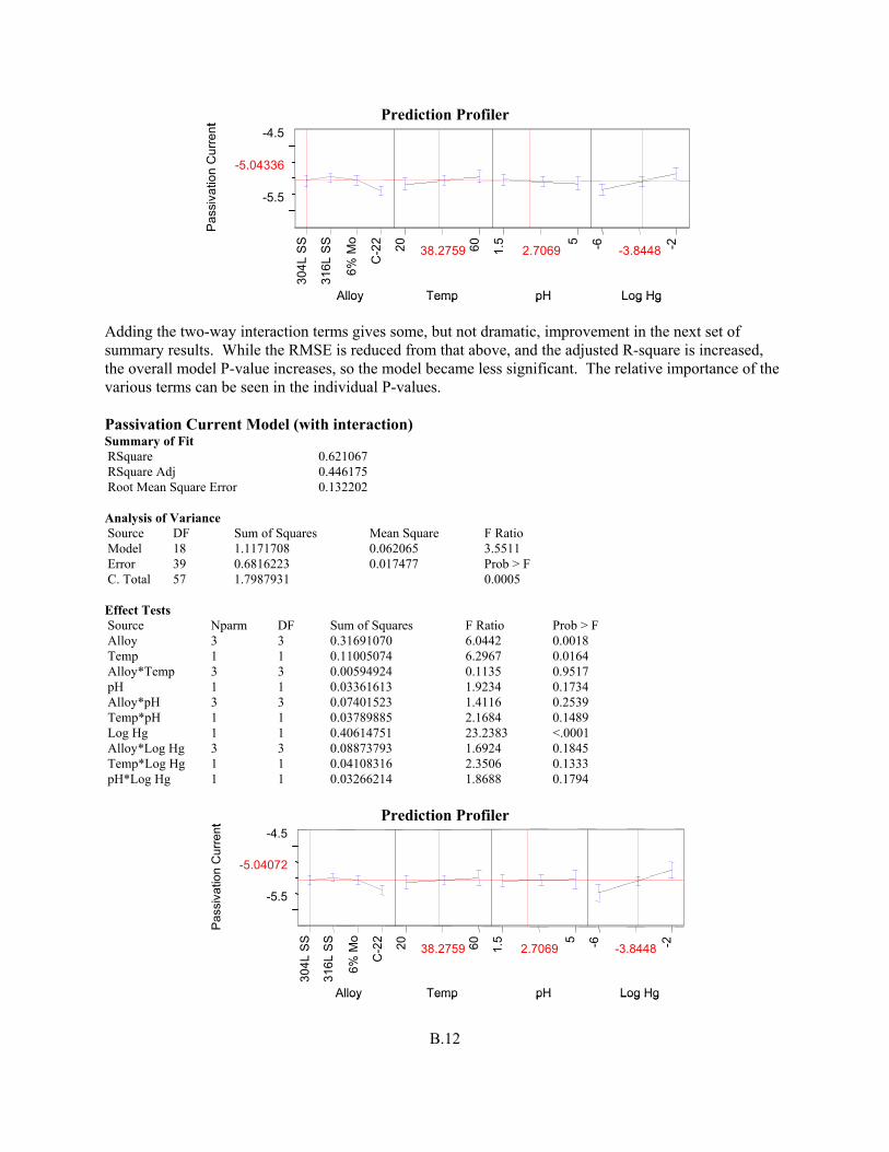
B.12

Prediction Profiler

Pas

siva

tion

Cur

rent -4.5

-5.5

-5.04336

Alloy30

4L S

S

316L

SS

6% M

o

C-2

2

Temp

20 6038.2759

pH

1.5 5

2.7069

Log Hg

-6 -2-3.8448

Pas

siva

tion

Cur

rent -4.5

-5.5

-5.04336

Alloy30

4L S

S

316L

SS

6% M

o

C-2

2

Temp

20 6038.2759

pH

1.5 5

2.7069

Log Hg

-6 -2-3.8448

Adding the two-way interaction terms gives some, but not dramatic, improvement in the next set of summary results. While the RMSE is reduced from that above, and the adjusted R-square is increased, the overall model P-value increases, so the model became less significant. The relative importance of the various terms can be seen in the individual P-values. Passivation Current Model (with interaction) Summary of Fit RSquare 0.621067 RSquare Adj 0.446175 Root Mean Square Error 0.132202 Analysis of Variance Source DF Sum of Squares Mean Square F Ratio Model 18 1.1171708 0.062065 3.5511 Error 39 0.6816223 0.017477 Prob > F C. Total 57 1.7987931 0.0005 Effect Tests Source Nparm DF Sum of Squares F Ratio Prob > F Alloy 3 3 0.31691070 6.0442 0.0018 Temp 1 1 0.11005074 6.2967 0.0164 Alloy*Temp 3 3 0.00594924 0.1135 0.9517 pH 1 1 0.03361613 1.9234 0.1734 Alloy*pH 3 3 0.07401523 1.4116 0.2539 Temp*pH 1 1 0.03789885 2.1684 0.1489 Log Hg 1 1 0.40614751 23.2383 <.0001 Alloy*Log Hg 3 3 0.08873793 1.6924 0.1845 Temp*Log Hg 1 1 0.04108316 2.3506 0.1333 pH*Log Hg 1 1 0.03266214 1.8688 0.1794

Prediction Profiler

Pas

siva

tion

Cur

rent -4.5

-5.5

-5.04072

Alloy

304L

SS

316L

SS

6% M

o

C-2

2

Temp

20 6038.2759

pH

1.5 5

2.7069

Log Hg

-6 -2-3.8448

Pas

siva

tion

Cur

rent -4.5

-5.5

-5.04072

Alloy

304L

SS

316L

SS

6% M

o

C-2

2

Temp

20 6038.2759

pH

1.5 5

2.7069

Log Hg

-6 -2-3.8448

B.13

The obvious term to delete from the previous model as having no influence is the alloy by temperature interaction with the 0.9517 P-value. In so doing, the following summary results are obtained. Note the improved adjusted R-square, RMSE, and overall model P-value. Any further removal of terms results in somewhat poorer models, so the following model is considered optimal. Note the R-square for this model shows that about 62% of the variability in passivation current has been explained by this model, a result better than that obtained for corrosion rate. Optimum Passivation Current Model Summary of Fit RSquare 0.617759 RSquare Adj 0.481245 Root Mean Square Error 0.127948 Analysis of Variance Source DF Sum of Squares Mean Square F Ratio Model 15 1.1112215 0.074081 4.5252 Error 42 0.6875716 0.016371 Prob > F C. Total 57 1.7987931 <.0001 Effect Tests Source Nparm DF Sum of Squares F Ratio Prob > F Alloy 3 3 0.31610212 6.4363 0.0011 Temp 1 1 0.11340766 6.9275 0.0118 pH 1 1 0.03340025 2.0402 0.1606 Alloy*pH 3 3 0.07235419 1.4732 0.2356 Temp*pH 1 1 0.03857390 2.3563 0.1323 Log Hg 1 1 0.41908111 25.5994 <.0001 Alloy*Log Hg 3 3 0.09211900 1.8757 0.1484 Temp*Log Hg 1 1 0.04057058 2.4782 0.1229 pH*Log Hg 1 1 0.02966852 1.8123 0.1855 Analogous graphical illustrations as discussed for corrosion rate are given on the following pages. Note the complete lack of interaction indicated by the set of four passivation by temperature regression lines. They have almost identical slope, and this shows why that interaction term could be deleted from the model. The other interaction terms are only marginally important. The relative increasing influence of the respective factors Log Hg, temperature, and pH can be seen in the steepness of the slopes in the groups of four figures and in the sets of four regression line P-values.

B.14

Passivation Current by Log Hg for Each Alloy

304L SS 316L SS Log Passivation Current = -4.704 + 0.0878 Log Hg Log Passivation Current = -4.690 + 0.0783 Log Hg

-5.4

-5.2

-5

-4.8

-4.6

-4.4

Log

Pas

siva

tion

Cur

rent

, A

-7 -6 -5 -4 -3 -2 -1Log Hg, M

-5.4

-5.2

-5

-4.8

-4.6

-4.4

Log

Pas

siva

tion

Cur

rent

, A

-7 -6 -5 -4 -3 -2 -1Log Hg, M

6% Mo C-22 Log Passivation Current = -4.933 + 0.0277 Log Hg Log Passivation Current = -5.019 + 0.04396 Log Hg

- 5.4

- 5.2

- 5

- 4.8

- 4.6

- 4.4

Passivation

Current

- 7 - 6 - 5 - 4 - 3 -2 -1Log Hg

- 5.4

- 5.2

- 5

- 4.8

- 4.6

- 4.4

Log

Pas

siva

tion

Cur

rent

, A

- 7 - 6 - 5 - 4 - 3 -2 -1Log Hg, M

-5.4

-5.2

-5

-4.8

-4.6

-4.4

Log

Pas

siva

tion

Cur

rent

, A

-7 -6 -5 -4 -3 -2 -1Log Hg, M

B.15

Passivation Current by Temperature for Each Alloy 304L SS 316L SS Log Passivation Current = -5.077 + 0.0009 Temp Log Passivation Current = -5.091 + 0.0026 Temp

-5.4

-5.2

-5

-4.8

-4.6

-4.4

Log

Pas

siva

tion

Cur

rent

, A

10 20 30 40 50 60 70

Temp, °C

-5.4

-5.2

-5

-4.8

-4.6

-4.4

Log

Pas

siva

tion

Cur

rent

, A

10 20 30 40 50 60 70

Temp, °C

6% Mo C-22 Log Passivation Current = -5.174 + 0.0035 Temp Log Passivation Current = -5.296 + 0.0029 Temp

-5.4

-5.2

-5

-4.8

-4.6

-4.4

Log

Pas

siva

tion

Cur

rent

, A

10 20 30 40 50 60 70

Temp, °C

-5.4

-5.2

-5

-4.8

-4.6

-4.4

Log

Pas

siva

tion

Cur

rent

, A

10 20 30 40 50 60 70

Temp, °C

B.16

Passivation Current by pH for Each Alloy 304L SS 316L SS Log Passivation Current = -5.013 - 0.0111 pH Log Passivation Current = -4.979 - 0.0053 pH

-5.4

-5.2

-5

-4.8

-4.6

-4.4

Log

Pas

siva

tion

Cur

rent

, A

1 1.5 2 2.5 3 3.5 4 4.5 5 5.5pH

-5.4

-5.2

-5

-4.8

-4.6

-4.4

Log

Pas

siva

tion

Cur

rent

, A

1 1.5 2 2.5 3 3.5 4 4.5 5 5.5pH

6% Mo C-22 Passivation Current = -5.023 - 0.0064 pH Passivation Current = -5.050 - 0.0508 pH

-5.4

-5.2

-5

-4.8

-4.6

-4.4

Log

Pas

siva

tion

Cur

rent

, A

1 1.5 2 2.5 3 3.5 4 4.5 5 5.5pH

-5.4

-5.2

-5

-4.8

-4.6

-4.4

Log

Pas

siva

tion

Cur

rent

, A

1 1.5 2 2.5 3 3.5 4 4.5 5 5.5pH

Appendix C

Literature Review of Mercury-Related Corrosion

C.1

Appendix C

Literature Review of Mercury-Related Corrosion Mercury and mercury compounds were identified as areas of concern for the equipment used in the WTP facility. Little is known about the corrosion effects of mercury at relevant WTP conditions, particularly at lower temperature ranges, on the materials selected for the construction of process equipment. Five corrosion-resistant materials were identified as construction material candidates for process equipment and piping in the WTP.

304L SS 316L SS 6% Mo (254SMO) Hastelloy C-22 Titanium Grade 2

Alloys such as these rely on their oxide films for corrosion resistance. Open literature does not provide much data describing the corrosion effects of mercury and mercury compounds on these alloys. Much of the data is derived from investigations conducted for nuclear applications. The following text summarizes corrosion data found in the literature, prior vitrification plant studies, and U.S. Department of Energy (DOE) studies. Stainless Steels Alloys 304L and 316L are austenitic stainless steels, with the 6% Mo being a “superaustenitic” stainless steel. The 6% Mo has a higher chromium, molybdenum, and nitrogen content to increase its corrosion resistance to a wide range of chemicals, including chlorides. In general, all three alloys perform best under oxidizing conditions because their corrosion resistance relies on an oxide film that forms on the surface of the alloy. In open literature, it was found that austenitic stainless steels are corroded by mercury at elevated temperatures on the order of 450°C to 600°C (Dillon 1995) due to interactions with nickel in the alloy. However, corrosion resistance tables show that Type 304 and 316 alloys have excellent corrosion resistance in liquid Hg of < 2 mils per year (mpy) at temperatures ranging from ambient to 293°C (Schweitzer 1991). In mercuric chloride and mercuric nitrate, these same tables show that 316 alloys have a corrosion rate of < 20 mpy, and 304 alloys have a corrosion rate of > 50 mpy and < 20 mpy, respectively, at the same temperature range (ambient to 293°C). It must be noted that these rates are specific to these environments and conditions.

C.2

In a preliminary corrosion study for the Defense Waste Processing Facility (DWPF) at the DOE’s Savannah River Site, 304L SS, 316L, and Hastelloy C-22 were among 26 different materials (25 alloys and 1 ceramic material) evaluated (Imrich and Jenkins 1994) as candidate construction materials. This study was part of the Integrated DWPF Melter System (IDMS) Materials Evaluation Program. Sample coupons of these alloys were tested in a 1/10 scale prototypic version of the DWPF. These alloys were subjected to process conditions and environments characteristic of the DWPF (i.e., low pH, elevated temperature environments containing abrasive slurries, molten glass, mercury, halides, and sulfides) for a 4-year period (1989-1992). The 304L SS and 316L SS coupons in the Feed Preparation System showed no evidence of localized corrosion or abnormal wear (Hastelloy C-22 will be discussed in the next section). These coupons were installed in the Slurry Receipt Adjustment Tank and Slurry Mix Evaporator (SRAT/SME), SRAT Condenser, Mercury Water Wash Tank, and Melter Feed Tank. For the mercury run tests, mercuric nitrate was present in the feed in concentrations up to 11,000 mg/L. However, it was noted that the coupons were caked with solidified sludge, which may have acted as a protective barrier. U-bend specimens of alloys 304L SS and 316L SS were also installed in the High Efficiency Mist Eliminator (HEME) Inlet, which is part of the Melter Off-Gas System. Pitting was observed on both alloys under a flat, non-crevice Teflon washer. Pits were not observed in any other regions of the specimens. The concentration of Hg compounds in the off-gas condensate was up to 15 mg/L. Analyses indicated that Hg existed primarily as HgO or HgCl2 with low concentrations of metallic Hg and Hg2Cl2 present also (Imrich and Jenkins 1994). The corrosion observed was attributed to the environment of the Off-Gas System. It was noted that temperatures in the Off-Gas System are normally in excess of 350°C. In addition, the equipment in the system would be exposed to a more aggressive environment, because most of the corrosive species that would normally be entrained in the vitrified glass process are volatized during idle periods and exit the melter through the Off-Gas System (Imrich and Jenkins 1994). Studies of 316L SS as a primary material for the target containment of the spallation neutron source (SNS) at Oak Ridge National Laboratory have also been conducted. Thermal convection loops (TCL) fabricated of 316L SS containing mercury and a variety of 316L SS coupons (consisting of variable surface conditions and heat treatments) have been operated continuously for periods up to 5000 hours. It was found that Hg does not chemically wet 316/316L SS at the expected SNS operating temperatures (100-120°C, with Hg temperature at the target inlet expected to be at ambient). However, Hg can sometimes be made to wet 316/316L in air or vacuum by raising the temperature to 225-275°C (Pawel et al. 2001) Although the operating temperatures of the SNS are expected to be low, the effects of chemical wetting on the containment surfaces were studied due to chemical wetting encouraged by thermal hot spots, radiation damage due to Hg, and generation of oxide-free surfaces in the target containment. The TCL tests in this investigation were operated at maximum temperatures of 305°C and minimum temperatures of 240°C to increase the tendency of the Hg to wet the loop containment and coupons. The Hg velocity was also constant at 1.2 m/min or 5 m/min, depending on the TCL cross-section diameter. It was found that in the cases with maximum mercury interaction, a porous layer substantially depleted of Ni and Cr formed at the exposed surface. Among the major alloying elements, nickel was expected to have the highest solubility in Hg; therefore, it was the most susceptible to mass transfer. Among all of the test exposures, heat treatments, and surface conditions, a penetration corresponding to < 3 mpy was observed on the 316L SS coupons tested.

C.3

In another study of 316L SS for the spallation neutron source, static Hg corrosion tests of c-ring specimens with and without notches were performed. These 316L SS c-ring specimens were placed in containers with Hg and air present at 573 K (300°C). An oxide film formed on the surfaces of the specimens and was covered with HgO single crystals. There was no evidence of the steels chemically reacting with Hg because no intermetallic compounds were found. Cracks were found only at the notch roots of the notched 316L SS c-ring specimens; however, no evident Hg corrosion was observed, and no HgO crystals were observed on the samples (Zalavutdinov et al. 2001). No studies relating to the corrosion resistance or performance of 6% Mo alloys in the presence of Hg was found. Hastelloy C-22 Hastelloy alloy C-22 is a Ni-Cr-Mo alloy with improved corrosion resistance in oxidizing environments in comparison to C-4 and C-276 alloys (Schweitzer 1989). Due to its high Cr content, it is resistant to oxidizing acids, such as nitric acid, and to oxidizing streams containing dissolved oxygen, ferric ions, and wet chlorine. In general, it has excellent resistance to pitting, crevice corrosion, and stress-corrosion cracking in oxidizing environments because the alloy forms a protective, passive film on its surface, which increases its corrosion resistance. Hastelloy C-22 was tested in the IDMS Materials Evaluation Program at the DWPF as an alternate material for construction. Coupons of the C-22 alloy were installed in the Quencher Inlet and Outlet, which is part of the Melter Off-Gas System. Pitting and crevice corrosion were observed on the coupons located in the inlet region of the Quencher; however, of the 10 alloys exposed to the Quencher Inlet region, the C-22 coupons along with Inconel 625 coupons exhibited the least amount of degradation (Imrich and Jenkins 1994). Both alloys possessed a superior corrosion resistance to this environment. Alloy C-22 showed no signs of pitting, and minor crevice corrosion was observed. As previously mentioned, the environment in this region (the Off-Gas System) is severe, containing many corrosive species such as chlorides, fluorides, and sulfates. In addition, operating temperatures were in excess of 350°C. Hastelloy C-276 was also among the 10 alloys exposed, and in comparison to C-22, minor pitting and end-grain attack was observed. The C-22 coupons installed in the Quencher Outlet showed no evidence of corrosive attack or wear. No other studies involving Hg and Hastelloy C-22 were found; however, in open literature, it was found that Ni and Ni alloys are embrittled by Hg at room temperature (Price and Morris 1985). To understand the factors governing this phenomenon, a study was performed on several Ni alloys, and comprised slow, strain rate tensile and fatigue tests in Hg. Hastelloy C-276 was among the alloys studied. Because of similar metallurgy and properties among the C-22 and C-276 alloys, it is probable that C-22 will behave similarly to C-276 in the presence of Hg. The C-276 was found to be embrittled by Hg, and a few surface cracks did initiate on the coupons tested. In general, it was concluded that Hg promoted cracking in Ni alloys but not subsequent crack blunting (Price and Morris 1985). Mercury also caused deterioration of fatigue properties of the alloys tested.

C.4

Titanium Titanium grade 2 (Ti-2) is an unalloyed grade of titanium. In general, it offers excellent resistance to oxidizing environments with some limitations in reducing media. Like the other corrosion-resistant materials, it also forms an oxide film on its surface that increases its corrosion resistance. The oxide film is stable and is only attacked by a few substances, such as hydrofluoric (HF) acid. Even in small amounts, HF will attack Ti (Schweitzer 1989). Ti-2 may possibly be susceptible to stress-corrosion cracking in liquid mercury (Schweitzer 1989). However, finding works or data to substantiate this susceptibility was difficult. Corrosion resistance tables show that Ti corrodes less than 2 mpy in liquid Hg at temperatures ranging from ambient to 293°C (Schweitzer 1991). In mercuric chloride, these same tables show that Ti has a corrosion rate of less than 20 mpy in temperatures ranging from ambient to 93°C. No data were provided for mercuric nitrate environments. It must be noted that these rates are specific to these environments and conditions. In a study of Ti base alloys for nuclear waste containers at the repository in Yucca Mountain, it was reported that Ti-2 was immune to stress-corrosion cracking, except in few specific environments. These environments were not described. It also stated that Ti-2 might possibly suffer liquid or solid metal embrittlement when in contact with Hg (Gdowski 1997). In the study, the main concern was Ti-2 susceptibility to crevice corrosion in halide solutions and solutions containing dissolved oxidizing species (i.e., Fe+3, Cu+2, Ni+2, dissolved oxygen). Conclusions Based on literature and studies of the corrosion effects of Hg on the WTP candidate materials, it appears that Hg does have some corrosion effect on these materials, depending on the severity of the environment or whether Hg is present as a liquid. Stainless steels 304L and 316L both corrode at elevated temperatures in the presence of Hg or its compounds, but in a static regime, 316L SS was found to be resistant to liquid Hg. Since 6% Mo is an austentic stainless steel, it is probable that it may behave similarly to 304L SS and 316L SS, although it has enhanced corrosion resistance in comparison to both 304L SS and 316L SS. Hastelloy C-22 also exhibited superior corrosion resistance in a severe, oxidizing environment containing Hg and Hg compounds, but it may become embrittled in the presence of liquid Hg. Lastly, it appears that Ti-2 may have susceptibility to either stress-corrosion cracking or liquid embrittlement in the presence of liquid Hg; however, crevice corrosion appears to be of more concern for this alloy. References Dillon, C. P. 1995. Corrosion Resistance of Stainless Steels. Marcel Dekker, NY. Gdowski, G. E. 1997. Degradation Mode Survey Candidate Titanium – Base Alloys for Yucca Mountain Project Waste Package Materials. UCRL-ID-121191, Rev. 1, Lawrence Livermore National Laboratory, Livermore, CA. Imrich, K. J., and C.F. Jenkins. 1994. “Corrosion Study for a DOE Radioactive Waste Vitrification Facility.” Corrosion 94, No. 115, February 28 – March 4, 1994, Baltimore, MD.

C.5

Pawel, S. J., J. R. DiStefano, and E. T. Manneschmidt. 2001. “Thermal Gradient Mass Transfer of Type 316L Stainless Steel and Alloy 718 in Flowing Mercury.” Journal of Nuclear Materials 296 (1-3):210-218. Price, C. E., and J. A. Morris. 1985. “The Comparative Embrittlement of Example Nickel Alloys by Hydrogen and Mercury.” J. Materials for Energy Systems V.7 (3):246-255. Schweitzer, P. A. 1989. Corrosion and Corrosion Protection Handbook, 2nd ed. Marcel Dekker, NY. Schweitzer, P. A. 1991. Corrosion Resistance Tables, 3rd ed. Marcel Dekker, NY. Zalavutdinov, R. Kh., et al. 2001. “A Study on Martensitic and Austenitic Steels After Exposure in Mercury at 573 K up to 5000 h.” Journal of Nuclear Materials 296 (1-3):219-224.

C.6

Bibliography Hutson, N. D., et al. 1991. Integrated DWPF Melter System (IDMS) Campaign Report – Mercury Operation. WSRC-TR-91-0363, Westinghouse Savannah River Company, Aiken, SC. Imrich, K. J., and G. T. Chandler. 1996. Materials Performance in a High-Level Radioactive Waste Vitrification System. WSRC-MS-96-0356, Rev. 0, Savannah River Technology Center, Aiken, SC. Imrich, K. J., and C. F. Jenkins. 1995. Materials Performance in a Radioactive Waste/Glass Melter System Environment. WSRC-MS-95-0482, Westinghouse Savannah River Company, Aiken, SC. Imrich, K. J., and J. R. Zamecnik. 1989. Examination of IDMS Corrosion Coupons. EES920128, Westinghouse Savannah River Company, Aiken, SC.

Nordwick, S. M., and J. R. Zamecnik. 1989. DWPT Task Plan IDMS Materials Inspection. DWPTQA-89-0042, Westinghouse Savannah River Company, Aiken, SC. Roy, A.K., D.A. Jones, and R.D. McCright. 1996. Degradation Mode Survey Galvanic Corrosion of Candidate Metallic Materials for High-Level Radioactive Waste Disposal Containers. UCRL-ID-125645, Lawrence Livermore National Laboratory, Livermore, CA. Tian, H., et al. 2001. “Influence of Mercury Environment on the Fatigue Behavior of Spallation Neutron Source Target Container Materials.” Materials Science and Engineering A314 (1-2):140-149. Vinson, D. W., and D. B. Bullen. 1995. Survey of the Degradation Modes of Candidate Materials for High-Level Radioactive Waste Disposal Containers. UCRL-CR-122862, Final Report, Lawrence Livermore National Laboratory, Livermore, CA.

PNWD-3283 WTP-RPT-070 Rev. 0

Distr. 1

Distribution No. of Copies OFFSITE

No. of Copies ONSITE

2 Savannah River Technology Center J.E. Marra Building 773-43A PO Box 616, Road 1 Aiken, South Carolina 29808

H.F. Sturm Bldg 773-A, Room A-223 PO Box 616, Road 1 Aiken, SC 29808

17 Battelle - Pacific Northwest Division E. G. Baker K2-12 M.R. Elmore (5) K2-12 R.W. Goles K6-24 R.T. Hallen K2-12 D. E. Kurath P7-28 S.G. Pitman P8-15 E.O. Stephens K2-12 D.R. Weier K5-12 C.F. Windisch, Jr. K2-12 Project File (2) P7-28 Information Release (2) K1-06

6 Bechtel National, Inc. W.L. Graves H4-02 H.R. Hazen H4-02 R.A.Peterson H4-02

D.J.Sherwood H4-02 W.L. Tamosaitis H4-02

WTP PDC Coordinator H4-02