the cost effectiveness of bowel cancer screening in new ... · report prepared for the ministry of...
TRANSCRIPT

Report prepared for the Ministry of Health
The cost effectiveness of bowel
cancer screening in New Zealand: a
cost-utility analysis based on pilot
results
Tom Love, Matt Poynton, James Swansson
July 2016


Page i
About Sapere Research Group Limited
Sapere Research Group is one of the largest expert consulting firms in Australasia and a
leader in provision of independent economic, forensic accounting and public policy services.
Sapere provides independent expert testimony, strategic advisory services, data analytics and
other advice to Australasia’s private sector corporate clients, major law firms, government
agencies, and regulatory bodies.
Wellington
Level 9, 1 Willeston St PO Box 587 Wellington 6140 Ph: +64 4 915 7590 Fax: +64 4 915 7596
Auckland
Level 8, 203 Queen St PO Box 2475 Auckland 1140 Ph: +64 9 909 5810 Fax: +64 9 909 5828
Sydney
Level 14, 68 Pitt St GPO Box 220 NSW 2001 Ph: +61 2 9234 0200 Fax: +61 2 9234 0201
Canberra
Unit 3, 97 Northbourne Ave Turner ACT 2612 GPO Box 252 Canberra City, ACT 2601 Ph: +61 2 6267 2700 Fax: +61 2 6267 2710
Melbourne
Level 2, 65 Southbank Boulevard GPO Box 3179 Melbourne, VIC 3001 Ph: +61 3 9626 4333 Fax: +61 3 9626 4231
For information on this report please contact:
Name: Tom Love
Telephone: + 64 4 915 5358
Mobile: +64 21 440 334
Email: [email protected]


Page iii
Contents
Executive summary ..................................................................................................... vii
1. Introduction ...................................................................................................... 1
1.1 Purpose of evaluation .............................................................................................. 1 1.2 Bowel cancer is a very common cancer ................................................................ 2 1.3 Progression of bowel cancer and treatment options .......................................... 3 1.4 NZ pilot ..................................................................................................................... 5 1.5 Screening reduces cancer and cancer deaths ..................................................... 10
2. Methods .......................................................................................................... 16
2.1 General methods .................................................................................................... 16 2.2 Modelling the natural history of bowel cancer .................................................. 18 2.3 Screening intervention model .............................................................................. 22 2.4 Modelling specifications ........................................................................................ 23 2.5 Performance of iFOBT ......................................................................................... 26 2.6 Colonoscopy ........................................................................................................... 32 2.7 Using QALYs to quantify health benefits .......................................................... 34 2.8 Cost of treating cancer .......................................................................................... 40 2.9 Cost of screening .................................................................................................... 47 2.10 Modelling uncertainty ............................................................................................ 48
3. Summary of assumptions ................................................................................ 50
4. Reduction in cancers and cancer related deaths ............................................ 52
4.1 Reduction in cancers .............................................................................................. 52 4.2 Reduction in cancer deaths ................................................................................... 53 4.3 Estimated impact for Maori ................................................................................. 54
5. Cost effectiveness results ................................................................................ 55
5.1 Cohort ...................................................................................................................... 55 5.2 National generalisation of the pilot ..................................................................... 55 5.3 Cost-effectiveness of different scenarios ........................................................... 58 5.4 Comparison of results ........................................................................................... 63
6. Comparison of results with existing screening programmes.......................... 64
6.1 Summary of individual cost-effectiveness analyses .......................................... 64 6.2 Comparison of impacts ......................................................................................... 66
7. Discussion ....................................................................................................... 68
8. References ....................................................................................................... 79

Page iv
Appendices Appendix 1 : MoDCONZ ................................................................................................................. 70
Appendix 2 : Details of FIT performance ....................................................................................... 72
Appendix 3 : Detailed comparison with published analyses ........................................................ 76
Tables Table 1 New Zealand guidelines for surveillance 5
Table 2 Summary results of the New Zealand pilot, based on data from January 2012 to
September 2015 6
Table 3 Comparison of Pilot outcomes for 50 – 74 year olds with other screening
programmes 10
Table 4 Summary of randomised controlled trials evaluating the impact guaiac-based
FOBT screening on bowel cancer mortality 14
Table 5 Participation rates used in our model 25
Table 6 Comparison of sensitivity and specificity of a single iFOBT test in
asymptomatic population 28
Table 7 Sensitivity and specificity reported by Morikawa et al, based on 1 FIT with
100ng cut-off 29
Table 8 Estimated sensitivity of a single iFOBT at different cut-off levels 31
Table 9 Sensitivity and specificity values used for an iFOBT with cut-off of 75ng –
comparing our estimated with a published study 31
Table 10 Performance of colonoscopy - values used in our analysis 33
Table 11 QoL for those without bowel cancer: population weights and QoL scores used 34
Table 12 QoL scores used in our model 35
Table 13 QoL scores used in published assessments 36
Table 14 Disability weights for the Global Burden of Disease 2013 study - Cancer
health states 38
Table 15 QoL scores from Farkkila et al - EQ-5D 3L 39
Table 16 Lifetime excess health care costs from bowel cancer - females 42
Table 17 Lifetime excess health care costs from bowel cancer - males 43
Table 18 Cost of treating cancers used in published cost-effectiveness analyses 46
Table 19 Screening costs 47
Table 20 Parameter inputs – screening parameters 50
Table 21 Cost-effectiveness of bowel cancer screening - based on national
generalisation of the Pilot – life time costs and benefits of the average person – Whole
population 55

Page v
Table 22 Cost-effectiveness of bowel cancer screening - based on national
generalisation of the Pilot – life time costs and benefits of the average person – Maori
population 56
Table 23 Cost-effectiveness at differing FIT cut-off levels 59
Table 24 Summary of individual cost-effectiveness analysis: Results compared to no
screening, reported in 2016 NZD 66
Table 25 Cohort adenoma risk characteristics 71
Table 26 Performance of FIT in detecting cancers, at different cut off levels – Lee et al
2014 73
Table 27 Detailed summary of individual cost-effectiveness analysis: Results compared
to no screening, reported in 2016 NZD 76
Figures Figure 1 Distribution of age at diagnosis for bowel cancer in New Zealand – diagnoses
made in 2011 2
Figure 2 Registries with the highest age standardised bowel cancer rates, by gender 1998
- 2002 3
Figure 3 Participation in the Bowel Screening Pilot by age and sex: Round Two 7
Figure 4 Participation in the Bowel Screening Pilot by ethnicity Showing those invited
from 1 January 2012 to 30 September 2015 8
Figure 5 Hypothetical Pilot results based on higher FIT cut-offs – Cancers detected 9
Figure 6 Hypothetical Pilot results based on higher iFOBT cut-offs – Adenomas
≥10mm detected 9
Figure 7 Comparison of the stage of cancers detected in the randomised controlled
trials evaluating the impact guaiac-based FOBT screening 15
Figure 8 Natural history of adenoma to bowel cancer 19
Figure 9 MoDCONZ algorithm architecture 20
Figure 10 Screening and surveillance intervention model schematic 23
Figure 11 Example of participation rates changing over time: starting with a cohort of
age 50 26
Figure 12 Example of participation rates changing over time: starting with a cohort of
age 60 26
Figure 13 Comparison of the number of positive iFOBTs (FITs) at different cut-offs 30
Figure 14 Lifetime excess health care costs from bowel cancer, by stage of cancer and
time since diagnosis – females aged 60 - 69 41
Figure 15 Lifetime excess health care costs from bowel cancer, by age and stage of
cancer – females 42
Figure 16 Comparison of costs for treatment, by stage of bowel cancer 45

Page vi
Figure 17 Diagnoses of cancers age of diagnosis - cohort followed to age 84 - whole
population 53
Figure 18 Cancer deaths by age of death - cohort followed to age 84 – whole population 54
Figure 19 Probabilistic sensitivity analysis: national rollout of the pilot 57
Figure 20 Univariate sensitivity analysis - Tornado diagram 58
Figure 21 Impact of iFOBT cut-off on, net savings, QALY gain and cost-effectiveness 59
Figure 22 Diagnoses of cancers by age of diagnosis - cohort followed to age 84 –
comparing different iFOBT cut-off values 60
Figure 23 Impact of age band on, net savings, QALY gain and cost-effectiveness 61
Figure 24 Diagnoses of cancers by age of diagnosis - cohort followed to age 84 –
comparing different age bands 62
Figure 25 Impact of age band on, net savings, QALY gain and cost-effectiveness 63
Figure 26 Adenoma risk profile by gender 71
Figure 27 Summary of performance characteristics of FIT at different cut-offs 74
Figure 28 Performance of FIT at different cut-off levels 75

Page vii
Executive summary
Sapere Research Group was contracted by the Ministry of Health to undertake cost
effectiveness analysis of bowel screening in New Zealand, based upon the information
generated from a pilot. We conducted microsimulation of a number of screening scenarios,
both for the New Zealand population as a whole and for a Maori population. We found
bowel screening to be highly cost effective, and in some scenarios actually to be cost saving
from a health system perspective.
Sources of data and assumptions The information for our analysis comes from the following sources:
• Existing burden of bowel cancer – Natural history model (MoDCONZ
microsimulation, calibrated against the New Zealand cancer registry)
• Eligible population, e.g. what age group is invited to screening (Pilot and the MoH)
• Participation rates (Pilot)
• Performance of FIT in detecting adenomas and cancers
Sensitivity and specificity (International studies)
Different cut-off values (Pilot)
• Colonoscopy outcomes
Attendance (Pilot)
Adverse events (pilot)
Sensitivity (International studies)
• Treatment and follow up
Health outcomes (MoDCONZ microsimulation)
Cost impact (NZ cost data sets, analysed by BODE3 research team).
Methods We used microsimulation to model the natural history of bowel cancer. The MoDCONZ
(Modelling Disease and Cancer Outcomes in NZ) model was developed by a team of
researchers from the University of Otago for the micro-simulation of life histories for a
hypothetical sample of people. The sample is defined by age and sex parameters, and can be
applied to the New Zealand population as a whole, or to a Maori population. The model has
at its core a natural history of colorectal cancer, which captures the adenoma-carcinoma
sequence, with assumptions based on the probabilities of initiation, progression and response
to treatment of colorectal cancers (details are presented in Appendix 1).
We added a screening intervention model to MoDCONZ in order to estimate the benefits
and costs of bowel cancer screening. The screening intervention estimates the:
• earlier detection of bowel cancer and the resulting changes in bowel cancer mortality;
• costs of screening (including surveillance); and
• cost offsets from reduces treatment of cancer.

Page viii
We use the MODCONZ simulation tool to estimate the cost-effectiveness of bowel cancer
screening as measured as the cost per quality adjusted life year (QALY), where the QALYs
(quality adjusted life years) capture the increased life expectancy and improved quality of life
from screening.
Summary of cost effectiveness results: whole population If bowel cancer screening was rolled out nationally in New Zealand in the same way that it
was undertaken in the pilot, it is estimated to dominate a scenario of no screening i.e. be cost
saving with QALY gains. The comparison of the outcomes for screening and no screening
are included in the table below.
Our best estimate of the cost per QALY for this scenario is -$1,344, i.e. cost saving with
health benefits. There is some uncertainty in the result: we estimate the cost per QALY to
fall in the range of -$5,786 to $4,850.
Cost effectiveness results for pilot screening parameters – whole population
Treatment Costs QALYs
Incremental
Cost per QALY
(95%CI) Costs
(95% CI)
QALYs
(95%CI)
No screening
$2,643 17.661 -$98
(-$627 - $219)
0.0730 (0.0451 - 0.1084)
Dominates* (-$5,786 - $4,850)
Screening $2,544 17.734
* The term dominates means screening is preferable in benefit to any other scenario, since there is no trade-off
between cost and outcome
We have also modelled alternative scenarios, which are shown in the table below.
• The table is sorted in order of decreasing cost effectiveness, indicated by the average
cost per average QALY column;
• The base scenario implemented in the pilot is indicated by the highlighted row.
• Alternative scenarios considered here vary the hypothetical implementation of
screening with differing participation rates (varying from 50% to 100%), and differing
cutoffs for the iFOBT test. The base case cutoff is 75ng. Alternative scenarios range
up to a cutoff of 250ng. We explored scenarios for different age bands for the invited
population.
• All of the scenarios resulted in similar cost-effectiveness results. The best estimate of
each of scenarios falls within the estimated cost-effectiveness range of the scenario
based on the pilot.

Page ix
Cost effectiveness for different scenarios- whole New Zealand population
Key elements of these results are:
• In absolute terms, screening dominates for most scenarios. This means that bowel
screening is cost saving in absolute terms, while still bringing health benefits. This
result is driven by the savings from avoided costs of treating cancer being large
enough to outweigh the costs of screening. This makes bowel screening an
exceptionally cost effective health intervention, given that it both reduces health costs
and produces benefits for the population. But even for those scenarios where there is
a positive incremental cost per QALY, the cost is very low. Compared to average
levels of cost per QALY funded by PHARMAC in the range of $16,000 to $45,000, a
cost effectiveness result of less than $1,000 per QALY makes bowel screening highly
cost effective compared to many other health interventions.
• Narrowing age bands for the eligible population improves the nominal cost
effectiveness of the programme, although it decreases the absolute effectiveness
across the population. This is because a narrower age band results in fewer screening
episodes per person (reducing the cost of screening). Under this scenario the reduced
cost of screening outweighs the reduced benefit of the programme, although in
absolute terms fewer cancers and cancer deaths are avoided.
• The impact of age bands upon overall cost effectiveness dominates the other variables
we have explored in these scenarios.
• Increasing the participation rate improves the cost-effectiveness. A higher
participation rate results in increased net savings and increased QALY gains. Although
the cost of screening increases with increased participation rates, the cost-offsets
increase at a greater rate which leads to an increase in net savings.
• A lower FIT cutoff is more cost effective than a high cutoff. This is driven by the
high avoided cost of cancers, where a higher cutoff leads to fewer avoided cancers and
therefore smaller gains, which outweigh the decreased cost of colonoscopy as the
cutoff rises.
The graph below shows the reduction in cancers by age of diagnosis under the screening
parameters as implemented in the pilot. There is a bolus effect at the time that screening is
Screening
age band
Participation
rate
iFOBT
cutoff (ng)
Avoided
cancers
Avoided
deaths
Incremental
Cost
Incremental
QALY
Incremental Cost
per QALY - best
estimate
50-74 100% 75 2,663 1,408 -$280 0.0827 Dominates
50-74 80% 75 2,284 1,237 -$219 0.0786 Dominates
60-74 56% 75 1,396 905 -$166 0.0690 Dominates
55-74 56% 75 1,636 974 -$158 0.0717 Dominates
50-69 56% 75 1,480 839 -$135 0.0701 Dominates
60-69 56% 75 859 605 -$122 0.0631 Dominates
65-74 56% 75 878 706 -$104 0.0626 Dominates
50-74 56% 75 1,738 980 -$98 0.0730 Dominates
50-74 56% 100 1,632 941 -$79 0.0719 Dominates
50-74 50% 75 1,578 905 -$64 0.0713 Dominates
50-59 56% 75 522 336 -$38 0.0607 Dominates
50-74 56% 150 1,412 849 -$29 0.0696 Dominates
50-74 56% 200 1,263 794 $11 0.0681 $164
50-74 56% 250 1,159 747 $34 0.0671 $511

Page x
begun (age 50), with an increased number of cases diagnosed compared to a base scenario
with no screening.
Diagnoses of cancers by age of diagnosis - cohort followed to age 84 – whole
population
The next graph summarises the reduction in cancer achieved with different age groups
invited to screening. While the cost effectiveness of using narrower age bands is generally
improved, the absolute impact of using narrower bands is decreased, as fewer cancers are
avoided across the population. The top line in the figure below represents the number of
cancers diagnosed without screening, by age. The lower lines in the figure below represent
the number of cancers with screening, with 50-74 represented by the lower line due to the
greater reduction in cancers.
Diagnoses of cancers by age of diagnosis - cohort followed to age 84 – comparing
different age bands – whole population
Summary of cost effectiveness results: Māori Our microsimulation model was calibrated separately to the Māori population, so that we
could undertake subgroup analysis of the effectiveness and cost effectiveness of screening
for Māori; i.e. we estimate Maori specific rate of bowel cancer and bowel cancer mortality.
0
50
100
150
200
250
40 45 50 55 60 65 70 75 80
Can
cers
dia
gno
sed
pe
r ye
ar
Age of diagnosis
Base Age 50 to 74, iFOBT cutoff 75ng
0
50
100
150
200
250
45 50 55 60 65 70 75 80
Can
cers
dia
gno
sed
pe
r ye
ar
Age of diagnosis
Base Age 50 to 74, iFOBT cutoff 75ng
Age 50 to 59, iFOBT cutoff 75ng

Page xi
All other parameters are the same, i.e. same per event costs and same participation as for the
whole population model..
The tables below summarise the cost effectiveness of the same range of scenarios analysed
above, for the Māori population, and give further details for the base case as implemented in
the pilot. While the broad patterns of cost effectiveness are the same for Māori as for the
whole population, the level of cost effectiveness has decreased slightly, with fewer scenarios
being cost saving. By the same token, the difference of $1,700 per QALY in cost
effectiveness for Māori compared to the whole population in the base scenario implemented
in the pilot is a small one, in the context of cost effectiveness results for health interventions
more generally.
The table below presents the cost effectiveness result for Maori under the base case
screening scenario as implemented in the pilot.
Cost effectiveness results for pilot screening parameters – Maori population
Treatment Costs QALYs
Incremental Cost per
QALY
(95%CI) Costs
(95% CI)
QALYs
(95%CI)
No screening $2,233 16.901 $29
(-$430 - $307)
0.0759
(0.0463 - 0.1142)
$381
(-$3,762- $6,288) Screening $2,262 16.977
The table below presents the estimated cost effectiveness of screening for Maori under
different scenarios.
Cost effectiveness for different scenarios- Maori population
Screening
age band
Participation
rate
iFOBT
cutoff (ng)
Avoided
cancers
Avoided
deaths
Incremental
Cost
Incremental
QALY
Incremental
Cost per QALY
- best estimate
50-74 100% 75 263 183 -$83 0.0849 Dominates
60-74 56% 75 135 112 -$64 0.0708 Dominates
60-69 56% 75 83 75 -$53 0.0656 Dominates
50-74 80% 75 224 159 -$46 0.0810 Dominates
65-74 56% 75 83 84 -$38 0.0632 Dominates
55-74 56% 75 160 123 -$36 0.0746 Dominates
50-69 56% 75 145 107 -$12 0.0735 Dominates
50-59 56% 75 53 44 $11 0.0652 $164
50-74 56% 75 171 126 $29 0.0759 $381
50-74 56% 100 160 119 $38 0.0748 $514
50-74 50% 75 154 116 $53 0.0743 $718
50-74 56% 150 138 107 $79 0.0727 $1,086
50-74 56% 200 123 100 $108 0.0715 $1,511
50-74 56% 250 114 93 $124 0.0703 $1,760
Page xii
Bowel screening remains a highly cost effective intervention for Māori. Given the width of
confidence intervals, it cannot be concluded that screening is significantly less cost effective
for Maori than for the New Zealand population as a whole.
Sensitivity of results to key parameters We explored the impact of variation in key parameters within our model upon the overall
result.
Only three variables appear to have any potential for material impact upon the overall cost
effectiveness result:
• Natural history (prevalence of bowel cancer generated within MoDCONZ)
• Discount rate; and
• Cost of Cancer.
Even these results have a relatively small impact. The variable which has the greatest effect,
Natural History, in the worst case still only increases the incremental cost per QALY to a
value of $4,138, which we consider to be very cost-effective.
Conclusion: economically efficient A national bowel cancer screening programme could be delivered in an economically
efficient manner in New Zealand. We modelled different screening scenarios, all of which
were highly cost-effective both for the whole population and for Māori, and in some cases
were cost saving.
While bowel cancer screening results in cost-savings from reduced treatment of bowel
cancer, there also are significant resource requirements, particularly in the capacity to provide
colonoscopy for those with a positive iFOBT and for those referred for surveillance. These
requirements may pose a constraint on how a national programme may be delivered. The
policy and clinical decisions involved in planning an implementation of bowel screening will
need to trade off cost effectiveness against the sensitivity and specificity which can
reasonably be achieved and supported in a live screening programme on a national basis.

Page 1
1. Introduction
Sapere Research Group have been commissioned to evaluate the cost-effectiveness of bowel
cancer screening in the New Zealand context. We have worked in partnership with Litmus
and Massey University on different aspects of an overall evaluation of a pilot implemented in
Waitemata District Health Board. This cost effectiveness report is complementary to a cost
of screening report also conducted by Sapere, and to epidemiological analysis and survey
analysis of the pilot conducted by our research partners. The present report, presenting the
results of a cost utility analysis, is intended to be able to be read either as a standalone piece,
or in conjunction with the more detailed costing results in our companion report.
Bowel cancer is particularly common in New Zealand. Adenomas in the bowel can develop
into cancer, and can then potentially spread beyond the bowel. The later bowel cancer is
detected, the increased risk of serious harm or death. There are a number of treatment
options, including surgery, radiotherapy and chemotherapy. The stage to which cancer has
advanced is a key determinant of which treatments are used.
New Zealand ran a bowel screening pilot between 2011 and 2015. This provides us with
New Zealand specific results on the short term outcomes of screening. Key outcomes
include participation rates, and the numbers of adenomas and cancers detected. We use these
short term New Zealand specific results in combination with longer term impacts of
screening published in the medical literature to inform the long term estimated benefits of
implementing a screening programme in New Zealand. The long term benefits of screening,
such as reduced bowel cancer mortality, have been shown in international randomised
control trials that evaluated outcomes over many years.
In this section we further discuss:
• The purpose of evaluation;
• The burden of bowel cancer;
• The progression of bowel cancer and treatment options;
• The outcomes of the screening pilot;
• The long term benefits of screening.
1.1 Purpose of evaluation This is part of a wider evaluation of the bowel cancer pilot in New Zealand. The purpose of
this evaluation is to inform decisions regarding a national roll out of bowel cancer screening
across New Zealand. As part of the wider evaluation, we have been commissioned to
estimate the cost-effectiveness of bowel cancer screening. The two main questions are:
• What is the cost-effectiveness of screening as implemented in the pilot?
• What is the likely cost of a national roll out?
To estimate the cost-effectiveness of the pilot we apply the results of the pilot and estimate
the long term outcomes for the New Zealand population. For the cost of national rollout

Page 2
we evaluate possible scenarios for how a national rollout could be done (in a separate
report). The scenarios build on the lessons from the pilot.
1.2 Bowel cancer is a very common cancer
Bowel cancer incidence and mortality is high in New Zealand in comparison with other
countries. In 2009, 2837 people were diagnosed with bowel cancer and 1244 people died
from the disease. It was the second most common cancer both in men and women, the
second highest cause of cancer death for men (after lung cancer) and the third highest for
women (after lung and breast cancers).
Rates of bowel cancer for Maori are lower than for the European patients, although
mortality is similar across the two populations. The lower survival rate of bowel cancer
among Maori may reflect later stage diagnosis, or poorer access to high quality health
services.1
Figure 1 Distribution of age at diagnosis for bowel cancer in New Zealand –
diagnoses made in 2011
Source: Data source from the national cancer registry, graph by Sapere
1.2.2 New Zealand has the highest rate of bowel cancers for females
In developed countries, New Zealand has the highest rate of bowel cancers for females and
the 7th highest for males, shown in Figure 2 below. In general, males have higher rates than
female, with a difference of 20% in New Zealand. New Zealand, and a number of other
countries with high rates, have had decreasing rates from 1986 to 200425.
0
100
200
300
400
500
600
15 -
19
20 -
24
25 -
29
30 -
34
35 -
39
40 -
44
45 -
49
50 -
54
55 -
59
60 -
64
65 -
69
70 -
74
75 -
79
80 -
84
85 -
89
90 -
94
95 -
99
Nu
mb
er
of
peo
ple
dia
gn
ose
d
Age at diagnosis

Page 3
Figure 2 Registries with the highest age standardised bowel cancer rates, by gender
1998 - 2002
Source: Center et al 200925. Registries with the Highest Age-Standardized Colorectal Cancer Incidence
Rates by Sex, 1998–2002.
1.3 Progression of bowel cancer and treatment options
1.3.1 Stages of bowel cancer Once there has been progression beyond the pre-cancerous polyp, bowel cancer can be
staged. There are various tools for staging cancers. Our analysis is based on the TNM tool.
TNM stands for Tumour, Node, Metastases. This staging system describes the size of a
primary tumour (T), whether any lymph nodes contain cancer cells (N), and whether the
cancer has spread to another part of the body (M). The four stage of bowel cancer can be
described in simple terms as:
• Stage I: the cancer has not spread past the muscle wall of the bowel
• Stage II: the cancer has spread into or past the outer wall of the bowel
• Stage III: the cancer has spread to nearby lymph nodes
• Stage IV: the cancer has spread to other parts of the body

Page 4
In New Zealand the PIPER project has found the following distribution of bowel cancer
across stages, with bowel cancer split in to colon cancer and rectal caner:2
Stage at diagnosis Colon Cancer
• Stage I: 12%
• Stage II: 27%
• Stage III: 25%
• Stage IV: 24%
• Non-metastatic, unable to be further defined: 5%
• Unknown: 7%
Rectal Cancer
• Non-metastatic (stage I-III): 76%
• Stage IV: 19%
• Unknown: 5%
Currently in New Zealand nearly half of bowel cancers are diagnosed in the later stages i.e.
stage 3 or 4. If the cancer is confined to the bowel (stage 3) around 4 in 10 will not survive 5
years post diagnosis. If the cancer is spread beyond the bowel more than 9 in 10 will not
survive 5 years post diagnosis.
1.3.2 Treatment and followup for bowel cancer Where polyps are detected in the bowel they can be removed at the time of detection by
colonoscopy, preventing subsequent development into cancer. Where the situation has
progressed to a cancer, the basic modes of treatment are surgery, chemotherapy and
radiotherapy. Surgery may in some cases be a definitive treatment, particularly for early stage
cancers, although adjuvant chemotherapy and in some cases radiation therapy can be used.
Where existing bowel conditions have been identified, regular followup with colonoscopy is
recommended. In 2011 the New Zealand guideline group published the report “Guidance
on Surveillance for People at Increased Risk of Colorectal Cancer”3. This work was
developed by reviewing the NICE guidelines for the UK and seeking input from NZ
specialists to make NZ specific estimates. The guideline covers:
• Personal history of adenomatous polyps;
• Personal history of inflammatory bowel disease;
• Personal history of colorectal cancer.
These recommendations are reported to be grade C, i.e. “The recommendation is supported
by international expert opinion”. This means there is a lack of “good” or “fair” evidence to
support the recommendations.

Page 5
A summary of the NZ guideline group recommendations are in Table 1 below. The risk is
based on the most recent colonoscopy, since it can change with subsequent surveillance
colonoscopies.
Table 1 New Zealand guidelines for surveillance
Risk Definition Surveillance
Low
• One or two
adenomas smaller
than 10 mm.
consider colonoscopy at 5 years
Intermediate
• Three or four
adenomas smaller
than 10 mm or
• One or two
adenomas if one is
10 mm or larger
histological polyps
with villous features
• Polyps with high
grade dysplasia.
offer colonoscopy at 3 years
High
• Five or more
adenomas smaller
than 10 mm or
• Three or more
adenomas if one is
10 mm or larger
offer colonoscopy at 1 year
Source: New Zealand Guidelines Group3
1.4 NZ pilot The Bowel Screening Pilot (the ‘BSP’ or the ‘pilot’) has been running in Waitematā District
Health Board (WDHB) since commencing with a ‘soft launch’ in October 2011, leading to
the start of the first full screening round in January 2012.
The target population for the pilot is men and women aged from 50 to74 years at the time of
invitation, who were both resident in the Waitematā DHB area and eligible for publicly
funded healthcare. The screening test used is a single immunochemical faecal occult blood
test (iFOBT). Eligible people were recalled for screening every two years. The specific
details of the screening pathway are discussed further in section 2.3 below.
1.4.1 Preliminary results from the pilot The results of the screening can be summarised for all of those screened, and for subgroups
within the screened population. The subgroups include different age bands, with positivity
rates at different cut-offs. Table 2 summarises the results of pilot and separates the first and
second screening round. At the time of writing, results were available up to September 2015,
with the last three months of the pilot remaining to be reported. The number of

Page 6
colonoscopies and findings are based on colonoscopies performed in both public and private
hospitals, with 8% of colonoscopies performed in the private sector.
Between January 2012 and September 2015:
• 237,669 people were sent FIT test kits. Just over half of these test kits were returned;
• 8,111 people had a positive test and were followed up with a colonoscopy;
• Of those with a positive test, approximately half had an adenoma, and 4 percent had a
cancer.
• This resulted in 4,239 adenomas in 314 cancers detected.
There was some variation between Rounds One and Two of the screening pilot. As
expected, the rate of participants detected with an adenoma or cancers was lower in Round
Two. The participation rate was slightly lower in round 2, at 53 percent compared with 57
percent in Round One.
The four years of data from the pilot are insufficient to measure directly a reduction in
cancers and cancer related mortality in the screened population, which will take place over a
longer time period. However, the number of participants with adenomas and cancers
detected suggest that the pilot would result in similar reductions to cancers and cancer
related mortality found in international studies, discussed in further detail below in section
1.5.
Table 2 Summary results of the New Zealand pilot, based on data from January 2012 to September 2015
Outcome Round 1 Round 2 Both rounds
Eligible participants –
sent FIT 121,893 115,776 237,669
Definitive FIT returned
(Participation rate)
69,179
(57%)
61,771
(53%)
130,950
(55%)
Positive FITs
(Positivity)
5,218
(7.5%)
3,638
(5.9%)
8,856
(6.8%)
Participants for
colonoscopy
4,840
(93%)
3,275
(90%)
8,115
(92%)
Adenomas
• Number
• PPV
2,691
55.6%
1,548
47.3%
4,239
52%
Advanced adenomas
• Number
• PPV
1,159
23.9%
511
15.6%
1670
21%
Cancer
• Number
• PPV
218
4.4%
96
2.9%
314
3.9%
Source: Data provided by MoH, table by Sapere

Page 7
Participation rate varies by age, ethnicity and previous participation People aged between 50 and 74 years were eligible to take part in the pilot. Those in the
younger age ranges are less likely to participate than those who are older, and men are less
likely to take part than women, although the gap between sexes narrows with increasing age.
Figure 3 below shows the participation rate by age group and sex, for people invited in the
first fifteen months of Round Two. Data for those people invited in Round One showed
similar trends4.
Figure 3 Participation in the Bowel Screening Pilot by age and sex: Round Two
Source: MoH 20164
Pacific people were less likely to participate than other population groups, particularly in
round one of the pilot. Figure 4 shows the participation rates by ethnic group in each round,
and in key subgroups for people in Round Two. The Round One participation rate for
Pacific people was about half that of the “European and Other” group. Initiatives set in
place in Round Two may be closing some of this gap4.
Previous participation in screening is another indicator of likely response. People with a first
invitation in Round Two had a lower participation rate than the average for Round One, at
44 percent compare with 57 percent. This lower rate can potentially be explained by a lower
age group entering the screening population. Where people had not participated in the first
round, there was only had a 24 percent participation rate in the second round. Where people
had participated in the first round, there was an 83 percent participation rate in Round Two.
These rates, split by ethnicity, are shown in Figure 4 below4.

Page 8
Figure 4 Participation in the Bowel Screening Pilot by ethnicity Showing those
invited from 1 January 2012 to 30 September 2015
Source: MoH 20164
Hypothetical pilot results based on higher iFOBT cut-offs The results of the iFOBT are reported as a number. In the pilot a test was considered
positive if the value was 75 ng (formally: 75 ngHb/ml buffer or 15 µgHb/g faeces). People
with positive tests were referred for colonoscopy. We have estimated the number of
colonoscopies and cancers if a higher cut-off had been used. With higher values fewer
colonoscopies are performed, and fewer cancers are detected. However, the impact on the
volume of colonoscopies is much greater than on the volume of cancers. For example, using
a cut-off of 250ng would result in 55 percent fewer colonoscopies and 20 percent fewer
cancers detected, compared with a cut-off of 75ng. With a higher cut-off patients are less
likely to have a positive iFOBT result, but those with a positive iFOBT are more likely to
have cancer or adenoma.

Page 9
Figure 5 Hypothetical Pilot results based on higher FIT cut-offs – Cancers detected
Source: Data from MoH, graph by Sapere
When using a higher cut-off the reduction in the number of people with adenomas detected
is much more pronounced that the reduction in cancers detected. As shown in Figure 6
below, using a higher cut-off reduces the rate of colonoscopies and people with adenomas
≥10mm detected at a similar rate.
Figure 6 Hypothetical Pilot results based on higher iFOBT cut-offs – Adenomas
≥10mm detected
Source: Data from MoH, graph by Sapere
0
50
100
150
200
250
300
350
-
1,000
2,000
3,000
4,000
5,000
6,000
7,000
8,000
9,000
1575
20100
30150
40200
50250
Can
cers
dete
cte
d
Co
lon
osc
op
ies
iFOBT cut-off
Colonoscopies
Cancers detected
µgHb/g fecesngHb/ml buffer
0
500
1000
1500
2000
2500
3000
-
1,000
2,000
3,000
4,000
5,000
6,000
7,000
8,000
9,000
1575
20100
30150
40200
50250
Ad
en
om
as
≥ 1
0m
m d
ete
cte
d
Co
lon
osc
op
ies
iFOBT cut-off
Colonoscopies
Adenomas >=10mmdetected
µgHb/g fecesngHb/ml buffer

Page 10
Comparison with other bowel screening programmes We have compared the results of the pilot with other screening programmes. In our
comparison we use values reported in 2010 European guidelines,13 which represent similar
screening parameters to those used in the pilot. The age range was mostly between 50 and
74, and the iFOBT cut-off value was 100 ng.5,6,7,8 We omitted the results of the Japanese
screening programme as not comparable, since the age range is 40+, and there are patient
charges associated with the initial screening9.
There is large variation in the results of screening programmes internationally. The New
Zealand pilot’s participation rate of 52 percent is in the mid to upper end of the range of 7 –
67.7% percent, based on a recent review of 15 programmes across 12 countries10.
The comparison of the Pilot to other screening programmes is included in Table 3 below.
The New Zealand PPV for cancer is at the lower end of the range found internationally.
Table 3 Comparison of Pilot outcomes for 50 – 74 year olds with other screening
programmes
Outcome RCT Range from other
screening programs
New Zealand Pilot,
both rounds all
participants
Participation rate 61.5% 55.1% -91% 52%
Positive rate
Round 1
Any Round
Round 2
4.8%
4.4% - 11.1%
7.1%
3.9%
7.53%
-
5.83%
Colonoscopy compliance rate
96% 75.1% - 93.1% 81%
PPV adenoma
1st screen 59.8% 19.6% - 40.3% 59.9%
PPV cancer
1st screen
2nd screen
10.2%
4.5% - 8.6%
4.0%
4.4%
3.9%
Source: Adapted from 2010 European guidelines for quality assurance in CRC screening and diagnosis13
1.5 Screening reduces cancer and cancer deaths
In this section we present the evidence regarding the benefits of bowel cancer screening as
context for the detailed modelling and results we will present below.

Page 11
There is high quality evidence that bowel cancer screening results in reduced bowel cancer
related mortality. This is frequently shown in randomised controlled trials that compare the
outcomes of tens of thousands of patients over periods of 12 to 18 years. Randomised
controlled trials (RCTs) report that guaiac-based FOBT screening leads to a 16-22 percent
reduction in bowel cancer related mortality. In New Zealand iFOBT is used instead of
guaiac-based FOBT. The evidence relating to reductions in mortality is less robust for
screening with iFOBT, although iFOBT is reported to perform either as well as or better
than guaiac FOBT. For our purposes it is assumed that FIT screening will lead to the same
or greater reductions in the incidence of cancer and cancer related mortality.
There is limited evidence that bowel cancer screening reduces the incidence of bowel cancer.
Bowel cancer screening has been shown to result in earlier detection of bowel cancer in
clinical trial settings.
There are a number of factors that influence the impact of bowel cancer screening. In the
following chapter we explore these factors further and discuss how they may affect the
results we will present. We compare the reported reduction in bowel cancer related mortality
with our estimated reductions, while taking in to account the factors that may differ from the
clinical trial settings.
1.5.1 Reviews are the primary source of information We have used reviews as the primary source of information. Since there have been a number
of recent reviews, including systematic reviews, there is little value in undertaking a further
formal review ourselves. In instances where we needed more information than was reported
in review papers, we used the original published reports of trials and studies.
Search strategy Our main method for searching was using PubMed. Our search was undertaken in
December 2015. Our PubMed search included the search term "Early Detection of
Cancer"[Mesh] and ("Intestinal Neoplasms"[Mesh]) and "fecal immunochemical test" and was limited to
reviews and clinical trials. We also searched the websites of a number of international
agencies that are involved in bowel cancer screening.
1.5.2 Evidence for reduced mortality
Evidence A number of reviews have reported that studies show bowel cancer screening reduces the
incidence of bowel cancer and bowel cancer mortality.11,12,13,14
The European guidelines for quality assurance in CRC screening and diagnosis summarise
the evidence for iFOBT (FIT) as: “There is reasonable evidence from an RCT that FIT screening
reduces rectal cancer mortality, and from case control studies that it reduces overall CRC mortality. There is
additional evidence showing that FIT is superior to guaiac-based FOBT with respect to detection rate and
positive predictive value”13

Page 12
Moderate quality evidence for iFOBT The randomised control trial evidence for iFOBT is of limited value in determining the
impact of how screening has been and would be implemented in New Zealand. European
guidelines13 identified one (RCT) for screening with iFOBT that evaluated bowel cancer
related mortality. Other reviews imply that there are no RCTs for iFOBT evaluating bowel
cancer related mortality11,12,14.
This RCT found that one round of screening resulted in a reduction in rectal cancer.
However, reduction in overall bowel cancer related mortality (i.e. rectal and other bowel
cancers) was not statistically significant. 15 There are a number of reasons why these results
may not be applicable to the New Zealand context, including:
• The population was Chinese aged 30 and above (a third under the age of 40);
• The iFOBT kit was developed by the authors, which differs from the test used in New
Zealand;
• A quantitative individual risk-assessment questionnaire was also used to determine
those at high risk;
• Positive iFOBT was followed up with flexible sigmoidoscope rather than
colonoscopy;
• There was only one round of screening.
Three case controlled studies of iFOBT screening reported a significant reduction in bowel
cancer mortality ranging from 23 to 81 percent. The range depended on the study and years
since last iFOBT13 These studies matched patients who either had a diagnosis of advanced
bowel cancer16 or death17,18 from bowel cancer. The patients were from areas in Japan that
offered screening with iFOBT to those aged 40 and over. In order to estimate the efficacy of
screening they matched each person with a diagnosis of advanced bowel cancer or death
from bowel cancer to area of residence, gender and age. This allowed a comparison of
outcomes for those that participated in screening and those who did not. While these studies
add confidence that bowel cancer screening with iFOBT will reduce bowel cancer mortality,
they cannot (easily) be used as a comparison for our results.
High quality evidence for guaiac based FOBT Randomized controlled trials have only been used to show reduced incidence of bowel
cancer and/or bowel cancer mortality with screening programmes using either traditional
guaiac-based FOBT or flexible sigmoidoscopy. Although RCTs have not shown that iFOBT
decreases bowel cancer mortality, it is argued that they are unnecessary since iFOBT has
demonstrated superior performance characteristics to guaiac-based FOBT11,14. In this section
we summarise the findings from the RCT of guaiac-based tests in order to provide an
estimate of the benefits from iFOBT screening.
There is some disagreement as to whether iFOBT is superior to guaiac-based FOBT. The
American National Cancer Institute state that there is no clear evidence of superiority for
either test12. However other reviews conclude that iFOBT is superior11,13,14.
Three systematic reviews have evaluated the evidence for the efficacy of gFOBT screening.
All three reviews found a significant reduction in bowel cancer mortality. The reviews did not
find an effect on all-cause mortality.13 The authors of one review noted that it was not

Page 13
surprising that no effect on all-cause mortality was found, since bowel cancer accounted for
only approximately 3.5 percent of deaths in the study groups19.
The Cochrane systematic review considered four randomised control trials (RCTs) which
indicated that screening had a 16 percent reduction (95% CI 10% -22%) in the relative risk
of bowel cancer mortality. When adjusted for screening attendance in the individual studies,
there was a 25 percent relative risk reduction (95% CI 16% - 0.34%) for those attending at
least one round of screening. The studies included in the review included 320,000
participants and follow up ranged from 8 to 13 years20. Table 4 below includes a summary of
the four RCTs included in the review.
One of the reviews,19 reported that screening had a reduction in bowel cancer related
mortality during 10 years, but decreased in screening periods beyond 10 years. In the Funen
study the reduction in bowel cancer related mortality dropped to 11 percent after 17 years
follow up, compared with 18 percent after 10 years21.
Within each of the studies, those who entered were randomly allocated to receiving screening
or not. The number of screening rounds in each of the trials ranged from two to nine.
Follow was between 12 and 18 years. The rate of bowel cancer related mortality between
those screened and those in the control arm was compared as the end of the follow up
period.
Three of the four trials in the Cochrane review reported a reduction in the incidence of
bowel cancer, with one study reporting an increase. The review did not attempt to quantify
the pooled impact on the incidence of bowel cancer. All four of the trials reported an
increase in early stage cancers (Dukes A) detected and a decrease in late stage cancers
detected (Dukes C and D). The Authors noted that the proportion of cancers screen
detected was fairly low, 23-46 percent of Dukes A in the two studies that reported.20 A
comparison of the proportion of cancers by stage (Dukes A to D) for screening and non-
screening (control) for each of the four trials is shown in Figure 7 below.
Two of the studies (Goteborg and Minnesota) used re-hydrated slides in testing; this resulted
in higher positivity rates but lower positive predictive values (PPV) for detecting cancers.
The overall impact of using re-hydrated slides was that a similar number of cancers were
detected, but an increased number of adenomas20.

Page 14
Table 4 Summary of randomised controlled trials evaluating the impact guaiac-based
FOBT screening on bowel cancer mortality
Study Funen Goteborg Minnesota Nottingham
Country Denmark Sweden U.S. U.K
Lead Author Kronberg21 Lindholm22 Mandel23 Hardcastle24
Number invited to
Screening 30,967 34,411 31,157 76,466
Age range 45-75 60-64 50-80 45-74
Length of follow up (years) 17 15.5 18 11.7
First year of study 1985 1982 1975 1981
No. of screening rounds 9 2 6 (Biannual) 6
Participation rate?
First screening
At least one round
66.8%
-
63.3%
70.0%
-
75% -78%
53.4%
59.6%
Rehydration No Mostly‡ Mostly‡ No
Positivity 1st round
Re-screening
1.0%
0.8-3.8%
3.8%
4.2 – 4.4%
9.8‡
(All rounds)
2.1%*
1.2*
PPV Adenoma 1st round
(≥10mm) Re-screening
32%
15-38%
14.2%
13.3-14.2% NR
33%*
25%*
PPV cancer 1st round
Re-screening
17%
5-19%
5.9%
4.1%
1.9-2.7%
(All rounds)
9.9%*
11.9%*
Risk reduction in bowel
cancer mortality 11% 16% 21-33% 15%
‡ Rehydration was started during the Goteborg and Minnesota studies. Rehydration was adopted early in the follow up period. In the Minnesota the positivity increased from 2.4% t0 9.8% once rehydration was started * Results from Nottingham: first screening are based on respondents to first invitation, Re-screening is based on those rescreened within 27 months NR: Not reported, reporting for Minnesota was limited to polyps detected and no information on size was provided. Source: Reproduced from Hewitson et al 200820. Positivity and PPV taken from original publications

Page 15
Figure 7 Comparison of the stage of cancers detected in the randomised controlled
trials evaluating the impact guaiac-based FOBT screening
Source: Hewitson et al 200820
Evidence does not yet support any one screening test over another The American College of Physicians, the National Colorectal Cancer Roundtable, the
American Cancer Society, and the Journal of the American Medical Association have all
issued statements that evidence does not yet support any one screening test over another and
that the currently available CRC screening, the available test include stool based tests (iFOBT
and guaiac-based FOBT), flexible sigmoidoscopy and colonoscopy11.
In terms of stool based tests the iFOBT has now largely replaced guaiac-based FOBT. Guaiac-based FOBT is no longer recommended by any of the U.S. screening for CRC guidelines14.

Page 16
2. Methods
2.1 General methods A cost-effectiveness analysis (CEA) compares the incremental costs and outcomes (effects) of different courses of action. In this case, we are comparing the screening programme with the status quo, essentially opportunistic diagnosis of colorectal cancer. Typically the results of the CEA are expressed in terms of a ratio where the denominator is a gain in health from a specified measure (such as years of life gained or premature births) and the numerator is the cost associated with the health gain.
We have undertaken a cost utility analysis (CUA) – a specific form of CEA. The CUA approach measures the effects of interventions in quality-adjusted life years (QALYs) rather than trying to value the consequences of interventions in monetary terms (as would be the approach in a standard Cost Benefit Analysis). The QALY measures the number of years of healthy life gained as a result of the intervention.
We completed three key work-streams of activity to produce the following outputs:
• A: Effectiveness - identifying the impact of screening on health outcomes to
produce the following primary outputs:
cancer incidence (counts and rates) by cancer stage and site, and cancer related
mortality that would eventuate in the absence of the screening programme;
life-years gained due to screening;
utility scores for defined health states along the screening and treatment pathway;
and
quality adjusted life-years gained (QALYs) due to screening.
• Costs - determining the cost of providing screening and the incremental cost impact
to produce the following outputs:
current costs of diagnosis and treatment of bowel cancer;
key resources (and their costs) for designing and implementing the BSP; and
the impact on diagnostic and treatment services as a result of the screening and the net change in cost;
• Putting the results into context - determining cost effectiveness and undertaking
comparative analysis to produce the following primary outputs:
the incremental cost per QALY for screening if done the same way as the pilot (in
comparison with the status quo);
the estimated incremental cost per QALY for national implementation of a bowel
screening programme under various scenarios (in comparison with the status
quo);
sensitivity analysis to assess reliability and validity of results of the CUA;
comparative analysis to assess the relative potential value of bowel screening in
New Zealand, with similar programmes evaluated overseas and with other
interventions; and

Page 17
Comparative analysis with published cost effectiveness analysis to assess the
reliability of the CUA.
We used the perspective of health funder for this study. This means that we have focussed on the costs incurred by the state health sector along each stage of the screening and treatment pathways. This approach is narrower than a broader societal perspective incorporating indirect costs to other government sectors and society, (such as lost productivity), but enables better comparison with other CEA studies of bowel screening programmes.
2.1.1 A wide range of factors influence the impact of screening
The efficacy of screening depends on a number of parameters, including:
• Existing burden of bowel cancer: the prevalence of adenomas and cancers in the
population. Key determinants are:
age of the population and when they develop bowel cancer;
trend in incidence of bowel cancer;
stage at which cancers are diagnosed;
existing methods for detection.
• Eligible population, i.e. who is invited to screening;
• Participation rate, i.e. how many people participate in screening and return a sample;
• Performance of iFOBT in detecting adenomas and cancers, with the performance
dependent upon the cut-off used;
• Attendance for follow up colonoscopy;
• Treatment of cancers, and follow up for those at higher risk of development of
cancer.
The New Zealand cancer registry provides us with the burden of bowel cancer. The cancer
registry provides information on the number of bowel cancers diagnosed and how many
people die from bowel cancer, with information on the stage of the cancer at diagnosis and
about the person (such as age, gender and ethnicity). The cancer registry data has been used
to calibrate the natural history model we are using to simulate the incidence of cancer in the
absence of a screening programme. We then apply a screening scenario to estimate the
impact screening has on the bowel cancer for a given population against this baseline.
The experience of the pilot provides us with information on many of the necessary
parameters. During the period of the pilot for which data are available (3.5 years) 237,699
patients were invited, 130,950 FIT kits returned, and 8,115 people who had colonoscopies.
Further sub group analyses provide information on the performance of iFOBT in different
age groups targeted and at different cut-off values.
We will use additional studies and reports of screening experience to supplement the
information from the pilot. For example we use studies on the sensitivity and specificity to
determine the rate of false negatives, i.e. the number of people with a negative iFOBT test
that had an adenoma or cancer. Further, we use international experience to estimate the
impact of running a screening programme beyond four years.

Page 18
2.1.2 Focus on single iFOBT at a range of cut-off values and a range of age bands
When assessing the safety and efficacy of bowel cancer screening we have focused on how
screening was implemented during the pilot. We also assess the cost-effectiveness of
screening if a national roll-out was implemented differently from the pilot.
The pilot used a single sample iFOBT (also referred to as ‘fecal immunochemical test’ or
FIT). The particular iFOBT used in the pilot is known as OC-Sensor. The sensitivity cut off
for test positivity in the pilot was 75 ng HB/mL. The population offered screening were
those aged 50 – 74 at average risk of cancer (i.e. excluding people at high risk of bowel
cancer, such as those with a family history of bowel cancer).
We have modelled screening using one iFOBT test per screening round. Evidence suggests
there is little or no benefit of performing more than one iFOBT test per screening round.
63,32 However other parameters may vary in any future implementation of screening.
Specifically, we considered varying iFOBT cut-offs, and different age bands of invited
people.
2.2 Modelling the natural history of bowel cancer
We used microsimulation to model the natural history of bowel cancer. The MoDCONZ
(Modelling Disease and Cancer Outcomes in NZ) microsimulation model was developed by
a team of researchers from the University of Otago. We were granted permission to use the
model by the research team, and contributed to the final development, refinement and
implementation of the model.
The MoDCONZ model is a micro-simulation of life histories for a hypothetical sample of people. The sample is defined by age and sex parameters. The model has at its core a natural history of colorectal cancer, which captures the adenoma-carcinoma sequence, with assumptions (developed from extensive review of the clinical literature) based on the probabilities of initiation, progression and response to treatment of colorectal cancers – see Appendix 1 for details. Essentially, the model simulates the progression of individuals through the clinical sequence, as shown in Figure 8 below. Adenoma risk and growth are modelled as a random process with systematic variation across age, gender, ethnicity and other risk factors measured at the individual level.

Page 19
Figure 8 Natural history of adenoma to bowel cancer
In order to understand the current pattern of health outcomes we ran the MoDCONZ model with a hypothetical sample of people. The model forecast the cancer incidence (counts and rates) by cancer stage and cancer related mortality, that would eventuate in the absence of the screening programme.
The MoDCONZ model allows the user to lay a screening programme over the base forecast in order to assess the impact of screening on bowel cancer related health outcomes. Essentially, any individuals who are screened and receive a positive diagnosis of cancer have their survival pattern altered, adjusted relative to demographic parameters. Further, if adenomas are detected, the adenomas are removed and the risk of them developing further is reduced.
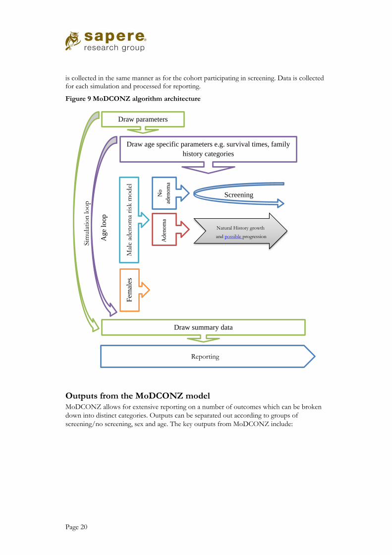
Figure 9 below shows the high level architecture of the MoDCONZ algorithm. A set of parameters are drawn for each simulation loop and used for the modelling of each individual in the population. For each age the population is processed in four groups: for each gender the adenoma risk model (see Appendix 1) is applied to divide the cohort into those with and without a lifetime risk of developing adenomas. For those with no adenomas there is no base case, but the cohort is run through screening to determine the number of people eligible, the returned iFOBTs and the consequences, including false positives and colonoscopies. For those with adenomas, their natural history simulation models adenoma growth and potential progression into cancers and cancer deaths, and the base case for those with detected cancers
No adenoma
Small adenoma <10mm
Large adenoma ≥10mm
Bowel Cancer
Stage I
Stage II
Stage III
Stage IV
Page 20
is collected in the same manner as for the cohort participating in screening. Data is collected for each simulation and processed for reporting.
Figure 9 MoDCONZ algorithm architecture
Outputs from the MoDCONZ model MoDCONZ allows for extensive reporting on a number of outcomes which can be broken
down into distinct categories. Outputs can be separated out according to groups of
screening/no screening, sex and age. The key outputs from MoDCONZ include:
Sim
ula
tio
n lo
op
Draw parameters
Age
loop
Draw age specific parameters e.g. survival times, family
history categories
Fem
ales
Draw summary data
Reporting
Screening
Mal
e ad
eno
ma
risk
mo
del
Natural History growth
and possible progression
No
aden
om
a A
den
om
a

Page 21
• Incidence of bowel cancers by stage;
• Incidence of bowel cancer related deaths;
• Life years;
• Quality adjusted life years (QALYs);
• Number of FITs completed;
• Number of colonoscopies;
• Cost of screening;
• Cost offsets from screening.
2.2.2 Model calibration and validation The base microsimulation model addresses the sensitivity of the natural history parameters
through a Bayesian calibration with incidence and death data.
Bayesian calibration
The set of parameter vectors for the simulation are the output of a Bayesian calibration
process. The natural history model has many parameters that are not known constants. The
multiple sets of parameter vectors collectively represent the uncertainty of their values. By
looping the natural history model through a large number of parameter vectors, an
estimation of the credible intervals of the outcome of interest (e.g. number of cancers) can
be obtained by statistical measures of the resulting sample of values obtained for that
outcome.
Approximately, the Bayesian calibration involves finding the parameter sets that lead the
model outputs to match our observed calibration targets from the New Zealand cancer
register as well as possible. The resulting posterior set contains 100 parameter vectors. We
use a normal approximation based on the mean and variance to derive the uncertainty of
outcomes.
For a larger parameter set of 1000, the 95% approximate credible intervals are obtained by
locating the 2.5th and 97.5th percentiles of the outcome of interest.
2.2.3 Falling rates of bowel cancer mortality In New Zealand, and a number of other countries, the rates of bowel cancer mortality and
incidence have been falling for the last 30 years. Over the 20 years prior to 2005 the NZ
bowel cancer mortality rate for men decreased by 35 percent25. The MoDCONZ model
accounts for this decreasing trend in bowel cancer mortality and incidence through a
quadratic fit to underlying incidence. While this fits the observed data, this approach limits
the degree to which future extrapolation of incidence (and therefore screening impact) can
robustly be conducted.

Page 22
2.3 Screening intervention model We added a screening intervention model to MoDCONZ in order to estimate the benefits
and costs of bowel cancer screening. The screening intervention estimates the:
• earlier detection of bowel cancer and the resulting changes in bowel cancer mortality;
• costs of screening (including surveillance); and
• cost offsets from reduces treatment of cancer.
The screening intervention model is summarised in Figure 10 below. A number of steps are
modelled, from the proportion of the population invited through to the outcomes from
colonoscopies. The values used, and the underlying evidence base, for each step of the
intervention model is detailed in the following sections.
The screening steps in the model are as follows:
• Population for screening identified, based on invitation criteria, i.e. age;
• Most people who meet the criteria are invited and sent an iFOBT kit;
• Some patients return iFOBT that can be analysed;
• People notified of iFOBT result:
Positive tests are followed up with a call from the person’s general practitioner,
and the person is referred for colonoscopy;
Negative results are notified via mail to the participant and their GP, the person is
invited to screening in the next round (as long as they still meet the invitation
criteria).
• Invitation to colonoscopy for those with a positive iFOBT:
If cancer found, treatment is offered and the person leaves screening for treatment.
Early (Stage 1 or 2) cancers enter the colonoscopy surveillance program;
Adenomas are removed (in our model we assume all adenomas ≥3mm are
removed);
Intermediate and high risk patients, defined by the number and size of adenomas,
leave screening and enter colonoscopy surveillance;
Histology is performed on all adenomas and cancer found;
Low risk patients and those without adenomasi are invited to screening in the next
round.
i In the pilot, when those who had a colonoscopy and no adenomas were found, they were invited back to
screening in five years. In MoDCONZ we model the participants being invited back in two years. The difference is unlikely to have a significant effect on the result.

Page 23
Figure 10 Screening and surveillance intervention model schematic
2.4 Modelling specifications
2.4.1 Cohort We have modelled a cohort of patients from age 40 through to death, assuming a maximum
age of 111. Our cohort is notionally based on those born in 1957, a cohort of 56,552 people
(based on the number alive at age 44) made up of 27,832 males and 28,720 females. This
approach allows us to track a population through the entire duration of screening, i.e. from
first to last year of eligibility. This approach represents the steady state cost-effectiveness,
which may differ from the cost-effectiveness in the short term (since in the short term
screening is offered for the first time to those who are towards the end of the age band).
Cost and QALYs are calculated from the age of 50, i.e. the first year screening is offered.
2.4.2 Discounting As with all economic analyses, we discount future benefits back to today’s dollars. A
discount rate of 3.5 percent p.a. is applied to benefits and costs. 3.5 percent is the standard
discount rate applied by New Zealand’s pharmaceutical purchasing agency PHARMAC26 in
economic analysis, and facilitates comparability of results for this analysis with analyses for
other health interventions. The discount rate is a ‘real’ rate of return, i.e. inflation is
accounted for within the discount rate.
2.4.3 Proportion invited Nearly all of the population aged 50 – 74 in the Waitemata district were invited to take part
in screening and sent a iFOBT kit; however 4 percent were not invited. The reasons for not
being invited include:
• People opted out;
• Registered as already having bowel cancer and/or in surveillance;

Page 24
In our model, we assume that 96 percent of people in the eligible age range would be sent an
iFOBT kit.
2.4.4 iFOBT participation rate The New Zealand pilot provides information for two rounds of screening. In the base case
we assume the participation rate by age band will be the same for future rounds. We explore
scenarios using a range of participation rates, which will inform the value of programmes to
sustain or improve the participation rates.
We define iFOBT participation rate as the proportion of people sent an iFOBT kit that
return a kit that produces a result. Those who return a kit which cannot be analysed are
counted as not participating.
We have included three parameters in our model for iFOBT participation:
• New to screening, i.e. the first round;
• Participated in previous round;
• Did not participate in previous round.
We have assumed that in the steady state iFOBT participation for Maori will be the same as
for the whole population. While the participation rate for Maori was lower than the overall
population in the pilot, in the 2nd round of the pilot Maori had the highest rate of
participation among those who did not participate in the 1st round. If this trend of increased
participation for Maori continued then the participation rate for Maori will ultimately
converge with the overall population.
Participation based on the pilot The preliminary results of the pilot provide participation rates split by age group and
previous participation. For those new to screening, we use the rates reported by age groups
(reported as ‘new to screening’ Table 5 below). For those who have previously been invited
to screening, the participation rates are dependent on whether the individual participated in
the previous round.
In order to estimate the participation rate given participation in previous rounds, we applied
the observed ratio of increased participation. For example, for all age groups the
participation rate is 1.51 higher (83 percent compared with 55 percent) for those who have
previously participated compared with those participating in the first round. Applying this to
those aged 50 – 54 results in an estimated participation rate of 62 percent for those who
previously participated. For the age group 70 – 74 the participation rate in the pilot was 70
percent, applying a multiplier of 1.51 to estimate the participation rate for those who
previously participated would results in an estimate exceeding 100%; therefore in this case
we have assumed a participation rate of 95 percent.

Page 25
Table 5 Participation rates used in our model
Age group 50-54 55-59 60-64 65-69 70-74
New to screening 43% 49% 56% 64% 70%
Participated in previous
round
65% 73% 85% 95% 95%
Did not participate in
previous round
18% 21% 24% 27% 30%
Comparison with published analyses In the four cost-utility analyses we reviewed in detail, three included participation rates in the
base case. The rates were ~37 percent27 and 60 percent28,29. One analysis assumed 100
percent participation and varied the rate in the sensitivity analysis30. The published analyses
we reviewed used the same participation rates regardless of age or previous participation of
the individual (although one study assumed all invited would participate at least once29). It is
not surprising that the participation rates varied, since international experience shows a wide
range of participation.
Examples of participation rates changing over time with varying starting age for cohorts We have included our projected participation rates in order to illustrate the impact of using
our estimated participation rates. We include two scenarios to show the impact of starting
screening at different ages.
Example: starting with a cohort of age 50
Figure 11 below shows how the participation rate changes over time for a cohort with a
starting age of 50 (i.e. the base case for our analysis). The participation rate is 43 percent in
the first round and drops to the lowest participation rate of 36 percent in the 3rd round.
The participation rate rises steady to a maximum of 82 percent in the 13th round. The
average participation rate is 56 percent.

Page 26
Figure 11 Example of participation rates changing over time: starting with a cohort of
age 50
Example: starting with a cohort of age 60
Figure 12 below shows how the participation rate changes over time for a cohort with a
starting age of 60. The participation rate is 56 percent in the first round. The participation
rate rises steady to a maximum of 82 percent in the 9th round. The average participation rate
is 69 percent.
Figure 12 Example of participation rates changing over time: starting with a cohort of
age 60
2.5 Performance of iFOBT The performance of iFOBT, as with any test, is measured as sensitivity and specificity.
Sensitivity is the ability to correctly detect those with adenomas or cancers. Specificity is the
0%
20%
40%
60%
80%
100%
150-54
350-54
555-59
760-64
965-69
1170-74
1370-74
Par
tici
pat
ion
rat
e, p
er
rou
nd
Screening round and age band of cohort
0%
20%
40%
60%
80%
100%
160-64
360-64
565-69
770-74
Par
tici
pat
ion
rat
e, p
er
rou
nd
Screening round and age band of cohort
Page 27
ability to correctly identify those without either adenomas or cancers. The sensitivity and
specificity, along with the prevalence, determine the positive predictive values, i.e. the likely
hood that someone with a positive FIT has an adenoma or cancer.
2.5.1 Data source for iFOBT performance Our approach to determining the performance of iFOBT had two elements. Firstly we used
studies where all participants received a colonoscopy (as a gold standard investigation) to
determine the sensitivity and specificity of iFOBT at a given cut-off. Secondly we used the
results of the pilot to infer how the sensitivity and specificity change for different cut-off
levels.
Evidence for sensitivity and specificity Our search revealed four studies that reported on the sensitivity and specificity of iFOBT
where all subjects were given a colonoscopy to confirm whether they had adenomas or
cancer.
We used the results of a large Japanese study, reported by Morikawa et al,31 to form the basis
of the estimates in our analysis. We used this study as the basis for our estimates for
sensitivity and specificity because of the large sample size and detailed reporting. The large
sample makes for more robust estimates for the less common finding of cancers. Even in
this large study only 81 cancers were detected. The second largest study we reviewed33 only
detected 8 cancers. None of the other three studies we reviewed included estimates of
sensitivity and specificity for non-advanced adenoma or the difference stages of cancers.
Comparison of Morikawa et al with other studies.
We compared the sensitivity and specificity values reported by Morikawa et al with results
from three other studies. The results are similar in all four cases, although the sensitivity and
specificity reported by Morikawa tend to be a little lower than the other studies.
The comparison has a number of limitations, which include the different countries, age
bands, brand of iFOBT test used and the definition of advanced adenoma. Despite these
limitations, the comparison gives us confidence that the sensitivity and specificity values
reported by Morikawa et al provide the best available basis for our model.
Table 6 summarises the comparison of the sensitivity and specificity values. Where a range of
results are reported we have taken those that are most comparable with Morikawa and the
pilot; e.g. a single iFOBT test and using a cut-off of 100 ngHb/ml buffer.
Further details of the Japanese study are included in the following section. Details of the
other studies are detailed in Appendix 2 (details of iFOBT performance).

Page 28
Table 6 Comparison of sensitivity and specificity of a single iFOBT test in asymptomatic population
Country, lead
Author
Detecting advanced Adenoma* Detecting cancer
Brand Positivity Population
Sensitivity Specificity Sensitivity Specificity
Japan
Morikawa31
22.8
(19.4 – 26.2)†
95.1†
(94.8 – 95.1) †
65.8
(55.4 – 76.3)
94.6
(94.3 – 94.9)
Magstream 1000
5.6% 21,805 patients
Average age of 48.2 years
1983 and 2002
Korea
Park32
23.7
(13.6 – 36.6)
94.0
(91.9 – 95.6)
69.2
(38.6 – 90.9)
93.7
(91.7 – 95.3)
OC sensor NR 770 patients
Aged 50 – 74
2007 to 2008
Amsterdam
de
Wijkerslooth33
29
(21- 39)
97
(95 - 98)
75
(36-96)
95
(93 - 96)
OC sensor 6% 1,256 patients
Aged 50 – 74
2009 to 2010
Germany
Brenner34 NR NR 73.3
(NR)
95.5
(NR)
OC sensor NR 2,235 patients
Aged 50 –79
2005 - 2009 † Morikawa: The 95% CI for Advanced adenoma were not reported, we assumed the same range as for adenoma ≥ 10 mm excluding high-grade dysplasia as reported in Morikawa 2005. The specificity was not reported, the values in the table in below refer to the specificity for advanced neoplasia (i.e. includes cancers) *Advanced adenoma defined different for each of the studies, Morikawa - adenomas with diameters of ≥ 10 mm (Reported in the follow up 2007 publication)
Park - tubular adenomas with diameters of ≥ 10 mm, or to tubulovillous or villous adenomas, or those with high-grade dysplasia regardless of size. de Wijkerslooth - adenoma ≥ 10 mm, an adenoma with villous histology ( ≥ 25 % villous), and / or an adenoma with high-grade dysplasia
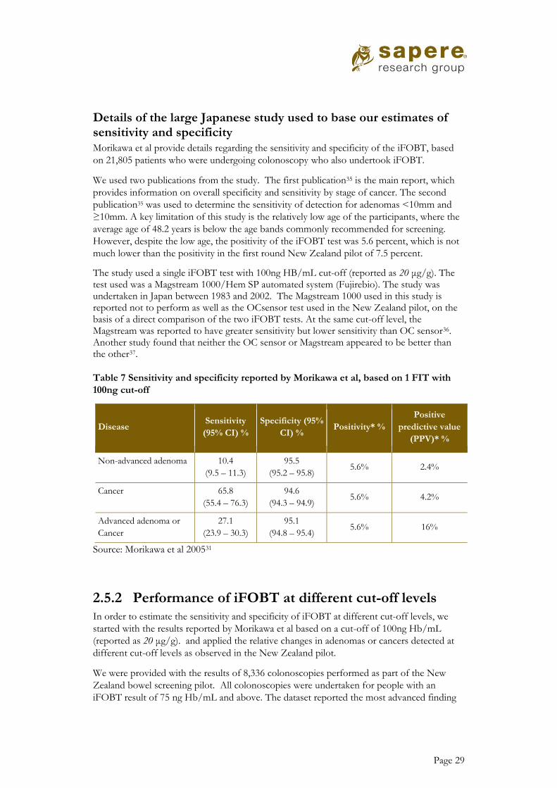
Page 29
Details of the large Japanese study used to base our estimates of sensitivity and specificity Morikawa et al provide details regarding the sensitivity and specificity of the iFOBT, based
on 21,805 patients who were undergoing colonoscopy who also undertook iFOBT.
We used two publications from the study. The first publication35 is the main report, which
provides information on overall specificity and sensitivity by stage of cancer. The second
publication35 was used to determine the sensitivity of detection for adenomas <10mm and
≥10mm. A key limitation of this study is the relatively low age of the participants, where the
average age of 48.2 years is below the age bands commonly recommended for screening.
However, despite the low age, the positivity of the iFOBT test was 5.6 percent, which is not
much lower than the positivity in the first round New Zealand pilot of 7.5 percent.
The study used a single iFOBT test with 100ng HB/mL cut-off (reported as 20 μg/g). The test used was a Magstream 1000/Hem SP automated system (Fujirebio). The study was undertaken in Japan between 1983 and 2002. The Magstream 1000 used in this study is reported not to perform as well as the OCsensor test used in the New Zealand pilot, on the basis of a direct comparison of the two iFOBT tests. At the same cut-off level, the Magstream was reported to have greater sensitivity but lower sensitivity than OC sensor36. Another study found that neither the OC sensor or Magstream appeared to be better than the other37.
Table 7 Sensitivity and specificity reported by Morikawa et al, based on 1 FIT with
100ng cut-off
Disease Sensitivity
(95% CI) %
Specificity (95%
CI) % Positivity* %
Positive
predictive value
(PPV)* %
Non-advanced adenoma 10.4
(9.5 – 11.3)
95.5
(95.2 – 95.8) 5.6% 2.4%
Cancer 65.8
(55.4 – 76.3)
94.6
(94.3 – 94.9) 5.6% 4.2%
Advanced adenoma or
Cancer
27.1
(23.9 – 30.3)
95.1
(94.8 – 95.4) 5.6% 16%
Source: Morikawa et al 200531
2.5.2 Performance of iFOBT at different cut-off levels In order to estimate the sensitivity and specificity of iFOBT at different cut-off levels, we
started with the results reported by Morikawa et al based on a cut-off of 100ng Hb/mL
(reported as 20 μg/g). and applied the relative changes in adenomas or cancers detected at
different cut-off levels as observed in the New Zealand pilot.
We were provided with the results of 8,336 colonoscopies performed as part of the New
Zealand bowel screening pilot. All colonoscopies were undertaken for people with an
iFOBT result of 75 ng Hb/mL and above. The dataset reported the most advanced finding

Page 30
(i.e. most advanced cancer or largest adenoma) and the ng HB/mL level of the FIT. This
allows us to estimate how many adenomas or cancer may have been detected at different cut-
off levels.
Using a cut-off of 200 instead of 75 ng Hb/mL would result in 46% fewer positive iFOBT
results; i.e. a fall in positivity from 6.8 percent to 3.7 percent. There would be a reduction in
all findings, from no adenomas to advanced cancers, shown in Figure 13 below.
PPV for cancers increases at higher cut-off, i.e. although fewer cancers are found, a positive
FIT is more likely to mean the person has a cancer. The proportion of people with positive
FIT that have bowel cancer is estimated to be 3.5 percent and 5.5 percent at 75 and 200 ng
Hb/mL cut-off respectively. This is below the high level recommended in European
guidelines.
Figure 13 Comparison of the number of positive iFOBTs (FITs) at different cut-offs
2.5.3 Sensitivity and specificity values used in our analysis
The sensitivity of the iFOBT is greater for cancers than for adenomas. Further, the
sensitivity is greater for those with advanced cancer than early cancer. The estimated
sensitivity for early stage cancer (stage I or II) is 59.7 percent, compared with late stage
cancer (stage III or IV) with a sensitivity of 85.9 percent. The sensitivity for adenomas is
relatively low with a 7.7 percent and 25.2 percent sensitivity for small (< 10mm) and large
(>=10mm) adenomas respectively. The specificity is estimated to be 94.7%, that is a person
without an adenoma or cancer has a 5.3 percent chance of a positive iFOBT (i.e. false
positive).
In order to model the cost-effectiveness of screening using different iFOBT cut-off values,
we estimated the sensitivity and specificity at different cut-off values, which were then used
in our scenario analyses. Increasing the cut-off increases the specificity and decreases the
sensitivity, reducing both true and false positive results. The sensitivity and specificity values
0
3000
6000
9000
7515
20040
Nu
mb
er
of
po
siti
ve F
ITs
iFOBT cut-off
Cancer stage III or IV
Cancer stage I or II
Adenoma >=10mm
Adenoma<10mm
No adenoma or cancer
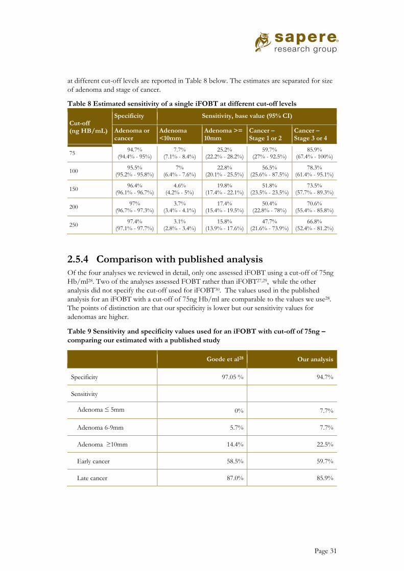
Page 31
at different cut-off levels are reported in Table 8 below. The estimates are separated for size
of adenoma and stage of cancer.
Table 8 Estimated sensitivity of a single iFOBT at different cut-off levels
Cut-off (ng HB/mL)
Specificity Sensitivity, base value (95% CI)
Adenoma or cancer
Adenoma <10mm
Adenoma >= 10mm
Cancer – Stage 1 or 2
Cancer – Stage 3 or 4
75 94.7%
(94.4% - 95%) 7.7%
(7.1% - 8.4%) 25.2%
(22.2% - 28.2%) 59.7%
(27% - 92.5%) 85.9%
(67.4% - 100%)
100 95.5%
(95.2% - 95.8%) 7%
(6.4% - 7.6%) 22.8%
(20.1% - 25.5%) 56.5%
(25.6% - 87.5%) 78.3%
(61.4% - 95.1%)
150 96.4%
(96.1% - 96.7%) 4.6%
(4.2% - 5%) 19.8%
(17.4% - 22.1%) 51.8%
(23.5% - 23.5%) 73.5%
(57.7% - 89.3%)
200 97%
(96.7% - 97.3%) 3.7%
(3.4% - 4.1%) 17.4%
(15.4% - 19.5%) 50.4%
(22.8% - 78%) 70.6%
(55.4% - 85.8%)
250 97.4%
(97.1% - 97.7%) 3.1%
(2.8% - 3.4%) 15.8%
(13.9% - 17.6%) 47.7%
(21.6% - 73.9%) 66.8%
(52.4% - 81.2%)
2.5.4 Comparison with published analysis Of the four analyses we reviewed in detail, only one assessed iFOBT using a cut-off of 75ng
Hb/ml28. Two of the analyses assessed FOBT rather than iFOBT27,29, while the other
analysis did not specify the cut-off used for iFOBT30. The values used in the published
analysis for an iFOBT with a cut-off of 75ng Hb/ml are comparable to the values we use28.
The points of distinction are that our specificity is lower but our sensitivity values for
adenomas are higher.
Table 9 Sensitivity and specificity values used for an iFOBT with cut-off of 75ng –
comparing our estimated with a published study
Goede et al28 Our analysis
Specificity 97.05 % 94.7%
Sensitivity
Adenoma ≤ 5mm 0% 7.7%
Adenoma 6-9mm 5.7% 7.7%
Adenoma ≥10mm 14.4% 22.5%
Early cancer 58.5% 59.7%
Late cancer 87.0% 85.9%

Page 32
2.6 Colonoscopy In this section we report the values and rationale for the following colonoscopy related
inputs:
• Rate of successful colonoscopy;
• Accuracy of colonoscopy (sensitivity and specificity);
• Complications from colonoscopy.
2.6.1 Rate of successful colonoscopy People with a positive iFOBT test are invited to have a colonoscopy. The rate of
colonoscopy is lower than 100%, since some people may not respond, while in some cases a
colonoscopy cannot successfully be performed.
In the pilot, 92 percent of people with a positive iFOBT had a successful colonoscopy. In
the first round of the pilot, the rate was slightly higher with 93% of those with a positive
iFOBT having a colonoscopy, compared with 90 percent in the second round.
In our model we have assumed the rate of successful colonoscopies to be the same as the
pilot, i.e. 92 percent. For the purposes of probabilistic sensitivity analysis, we estimate the
plausible 95% CI to be 90 to 95 percent.
The rate of successful colonoscopies is similar to those in other published cost-utility
analyses. Of the four published cost-utility analyses we reviewed in detail, three studies
included base case adherence rates of 8029, 85%28 and 92%27. One study assumed perfect
adherence in the base case and varied the adherence rates in the sensitivity analysis30.
2.6.2 Accuracy of colonoscopy Colonoscopy is the gold standard for detecting adenomas and cancers. However, sometimes
adenomas and cancers are missed during colonoscopy. For the purpose of our model we
have assumed specificity to be 100%, i.e. there are no cases of false positives, where an
adenoma or cancer is falsely thought to be present. However, sensitivity is less than 100
percent, since some adenomas and cancers may not be detected. As with FIT, the sensitivity
is better with more advanced/larger adenomas and more advanced cancers.
The sensitivity/performance of colonoscopy is better for distal rather than proximal
adenomas/cancers. The further the adenoma/cancer lies from the anus, the increased risk of
not being detected.
Of the four published cost-utility analyses we reviewed in detail,27,28,29,30 the sensitivities for
adenomas range from 75 to 95 percent, and the sensitivities for cancer ranged from 94 to 97
percent. Only one study29 differentiated the sensitivity between proximal and distal cancers.
The most commonly cited source of sensitivity for values was a systematic review of missed
rate of polyps by van Rijn et al38.

Page 33
The systematic review by van Rijn38 aimed to identify studies in which patients had
undergone two same-day colonoscopies with polypectomy. They also aimed to determine the
miss rate of optical colonoscopy independent of other diagnostic tests. When they searched
for studies between 1984 and 2005, they identified six cohorts including 465 patients that
met the criteria. The sensitivity was 97.9% for polyps ≥ 10mm (95% CI 92% - 99%) and
76.2% for polyps < 10mm (95% CI 72% - 81%)ii.
We identified a study of 12,487 patients in who had a new diagnosis of bowel cancer, who
had a colonoscopy in the previous three years39. This allowed the authors to determine the
rate of new or missed cancers. The study was based on patients in Ontario Canada with a
diagnosis of bowel cancer between April 1997 and March 2002. The rates of new or missed
cancers varied by location of bowel cancer, ranging from 5.9% for right sided cancer to 2.3
percent for rectal or sigmoid cancers. The overall rate of new or missed bowel cancers was
3.4% (430 of 12,487). This means the sensitivity is at least 96.6%, since it is only the number
of missed cancers which affects the sensitivity.
The specificity and sensitivity values for colonoscopy values used in our analysis are reported
in Table 10 below. The specificity value of 100 percent is based on common practice, as
reflected in the cost-utility analyses we reviewed. The sensitivity values by adenoma size are
based on the findings of the systematic review discussed above38. We have assumed the
sensitivity for cancer is the same as for adenoma’s ≥ 10mm; this assumption is based on the
close values reported for adenomas38 and cancers39. These values we use are similar to the
values used in the cost-utility analyses we reviewed.
Table 10 Performance of colonoscopy - values used in our analysis
Measure Value (95% CI)
Specificity 100%
Sensitivity: Adenoma
<10mm
76% (72% - 81%)
Sensitivity: Adenoma
≥ 10mm
98% (92% - 99%)
Sensitivity: Cancer 98% (92% - 99%)
Source: Sapere; based on values reported by van Rijn et al38
2.6.3 Complications from colonoscopies In the pilot about 1 percent of colonoscopies resulted in readmission. The most common
reasons for readmission were bleeding and perforation, representing approximately 60
percent and 11 percent of readmissions respectively. We have assumed 1 percent of
colonoscopies result in a readmission.
ii van Rijn et al reported the miss rate for adenomas 1-5mm and 5-9mm. We combined the number of missed
polps for all adenomas <10mm in order to get one value for miss rate.

Page 34
Comparison with published analyses Each of the analyses we reviewed in detail specified complications differently. It is therefore
difficult to make meaningful comparisons. Tappenden et al29 assumed a bleeding rate of 4.4
per 1,000 and perforation rates between 0.8 and 1.7 per 1,000. The lower perforation rate is
for colonoscopy without polypectomy. Goede et al28 assumed a complication rate of 2.4 per
1,000. Complications included were perforation, serosal burn, bleed with transfusion and
bleed without transfusion. Ladabaum et al30 assumed a major haemorrhage rate of 1.6 per
1,000 and a perforation rate of 0.85 per 1,000. Tran et al27 did not state the colonoscopy
complication rates used in their model, although they did reference the source.
2.7 Using QALYs to quantify health benefits Since the underlying principle of screening is to detect adenomas before they become cancers, and to detect cancers before they progress to more severe disease, health related quality of life (HRQoL) is inevitably an important consideration. We have quantified the changes in health outcomes using quality adjusted life years (QALYs). QALYs account for the time people spend in each health state and how the HRQoL differs for each health state.
Since New Zealand based quality of life data for bowel cancer patients is not currently
available, we have used published QALY values for our model. Our model includes different
QoL scores for the three phases of cancer, initial, continuing care and terminal phase. The
QoL in the initial phase was dependent on the stage at diagnosis, with more advanced cancer
being associated with a lower QoL score.
It was assumed that those without bowel cancer would have the QoL of the general
population. We based our estimate on study with 1,327 respondents from the general
population in New Zealand surveyed using the EQ-5D tool with the visual analogue score
technique40. The QoL was reported for seven different age bands. Given we are estimating
the QALYs in participants aged 50 and above, we estimated the average QoL for those aged
50 and above. We weighted the different scores by the proportion of the New Zealand
population in each age band as recorded in the latest census (2013). The QoL value for
those without bowel cancer is estimated to be 0.792.
Table 11 QoL for those without bowel cancer: population weights and QoL scores
used
Age band
Proportion of over 50
population* QoL score
50 -54 21% 0.822
55-64 35% 0.816
65-74 25% 0.796
75+ 19% 0.708
Total 100% 0.792
* Proportion of population taken from the 2013 censes as reported by Stats New Zealand

Page 35
The QoL scores for the initial phase of cancer were taken from the analyses reported by
Tappenden et al, based in turn on the results the survey reported by Ness et al. This study
surveyed 90 patients regarding 7 different bowel cancers health states. The QoL scores
ranged from 0.74 for ‘stage I rectal or stage I/II colon cancer’ and 0.25 for ‘stage IV rectal or colon
cancer’. These values are used for the stage I and stage IV respectively. We followed the
approach of Tappenden, estimating the QoL values for the in between cancer stages, Stage II
and Stage III as having QoL scores of 0.70 and 0.50 respectively.
While the QoL values derived by Ness should reflect the whole time spent in each health
state, i.e. each stage of bowel cancer, other studies suggest that over time patients QoL
improves (Ramsey et al)42 and that the QoL is close to the general population42,45, 46, 47.
Therefore we assume that in the continuing care phase, after the initial phase, patients QoL
improves to the level observed in the general population, i.e. 0.792.
In the terminal phase, the last year of life, the QoL score is assumed to be 0.25. This is based
on the assumption that the last year will be similar to being in stage IV of cancer.
If a patient lives for 1 year or less, the QoL score for the terminal phase is applied (0.25). If a
patient lives between 1 and 2 years, the QoL for the terminal phase is applied for the last
year of life, and the QoL from the initial phase is applied to the remainder of the life. If a
patient lives more than 2 years, Initial and terminal phase QoL scores are used for the first
and last year respectively, with the QoL score for continuing care applied to the time in
between.
The QoL scores for cancer are only applied to diagnosed cancer.
Table 12 QoL scores used in our model
Health State: stage of bowel
cancer
QoL score
(95% CI)
No diagnoses bowel cancer 0.792 (0.713 - 0.870)
Initial phase (first year
following diagnosis)
Stage I 0.74 (0.69 – 0.78)
Stage II 0.70 (0.65 – 0.75)
Stage III 0.50 (0.44 – 0.56)
Stage IV 0.25 (0.20-0.31)
Continuing care phase 0.792 (0.713 - 0.870)
Terminal phase – cancer (last
year of life)
0.25 (0.20-0.31)

Page 36
2.7.1 Comparison with values used in published analyses There is a very limited range of QoL scores used in published analyses of bowel screening. However, the application of those QoL scores is highly varied, which leads to varied QALY estimates from a given reduction in bowel cancer. QoL scores used in the literature vary from 0.25 to 0.90 for the different cancer stages, and from 0.91 to 1.0 for those without cancer. Table 13 below provides a brief summary of how three published studies applied QoL scores, further details are below. The QoL scores are based on two key studies. One study asks cancer patients to compare different health states, which requires patients to imagine what it would be like to be in each of the health state. While the second study asks patients how they feel given their current bowel cancer health state, although this study focused on the continuing care phase and is therefore limited to those who have a had diagnosis for at least a year.
Table 13 QoL scores used in published assessments
First author , year, country
Health state QoL (Utility score)
Comment
Tappenden 200429 UK
No known adenomas 0.91 Undiagnosed cancers assumed to have same QoL as no cancer. No cancer assumed to have some QoL decrement.
Cancer Dukes A* 0.74
Cancer Dukes B* 0.70
Cancer Dukes C* 0.50
Cancer Dukes D* 0.25
Goede 201328 Dutch
No known adenomas 1 QoL varies overtime within each health state
Cancer Dukes A* 0.74, 0.85, 0.25
Cancer Dukes B* 0.70, 0.85, 0.25
Cancer Dukes C* 0.50, 0.85, 0.25
Cancer Dukes D* 0.25
Ladabaum 201330 No known adenomas 1 (Assumed) Limited details provided. QoL between 37 – 60 months applied to entire time in health state
Localized colorectal cancer 0.90
Regional colorectal cancer 0.80
Distant colorectal cancer 0.76
*TNM staging is used in our analysis. Dukes A, B, C, and D have similar definitions as TNM stages I, II, III, and IV respectively
Tappenden et al29 noted that ‘evidence on the quality of life associated with colorectal cancer in scant and conflicting’ pg 60. Three studies were identified which attempted to measure quality of life associated with bowel cancer. Only one of these studies, Ness 199941, provided relevant information that could be used in their analysis. Ness et al surveyed 90 patients regarding 7 different bowel cancers health states. The QoL scores ranged from 0.74 for ‘stage I rectal or stage I/II colon cancer’ and 0.25 for ‘stage IV rectal or colon cancer’. These values where used by Tappenden et al for the Dukes A and Dukes D respectively, Tappenden estimated the QoL values for the in between cancer stages, Duke B and Dukes C as having QoL scores of 0.70 and 0.50 respectively. Tappenden at al assumed a

Page 37
QoL score of 0.91 for those without cancer (or with a cancer that isn’t diagnosed). 0.91 was based on separate study and determined by assuming the same QoL as for middle-aged individuals with one chronic health problem. QoL scores where applied for the duration of time spent in each health state. Ness et al41 derived their QoL scores using a standard gamble method. Each participant ended up producing QoL scores for five of the seven bowel cancer health states (only five per participant was used to shorten the interview time). Therefore, participants had to imagine the impact of being in a health state. Some of the patients would have experienced some of the health states as the participants were those we had colonoscopy with removal of adenomas. Goede et al 201328 used the MISCAN-colon model, which also use the QoL a values reported by Ness et al. However, they apply them differently. Goede et al modelled:
• QoL loss from bowel cancer is only included in the sensitivity analysis and not in the
base case.
• Values from Ness only applied during the first year of person being in each of stage of
cancer
• QoL in the year prior to death from bowel cancer is 0.25 (i.e. same as stage IV)
• QoL after 1 year of being in each stage, but prior to last year of life is 0.85 regardless
of stage of cancer [separate study reported]
• Quality of life score for being cancer free is 1, i.e. no decrement It is debatable whether to use the approach of varying quality of life during the time spent in each stage of cancer (as per MISCAN-colon), or using constant values (as per Tappenden). The former approach is likely to be more reflective of how QoL changes over time, but the later aligns with the source of the QoL scores as estimated by Ness et al. The increase in Quality of life after one year (but not in the year prior to death and not in stage IV) as modelled by MISCANZ is based on the findings of Ramsey et al42. Ramsey et al reported ‘After 3 years, respondents in all TNM stages of disease except Stage IV reported a relatively uniform and high quality of life.’ These findings are based on 173 respondents in the US who had a diagnosis of bowel cancer for at least 1 year, the stage of cancer at diagnosis varied across the respondents. The Health Utilities Index (HUI) Mark III was one of the tools used to measure QoL scores; individual dimensions are weighted according to values derived from the general Canadian population and summed to produce QoL score ranging from 0–1. The average quality of life score for all respondents was 0.85, this is the value used by Goede et al after 1 year of being in each stage, but prior to last year of life.
Ladabaum et al30 provide limited details on how QoL scores are used in their model.
However, they reference the Ramsey study as the source of the QoL scores. It appears
Ladabaum have taken the QoL scores as reported for respondents with 37 – 60 months
since diagnosis, based on the results of the HUI tool. For example, a QoL score of 0.76 was
applied to those with distant bowel cancer (i.e. stage IV), this not likely to represent most
patients with distant bowel cancer as the majority of patients diagnosed with distant bowel
cancer live for less than 1 year, with the QoL at the end of life being very poor. This method
may underestimate the impact of bowel cancer on patient’s quality of life, and overestimate
the QALY gains from bowel cancer screening.

Page 38
2.7.2 Quality of life scores in the literature Disability weights for the Global Burden of Disease 2013 study43
The Global Burden of Disease (GBD) study assesses health losses from diseases, injuries,
and risk factors using disability-adjusted life-years, which need a set of disability weights to
quantify health levels associated with nonfatal outcomes. The objective of this study was to
estimate disability weights for the GBD 2013 study.
Given the number and variety of health states included, there are limitations on the detail on
the health states. While the study does not look at the stage of bowel cancer, or even bowel
cancer itself, it does report on cancer in general. The QoL scores for cancer range from
0.431 for those in terminal phase without medication and 0.712 for diagnosis and primary
treatment. Further results are in Table 14 below.
Table 14 Disability weights for the Global Burden of Disease 2013 study - Cancer
health states
Health state Disability
weight QoL score (implied)
Cancer: Diagnosis and primary treatment 0.288 0.712
Cancer: Metastatic 0.451 0.549
Mastectomy 0.036 0.964
Stoma 0.095 0.905
Terminal phase: With medication (for cancers
and end-stage kidney or liver disease)
0.540 0.460
Terminal phase: Without medication (for
cancers and end-stage kidney or liver disease)
0.569 0.431
Source: Salomon et al 2011: Table 2
Färkkilä et al 2013 Health-related quality of life in colorectal cancer44
519 patients with bowel cancer responded to the survey. Patients were separated into 5
different health states. Three tools were used to measure QoL, include the EQ-5D (3 level).
In order to estimate QoL values for the general population, a UK tariff was applied to the
EQ-5d results. The QoL scores ranged from 0.850 for those in remission and 0.643 for
those receiving palliative care; further results are in Table 15 below. The QoL values for

Page 39
advanced bowel cancer are relatively high compared to the findings of Ness, this could be
due to relatively high time from metastases (16.1 for metastatic and 15.9 for palliative care
health states)
Table 15 QoL scores from Farkkila et al - EQ-5D 3L
Disease severity Health state QoL score
Local disease primary treatment
group
0.760
in rehabilitation 0.835
in remission 0.850
Advanced disease in metastatic disease 0.820
palliative care 0.643
2.7.3 Other quality of life studies There are a number of studies that assess the impact of bowel cancer on quality of life.
However, many of these studies do not report QoL scores that can be used to inform
QALYs. We have summarised some of these studies below, since they provide insights into
the impact of bowel cancer on QoL. These studies suggest that those who survive bowel
cancer tend to have similar QoL values to the general population.
21,802 patients surviving 12 to 36 months after a diagnosis of CRC and treated in the
National Health Service in England45 were included in this study. While the study uses the
EQ-5D tool it does not report the resulting QoL scores; this severely limits the usability of
the findings to inform our analysis. The results were “One or more generic health problems were
reported by 65% of respondents, with 10% of patients reporting problems in all five domains. The reporting
of problems was higher than in the general population and was most marked in those age less than 55 years.
Certain subgroups reported a higher number of problems, notably those with one or more other LTCs, those
with active or recurrent disease, those with a stoma, and those at the extremes of the age range (<55 and >
85 years).”
A study of 726 woman who had bowel cancer for an average of 7 years appear to report
health-related quality of life comparable with that of similarly aged women in the general
population46.
In a study of 309 bowel cancer patients that had survived one year from diagnosis, they
scored their physical, role, cognitive, and global health functioning only slightly worse than
the general population47.

Page 40
2.8 Cost of treating cancer There are significant costs to the health sector for treating bowel cancer and caring for those
with bowel cancer. Bowel cancer is estimated to cost the health sector an additional $46,000iii
per person diagnosed with bowel cancer. We base our estimates on work done by the
Department of Public Health, University of Otago, Wellington48. This research team used an
excess difference approach to estimate the additional cost incurred by those with bowel
cancer, compared with the general population.
2.8.1 Method for estimating costs The objective of the study was to determine health system expenditure on cancers by time
since diagnosis using data for an entire country. Patients included in the analyses were all
Usually Resident New Zealand cancer patients, with a prevalent cancer at any point in the
July 2006 to June 2011 period. The costs were taken from the following data sources:
• hospitalisations and inpatient procedures
• community laboratory tests;
• non-admitted patient events (e.g., outpatients);
• community pharmaceuticals dispensed (including patient contribution);
• general practice consultations
The established “excess” or “net” cost approach was used, whereby the expected health
system cost of a New Zealand citizens by sex and age group without the cancer diagnosis
was calculated, and then subtracted from the observed total health care costs of those with
bowel cancer. This approach avoids the need to classify in advance what counts as a specific
cancer-related cost.
Bowel cancer was defined as cancer recorded as colon, rectosigmoid, rectum, and anus and
anal canal. These cancers were identified using the ICD 10 codes C18 - C21.
The costs were broken into three time periods:
• 1st year following diagnosis
• Remission (time between 1 year and last 6 months)
• 6 months prior to death
The costs in the 1st year and remission differ by stage of cancer at diagnosis. Dukes staging
was used, and we have assumed that Dukes A, B, C, D have the same costs as TMN stages I,
II, III, and IV respectively. The costs in the 6 months prior to death are assumed to be the
same for all stages of cancer.
The costs were estimated by age bands for males and females. Cost were inflation adjusted
and reported in 2011 New Zealand dollars. We further inflation adjusted the study’s reported
figures to 2017 dollars. Figures were inflated up to 2015 based on the actual general inflation
iii Reported as $43,000 in 2011 dollars. Inflation adjusted to 2016 dollars.

Page 41
rate using the Reserve bank of New Zealand’s inflation calculator; to inflate to 2016 the
historical inflation rate of 2.5% p.a. was used.
2.8.2 Costs of treating bowel cancer The pattern of costs found by the Otago team is the same for male and females, although the
costs for males are approximately 15% higher. The majority of the costs are experienced in
the first 6 months following diagnosis, and the cost in the first 6 months varies significantly
by stage of bowel cancer at diagnosis; this can be seen in Figure 14 below. The cost of
treating bowel cancer is highest for those diagnosed with stage III cancer, with the cost 50%
higher than stage II and IV and over twice the cost of stage I.
Figure 14 Lifetime excess health care costs from bowel cancer, by stage of cancer and
time since diagnosis – females aged 60 - 69
The life time costs tend to be higher for those with a younger age of diagnosis. This trend is
shown in Figure 15 below. The trend of decreasing excess costs is seen in each of the three
time periods following diagnosis.
The reduction in initial costs with increasing age could be due to older patients being less
likely to receive treatments, if not being healthy enough for treatment and having less
potential benefit from treatment. The reduction in remission costs with increasing age is
likely due to the shorter life expectancy to accumulate costs. The reduction in end of life
costs (last 6 months) with increasing age is likely to be due to increased costs for older
people without bowel cancer.
$0
$25,000
$50,000
$75,000
$100,000
Sta
ge I
Sta
ge I
I
Sta
ge I
II
Sta
ge I
V
life
tim
e e
xcess
healt
h c
are
co
sts
of
bo
wel
can
cer
6 months prior to death
Remission
1 year following diagnosis
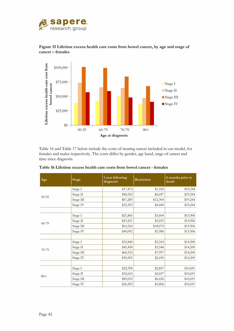
Page 42
Figure 15 Lifetime excess health care costs from bowel cancer, by age and stage of
cancer – females
Table 16 and Table 17 below include the costs of treating cancer included in our model, for
females and males respectively. The costs differ by gender, age band, stage of cancer and
time since diagnosis.
Table 16 Lifetime excess health care costs from bowel cancer - females
Age Stage 1 year following diagnosis
Remission 6 months prior to death
50-59
Stage I $17,472 $1,185 $19,244
Stage II $46,922 $6,047 $19,244
Stage III $67,285 $12,304 $19,244
Stage IV $32,303 $4,440 $19,244
60-79
Stage I $21,866 $3,604 $15,906
Stage II $43,431 $5,055 $15,906
Stage III $63,224 $18,074 $15,906
Stage IV $40,092 $1,986 $15,906
70-79
Stage I $32,840 $2,343 $14,200
Stage II $45,458 $3,548 $14,200
Stage III $60,332 $7,997 $14,200
Stage IV $30,502 $2,430 $14,200
80+
Stage I $22,598 $2,847 $10,691
Stage II $32,665 $2,697 $10,691
Stage III $49,052 $6,626 $10,691
Stage IV $26,202 $2,806 $10,691
$0
$25,000
$50,000
$75,000
$100,000
50-59 60-79 70-79 80+
Lif
eti
me e
xcess
healt
h c
are
co
st f
rom
b
ow
el
can
cer
Age at diagnosis
Stage I
Stage II
Stage III
Stage IV

Page 43
Table 17 Lifetime excess health care costs from bowel cancer - males
Age Stage 1 year following diagnosis
Remission 6 months prior to death
50-59
Stage I $25,097 $3,597 $19,244
Stage II $63,811 $8,158 $19,244
Stage III $71,676 $16,067 $19,244
Stage IV $42,267 $3,415 $19,244
60-79
Stage I $25,754 $2,443 $15,906
Stage II $53,956 $7,227 $15,906
Stage III $58,748 $14,823 $15,906
Stage IV $40,157 $4,630 $15,906
70-79
Stage I $33,651 $3,467 $14,200
Stage II $55,016 $6,134 $14,200
Stage III $59,439 $14,948 $14,200
Stage IV $36,584 $4,772 $14,200
80+
Stage I $34,660 $5,284 $10,691
Stage II $48,613 $2,514 $10,691
Stage III $44,713 $8,680 $10,691
Stage IV $35,657 $4,107 $10,691
2.8.3 Comparison with other estimates The most relevant comparisons are estimates based on New Zealand specific information,
since health system organisation and costs vary considerably across different countries.
Compared to the one other New Zealand study we identified, our costs are relatively high.
This is not surprising, since the other New Zealand study used a relatively conservative
approach.
Our estimates for cost of treating cancer are similar or lower than those reported
internationally and used in published cost-utility analyses. It is expected that some countries
will have higher costs for treating cancer, particularly where there are higher health care costs
in general. The pattern of costs for each of the stages of cancer is similar to what we have
used; except in stage IV cancer where there is significant variation in prices used. These
findings are further detailed in the sections below.
Page 44
Cost of cancer studies The Ministry of Health (MoH) has estimated the cost of bowel cancer to be NZ $28,000iv
per person, as reported in their Price of Cancer report49. This estimated cost is approximately
40% lower than the estimate we are using. There are a number differences in the methods
used to derive these estimates. The likely reason why the MoH’s estimate is lower is because
it includes only costs that were specifically coded as being due to cancer. Therefore this
result should be treated as a lower bound estimate48. The Price of Cancer report did not
include estimates by stage of cancer, so we cannot compare the relative costs by stage.
A study based in Ireland50 estimated the cost of treating bowel cancer by modelling the likely
costs experienced by those with bowel cancer. The estimated costs by stage in Ireland are
very similar to the cost we are using in our model, the only substantive difference being that
the cost of stage IV is estimated to be higher than in NZ. The authors concluded ‘The findings
illustrate the impact of biological agents on costs of cancer care. Therefore, this difference in stage IV is
likely to be due costs and usage of expensive biologic chemotherapy agents used in stage IV.
The average cost of bowel cancer, regardless of stage, is estimated to be much higher in
Ireland; this is likely to be due to more patients being diagnosed with later stage cancer and
the higher costs in Stage IV cancer.
A study based on Medicare data in the US51, reported the estimated cost of treating bowel
cancer to be $54,000v. This study used an excess cost approach (i.e. the same approach as the
costs used in the Otago analysis). The main difference in methods is that costs were
extrapolated out to 25 years and costs were discounted at a rate of 3.5%. While the overall
cost is similar to the NZ estimate, the cost by stage of cancer is very different. These US
estimates find that stage I has the highest cost, and stage IV has the lowest cost. This pattern
of cost by stage differs from all the other studies we identified. The cost of stage IV, is
estimated to be negative due to the short life expectancy associated with stage IV. We expect
the cost of treating Stage IV bowel cancer would currently higher, than in the patients
observed between 1996 and 2002, this increased cost is due to high cost biologic
chemotherapy treatments.
Cost used in other cost-utility analyses We have taken the estimates by stage of cancer from published cost-effectiveness studies
(converting them to 2016 NZ dollars) and compared them with our estimates. Two of the
four studies have values that are similar to the costs in our analysis. One study has similar
costs for early cancer and higher costs for late cancer. One study has much higher costs for
all stages, which may be attributable to being based on the US treatment regimens and US
costs (where US medical expenditure per person is among the highest in the world). This
comparison is shown in Figure 16 below.
iv Reported as $24,824 in 2008/09, we have inflation adjusted to 2016 cost
v Cost of treating bowel cancer reported to be $28,626 in 2006 USD, We converted to 2016 NZD

Page 45
Figure 16 Comparison of costs for treatment, by stage of bowel cancer
*The estimates for our analysis are based on the average for female and males, for those aged 60 – 79.
All four studies had stage I with the lowest cost, with increasing costs for Stage and II and
III. Two of the studies had stage IV costs that were lower than stage III costs. The studies
that have higher costs for stage IV likely include significant use of expensive biologic
chemotherapy agents.
The estimated costs by stage of bowel cancer reported in each of the studies are summarised
in Table 18 below. In order to convert the reported costs into comparable costs, we used the
exchange rate based on the year the costs were incurred in order to get New Zealand costs,
then we adjusted for inflation to get 2016 costs.
$0
$50,000
$100,000
$150,000
$200,000
$250,000
Sta
ge I
Sta
ge I
I
Sta
ge I
II
Sta
ge I
V
Est
imate
d l
ifeti
me c
ost
of
can
cer,
N
ZD
2016 Estimates in our Analysis*
Tappenden 2004 (UK)
Goede 2013 (Dutch)
Tran 2011 (Australia)
Ladabaum 2013 (US)

Page 46
Table 18 Cost of treating cancers used in published cost-effectiveness analyses
First author , year Stage of cancer Cost as reported Cost adjusted to 2016 NZD
Tappenden 200429 (UK)
Dukes A £8,299 $30,054
Dukes B £14,442 $52,299
Dukes C £19,076 $69,080
Dukes D £11,945 $43,257
Goede 201328 (Dutch)
I €25,540 $43,214
II €30,440 $51,505
III €34,240 $57,935
IV €35,940 $60,811
Tran 201127 (Australian)
I $34,337 $47,754
II $53,487 $74,386
III $79,924 $111,153
IV $71,156 $98,959
Ladabaum 201330* (US)
Local $90,672 $140,407
Regional $110,389 $170,938
Distal $134,286 $207,943
*Ladabaum included cost per year of continuing care for local and regional cancers. For the purposes of this comparison, we assumed 5 and 3 years of continuing care for local and regional cancers respectively

Page 47
2.9 Cost of screening Data on the cost of screening for the purpose of cost effectiveness analysis were derived as
part of a more comprehensive report on the cost of the Waitemata pilot, a companion report
to the present one. Some of the outputs were summarised differently in order to be suitable
for use with the MoDCONZ model.
Table 19 Screening costs
Cost Population Value
Mailout costs Eligible for screening $22.92
iFOBT analysis and reporting costs Participating in screening
• negative $18.73
• positive $111.45
Colonoscopy, by type Undergoing colonoscopies (positive iFOBTs and surveillance)
• In-house salaried /local anaesthetic $260.59
• In-house - private contractor/local anaesthetic
$487.51
• In-house salaried /general anaesthetic
$1,139.01
• private $1,019.66
• CT $427.75
Weighted average $754.92
Histology All samples collected at colonoscopy
$937.14
Re-admission following colonoscopy $5,172
Source: Sapere estimates, based on Sapere costing report of the pilot

Page 48
2.9.1 Cost of colonoscopy complications
We have based the costs of readmission on the average in-patient admission costs for
overnight admission in New Zealand.
We have used information published by the Ministry of Health to estimate the cost of an
admission for colonoscopy. MoH report the average cost-weights for Colonoscopy with or
without Catastrophic or Severe Complications as 1.91 and 1.00 respectively52. Using the
2014/15 cost weight of $4,681.9752 results in the following average costs:
• Colonoscopy with Catastrophic or Severe Complication: $8,947
• Colonoscopy without Catastrophic or Severe Complication: $4,705
We have assumed those colonoscopies resulting in a perforation to be associated in the more
expensive stay and the rest of the readmissions being associated with the less expensive stay.
Given approximately 11% of readmissions in the pilot were due to perforation, our
estimated cost for readmission is $5,172.
2.10 Modelling uncertainty There are three sources of uncertainty which can affect the results of this analysis, the sources are:
• structural uncertainty;
• choice of data sources; and
• parameter uncertainty53.
Structural uncertainty Structural uncertainty relates to the uncertainty due the structure of the model. This includes which health states are included in the model, and how pathways of care are represented. We have attempted to minimise structural uncertainty by modelling the model of care to closely align with New Zealand experience.
Choice of data sources The choice of data sources affects the inputs used in the model. For each model parameter we have searched for the most appropriate input, with consideration given to the quality of evidence and the applicability to the New Zealand setting.
In order to determine the impact of data sources, we include scenario analyses using alternative data values when there is more than one source that is a good match for the model. For example, we consider scenarios with varying participation rates.
Parameter uncertainty Each parameter (input) included in the MoDCoNZ model is associated with uncertainty. Sensitivity analysis is used to quantify the impact of parameter uncertainty. The base microsimulation model addresses the sensitivity of the natural history parameters through the Bayesian calibration with incidence and death data. The screening intervention model
Page 49
introduces a new set of parameters related to the decision points for each individual proceeding through the screening program and the performance of FITs. We incorporate probabilistic sensitivity analysis of these screening parameters into the MoDCoNZ screening model by performing a random draw on the distributions for these screening parameters at the same time as the draw of natural history parameters for each simulation run over the cohort of individuals.
Probabilistic sensitivity analysis (PSA) runs the model many times, with each run using a different set of values for each of the parameters. This creates a range of results which represents the uncertainty of the parameters. The values for each of the parameters for each run are based on the distribution for each parameter; with each distribution based on the best available evidence. PSA is the preferred method for addressing parameter uncertainty by the UK’s National Institute for Health Care and Excellence (NICE)53.
We derived alpha and beta parameters for a beta distribution for each screening parameter
from known or estimated 95% confidence intervals. For each simulation the parameters are
randomly drawn from the beta distributions, with the exception of iFOBT sensitivities. It is
assumed that iFOBT sensitivities are correlated, i.e. a higher degree of sensitivity to large
adenomas implies a higher sensitivity to cancers, and so on. The iFOBT sensitivities are
correlated by randomly drawing a percentile from a beta distribution, and determining the
parameter value for that percentile using each parameter’s beta distribution.

Page 50
3. Summary of assumptions
The inputs in the model are summarised in the tables below. The distributions listed are used
in the probabilistic sensitivity analysis; where no distribution is listed then the single value is
used.
Table 20 Parameter inputs – screening parameters
Parameter Mean (95% CI)
Screening
Proportion invited 96% (94% - 98%)
iFOBT Participation, new to screening Age dependent range:
43% to 70%
iFOBT Participation, participated in previous round Age dependent range:
65% to 95%
iFOBT Participation, did not participate in previous round Age dependent range:
18% to 30%
iFOBT sensitivity Adenoma < 10mm 7.7% (7.1% - 8.4%)
iFOBT sensitivity Adenoma ≥ 10mm 25.2% (22.2% - 28.2%)
iFOBT Sensitivity Stage 1&2 cancer 59.7% (27% - 92.5%)
iFOBT Sensitivity Stage 3&4 cancer 85.9% (67.4% - 100%)
iFOBT Specificity 94.7% (94.4% - 95%)
Rate of successful colonoscopy 92.5% (90-95%)
Colonoscopy specificity 100%
Colonoscopy sensitivity: Adenoma <10mm 76% (72% - 81%)
Colonoscopy sensitivity: Adenoma ≥ 10mm 98% (92% - 99%)
Colonoscopy sensitivity: Cancer 98% (92% - 99%)
Colonoscopy: Probability of complication resulting in re-
admission
1% (0.9% - 1.1%)
Quality of life
No diagnoses bowel cancer 0.792 (0.713 – 0.870)
Initial phase (first year following diagnosis)

Page 51
Stage I 0.74 (0.69 – 0.78)
Stage II 0.70 (0.65 – 0.75)
Stage III 0.50 (0.44 – 0.56)
Stage IV 0.25 (0.20-0.31)
Continuing care phase 0.792 (0.713 – 0.870)
Terminal phase – cancer (last year of life) 0.25 (0.20-0.31)
Cost of treating cancer (unweighted average by stage)
Treatment cost: Stage I $44,849
Treatment cost: Stage II $68,917
Treatment cost: Stage III $86,759
Treatment cost: Stage IV $54,054
Cost of screening
Eligible to receive a mail out $22.92 ($19.29 – $24.73)
Return iFOBT- negative results $18.73 ($15.54 – $20.30)
Return iFOBT - positive results $111.45 ($91.60 – $121.19)
Colonoscopy – mode weighted average $754.92 ($639.12 - $813.08)
Histology of samples collected at colonoscopy $937.14 ($793.38 -$1009.34)
Re-admission following colonoscopy $5,172 ($4,655 - $5,689)
Page 52
4. Reduction in cancers and cancer related deaths
Bowel cancer screening is estimated to results in the following benefits for the entire cohort
offered screening, up to the age of 84:
• 35 percent reduction in people with bowel cancer
• 45 percent reduction in bowel cancer deaths
4.1 Reduction in cancers In the base case we estimate there would be 4,921 bowel cancers diagnosed for those in the
cohort (counting cancer up to the age of 84) , i.e. 8.7 percent of the cohort who are alive at
age 44vi. With bowel cancer screening the cancers diagnosed are estimated to reduce to 3,183,
i.e. 5.6 percent of the cohort. The number needed to invite to screening to avoid a cancer is
33.
Screening results in a temporary increase in the diagnoses of cancers. In the first year of
screening there are an estimated 10 additional cancers detected. This is due to some people
having un-diagnosed cancers that are detected earlier due to screening. However, after the
first four years of screening the number of diagnoses in the screening arm is lower for any
given age; with the difference increasing with time. These results are shown in Figure 17
below, where the dotted red line represents the reduced number of people diagnosed with
cancer, compared with the solid blue line that shows the number diagnosed with cancer in
the base case (i.e. the absence of screening).
At the end of screening, there is a temporary drop in the number of people diagnosed with
cancer in the screening group. This drop is due to no longer actively looking for cancers. The
drop is illustrated in Figure 17 below by the drop in the dashed red line at age 75.
The number of diagnoses each year increase with age, until about age 80 when it starts to
decline. The number of diagnoses for those aged 80 is over four times higher for those aged
50. Therefore the greatest reduction in cancers is in those around the age of 80. While
screening only runs until age 75, the reduction in diagnosed cancers extends beyond the age
of 75 due to the prevention of cancers from the removal of adenomas.
vi Based in a cohort of 56,552

Page 53
Figure 17 Diagnoses of cancers age of diagnosis - cohort followed to age 84 - whole
population
Source: MoDCoNZ
4.2 Reduction in cancer deaths In the base case we estimate there would be 2,176 people who die from bowel cancer, i.e. 3.8
percent of the cohortvi (This aligns closely with the figure that 4.2 percentvii of people who
died in 2013 in New Zealand died from bowel cancer54). With bowel cancer screening the
number of people diagnosed with cancer would reduce to 1,196, i.e. 2.1 percent of the
cohort. The number needed to invite to screening to avoid a cancer deaths is 58 i.e. 1 in 58
people invited will avoided having a bowel cancer death.
The age profile of cancer deaths, and the reduction due to screening, is similar to the age
profile for cancers diagnosed. The cancer deaths by age for the base case and for screening
are shown in Figure 18 below.
vii In 2013, 1252 people had their cause of death recorded as bowel cancer (based on ICD codes C18 – C20, this
represents 4.2 percent of the 29,636 deaths recorded in 2013. Figures based on Ministry of Health’s provisional statistics.
0
50
100
150
200
250
40 45 50 55 60 65 70 75 80
Can
cers
dia
gno
sed
pe
r ye
ar
Age of diagnosis
Base Age 50 to 74, iFOBT cutoff 75ng

Page 54
Figure 18 Cancer deaths by age of death - cohort followed to age 84 – whole
population
Source: MoDCoNZ
4.3 Estimated impact for Maori Bowel cancer screening in the Maori population is estimated to results in in the following
benefits for the entire cohort offered screening:
• 34 percent reduction in people with bowel cancer
• 42 percent reduction in bowel cancer deaths
Although the relative reduction is the same for Maori and for the whole population, the
absolute number of cancers avoided per person invited is fewer for Maori, while the number
of cancer deaths avoided per person invited is the slightly higher for Maori and the whole
population. The reduced number of cancers avoided is due to a lower rate of bowel cancer in
Maori. The number needed to invite to screening to avoid a cancer is 39, a fifth more than
for the whole population. The number needed to invite to screening to avoid a cancer death
is 53, lower than the whole population result of 58.
The reduction in cancers and cancer deaths is similar for Maori and the whole population.
While more Maori have to be invited to screening to avoid a cancer, the number needed to
invite to avoid a bowel cancer death is similar across the whole population. We interpret this
as due to Maori having lower rates of bowel cancer, but similar rates of bowel cancer deaths.
0
20
40
60
80
100
120
140
45 50 55 60 65 70 75 80
Nu
mb
er
of
de
ath
s p
er
year
Age of diagnosis
Base Age 50 to 74, iFOBT cutoff 75ng

Page 55
5. Cost effectiveness results
5.1 Cohort The results presented in this section are based on following the cohort modelled in
MoDCONZ from the age of forty through to death, with a maximum age of 111. This
means that our cost effectiveness estimates are based upon following a cohort through their
entire experience of screening, rather than on the basis of a whole, changing, population over
a notional period of time. In effect, our analysis reflects the underlying steady state impact
of screening, rather than the simulating the absolute number of events which a screening
programme would encounter over a given time period.
5.2 National generalisation of the pilot In the previous sections of this report we have reported the components of the cost-utility
results. In this section we combine the components to estimate the cost per QALY, i.e. the
cost-effectiveness ratio. Further, we report the uncertainty of the results using probabilistic
and univariate analysis.
If bowel cancer screening was rolled out nationally in New Zealand in the same way that it
was undertaken in the pilot, it is estimated to dominate no screening; i.e. be cost saving with
QALY gains. The comparison of the outcomes for screening and no screening are included
in Table 21 below.
Our best estimate of the cost-per QALY for this scenario is -$1,344, i.e. cost saving with
health benefits. There is some uncertainty in the result: we estimate the cost per QALY to
fall in the range of -$5,786 to $4,850. This is a negative cost per QALY, which dominates all
other scenarios, since there is no tradeoff between cost and outcome.
Table 21 Cost-effectiveness of bowel cancer screening - based on national
generalisation of the Pilot – life time costs and benefits of the average person –
Whole population
Treatment Costs QALYs
Incremental Cost per
QALY
(95%CI) Costs
(95% CI)
QALYs
(95%CI)
No screening
$2,643 17.661 -$98
(-$627 - $219)
0.0730 (0.0451 - 0.1084)
Dominates* (-$5,786 -
$4,850) Screening $2,544 17.734
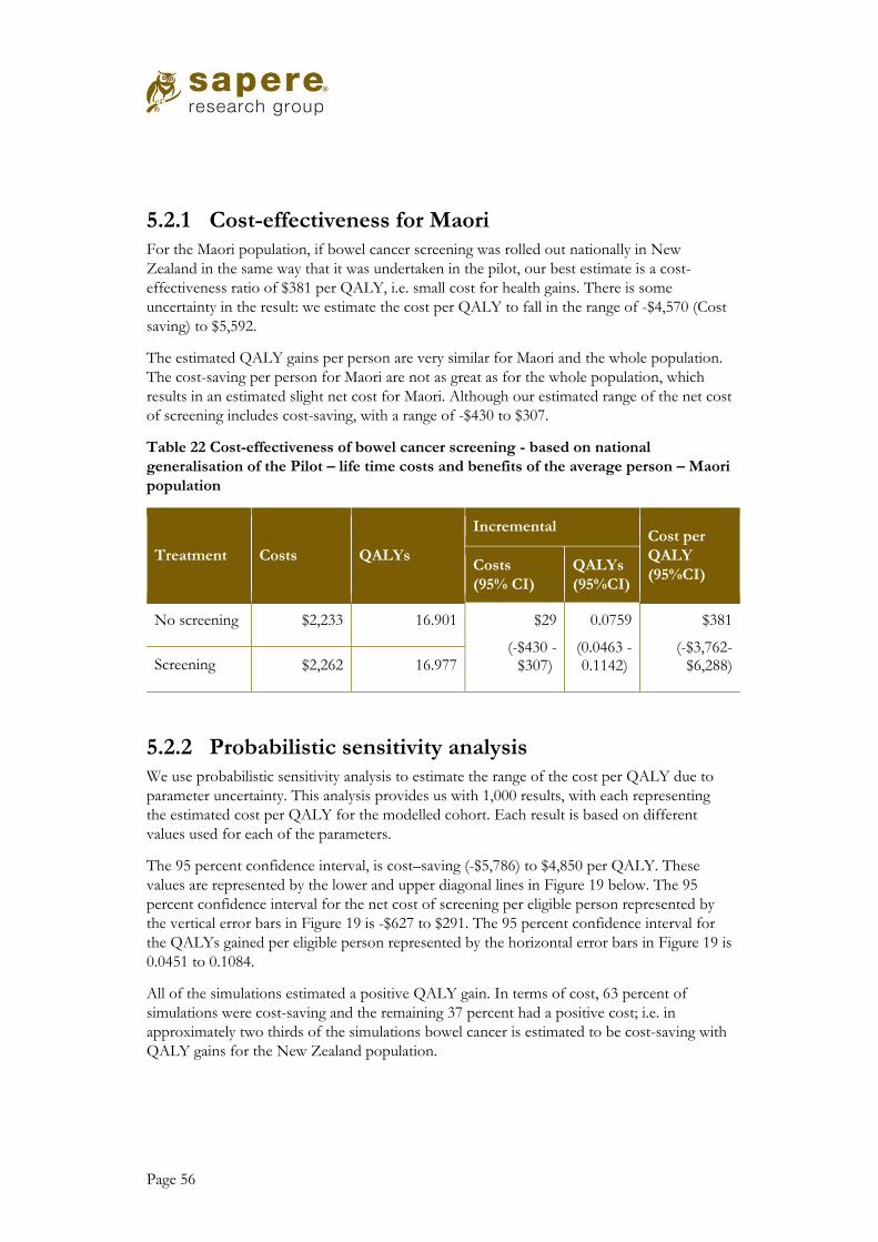
Page 56
5.2.1 Cost-effectiveness for Maori For the Maori population, if bowel cancer screening was rolled out nationally in New
Zealand in the same way that it was undertaken in the pilot, our best estimate is a cost-
effectiveness ratio of $381 per QALY, i.e. small cost for health gains. There is some
uncertainty in the result: we estimate the cost per QALY to fall in the range of -$4,570 (Cost
saving) to $5,592.
The estimated QALY gains per person are very similar for Maori and the whole population.
The cost-saving per person for Maori are not as great as for the whole population, which
results in an estimated slight net cost for Maori. Although our estimated range of the net cost
of screening includes cost-saving, with a range of -$430 to $307.
Table 22 Cost-effectiveness of bowel cancer screening - based on national
generalisation of the Pilot – life time costs and benefits of the average person – Maori
population
Treatment Costs QALYs
Incremental Cost per
QALY
(95%CI) Costs
(95% CI)
QALYs
(95%CI)
No screening $2,233 16.901 $29
(-$430 - $307)
0.0759 (0.0463 - 0.1142)
$381 (-$3,762-
$6,288) Screening $2,262 16.977
5.2.2 Probabilistic sensitivity analysis We use probabilistic sensitivity analysis to estimate the range of the cost per QALY due to
parameter uncertainty. This analysis provides us with 1,000 results, with each representing
the estimated cost per QALY for the modelled cohort. Each result is based on different
values used for each of the parameters.
The 95 percent confidence interval, is cost–saving (-$5,786) to $4,850 per QALY. These
values are represented by the lower and upper diagonal lines in Figure 19 below. The 95
percent confidence interval for the net cost of screening per eligible person represented by
the vertical error bars in Figure 19 is -$627 to $291. The 95 percent confidence interval for
the QALYs gained per eligible person represented by the horizontal error bars in Figure 19 is
0.0451 to 0.1084.
All of the simulations estimated a positive QALY gain. In terms of cost, 63 percent of
simulations were cost-saving and the remaining 37 percent had a positive cost; i.e. in
approximately two thirds of the simulations bowel cancer is estimated to be cost-saving with
QALY gains for the New Zealand population.

Page 57
Figure 19 Probabilistic sensitivity analysis: national rollout of the pilot
5.2.3 Univariate sensitivity analysis In order to understand what drives the uncertainty we have varied each parameter, or each
set of parameters, one by one. This analysis shows that our result is most sensitive to the
uncertainty in the natural history of bowel cancer.
The results of this analysis are shown in Figure 20 as a tornado diagram. The tornado
diagram makes it clear to see the parameters which create the largest uncertainty, as shown
by the wide bars for natural history. In this report we limit the number of parameters, or sets
of parameters, to the 10 that have the biggest impact on the results.
The uncertainty in the natural history of adenomas, and corresponding bowel cancers,
creates the largest uncertainty in the cost-effectiveness. The greater the number of
adenomas the more cost-effective bowel screening is. A low rate of adenoma results in a cost
per QALY of $4,138, and a high rate of adenomas results in a cost per QALY of -$6,799.
While the discount rate isn’t uncertain, the value chosen has a relatively large impact. A lower
discount rate improves the cost-effectiveness as the future benefits of screening are
discounted less. A discount rate of 0% results in a cost per QALY of -$4,692. A discount
rate of 5% results in a cost per QALY of -$5.
The discount rate applied during analysis and the cost of cancer also had an impact, although
a lesser one, upon cost effectiveness. In neither case does a plausible range of alternative
values reduce the cost effectiveness to a level at which screening would not be considered a
highly cost effective intervention.

Page 58
Figure 20 Univariate sensitivity analysis - Tornado diagram
5.3 Cost-effectiveness of different scenarios In this section we explore the impact on the cost-effectiveness of varying the following
parameters:
• iFOBT cut-off;
• age band for screening;
• iFOBT participation rate.
iFOBT cut-off and the age band for screening are two design parameters that can be
changed if bowel cancer screening is rolled out nationally. We have varied these parameters
to inform views on the different options for a national rollout. iFOBT participation rate was
included since it helps to inform the value of improving, or retaining, the participation rate
seen in the pilot.
5.3.1 iFOBT cut-off Bowel cancer screening is estimated to be less cost-effective at higher cut-off levels.
Increasing the iFOBT cut-off reduces the net savings and reduces the QALY gains.
Increasing the iFOBT cut-off from 75 to 250 results in a cost per QALY of $510, i.e. no
longer cost saving (although close to cost-saving). The cost per QALY for a range of iFOBT
cut-off values are shown in Table 23 below.
-$8,000 -$4,000 $0 $4,000
Natural history
Discount rate
Cost of treating cancer
Sensitivity and specificity - FIT and colonoscopy
FIT Participation
Colonoscopy cost
Invitation costs
FIT costs
Histology cost
QoL no cancer and remission
Cost per QALY
Low ICER
High ICER

Page 59
Table 23 Cost-effectiveness at differing FIT cut-off levels
FIT cut-off
(ng HB/mL) Cost per QALY
75 Dominates
100 Dominates
150 Dominates
200 $160
250 $510
The reduction in net savings and QALY gains at higher iFOBT cut-offs is shown in Figure
21 below. Increasing the iFOBT cut-off to 250ng results in a net cost of $34 compared with
a net saving of $98 in the base case. Increasing the iFOBT cut-off decreases the QALY gain
by 8 percent. The changes in the cost per QALY are driven by the changes in the net
savings.
Figure 21 Impact of iFOBT cut-off on, net savings, QALY gain and cost-effectiveness
-0.40
-0.20
-
0.20
0.40
0.60
0.80
1.00
1575
20100
30150
40200
50250
Ch
ange
re
lati
ve t
o b
ase
cas
e(1
= b
ase
cas
e)
Net Savings
QALY gain
Cost-effectiveness
µgHb/g fecesngHb/ml buffer

Page 60
Increasing the iFOBT cut-off decreases the number of positive iFOBT tests. This leads to
lower screening costs and reduced cost-offset; although the larger effect is a reduction in
cost-offsets which leads to a decrease in net savings (as shown in Figure 21 above).
Increasing the iFOBT cut-off reduces the number of adenomas and cancers detected; which
results in fewer cancers and cancer deaths avoided from screening. This reduction in cancers
and cancers deaths avoided is what drives the reduction in QALYs shown in Figure 21
above.
Using an iFOBT cut-off of 250ng results in a 24 percent reduction in cancers, compared
with a 35 percent reduction with a cut-off of 75ng (i.e. one third fewer cancers avoided than
when using the higher iFOBT-cut off). The estimated number of cancers with no screening
and screening using different iFOBT cut-offs is shown in Figure 22 below. The top line in
the figure below represents the number of cancers diagnosed without screening, by age. The
lines in the figure below represent the number of cancers with screening with an iFOBT cut-
off of either 75ng or 250ng, with 75ng iFOBT cut-off represented by lower line due to the
greater reduction in cancers.
Figure 22 Diagnoses of cancers by age of diagnosis - cohort followed to age 84 –
comparing different iFOBT cut-off values
The impact of using a higher iFOBT cut-off is smaller for the reduction in cancer deaths,
compared with cancers. Using a iFOBT cut-off of 250ng results in a 34 percent reduction in
cancer deaths, compared with a 45 percent reduction with a cut-off of 75 (i.e. a quarter fewer
cancer deaths avoided when using the higher iFOBT-cut off).
In this section we compared the sensitivity and specificity using different cut-off values of a
single iFOBT test. Another way to increase the performance of iFOBT is to perform
multiple tests. We have identified one study that reported that taking the highest values of
multiple iFOBT increased the sensitivity while decreasing the sensitivity; this pattern was
0
50
100
150
200
250
40 45 50 55 60 65 70 75 80
Can
cers
dia
gno
sed
pe
r ye
ar
Age of diagnosis
Base Age 50 to 74, iFOBT cutoff 75ng
Age 50 to 74, iFOBT cutoff 250ng

Page 61
consistent at different cut-off values55. However, we have not assessed the impact of
performing multiple tests, which could be an area for further research.
5.3.2 Age band for screening Using a narrower age band is more cost-effective, up to a point. Five of the six narrower age
bands we assessed resulted in increased cost-effectiveness. However, there is reduced
efficacy from screening when narrowing the age bands.
Using a narrower age band is usually more cost-effective because the efficacy of screening
reduces with each additional episode of screening. The reduction in efficacy is due to people
being less likely to have a cancer or adenoma if they have previously taken part in screening.
The reduction in QALY gains and increase in net savings from using narrower age bands are
shown in Figure 23 below. The most cost-effective age band is estimated to be 60-74.
Narrowing the age band to 60-74 increases the saving 69 percent and the decreases the
QALY gain by 5 percent; given the increase in net saving, the cost–effectiveness improves by
79 percent.
Figure 23 Impact of age band on, net savings, QALY gain and cost-effectiveness
Narrowing the age bands decreases the number of rounds people can participate in. This
leads to lower screening costs and reduced cost-offset; although the larger effect is a
reduction in screening costs which leads to a reduction in net costs (as shown in Figure 23
above).
Narrowing the age band reduces the number of adenomas and cancers detected; which
results in fewer cancers and cancer deaths avoided from screening. This reduction in cancers
and cancer deaths avoided is what drives the reduction in QALYs gained shown in Figure 23
above.
Using an age band of 60-74 results in a 28 percent reduction in cancers, compared with a 35
percent reduction with an age band of 50-74, i.e. a fifth of a reduction in the number of
cancers avoided when using a narrower age band. The estimated number of cancers with no
screening and screening using age bands is shown in Figure 24 below. The top line in the
figure below represents the number of cancers diagnosed without screening, by age. The
lower lines in the figure below represent the number of cancers with screening.
-
0.20
0.40
0.60
0.80
1.00
1.20
1.40
1.60
1.80
50-74 50 – 69 50 – 59 55-74 60-74 65-74
Ch
ange
re
lati
ve t
o b
ase
cas
e(1
= b
ase
cas
e)
Age band
Net savings
QALY gain
Cost effectiveness
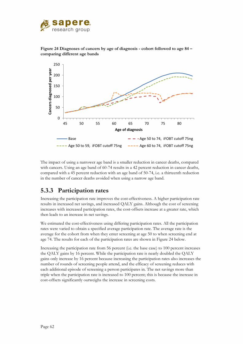
Page 62
Figure 24 Diagnoses of cancers by age of diagnosis - cohort followed to age 84 –
comparing different age bands
The impact of using a narrower age band is a smaller reduction in cancer deaths, compared
with cancers. Using an age band of 60-74 results in a 42 percent reduction in cancer deaths,
compared with a 45 percent reduction with an age band of 50-74, i.e. a thirteenth reduction
in the number of cancer deaths avoided when using a narrow age band.
5.3.3 Participation rates Increasing the participation rate improves the cost-effectiveness. A higher participation rate
results in increased net savings, and increased QALY gains. Although the cost of screening
increases with increased participation rates, the cost-offsets increase at a greater rate, which
then leads to an increase in net savings.
We estimated the cost-effectiveness using differing participation rates. All the participation
rates were varied to obtain a specified average participation rate. The average rate is the
average for the cohort from when they enter screening at age 50 to when screening end at
age 74. The results for each of the participation rates are shown in Figure 24 below.
Increasing the participation rate from 56 percent (i.e. the base case) to 100 percent increases
the QALY gains by 16 percent. While the participation rate is nearly doubled the QALY
gains only increase by 16 percent because increasing the participation rates also increases the
number of rounds of screening people attend, and the efficacy of screening reduces with
each additional episode of screening a person participates in. The net savings more than
triple when the participation rate is increased to 100 percent; this is because the increase in
cost-offsets significantly outweighs the increase in screening costs.
0
50
100
150
200
250
45 50 55 60 65 70 75 80
Can
cers
dia
gno
sed
pe
r ye
ar
Age of diagnosis
Base Age 50 to 74, iFOBT cutoff 75ng
Age 50 to 59, iFOBT cutoff 75ng Age 60 to 74, iFOBT cutoff 75ng

Page 63
Figure 25 Impact of age band on, net savings, QALY gain and cost-effectiveness
5.4 Comparison of results The cost-effectives results of bowel cancer screening compare very favourably with cost
effectiveness results both nationally and internationally. Many health interventions have a
positive cost-effectiveness, i.e. an increase in cost for improved health outcomes. However,
we estimate bowel cancer screening to be cost-saving with improved health outcomes. In
decision analysis terms, this is a highly attractive intervention.
5.4.1 Pharmaceutical funding in New Zealand The funding of pharmaceuticals (and some devices) in New Zealand is managed by
PHARMAC. PHARMAC have reported the average cost-effectiveness of the investments
they have made in each of the last four years. The cost-effectiveness ranges from $16,00056
to $45,00057 per QALYviii. These values represent the average for the investments made in
the year: the highest cost-per QALY invested in will be higher than these average values.
5.4.2 WHO recommendations The World Health Organisation (WHO) uses the following definitions of cost-effectiveness:
• Very cost-effective: less than GDP per capita;
• Cost effective: between 1 – 3 times GDP;
• Not cost effective: over 3 times GDP per capita.58
In 2015 New Zealand’s GDP per capita was $53,00059. Using the WHO definitions, bowel
cancer screening would be considered very cost-effective.
viii PHARMAC reports cost-effectiveness in terms of QALYs per million, which is the inverse of cost per QALY.
The average QALYs per million were reported be 22 and 61 in the 2011/12 and 2014/15 years respectively
-
0.50
1.00
1.50
2.00
2.50
56% 50% 80% 100%
Ch
ange
re
lati
ve t
o b
ase
cas
e(1
= b
ase
cas
e)
Participation rate - average
Net Savings
QALY gain
Cost-effectiveness

Page 64
6. Comparison of results with existing screening programmes
We reviewed published cost-effectiveness analyses and compared their results with our
analysis. There is significant variation in the assumptions and results of the analyses we
reviewed, however our result is within the range of the existing reported results from the
international literature.
The results of published analyses were summarised by Lansdorp-Vogelaar et al, reported as:
“All [32] studies found that colorectal cancer screening was cost-effective or even cost-saving compared with no
screening. However, the studies disagreed as to which screening method was most effective or had the best
incremental cost-effectiveness ratio for a given willingness to pay per life-year gained.”60 This finding was
based on an exhaustive review of publications between 1993 and 2009. There is significant
variation between the results, and the authors conclude it is difficult to determine the cause
of the variation as assessments with very similar assumptions have differing results.
There is limited analysis on the impact of screening on quality of life. Most of the analyses
report life years gained, rather than quality adjusted life years (QALYs) gained.
We undertook a detailed comparison of our model with four published analyses. We
identified analyses that were most relevant and had sufficient details reported in order to
make a meaningful comparison. Amongst these analyses there was a wide range in the
inputs, for example participation rates varied between 37% and 100%. There was also a wide
range in the results, from cost-saving to $53,000 per life year saved. A high level summary is
included in the following section, with further details included in Appendix 3.
6.1 Summary of individual cost-effectiveness analyses
We searched for cost-effectiveness analyses that met the following criteria
• FIT or iFOBT screening compared with no screening
• Report in detail in terms on basis for assumptions and results
We identified four studies meeting these criteria27,28,29,30. One of the studies had limited
details reported;27 however, we included this study because it is relatively recent, and
provides an interesting comparison with the Australian setting.
The most descriptive report we identified was by Tappenden et al,29 which appraised
screening options in the UK setting. The assessment is relatively similar to our analysis, with
key differences being the use of FOBT rather than iFOBT, and differing methods for
estimating QALYs.
The analyses reported by Goede et al28 used the MISCAN-Colon model, which has also been
used by a number of other researchers. The primary objective of the study was to compare
one versus two sample iFOBT; however they also reported the cost-effectiveness of using

Page 65
different cut-off values. A key difference to our study is that they did not estimate QALYs,
but focused on life years saved.
Our model has a number of similarities with the MISCAN-Colon model used by Goede et
al. A number of the input values are similar and the results of the models are comparable. A
comparison of the inputs is made throughout section 2 above, and the comparison of the
results is in section 6.2 below.
Ladabaum et al30 compare the cost-effectiveness of a particular screening method with
current screening methods. While the reporting is relatively detailed, the reporting of the
cost-effectiveness of iFOBT compared with no screening is somewhat limited. A key
difference from our analysis is that 100 percent participation (for iFOBT and all follow up) is
assumed in the base case.
Tran et al27 estimate the cost-effectiveness of the Australian National Bowel Cancer
Screening Program. Of the four analyses we reviewed in detail this had the most limitations,
both in limited reporting and in differences to our model. One of the key differences from
our study assessment was the relatively low participation rate of 37 percent. Tran et al note in
their report that they have taken a conservative approach on a number of fronts.
A high level comparison of these four analyses and our analysis is included Table 24 below.
There is a range of combinations of screening tests and frequency used, with the least
effective being FOBT biannual and the most effective being iFOBT annual. The age bands
vary from 15 to a 30 year ranges, with all assessments included those aged 55. The
participation rates vary greatly, from 37% to 100%.
Ladabaum et al30 included the most effective screening test, widest age band and highest
participation rate, they also reported the most cost-effective results of cost-saving. Tran et
al27 had the least effective screening option, narrowest age band, and lowest participation
rate, which resulted in the lest cost-effective result of $53,300 per life year. Despite having
the least cost-effective result, Tran et al had a relatively low net cost per person of $98, so it
seems the relatively low level of benefit per person invited is the driver of result.
The base line bowel cancer incidence (and bowel cancer mortality) in our analysis is higher
than found by Tappenden and Ladabaum (the other two studies did not report this data),
although the extent of the difference is difficult to estimate given the differing measures used
for incidence. For our cohort, we estimate that, without screening, 87 cancers would develop
per 1,000. Tappenden and Ladabuam provide figures on the number of people who develop
cancer, with rates of 41 and 59 per 1,000 respectively.
Our model also included a reducing incidence of bowel cancer over time. The analyses we
reviewed do not report taking such an effect in to account. Tappenden et al calibrated their
model again 2001 UK data. Over the 20 years prior to 2005 the NZ bowel cancer mortality
rate for men decreased by 35 percent. If this New Zealand trend continued, then if could
explain a significant amount of the variation in base case cancer incidence between our
model and that reported by Tappenden.
A more detailed comparison of the four studies and our study is included in Table 27 in
Appendix 3.

Page 66
Table 24 Summary of individual cost-effectiveness analysis: Results compared to no
screening, reported in 2016 NZD
First author , year (Setting)
Tappenden 2004 (UK)
Goede 2013 (Dutch)
Tran 2011 (Australia)
Ladabaum 2013 (US)
This analysis (New Zealand)
Screening test FOBT Biannual
FIT Biannual
FOBT One off
FIT Annual
FIT Biannual
Age band 50-69 55-75 50-65 as per Australian Screening
programme
50-80 50 – 74
Bowel cancer incidence – No screening (per 1,000)
41 59 87 (counting cancers, rather
than people with cancer)
Participation 60% 60% ~37%α 100% 56%
Net Cost (per invitee)
$243 $427 $98 -$753 -$98
Headline result $11,000 per QALY*
$5,000 per life year
$53,000 per life year
Cost-saving with QALY gains
Cost-saving with QALY gains
α Tran et al reported the participation rates for the age groups 50, 55 and 65 as 28.0%, 37.7% and 46.4% respectively
6.2 Comparison of impacts In this section we compare how the results of our analysis and the four analyses we reviewed
are impacted when we change the following:
• Participation rate;
• FIT-cut-off;
• Age band.
6.2.1 Participation rate There is variation in how the participation rates impact the results of published analyses. The
impact of participation rates in our model is similar to the impact reported by Tran et al.
Tappenden et al find a very small impact when participation is reduced. When they assumed
that 40% of people never participate in screening, the cost per QALY increased by only half
a percent
They noted ‘As fewer individuals comply with FOB tests, fewer adenomas and cancers would be found.
Although non-compliers are assumed to continue to accrue the costs of sending FOB tests kits, the total cost of
the programme is slightly offset by the reduction in colonoscopy costs’ pg 103

Page 67
Tran et al included alternative participation rates in their scenario analysis. When the
participation rate was increased by 50 per cent (up to a level of 75 percent) the cost-
effectiveness result improved by 25 percent.
Ladabaum et al did not report on the impact of varying the participation rate on the cost-
effectiveness of screening with iFOBT compared to no screening. Participation was assessed
in detail for other screening comparisons.
Goede et al did not report on the impact of varying the participation rate.
6.2.2 iFOBT cut-off Goede et al was the only study of the four we assessed in detail that evaluated the impact of
differing iFOBT cut-offs. Both our analysis and that reported by Goede et al, found that a
lower iFOBT cut-off is more cost-effective.
While both analyses report low iFOBT cut-off being associated with greater heath gains, the
impact of net cost differed. Goede et al estimated the net cost to be higher at lower cut-offs.
This difference is results is likely to be due to the difference in the ratio of cost of screening
and cost off-sets.
6.2.3 Age range Our results are in line with the two published analyses that reported the cost-effectiveness
for different age bands, where both reported that narrower age bands were more cost-
effective. Tappenden included two age bands for biannual FOBT, 50-69 and 60-69. The
narrower age band of 60-69 year olds was reported to be 20 percent more cost-effective.
Goede et al include a number of age bands in their analysis. For biannual iFOBT with a 50ng
cut off they report the cost-effectiveness for the age bands: 60 -70; 60 – 74; and 55 – 75.
They found that the age band 60-70 was the most cost-effective, with 55-75 being the least
cost-effective.

Page 68
7. Discussion
This cost utility analysis has used data from a New Zealand pilot of a bowel screening
programme, and data from the international literature. We applied an explicitly defined set
of assumptions to a microsimulation model of bowel screening in the New Zealand
population.
We have found that, in a New Zealand setting, bowel screening is a highly cost effective
intervention and under some scenarios is not only cost effective, but directly cost saving.
This very strong result suggests that from a perspective of New Zealand health sector costs,
bowel screening can avoid more costs than are involved in delivering the programme. This
result is not unprecedented in the international literature on bowel screening, but it does lie
at the more cost effective end of the range of published results. This highly cost effective
result applies both to the New Zealand population overall, and to people of Maori ethnicity.
More generally, the patterns of results from our analysis fit within the range of results
observed in other cost benefit analyses of bowel screening programmes internationally – for
example, our estimated cost of treating Stage III bowel cancer is close to the costs used by
UK analysts. This consistency with international results adds a level of confidence in the
findings, and sets our results in context.
We conducted a full probabilistic sensitivity analysis within our microsimulation model.
While the detail of reported results from other cost benefit analyses means that there is only
one comparison which can be made to our study for the width of the credible limits of the
cost effectiveness results, we have found a narrower range than that comparator, further
supporting the strength of the results.
An important and novel part of our analysis has been the ability to report a subset of results
for Maori. The ability to confirm that bowel screening is also cost effective in a key, high
need, ethnic population is an important piece of information to support policy debate about
the implementation of a programme, in light of the differential impacts which could arise for
vulnerable populations. We intended to conduct the analysis for Maori from the beginning
of the project, and believe that this result is an important facet of the overall assessment of
the effectiveness of the New Zealand bowel screening pilot. Reporting the cost effectiveness
of programmes for vulnerable populations, as well as for the population as a whole, can help
to identify any risks of increasing health inequalities which may arise from well intentioned
health care programmes, and to ensure that such risks are appropriately debated and
mitigated.
The results we have reported here inform policy decisions by providing cost and cost
effectiveness information for health system planners. But it should be noted that cost
effectiveness is not the only parameter which informs decision on investment in health
services and interventions. In this case the absolute level of resource needed to implement
the programme, the absolute sensitivity and specificity of the programme, and the expected
impact on vulnerable populations as well as the population of New Zealand overall are
important components of the decisions which will be made about the future of any bowel
screening programme.
Page 69
We have conducted this project in close cooperation with our research partners: Litmus, and
Massey University. The ability to set our cost effectiveness results within a wider evaluation
of New Zealand’s pilot bowel screening programme means that a technical cost utility result
can be interpreted within the context of a comprehensive analysis of the pilot and what it has
achieved.
We have been lucky to be able to draw upon the work of two New Zealand research groups
for elements of our analysis. These are the cost of cancer results provided to us by the
BODE research team, and the microsimulation code provided to us by the MoDCONZ
team. We would like to acknowledge the important work of these teams, and in particular
thank the MoDCONZ group for allowing us to participate in some aspects of the
development of the model. While we have built upon the work of these two research
groups, responsibility for the results reported here lies with Sapere Research Group.

Page 70
Appendix 1: MoDCONZ
Natural History Model The natural history model in MoDCONZ is derived from the Janoshek model as described
in Rutter.61 This model has two major components.
1. Across the sample population the number of adenomas for each person is determined
by an adenoma risk model (modified from Rutter). This is determined in the main
component of the MoDCONZ algorithm to divide the population into those with and
without adenomas for further processing.
2. For each individual the evolution of these adenomas is modelled through growth of the
adenoma, transition from adenoma to cancer, and the sojourn time from preclinical to
clinical cancer. These are determined within the natural history function called for each
individual.
The natural history of colorectal cancer is based on the adenoma–carcinoma sequence and
assumes that all CRCs arise from an adenoma. 62 Four model components describe the
natural history of CRC: adenoma risk, adenoma growth, transition from adenoma to
preclinical cancer, and transition from preclinical to clinical cancer.
Adenoma Risk Model The adenoma risk model is evaluated using a modified Rutter log hazard model:
log_ℎ𝑎𝑧𝑎𝑟𝑑(𝑖) = 𝛼0 + 𝛼1𝑠𝑒𝑥𝑖 + 𝛼2𝑎𝑔𝑒𝑖 + 𝛼3𝑓𝑎𝑚𝑖𝑙𝑦ℎ𝑖𝑠𝑡𝑜𝑟𝑦2𝑖+ 𝛼4𝑓𝑎𝑚𝑖𝑙𝑦ℎ𝑖𝑠𝑡𝑜𝑟𝑦3𝑖 + 𝛼5(𝑌𝑂𝐵𝑖 − 1940)
+ 𝛼6𝑌𝑂𝐵𝑖2𝛿(𝑠𝑒𝑥𝑖 = 𝑚𝑎𝑙𝑒) + 𝛼7𝑌𝑂𝐵𝑖
2𝛿(𝑠𝑒𝑥𝑖 = 𝑓𝑒𝑚𝑎𝑙𝑒)
The cohort (YOB) components have been added to account for a reduction of incidence in
post war generations, calibrated to observed changes in bowel cancer incidence in New
Zealand.
Figure 26 illustrates the 2001 population profile produced by this model for the natural
history baseline population arrays with and without adenomas.ix The 𝛼2 age component of
the risk model is integrated over the individual’s lifetime, hence is largely the same for each
age cohort. The variation in adenoma positive population between age cohorts reflects the
𝛼6/7 quadratic term of the cohort effect. Figure 26 the relative impact of the quadratic term
reducing the adenoma risk from 28 percent for 45 years to 13 percent for 35 years and
5.6percent for 25years.
ix This is collected as the number of rows in the arrays: male_adeneg_sub_a, male_adepos_sub_a,
female_adeneg_sub_a, and female_adepos_sub_a.

Page 71
Figure 26 Adenoma risk profile by gender
Source: MoDCONZ
Running MoDCONZ as a cohort model
To support the cost utility analysis, we run MoDCONZ as a cohort model examining the
total life histories for a particular cohort for various scenarios of bowel screening. Table 25
provides some key characteristics of cohorts supporting the choice of the 1957 cohort for
analysis. The cohort effect in the adenoma risk model for this cohort is significant but not
dominant, while program options targeting ages 50 and above or 60 and above provide
reasonable program years.
Table 25 Cohort adenoma risk characteristics
2001 age Ade –ve Ade +ve Ade % YOB Year 50 Year 60
39 5170 1197 18.8% 1962 2012 2022
40 5089 1191 19.0% 1961 2011 2021
41 4797 1291 21.2% 1960 2010 2020
42 4524 1434 24.1% 1959 2009 2019
43 4297 1456 25.3% 1958 2008 2018
44 4230 1425 25.2% 1957 2007 2017
45 4015 1529 27.6% 1956 2006 2016
46 3823 1541 28.7% 1955 2005 2015
47 3690 1522 29.2% 1954 2004 2014
Source: MoDCONZ

Page 72
Appendix 2: Details of FIT performance
Details of studies assessing the performance of FIT
Table 6 in section 2.5 of this report provides a summary of the studies we reviewed that
assess the performance of FIT. This part of the report provides further details of the studies
that we did not use as to base our estimate of sensitivity and specificity.
Comparison of guaiac-based and quantitative immunochemical fecal occult blood
testing in a population at average risk undergoing colorectal cancer screening – Park
et al32
The report provides information on the sensitivity and specificity of the FIT. 770 patients
who were undergoing colonoscopy also undertook FIT and gFOBT.
For each person undertook 3 FITs and 6 FOBTs. The headline results are for the
performance of FIT is of all 3 tests, but the performance of the first test is also reported. It is
the performance of the first test that provides us with expected efficacy of bowel screening
as it is currently done in New Zealand.
The authors report the performance of FIT at different cut offs, ranging from 50 to 150ng.
The reporting of the sensitivity and specificity for a single FIT test was limited to 75 and
100ng cut-off. Cohort of average risk patients aged 50 -74 in south Korea. Observations
were between 2007 and 2008 for patients undergoing screening colonoscopy.
Immunochemical fecal occult blood testing is equally sensitive for proximal and
distal advanced neoplasia - de Wijkerslooth 201233
The report provides information on the sensitivity and specificity of the FIT. 1,256 patients
who were undergoing colonoscopy also undertook FIT.
The authors report the performance of FIT at different cut offs, ranging from 50 to 100ng.
Cohort of average risk patients aged 50 -74 in Amsterdam. Observations were between 2009
and 2010 for patients undergoing screening colonoscopy.
Superior diagnostic performance of faecal immunochemical tests for haemoglobin in
a head-to-head comparison with guaiac based faecal occult blood test among 2,235
participants of screening colonoscopy – Brenner 201334
The report provides information on the sensitivity and specificity of the FIT. 2,235 patients
who were undergoing colonoscopy also undertook FIT. The study assessed the performance
of four stool based tests, we report on the finding of the OC sensor FIT test.

Page 73
The authors report the performance of FIT at a cut off of 100 ng. Cohort of average risk
patients aged 50 –79 in Germany. Observations were between 2005 and 2009 for patients
undergoing screening colonoscopy for the first time.
Accuracy of Faecal Immunochemical Tests for Colorectal Cancer: Systematic Review
and Meta-analysis - Lee 201563
The sensitivity and specificity of FIT in detecting bowel cancers has been estimated using a
meta-analysis. The meta-analysis combined the results of 19 studies that were published
between 1996 and 2013. The analysis did not assess the performance FIT in detecting
adenomas.
The performance of FIT varied due a number of factors including the cut-off level used. The
authors compared the performance at three different bands of cut offs, the results are shown
in Table 26 below. As expected as the cut-off increased the sensitivity decreased and the
specificity increased.
Table 26 Performance of FIT in detecting cancers, at different cut off levels – Lee et
al 2014
Cut-off Sensitivity
(95% CI)
Specificity
(95% CI) Number of studies
Under 100 ng/ml
(20 μg/g)
0.86
(0.75 - 0.92)
0.91
(0.89 – 0.93)
11
100 to 250 ng/ml
(20 – 50 μg/g)
0.63
(0.43 – 0.79)
0.96
(0.94 – 0.97)
6
Over 250 ng/ml
(50 μg/g)
0.67
(0.59 – 0.74)
0.96
(0.94 - 0.98) 4
Source: Lee et al 201463
There was significant amount of variation in estimates by different studies. Reported
sensitivity for the 6 studies with a cut-off between 100 to 250 ng/ml ranged between 0.25
and 0.60. Part of this variation is in part due to how the studies were conducted. One
difference in how the studies were conducted is the reference standard, i.e. how it was
determined if a patient had a cancer. Some studies used colonoscopy while others used at
least 2 years of follow-up with medical records or cancer registry. Studies using colonoscopy
reported lower sensitivity and no difference in specificity.
FIT cut-off: Comparison with studies FIT positivity at different cut-offs We have estimated increasing the FIT cut-off will result in a lower sensitivity and a higher
specificity, which will result fewer positive FITs and fewer adenomas and cancers detected.
This is supported by clinical studies; which are summarised below.

Page 74
Faecal immunochemical tests compared with guaiac fecal occult blood test for
population-based colorectal cancer screening - Rabeneck 201264
The review was informed by 2 systematic reviews and three RCTs.
The focus of the review was comparing FIT with guaiac-based FOBT, the authors
concluded that FIT is superior in terms of participation rate and detection of cancers and
advanced adenomas.
The review also summarised the performance of FIT at different cut-off levels, based on the
results of four studies. At higher cut-off values the positivity decreased and the positive
predictive value increased; i.e. fewer adenomas and cancers detected but a more chance that
a positive FIT results in the detection of an adenoma or cancer. Only one study included the
review reported outcomes for both adenomas and cancers detected over a range of cut-off
values, Hol et al 2009.
The two larger studies (Hol et al and Grazzini et al) reported positivity rate of 5.7 and 5.5
percent at (or close to) a cut-off of 75ng. The smaller study (Park et al) reported a much
higher positivity rate, Part et al provide reasons for the higher rate in their article.32 Only Hol
et al reported results at a cut-off of 200ng, the positivity rate was 3.5 percent. Further details
of the performance of FIT at different cut-off levels are included in Figure 27 below.
The study reported by Hol et al is further discussed in the following section.
Figure 27 Summary of performance characteristics of FIT at different cut-offs
Source: Rabeneck 201064

Page 75
Key studies reporting FIT performance Screening for colorectal cancer: random comparison of guaiac and immunochemical
faecal occult blood testing at different cut-off levels65 - Hol et al 2009
This study reported a higher cut-off results in lower positivity and higher positive predictive
values. Also the positivity was higher for men and older population.
A randomised control trail was used to compare FIT with guaiac-based FOBT. The study
recruited people aged 50 – 74 in the Netherlands. FIT kits were sent to 4,843 people with a
62 participation rate. At a cut-off of 50%, there was an 8.1 percent positivity rate which
resulted in 241 people with a positive FIT. 226 people underwent colonoscopy. There were
95 people found to have either an advanced adenoma or cancer.
The performance of FIT at different cut-off levels is summarised in Figure 28 below. At a
cut of 75ng the positivity was 5.7, of the positive tests 49 percent resulted detecting either an
adenoma or cancer (advanced neoplasia). At a cut of 200ng the positivity was 3.5 percent, of
the positive tests 62 percent resulted detecting either an adenoma or cancer.
Figure 28 Performance of FIT at different cut-off levels
Source: Hol et al 200965
Although there was is sufficient information to calculate the true specificity of the FIT, the
authors estimated the specificity by under the rare disease assumption as the ratio of the
number of all negative screenees and the total number of screenees subtracted by the
number of true positives.

Page 76
Appendix 3: Detailed comparison with published analyses
Table 27 Detailed summary of individual cost-effectiveness analysis: Results
compared to no screening, reported in 2016 NZD
First author , year
Tappenden 2004 (UK)
Goede 2013 Dutch
Tran 2011 Australian
Ladabaum 2013
This analysis
Underlying assumptions
Screening test FOBT Biannual
FIT Biannual
FOBT One off
FIT Annual
FIT Biannual
Age band 50-69 55-75 50-65 50-80 50 – 74
Perspective Health funder (NHS in the UK)
Health funder Government healthcare
An insurer such as Medicare
Health funder
Discount rate 3.5% 3.0% 3% 3% 3.5%
Bowel cancer incidence – No screening (per 1,000)
41 (Starting at either age 30 or 50)
59
87 (Starting at age 40)
Bowel cancer Mortality – No screening (per 1,000)
22 24 38
Key Inputs assumptions – screening
Participation 60% 60% ~37%α 100% 56%
FIT cut-off N/A - FOBT 75ng N/A - FOBT NR 75 ng
FIT/FOBT sensitivity - adenomas
5.00% ≤ 5mm 0%,
6-9mm 5.7%
≥10mm 14.4%
NR < 10mm 10%
≥ 10mm 24%
< 10mm 7.7%
≥ 10mm
22.5%
FIT/FOBT sensitivity - bowel cancer
40.58%
Early 58.5%
Late 87.0%
66%θ
70%
I or II 59.7% III or IV 85.9%
FIT/FOBT specificity
98.50% 97.05 % NR 95% 94.7%
Key Input assumptions – costs (2016 NZ costs)
Overhead/fixed costs
$0‡ $0‡ $0‡ $0‡ Included in other costs
FIT/FOBT cost (Including processing)
$42 (2 tests)
$25 Not stated $36 $24
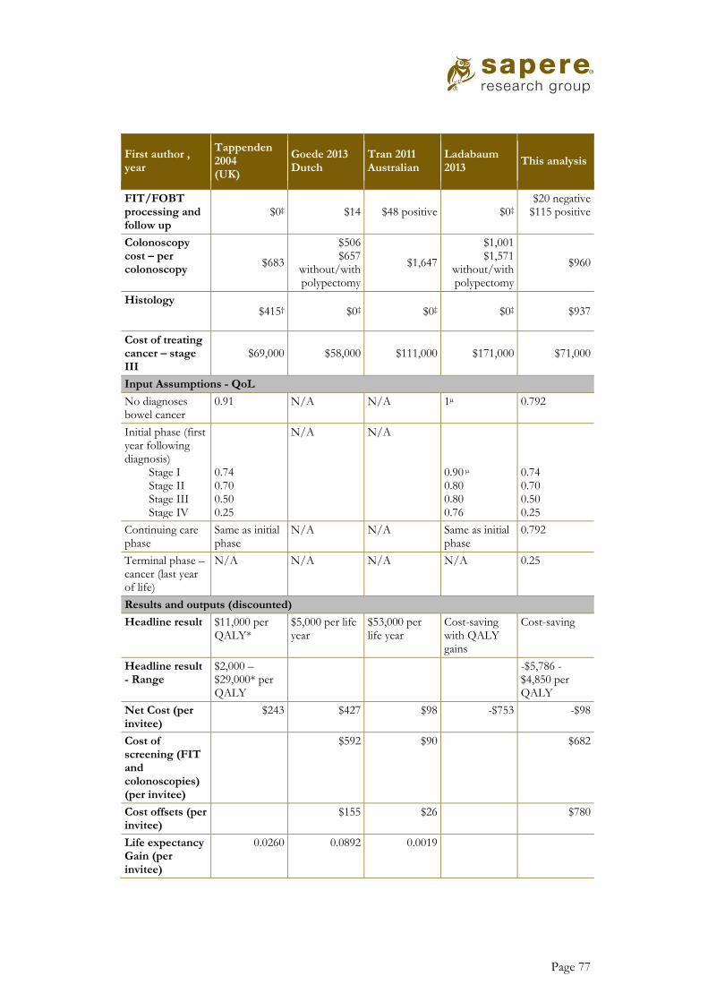
Page 77
First author , year
Tappenden 2004 (UK)
Goede 2013 Dutch
Tran 2011 Australian
Ladabaum 2013
This analysis
FIT/FOBT processing and follow up
$0‡ $14 $48 positive $0‡ $20 negative
$115 positive
Colonoscopy cost – per colonoscopy
$683
$506 $657
without/with polypectomy
$1,647
$1,001 $1,571
without/with polypectomy
$960
Histology $415† $0‡ $0‡ $0‡ $937
Cost of treating cancer – stage III
$69,000 $58,000 $111,000 $171,000 $71,000
Input Assumptions - QoL
No diagnoses bowel cancer
0.91 N/A N/A 1µ 0.792
Initial phase (first year following diagnosis)
Stage I Stage II Stage III Stage IV
0.74 0.70 0.50 0.25
N/A N/A 0.90 µ 0.80 0.80 0.76
0.74 0.70 0.50 0.25
Continuing care phase
Same as initial phase
N/A N/A Same as initial phase
0.792
Terminal phase – cancer (last year of life)
N/A N/A N/A N/A 0.25
Results and outputs (discounted)
Headline result $11,000 per QALY*
$5,000 per life year
$53,000 per life year
Cost-saving with QALY gains
Cost-saving
Headline result - Range
$2,000 – $29,000* per QALY
-$5,786 - $4,850 per QALY
Net Cost (per invitee)
$243 $427 $98 -$753 -$98
Cost of screening (FIT and colonoscopies) (per invitee)
$592 $90 $682
Cost offsets (per invitee)
$155 $26 $780
Life expectancy Gain (per invitee)
0.0260 0.0892 0.0019

Page 78
First author , year
Tappenden 2004 (UK)
Goede 2013 Dutch
Tran 2011 Australian
Ladabaum 2013
This analysis
QALY gain (per invitee)
0.0227 N/A 0.077 0.0730
Reduction in bowel cancer incidence
8.65% 10.39% δ 62% 35%
Reduction in bowel cancer mortality
23.42% 25.98% 75% 45%
*Tappenden et al 2004 included the following results in their report, Cost per QALY of £2,949.64 with a range of
£551 - £7,992. The marginal (net) cost was reported as £66.95. Costs reported in 2004 pounds
† Tappenden et al 2004 reported pathology costs of £30.00 and £250 for adenomas and cancers respectively.
When we calculated the average histology cost we applied a 62% weighting to adenoma based on the five year
volumes estimated by Tappenden.
‡ Assumed to be 0, as no values discussed or provided in the published reports.
Ω Ladabaum reported 40% of cancers in the base case, and 68% with FIT, would be diagnoses as localised. We
use these values to approximate the stage I cancers
µLadabuam reported the utility values used as 0.90, 0.80 and 0.76 for Localised, Regional and Distant cancer.
α Tran et al reported the participation rates for the ager groups 50, 55 and 65 as 28.0%, 37.7% and 46.4%
respectively
δ Tran et al reported that 1664 cases of bowel would be diagnosed with and without screening and that 225 cased
of bowel cancer would be avoided.
θ Tran et al state the sensitivity of FOBT as 66%. They reference Morikawa 200531 as the source, which reported
66% as the sensitivity for cancers, so we assume this value was only applied to cancers and not adenomas

Page 79
8. References
1 Sarfati D, Hill S, Blakely T et al. Is bowel cancer screening important for Maori? NZ Med J 13 August 2010, Vol 123 No 1320
2 Jackson C, Sharples K, Firth M et al. The PIPER Project: An Internal Examination of Colorectal Cancer Management in New Zealand, Health Research Council and Ministry of Health, 2015
3 New Zealand Guidelines Group. Guidance on surveillance for people at increased risk of
colorectal cancer 2011. Wellington: New Zealand Guidelines Group; 2011
4 Ministry of Health. Bowel Screening Pilot results. http://www.health.govt.nz/our-
work/diseases-and-conditions/cancer-programme/bowel-cancer-programme/bowel-screening-pilot/bowel-screening-pilot-results Accessed March 2016
5 Hol L, van Leerdam ME, van Ballegooijen M, van Vuuren AJ, van Dekken H, Reijerink JC,
van der Togt AC, Habbema JD, Kuipers EJ. Screening for colorectal cancer: randomised trial comparing guaiac-based and immunochemical faecal occult blood testing and flexible sigmoidoscopy. Gut. 2010 Jan;59(1):62-8. doi: 10.1136/gut.2009.177089. Epub .
6 Crotta S, Castiglione G, Grazzini G, Valle F, Mosconi S, Rosset R. Feasibility study of
colorectal cancer screening by immunochemical faecal occult blood testing: results in a northern Italian community. Eur J Gastroenterol Hepatol. 2004 Jan;16(1):33-7.
7 Grazzini G, Castiglione G, Ciabattoni C, Franceschini F, Giorgi D, Gozzi S, Mantellini P,
Lopane P, Perco M, Rubeca T, Salvadori P, Visioli CB, Zappa M. Colorectal cancer screening programme by faecal occult blood test in Tuscany: first round results. Eur J Cancer Prev. 2004 Feb;13(1):19-26
8 Fenocchi E, Martínez L, Tolve J, Montano D, Rondán M, Parra-Blanco A, Eishi Y.
Screening for colorectal cancer in Uruguay with an immunochemical faecal occult blood test. Eur J Cancer Prev. 2006 Oct;15(5):384-90.
9 Saito H. Colorectal cancer screening using immunochemical faecal occult blood testing in
Japan. J Med Screen. 2006;13 Suppl 1:S6-7.
10 Klabunde C, Blom J, Bulliard JL, Garcia M, Hagoel L, Mai V, Patnick J,Rozjabek H,
Senore C, Törnberg S. Participation rates for organized colorectalcancer screening programmes: an international comparison. J Med Screen. 2015 Sep;22(3):119-26. doi: 10.1177/0969141315584694. Epub 2015 May 12
11 Allison JE, Fraser CG, Halloran SP, Young GP. Population screening for colorectal cancer
means getting FIT: the past, present, and future of colorectal cancer screening using the

Page 80
fecal immunochemical test for hemoglobin (FIT). Gut Liver. 2014 Mar;8(2):117-30. doi: 10.5009/gnl.2014.8.2.117. Epub 2014 Mar 11. Review.
12 National Cancer Institute (USA), Colorectal Cancer Screening–for health professionals
(PDQ®) Evidence of Benefit. http://www.cancer.gov/types/colorectal/hp/colorectal-screening-pdq#section/_17 Accessed December 2015
13 European Commission. Segnan N, Patnick J, von Karsa L (eds), 2010. European
Guidelines for Quality Assurance in Colorectal Cancer Screening and Diagnosis - First Edition. ISBN 978-92-79-16435-4 .
14 Day LW, Bhuket T, Allison J. FIT testing: an overview. Curr Gastroenterol Rep. 2013
Nov;15(11):357. doi: 10.1007/s11894-013-0357-x. Review
15 Zheng S, Chen K, Liu X, Ma X, Yu H, Chen K, Yao K, Zhou L, Wang L, Qiu P, Deng Y,
Zhang S. Cluster randomization trial of sequence mass screening for colorectal cancer. Dis
Colon Rectum. 2003 Jan;46(1):51-8.
16 Nakajima M, Saito H, Soma Y, Sobue T, Tanaka M, Munakata A. Prevention of advanced
colorectal cancer by screening using the immunochemical faecal occult blood test: a case-control study. Br J Cancer. 2003 Jul 7;89(1):23-8.
17 Saito H, Soma Y, Koeda J, Wada T, Kawaguchi H, Sobue T, Aisawa T, Yoshida Y.
Reduction in risk of mortality from colorectal cancer by fecal occult blood screening with
immunochemical hemagglutination test. A case-control study. Int J Cancer. 1995 May
16;61(4):465-9
18 Saito H, Soma Y, Nakajima M, Koeda J, Kawaguchi H, Kakizaki R, Chiba R, Aisawa T,
Munakata A. A case-control study evaluating occult blood screening for colorectal cancer with hemoccult test and an immunochemical hemagglutination test. Oncol Rep. 2000 Jul-Aug;7(4):815-9
19 Heresbach D, Manfredi S, D'halluin PN, Bretagne JF, Branger B. Review in depth and
meta-analysis of controlled trials on colorectal cancer screening by faecal occult blood test.
Eur J Gastroenterol Hepatol. 2006 Apr;18(4):427-33. Review.
20 Hewitson P, Glasziou P, Watson E, Towler B, Irwig L. Cochrane systematic review of
colorectal cancer screening using the fecal occult blood test (hemoccult): an update. Am J Gastroenterol. 2008 Jun;103(6):1541-9. doi: 10.1111/j.1572-0241.2008.01875.x. Epub 2008 May 13. Review.

Page 81
21 Kronborg O, Jørgensen OD, Fenger C, Rasmussen M. Randomized study of biennial screening with a faecal occult blood test: results after nine screening rounds. Scand J Gastroenterol. 2004 Sep;39(9):846-51.
22 Lindholm E, Brevinge H, Haglind E. Survival benefit in a randomized clinical trial of
faecal occult blood screening for colorectal cancer. Br J Surg. 2008 Aug;95(8):1029-36. doi: 10.1002/bjs.6136.
23 Mandel JS, Bond JH, Church TR, Snover DC, Bradley GM, Schuman LM, Ederer F.
Reducing mortality from colorectal cancer by screening for fecal occult blood. Minnesota Colon Cancer Control Study. N Engl J Med. 1993 May 13;328(19):1365-71.Erratum in: N Engl J Med 1993 Aug 26;329(9):672.
24 Hardcastle JD, Chamberlain JO, Robinson MH, Moss SM, Amar SS, Balfour TW, James
PD, Mangham CM. Randomised controlled trial of faecal-occult-blood screening for colorectal cancer. Lancet. 1996 Nov 30;348(9040):1472-7
25 Center MM, Jemal A, Smith RA, Ward E. Worldwide variations in colorectal cancer. CA
Cancer J Clin. 2009 Nov-Dec;59(6):366-78. doi: 10.3322/caac.20038. Review.
26 Pharmaceutical Management Agency (PHARMAC). 2012. Prescription for
pharmacoeconomic analysis (PFPA). http://www.pharmac.health.nz/assets/pfpa-final.pdf.
Accessed May 2014.
27 Tran B, Keating CL, Ananda SS, Kosmider S, Jones I, Croxford M, Field KM, Carter RC, Gibbs P. Preliminary analysis of the cost-effectiveness of the National Bowel Cancer Screening Program: demonstrating the potential value of comprehensive real world data. Intern Med J. 2012 Jul;42(7):794-800. doi: 10.1111/j.1445-5994.2011.02585.x
28 Goede SL, van Roon AH, Reijerink JC, van Vuuren AJ, Lansdorp-Vogelaar I, Habbema
JD, Kuipers EJ, van Leerdam ME, van Ballegooijen M. Cost-effectiveness of one versus two sample faecal immunochemical testing for colorectal cancer screening. Gut. 2013 May;62(5):727-34. doi: 10.1136/gutjnl-2011-301917. Epub 2012 Apr 5.
29 Paul Tappenden, Simon Eggington, Richard Nixon, Jim Chilcott, Hannah Sakai, and Jon
Karnon. Colorectal cancer screening options appraisal Report to the English Bowel Cancer Screening Working Group. 2004
30 Ladabaum U, Allen J, Wandell M, Ramsey S. Colorectal cancer screening with blood-based
biomarkers: cost-effectiveness of methylated septin 9 DNA versus current strategies. Cancer Epidemiol Biomarkers Prev. 2013 Sep;22(9):1567-76. doi: 10.1158/1055-9965.EPI-13-0204. Epub 2013 Jun 24.
31 Morikawa T, Kato J, Yamaji Y, Wada R, Mitsushima T, Shiratori Y. A comparison of the
immunochemical fecal occult blood test and total colonoscopy in the asymptomatic population. Gastroenterology. 2005 Aug;129(2):422-8.
Page 82
32 Park DI, Ryu S, Kim YH, Lee SH, Lee CK, Eun CS, Han DS. Comparison of guaiac-
based and quantitative immunochemical fecal occult blood testing in a population at average risk undergoing colorectal cancer screening. Am J Gastroenterol. 2010 Sep;105(9):2017-25. doi: 10.1038/ajg.2010.179. Epub 2010 May 25
33 de Wijkerslooth TR, Stoop EM, Bossuyt PM, Meijer GA, van Ballegooijen M, van
Roon AH, Stegeman I, Kraaijenhagen RA, Fockens P, van Leerdam ME, Dekker E, Kuipers EJ. Immunochemical fecal occult blood testing is equally sensitive for proximal and distal advanced neoplasia. Am J Gastroenterol. 2012 Oct;107(10):1570-8. doi: 10.1038/ajg.2012.249.
34 Brenner H, Tao S. Superior diagnostic performance of faecal immunochemical tests for
haemoglobin in a head-to-head comparison with guaiac based faecal occult blood test among 2235 participants of screening colonoscopy. Eur J Cancer. 2013 Sep;49(14):3049-54. doi: 10.1016/j.ejca.2013.04.023. Epub 2013 May 22.
35 Morikawa T, Kato J, Yamaji Y, Wada R, Mitsushima T, Sakaguchi K, Shiratori Y.
Sensitivity of immunochemical fecal occult blood test to small colorectal adenomas. Am J Gastroenterol. 2007 Oct;102(10):2259-64.
36 Raginel T, Puvinel J, Ferrand O, Bouvier V, Levillain R, Ruiz A, Lantieri O, Launoy G,
Guittet L. A population-based comparison of immunochemical fecal occult blood tests for colorectal cancer screening. Gastroenterology. 2013 May;144(5):918-25. doi: 10.1053/j.gastro.2013.01.042. Epub 2013 Feb 1.
37 Faivre J, Dancourt V, Denis B, Dorval E, Piette C, Perrin P, Bidan JM, Jard C, Jung S,
Levillain R, Viguier J, Bretagne JF. Comparison between a guaiac and three
immunochemical faecal occult blood tests in screening for colorectal cancer. Eur J Cancer.
2012 Nov;48(16):2969-76. doi: 10.1016/j.ejca.2012.04.007. Epub 2012 May 7.
38 van Rijn JC, Reitsma JB, Stoker J, Bossuyt PM, van Deventer SJ, Dekker E. Polyp miss
rate determined by tandem colonoscopy: a systematic review. Am J Gastroenterol. 2006
Feb;101(2):343-50. Review.
39 Bressler B, Paszat LF, Chen Z, Rothwell DM, Vinden C, Rabeneck L. Rates of new or
missed colorectal cancers after colonoscopy and their risk factors: a population-based analysis. Gastroenterology. 2007 Jan;132(1):96-102
40 Szende A, Janssen B, Cabase´s J. Self-Reported Population Health: An International
Perspective based on EQ-5D. 2014. ISBN 978-94-007-7596-1 (eBook). DOI 10.1007/978-94-007-7596-1

Page 83
41 Ness RM, Holmes AM, Klein R, Dittus R. Utility valuations for outcome states
of colorectal cancer. Am J Gastroenterol. 1999 Jun;94(6):1650-7.
42 Ramsey SD, Andersen MR, Etzioni R, Moinpour C, Peacock S, Potosky A, Urban N.
Quality of life in survivors of colorectal carcinoma. Cancer. 2000 Mar
15;88(6):1294-303
43 Salomon JA, Haagsma JA, Davis A, de Noordhout CM, Polinder S, Havelaar AH, Cassini
A, Devleesschauwer B, Kretzschmar M, Speybroeck N, Murray CJ, Vos T. Disability weights for the Global Burden of Disease 2013 study. Lancet Glob Health. 2015 Nov;3(11):e712-23. doi: 10.1016/S2214-109X(15)00069-8
44 Färkkilä N, Sintonen H, Saarto T, Järvinen H, Hänninen J, Taari K, Roine RP. Health-
related quality of life in colorectal cancer. Colorectal Dis. 2013 May;15(5):e215-22. doi: .1111/codi.12143.
45 Downing A, Morris EJ, Richards M, Corner J, Wright P, Sebag-Montefiore D,
Finan P, Kind P, Wood C, Lawton S, Feltbower R, Wagland R, Vernon S, Thomas J, Glaser AW. Health-related quality of life after colorectal cancer in England: a patient-reported outcomes study of individuals 12 to 36 months after diagnosis. J Clin Oncol. 2015 Feb 20;33(6):616-24. doi: 10.1200/JCO.2014.56.6539. Epub 2015 Jan 5
46 Trentham-Dietz A, Remington PL, Moinpour CM, Hampton JM, Sapp AL, Newcomb
PA. Health-related quality of life in female long-term colorectal cancer survivors. Oncologist. 2003;8(4):342-9.
47 Arndt V, Merx H, Stegmaier C, Ziegler H, Brenner H. Quality of life in patients with
colorectal cancer 1 year after diagnosis compared with the general population: a population-based study. J Clin Oncol. 2004 Dec 1;22(23):4829-36. Erratum in: J Clin Oncol. 2005 Jan 1;23(1):248.
48 Blakely T, Atkinson J, Kvizhinadze G, Wilson N, Davies A, Clarke P. Patterns of cancer
care costs in a country with detailed individual data. Med Care. 2015 Apr;53(4):302-9. doi:
10.1097/MLR.0000000000000330. Erratum in: Med Care. 2015 Jun;53(6):560.
49 Ministry of Health. The Price of Cancer: The Public Price of Registered Cancer in New
Zealand. Wellington: Ministry of Health; 2011
50 Tilson L, Sharp L, Usher C, Walsh C, S W, O'Ceilleachair A, Stuart C, Mehigan B, John
Kennedy M, Tappenden P, Chilcott J, Staines A, Comber H, Barry M. Cost of care for colorectal cancer in Ireland: a health care payer perspective. Eur J Health Econ. 2012 Aug;13(4):511-24. doi: 10.1007/s10198-011-0325-z. Epub 2011 Jun 3.

Page 84
51 Lang K, Lines LM, Lee DW, Korn JR, Earle CC, Menzin J. Lifetime and treatment-phase
costs associated with colorectal cancer: evidence from SEER-Medicare data. Clin
Gastroenterol Hepatol. 2009 Feb;7(2):198-204. doi: 10.1016/j.cgh.2008.08.034. Epub 2008
Sep 4.
52 Ministry of Health 2015. WIESNZ14 cost weights. http://www.health.govt.nz/nz-health-
statistics/data-references/weighted-inlier-equivalent-separations/wiesnz14-cost-weights. Accessed May 2016
53 National Institute for Health and Care Excellence (NICE). Guide to the methods of
technology appraisal 2013. http://publications.nice.org.uk/pmg9
54 Ministry of Health. Provisional Mortality 2013 online tables. Published online 16
December 2015. http://www.health.govt.nz/publication/mortality-2013-online-tables
55 Rozen P, Liphshitz I, Barchana M. Follow-up of patients undergoing both semiquantitated
immunochemical fecal occult blood and colonoscopy examinations. Eur J Cancer Prev. 2012
May;21(3):247-53. doi: 10.1097/CEJ.0b013e32834c9cc6. PubMed PMID: 21955798
56 Pharmaceutical Management Agency (PHARMAC). Annual Report for the year ended 30
June 2015.
57 Pharmaceutical Management Agency (PHARMAC). Annual Report for the year ended 30
June 2012.
58 World Health Organisation. Threshold values for intervention cost-effectiveness by
Region. http://www.who.int/choice/costs/CER_levels/en/ Accessed March 2016
59 Statistics New Zealand 2016. Top statistics.
http://www.stats.govt.nz/browse_for_stats/snapshots-of-nz/top-statistics.aspx
Accessed March 2016
60 Lansdorp-Vogelaar I, Knudsen AB, Brenner H. Cost-effectiveness of colorectal cancer
screening. Epidemiol Rev. 2011;33:88-100. doi: 10.1093/epirev/mxr004. Epub 2011 Jun 1.
Reviewhttp://www.ncbi.nlm.nih.gov/pubmed/21633092
61 Carolyn M. RUTTER, Diana L. MIGLIORETTI, and James E. SAVARINO, Bayesian
Calibration of Microsimulation Models, Journal of the American Statistical Association,
December 2009, Vol. 104, No. 488, Applications and Case Studies, DOI:
10.1198/jasa.2009.ap07466
62 Muto, T., Bussey, H. J. R., and Morson, B. C. (1975), “The Evolution of Cancer in the
Colon and Rectum,” Cancer, 36, 2251–2270.
Leslie, A., Carey, F. A., Pratt, N. R., and Steele, R. J. C. (2002), “The Colorectal Adenoma–
Carcinoma Sequence,” British Journal of Surgery, 89, 845–860.
Page 85
63 Lee JK, Liles EG, Bent S, Levin TR, Corley DA. Accuracy of fecal immunochemical tests for colorectal cancer: systematic review and meta-analysis. Ann Intern Med. 2014 Feb 4;160(3):171. doi: 10.7326/M13-1484.
64 Rabeneck L, Rumble RB, Thompson F, Mills M, Oleschuk C, Whibley A, Messersmith H,
Lewis N. Fecal immunochemical tests compared with guaiac fecal occult blood tests for population-based colorectal cancer screening. Can J Gastroenterol. 2012 Mar;26(3):131-47
65 Hol L, Wilschut JA, van Ballegooijen M, van Vuuren AJ, van der Valk H, Reijerink JC, van
der Togt AC, Kuipers EJ, Habbema JD, van Leerdam ME. Screening for colorectal cancer: random comparison of guaiac and immunochemical faecal occult blood testing at different cut-off levels. Br J Cancer. 2009 Apr 7;100(7):1103-10. doi: 10.1038/sj.bjc.6604961