The Cost of Minimum Pension Guarantee

By

Tapen Sinha, ING Comercial America Chair Professor, Department of Actuarial Studies, Instituto Tecnológico Autónomo de México, Rio Hondo No. 1, Col. Tizapan-San Angel, 01000 Mexico, D.F., Mexico and Professor, School of Business, University of Nottingham, telephone: (52) 55-56-28-40-88, fax: (52) 55-56-28-40-86 (tapen@itam.mx, tapen.sinha@nottingham.ac.uk)

and Alejandro Renteria, Research Assistant, Department of Actuarial Studies, Instituto Tecnológico Autónomo de México, Rio Hondo No. 1, Col. Tizapan-San Angel, 01000 Mexico, D.F., México (arentes@gmail.com) Abstract: We model minimum pension guarantee using a simulation approach. Lachance and Mitchell (2002) have shown that it could be important if and when individual accounts are introduced in the United States. We model ours with real data from Mexico where individual accounts are already a reality and the minimum pension guarantee is already enshrined by law. We calculate the probability of the government needing to honor the guarantee and estimate the cost of such a promise using a real options approach. Higher investment in the stock market turns out to be the key. The higher the proportion of investment allowed by law in stocks, the lower the probability of government support.

Acknowledgement: We would like to thank the participants of the Actuarial Research Conference held in Mexico City in August 2005. We thank the Instituto Tecnológico Autónomo de México and the Asociación Mexicana de Cultura AC for their generous support of our research. Financial support for Alejandro Renteria was provided by the Sistema Nacional de Investigadores of the CONACYT for working as a research assistant to Tapen Sinha. However, we alone are responsible for the opinions expressed. They do not represent the views of the institutions with which we are affiliated.

Date: October 2005

Introduction

Governments often promise a minimum level of benefits under an accumulation

scheme. If future does not turn out to be rosy, what is the likelihood that the government

has to foot the bill of this guarantee? This question have been studied early on in the

Canadian context by Pesando (1982). It has been recently discussed in the US context by

Mitchell and Lachance (2002), Constantinides et al (2001) and Smetters (2001). Our

study examines the nature of this guarantee in Mexico. In Mexico, unlike the US, such

promises are already explicit in a system where individual accounts are a reality since

1997. Shah (2003) conducted another study in a developing country. Once again, the

study was done on a hypothetical basis as no pension privatization scheme exists in India.

Using the actual experience of the past eight years (1995-2005), and including actual

features of the Mexican system, we calculate the probability distribution of such

promises. In Mexico, the government has promised under the newly privatized publicly

mandated scheme, a minimum pension guarantee (MPG) for the workers who have been

in the labor force before July 1997. What effect does this guarantee have on the pension

system? What are the chances that an affiliate will actually have to be supported by the

government under the minimum pension guarantee scheme? Clearly, the results will

depend on the earnings of the individual over time and on the uncertainty of the rates of

return proportioned by their investments. In this paper, we calculate these probabilities.

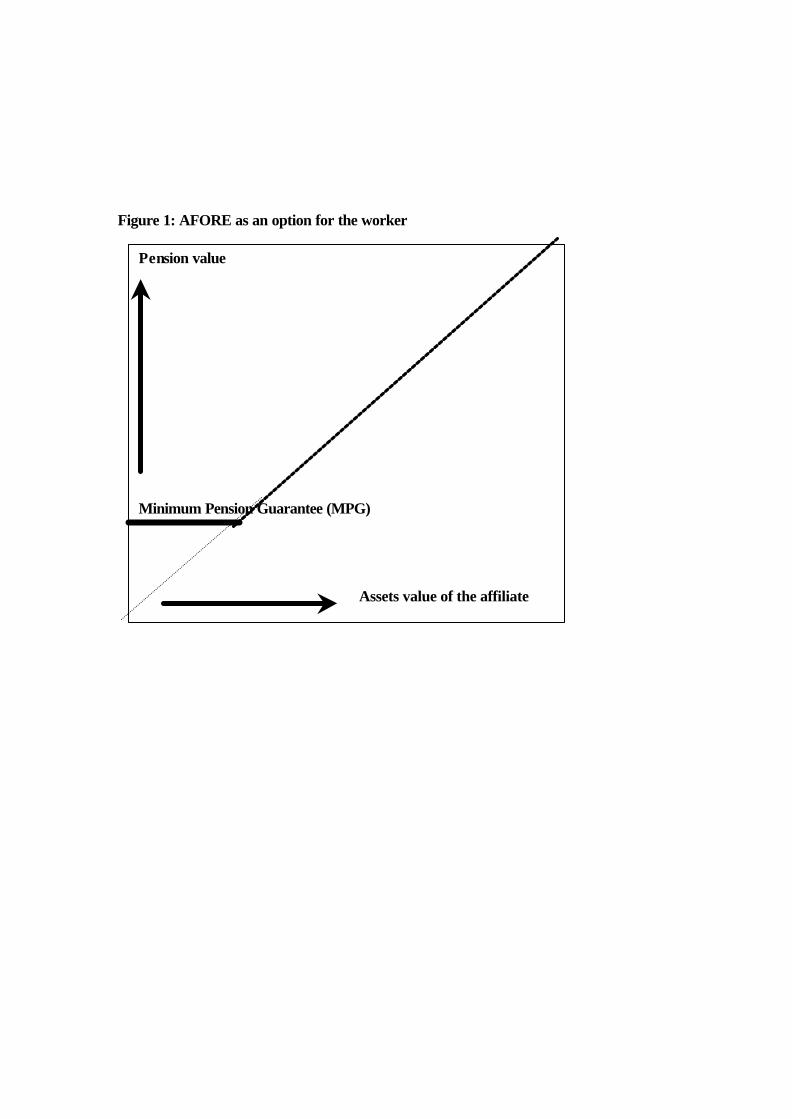
Figure 1: AFORE as an option for the worker

Pension value Minimum Pension Guarantee (MPG)

Assets value of the affiliate

Figure 1 shows that the MPG provides a floor for the pension benefits that a

worker can get if the funds accumulated falls short of one minimum salary (the MPG

promised by the government). Thus, it is like an option written by the government at no

cost to the worker because the guarantee is offered without cost. The option may be

exercised at retirement with an exercise price equal to the MPG. If the accumulated

assets in the individual account are less than the MPG, the option is in the money. The

worker will exercise the option. The government (and by implication, taxpayers) will

therefore assume the difference in value of the MPG and the assets in the fund.

Background on Pension Reform in Mexico

In 1997, Mexico moved from a defined benefits system (a la US Social Security)

to a defined contribution system (a la Chile). The system is publicly mandated but funds

are privately managed. The funds are called AFOREs (Administradoras de Fondos para

el Retiro). There are three components to each fund: government component, private

compulsory component and private voluntary component. There is a government

contribution. There is also a government guarantee that sets a floor value of one

minimum salary current as of July 1, 1997 indexed for inflation.

The minimum wage is an important concept in Mexico for wage setting. The

government from time to time resets the minimum wage. Many types of wage

negotiations are based on the value of the minimum wage. Minimum wage is not fixed in

real terms. It is fixed in nominal pesos. It is adjusted by legislation from time to time.

Therefore, it might be fixed in the short run but not necessarily in the long run. Over the

long run, the minimum wage has risen by less than the rate of inflation. Minimum wage

is set differently in different parts of the country. It is lower in rural areas. However,

when people talk about the minimum wage, they are usually talking about minimum

wage in Mexico City. In 1997, the minimum wage in Mexico City (lower in rural areas)

was about US$3.20 per day.

On July 1, 1997, the new privately administered but government mandated system

of retirement program came into existence in Mexico. This system has private companies

operating pension funds. Each company operating a pension fund is called an

Administradora de Fondos de Retiro or an AFORE. The investment fund, run by the

company is independent of the parent company, it is called a SIEFORE (Sociedad de

Inversion en Fondos de Retiro).

Each worker has an account with an AFORE. Funds are generated by

accumulation of contributions by the individual and by the yield generated by investment

by the AFORE. Thus, the contribution and the performance of the fund will solely

determine each person's pension benefit. The law also set a minimum pension guarantee.

There is a three way split, the employer pays 1.75%, the worker pays 0.625% and

the rest is paid by the government. This is called Seguros de Invalidez y Vida (IV). This

IV component is different from RCV under the new system. Under RCV, there is also a

three way split on contribution. The contribution of the employer is 5.15% of wages. The

employee contributes 1.125%. Thus, the total contribution of the employer and employee

is 6.225%. The government also will contribute an additional amount independent of the

wage of the person (more on that below). Table 1 below sets out the difference in the old

pay as you go scheme versus the new publicly mandated and privately funded pension

schemes.

Social Quota

The government contributes an additional amount independent of the wage of the

person. This additional contribution is called the Social Quota (cuota social). This

additional amount is 5.5% of the minimum in the Federal District of Mexico (also called

Mexico D.F., the municipality of Mexico City, excluding surrounding areas) as of July 1,

1997. Therefore, this amount is variable in the following sense. For a person earning an

equivalent of a minimum salary, this amounts to 5.5% of his or her salary along with the

other contribution of 6.5%. Hence, the total contribution amounts to 12% of the salary.

On the other hand, a person earning 10 times the minimum salary, the social contribution

is only 0.55% of wages. Thus, his or her total contribution will amount to 7.05% of

wages, a much smaller proportion. Of course in absolute amount this contribution will

be a much bigger number. There is a second important element of this social quota: this

segment of the contribution is exempt from charges imposed by an AFORE. Thus, this

portion accumulates without any fees.

Table 1: Contribution to Pensions in Mexico before and after Reform before reform after reform Contributions DOSL RDO LDA IMSS contribution 8.5% 4.5% 4.0% SAR sub-account 2.0% 2.0% INFONAVIT 5.0% 5.0% Cuota Social - 2.0% Total 13.5% 4.0% Contributors 15.50% 17.50% Employer 12.95% 12.95% Employee 2.125% 2.125% Government 0.425% 2.425%

Notes: Cuota social is government contribution under the new regime. It is not exactly 2.0%, it is set at 5.5% of minimum wage. Hence it varies with the wage rate. In 1997, the contributed amount was 2.0% for average worker. DOSL = Disability, Old age, Severance at Old age, and Life insurance. It was also called IVCM. RDO = Retirement, severance at Old age, and Old age. LDA = Life and disability assurance.

Changes in Investment Regime

The investment portfolio of the privatized government mandated pension funds

permitted by law in Mexico used to be extremely limited. CONSAR had set out the

general rules of investment under various circulars. These rules as they applied in 1997

are listed in Table 2.

Table 2: Pension Fund Investment Guidelines circa 1997 Types of Assets % of asset value I Inflation Linked Bonds 51% minimum IIa Bonds issued by either the Federal Government or Banco de Mexico 100% max IIb Bonds issued by either the Federal Government or Banco de Mexico in US dollars

10% max

IIc Corporate bonds, Bank issued bonds, Financial intermediary bonds 35% max IId Bonds issued by banks and other financial intermediaries 10% max IIe Repurchase Agreements 5% max IIf Checking accounts $250,000 max IIIa Bonds issued by a single issuer (except Federal Government or Banco de Mexico)

10% max

IIIb Bonds issued by a company where fund manager has interest 5% max IIIc Bonds issued by companies as parts of single holding company 15% max IIId % of a single issue (except Federal or Banco de Mexico) 10% max IV Bonds with maturity less than 183 days 65% min

Several features of the investment regime are worth noting. First, all investments

have to be in the form of bonds and nothing else. Second, there is a requirement of a

minimum of 51% investment to be made in inflation linked bonds. Third, at least 65% of

all the bonds held have to have a maturity of 163 days or less. For a newly founded

system, the first two restrictions made sense. Mexico has suffered high volatility in the

stock market. Thus, allowing for investment in stocks right off the bat may not be a good

idea to earn credibility of the affiliates. The second restriction also makes sense for a

country that has suffered over 50% inflation rate as recently as 1995. However, having all

pension funds investing the vast majority of their funds in short term bonds (less than 6

months of maturity) makes much less sense. At the time, the funds held their portfolios

with bond maturity of less than 100 days. For funds that will pay in twenty to thirty years,

this is a severe and unnecessary restriction.

For private sector investment, the theoretical limit was 35%. But, for private

bonds, it not only specifies the amount, but also the quality of investment. For example,

the minimum bond rating (by Standard and Poors) should be at the minimum mxA-3 for

the short run and mxAA for the long run. In practice, very limited number of companies

could comply with such highly rated bonds and hence, the AFOREs held very little of the

private bonds.

The investment regime has been relaxed in 2005. Each AFORE is allowed to have

two separate portfolios. The first portfolio is more conservative than the second one. The

second one is allowed to invest in not just bonds but as well as stocks as long as there is

capital guarantee. Not all workers are eligible to choose Fund 2. Only workers of age 55

or below can choose Fund 2.

Table 3: Investment Regimes of AFOREs in 2005

SIEFORE Fund 1 SIEFORE Fund 2 Type Upper

Limit Upper Limit

Government bonds v 100% v 100% Private debt with ratings mxA-1+ and mxAAA1 v 100% v 100%

Private debt with ratings mxA-1 and mxAA1 v 35% v 35%

Private debt with ratings mxA-2 and mxA1 v 5% v 5%

Value of foreign debt v 20%

Foreign debt v 20% Structured notes with capital protection v 15%

With this relaxation of requirements, it is still difficult for the funds to invest in

stocks. The structured notes with capital protection only allow the AFOREs to construct

synthetic options for stock market participation. Direct participation in stocks is still not

possible. In the future, participation in the stock market might become possible. In the

following section, we examine how the portfolios of the AFOREs have behaved over the

past eight years.

1 Private debt with ratings by Standard & Poor’s

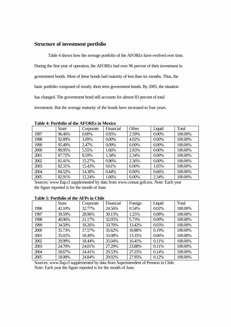
Structure of investment portfolio

Table 4 shows how the average portfolio of the AFOREs have evolved over time.

During the first year of operation, the AFOREs had over 96 percent of their investment in

government bonds. Most of these bonds had maturity of less than six months. Thus, the

basic portfolio composed of mostly short term government bonds. By 2005, the situation

has changed. The government bond still accounts for almost 83 percent of total

investment. But the average maturity of the bonds have increased to four years.

Table 4: Portfolio of the AFOREs in Mexico State Corporate Financial Other Liquid Total 1997 96.46% 0.00% 0.95% 2.59% 0.00% 100.00% 1998 92.89% 3.09% 0.00% 4.02% 0.00% 100.00% 1999 95.49% 2.47% 0.09% 0.00% 0.00% 100.00% 2000 89.95% 5.55% 1.66% 2.83% 0.00% 100.00% 2001 87.72% 8.59% 1.34% 2.34% 0.00% 100.00% 2002 81.41% 15.27% 0.96% 2.36% 0.00% 100.00% 2003 82.31% 15.43% 0.61% 0.00% 1.65% 100.00% 2004 84.52% 14.38% 0.44% 0.00% 0.66% 100.00% 2005 82.91% 12.24% 1.66% 0.00% 2.34% 100.00% Sources: www.fiap.cl supplemented by data from www.consar.gob.mx. Note: Each year the figure reported is for the month of June. Table 5: Portfolio of the AFPs in Chile State Corporate Financial Foreign Liquid Total 1996 42.10% 32.77% 24.56% 0.54% 0.02% 100.00% 1997 39.59% 28.96% 30.13% 1.25% 0.08% 100.00% 1998 40.96% 21.17% 32.05% 5.73% 0.09% 100.00% 1999 34.59% 18.26% 33.70% 13.42% 0.03% 100.00% 2000 35.73% 17.57% 35.62% 10.88% 0.19% 100.00% 2001 35.02% 18.49% 33.08% 13.35% 0.06% 100.00% 2002 29.99% 18.44% 35.04% 16.41% 0.11% 100.00% 2003 24.70% 24.01% 27.29% 23.88% 0.11% 100.00% 2004 18.67% 24.41% 29.53% 27.25% 0.14% 100.00% 2005 18.08% 24.84% 29.02% 27.95% 0.12% 100.00% Sources: www.fiap.cl supplemented by data from Superintendent of Pension in Chile. Note: Each year the figure reported is for the month of June.

To contrast the situation in Mexico, we compare the average portfolio of the AFPs

in Chile. Table 5 shows that the investment in the government sector has dramatically

fallen from 42 percent to 18 percent. Interestingly, foreign investment has taken up the

entire shift in the portfolio. With liberalization of investment, we might see similar

changes in the portfolio compositions in Mexico.

Who is eligible for the minimum pension

The Federal Government offers MPG free of charge. It offers a life annuity of the

equivalent of one minimum salary to be paid monthly indexed to the inflation (as

measured by the consumer price index in Mexico called INPC). The payment will be

made to all workers who satisfy the following requirements2: (1) Contribute at least 1250

weeks, 24 years, in the system. The payments do not have to be continuous. Under the

old pay as you go system, to qualify for the old age pension, a person has to have a

minimum contribution of 500 weeks and aged 65 years (60 years for people classified as

"too old to work"). For people to be eligible to collect disability pension, at least 150

weeks of contribution is required. In addition, it requires a certification from IMSS about

the disability. However, the contribution had to be continuous. Therefore, a person

contributing one month less than the required number of months would lose the right for

a pension entirely. (2) The person has 65 years of age. (3) The amount of resources

accumulated at the point of retirement is insufficient for buying a life annuity equivalent

of the minimum pension guarantee.3 Thus, the cost of financing such a minimum pension

2 Ley del Seguro Social, Article 170. 3 Ley del Seguro Social, Article 171.

guarantee is a liability for the government. Our paper is an attempt to value such a

liability.

How many are getting minimum pension?

The number of people who are getting minimum pension is rising over time. The

total number of people receiving minimum pension under the new regime is given in the

following Figure x. Since the system is in its infancy, the number of people receiving it is

very small. As the system matures, over the next three decades, the number will rise

reaching several millions.

Figure 2: Number of minimum pension recipients 1997-2005 (August)

196

9301,316

1,7622,218

2,835

3,505

4,0844319

0

1000

2000

3000

4000

5000

1997 1998 1999 2000 2001 2002 2003 2004 2005

Modeling the Cost of Minimum Pension Guarantee

Investment

We assume that a fraction ? (lambda) of the accumulated resources of the

individual account will be invested in stocks and the rest (1-?) will be invested in bonds.

We assume that the bonds are risk free and the entire risk comes from stock portfolio. We

will also assume that this fraction lambda will stay constant throughout the investment

period. We assume that the stock portfolio has a Normal distribution with mean µM and

standard deviation σM. We explain this assumption in our context further below.

Commissions

In our calculations, we use the commissions charged in April 2005. Commissions

are a moving target. Over time, the structure of commissions have changed. For example,

one company used to charge on real rate of return. The company now charges on the flow

of funds. A number of companies have merged with others. Their commission structures

have changed after the mergers. Some new companies have started operating. However,

for all our calculations, we do take into account the discounts offered by the AFOREs.

Many AFOREs allow a reduction in commission for every year a person stays with that

AFORE.

Contributions

We consider two separate sets of contributions. (1) The contribution of 6.5

percent of the base salary for each worker. (2) The contribution of 5.5 percent of

minimum salary contributed by the government. It is necessary to treat these two sets

separately as the contribution from the base salary attracts commissions of the AFOREs

but by law, the government contribution does not. (3) We calculate everything on the

basis of a monthly contribution. There is a third component of 5 percent of the base

salary that goes into a separate housing account. It is not part of the retirement account. In

our calculation, the housing account is not taken into account.

Inflation

Since 1998, inflation in Mexico has come down to a single digit. The central bank

has become independent. We can reasonble suppose that the monetary policy in the

future will ensure that inflation stays under control. All our calculations are calculated in

real terms using the pesos of April, 2005. There are two elements in the calculations that

are related to inflation adjustment: minimum salary and social quota. We are going to

assume that both of them are adjusted for inflation one for one.

Salary

We assume an initial salary of W which has a constant annual increment of ?W.

For the change of salary over time, we consider two scenarios for the value of ?W.

Constant salary over time. There is no real increase in salary. In other words,

? W=0 for all periods.

There is a constant increase in salary over the years in real terms: ?W=2.5

percent. This increase does not change over time.

It should be noted that for workers with earnings between the equivalent of one minimum

salary and three minimum salaries, the salary increase in real terms has been close to zero

in the decade of 1996-2005. In the subsequent discussion, all salaries are expressed in

multiples of minimum salary current in April of 2005. The value of the minimum salary

in April 2005 was $45.24 pesos daily. However, the social quota and the minimum

pension guarantee are by law set for July 1997. Therefore, for all our calculations, the

minimum wage used for calculating the social quota and minimum pension guarantee are

set at $53.6 pesos daily adjusting for inflation during July 1997 and March 2005.

Figure 3: Salary structure of workers in Mexico covered by the system 2004

Figure 3 above shows the salary structure of workers covered in the formal

system. More than half the workers earn below the equivalent of 3 times the minimum

salary. What we shall show is that for workers earning 3 times the minimum salary or

less are most likely to claim minimum salary benefits. Therefore, the majority of the

workers are likely to make that claim.

Periods of contributions

For this paper, we assume two sets of periods of contributions: 40 years and 25

years with a retirement age of 65. The first period is based on the idea that a worker is

likely to work full time between age 25 and 65 therefore working full time over a period

of 40 years. The second period of contribution of 25 years is the minimum required for

being eligible for a minimum pension. Although it is unlikely that full time male workers

1 to 3 MW

4 to 5 MW

6 to 10 MW

More than 10 MW

Source: IMSS

55.68%

20.65%

15.06%8.6%

Salary level of workers under the IMSS system2004

will be in the labor force for 25 years only, the calculation is important for the following

reason. About half of the people in the labor force in Mexico work in the informal sector.

So, it is easy for workers to complete 25 years of work in the formal labor force, acquire

the right to minimum pension and then work in the informal sector. In the past, we have

seen such situations in a high number of cases (where, under the old system, the workers

acquired the right to a pension only after ten years of work). In both calculations, we

assume the total number of years of contribution is contiguous.

We use the following accumulation process to generate our scenarios:

ttftr

t CVrVV Mte ++−+=+ )1)(1(1 λλ

where t refers to a period with t = 0,1,2,..., T.

Vt Wealth accumulated at time t for the individual account.

? Percentage of wealth invested in stocks at every period t.

rMt (Variable) real rate of return of stocks at time t.

rf Fixed real interest rate earned by government bonds.

Ct Worker contribution at time t

The contribution at time t Ct has three separate elements that varies with time t.

csBSComC ttt +−= )065(.

Ct Net contribution of the worker at time t.

Comt Commission charged by the AFORE at time t. This amount varies with time

because the discount the AFOREs offer.

BSt Base salary at time t.

cs Social quota.

To keep the number of scenarios manageable, we take the AFOREs which charge

the most and the AFOREs which charge the least amount of commissions as well as the

average commission of all the AFOREs as of April 2005.

We use the above equations to work out 1,000 trajectories for each salary level for

different values of lambda for T = 480 and T = 300 months (recall that our analysis is

done using monthly data – 480 months correspond to 40 years and 300 months

correspond to 25 years).

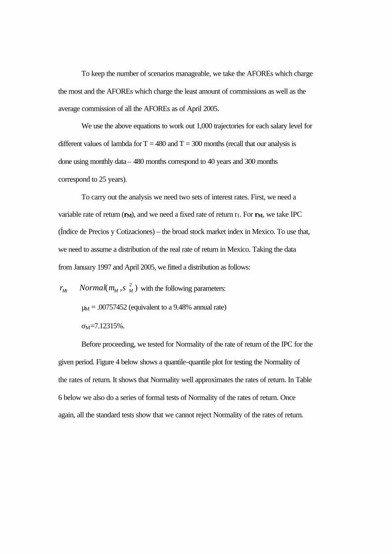
To carry out the analysis we need two sets of interest rates. First, we need a

variable rate of return (rM), and we need a fixed rate of return rf. For rM, we take IPC

(Índice de Precios y Cotizaciones) – the broad stock market index in Mexico. To use that,

we need to assume a distribution of the real rate of return in Mexico. Taking the data

from January 1997 and April 2005, we fitted a distribution as follows:

),( 2MMMt Normalr σµ∝ with the following parameters:

µM = .00757452 (equivalent to a 9.48% annual rate)

σM=7.12315%.

Before proceeding, we tested for Normality of the rate of return of the IPC for the

given period. Figure 4 below shows a quantile-quantile plot for testing the Normality of

the rates of return. It shows that Normality well approximates the rates of return. In Table

6 below we also do a series of formal tests of Normality of the rates of return. Once

again, all the standard tests show that we cannot reject Normality of the rates of return.

Figure 4: Quantile-quantile plot for the rates of return of IPC 1997-2005

-3

-2

-1

0

1

2

3

-.20 -.15 -.10 -.05 .00 .05 .10 .15 .20

IPC

Nor

mal

Qua

ntile

Theoretical Quantile-Quantile

Table 6: Testing for Normality of the rates of return

Hypothesis: Normal Included observations: 110 Method Value Adj. Value Probability Lilliefors 0.071154 > 0.1 Cramer-von Mises 0.086099 0.086490 0.1708 Watson 0.078976 0.079335 0.1809 Anderson-Darling 0.486738 0.490147 0.2207

For each period, we assume one realization of this distribution. For risk free

interest rate (rf), we took the real monthly interest rate of BONDES 182 – the Federal

Government bond that pays interest every three months with an inflation protection.

Recall from Tables 2 and 3 that such bonds form a great part of AFORE portfolios. These

government bonds will continue to be the major part of portfolios of the AFOREs well

into the next decades. The interest rate was 4.63 percent annual real over the period

January 1997 and April 2005.

In summary, the assumptions of our model are:

- Valuation date of April 2005

- Continuous contribution of 25 or 40 years

- Retirement age: 65 years

- Payment made monthly

- Inflation: 0 percent – all figures calculated in real terms

- Base salary (BS) . BS = 1, 10, 15, 20 and 25 SM4

- Salario Mínimo (SM). $45.24 pesos daily

- Salario Mínimo of 1997 adjusted for inflation (SM97) to $53.60 pesos daily

- Salary rise (?W). 0% y 2.5% annual

- Commissions (Comt). Current structure of four AFOREs with charges current

at that date taking into account the discount that every AFORE offers.

- Contribution (Ct). 6.5% of base salary minus the commissions charged plus

the social quota (that is free of commissions)

- Social quota $2.94 pesos per day.

- Risk free interest rate (rf). 4.63% annual

- Variable market rate (rM) is Normal with mean µM = 9.48% annual and

standard deviation σM = 7.12%

- Investment percentage in stocks. λ = 0% to 100% with 5% steps.

4 Salário Mínimo is the minimum salary current as of April 2005

Formulas for calculating the single premium and the probability

The guarantee offered by the government is 53.60 pesos in April 2005. In

addition, the guarantee also contains a clause of the paying 90% of the benefits to the

surviving spouse. So, we have to take into account a joint pension authorized by the

government. According to the data from the INEGI, the Mexican Census Bureau, the

majority of men of the relevant age are married and in more than 80 percent of the cases,

the men are between three to five years older than their wives. de los matrimonios el

hombre es mayor de 3 a 5 años. 5 For calculating the single premium for the annuity in

question, we used the following mortality tables: EMSSAH-97 for men and EMSSAM-

97 for women. These are the tables recommended by the CNSF.6

For calculating the net premium for the single payment annuity, we use the

following formula:

)1())1.9(.( )12()12(97 smfääSMPN xyx ++•+•=

where

PN Net premium for the annuity

SM97 Minimum salary of 1997 indexed for inflation

x Age at retirement: 65 years

y Age of the wife of the worker, 61 years (the average difference in Mexico

between workers and their wives is four years)

f Administrative and acquisition fee of 1% (see footnote 6)

sm Security margin 2% (see footnote 6)

5 Data from INEGI, 2000 6 Circular S22.3.4 of the CNSF

The interest rate for calculating the annuity is taken to be 3.5 percent as

recommended by the CNSF (see footnote 6). The amount of the single premium required

to pay the MPG is calculated at 321,410.00 pesos in April 2005.

Finally, we calculate the probability of exercising the option with the following:

N

SFPROB PNSFi

BSi

BSBSi

∑<∃= ,

,

where,

PROBBS Probability of exercising the MPG option for the workers whose base

salary is BS

BS Base salary

SFi,BS Final accumulated sum for indvidual i with initial salary BS

PN Net premium cost for the MPG

N Number of times the experiment is conducted.

Conceptually, we can think of the pension guarantee as an implicit European put

option for the government. At the moment of retirement (maturity date of the option), the

worker an option offered by the government. If the accumulated value of the worker in

his account falls below what is needed to buy the MPG (calculated at 321,410.00 pesos),

the worker is going to exercise the option.

The following figure explains the option.

Figure 5: The Implicit Put Option

Payoff at T denoted by P(T) is valued as follows

}0,max{)( TVPNTP −=

where,

P(T) Price of the option at the moment of retirement T.

PN Strike Price, net premium of the life annuity equivalent of the MPG.

VT Value of the underlying asset – the value of the asset in the individual

account at time T.

Payoff (T) = max{ MPG – VT , 0}

MPGVT

Pay

off

For calculating the value of the option, we use the standard Black and Scholes

(1973) option valuation model. This model holds only under the existence of complete

markets. It is difficult to imagine complete markets in the current context, but we can still

use this pricing to be used as a benchmark.

Results The results are demonstrated in Appendices A, B, and C. Case 1: The worker is in

the system for 40 years. The first striking feature is that for individuals earning the

equivalent of one minimum salary, the probability of not receiving the minimum pension

is 1 if low amounts are invested in the high risk/high return asset. This probability

diminishes with rising investment in the stock market. The second striking feature is that

with rising levels of income, this probability falls rapidly. Case 2: The worker is in the

system for 25 years. Once again, the probability of not getting minimum pension is very

high for low income persons even when the investment in the high risk/high return asset

is high. This probability does not diminish rapidly for rising levels of income.

In the final part, we show the value of the option using standard Black-Scholes

valuation model. Once again, the behavior of the option value has the same structure as

the probability of not getting the minimum pension.

Conclusions

Our results show that in many circumstances, the low income individuals are

likely to fall back on the minimum pension. It is the low income people who are likely to

have sporadic payments into the system over time. Thus, they are also more likely to

become eligible by making the minimum number of contributions. It is well known that

many employers pay lower salary “over the table” and compensate the workers by paying

extra “under the table.” It is beneficial for workers as they do not have to pay taxes on

such undeclared income. If this practice is that widespread, it is quite possible that we

shall see more than half of the workers end up falling back on the minimum pension

benefits in the formal sector. It appears from all the scenarios that investment in the stock

market appears to be unambiguously a good thing.

References

Black, Fischer & Scholes, Myron (1973), "The pricing of options and corporate

liabilities," Journal of Political Economy 81, 637–654.

Constantinides, George M., Donaldson, John B. and Mehra, Rajnish (2002),

"Junior must pay: Pricing the implicit put in privatizing social security," NBER Working

Paper No. 8906.

Lachance, Eve-Marie and Olivia Mitchell. (2002), Understanding individual

account guarantees, NBER Working Paper No. 9195.

Pesando, James, (1982), “Investment Risk, Bankruptcy Risk, and Pension Reform

in Canada.” Journal of Finance, 741 - 49.

Shah, Ajay, (2003), "Investment risk in the Indian pension sector and the role for

pension guarantees," Working Paper, Department of Finance, New Delhi, India.

Smetters, Kent (2000), The design and cost of pension guarantees, The Wharton

School, University of Pennsylvania.

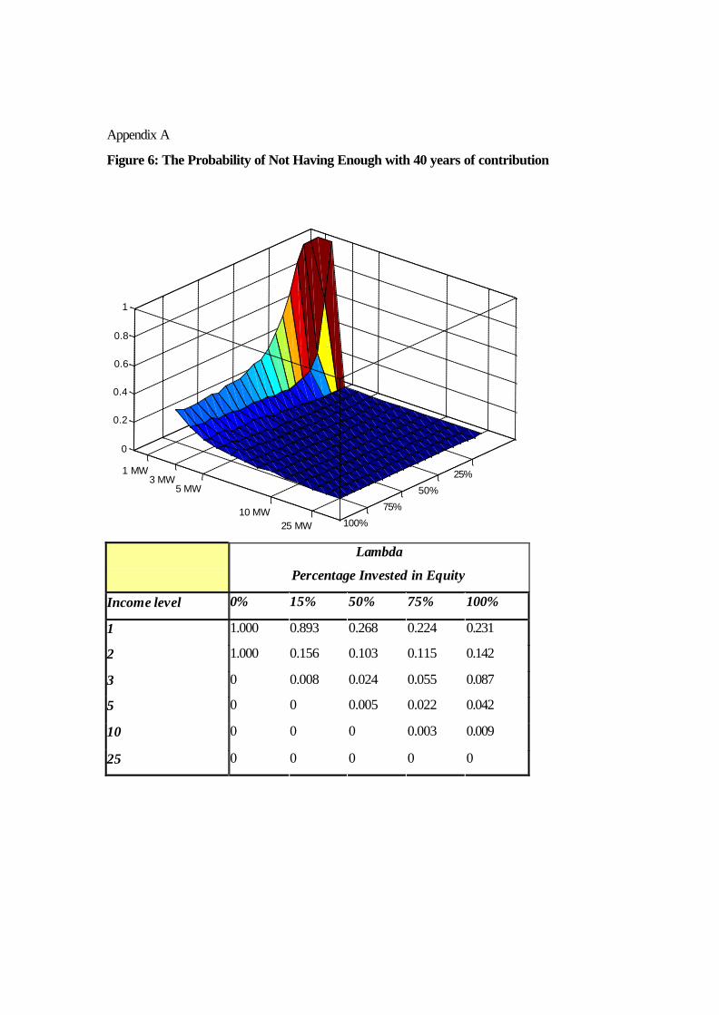
Appendix A

Figure 6: The Probability of Not Having Enough with 40 years of contribution

Lambda

Percentage Invested in Equity

Income level 0% 15% 50% 75% 100%

1 1.000 0.893 0.268 0.224 0.231

2 1.000 0.156 0.103 0.115 0.142

3 0 0.008 0.024 0.055 0.087

5 0 0 0.005 0.022 0.042

10 0 0 0 0.003 0.009

25 0 0 0 0 0

50%

100%

25%

75%

5 MW3 MW

10 MW 25 MW

1 MW

0

0.2

0.4

0.6

0.8

1

Appendix B

Figure 7: The Probability of Not Having Enough with 25 years of contribution

0.0060.00100025 0.0990.0580.0340010 0.2970.2840.3270.8931.0005 0.4430.4990.6941.0001.0003 0.6030.6800.8631.0001.0002 0.7280.8290.9671.0001.0001

100%75%50%25%0%Income

Lambda Percentage Invested in Equity

0

50%

100%

25%

75%

5 MW3 MW

10 MW 25 MW

1 MW

0

0.2

0.4

0.6

0.8

1

Appendix C

Figure 8: Option value for each level of income and investment composition

.256.073 000 25 73 100 10

3224 214278 5 5450 63119147 3 8185 103161181 2

116127 158201216 1

100%75% 50%25%0% Income

Lambda Percentage Invested in Equity

15%

50%75%

100%

5 MW

10 MW

1 MW3 MW

25 MW

50,000

100,000

150,000

200,000

250,000