The Costs and Benefits of Financial Advice∗

Stephen Foerster Juhani Linnainmaa Brian Melzer Alessandro Previtero

March 8, 2014

Please do not cite or quote without authors’ permission

Abstract

We assess the value that financial advisors provide to clients using a unique panel dataset on

the Canadian financial advisory industry. We find that advisors influence investors’ trading

choices, but they do not add value through their investment recommendations when judged

relative to passive investment benchmarks. The value-weighted client portfolio lags passive

benchmarks by more than 2.5% per year net of fees, and even the best performing advisors fail

to produce returns that reliably cover their fees. We show that differences in clients’ financial

knowledge cannot account for the cross-sectional variation in fees, which implies that lack of

financial sophistication is not the driving force behind the high fees. Advisors do, however,

influence client savings behavior, risky asset holdings, and trading activity, which suggests that

benefits related to financial planning may account for investors’ willingness to accept high fees

on investment advice.

∗Stephen Foerster is with the Western University, Juhani Linnainmaa is with the University of Chicago BoothSchool of Business and NBER, Brian Melzer is with the Northwestern University, and Alessandro Previtero is with theWestern University. Shlomo Benartzi, Antonio Bernardo, Chuck Grace, Luigi Guiso, Antoinette Schoar (discussant),Barry Scholnick, and Dick Thaler for valuable comments. We are also grateful for feedback given by seminar andconference participants at Nanyang Technological University, Singapore Management University, National Universityof Singapore, Rice University, Yale University, University of Washington, SUNY-Buffalo, Federal Reserve Bank ofCleveland, University of Chicago, American Economic Association 2014 meetings, and University of Alberta. We areespecially grateful to the Household Finance Advisory Council members for donating data and giving generously oftheir time by helping us to better understand the complexity of the mutual fund industry. Zhou Chen and BrianHeld provided helpful research assistance. Address correspondence to Alessandro Previtero, Western University, 1255Western Road, London, Ontario N6G 0N1, Canada (email: aprevitero@ivey.ca).

1 Introduction

Individual investors rely extensively on financial advisors to guide their investment and savings

decisions. For example, in the United States roughly 40% of households that own mutual funds

made purchases through an independent financial planner, and a similar proportion made purchases

through a full-service investment broker (Investment Company Institute 2013). Likewise, among

Canadian retail investors roughly 60% of assets are in accounts directed by financial advisors,

while full-service brokers manage another 20% of assets (Canadian Securities Administrators 2012).

Despite investors’ widespread use of financial advisors, relatively little is known about the cost of

advisors’ services and the quality of their advice. This paper helps to fill that void by measuring the

costs of financial advice for a large sample of advisory clients, and assessing the benefits reflected

in those clients’ investment and savings choices.

It remains an open question whether and to what extent financial advisors add value. Given

the complexity of asset allocation, investment selection and optimal savings decisions, as well as

the potential for self-directed investors to make mistakes due to lack of financial knowledge or

behavioral biases, there is substantial scope for advisors to add value.1 On the other hand, pricing

for advisory services is often opaque and advisor quality is difficult to assess, which can dull the

market forces that would otherwise reduce prices or improve quality. Indeed, there is evidence that

competition is ineffective in reducing price mark-ups within retail asset management (Hastings,

Hortacsu, and Syverson 2013). Furthermore, the typical compensation scheme—whereby advisors

1There is a large literature documenting the behavioral biases of individual investors. Barber and Odean (2000,2001, 2002) show that investors lose by trading too much, and link this tendency to overconfidence in one’s owntrading abilities. Grinblatt and Keloharju (2000, 2001) show that individual investors perform worse than institutionalinvestors, and that investors exhibit a “disposition effect,” a preference to sell stocks with unrealized capital gainsrather than those with capital losses. Benartzi and Thaler (2001), Choi, Laibson, and Madrian (2005), and Calvet,Campbell, and Sodini (2007) show that individual investors under-diversify.

1

are paid through commissions on the investment products they sell—creates an agency conflict,

which can harm naıve investors and limit value added even in a market populated by well-informed

investors.2 These supply-side considerations offer reasons why the value of financial advice may be

limited.

To provide further evidence on the value of financial advice, we take advantage of uniquely

detailed and extensive data furnished by three large financial institutions. The data include

transaction-level records on over ten thousand financial advisors and these advisors’ one million

Canadian clients, along with demographic information on both investors and advisors. Importantly,

the data cover a substantial portion—roughly 10%—of the non-bank advisory industry in Canada,

which allows us to overcome a limitation of other research on this topic, which studies smaller and

potentially unrepresentative groups of investors and advisors. The data also include useful individ-

ual characteristics such as age and financial knowledge, which allows us to explore differences in

the costs and benefits of advice in the cross-section of households.

Our analysis proceeds as follows. First, we quantify the costs of advice and characterize the

distribution of fees across investors and advisors. The investors in our sample pay an average

expense ratio equal to 2.43% (1.8% at the 10th percentile versus 2.8% at the 90th percentile).

The average investor pays $1,575 per year for financial advice, but this amount varies considerably

across investors because fees are proportional to assets under management. While investors in the

bottom decile pay as little as $55 per year, those in the top decile pay more than $3,918 per year.

Next, we assess the quality of advisors’ investment advice. We begin by evaluating the invest-

ment performance of advised clients. Net of fees, we find evidence of substantial underperformance

2In theoretical work, Inderst and Ottaviani (2009) examine the effects of such agency conflicts on householdwelfare. In empirical work on this topic, Hackethal, Inderst, and Meyer (2012) find that investors who rely moreheavily on advice have a higher volume of security transactions and are more likely to invest in products that salesmenare incentivized to sell.

2

relative to passive investment benchmarks. In aggregate, advised portfolios lag passive benchmarks

by 2% to 3% per year, depending on the choice of benchmark. These estimates represent economi-

cally substantial underperformance: an investor who expects to retire in 30 years gives up a quarter

of potential savings in present value terms by lagging the passive benchmarks by 3% per year.

It is the performance drag from fees and not negative stock-picking or market-timing abilities

that accounts for most of this underperformance. The value-weighted expense ratio of the average

advisor in the sample is 2.4% per year; among the top-1% of the most expensive advisors, the

expense ratios reach 3.5% per year. Across advisors, we find substantial variation in investment

performance, but little evidence of value added, even among the best performing advisors. The

alphas in the 5th percentile of the distribution are associated with t-values below −2.5 no matter

the choice of passive benchmarks. At the same time, the alphas even in the 99th percentile of the

distribution are statistically insignificant. We use the Fama and French’s (2010) luck-versus-skill

methodology—which they introduce to measure the proportion of skilled mutual fund managers—

and find no evidence of skill (net of fees) even in the extreme right tail of the distribution.

We also use the time-series dimension of our data to study whether investors seem comfortable

with their investment performance and the fees that they are charged. Though revealed preference

suggests that investors expect their advisors to deliver positive net alphas when they sign up for

an account, it may be that these expectations are mistaken and that after learning about fees and

returns over time, they close their account.

We find that past performance affects investors asymmetrically: the likelihood of account closure

increases following negative returns, but shows little relationship with performance when returns

are positive. Fees, on the other hand, show little relationship with account closure on average, but

3

do seem to be important to more financially knowledgeable clients: among clients with moderate

to high financial knowledge, the likelihood of closing the account rises substantially with past fees.

This quitting behavior gives advisors of more knowledgeable clients an implicit incentive to limit fees

and pursue lower cost strategies. Consistent with this hypothesis, we find that more knowledgeable

clients are charged lower fees. The magnitude of the difference, however, is very small, a mere

2.3 basis points. This finding suggests that lack of financial sophistication is not the driving force

behind high fees.

Taken altogether the results on investment performance suggest that investment advice alone

does not justify the fees paid to advisors. Nevertheless, households display a strong revealed

preference for using financial advisors, which suggests that many expect the benefits to outweigh

the costs. In the balance of the paper, we examine whether clients benefit in other ways from their

relationship with the advisor, specifically through financial planning and advice on savings and

asset allocation.

To evaluate the importance of financial planning, we examine advisors’ impact on savings

choices. We estimate the causal effect that advisors have on their clients’ behavior by first iden-

tifying advisors who retire, quit, or die, and whose clients are subsumed by another advisor. We

then measure differences in client behavior between the disappearing advisor’s clients and the new

advisor’s existing clients both before and after the switch. Using a difference-in-difference esti-

mator, we find significant convergence in investors’ use of automatic-savings agreements. Upon

losing their old advisor, clients begin to resemble their new advisor’s existing clients. The impact

on the utilization of automatic savings plans is economically noteworthy—the difference in these

utilization rates decreases from 41.7% to 29.4% as a result of the switch. While these findings do

4

not quantify the value of savings advice per se, they are suggestive that advisors play an important

role in clients savings decisions, whether in providing a savings goal or in providing monitoring and

commitment to meet that goal over time.

To complement this evidence on the benefits of advice in the last section of the paper we pull

away from the transaction-level data on advised households and use data from a detailed household

survey that includes both advised and unadvised households to estimate the effect that financial

advisors have on households’ financial decisions. In this analysis we exploit a 2001 regulatory

change in most of Canada (Quebec was excluded) that imposed registration requirements for mutual

fund dealers (and their financial advisors) and thereby reduced the supply of advisors. Using a

differences-in-differences model to compare affected households to those in Quebec, we find that

the registration requirement reduced households’ likelihood of using an advisor. Exploiting this

variation within an instrumental variables model, we show that financial advisors have a substantial

effect on households’ decisions, increasing their risky asset holdings as well as their trading activity.

Our paper contributes to the empirical literature on the quality of financial advice. Bergstresser,

Chalmers, and Tufano (2009) provide indirect evidence that advised clients earn poor returns by

documenting substantial underperformance of mutual funds sold exclusively by brokers or advi-

sors. Yet their study lacks specific data on financial advisory portfolios, which prevents them from

precisely quantifying the underperformance of advised clients. Mullainathan, Noeth, and Schoar

(2012) evaluate the quality of advisors’ recommendations in the context of a field experiment, and

find evidence of poor advice; advisors encourage “return chasing” and also direct clients toward

higher cost, actively managed funds. Finally, Chalmers and Reuter (2013) find that Oregon Univer-

sity retirement plan participants opting for financial advice underperform both passive investment

5

benchmarks and the returns of self-directed plan participants. Qualitatively, our findings are simi-

lar to these studies, but an important contribution of our analysis is to provide evidence on a large

and representative group of advised clients. We also benefit from the 10-year length of the panel

by being able to examine the relation between account closures, past performance and past fees.

The rest of the paper proceeds as follows. In Sections II and III, we provide background on

Canadian retail investment industry and describe our data. Section IV analyzes net and gross

performance, and the role of fees. Section V studies how past performance affects investors’ invest-

ment decisions, such as the decision to retain the same advisor. Section VI provides evidence that

advisors influence their clients’ savings and asset allocation choices. Section VII uses survey data

to investigate advisors’ causal effect on their clients’ savings and investment decisions. Section VIII

concludes.

2 The Retail Investment Industry in Canada

Canadian households purchase investment products and services through five main channels, three

of which involve financial advice and two of which are client-directed. By far the most common

choice is to invest with the help of an advisor: out of $876 billion of retail investment assets

as of year-end 2010, roughly 80% are in accounts directed by an advisor (Canadian Securities

Administrators 2012).3 Non-bank financial advisors, which are the subject of our study, account

for the largest portion of retail assets—$390 billion, or 44% of total assets.4

Among advisors the services vary, but the core services offered by all advisors are financial

3The two non-advisory channels, bank branch sales and self-directed accounts (including discount brokerage andmutual fund direct sales), account for 11% and 7% of retail investment assets, respectively.

4The other two types of advisors, for which we do not have data, are full-service brokers, who oversee 20% of retailassets, and financial advisors within bank branches, who oversee 17% of retail assets.

6

planning and investment advice. As part of financial planning, advisors help clients formulate

retirement and education savings plans, first and foremost, but also arrange mortgage loans and

provide insurance and estate planning in some cases. Within the scope of investment advice,

advisors offer guidance on asset allocation and investment selection, and execute trades on their

clients’ behalf. For the accounts in our sample, discretionary trading by the advisor is not permitted;

each trade must be initiated or approved by the client.

The range of investment products sold by an advisor depends on his securities licenses. Our

analysis focuses exclusively on advisors that are licensed as mutual fund dealers, a designation

which permits sale of mutual fund and deposit products, but precludes sale of individual securities

and derivatives.5 In addition to being licensed to sell mutual funds, some financial advisors in our

sample also have licenses to sell segregated funds, labor funds, and principal protected notes.6

Financial advisors who are licensed to distribute mutual funds in Canada do so through one of

two self-regulatory organizations. The first, Mutual Fund Dealers Association (MFDA), supervised

80,132 advisors at the year-end 2010 and these advisors had a combined $271 billion in assets

under advisement. The second regulator, Investment Industry Regulatory Organization of Canada

(IIROC), supervised 28,598 advisors. The combined number of financial advisors in Canada licensed

to distribute mutual funds is thus 108,730.

Under Canadian securities legislation, advisors have a duty to make suitable investment recom-

mendations, based on their clients’ investment goals and risk tolerance. To that end, advisors are

required to conduct “Know Your Client” surveys with each client at account origination and annu-

5Full-service brokers, who are not represented in our sample, offer access to the widest range of investmentproducts— individual securities as well as mutual funds and deposit products—by virtue of being licensed as invest-ment dealers and mutual fund dealers.

6Segregated funds are variable life insurance contracts that reimburse capital upon death. Labor funds are fundsthat direct (venture capital) investments to small non-public firms.

7

ally thereafter. The extent of advisors’ fiduciary duty, however, is a gray area; it is not clear that

they are required to put the client’s interests before their own, though they are legally mandated

to deal fairly, honestly and in good faith with their clients (Canadian Securities Administrators,

2012). This gray area is important, given the potential for agency conflicts between advisors and

their clients.

Agency conflicts are a concern due to the compensation scheme for advisors. Most commonly,

clients pay no direct compensation to advisors for their services. Rather, the advisor earns com-

missions from the investment funds in which his client invests, raising the possibility that their

investment recommendations are biased toward funds that pay larger commissions without provid-

ing clients better investment returns.

The size and source of these commission payments vary depending on the asset class and load

structure of the mutual fund purchased by the client. Commission payments are lowest on money

market funds and highest on balanced funds and equity funds, which potentially skews advisor

recommendations toward riskier funds. Across load structures, commissions are lower, on average,

for no-load funds and higher for load funds. For no-load funds, which are so-named because the

investor pays no explicit commission on purchases and redemptions, the advisor still collects a

trailing commission of up to 1% per year from the mutual fund as long as the client remains

invested. For funds with a back-end load, the investor pays a fee to the mutual fund company

at the time of redemption—typically, the redemption fee declines with horizon, starting at 6%

within one year of purchase and declining to zero after 5 to 7 years. The advisor, in turn, is paid

by the mutual fund company in the form of a payment at the time of purchase (typically 5% of

the purchase amount) as well as a trailing commission (typically 0.5% annualized) as long as the

8

client remains invested. Finally, on purchases of front-end load funds, the advisor receives an up-

front sales commission directly from the client (up to 5% of the purchase amount, but negotiable

between the investor and advisor), along with a trailing commission paid by the fund company

(up to 1% per year while the client remains invested). While the exact source of the commissions

varies, ultimately these payments are funded by clients, whether directly or indirectly through

management and operating expenses deducted from their fund investments.

After summing up these commission payments and deducting the typical share of commissions

(20%) that go to their employer, the average advisor in our sample earns revenue of $80,000 to

$120,000 per year.

3 Data and Summary Statistics

Three large Canadian financial advisory firms supplied the data for our study. Each firm provided

a full history of client transactions over a 10-year period, from 2001 to 2010, along with background

information on clients and advisors. The total value of assets under advice at the end of this period

was $30.9 billion, representing 11% of the assets of Mutual Fund Dealers (MFDs). Key summary

statistics of these data are provided in Table 1.

Table tbl:descriptivestatistics Panel A describes the investor side of the sample and shows that

our data cover a broad swath of different types of investors both in terms of their demographics,

the length of the investor-advisor relationship, financial knowledge, and wealth. Across the entire

sample, we have data on 748,287 investors with 1.5 million accounts; 86% of these investors were

active as of year-end 2010. Men and women are equally presented in the data. The median investor

in the data is 49 years old, and the 10th and 90th percentiles of the age distribution are 32 and 68

9

years.

The data display considerable heterogeneity with respect to how long an investor has known

his or her advisor. At the end of the sample period, over 10 percent of investors had been in the

client-advisor relation for less than a year (row “investor known since”); and at the end other end

of the spectrum, investors in the 90th percentile of the distribution had known their advisors for

at least 7 years.

Panel A’s bottom three blocks describe self-reported financial knowledge, net worth, and salary

of the investors. Financial advisors collect this information at the start of the advisor-client rela-

tionship using a “Know Your Client” form. Investors vary significantly also in these dimensions.

6% of investors report high financial knowledge, and 9% of investors report no or very low knowl-

edge. The remaining investors either report low or moderate financial knowledge (85%). More

than half of investors report a net worth over $200k while 20% report a net worth of $50k or less.

Annual salaries display dispersion similar to that in net worth: 27% of the investors who provided

a response reported an annual salary of less than $30k, and 10% of investors reported earning more

$100k per year.

Table tbl:descriptivestatistics Panel B shows summary statistics for the advisors in our sample.

The median advisor’s age is roughly the same as that of the median investor, 50 years, and the

10th and 90th percentiles are 36 years and 63 years. Just below three-quarters of the advisors in

our sample were still active as of year-end 2011. The remaining advisors are either inactive (22%)

or had been terminated (6%) by the end of the sample period.

Advisors differ significantly from each other in terms of their experience, the number of clients

they advise, and how many different licenses they have. Over 10% of advisors have been in the

10

job for less than a year, and another 10% have at least 8 years of experience. While the median

advisor advices 18 clients with a total of 29 accounts, these numbers are very different at the 10th

and 90th percentiles: advisors in the bottom decile have just one client with two accounts; those in

the top decile have over 200 clients with more than 400 accounts. Over a quarter of advisors have

just one license—the mutual fund license—and just over 10% have three or more licenses.

Table tbl:descriptivestatistics Panel C shows that the data are divided between different types

of accounts. One-fifth of the accounts are unrestricted general purpose (“open”) accounts; 71%

of accounts are classified as either retirement savings or retirement income accounts that receive

favorable tax treatment comparable to the 401(k) plans in the U.S.; 4% of the accounts are education

savings plans; and the remaining 4% are tax-exempt accounts that face restrictions on how funds

can be invested and withdrawn. The data include both open and closed accounts. As of the end-

year 2010, 44% of the accounts were active; the others were either inactive or had been closed.

Panel C’s bottom block tabulates the self-reported time horizons of the accounts. The typical

investment horizon—reported for 63% of the accounts for which this information is supplied—is six

to ten years. One-fifth of accounts are associated with reported investment horizons greater than

ten years, and the remaining 15% of accounts have shorter investment horizons. There are some

very-short-term accounts as well. Some 3% of the accounts—or just over 30,000 accounts—are

associated with an investment horizon shorter than a year.

Table 2 introduces survey data from the Canadian Financial Monitor (CFM) by Ipsos-Reid, a

survey and market research firm. The data are structured as a repeated cross-section, with monthly

interviews of approximately 1,000 households between January 1999 and June 2013. Some house-

holds, however, do participate repeatedly, so the total number of observations (175,000) exceeds

11

the number of unique households (79,600). In addition to providing a wealth of demographic in-

formation, each interview measures households’ stock and mutual fund holdings, and their asset

allocation and savings decisions. More important for our analysis, the survey collects also infor-

mation on the use of financial advisors. In Table 2 we report descriptive statistics for Canadian

households based on whether they report having a financial advisor. Advised households are on av-

erage four years older (56.3 vs. 52.4), 7.5 percentage points more likely to be retired (34.7 vs. 27.2),

and 14 percentage points more likely to have either a college or graduate degree (69.0% vs. 54.9%).

From a financial standpoint, advised household also have higher average incomes (CND $74,900

vs. 52,400), substantially higher net worth (CND $472,300 vs. 212,500) and more financial assets

(CND $221,100 vs. 71,600). Last, households that use financial advisors invest more in equity

(15% vs. 6.9% of financial assets), more in mutual funds (39.7% vs. 12.7%) and less in fixed income

products (45.2% vs. 80.4%).

4 Do Advisors’ Investment Recommendations Add Value?

In this section we assess the quality of advisors’ investment advice. In the Appendix we present

evidence that trading flows are significantly correlated among investors using the same advisor.

Having established that clients seem responsive to their advisors’ investment recommendations, we

assess here the value of advisors’ investment advice by comparing their investment performance

relative to passive investment benchmarks. In this analysis, since we are interested in evaluating

advisors, we aggregate holdings to the advisor level in computing returns. The analysis proceeds

in two stages. First, we assess advisors’ skill in fund selection, asset allocation and market timing

by comparing gross investment returns to a variety of passive investment benchmarks. Next, we

12

incorporate value lost due to fees by repeating the same analysis with net returns.

4.1 Client Performance Gross of Fees

To construct gross returns, we add to each client’s monthly account balance all fees paid on mutual

fund investments, including management expenses.7

We examine risk-adjusted returns with a series of models that adjust for common equity and

bond market risk factors. We begin with the CAPM, Fama and French (1993) three-factor and

Carhart (1997) four-factor models. Next, we add two bond-related factors to account for the

substantial non-equity allocation in most client portfolios. These fixed-income factors are the

return differences between the ten-year and 90-day Treasuries and that between BAA- and AAA-

rated corporate bonds. For all of these models, we estimate the asset pricing regressions over the

full sample period using monthly return series.

Table 3 Panel A reports the distributions of advisor-level gross alphas and t-values associated

with these alphas. The distributions of t-values are useful for assessing skill because, unlike the

alpha estimates, they control for differences in sample lengths and estimation uncertainty (Fama and

French 2010). In these computations we first compute an advisor-level return by value-weighting

the returns earned by the advisor’s all clients. We then use these advisor-level returns as dependent

variables in the asset pricing regressions.

The mean and median gross alphas are close to zero across the four asset pricing model. In

the four-factor model with the fixed income factors, the average alpha is −0.29% per year, and the

average t-value is −0.11. There is little evidence of superior stock-picking or market-timing abilities

7In future versions of this paper we will also incorporate back end loads or redemption fees and all fees paiddirectly to the advisor, including account maintenance fees and front end loads. Those data, while they will becomeavailable, are not incorporated in this set of results. So we understate fees and overstate net returns currently.

13

even in the right tail of the distribution. The t-values at the 99th percentile—corresponding to just

over 100 advisors with the best performance in the sample—range from 2.43 (the augmented four-

factor model) to 2.86 (the CAPM). Because the t-values themselves have sampling distributions, we

would observe statistically significant alphas by luck alone—in particular, even if the true alphas

were identically zero, we would expect to observe t-values of 1.65 at the 95th percentile and those

of 2.33 and the 99th percentile. The right-tails of the t-value distribution in Panel A exceed these

reference distributions by only a small margin. We note that the t-value distributions are also

symmetric—the t-values at the 1st and 5th percentiles are of the same magnitude as those at

the 95th and 99th percentiles. There is little evidence of abnormal mass in the right tail of the

distribution to indicate the presence of skill.

The last column in Table 3 Panel A reports the estimates alphas and t-values for the average

advised dollar. We compute the returns on the average advised dollar by value-weighting the returns

of all investors in our sample. The last column’s alpha estimates lie just below the means and

medians of the advisor-level alpha and t-value distributions. In the four-factor model augmented

with fixed income factors the alpha on the average advised dollar is −0.54% per year, and this

estimate has a t-value of −0.40.

4.2 Client Performance Net of Fees

The gross return computations suggest that financial advisors are not able (or do not attempt) to

profit by timing the market or selecting stocks. As a consequence, the fees that advisors charge result

in negative net alphas. These fees are substantial. Across the 9,569 advisors, the average value-

weighted management expense ratio that their clients face is 2.39%; the 1st and 99th percentiles

of the fee distribution are 0.96% and 3.52%—there are no cheap advisors but an abundance of

14

exceptionally expensive ones.

Table 3 Panel B tabulates the distributions of advisor-level net alphas from the same four asset

pricing models as above. These computations subtract off management expense ratios (and any

direct fees charged by advisors) but do not take into account any front- and back-load fees that

investors may pay. As a consequence, the net alphas reported here overstate investors’ realized

alphas.

The estimates in Panel B show that much of the distributions of the realized net alphas are

below zero. Under a quarter of alphas are positive in every asset pricing models. The medians

range from a high of −1.86% (the CAPM) to a low of −2.52% (the augmented four-factor model).

There is again no evidence of positive alphas even in the rightmost tail of the distribution. There

are only marginally significant alphas at the 99th percentile—the t-values from the CAPM are

the highest at this percentile, 1.90—whereas those on the other side of the distribution begin to

approach statistical significance already at the 25th percentile.

The average advised dollar experiences performance comparable to the means of the distribu-

tions. Across the same four models, the alphas on the value-weighted portfolios of all investors in

the sample are −2.31% (t = −1.75), −2.59% (t = −1.91), −2.74% (t = −2.04), and −2.91% (t

= −2.13). Thus, whether we study the distributions of alphas across advisors or focus the perfor-

mance experienced by the average dollar, the conclusion is the same. There is little evidence of any

advisor adding value through superior performance. The performance lag is largely due to the fees

the investors pay, not due to the poor performance of the underlying assets.

The economic significance of these negative net alphas is non-trivial. Consider, for example,

the average advised dollar’s net-of-MERs alpha in the four-factor model augmented with the fixed-

15

income factors, −2.91% per year. Because investors could earn a net alpha of 0% by investing in the

passive benchmarks, this estimate implies that the investors hand over a steady stream of potential

savings year after year. To illustrate how much the investors give away in present value terms to

financial advisors (and mutual fund companies), suppose that an investor sets aside a fixed amount

every year, and will retire in 30 years. If the expected return on the investor’s total portfolio—

consisting of both equity and fixed income instruments—is 8%, an annual net alpha of 3% decreases

the present value of the investor’s savings by 26%.8 This estimate means that the typical investor

who begins saving for retirement with a financial advisor hands over a quarter of the present value

of his or her retirement savings on day one. Even assuming a more “conservative” average net alpha

of −2% per year, the wealth transfer to financial advisors and mutual fund companies amounts to

18% of the present value of the typical investor’s retirement savings.

4.3 Performance over Retirement-date Matched Lifecycle Funds

The gross and net alpha estimates in Table 3 Panels A and B compare investors’ realized perfor-

mance to the performance they would have obtained by holding passive, well-diversified portfolios

without incurring any fees. This comparison is challenging because, first, it assumes that if these in-

vestors were made “unadvised,” they would have the knowledge to hold well-diversified benchmark

portfolios and, second, because investors incur costs when making any investments.

Table 3 Panel C addresses these limitations by comparing investors’ performance to the perfor-

8French (2008) makes a similar computation to evaluate how much active investors spend, as a fraction of the totalmarket capitalization of U.S. equities, to beat the market. The computation here is the following. The present value

of the investment described is an annuity with a present value of PV =(

C

r

)

(

1− 1(1+r)T

)

, where C is the annual

dollar savings, r is the rate of return on the investment, and T is the investment horizon. The ratio of present values

under the rates of return of r1 and r2 is then PV1

PV2

=(

r2r1

) (

1− 1(1+r1)T

)/(

1− 1(1+r2)T

)

. Plugging in the rates of

r1 = 8% and r2 = 5% gives PV1

PV2

= 0.732.

16

mance of retirement-date matched lifecycle funds. We assume that investors will retire at the age of

65 and then assign every investor one of the Fidelity Clearpath lifecycle funds that were available to

these investors as one of the investment options—that is, it is a fund they could have held instead.

The target dates of these funds range from 2005 to 2045 in five-year increments. These funds invest

in other Fidelity equity and bond funds, and change the mixture of funds towards bonds as the

retirement date approaches. The estimates on row “Difference in gross returns” show that, similar

to Panel A’s gross-alpha analysis, there is no evidence of skill in gross returns across advisors. The

distribution is symmetric, and the average dollar lags the performance of the value-weighted portfo-

lio of the lifecycle funds we assign to investors by 0.87% per year. The mean and median differences

in gross returns are −0.41% and −0.47% per year. If advisors do not outperform lifecycle funds in

gross returns, the (generally) higher fees of non-lifecycle funds will generate performance drag.

Row “Difference in MERs” in Panel C shows that the fees investors actually pay create a

significant drag on their performance relative to the performance they would obtain by investing

in lifecycle funds. The average dollar pays 1.31% per year more in management expense ratios,

and the mean (median) across advisors is 1.33% (1.35%). The resulting drag on performance is

statistically significant: even investors at the 1st percentile of the advisor distribution pay 3 basis

points more in fees than what they would pay for the lifecycle funds. Investors are the other end

of the distribution, at the 99th percentile, pay 2.48% more in fees.

4.4 Estimating the Fraction of Skilled Advisors

Table 4 uses the Fama and French (2010) bootstrapping methodology to estimate the fraction of

advisors who can consistently outperform passive benchmarks after fees. Fama and French (2010)

introduce this technique in a study of actively managed mutual funds. Because returns are very

17

noisy, funds (and advisors) can have high or low alphas—and t(α)s—just by luck. The empirical

difficulty then is disentangling luck from skill. Fama and French assess skill using the following

procedure:

1. Estimate each fund’s alpha using all available data;

2. Set funds’ full-sample alphas to zero by subtracting estimated alphas from monthly funds

returns;

3. Resample months from the panel with replacement to preserve the covariance structure of

fund returns and factors.

4. Re-estimate alphas of all funds using the resampled data; and

5. Go back to step 3 and repeat the simulation procedure 10,000 times.

By setting funds’ full-sample alphas to zero, the variation in the re-estimated alphas (and t(α)s)

is due to noise. Fama and French (2010) then examine how the true distribution of t(α)s differs

from the simulated distributions. The benefit of the by-month sampling scheme is that it retains the

covariance structure of fund returns and factors, so the bootstrapping procedure properly accounts

for correlated observations.

Fama and French’s (2010) main analysis is based on the analysis of likelihoods. They compute

the percentiles of the actual t(α)-distribution and then report the fraction of simulations in which

the corresponding percentile is lower. If, for example, the simulated 90th percentile of the t(α)

distribution is often lower than the corresponding percentile in the actual t(α) distribution, then

fund managers at this percentile appear to have skill-that is, their t(α)s are higher than what we

would expect them to be by luck alone. Fama and French (2010) conclude that only a handful of

18

managers have skill. In the three-factor model only at the top-2% percentiles of the actual t(α)

distribution the t-values dominate the simulated t-values more than 50% of the time.

Table 4 shows the simulated and actual distributions of t-values using advisors’ net (Panel A)

and gross returns (Panel B), and reports the fraction of simulations in which the actual t-value

is higher than the simulated t-value. To illustrate, consider the 10th percentile of the t-values

associated with the CAPM alphas in Panel A. The actual t(α) at this percentile is −2.20, and this

statistic is considerably lower than what it is in the average simulation, −1.04. The number 3.42

in the % < Act-column indicates that in just 3.42% of the simulations the 10th percentile of the

simulated distribution lower than −2.20. That is, advisors at this percentile are considerably worse

(in terms of their net alphas) than what they would be if the net alpha distribution were centered

at zero and all variation in alphas was due to luck. A percentage less than 50% signifies the absence

of skill.

Whereas Fama and French (2010) find that some mutual fund managers have enough skill to

cover the costs they impose on their investors, the results on financial advisors in Panel A are more

pessimistic. Even in the CAPM the percentage of simulations in which the actual t-value exceeds

the t-value from the simulations never breaches the 50% threshold. This finding regarding the lack

of skill strengthens as we move to the three- and four-factor models. In these models the fraction of

simulations in which the actual t-value exceeds the t-value from the simulations hovers around 1/3

even at the 99th percentile. The reason for this downward shift in perceived skill—which is also

apparent in Table 3—is that advisors overweight mutual funds that invest in small value stocks.9

9We do not implement the Fama and French (2010) methodology for the augmented four-factor model because, bydoing so, we would need to increase the number of months an advisor is required to be in the sample to be includedin the analysis. We require an advisor to have at least 8 months of returns to be included in the sample, which isthe same threshold used by Fama and French (2010). In the four-factor model this leaves us with three degrees offreedom.

19

The estimates in Table 4 Panel B show that the lack of skill in advisors’ net returns is due to the

fees they charge. The analysis of gross returns in Panel B asks whether advisors have enough skill

to cover the costs missing from mutual funds’ expense ratios (Fama and French 2010). The actual-

exceeds-simulated percentage climbs above 50% already at the 20th percentile of the distribution in

the CAPM, and around the 40th percentile in the three- and four-factor models. These estimates

suggest that if no one in the system—advisors, mutual funds, or dealers—charged any fees for the

services they provide then investors could benefit from advisors’ mutual fund choices. But because

everyone in the chain provides their services at cost, investors lose relative to what they would earn

if their money were instead invested in passive benchmarks.

4.5 Determinants of Advisor Performance

In the analysis reported in Table 5, we examine the determinants of advisor performance. To do

so, we regress the advisors’ estimated alphas on their characteristics, such as age, tenure at the

dealer, the number of clients, the complexity of the average investor, as determined by the number

of accounts and investments per client, and the number of licenses the advisor has to sell products

other than mutual funds. As a dependent variable we use each advisor’s estimated net alpha,

measured in standardized units (as a t-statistic), under a given asset pricing model. Due to missing

data on advisor age, this analysis uses data on 2,200 advisors. Advisor characteristics explain

between 12% and 15% of the cross-sectional variation in t(α)s depending on the asset pricing

model. This explanatory power is high relative to models that seek to explain cross-sectional

variation in mutual fund managers’ alphas. Chevalier and Ellison (1999), for example, estimate

a cross-sectional regression of alphas on age, tenure, educational background, and fund style, and

find report an adjusted R2 of just 3.1%.

20

Table 5 shows that advisor’s tenure at the dealer is the strongest correlate of net alpha. Advisors

who have been with the dealer longer deliver significantly worse investment performance than those

who are new to the job. Other attributes explain cross-sectional variation in performance as well.

Advisors with more clients deliver worse performance, as do those whose clients have more complex

portfolios. The clients of advisors who oversee a small number of investors with “simple” portfolios

attain relatively better performance. The regressions also suggest that investors whose advisors

have a license to sell more products other than just mutual funds lag investors whose advisors

are focused on just mutual funds. This performance lag would not arise directly from these other

products, such as variable life insurance contracts, because the net alphas in Table 5 only measure

the performance of the mutual fund portion of the portfolio.

5 Do Clients Respond to Investment Performance?

Our analysis up to this point shows that advisors fail to add value in their investment recommenda-

tions. This lack of value added is noteworthy and raises the question of whether investors are aware

of, and responsive to, investment underperformance. In this portion of the analysis, we investigate

this issue by testing whether past investment performance explains net account contributions and

the likelihood of account termination.

We model the probability an investor abandons his or her advisor as a function of the investor’s

investment performance. The idea is simple. If investors pay high fees because they receive some

valuable (but unobservable) services in returns, the resulting poor performance comes as no surprise,

and account closures should be unrelated to performance. But if some investors operate under

the assumption that advisors offset their high fees by timing the market or selecting underpriced

21

investments, or they do not understand a priori the magnitude of the fees they are charged, then

realized poor returns may jolt some investors to revise these beliefs and close their accounts. The

common element is that investors may expect equal or superior performance relative to passive

benchmarks, and if their performance fails to meet this expectation, we should observe it through

a correlation between account closures and past performance.

5.1 Account Closure, Past Performance, and Fees

We use a Cox proportional hazard model to measure the effect of past investment performance on

the likelihood of account closure. The hazard rate of closing the account at time t conditional on

being held open until time t is,

h(t) = h0(t)eβ1rt−12,t+δt , (1)

in which rt−12,t is the investor’s return over the prior one-year period. Within this model, the

coefficient β1 measures the effect of the client’s prior year investment returns on his likelihood of

account closure. The model includes year-month fixed effects (δt) to account for common time

series variation in contributions and withdrawals across all investors. Given the presence of time

fixed effects, β1 is not identified from common patterns in market returns over time. Rather, it is

identified in the cross-section, from the relative hazard rates of closure for accounts that experience

poor performance relative to those that experience good performance.

The first two models in Table 6 Panel A report estimates from this model with the first model

omitting the year-month fixed effects. Although the hazard rate decreases significantly in returns

in the first model—the coefficient on the prior one-year return is 0.76 with a t-value of −5.31—the

second model with year-month fixed effects reveals that this relation is entirely due to a market-

22

wide correlation between account closures and performance. When the entire market falls, more

investors close their accounts.

The third model in Table 6 Panel A relaxes the functional form with return categories in 10%

bins ranging from −30% or less to +30% or more,

h(t) = h0(t)eβ1I(rt−12,t≤−30%)+β2I(−30%<rt−12,t≤−20%)+β7I(30%<rt−12,t), (2)

in which the omitted return category is that between 0% and 10%.

The estimates of this model reveal a significant nonlinear relation between accounts closures

and past performance. While there is no relation in the domain of positive returns, investors who

experience moderately poor performance relative to the market are significantly more likely to

close their accounts. The coefficient for the first negative return interval from −10% to 0% is 1.33

(t-value = 10.40); for more extreme negative returns, from −20% to −10%, it is 1.18 (t-value =

4.27). These two estimates are economically significant. The interpretation of the first estimate,

for example, is that an investor who lags his or her peers up to −10% has a 33.1% higher hazard

rate relative to investors who outperform their peers by up to 10% (the omitted return category).

The relation between account closures and past performance disappears when moving further left

in the return distribution.

The result in Table 6 Panel A that investors abandon their advisors following poor performance

suggests that some investors feel that the returns they receive are unacceptably low. At the same

time, the relation between account closures and performance is present only within a small segment

of the return distribution. That investors overall are relatively unresponsive to past performance

may make sense of advisors’ persistent and significant underperformance. Advisors may lack in-

23

centives to improve performance or cut fees, even in the context of a competitive market, if their

clients display little sensitivity to investment performance. In the next portion of the analysis we

test directly whether the rate of account closure changes with fees.

Table 6 Panel B reports estimates from Cox proportional hazards rate models that replace past

performance with the average expense ratio of the investor’s holdings over the prior one-year period.

Controlling for the proportion of risky assets held in the investors’ account, we find that investors

are more likely to quit when they are charged higher fees. The coefficient of 1.18 implies that for

every 1 percentage point increase in the prior year’s expense ratio—roughly a 50% increase over the

average expense ratio of 2.4%—the probability of account closure increases by 18%. Interestingly,

this sensitivity to the expense ratio depends on clients’ self-reported financial knowledge. In the

second specification, we find that within the sub-sample of investors that report low financial

knowledge (roughly 50% of investors), there is no relationship between fees and account closure.10

For investors that report moderate to high financial knowledge, on the other hand, the likelihood

of account closure increases quite strongly as fees rise: for every 1 percentage point increase in the

expense ratio, we estimate a 45% increase in the hazard rate of account closure.

The fact that low-knowledge investors are price insensitive suggests that advisors for this seg-

ment of the market lack an implicit incentive to compete by lowering prices. Accordingly, we would

expect these investors to be charged higher prices. Though we do indeed find that they pay higher

fees, the increase is only 2.3 bps over the expense ratio paid by those with moderate to high finan-

cial knowledge. This difference, while statistically significant, is very small relative to the average

expense ratio of roughly 2.4% and the range of expense ratios that we observe in the data. This

10These investors categorize their financial knowledge as low, very low, or none. The alternative is to reportmoderate or high financial knowledge.

24

result implies that differences in financial knowledge do not explain much of the cross-sectional

variation in fees across investors, and that lack of financial sophistication is not the main driver of

high fees within this market.

6 Do Advisors Affect Clients’ Savings Behavior and Asset Allo-

cations?

Investment advice alone does not seem to justify the fees paid to advisors. In the remaining of the

paper, we investigate if clients benefit in other ways from their relationship with the advisor. For

example, advisors can add value to their clients by helping them formulate savings plans and by

choosing asset allocations that best fit clients’ investment horizons and preferences. In this section

we test whether advisors have a causal effect on their clients’ savings behavior and asset allocation

choices. The idea we pursue is that advisors may differ in their personal preferences, and differences

in these preferences may bleed over into the advice they give their clients.

The fact that advisors are not assigned to investors randomly hampers attempts to measure

the effect advisors have on their clients. If investors are matched with advisors by any attribute

correlated with preferences, such as similarity in demographics, a study of cross-sectional variation

in savings behavior and asset allocation choices across advisors measures not only the influence

that advisors have on their clients’ behavior (if any) but also the differences created by endogenous

matching

We measure the causal effect from advisors to clients by first identifying advisors who retire,

quit, or die and whose clients are subsumed by another advisor. In the advisory industry one’s

clients are a valuable good, and upon exit advisors sell their book of clients to another advisor.

25

Our identification strategy is to measure the similarity between the disappearing advisor’s clients

and the new advisor’s existing clients both before and after the switch, and to test for convergence

in these groups’ behavior around the switch. To illustrate, consider measuring advisors’ influence

over the rate at which clients utilize automatic savings plans—plans in which a fixed amount is

withdrawn from the client’s checking account every month and invested in mutual funds. Suppose

that advisor A has 20 clients and, upon retirement, sells his clients to advisor B who, before this

event, also had 20 clients. Our strategy is to examine the difference in automatic-savings-plan

utilization rates between advisor A’s 20 clients and advisor B’s 20 clients both before and after

the switch. This difference-in-difference estimator controls for the endogeneity problem—although

advisor A might sell his clients to advisor B because A and B are similar in some dimension, then

advisor A’s and B’s clients would be similar both before and after the switch—there would be no

changes in their behavior relative to each other. If, however, advisors have a causal effect on their

clients’ decisions, then the two groups of investors should become more alike in their behavior after

the switch.

The details of the test are as follows. We first identify investors who switch from old advisor

A to new advisor B, and then we count the number of investors completing the same A-B switch

in the same month. We require that both A and B had at least five clients six months before this

event, and that A has no clients six months after the switch. We use these windows and client

counts because investors do not always transition from one advisor to another in one month—this

transition period can last several months. For every A-B switch that we observe, we also identify

all investors who were clients of advisor B both the month of the switch as well as a year earlier.

Finally, we define the pre-switch period from two years before the switch to six months before the

26

switch, and the post-switch period from six months after the switch to two years after the switch.

We leave the gap in the middle to account for the transition period from one advisor to another.

These rules result in a sample of 1,048 events in which advisor B subsumes advisor A’s clients and

advisor A exits.

We measure advisors’ impact on the utilization of automatic savings plans, fees, and asset

allocation choices. We measure the utilization of automatic savings plans by computing the fraction

of purchases involving these plans; fees by the average MER of the funds that investors purchase;

and the asset allocation choices by the fraction of equity funds that investors purchase. We count

both equity and alternative investments as being 100% equities, and balanced and target-date funds

as being 50% equities. We ignore purchases emanating from automatic reinvestment of dividends

and interest—which flow automatically into the same fund—to focus on discretionary decisions. We

also do not examine sales because of the short-sale restrictions are binding—investors’ redemption

choices are limited to the funds that they hold at the time of the A-B switch. We measure fees and

asset allocations separately for purchases made through automatic savings plans (conditional on

the investor having one) and for one-off purchases. We examine differences in both average fees as

well as fees relative to style average—if, for example, fund X is U.S. small-cap fund with an MER

of 2.0% in January 2007, and the average MER of all other U.S. small-cap funds is 1.5% the same

month, then fund X’s MER over style average is 0.5% in January 2007.

We compute the average utilization rate, fee, and fraction-of-equity funds for the old advisor’s

and new advisor’s clients before and after the switch. We measure convergence in client behavior

as the difference in absolute differences between the two groups and over the pre- and post-switch

27

periods:

convergence in y =∣

∣

∣ypostold advisor − ypostnew advisor

∣

∣

∣−

∣

∣ypreold advisor − yprenew advisor

∣

∣ , (3)

in which y is the utilization rate, fee, or fraction-of-equity funds. A negative difference-in-absolute

difference estimate indicates a convergence in client behavior.

Table 7 Panel A shows the average absolute differences in both the pre-switch and post-switch

periods and the t-value associated with the difference in absolute differences. The estimates on

the first row show that advisors have a significant influence on the rate at which investors utilize

automatic savings plans. The absolute difference in utilization rates before the switch is 39.4%,

and it is 28.2% after the switch. The difference of −11.2% is significant with a t-value of −16.98.

These estimates imply that if a client without an automatic savings plan is moved from an advisor

who does not promote the use of such plans to one who does, the client is likely to set up the plan

after the switch.

Advisors have less influence over investors’ asset allocation choices, and the data show a marked

difference between investments made through automatic savings plans and discretionary (one-off)

purchases. The clients show no convergence in the fees they pay and their decisions to invest in

equities when the sample is limited to discretionary purchases. If anything, the two groups of

investors diverge from each other around the switch. By contrast, clients who have automatic

savings plans in place before the switch and retain it after the switch become similar to their

new advisor’s existing clients after the switch. The effects are, however, economically small. The

absolute difference in total annual MERs decreases from 35.4 basis points to 31.9 basis points (t-

value = −3.82), the difference in MERs over style average decreases from 26.3 basis points to 21.3

basis points (t-value = −6.50), and the convergence in fraction invested in equities is just under a

28

percentage point (t-value = −2.85). The difference between the results for discretionary purchases

and purchases done through automatic savings plans suggest that advisors, upon acquiring new

clients, redefine the set of funds into which these investors’ automatic savings flow. A client moving

from a low-cost advisor to a high-cost advisor begins purchasing slightly more expensive funds, and

vice versa. Advisors, by contrast, have no influence—at least shortly after the switch—over the

choice of funds into which their new clients direct their one-off purchases.

An alternative method for assessing the impact advisors have on individuals’ savings decisions

examines the probability that an investor starts or removes an automatic savings plan. We define

two outcome variables, Add Plan i and Remove Plani, for every household i who switches from

advisor A to B. Add Plani is defined for households who do not have a plan with advisor A, and

it takes the value of “1” for those who initiate a plan after the switch; Remove Plani is defined

for those households who have a plan with advisor A, and it takes the value of one for those who

remove the plan after the switch. We examine how these choices depend on the difference between

the utilization of automatic savings plans between all households (except household i) of advisors

A and B in the before-switch period. This rate is ASPA for other households of advisor A, and

ASPB for all households of advisor B. The idea here is the same as that in Panel A: if a household

without a plan moves to an advisor whose clients often have automatic savings plans, we expect this

household to add a plan after the switch; but if automatic savings plans are rare also among the new

advisor’s clients, we expect the household to remain without a plan. We use the add a plan-remove

a plan specification to examine whether the decision to add or remove a plan is asymmetric, that

is, that it responds differently to the differential plan usage rates between advisors A and B.

Columns 1 and 4 in Table 7 Panel B regress the decision to add or remove a plan on an indicator

29

variable that takes the value of 1 if the average savings rate of advisor B exceeds that of advisor

A, I(ASPB > ASPA). The significantly positive coefficient in the first column indicates that when

households move from a low-intensity advisor to a pre-switch high-intensity advisor, they are more

likely to add an automatic savings plan after a switch. But column 4 shows that there is no similar

effect for plan removals—the decision to remove a plan is unrelated to the difference in savings-

plan intensities between advisors A and B. Columns 2 and 5 replace the indicator variable with a

continuous variable for the difference in the savings-plan usage rates, and columns 3 and 6 let the

slope on this continuous variable to differ depending on its sign. The estimates in columns 2 and 3

show that the probability of adding a plan is increasing in the usage-rate difference, and the slope

does not vary significantly between the positive and negative domains. The decision to remove a

plan, by contrast, is unrelated to the relative utilization rates in every specification.

7 The Effect of Financial Advisors on Households’ Savings and

Investment Behavior: Evidence from Survey Data

In this section we complement the previous evidence on the impact financial advisors have on

their clients’ financial behavior using household survey data from the Canadian Financial Monitor

(CFM) by Ipsos-Reid. A fundamental challenge in measuring the impact of financial advisors is

that demand for advisory services will depend on the outcomes of interest, such as the savings rate

or participation in risky asset markets. For example, if individuals with high savings rates and

large asset portfolios gained more from working with an advisor than clients with little savings,

then we would observe a positive correlation between savings and use of an advisor even if advisors

have no impact on savings.

30

We address this identification issue by using a regulatory change in the early 2000s that reduced

the supply of financial advisors. Specifically, as of February 2001 mutual fund dealers and their

agents, such as financial advisors, were required to register with the Mutual Fund Dealers Asso-

ciation of Canada (MFDA) and follow the rules and regulations of the MFDA. The introduction

of this registration requirement meant that dealers who wished to remain in business were now

subject to more stringent regulatory standards, including minimum capital levels as well as audit

and financial reporting requirements. For the underlying advisors, the registration requirement

also mandated securities training and established a basic standard of conduct.11 The draft rules

and bylaws were originally posted for comment on June 16, 2000. An overview of public comments

given by dealers and advisors in response to the draft proposal reveals particular concern about

costs imposed by the requirement, including compliance costs associated with financial reporting

and capital costs created by meet minimum capital standards. To the extent that these changes

reduced the supply of advisors, they are useful in identifying a change in households’ use of advisors

that is unrelated to their demand for advisory services. Importantly, the regulatory change did not

apply to dealers and advisors in the province of Quebec, allowing us to use Quebec residents as a

baseline from which to measure the impact of the registration requirement over time.

We assess the impact of the registration requirement through the following differences-in-

differences model:

yipt = α+ βRegisterp ∗ Postt + γRegisterp + δPostt + θXit + εipt, (4)

11The standard of conduct is quite broad, prescribing that advisors “deal fairly, honestly and in good faith” withclients, “observe high standards of ethics” in their business transactions and not engage in conduct detrimental tothe public interest.

31

in which subscripts i, p, and t index households, provinces, and months between January 1999 and

January 2004, respectively. The variable Post is an indicator that takes the value of one for dates

after June 2000, when the registration requirement was announced and draft rules were published

for comment. Register is an indicator variable that takes the value of one for households located in

provinces that faced the registration requirement. Through β, the coefficient on the interaction of

Register and Post, we measure the impact of the registration requirement over time, taking changes

in Quebec as a baseline from which to measure this effect. The vector Xit contains household-level

controls for income, education, age and retirement status, each of which is predictive of household

demand for advisory services.12 In some versions of the model we include province and month

fixed effects to control more flexibly for differences over time and across provinces. To estimate

the model we use weighted least squares, incorporating survey weights from the CFM to provide

regression estimates that reflect a nationally representative sample.

First, we estimate the impact of the registration requirement on households’ use of financial

advisors. Table 8 Panel A reports the regression estimates from three models in which the de-

pendent variable is an indicator variable that takes the value of one for households who use a

financial advisor at the time of the survey. The baseline probability of using an advisor in these

1999-2004 surveys is 0.38. The estimates in the three models, which differ in terms of the inclusion

of household controls and fixed effects, suggest that the registration requirement had both a sta-

tistically and economically significant effect on the use of financial advisors. The point estimates

in the three models place the marginal effect between −0.043 and −0.040, which translate into a

12Ipsos-Reid codes household income as a categorical variable, and we use indicator variables that represent thesecategories as controls. We control flexibly for the age of the head of household with indicator variables for 16 five-year age bins covering ages 20 to 100. We code education based on the maximum level of education of the head ofhousehold and spouse, and include indicators for each of four categories: high school diploma or less, some college,college degree, and graduate degree.

32

proportional decrease of approximately 11% in the use of financial advisors. In the first model,

which excludes household controls, the coefficient on the registration-requirement indicator is pos-

itive and marginally significant at the 10% level, indicating that before the law change residents

of Quebec are less likely to use advisors than their counterparts in provinces subject to the reg-

istration requirement. However, this disparity is entirely explained by differences in income and

demographics; the coefficient on Register is very close to zero once household-level controls are

added to the model. This evidence helps support our premise that after controlling for observable

differences Quebec residents can serve as an reasonable baseline from which to measure the change

in advisor usage. The substantial increase in R2 induced by the inclusion of these controls shows

that income, education, age, and retirement status indeed substantially correlate with the demand

for advisory services.

Next, we use the variation documented above to estimate the effect that financial advisors on

households’ financial choices in a two-stage least squares model:

Use Advisoript = α+ βRegisterp ∗ Postt + ηp +Ψt + θXit + εipt, (5)

yipt = α′ + β′ Use Advisoript + η′p +Ψ′t + θ′Xit + ε′ipt. (6)

Each regression includes both household-level controls as well as province and month fixed effects.

The first stage provides an estimate of each household’s predicted probability of using an advisor

( Use Advisoript), allowing for variation due to the Register -Post instrumental variable, and the

second stage uses this predicted probability to provide an estimate of advisors’ impact on a variety

of financial choices. Because we measure changes in behavior following a relatively short window

after the registration requirement is imposed, we expect to observe changes in behavior but not

33

necessarily in “levels.” That is, even if financial advisors, say, cause households to save more,

differences in savings rates should not have a meaningful effect on the levels of wealth between

advised and unadvised households immediately after the change in regulation.

The estimates from this instrument variables analysis, which are shown in Table 8 Panel B, are

consistent with financial advisors affecting households’ financial choices. We observe the strongest

effects for households’ holdings of risky assets and trading activity. The likelihood of owning any

risky assets (stocks and mutual funds) increases by 0.67, or 67 percentage points, with the use

of an advisor, and the proportion of risky assets in the portfolio increases by 0.39. Similarly, we

find that the number of mutual funds held increases by 3.5 due to financial advice. We also find

differences in transaction activity, specifically in households’ sale of financial assets over the prior 12

months. The likelihood of selling assets increases by 0.34, or 34 percentage points, and the number

of sales increases by 0.49. In each case, the IV estimate exceeds the OLS estimate, which suggests

downward bias, perhaps because individuals that are most comfortable holding and trading risky

assets are less likely to solicit an advisor’s input.

We do not observe statistically significant effects for the other outcome variables, which include

log income, log financial assets, log savings through automatic deposit, use of registered retirement

accounts and use of life insurance. The first row, for example, shows that households’ use of financial

advisors does not affect their incomes.13 This result is, in fact, comforting because although high-

income households are significantly more likely to use financial advisors (there is a large positive

OLS coefficient in regression of log income on Use Advisor ), there is no obvious channel through

which financial advisors should causally influence income levels. For income as well as the other

outcome variables we cannot rule out the possibility that financial advisors have a substantial effect,

13This specification excludes the income controls.

34

since our tests lack the power to identify that effect. Unadvised households, for example, save more

through automatic savings plans, yet the confidence interval on this point estimate is too wide to

distinguish the possibility that advisors have a substantial effect on this usage rate from that that

advisors have no effect at all.

8 Conclusions

We analyze comprehensive data on financial advisors and their clients to examine the amount

investors pay for financial advice, and what mechanisms lead investors to tolerate these high fees.

The average investor pays a substantial amount in underperformance relative to passive benchmarks

for the advice and possible other services provided. The average net alphas, depending on the set

of passive benchmarks, are between −3% and −2%. Although there is a wide distribution of alphas

across advisors, there is scant evidence of any advisor enhancing performance enough to offset the

large expenses. An investor who saves for retirement effectively gives up a quarter of his future

savings (in present value terms) by lagging the benchmarks by 3%.

Our results show that investors respond to the advice they receive, yet they rarely benefit from

these relationships in the form of higher returns. These findings suggest that investors receive other

benefits beyond investment advice or that they are misinformed about investment performance or

fees.

We find evidence that clients benefit through financial planning, as advisors seem to influence

clients’ savings choices. Specifically, we find that clients’ use of automatic savings plans depends on

their advisor. We complement this evidence using survey data on advised and unadvised clients.

Exploiting a regulatory change that reduced the access to advisors, we show that financial advisors

35

have a substantial effect on households’ decisions, increasing their risky asset holdings as well as

their trading activity.

Despite negative risk-adjusted investment returns, it is also possible that financial advisors

add value by mitigating psychic costs, such as anxiety over investment performance or retirement

preparedness (Gennaioli, Shleifer, and Vishny 2012). In future versions of this analysis we plan to

test more directly whether investors are paying advisors for trust or anxiety reduction.

36

A Do Investors Follow Advisor Recommendations?

In this section we assess advisors impact on client portfolios. Since we do not know which trades

have been explicitly recommended by the advisor, we have to infer their “recommendations” from

the trades that are common across multiple clients. More specifically, we use a methodology adopted

by others to measure herding among traders, by correlating the normalized monthly trading flows

of each client with the trading flows of other clients that use the same advisor. For each client c,

security i and month t, we compute a buy-sell ratio for all securities in which the client executes

a trade in month t: BuySellcit =Purchasescit−SalescitPurchasescit+Salescit

. This ratio varies between −1 when the client

is exclusively a seller and 1 when the client is exclusively a buyer. We define BuySell−c,ait by

aggregating the trades of co-clients, that is, other clients of the same advisor a. We use the subscript

−c to indicate that we exclude the clients own trades in calculating the co-clients’ buy-sell ratio.

We compute the buy-sell ratio in security i across all clients of other advisors (BuySell−a,it) to get

a benchmark to capture common trading patterns across all households. We then estimate the

regression model:

BuySellcit = α+ βBuySell−c,ait + γBuySell−a,it + εcit. (A-1)

If clients respond to advice, we expect beta to be positive and significant, and substantially larger

than gamma. Given that we expect variation in trading patterns among a given advisors clients,

however, we do not expect beta to be 1, even if clients follow all of their advisors recommendations.

Results from this analysis, presented in Table A1, show a robust positive correlation between

the trades of a client and his or her advisor. In the first regression with no additional controls, the

coefficient on the advisor buy-sell ratio is 0.16 (t-value of 27.4). This correlation does not simply

capture trading patterns common to all individual investors the coefficient on the other-clients

37

buy-sell ratio is 0.03, which, while statistically significant, is far smaller than that on co-clients

buy-sell ratio. The estimates are similar in regression that control for fund fixed effects and include

additional regressors for both client and advisor demographics.14 In the regression with both fund

fixed effects and controls for demographics, the slopes on co-clients and other clients buy-sell ratios

are 0.14 and 0.02. The within-advisor correlations in trading flows are economically significant.

A one-standard deviation shock to co-clients buy-sell ratio, for example, increases the investors

buy-sell ratio by 9.3%.

These findings contrast with the results of Bhattacharya, Hackethal, Kaesler, Loos, and Meyer

(2012), who find that very few investors respond to advice, at least when that advice is unsolicited.

The results in Table A1 show that financial advisors do not provide perfectly custom-tailored advice

to every client and, whatever this advice entails, investors respond to it.

In further analysis, we examine how these trading correlations vary across client groups, dividing

the sample by investor demographics and account characteristics. First, we split by the type of

investment plan and investors self-reported investment horizon. As shown in Table A2, client

trading correlates most strongly with co-clients for retirement savings plans, and least strongly

for non-retirement accounts. Within each account type, however, there is substantially larger

correlation with co-clients trades than with other clients trades. Across investment horizons, client-

advisor trading correlations are quite stable; they are highest for long horizon clients (6 or more

years) and lowest for medium horizon clients (1-5 years).

In unreported analyses we also divide the sample by investor demographics, and find that the

buy-sell coefficient estimates vary significantly. The coefficient on the own-advisor buy-sell ratio

14These additional regressors consist of controls for the clients age and gender, the length of the client-advisorrelationship, the time the investors account has been open, the advisors age, the time the advisor has held the licenseto sell mutual funds, the length of the advisors tenure, and the number of licenses the advisor holds.

38

is significantly larger for older investors—among 60-and-over investors the estimated coefficient is

twice as large as it is for younger investors. Trading flows are also more correlated with co-clients

flows for investors whose accounts have been open for a longer period of time; and investors who

self-report very low financial knowledge or who have low net worth are markedly more likely to

follow advice than those who report high financial knowledge.

39

REFERENCES

Barber, B. M. and T. Odean (2000). Trading is hazardous to your wealth: The common stock

investment performance of individual investors. Journal of Finance 55 (2), 773–806.

Barber, B. M. and T. Odean (2001). Boys will be boys: Gender, overconfidence, and common

stock investment. Quarterly Journal of Economics 116 (1), 261–292.

Barber, B. M. and T. Odean (2002). Online investors: Do the slow die first? Review of Financial

Studies 15 (2), 455–487.

Benartzi, S. and R. H. Thaler (2001). Naıve diversification strategies in defined contribution

saving plans. American Economic Review 91 (1), 79–98.

Bergstresser, D., J. M. R. Chalmers, and P. Tufano (2009). Assessing the costs and benefits of

brokers in the mutual fund industry. Review of Financial Studies 22 (10), 4129–4156.

Bhattacharya, U., A. Hackethal, S. Kaesler, B. Loos, and S. Meyer (2012). Is unbiased financial

advice to retail investors sufficient? Answers from a large field study. Review of Financial

Studies 25 (4), 975–1032.

Calvet, L. E., J. Y. Campbell, and P. Sodini (2007). Down or out: Assessing the welfare costs of

household investment mistakes. Journal of Political Economy 115 (5), 707–747.

Canadian Securities Administrators (2012). Mutual fund fees. Discussion paper and request for

comment 81-407.

Carhart, M. M. (1997). On persistence in mutual fund performance. Journal of Finance 52 (1),

57–82.

Chalmers, J. and J. Reuter (2013). What is the impact of financial advice on retirement portfolio

40

choice and outcomes? NBER Working Paper No. 18158.

Chevalier, J. and G. Ellison (1999). Are some mutual fund managers better than others? Cross-

sectional patterns in behavior and performance. Journal of Finance 53 (3), 875–899.

Choi, J. J., D. Laibson, and B. C. Madrian (2005). Are empowerment and education enough?

Underdiversification in 401(k) plans. Brookings Papers on Economic Activity 2005 (2), 151–

198.

Fama, E. F. and K. R. French (1993). Common risk factors in the returns of stocks and bonds.

Journal of Financial Economics 33 (1), 3–56.

Fama, E. F. and K. R. French (2010). Luck versus skill in the cross section of mutual fund

returns. Journal of Finance 65 (5), 1915–1947.

Gennaioli, N., A. Shleifer, and R. Vishny (2012). Money doctors. Working paper.

Grinblatt, M. and M. Keloharju (2000). The investment behavior and performance of various

investor types: A study of Finland’s unique data set. Journal of Financial Economics 55 (1),

43–67.

Grinblatt, M. and M. Keloharju (2001). What makes investors trade? Journal of Finance 56 (2),

589–616.

Hackethal, A., R. Inderst, and S. Meyer (2012). Trading on advice. CEPR Discussion Paper

8091.

Hastings, J. S., A. Hortacsu, and C. Syverson (2013). Advertising and competition in privatized

social security: The case of mexico. NBER Working Paper No. 18881.

Inderst, R. and M. Ottaviani (2009). Misselling through agents. American Economic Re-

41

view 99 (3), 883–908.

Investment Company Institute (2013). ICI research perspective (February 2013).

Mullainathan, S., M. Noeth, and A. Schoar (2012). The market for financial advice: An audit

study. NBER Working Paper No. 17929.

42

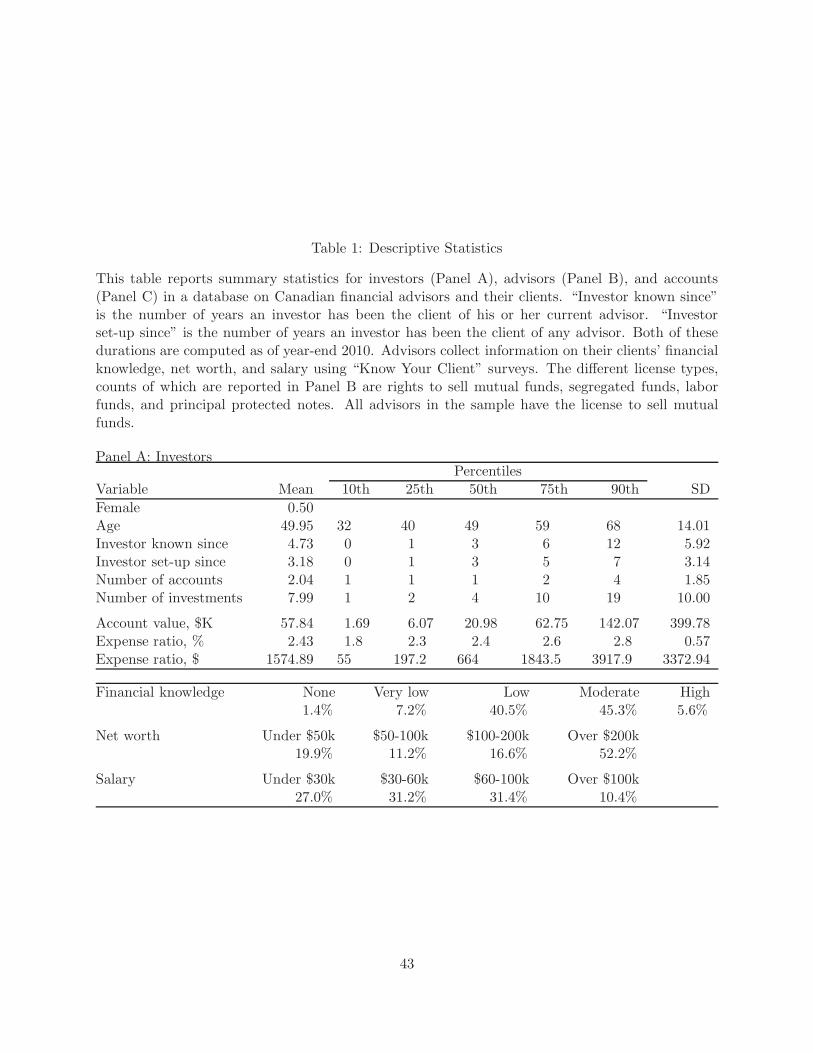
Table 1: Descriptive Statistics

This table reports summary statistics for investors (Panel A), advisors (Panel B), and accounts(Panel C) in a database on Canadian financial advisors and their clients. “Investor known since”is the number of years an investor has been the client of his or her current advisor. “Investorset-up since” is the number of years an investor has been the client of any advisor. Both of thesedurations are computed as of year-end 2010. Advisors collect information on their clients’ financialknowledge, net worth, and salary using “Know Your Client” surveys. The different license types,counts of which are reported in Panel B are rights to sell mutual funds, segregated funds, laborfunds, and principal protected notes. All advisors in the sample have the license to sell mutualfunds.

Panel A: InvestorsPercentiles

Variable Mean 10th 25th 50th 75th 90th SD

Female 0.50Age 49.95 32 40 49 59 68 14.01Investor known since 4.73 0 1 3 6 12 5.92Investor set-up since 3.18 0 1 3 5 7 3.14Number of accounts 2.04 1 1 1 2 4 1.85Number of investments 7.99 1 2 4 10 19 10.00

Account value, $K 57.84 1.69 6.07 20.98 62.75 142.07 399.78Expense ratio, % 2.43 1.8 2.3 2.4 2.6 2.8 0.57Expense ratio, $ 1574.89 55 197.2 664 1843.5 3917.9 3372.94

Financial knowledge None Very low Low Moderate High1.4% 7.2% 40.5% 45.3% 5.6%

Net worth Under $50k $50-100k $100-200k Over $200k19.9% 11.2% 16.6% 52.2%

Salary Under $30k $30-60k $60-100k Over $100k27.0% 31.2% 31.4% 10.4%

43

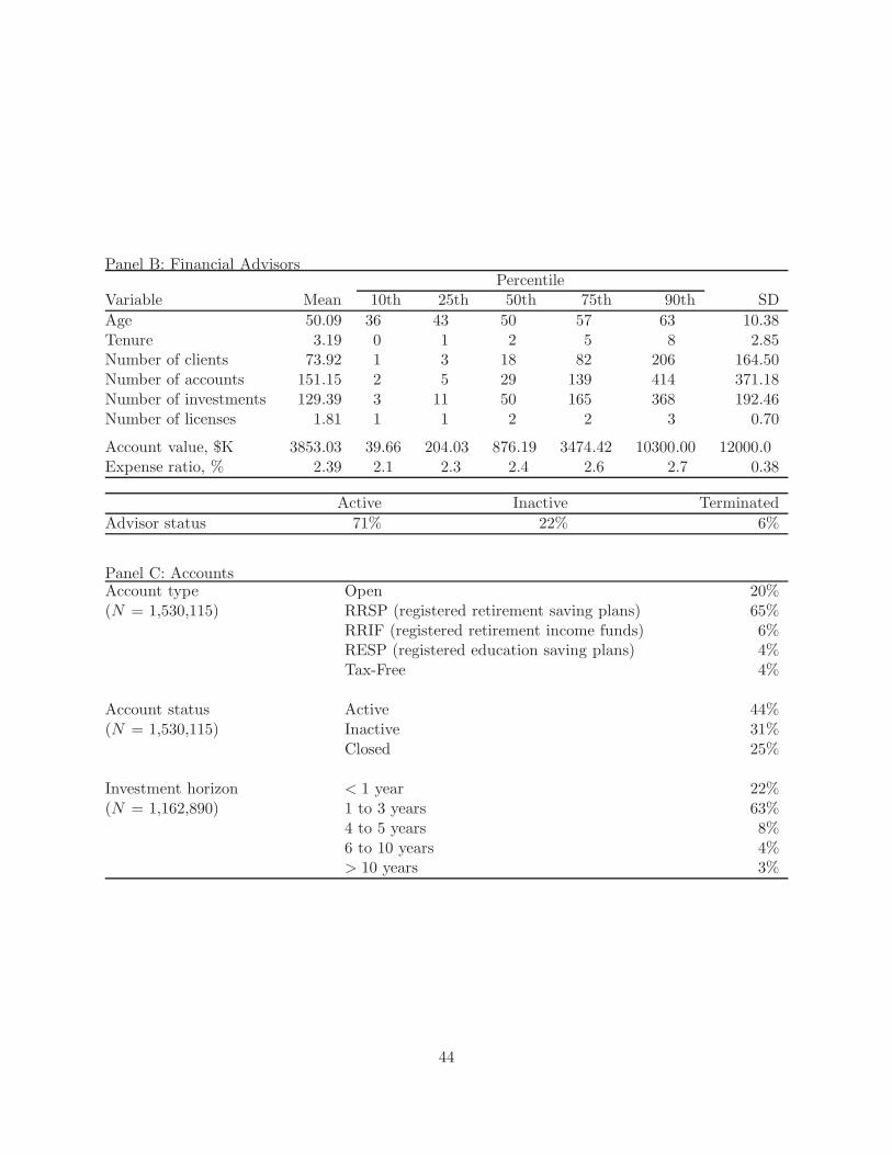
Panel B: Financial AdvisorsPercentile

Variable Mean 10th 25th 50th 75th 90th SD

Age 50.09 36 43 50 57 63 10.38Tenure 3.19 0 1 2 5 8 2.85Number of clients 73.92 1 3 18 82 206 164.50Number of accounts 151.15 2 5 29 139 414 371.18Number of investments 129.39 3 11 50 165 368 192.46Number of licenses 1.81 1 1 2 2 3 0.70

Account value, $K 3853.03 39.66 204.03 876.19 3474.42 10300.00 12000.0Expense ratio, % 2.39 2.1 2.3 2.4 2.6 2.7 0.38

Active Inactive Terminated

Advisor status 71% 22% 6%

Panel C: AccountsAccount type Open 20%(N = 1,530,115) RRSP (registered retirement saving plans) 65%

RRIF (registered retirement income funds) 6%RESP (registered education saving plans) 4%Tax-Free 4%

Account status Active 44%(N = 1,530,115) Inactive 31%

Closed 25%

Investment horizon < 1 year 22%(N = 1,162,890) 1 to 3 years 63%

4 to 5 years 8%6 to 10 years 4%> 10 years 3%

44

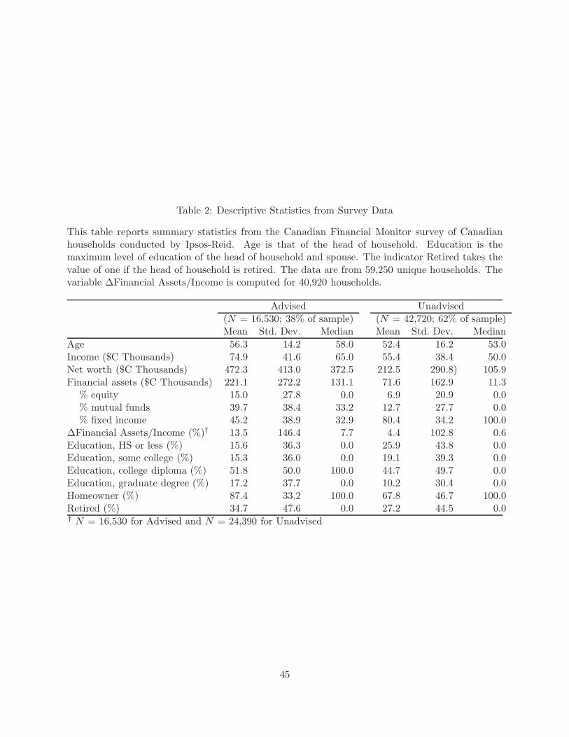
Table 2: Descriptive Statistics from Survey Data

This table reports summary statistics from the Canadian Financial Monitor survey of Canadianhouseholds conducted by Ipsos-Reid. Age is that of the head of household. Education is themaximum level of education of the head of household and spouse. The indicator Retired takes thevalue of one if the head of household is retired. The data are from 59,250 unique households. Thevariable ∆Financial Assets/Income is computed for 40,920 households.

Advised Unadvised(N = 16,530; 38% of sample) (N = 42,720; 62% of sample)Mean Std. Dev. Median Mean Std. Dev. Median

Age 56.3 14.2 58.0 52.4 16.2 53.0Income ($C Thousands) 74.9 41.6 65.0 55.4 38.4 50.0Net worth ($C Thousands) 472.3 413.0 372.5 212.5 290.8) 105.9Financial assets ($C Thousands) 221.1 272.2 131.1 71.6 162.9 11.3

% equity 15.0 27.8 0.0 6.9 20.9 0.0% mutual funds 39.7 38.4 33.2 12.7 27.7 0.0% fixed income 45.2 38.9 32.9 80.4 34.2 100.0

∆Financial Assets/Income (%)† 13.5 146.4 7.7 4.4 102.8 0.6Education, HS or less (%) 15.6 36.3 0.0 25.9 43.8 0.0Education, some college (%) 15.3 36.0 0.0 19.1 39.3 0.0Education, college diploma (%) 51.8 50.0 100.0 44.7 49.7 0.0Education, graduate degree (%) 17.2 37.7 0.0 10.2 30.4 0.0Homeowner (%) 87.4 33.2 100.0 67.8 46.7 100.0Retired (%) 34.7 47.6 0.0 27.2 44.5 0.0† N = 16,530 for Advised and N = 24,390 for Unadvised

45

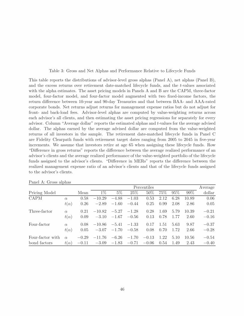
Table 3: Gross and Net Alphas and Performance Relative to Lifecycle Funds

This table reports the distributions of advisor-level gross alphas (Panel A), net alphas (Panel B),and the excess returns over retirement date-matched lifecycle funds, and the t-values associatedwith the alpha estimates. The asset pricing models in Panels A and B are the CAPM, three-factormodel, four-factor model, and four-factor model augmented with two fixed-income factors, thereturn difference between 10-year and 90-day Treasuries and that between BAA- and AAA-ratedcorporate bonds. Net returns adjust returns for management expense ratios but do not adjust forfront- and back-load fees. Advisor-level alphas are computed by value-weighting returns acrosseach advisor’s all clients, and then estimating the asset pricing regressions for separately for everyadvisor. Column “Average dollar” reports the estimated alphas and t-values for the average adviseddollar. The alphas earned by the average advised dollar are computed from the value-weightedreturns of all investors in the sample. The retirement date-matched lifecycle funds in Panel Care Fidelity Clearpath funds with retirement target dates ranging from 2005 to 2045 in five-yearincrements. We assume that investors retire at age 65 when assigning these lifecycle funds. Row“Difference in gross returns” reports the difference between the average realized performance of anadvisor’s clients and the average realized performance of the value-weighted portfolio of the lifecyclefunds assigned to the advisor’s clients. “Difference in MERs” reports the difference between therealized management expense ratio of an advisor’s clients and that of the lifecycle funds assignedto the advisor’s clients.

Panel A: Gross alphasPercentiles Average

Pricing Model Mean 1% 5% 25% 50% 75% 95% 99% dollar

CAPM α 0.58 −10.29 −4.88 −1.03 0.53 2.12 6.28 10.89 0.06t(α) 0.26 −2.89 −1.60 −0.44 0.25 0.99 2.08 2.86 0.05

Three-factor α 0.21 −10.82 −5.27 −1.28 0.28 1.69 5.79 10.39 −0.21t(α) 0.09 −3.10 −1.67 −0.56 0.13 0.78 1.77 2.60 −0.16

Four-factor α 0.08 −10.86 −5.41 −1.33 0.17 1.51 5.63 9.87 −0.37t(α) 0.05 −3.07 −1.70 −0.58 0.08 0.70 1.72 2.66 −0.28

Four-factor with α −0.29 −11.76 −6.26 −1.70 −0.13 1.22 5.10 10.56 −0.54bond factors t(α) −0.11 −3.09 −1.83 −0.71 −0.06 0.54 1.49 2.43 −0.40

46

Panel B: Net alphas (after MERs)Percentiles Average

Pricing Model Mean 1% 5% 25% 50% 75% 95% 99% dollar

CAPM α −1.83 −13.01 −7.35 −3.40 −1.86 −0.29 3.81 8.46 −2.31t(α) −0.87 −4.31 −2.71 −1.57 −0.88 −0.12 1.15 1.90 −1.75

Three-factor α −2.21 −13.60 −7.73 −3.66 −2.11 −0.74 3.38 7.99 −2.59t(α) −1.02 −4.36 −2.77 −1.69 −1.03 −0.32 0.93 1.79 −1.91

Four-factor α −2.34 −13.59 −7.89 −3.74 −2.22 −0.92 3.19 7.47 −2.74t(α) −1.07 −4.34 −2.80 −1.73 −1.09 −0.40 0.90 1.78 −2.04

Four-factor with α −2.70 −14.39 −8.59 −4.08 −2.52 −1.22 2.70 8.26 −2.91bond factors t(α) −1.20 −4.43 −2.96 −1.87 −1.22 −0.51 0.69 1.58 −2.13

Panel C: Realized returns over retirement date-matched lifecycle funds

Percentiles AverageDifference in: Mean 1% 5% 25% 50% 75% 95% 99% dollar

Gross returns −0.41 −20.28 −8.48 −2.36 −0.47 1.33 7.98 19.53 −0.87

MERs 1.33 0.03 0.70 1.18 1.35 1.51 1.81 2.48 1.31

47

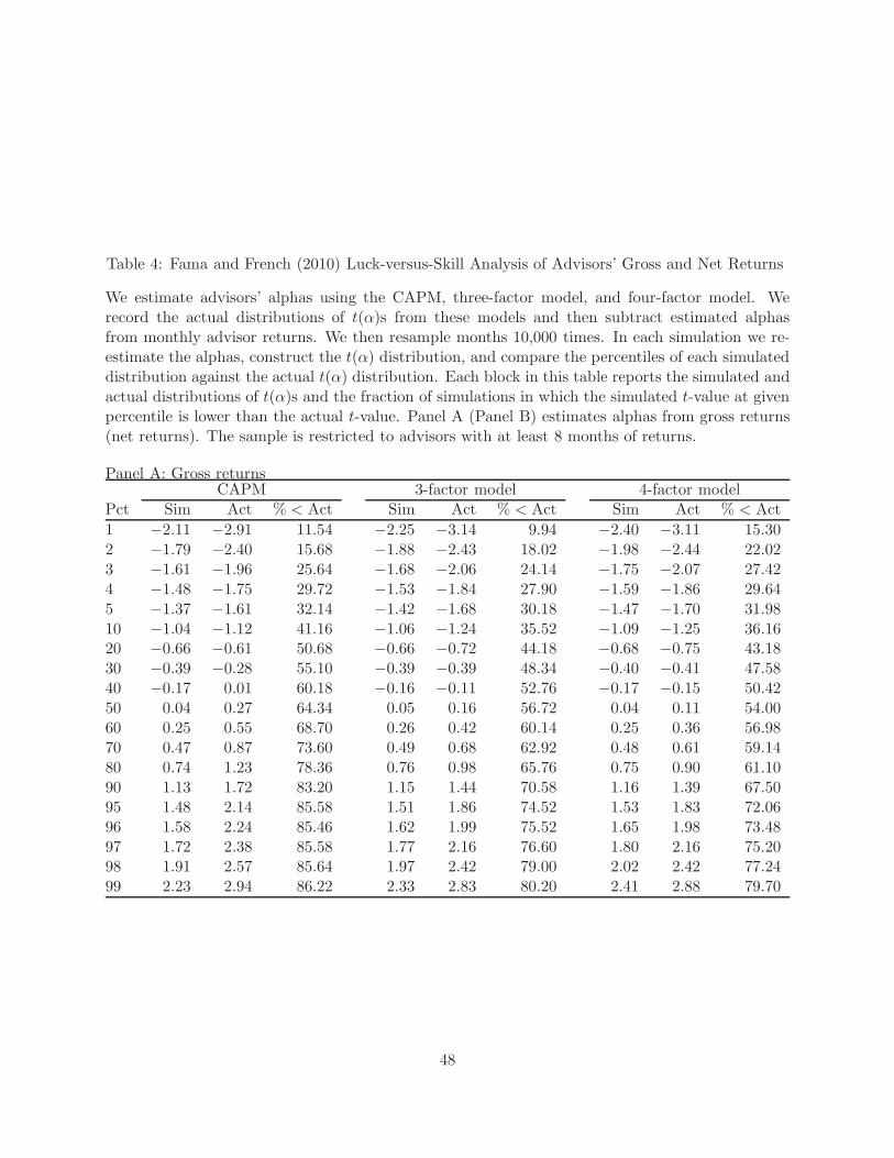
Table 4: Fama and French (2010) Luck-versus-Skill Analysis of Advisors’ Gross and Net Returns

We estimate advisors’ alphas using the CAPM, three-factor model, and four-factor model. Werecord the actual distributions of t(α)s from these models and then subtract estimated alphasfrom monthly advisor returns. We then resample months 10,000 times. In each simulation we re-estimate the alphas, construct the t(α) distribution, and compare the percentiles of each simulateddistribution against the actual t(α) distribution. Each block in this table reports the simulated andactual distributions of t(α)s and the fraction of simulations in which the simulated t-value at givenpercentile is lower than the actual t-value. Panel A (Panel B) estimates alphas from gross returns(net returns). The sample is restricted to advisors with at least 8 months of returns.

Panel A: Gross returnsCAPM 3-factor model 4-factor model

Pct Sim Act % < Act Sim Act % < Act Sim Act % < Act

1 −2.11 −2.91 11.54 −2.25 −3.14 9.94 −2.40 −3.11 15.302 −1.79 −2.40 15.68 −1.88 −2.43 18.02 −1.98 −2.44 22.023 −1.61 −1.96 25.64 −1.68 −2.06 24.14 −1.75 −2.07 27.424 −1.48 −1.75 29.72 −1.53 −1.84 27.90 −1.59 −1.86 29.645 −1.37 −1.61 32.14 −1.42 −1.68 30.18 −1.47 −1.70 31.9810 −1.04 −1.12 41.16 −1.06 −1.24 35.52 −1.09 −1.25 36.1620 −0.66 −0.61 50.68 −0.66 −0.72 44.18 −0.68 −0.75 43.1830 −0.39 −0.28 55.10 −0.39 −0.39 48.34 −0.40 −0.41 47.5840 −0.17 0.01 60.18 −0.16 −0.11 52.76 −0.17 −0.15 50.4250 0.04 0.27 64.34 0.05 0.16 56.72 0.04 0.11 54.0060 0.25 0.55 68.70 0.26 0.42 60.14 0.25 0.36 56.9870 0.47 0.87 73.60 0.49 0.68 62.92 0.48 0.61 59.1480 0.74 1.23 78.36 0.76 0.98 65.76 0.75 0.90 61.1090 1.13 1.72 83.20 1.15 1.44 70.58 1.16 1.39 67.5095 1.48 2.14 85.58 1.51 1.86 74.52 1.53 1.83 72.0696 1.58 2.24 85.46 1.62 1.99 75.52 1.65 1.98 73.4897 1.72 2.38 85.58 1.77 2.16 76.60 1.80 2.16 75.2098 1.91 2.57 85.64 1.97 2.42 79.00 2.02 2.42 77.2499 2.23 2.94 86.22 2.33 2.83 80.20 2.41 2.88 79.70

48

Panel B: Net returnsCAPM 3-factor model 4-factor model

Pct Sim Act % < Act Sim Act % < Act Sim Act % < Act

1 −2.11 −4.34 0.18 −2.25 −4.43 0.50 −2.40 −4.45 1.662 −1.79 −3.57 0.40 −1.88 −3.56 0.80 −1.98 −3.59 1.603 −1.61 −3.11 0.98 −1.68 −3.15 1.16 −1.75 −3.19 1.584 −1.48 −2.87 1.40 −1.53 −2.94 1.14 −1.59 −2.96 1.705 −1.38 −2.71 1.64 −1.42 −2.77 1.46 −1.47 −2.78 1.8810 −1.04 −2.20 3.42 −1.06 −2.31 2.18 −1.09 −2.34 2.4220 −0.66 −1.73 4.72 −0.66 −1.84 3.14 −0.68 −1.86 3.1430 −0.39 −1.39 6.22 −0.39 −1.51 3.88 −0.40 −1.56 3.7840 −0.17 −1.13 6.84 −0.16 −1.24 4.54 −0.17 −1.29 4.3050 0.04 −0.84 8.46 0.05 −0.99 5.10 0.04 −1.04 4.7260 0.25 −0.57 10.32 0.26 −0.71 5.84 0.25 −0.79 5.0270 0.47 −0.24 13.66 0.48 −0.42 6.88 0.48 −0.49 5.8080 0.74 0.16 19.38 0.76 −0.02 9.90 0.75 −0.10 7.7690 1.13 0.80 32.50 1.15 0.59 18.42 1.16 0.55 15.9295 1.48 1.26 39.42 1.51 1.11 28.18 1.53 1.07 24.4096 1.58 1.39 41.06 1.62 1.23 27.98 1.65 1.20 25.1697 1.72 1.51 40.36 1.77 1.39 29.40 1.80 1.37 26.5098 1.91 1.69 40.68 1.97 1.62 31.64 2.02 1.64 30.7299 2.23 2.01 40.74 2.34 1.94 29.90 2.42 2.05 33.12

49

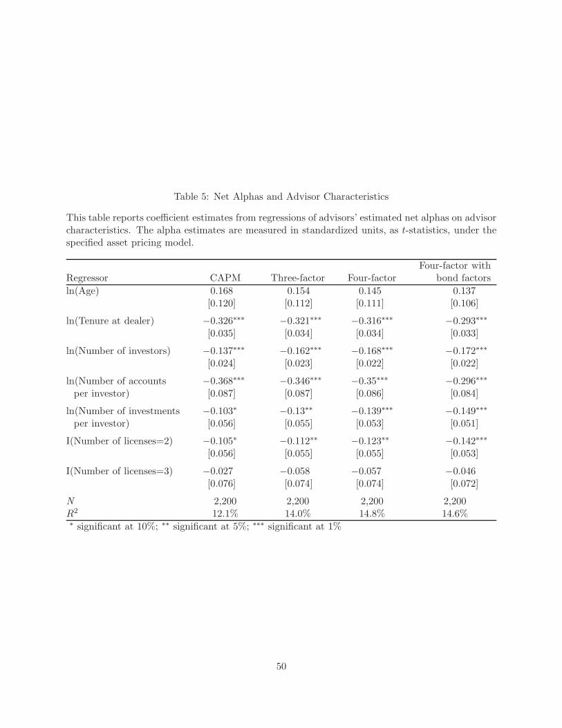
Table 5: Net Alphas and Advisor Characteristics

This table reports coefficient estimates from regressions of advisors’ estimated net alphas on advisorcharacteristics. The alpha estimates are measured in standardized units, as t-statistics, under thespecified asset pricing model.

Four-factor withRegressor CAPM Three-factor Four-factor bond factors

ln(Age) 0.168 0.154 0.145 0.137[0.120] [0.112] [0.111] [0.106]

ln(Tenure at dealer) −0.326∗∗∗ −0.321∗∗∗ −0.316∗∗∗ −0.293∗∗∗

[0.035] [0.034] [0.034] [0.033]

ln(Number of investors) −0.137∗∗∗ −0.162∗∗∗ −0.168∗∗∗ −0.172∗∗∗

[0.024] [0.023] [0.022] [0.022]

ln(Number of accounts −0.368∗∗∗ −0.346∗∗∗ −0.35∗∗∗ −0.296∗∗∗

per investor) [0.087] [0.087] [0.086] [0.084]

ln(Number of investments −0.103∗ −0.13∗∗ −0.139∗∗∗ −0.149∗∗∗

per investor) [0.056] [0.055] [0.053] [0.051]

I(Number of licenses=2) −0.105∗ −0.112∗∗ −0.123∗∗ −0.142∗∗∗

[0.056] [0.055] [0.055] [0.053]

I(Number of licenses=3) −0.027 −0.058 −0.057 −0.046[0.076] [0.074] [0.074] [0.072]

N 2,200 2,200 2,200 2,200R2 12.1% 14.0% 14.8% 14.6%∗ significant at 10%; ∗∗ significant at 5%; ∗∗∗ significant at 1%

50

Table 6: Account Closure and Past Performance

This table reports estimates from Cox proportional hazards rate models with time-varying covari-ates that examine how the probability that an investor closes his account is related to her pastperformance over the prior one-year period (Panel A) or the average expense ratio of the investorsholding over the prior one-year period (Panel B). The first model has only the prior one-year re-turn (or expense ratio) as the covariate; the second model adds year-month fixed effects; and thethird model replaces the prior one-year return (or expense ratio) with dummy variables to rep-resent different intervals of performance or fees. t-values are reported in parentheses. The dataused for estimation contain 64,750 investors, 19,977 account closures, and 3,542,907 investor-monthobservations.

Panel A: One-year returns as time-varying covariates

ModelCovariate (1) (2) (3)

Realized returnt−12,t 0.76 0.98(−5.31) (−0.23)

Return-category dummy variables:<Realized returnt−12,t ≤ -30% 1.05

(0.73)-30% < Realized returnt−12,t ≤ 20% 1.09

(1.64)-20% < Realized returnt−12,t ≤ 10% 1.18

(4.27)-10% < Realized returnt−12,t ≤ 0% 1.33

(10.40)0% < Realized returnt−12,t ≤ 10% Omitted

10% < Realized returnt−12,t ≤ 20% 1.03(1.23)

20% < Realized returnt−12,t ≤ 30% 0.97(−0.71)

30% < Realized returnt−12,t≤ 1.13(2.11)

Year-month FE No Yes Yes

51

Panel B: One-year expense ratios as time-varying covariatesSample

Low High or moderatefinancial financial

All clients knowledge knowledgeRegressor (1) (2) (3)

Expense ratiot−12,t 1.18 0.97 1.45

(3.13) (−0.33) (4.46)

Control for risky asset share? Yes Yes Yes

52

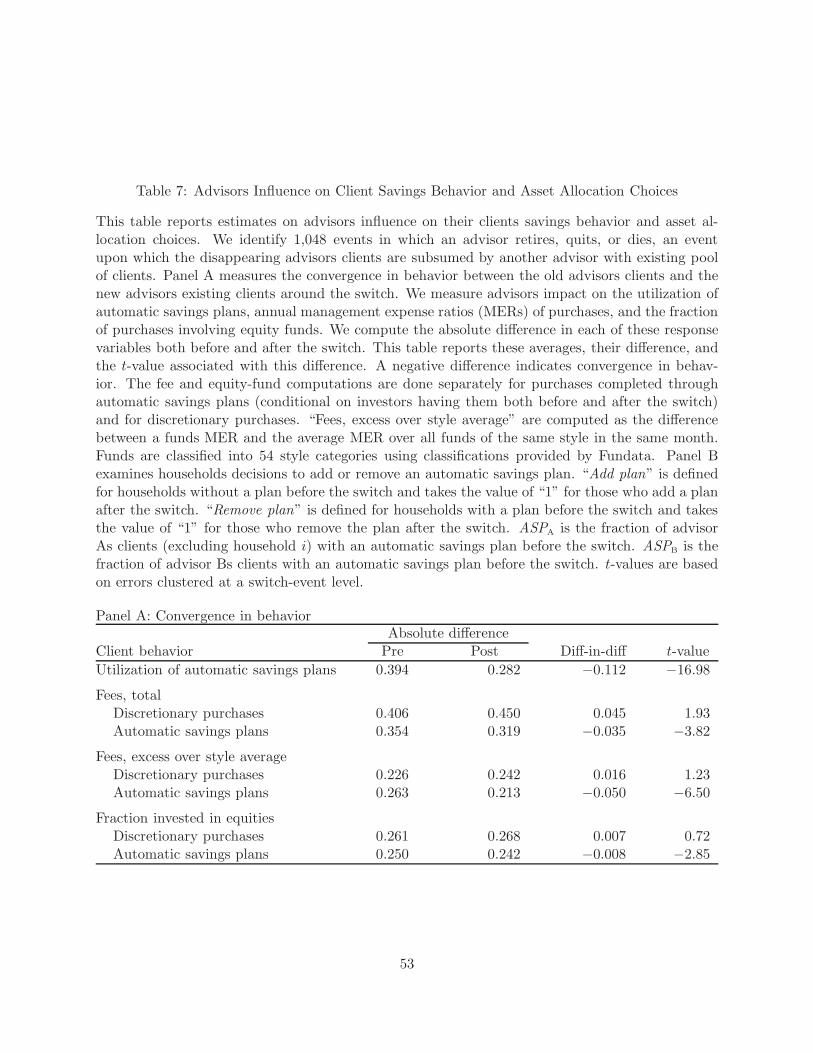
Table 7: Advisors Influence on Client Savings Behavior and Asset Allocation Choices

This table reports estimates on advisors influence on their clients savings behavior and asset al-location choices. We identify 1,048 events in which an advisor retires, quits, or dies, an eventupon which the disappearing advisors clients are subsumed by another advisor with existing poolof clients. Panel A measures the convergence in behavior between the old advisors clients and thenew advisors existing clients around the switch. We measure advisors impact on the utilization ofautomatic savings plans, annual management expense ratios (MERs) of purchases, and the fractionof purchases involving equity funds. We compute the absolute difference in each of these responsevariables both before and after the switch. This table reports these averages, their difference, andthe t-value associated with this difference. A negative difference indicates convergence in behav-ior. The fee and equity-fund computations are done separately for purchases completed throughautomatic savings plans (conditional on investors having them both before and after the switch)and for discretionary purchases. “Fees, excess over style average” are computed as the differencebetween a funds MER and the average MER over all funds of the same style in the same month.Funds are classified into 54 style categories using classifications provided by Fundata. Panel Bexamines households decisions to add or remove an automatic savings plan. “Add plan” is definedfor households without a plan before the switch and takes the value of “1” for those who add a planafter the switch. “Remove plan” is defined for households with a plan before the switch and takesthe value of “1” for those who remove the plan after the switch. ASPA is the fraction of advisorAs clients (excluding household i) with an automatic savings plan before the switch. ASPB is thefraction of advisor Bs clients with an automatic savings plan before the switch. t-values are basedon errors clustered at a switch-event level.

Panel A: Convergence in behaviorAbsolute difference

Client behavior Pre Post Diff-in-diff t-value

Utilization of automatic savings plans 0.394 0.282 −0.112 −16.98

Fees, totalDiscretionary purchases 0.406 0.450 0.045 1.93Automatic savings plans 0.354 0.319 −0.035 −3.82

Fees, excess over style averageDiscretionary purchases 0.226 0.242 0.016 1.23Automatic savings plans 0.263 0.213 −0.050 −6.50

Fraction invested in equitiesDiscretionary purchases 0.261 0.268 0.007 0.72Automatic savings plans 0.250 0.242 −0.008 −2.85

53

Panel B: Decision to add or remove an automatic savings planDependent variable

Add plan Remove plan

I(ASPB > ASPA) 0.017 0.002(2.91) (0.52)

ASPB − ASPA 0.033 0.026 −0.002 −0.002(3.31) (2.88) (−0.37) (−0.19)

I(ASPB > ASPA) ∗ (ASPB − ASPA) 0.018 −0.001(0.57) (−0.05)

Adjusted R2 0.20% 0.26% 0.27% 0.00% 0.00% 0.00%

54

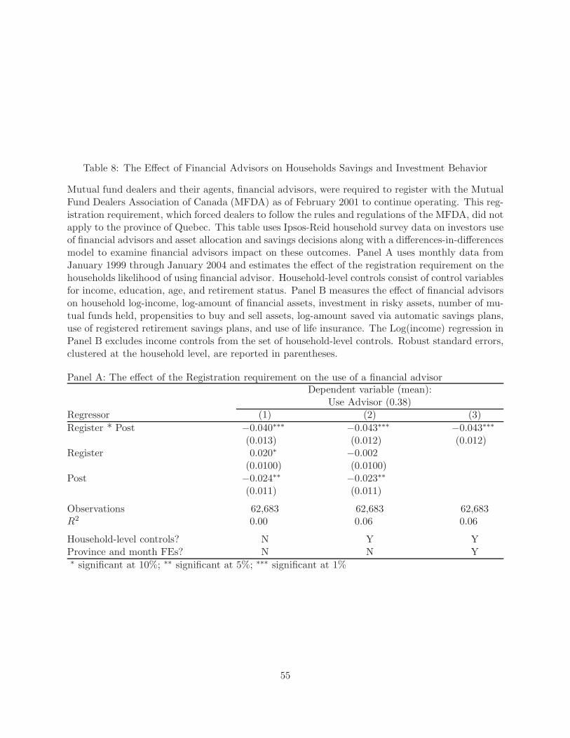
Table 8: The Effect of Financial Advisors on Households Savings and Investment Behavior

Mutual fund dealers and their agents, financial advisors, were required to register with the MutualFund Dealers Association of Canada (MFDA) as of February 2001 to continue operating. This reg-istration requirement, which forced dealers to follow the rules and regulations of the MFDA, did notapply to the province of Quebec. This table uses Ipsos-Reid household survey data on investors useof financial advisors and asset allocation and savings decisions along with a differences-in-differencesmodel to examine financial advisors impact on these outcomes. Panel A uses monthly data fromJanuary 1999 through January 2004 and estimates the effect of the registration requirement on thehouseholds likelihood of using financial advisor. Household-level controls consist of control variablesfor income, education, age, and retirement status. Panel B measures the effect of financial advisorson household log-income, log-amount of financial assets, investment in risky assets, number of mu-tual funds held, propensities to buy and sell assets, log-amount saved via automatic savings plans,use of registered retirement savings plans, and use of life insurance. The Log(income) regression inPanel B excludes income controls from the set of household-level controls. Robust standard errors,clustered at the household level, are reported in parentheses.

Panel A: The effect of the Registration requirement on the use of a financial advisorDependent variable (mean):

Use Advisor (0.38)Regressor (1) (2) (3)

Register * Post −0.040∗∗∗ −0.043∗∗∗ −0.043∗∗∗

(0.013) (0.012) (0.012)Register 0.020∗ −0.002

(0.0100) (0.0100)Post −0.024∗∗ −0.023∗∗

(0.011) (0.011)

Observations 62,683 62,683 62,683R2 0.00 0.06 0.06

Household-level controls? N Y YProvince and month FEs? N N Y∗ significant at 10%; ∗∗ significant at 5%; ∗∗∗ significant at 1%

55

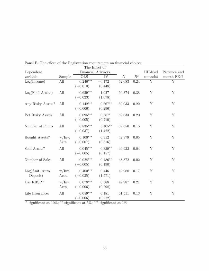
Panel B: The effect of the Registration requirement on financial choicesThe Effect of

Dependent Financial Advisors HH-level Province andvariable Sample OLS IV N R2 controls? month FEs?

Log(Income) All 0.246∗∗∗ −0.172 62,683 0.24 Y Y(−0.010) (0.448)

Log(Fin’l Assets) All 0.659∗∗∗ 1.027 60,374 0.38 Y Y(−0.023) (1.078)

Any Risky Assets? All 0.142∗∗∗ 0.667∗∗ 59,033 0.22 Y Y(−0.006) (0.296)

Pct Risky Assets All 0.095∗∗∗ 0.387∗ 59,033 0.20 Y Y(−0.005) (0.210)

Number of Funds All 0.835∗∗∗ 3.405∗∗ 59,650 0.15 Y Y(−0.037) (1.422)

Bought Assets? w/Inv. 0.100∗∗∗ 0.352 42,979 0.05 Y YAcct. (−0.007) (0.316)

Sold Assets? All 0.045∗∗∗ 0.339∗∗ 46,932 0.04 Y Y(−0.005) (0.157)

Number of Sales All 0.028∗∗∗ 0.486∗∗ 48,872 0.02 Y Y(−0.005) (0.190)

Log(Amt. Auto w/Inv. 0.400∗∗∗ 0.446 42,988 0.17 Y YDeposit) Acct. (−0.035) (1.571)

Use RRSP? w/Inv. 0.078∗∗∗ 0.388 42,987 0.21 Y YAcct. (−0.006) (0.298)

Life Insurance? All 0.059∗∗∗ 0.181 61,511 0.13 Y Y(−0.006) (0.272)

∗ significant at 10%; ∗∗ significant at 5%; ∗∗∗ significant at 1%

56

Table A1: Correlations in Trading Flows

This table reports estimates from regressions of investors buy-sell ratios on the buy-sell ratios of allother clients of the same advisor (“co-clients buy-sell ratio”) and the clients of all other advisors(“other clients buy-sell ratio”). Buy-sell ratio is as the value of purchases minus the value of salesdivided by the total value of purchases and sales. Each observation is an investor-month-fundtriplet. t-values are reported in parentheses.

Dependent variable: Buy-sell ratio(1) (2) (3)

Co-clients’ buy-sell ratio 0.158 0.142 0.140(27.39) (27.28) (26.09)

Other clients’ buy-sell ratio 0.030 0.018 0.019(18.47) (19.26) (15.42)

Additional client controls No No Yes(age, gender, relationshiplongevity, account longevity)

Additional advisor controls No No Yes(age, license longevity,tenure, number of licenses)

Fund fixed effects No Yes Yes

N 78,215,376 78,215,376 14,276,642Adjusted R2 6.7% 6.7% 10.2%

57

Table A2: Correlations in Trading Flows by Plan Type and Investment Horizon

This table reports estimates from regressions of investors buy-sell ratios on the buy-sell ratiosof all other clients of the same advisor (“co-clients buy-sell ratio”) and the clients of all otheradvisors (“other clients buy-sell ratio”). Each model is estimated on a separate sub-sample ofclient accounts, splitting first by the investment plan type and then by the clients self-reportedinvestment horizon. All models include fund fixed effects and the full set of controls for investorand advisor demographics.

Plan type Co-clients Other clients N

Open 0.073∗∗∗ 0.024∗∗∗ 2,099,735Registered retirement saving plans 0.140∗∗∗ 0.028∗∗∗ 10,002,536Registered retirement income plans 0.110∗∗∗ −0.003 1,937,611Registered education savings plans 0.087∗∗∗ 0.019∗∗∗ 481,360Tax-free 0.110∗∗∗ 0.035∗∗∗ 113,845

Investment horizon Co-clients Other clients N

Less than a year 0.140∗∗∗ 0.013∗∗∗ 504,5161-3 years 0.110∗∗∗ 0.025∗∗∗ 227,2504-5 years 0.110∗∗∗ 0.021∗∗∗ 561,5756-10 years 0.140∗∗∗ 0.020∗∗∗ 11,339,404Over 10 years 0.130∗∗∗ 0.022∗∗∗ 900,165∗ significant at 10%; ∗∗ significant at 5%; ∗∗∗ significant at 1%

58