the crime reduction effects of public cctv … crime reduction effects of public cctv cameras: a...

JUSTICE QUARTERLY VOLUME 26 NUMBER 4 (DECEMBER 2009)

ISSN 0741-8825 print/1745-9109 online/09/040746-25© 2009 Academy of Criminal Justice SciencesDOI: 10.1080/07418820902873852

The Crime Reduction Effects of Public CCTV Cameras: A Multi-Method Spatial Approach

Jerry H. Ratcliffe, Travis Taniguchi and Ralph B. Taylor

Taylor and FrancisRJQY_A_387557.sgm10.1080/07418820902873852Justice Quarterly0741-8825 (print)/1745-9109 (online)Original Article2009Taylor & [email protected]

Public Closed Circuit TeleVision (CCTV) initiatives have been utilized as methodsof monitoring public space for over two decades. Evaluations of these efforts toreduce crime have been mixed. Furthermore, there has been a paucity of rigor-ous evaluations of cameras located in the USA. In this analysis, crime in theviewshed of publicly funded CCTV cameras in Philadelphia, PA, is examinedusing two evaluation techniques: hierarchical linear modeling and weighteddisplacement quotients. An analysis that incorporates controls for long-termtrends and seasonality finds that the introduction of cameras is associated witha 13% reduction in crime. The evaluation suggests that while there appears tobe a general benefit to the cameras, there were as many sites that showed nobenefit of camera presence as there were locations with a positive outcome oncrime. The policy implications of these findings are discussed.

Keywords CCTV; video surveillance; repeated measures; hierarchical linearmodeling; weighted displacement quotients; Philadelphia

Introduction

Closed Circuit Television (CCTV) seeks to reduce crime primarily by increasingthe perception among potential offenders that there is an increased risk of

Jerry Ratcliffe is a Professor in the Department of Criminal Justice at Temple University. Recentbooks have included Intelligence-Led Policing, and Strategic Thinking in Criminal Intelligence(second edition). Further details are online at jratcliffe.net. Travis Taniguchi is a doctoral candidatein the Department of Criminal Justice at Temple University. His publications can be found in JusticeQuarterly and Crime Patterns & Analysis. Ralph B. Taylor is a Professor in the Department ofCriminal Justice at Temple University. Research interests include incivilities, communities andcrime, reactions to crime, guns, juries, and DNA policies. Publications are listed online atwww.rbtaylor.net/pubs.htm. Correspondence to: Jerry H. Ratcliffe, Department of Criminal Justice,Temple University, 1115 W. Berks Street, Philadelphia, PA 19122, USA. E-mail: [email protected]

Downloaded By: [Ratcliffe, Jerry] At: 12:55 14 October 2009

EVALUATING PHILADELPHIA CCTV 747

detection and capture (Ratcliffe, 2006). Proponents of CCTV argue thatincreased surveillance will reduce crime and increase arrests of offenders, whileopponents lament the invasion of privacy in public areas and point to researchfindings that are less than definitive. Irrespective of the theoretical validity ofthe crime prevention role of CCTV systems, the growth of CCTV schemes acrossnumerous countries (including the USA) has been substantial. The history ofCCTV technology is one of rapid evolution from static, low-resolution camerasto high quality technology solutions that can pan, tilt, and zoom at thecommand (through either wireless interface or fiber optic cable) of remoteoperators connected to a police radio network. This implementation and tech-nological expansion of CCTV schemes has, until recently, taken place in an envi-ronment largely devoid of rigorous evaluation of the effectiveness of CCTV toprevent crime (see Welsh & Farrington, 2007, for a comprehensive review).

The emergence of CCTV has taken place during a period when crime analysishas improved in resolution (both spatial and temporal) enabling academicresearch and practitioner focus to become more place-specific rather thangeneralized to the neighborhood level (Mazerolle, Hurley, & Chamlin, 2002),and during a period that has seen the rise of problem-oriented policing (Clarke,2004; Goldstein, 2003) as an operational strategy that can capitalize on theanalytical improvements available. Intelligence-led policing has provided a busi-ness model to coordinate crime detection and prevention activities, throughwhich problem-oriented policing can flow in an operational environment (Ratc-liffe, 2008). From the earliest wide-scale implementation of CCTV technology inBritain in the 1980s, however, the assessment of CCTV schemes has been signif-icantly hampered on two fronts. Numerous well-meaning evaluations havelacked either an impartial perspective and/or methodological rigor. For exam-ple, many have been either conducted by city agencies or technology companiesinvolved in the scheme and whom may be perceived to have vested interests inthe evaluation outcomes; or, like the earliest independent evaluation of a CCTVimplementation from King’s Lynn, UK (Brown, 1995)—where 19 cameras wereinstalled at public car parks across the city—had methodological limitations dueto a lack of controls for seasonality or long-term temporal trends. Numerousother studies since King’s Lynn have lacked measures of control areas, controlsfor seasonal variation, or have been absent of any indicators of potentialdisplacement (or diffusion of benefits).

Furthermore, the existing evaluation literature demonstrates considerablevariation in not only methodology, but also outcome measures and independentvariables. Some studies examine the impact of cameras on crime within adefined distance of CCTV cameras (Harada, Yonezato, Suzuki, Shimada, Era, &Saito, 2004), while others surveyed residents in camera areas for their percep-tions of how crime has changed (Squires, 2003). Other studies have interviewedkey stakeholders (Hood, 2003) or examined emergency room attendance levelsrelated to assaults (Sivarajasingam, Shepherd, & Matthews, 2003).

Welsh and Farrington’s (2007) systematic review identified four essentialcriteria for inclusion in their study:


748 RATCLIFFE ET AL.

(1) CCTV was the main intervention examined;(2) the outcome measure was crime;(3) the evaluation had a minimum methodological design that incorporated at

least before-and-after measures of crime in experimental and comparablecontrol areas; and

(4) there was a minimum number of crimes (20) recorded in the experimentalarea prior to the CCTV implementation.

Even within this basic evaluation criteria framework, Welsh and Farrington(2007) had to exclude numerous studies because they lacked appropriate andcomparable control areas. They were able to identify 44 relevant studies, butonly 22 that were applicable to city centers and public urban areas. Of these 22studies, 17 were conducted in the UK, two in Scandinavia, and three from theUSA; however, the three from the USA were actually at three locations inCincinnati, Ohio, and were reported in a single journal article (Mazerolle et al.,2002).1

Given the scarcity of CCTV evaluations in the USA, the study conducted byMazerolle et al. (2002) is worth discussing in some depth both because of itsinnovations and its limitations. This study utilized a multi-method approach toevaluating the CCTV initiative in Cincinnati, Ohio. First, they used an innovativemethod to measure both pro- and anti-social behavior in the vicinity of thecamera locations. The researchers reviewed random samples of video capturedby the cameras and coded activity along a number of dimensions including: thequality of image being recorded, the number of people and vehicles at thetarget site, and a range of pro-social (e.g., pedestrian traffic and people shop-ping) and anti-social (such as people loitering, dealing drugs, or begging) behav-iors. Use of interrupted time series models found a complicated relationshipbetween the implementation of cameras and their crime deterrence effects.The second evaluation method evaluated the change in calls for service (notrecorded crime) in the areas surrounding CCTV target sites. Overall, it wasconcluded that the implementation of CCTV systems produced an initial deter-rence effect in the one to two months following implementation. This crimesuppressing effect, however, seemed to decline as people adapted to cameraplacement. While the study conducted by Lorraine Mazerolle and colleagues ismethodologically sound and empirically sophisticated, there are a number oflimitations that are worth addressing. First, the use of calls for service ratherthan recorded crime basically means that there has not been a single study ofCCTV in America that uses recorded crime as an outcome measure in a mannerthat satisfies Welsh and Farrington’s (2007) systematic review criteria. Second,the authors utilized circular buffers surrounding the camera target areas. Theseuniform buffers are not sensitive to the actual viewsheds of the cameras. It ispossible that these buffers are both over-inclusive and under-inclusive of areas

1. There have also been two US studies that examined CCTV in public housing complexes. These arediscussed in Welsh and Farrington (2007).



where cameras may have a crime deterrent effect. Finally, Mazerolle et al(2002) do not consider the possible displacement effects of camera implementa-tion. The current evaluation attempts to rectify these limitations.

The lack of evaluation research seems a significant omission on the part ofthe research community given the growing enthusiasm across America for CCTV.While there are no national estimates on the extent of CCTV across America,newspaper accounts suggest that CCTV cameras are being implemented at asignificant rate. For example, San Francisco has spent close to $1m on 74cameras at 25 locations, and a further 25 cameras are planned (Bulwa, 2008);and Washington, DC plans a $4.5 million expansion of its surveillance system(Klein, 2008). This rapid and unprecedented expansion of video surveillancetechnology is not just limited to the major urban areas (Welsh & Farrington,2007). Reductions in technology cost and a perception that CCTV is a cost-effective crime prevention tool, have driven investment in video surveillance inmunicipal areas across America.

For all this enthusiasm for video surveillance, there has been a lack of highquality, independent evaluation studies (Eck, 1997). Using Hierarchical LinearModeling (HLM) and Weighed Displacement Quotient (WDQ) methodologies, weexplore serious crime, disorder crime, and an all-crime measure combining seriouscrime and disorder, with a multi-method spatio-temporal evaluation of 18 pilotCCTV cameras across 10 sites in Philadelphia, PA.

Data

Camera types, locations, and implementation details

The Philadelphia pilot project employed two different camera types. Eight pan,tilt, zoom (PTZ) cameras were installed between July 2006 and October 2006.These cameras have the capacity to tilt up and down, pan around the surround-ing area, and zoom. Examination of the zoom capacity by the researchers indi-cated that the camera allows the police officer to read a car license plate morethan a block away, and observe street activity up to three blocks distance, ifthe view is unobstructed. The video feed is routed directly to police headquar-ters where a police officer monitors all PTZ cameras in real time. The imagesare also recorded digitally, with a hard drive storage capacity sufficient to storeimages for 12 days.

The remaining 10 cameras did not allow for live monitoring. The PortableOvert Digital Surveillance System (PODSS) cameras, as implemented in Philadel-phia, provide a moveable, self-contained digital camera and recording systemthat is housed in a bullet-resistant unit with flashing strobe lights to draw theattention of the public and potential offenders. The cameras are visually quitedifferent from the PTZ cameras, being housed in a much larger and more visibleunit. As implemented in Philadelphia, these cameras are not monitored atpolice headquarters; however, nearby patrol officers with the correct



equipment in two-officer cars can theoretically view the feed from camerasover a wireless link (though the senior officer in charge of implementation didnot believe this took place on any regular basis). The system is also able torecord up to five days of street activity on a digital hard drive. When a crime issuspected to have occurred within the view of the camera, a police officermeets street engineering personnel from the city and the digital video recordhard drive is retrieved from the unit with the aid of a crane. Discussions withpolice officers suggested that the whole process can take up to two hours.

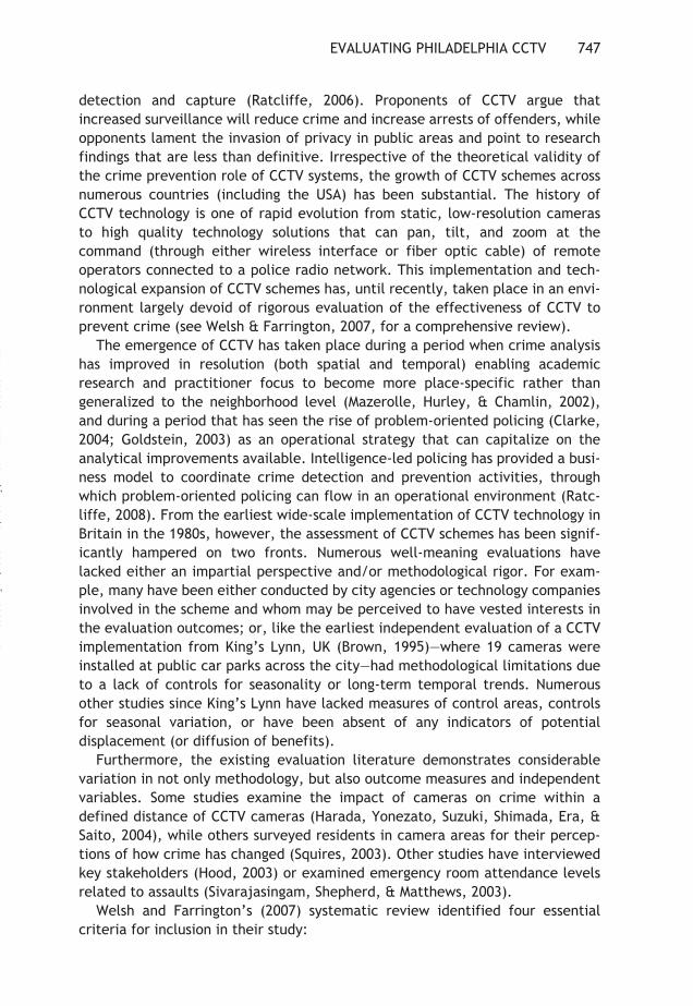
Although there are a total of 18 cameras at 12 locations, some cameras arelocated so close to other cameras (within a block’s distance) that the decision

Figure 1 Pilot project camera locations in Philadelphia, PA.



was made to evaluate spatial sites rather than individual cameras. The situationis further complicated by cameras three to five which are not located at a singlesite but are close enough that any potential displacement would likely be tooverlapping areas. Therefore, we collapsed sites three to five into a single loca-tion leaving eight different evaluation areas, labeled 1, 2, 3–5, 6, 7, 8, 9, 10 onFigure 1. The choice of camera was dictated by the locational demands of thearea, and was made by Philadelphia Police Department (PPD) officers prior toour involvement in the project.Figure 1 Pilot project camera locations in Philadelphia, PA.

Offender perception or camera viewshed?

It can be argued (e.g., Ratcliffe, 2006) that from a rational choice perspective(Clarke & Felson, 1993; Cornish & Clarke, 1986; Jeffery & Zahm, 1993) comesthe supposition that cameras may work to prevent crime if two criteria are met:the offender is aware that the camera may be monitoring their activity, and theoffender perceives that the risk of capture by police may outweigh the benefitsof the crime they are considering. As crime prevention is therefore a feature ofoffender perception, it may be that irrespective of whether cameras may onlybe able to see a certain amount of public space, offenders perceive that thecameras can observe their activity to a greater or lesser range. The choice froman evaluation standpoint is therefore to define target evaluation areas based onpossible offender perception of camera range, or on the actual area that thecamera can view.

The difficulty with offender perceptions is that they are not measurablewithout extensive and expensive interviewing. Furthermore, the resultantoffender perception will most likely vary from person to person. In other words,while the range of a CCTV camera—as perceived by a criminal—is in the eye ofthe beholder, finding and interviewing suitable beholders is beyond the budgetof most studies, and the results are likely to be quite variable.

The second option is to define the boundaries of a likely impact area by theextent of actual camera vision. The advantages of this approach include beingable to: work with camera operators to establish the viewshed of cameras;incorporate the natural constraints on viewsheds (such as trees or buildings);include areas that camera operators are likely to initiative action within; andbuild spatial map units that reflect a single areal unit for the camera. In theanalysis conducted here, this approach is taken; namely, to map the actual areathat cameras can view. Furthermore, in the event of a misspecification of thesurveillance zone, the weighted displacement quotient (WDQ) analysis is able toincorporate a measure for diffusion or displacement.

For the PTZ cameras, we visited the CCTV viewing station at PPD headquar-ters. The researchers worked with PPD officers to map the individual viewshedsof the cameras by panning and zooming the cameras and discussing active view-ing areas with the officers. In combination with street maps, we were able toestablish the workable range of each camera. This approach is sensitive to the



geography of the camera location and was therefore deemed preferable to theselection of an arbitrary buffer distance that counts crime up to a fixed distancein all directions from the camera, a technique employed by Harada andcolleagues (2004). Because, as previously stated, the authors were unable toview the video feed from PODSS cameras (it is not a live feed in Philadelphia),the target area was designated as simply the junction (street intersection)where the camera was located, a choice supported by PPD officers that hadviewed footage from fixed cameras.

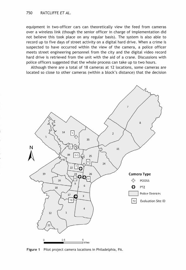
Two areas were designated around each camera site. The first area wasdesignated the target area—the area where the cameras are expected to have apositive effect. Buffer areas were also generated around camera locations.These areas were designed to be likely places in the surrounding neighborhoodof the cameras where crime activity could potentially be displaced. The bufferarea is also a zone where potential diffusion of benefits (Clarke & Weisburd,1994) could occur. This can happen when the cameras exert a benefit tosurrounding areas beyond their target area, and may occur because offendersmove out of the general area of the camera, or offenders at unviewed areascurtail their activity because they think the camera can still see them. Displace-ment areas began as simple 500 ft buffers surrounding the target areas. 500 ftwas chosen as a rounded median estimation of the length of one city block.These 500 ft buffers were then adjusted to account for local geography and roadpatterns surrounding each location. This means that at some locations thedisplacement buffer was slightly less than 500 ft while in others it was greater.While it may seem intuitively better to have uniform displacement areas, doingso ignores the substantial variability in the geography surrounding cameraimplementation areas. For example, the use of actual camera viewsheds canmean that a 500 ft buffer stretches to just short of a neighboring intersection.In circumstances like this, the addition of an extra 20 ft is sufficient to includethe street intersection (and thus the crime at that location) and create a bufferthat is a more realistic approximation of the likely displacement area. Themethod utilized here, while requiring more effort and a greater understandingof local geographic conditions, produces more realistic target and displacementareas. Figure 2 illustrates the unique shape of PTZ buffers compared to themore traditional buffer approach that was utilized for the PODSS cameras.Figure 2 Example of PTZ and PODSS camera target and displacement area. The camera location is shown as a small cross in the center of each image, while the lighter (hash-marked) area near the center is the designated target area. Potential buffer areas (to assess displacement or diffusion of benefits) are shown as dark grey. Individual lines indicate a road network.Finally, as a control on general trends in the surrounding areas beyond thetarget and buffer area, the surrounding police district(s) beyond the displace-ment areas became designated as a control area. As such, the control areas arecomparable across both socio-economic and organizational parameters. First,the control areas represented territory that was within the region of the target(experimental) area, so remained within the generalized socio-economic struc-ture of the block of neighborhoods that make up the police district. By beingwithin the same police district as the cameras, the control areas were alsosusceptible to the same organizational forces that affected the camera areas.Researchers using control areas that are in entirely different police districts runthe risk that the districts without cameras may conduct a different style of



policing or introduce their own crime fighting initiatives that could confoundthe study. Using control areas that are in the same district as the camerasmeans that both target and control areas are policed in generally the samemanner, resulting in greater comparability of area for the study.

Where a camera target or buffer area intersected more than one policedistrict, we used the remainder (all areas not included with target and bufferareas) of the intersecting police districts combined. Table 1 provides details ofhow these control areas were constructed, along with the number of months thecameras had been operational at the site at the time of evaluation, the specificdates of the pre-/post-camera implementation evaluation period, the cameratype, the number of cameras deployed at that location, and the police district.As can be seen from the last column of the table, the definition of control areaswas confounded by camera sites being relatively close to each other, and some-times on the boundary between police districts.

Crime data

Crime data from January 2005 through August 2007 (32 months) was sourcedfrom the PPD’s Crime Analysis and Mapping Unit. This dataset contained infor-mation about crime type, date, and the x-y coordinates of the crime location,as geocoded by the PPD to a successful geocoding hit rate in excess of 97%; asatisfactory level in excess of minimum geocoding levels estimated throughsimulation processes (Ratcliffe, 2004).

This evaluation limits crimes examined in the study to those that could beexpected to be influenced by CCTV cameras. Therefore, only crimes that gener-ally occur on the street were included in the analysis. In other words, theft froma vehicle is included while theft by shoplifting (because it would happen inside astore away from the view of the camera) is not. The crimes are aggregated into

Figure 2 Example of PTZ and PODSS camera target and displacement area. Thecamera location is shown as a small cross in the center of each image, while the light-er (hash-marked) area near the center is the designated target area. Potentialbuffer areas (to assess displacement or diffusion of benefits) are shown as dark grey.Individual lines indicate a road network.



Tabl

e 1

Spec

ific

atio

n of

wei

ghte

d di

spla

cem

ent

quot

ient

par

amet

ers

Site

Mon

ths

cam

era

oper

atio

nal

Pre-

impl

emen

tati

on

date

s

Post

-im

plem

enta

tion

da

tes

Cam

era

type

No.

of

cam

eras

Loca

tion

(p

olic

e di

stri

ct)

Cont

rol a

rea

com

posi

tion

19

Jan

2005

–Nov

20

06D

ec 2

006–

Aug

2007

POD

SS1

1414

th p

olic

e di

stri

ct c

rim

e to

tals

, m

inus

tar

get

and

disp

lace

men

t ar

eas

for

cam

era

at s

ite

12

9Ja

n 20

05–N

ov

2006

Dec

200

6–Au

g 20

07PO

DSS

239

39th

pol

ice

dist

rict

cri

me

tota

ls,

min

us t

arge

t an

d di

spla

cem

ent

area

s fo

r ca

mer

as a

t si

te 2

3–5

10Ja

n 20

05–O

ct

2006

Nov

200

6–Au

g 20

07PO

DSS

425

25th

and

39t

h po

lice

dist

rict

cri

me

tota

ls,

min

us

targ

et a

nd d

ispl

acem

ent

area

s fo

r ca

mer

as a

t si

tes

2–5

610

Jan

2005

–Oct

20

06N

ov 2

006–

Aug

2007

POD

SS1

2522

nd,

25th

and

26t

h po

lice

dist

rict

cri

me

tota

ls,

min

us t

arge

t an

d di

spla

cem

ent

area

s fo

r ca

mer

as a

t si

tes

3, 4

, 5,

6,

7, a

nd 9

711

Jan

2005

–Sep

20

06O

ct 2

006–

Aug

2007

PTZ

222

22nd

pol

ice

dist

rict

cri

me

tota

ls,

min

us t

arge

t an

d di

spla

cem

ent

area

s fo

r ca

mer

as a

t si

te 2

811

Jan

2005

–Sep

20

06O

ct 2

006–

Aug

2007

PTZ

223

6th,

9th

and

23r

d po

lice

dist

rict

cri

me

tota

ls,

min

us t

arge

t an

d di

spla

cem

ent

area

s fo

r ca

mer

as a

t si

te 8

914

Jan

2005

–Jun

20

06Ju

ly 2

006–

Aug

2007

PTZ

226

26th

pol

ice

dist

rict

cri

me

tota

ls,

min

us t

arge

t an

d di

spla

cem

ent

area

s fo

r ca

mer

a at

sit

e 9

1011

Jan

2005

–Sep

20

06O

ct 2

006–

Aug

2007

PTZ

417

17th

pol

ice

dist

rict

cri

me

tota

ls,

min

us t

arge

t an

d di

spla

cem

ent

area

s fo

r ca

mer

a at

sit

e 10



three categories; serious crime (UCR Part 1 street offenses), disorder crime(UCR Part 2 street offenses), and all crime (the sum of the unweighted seriousand disorder crime categories). The full list of crimes included in the analysiscan be found in Appendix A.

Analysis

Two methods were utilized to investigate the impact of camera implementationupon localized crime. HLM allows for rigorous statistical evaluation of cameraimplementation while controlling for factors such as seasonality and ongoingtrends. The use of HLM in this analysis, however, is limited because it is notpossible to investigate specific cameras or specific locations. In order to furtherinvestigate the effects of specific cameras we utilize WDQ as described byBowers and Johnson (2003). We discuss the HLM model first.

Hierarchical Linear Modeling

HLM is a type of statistical analysis that recognizes nested data structures(Raudenbush & Bryk, 2002; Snijders & Bosker, 1999). This also applies torepeated observations across individuals or locations (Laird & Ware, 1982). Thecurrent analysis examines time nested within camera locations. The particularanalysis completed has a number of practical benefits. First, it includes a vari-able that statistically controls for seasonal effects on crime. Seasonal effectscould be particularly important for the street crimes under analysis here,because people spend more time outside when the weather is warmer. Secondly,the analysis controls for preexisting temporal trends at each camera location.Failing to control for these pre-camera implementation trends could result inunder or overestimating the cameras’ effects on crime patterns. Examples ofsuch pre-camera implementation trends include the possibility of regenerationtaking place near a camera location potentially resulting in a generally decliningcrime trend—an additional effect beyond simple seasonal variation.

Specific HLM variables are as follows. The length of month variable repre-sents the number of days per month, given that it is reasonable to expect thatlonger months will have higher crime counts. The temporal trend variablerepresents the sequential position of the month in the data series in the level-1HLM equation. This variable captures the linear trend of crime around thecameras over time at each location. This variable can be positive if crime isgenerally increasing, negative if crime is decreasing or zero if the crime trend isshowing no change over time. The ongoing effects of changes over time aretailored for each location in that each camera location is allowed to have itsown unique linear crime trend over time.

A seasonal effect variable controls for seasonality through the use of a valueto represent the monthly average of the average daily temperature. These



figures were obtained from the historical archives provided by WeatherUnderground (available at www.wunderground.com/history). The camera vari-able represents the effects of camera implementation (0 = non-camera month;1 = camera implemented). Because of the other variables included, this variablerepresents camera implementation while controlling for length of the month,pre-existing crime trends, and seasonal effects.

At level-1, the units are repeated measurements (monthly observations fromJanuary 2005 through August 2007) on the dependent (crime count) and inde-pendent (camera implementation, length of month, pre-existing crime trends,and seasonal effects) variables. These level-1 repeated measures are nestedwithin the level-2 units (cameras). In this analysis, three dependent variablesare utilized; serious crimes, disorder crimes, and all crime (the sum of bothserious offenses and disorder crimes).

These separate dependent variables were modeled using the same specifica-tions for the independent variables. All three dependent variables are non-normally distributed. For this reason, the HLM models are specified as a Poissondistribution with over-dispersion.2 Thus, all models follow the specification:

Where Crime Countit is the number of crimes occurring within the camerabuffer area for camera i at time t; β0i is the mean crime count in camera i inApril 2006 (the mid-point of the study period) when length of month andseasonal effects are set to their mean for camera i; β1i is the slope coefficientfor length of month for camera i; β2i is the slope for the linear temporal trendsat camera i; β3i is the slope coefficient for the impact of seasonal trends atcamera i; β4i is the slope coefficient for the dummy variable representingcamera implementation at camera location i; and rit is the residual or unex-plained variance.

The level-2 model was specified as:

where γ00 is the average intercept (mean crime count) in April 2006 across allcameras; γ10 represents the fixed slope of the length of the month; γ20 repre-

2. All three dependent variables demonstrate over-dispersion with a standard deviation greaterthan the mean: serious crime m = 3.86, sd = 4.48; disorder crime m = 15.60, sd = 18.22; allcrime m = 19.46, sd = 21.51.

Crime Count Length of month Temporal trend

Seasonal effect Camera rit i i i

i i it

= + ++ + +

β β ββ β

0 1 2

3 4

( ) ( )

( ) ( )

β γβ γβ γβ γβ γ

0 00 0

1 10

2 20 2

3 30

4 40

i i

i

i i

i

i

u

u

= +== +==



sents the varying slope of ongoing temporal trends; γ30 represents the fixedslope of seasonal effects; γ40 represents the fixed slope of camera implementa-tion; and u0i and u2i are the residuals or unexplained between camera variancein the intercept and temporal trend slope coefficients, respectively.

Weighted Displacement Quotient (WDQ)

Bowers and Johnson’s (2003) WDQ is employed to determine if differencesbetween the target and buffer areas are a result of displacement from thetarget area or a diffusion of benefits from the use of CCTV surveillance in thetarget area. The determination of a WDQ first requires the researcher to deter-mine three operational areas; the target area where the crime reduction strat-egy has been deployed (in this case, CCTV camera viewsheds), a buffer areathat is estimated to be the most likely location that crime would be displacedto, and a control area that acts as a check on general crime trends that areaffecting the region in general. The equation for the WDQ is as follows:

where A is the count of crime events in the target area, B is the count ofcrime events in the buffer area, C is the count of crime events in the controlarea, t1 is the time since the camera(s) have been active, and t0 is the pre-intervention time period (in this case, an equivalent number of monthsimmediately prior to the installation of the cameras). The examination of thedifference between the buffer and control areas from the pre-intervention tothe intervention period provides the measure of displacement or diffusion intothe buffer area, while the differences between the target and control arearatios at both times provide the measure of success for the intervention. Theequation above is therefore comprised of both a buffer displacement measure(Bt1/Ct1 – Bt0/Ct0) and a success measure (At1/Ct1 – At0/Ct0).

If the success measure is a positive value, this indicates that the cameraimplementation was not successful in reducing crime when compared to thecontrol area. In this situation—indicating the camera implementation was unsuc-cessful in reducing crime—then neither the displacement measure nor the WDQvalues are calculated. Only if the success measure indicates a reduction in crimein the target area is a displacement measure calculated. If the displacementmeasure is a positive number, this indicates that when the cameras were imple-mented, crime went up in the buffer area to a greater extent than in the controlarea. This is suggestive of a displacement effect. A negative displacement valuesuggests a diffusion of benefits from the target area to the buffer area.

Finally, these two values are combined to form the WDQ value. According toBowers and Johnson (2003), WDQ values greater than 1 indicate crime reduc-tions in the target area and substantial diffusion of benefits to the surrounding

WDQ (B C B C A C A C= − −t t t t t t t t1 1 0 0 1 1 0 0/ / )/( / / ),



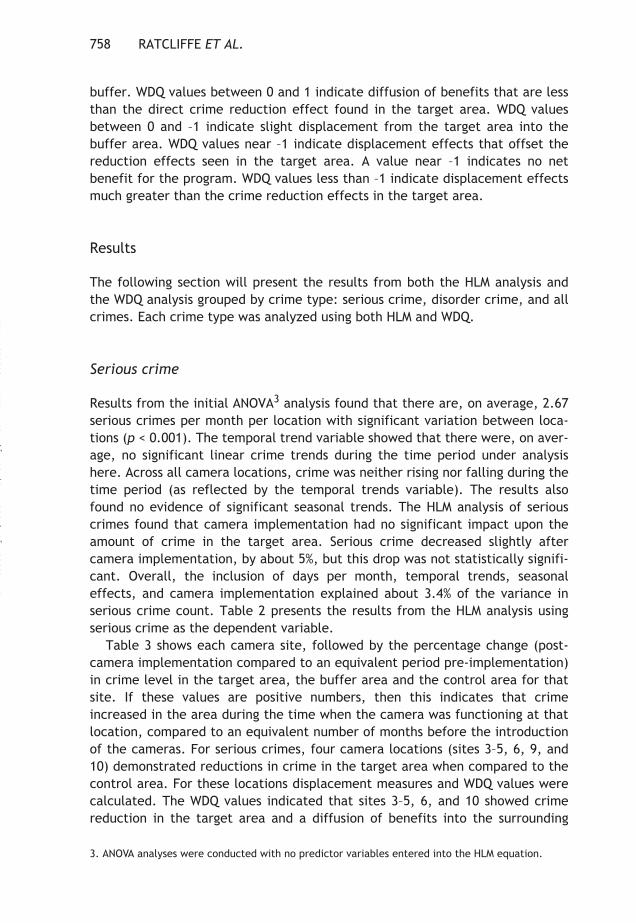
buffer. WDQ values between 0 and 1 indicate diffusion of benefits that are lessthan the direct crime reduction effect found in the target area. WDQ valuesbetween 0 and –1 indicate slight displacement from the target area into thebuffer area. WDQ values near –1 indicate displacement effects that offset thereduction effects seen in the target area. A value near –1 indicates no netbenefit for the program. WDQ values less than –1 indicate displacement effectsmuch greater than the crime reduction effects in the target area.

Results

The following section will present the results from both the HLM analysis andthe WDQ analysis grouped by crime type: serious crime, disorder crime, and allcrimes. Each crime type was analyzed using both HLM and WDQ.

Serious crime

Results from the initial ANOVA3 analysis found that there are, on average, 2.67serious crimes per month per location with significant variation between loca-tions (p < 0.001). The temporal trend variable showed that there were, on aver-age, no significant linear crime trends during the time period under analysishere. Across all camera locations, crime was neither rising nor falling during thetime period (as reflected by the temporal trends variable). The results alsofound no evidence of significant seasonal trends. The HLM analysis of seriouscrimes found that camera implementation had no significant impact upon theamount of crime in the target area. Serious crime decreased slightly aftercamera implementation, by about 5%, but this drop was not statistically signifi-cant. Overall, the inclusion of days per month, temporal trends, seasonaleffects, and camera implementation explained about 3.4% of the variance inserious crime count. Table 2 presents the results from the HLM analysis usingserious crime as the dependent variable.

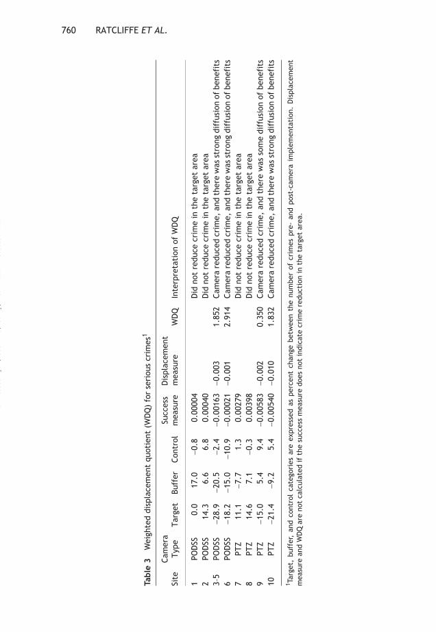
Table 3 shows each camera site, followed by the percentage change (post-camera implementation compared to an equivalent period pre-implementation)in crime level in the target area, the buffer area and the control area for thatsite. If these values are positive numbers, then this indicates that crimeincreased in the area during the time when the camera was functioning at thatlocation, compared to an equivalent number of months before the introductionof the cameras. For serious crimes, four camera locations (sites 3–5, 6, 9, and10) demonstrated reductions in crime in the target area when compared to thecontrol area. For these locations displacement measures and WDQ values werecalculated. The WDQ values indicated that sites 3–5, 6, and 10 showed crimereduction in the target area and a diffusion of benefits into the surrounding

3. ANOVA analyses were conducted with no predictor variables entered into the HLM equation.



buffer area. Site 9 shows crime reduction in the target area and more modestcrime reduction in the surrounding buffer area. Table 3 presents the results ofthe WDQ analysis for serious crime.

Disorder crime

Results from the ANOVA analysis finds that there are, on average, 8.34 disordercrimes per month per location with significant variation between locations(p < 0.001). Table 4 provides the results of the HLM analysis when investigatingthe impact of cameras upon disorder crimes. As expected the length of monthwas a significant predictor of higher crime counts. The temporal trend variableshowed that the number of disorder crimes increased slightly during the studyperiod, on average, across all locations. The expected count of disorder crimesincreased, on average, about 1.3% every month across the evaluation sites. Thesignificance of the seasonality variable indicates that there are more disordercrimes in warmer months. The coefficient for the camera variable indicatesthat camera implementation significantly reduced disorder crime in the targetarea. After camera implementation, the average expected disorder crime countfor the target areas was 16% lower, after controlling for all other variables.Overall, the inclusion of days per month, temporal trends, seasonal effects, andcamera implementation explained about 10.4% of the variance in disorder crimecount.

Table 2 HLM results for serious crime1

Fixed Effects Coefficient (S.E.) Event rate ratio Confidence interval

Number of days per month

0.064(0.034)

1.066 0.997–1.140

Temporal trend 0.002(0.006)

1.002 0.989–1.015

Seasonality 0.003(0.002)

1.003 1.000–1.007

Camera −0.050(0.104)

0.951 0.774–1.169

Random effect Variance component Chi-square DfBetween camera (level-2)

Mean crime count 0.859** 1855.120 9Temporal trend 0.007* 17.394 9

Within-camera (level-1)Residual variation 0.889

Total variance explained 3.357%

*p < 0.05, **p < 0.001.1Dependent variable specified as Poisson distribution with over-dispersion. Number of days permonth, seasonality, and camera implementation dummy were specified as fixed slopes. Thetemporal trend variable was specified as varying slope.



Tabl

e 3

Wei

ghte

d di

spla

cem

ent

quot

ient

(W

DQ

) fo

r se

riou

s cr

imes

1

Site

Cam

era

Type

Targ

etBu

ffer

Cont

rol

Succ

ess

mea

sure

Dis

plac

emen

t m

easu

reW

DQ

Inte

rpre

tati

on o

f W

DQ

1PO

DSS

0.0

17.0

−0.8

0.00

004

Did

not

red

uce

crim

e in

the

tar

get

area

2PO

DSS

14.3

6.6

6.8

0.00

040

Did

not

red

uce

crim

e in

the

tar

get

area

3–5

POD

SS−2

8.9

−20.

5−2

.4−0

.001

63−0

.003

1.85

2Ca

mer

a re

duce

d cr

ime,

and

the

re w

as s

tron

g di

ffus

ion

of b

enef

its

6PO

DSS

−18.

2−1

5.0

−10.

9−0

.000

21−0

.001

2.91

4Ca

mer

a re

duce

d cr

ime,

and

the

re w

as s

tron

g di

ffus

ion

of b

enef

its

7PT

Z11

.1−7

.71.

30.

0027

9D

id n

ot r

educ

e cr

ime

in t

he t

arge

t ar

ea8

PTZ

14.6

7.1

−0.3

0.00

398

Did

not

red

uce

crim

e in

the

tar

get

area

9PT

Z−1

5.0

5.4

9.4

−0.0

0583

−0.0

020.

350

Cam

era

redu

ced

crim

e, a

nd t

here

was

som

e di

ffus

ion

of b

enef

its

10PT

Z−2

1.4

−9.2

5.4

−0.0

0540

−0.0

101.

832

Cam

era

redu

ced

crim

e, a

nd t

here

was

str

ong

diff

usio

n of

ben

efit

s

1 Tar

get,

buf

fer,

and

con

trol

cat

egor

ies

are

expr

esse

d as

per

cent

cha

nge

betw

een

the

num

ber

of c

rim

es p

re-

and

post

-cam

era

impl

emen

tati

on.

Dis

plac

emen

tm

easu

re a

nd W

DQ

are

not

cal

cula

ted

if t

he s

ucce

ss m

easu

re d

oes

not

indi

cate

cri

me

redu

ctio

n in

the

tar

get

area

.



WDQs were calculated using disorder crimes as the outcome variable. Sites 3–5, 8, 9, and 10 had success measures indicating a reduction in crime after theimplementation of the cameras; therefore, displacement measures werecalculated for these locations. For these four sites, only one had a negativedisplacement measure. Overall, sites 1, 2, 6, and 7 had no reduction in crimeafter implementation of the cameras. Sites 3–5 and 10 had reductions in thetarget area but these reductions were offset by displacement into the surround-ing areas. Site 8 had a reduction in crime in the target area but slight increasesin the buffer area, though there was an overall reduction in crime. Only camera9 demonstrated a crime reduction in the target area with a diffusion of benefitinto the buffer area. Table 5 presents the findings from the WDQ analysis fordisorder crimes.

All Crime

The final analysis combined serious crime with disorder events. This had theeffect of weighting each incident equally, and is reported here as a measure ofthe value of CCTV cameras for all incidents, irrespective of seriousness. Table 6provides the results of the HLM analysis when utilizing all (both serious anddisorder) crime. Results from the ANOVA analysis find that there are, on aver-age, 11.35 crimes per month per location with significant variation betweenlocations (p < 0.001). The temporal trend variable was not significant; there wasno change in trend during the study period. The length of month variable wassignificant with each additional day being related to a 5% increase in theexpected count per camera. Crime counts were also significantly higher duringmonths with higher temperatures. The implementation of cameras significantly

Table 4 HLM results for disorder crime1

Fixed effects Coefficient (S.E.) Event rate ratio Confidence interval

Number of days per month 0.052* (0.023) 1.054 1.007–1.103Temporal trend 0.013* (0.006) 1.013 1.001–1.026Seasonality 0.006** (0.070) 1.006 1.004–1.009Camera −0.174* (0.001) 0.840 0.733–0.963


Mean crime count 1.578** 6357.731 9Temporal trend 0.000** 68.442 9

Within-camera (level-1)Residual variation 0.1627

Total variance explained 10.421%

*p < 0.05, **p < 0.001.1Dependent variable specified as Poisson distribution with over-dispersion. Number of days permonth, seasonality, and camera implementation dummy were specified as fixed slopes. Thetemporal trend variable was specified as varying slope.



Tabl

e 5

Wei

ghte

d di

spla

cem

ent

quot

ient

(W

DQ

) fo

r di

sord

er c

rim

es1

Site

Cam

era

type

Targ

etBu

ffer

Cont

rol

Succ

ess

mea

sure

Dis

plac

emen

t m

easu

reW

DQ

Inte

rpre

tati

on o

f W

DQ

1PO

DSS

19.2

−20.

2−9

.80.

0023

Did

not

red

uce

crim

e in

the

tar

get

area

2PO

DSS

11.8

−8.8

−6.7

0.00

17D

id n

ot r

educ

e cr

ime

in t

he t

arge

t ar

ea3–

5PO

DSS

−1.1

9.4

3.8

−0.0

002

0.00

1−3

.454

Cam

era

redu

ced

crim

e, b

ut d

ispl

acem

ent

nega

ted

gain

s6

POD

SS−3

.0−2

6.5

−16.

70.

0003

Did

not

red

uce

crim

e in

the

tar

get

area

7PT

Z0.

90.

0−4

.10.

0008

Did

not

red

uce

crim

e in

the

tar

get

area

8PT

Z−1

6.4

10.9

5.4

−0.0

072

0.00

1−0

.209

Cam

era

redu

ced

crim

e, b

ut t

here

was

slig

ht d

ispl

acem

ent

(net

gai

n)9

PTZ

−35.

9−2

1.9

−6.7

−0.0

107

−0.0

050.

479

Cam

era

redu

ced

crim

e, a

nd t

here

was

som

e di

ffus

ion

of b

enef

its

10PT

Z−2

.721

.08.

1−0

.004

00.

009

−2.2

67Ca

mer

a re

duce

d cr

ime,

but

dis

plac

emen

t ne

gate

d ga

ins

1 Tar

get,

buf

fer,

and

con

trol

cat

egor

ies

are

expr

esse

d as

per

cent

cha

nge

betw

een

the

num

ber

of c

rim

es p

re-

and

post

-cam

era

impl

emen

tati

on.

Dis

plac

emen

tm

easu

re a

nd W

DQ

are

not

cal

cula

ted

if t

he s

ucce

ss m

easu

re d

oes

not

indi

cate

cri

me

redu

ctio

n in

the

tar

get

area

.



reduced the number of crime events within the target areas. The monthsfollowing the implementation of the cameras saw a statistically significant13.3% reduction in expected crime counts after controlling for the other factors(p < 0.05). Overall, the inclusion of days per month, temporal trends, seasonaleffects, and camera implementation explained about 12.9% of the variance inthe crime count.

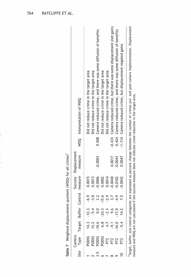
WDQ values were calculated for all crimes. Camera locations 3–5, 8, 9, and10 demonstrated crime reductions in the target area after implementation ofthe cameras. Sites 3–5 and 9 saw some diffusion of benefits into the surroundingbuffer area. Site 8 saw a slight displacement of crime into the buffer area,though the crime reduction in the target area was enough to offset theeffects of displacement. Finally, at site 10, the reduction of crime in the targetarea was offset by the displacement of crime into the surrounding buffer area.Table 7 reports the results from the WDQ analysis on all crimes.

Discussion

Overall, results from the HLM analysis suggest that the introduction of thecameras was associated with a 13% reduction in all crime in the target areassurrounding CCTV implementation sites. The reduction was statisticallysignificant, after controlling for general temporal trends at each camera site,seasonality, and the number of days in each month. This reduction was largely

Table 6 HLM results for all crime1

Fixed effects Coefficient (S.E.) Event rate ratio Confidence interval

Number of days per month 0.055*(0.020)

1.056 1.014–1.099

Temporal trend 0.010(0.005)

1.010 0.999–1.020

Seasonality 0.006**(0.001)

1.006 1.003–1.008

Camera −0.142*(0.061)

0.867 0.768–0.979


Mean crime count 1.292** 6843.160 9Temporal trend 0.000** 49.689 9

Within-camera (level-1)Residual variation 1.590Total variance explained 12.855%

*p< 0.05, **p < 0.001.1Dependent variable specified as Poisson distribution with over-dispersion. Number of days permonth, seasonality, and camera implementation dummy were specified as fixed slopes. Thetemporal trend variable was specified as varying slope.



Tabl

e 7

Wei

ghte

d di

spla

cem

ent

quot

ient

(W

DQ

) fo

r al

l cri

mes

1

Site

Cam

era

Type

Targ

etBu

ffer

Cont

rol

Succ

ess

mea

sure

Dis

plac

emen

t m

easu

reW

DQ

Inte

rpre

tati

on o

f W

DQ

1PO

DSS

14.3

−12.

3−6

.90.

0015

Did

not

red

uce

crim

e in

the

tar

get

area

2PO

DSS

12.2

−5.4

−3.8

0.00

13D

id n

ot r

educ

e cr

ime

in t

he t

arge

t ar

ea3–

5PO

DSS

−10.

60.

02.

2−0

.000

6−0

.000

30.

508

Cam

era

redu

ced

crim

e, a

nd t

here

was

som

e di

ffus

ion

of b

enef

its

6PO

DSS

−6.8

−24.

3−1

5.6

0.00

02D

id n

ot r

educ

e cr

ime

in t

he t

arge

t ar

ea7

PTZ

4.7

−2.3

−2.9

0.00

14D

id n

ot r

educ

e cr

ime

in t

he t

arge

t ar

ea8

PTZ

−9.1

9.6

3.7

−0.0

040

0.00

17−0

.433

Cam

era

redu

ced

crim

e, b

ut t

here

was

som

e di

spla

cem

ent

(net

gai

n)9

PTZ

−34.

0−1

7.0

−4.9

−0.0

102

−0.0

043

0.42

4Ca

mer

a re

duce

d cr

ime,

and

the

re w

as s

ome

diff

usio

n of

ben

efit

s10

PTZ

−5.4

14.2

7.5

−0.0

042

0.00

47−1

.114

Cam

era

redu

ced

crim

e, b

ut d

ispl

acem

ent

nega

ted

gain

s

1 Tar

get,

buf

fer,

and

con

trol

cat

egor

ies

are

expr

esse

d as

per

cent

cha

nge

betw

een

the

num

ber

of c

rim

es p

re-

and

post

-cam

era

impl

emen

tati

on.

Dis

plac

emen

tm

easu

re a

nd W

DQ

are

not

cal

cula

ted

if t

he s

ucce

ss m

easu

re d

oes

not

indi

cate

cri

me

redu

ctio

n in

the

tar

get

area

.



due to a decline in disorder offenses, as the frequency of serious crimes aroundeach camera location was generally too low to detect a measurable impact inserious crime alone.

This does not mean that serious crime was not impacted. It is worth notingthat one would normally expect seasonality and the length of month to be signif-icant in an analysis of serious street crime. Because the coefficients for thesevariables were not statistically significant, this suggests that a possible cause forthis lack-of-finding is that in each month there were insufficient crimes in thetarget area for the technique to detect a statistically significant change. Forexample, serious crime in the target area for site 1 was two per month prior toand after camera installation. The values for the target area of site 2 were evenlower. With this in mind, the lack of statistical significance in the serious crimecategory could probably be better interpreted as resulting from a lack ofreported serious crime generally, rather than a failure of the CCTV initiative. Inthe same vein, Mazerolle et al. (2002) could not attempt an evaluation of violentcrimes around CCTV locations because of the low base rate in the target areas.

A further cause of the low number of serious offenses within the purview ofeach camera may be the manner in which the dependent variable wasconstructed. First, rather than including a broad measure of all serious crime(e.g., Squires, 2003), only those serious offenses that the CCTV cameras wereexpected to influence were included in the dependent variable count. Secondly,rather than setting an arbitrary buffer distance out from each camera location,individual viewsheds were examined for the PTZ cameras. Had we taken theapproach of Sarno, Hough, and Bulos (1999) and established a fixed buffer of200 meters (just over 650 feet), we would most likely have included a numberof offenses that occurred out of the view of a camera.

The introduction of CCTV was associated with considerably different impactson crime at each site. At half of the sites, crime did not reduce in the targetarea. At four sites, serious crime was reduced and there was evidence of adiffusion of positive benefits to surrounding streets. At some sites, crime wasreduced in the target area but there was apparent displacement to surroundingstreets. Therefore the 13% reduction in overall crime was comprised of verydifferent behaviors at CCTV evaluation sites.

The results of the WDQ are further complicated by the differences seenacross camera type. Both PTZ cameras and PODSS cameras have examples ofsuccessful crime reduction in their target areas. From a policy perspectivechoosing between PTZ cameras and PODSS cameras can be important. Thesecameras differ on both their usefulness to police investigations and their initialinstallation and ongoing maintenance cost. However, from an outcome perspec-tive, it may be that the actual camera mechanism may be less important thanthe choice of location. This might help to explain why both camera typesappeared to have successes and failures. It may have been the location selectedfor camera implementation, not the camera type, that ultimately determinedthe crime suppression effects. Of course, this is merely raised as a hypotheticalexplanation given the limited number of cameras and sites under examination in



this study. It is certainly a finding from the study that merits further investiga-tion with a larger study.

Inevitably in a study of this nature there are some limitations. Data weregenerously provided by the police department of the City of Philadelphia, andwere provided already geocoded and with most address-specific informationremoved (beyond the location coordinates). As such, ground-truthing theaccuracy of the geocoding process employed by the city was not possible. Ourextensive previous experience with PPD data, as well as personal contact withthe GIS Mapping Unit, lead us to have confidence in the accuracy and precisionof their geocoding processes such that we could attempt this study, however, itshould be noted that we did not perform the geocoding ourselves.

Perhaps the biggest limitation of the HLM analysis is its inability to disaggre-gate the effectiveness of each camera type. An attempt to control for the typeof camera at each location is met with difficulty primarily because there are sofew cameras to analyze. Disaggregating the analysis by the type of cameraleaves too few cases for a robust statistical analysis. This line of inquiry,however, is a worthy area of further investigation. From a practical perspective,PTZ cameras and PODSS cameras have substantial differences in both initial andongoing monitoring cost. Therefore, in order to better understand the effects ofdifferent cameras at different locations, a WDQ analysis was utilized.

Unlike the HLM analysis, WDQ is not able to incorporate sensitivity to season-ality patterns or to control for subtle trends in changing crime patterns overtime. It compensates for this by incorporating a control area measurement,used to adjust the result for differences in an area not related to the target ordisplacement zones of the cameras. In other words, the control area provides anindication of what was happening in unaffected areas, and is a broad indicationof trends over the same period of time as the CCTV intervention. WDQ does,however, provide the opportunity to measure a general indication of the successof each evaluation site, something not possible with the HLM analysis.

Policy-makers looking to this study to provide a definitive answer are likely tobe a little disappointed in the ambiguity of the results. The reduction in overallcrime of 13% is welcome, though the WDQ results that suggest some camerasites were unsuccessful in reducing crime at their locations casts a cloud overany suggestion of there being a benefit to blanket citywide CCTV coverage. Thefinding does fit into the broad pattern of results typified by the multi-sitestudy by Gill and Spriggs (2005), the meta-analysis of Welsh and Farrington(2007, p. 46) who found a ‘small but significant desirable effect on crime,’ andthe review by Ratcliffe (2006, p. 19) that found ‘achieving statisticallysignificant reductions in crime can be difficult.’

Evaluating the effectiveness of CCTV is often confounded by the conduct ofother crime prevention initiatives at the same time, making it difficult to teaseout the benefit of the cameras alone; however, some reviews have noted thebenefit of bundling CCTV with other crime prevention programs as a package ofmeasures. This may help to overcome the public perception that CCTV is a‘silver bullet’ that will reduce crime in the absence of any other socio-economic



or opportunity-related changes to the local environment. Farrington, Gill,Waples, & Argomaniz (2007) concluded that CCTV could reduce crime in carparks, but was generally ineffective in residential areas or city centers; theyalso suggested that the benefits of CCTV may increase when implementedalongside improved lighting.

Camera success as an investigative tool (an additional factor beyond crimereduction worth considering, according to Gill & Spriggs, 2005) is potentiallytied to factors such as operator familiarity with the area under examination, thelikely offenders in an area, the nature of businesses and individuals in a cameralocation, and the type of crime common to the camera area. Further potentialfactors can also include the ability of local police to have sufficient resources torespond quickly to any incident viewed on the camera, as well as the nature ofthe local geography at a camera location; even the quickest police work can behampered by easy and accessible escape routes for offenders. Future studies ofcamera effectiveness might care to consider these factors as controls on cameraefficiency in the crime prevention arena.

Finally, we did not examine the issue of public perceptions of safety. It maybe that CCTV is politically palatable if public surveys and interviews indicatedimprovements in perception of safety and quality of life within the range ofCCTV even in the face of a lack of crime reduction benefits. The evidence fromthe British studies is not optimistic (see Gill & Spriggs, 2005); however, it shouldbe considered an avenue for further work in the evaluation of CCTV in the USA.

Conclusion

This evaluation finds that when serious and disorder offenses were consideredtogether crime was reduced by 13% after the implementation of the CCTVcameras while controlling for length of month, seasonal effects, and the uniquetemporal trends at each camera. WDQs were then utilized in an attempt todisaggregate this finding by location and camera type. While there was evidencethat camera implementation had positive effects, the fact that crime did notreduce in the surveillance areas of half the sites examined cannot be ignored.Given the low volume of serious crime at each site (as measured on a monthlybasis), it may be prudent to prioritize future CCTV sites based on an objectivemeasure of the volume of crime at each intersection. Furthermore, given thatthe PTZ cameras are able to view activity at more than one street intersection,selection of future sites would be improved by attempting to find clusters ofstreet intersections and blocks that have crime problems rather than singlecorners. If multiple locations can be viewed effectively from a single camera,this may be a more cost beneficial use of CCTV technology. Finally, the paucityof CCTV evaluations is a hindrance in advancing our understanding of any crimeprevention benefits of surveillance technology, a gap in the research literaturethat criminologists should seek to remedy as soon as possible. Research or not,cities are moving ahead with CCTV systems, and if criminologists are to remain



relevant in this crime prevention expansion, more experimental or high qualityquasi-experimental research is necessary.

Acknowledgments

The researchers would like to thank Commissioner Charles Ramsey and DeputyCommissioner Jack Gaittens, Philadelphia Police Department, for supportingthis project and provision of the necessary data. The views expressed herein arethose of the authors and do not necessarily reflect the views or opinions ofTemple University, the City of Philadelphia, or the Philadelphia PoliceDepartment.

References

Bowers, K. J., & Johnson, S. D. (2003). Measuring the geographical displacement anddiffusion of benefit effects of crime prevention activity. Journal of QuantitativeCriminology, 19(3), 275–301.

Brown, B. (1995). CCTV in town centres: Three case studies (Crime Detection andPrevention Series, Paper 68). London: Home Office.

Bulwa, D. (2008, February 7). New criminal justice chief wants cops monitoring cameras.The San Francisco Chronicle, p. B–3.

Clarke, R. V. (2004). Technology, criminology and crime science. European Journal onCriminal Policy and Research, 10(1), 55–63.

Clarke, R. V., & Felson, M. (1993). Introduction: Criminology, routine activity, and ratio-nal choice. In R. V. Clarke & M. Felson (Eds.), Routine activity and rational choice(Vol. 5, pp. 259–294). New Brunswick, NJ: Transaction.

Clarke, R. V., & Weisburd, D. (1994). Diffusion of crime control benefits. In R. V. Clarke(Ed.), Crime prevention studies (Vol. 2, pp. 165–183). Monsey, NY: Criminal JusticePress.

Cornish, D., & Clarke, R. (1986). The reasoning criminal: Rational choice perspectives onoffending. New York: Springer-Verlag.

Eck, J. (1997). Preventing crime at places. In L. W. Sherman, D. Gottfredson, D. MacKen-zie, J. Eck, P. Reuter, & S. Bushway (Eds.), Preventing crime: What works, whatdoesn’t, what’s promising. Washington DC: National Institute of Justice.

Farrington, D. P., Gill, M., Waples, S. J., & Argomaniz, J. (2007). The effects of closed-circuit television on crime: Meta-analysis of an English national quasi-experimentalmulti-site evaluation. Journal of Experimental Criminology, 3(1), 21–38.

Gill, M., & Spriggs, A. (2005). Assessing the impact of CCTV. London: Research, Develop-ment and Statistics Directorate [Home Office]).

Goldstein, H. (2003). On further developing problem-oriented policing: The most criticalneed, the major impediments, and a proposal. In J. Knutsson (Ed.), Problem-orientedpolicing: From innovation to mainstream (pp. 13–47). Monsey, NY: Criminal JusticePress.

Harada, Y., Yonezato, S., Suzuki, M., Shimada, T., Era, S., & Saito, T. (2004, November17–20,). Examining crime prevention effects of CCTV in Japan. Paper presented at theAmerican Society of Criminology Annual Meeting, Nashville, Tennessee.

Hood, J. (2003). Closed circuit television systems: A failure in risk communication?Journal of Risk Research, 6(3), 233–251.



Jeffery, C. R., & Zahm, D. L. (1993). Crime prevention through environmental design, oppor-tunity theory, and rational choice models. In R. V. Clarke & M. Felson (Eds.), Routineactivity and rational choice (Vol. 5, pp. 323–350). New Brunswick, NJ: Transaction.

Klein, A. (2008, February 21). Cameras have cut violence, study says: Skeptics suspectcrime ‘displacement.’ Washington Post, p. 4.

Laird, N. M., & Ware, J. H. (1982). Random-effects models for longitudinal data. Biomet-rics, 38(4), 963–974.

Mazerolle, L., Hurley, D. C., & Chamlin, M. (2002). Social behavior in public space: Ananalysis of behavioral adaptations to CCTV. Security Journal, 15(1), 59–75.

Ratcliffe, J. H. (2004). Geocoding crime and a first estimate of an acceptable minimumhit rate. International Journal of Geographical Information Science, 18(1), 61–73.

Ratcliffe, J. H. (2006). Video surveillance of public places (Problem-oriented guides forpolice, Response guides series no. 4). Washington DC: Center for Problem OrientedPolicing.

Ratcliffe, J. H. (2008). Intelligence-led policing. Cullompton, Devon: Willan.Raudenbush, S. W., & Bryk, A. S. (2002). Hierarchical linear models: Applications and

data analysis methods. Thousand Oaks, CA: Sage.Sarno, C., Hough, M., & Bulos, M. (1999). Developing a picture of CCTV in Southwark town

centres: Final report. London: Criminal Policy Research Unit, South Bank University.Sivarajasingam, V., Shepherd, J. P., & Matthews, K. (2003). Effect of urban closed circuit

television on assault injury and violence detection. Injury Prevention, 9(4), 312–316.Snijders, T., & Bosker, R. (1999). Multilevel analysis: An introduction to basic and

advanced multilevel modeling. Thousand Oaks, CA: Sage.Squires, P. (2003). An independent evaluation of the installation of CCTV cameras for

crime prevention in the Whitehawk estate, Brighton. Brighton: Health and SocialPolicy Research Centre.

Welsh, B. C., & Farrington, D. P. (2007). Closed-circuit television surveillance and crimeprevention. Stockholm: Swedish National Council for Crime Prevention.

Appendix A

This table lists the offenses examined in this study and their UCR codes. Thecategories are either ‘serious’ (indicating a crime from the FBI UCR Part 1 list)or ‘disorder’ from the (FBI UCR Part 2 list). Both categories are added togetherto create the ‘all crime’ category.

UCR code Crime description Category

111–116 Homicide Serious211, 231 Rape: stranger Serious300–305 Robbery: on the highway Serious306–308 Robbery: purse snatch (force or injury) Serious388–399 Robbery: of vehicle Serious



UCR code Crime description Category

411–416, 421–426, 471–476 Aggravated assault Serious510–517, 520–521, 530–537, 540–541, 591–592

Burglary: residential (including attempts) Serious

550–567, 570–587, 593–594 Burglary: non-residential (including attempts) Serious610, 620, 630 Theft: pocket picking Serious611, 621, 631 Theft: purse snatching Serious614, 618, 624, 628, 634, 638, 640, 641, 642, 643, 649

Theft: from vehicle Serious

720, 722, 724, 726, 728 Vehicle theft (including attempts) Serious710, 721, 723, 727, 730, 741, 743, 725

Recovery of stolen vehicle Serious

801, 802, 813 Simple assault Disorder807, 817 Resisting arrest Disorder1402, 1403, 1404, 1405 Vandalism: public Disorder1406, 1407, 1408, 1409 Vandalism: private Disorder1420, 1421, 1422, 1423 Graffiti Disorder1501–1507, 1516–1518 Violation of the uniform firearms act (VUFA):

adultDisorder

1519 Prohibited offensive weapon: adult Disorder1531–1534, 1541–1544 Violation of the uniform firearms act (VUFA):

juvenileDisorder

1535, 1545 Prohibited offensive weapon: juvenile Disorder1601 Pandering Disorder1602 Solicitation Disorder1708 Public indecency Disorder1710 Statutory sexual assault Disorder1711 Open lewdness Disorder1713 Aggravated indecent assault Disorder1716 Luring Disorder1801–1807 Drug sales Disorder1811–1817 Drug mfg., delivery, or possession with intent

to deliverDisorder

1821–1827 Drug possession Disorder1907 Gambling on highway Disorder2404 Disorderly conduct Disorder2501, 2502 Loitering Disorder3302 Minor disturbance Disorder3306 Disorderly crowd Disorder


the crime reduction effects of public cctv … crime reduction effects of public cctv cameras: a...

Documents