the cusum median chart for known and estimated parameters · pdf filesearchers and...

THE CUSUM MEDIAN CHART FOR KNOWN ANDESTIMATED PARAMETERS

Authors: Philippe Castagliola– Universite de Nantes & LS2N UMR CNRS 6004,

Nantes, France ([email protected])

Fernanda Otilia Figueiredo– Faculdade de Economia da Universidade do Porto & CEAUL,

Porto, Portugal ([email protected])

Petros E. Maravelakis– Department of Business Administration, University of Piraeus,

Piraeus, Greece ([email protected])

Abstract:

• The usual CUSUM chart for the mean (CUSUM-X) is a chart used to quickly detectsmall to moderate shifts in a process. In presence of outliers, this chart is known tobe more robust than other mean-based alternatives like the Shewhart mean chart butit is nevertheless affected by these unusual observations because the mean (X) itselfis affected by the outliers. An outliers robust alternative to the CUSUM-X chartis the CUSUM median (CUSUM-X) chart, because it takes advantage of the robustproperties of the sample median. This chart has already been proposed by otherresearchers and compared with other alternative charts in terms of robustness, but itsperformance has only been investigated through simulations. Therefore, the goal ofthis paper is not to carry out a robustness analysis but to study the effect of parameterestimation in the performance of the chart. We study the performance of the CUSUM-X chart using a Markov chain method for the computation of the distribution and themoments of the run length. Additionally, we examine the case of estimated parametersand we study the performance of the CUSUM-X chart in this case. The run lengthperformance of the CUSUM-X chart with estimated parameters is also studied usinga proper Markov chain technique. Conclusions and recommendations are also given.

Key-Words:

• Average run length; CUSUM chart; Estimated parameters; Median; Order statistics.

AMS Subject Classification:

• 62G30, 62P30.

2 P. Castagliola and F.O. Figueiredo and P. Maravelakis

The CUSUM Median Chart for Known and Estimated Parameters 3

1. INTRODUCTION

A main objective for a product or a process is to continuously improve itsquality. This goal, in statistical terms, may be expressed as variability reduction.Statistical Process Control (SPC) is a well known collection of methods aimingat this purpose and the control charts are considered as the main tools to detectshifts in a process. The most popular control charts are the Shewhart charts,the Cumulative Sum (CUSUM) charts and the Exponentially Weighted MovingAverage (EWMA) charts. Shewhart type charts are used to detect large shifts ina process whereas CUSUM and EWMA charts are known to be fast in detectingsmall to moderate shifts.

The usual Shewhart chart for monitoring the mean of a process is the Xchart. It is very efficient for detecting large shifts in a process (see for exampleTeoh et al., 2014). An alternative chart used for the same purpose is the median(X) chart. The median chart is simpler than the X chart and it can be easilyimplemented by practitioners. The main advantages of the X chart over the Xchart is its robustness against outliers, contamination or small deviations fromnormality. This property is particularly important for processes running for along time. Usually, in such processes, the data are not checked for irregularbehaviour and, therefore, the X chart is an ideal choice.

The CUSUM-X control chart has been introduced by Page (1954). It isable to quickly detect small to moderate shifts in a process. The CUSUM-Xcontrol chart uses information from a long sequence of samples and, therefore,it is able to signal when a persistent special cause exists (see for instance Nenesand Tagaras (2006) or Liu et al. (2014)). However, since it is mean-based, theCUSUM-X suffers from the inefficiency of the mean X to correctly handle out-liers, contamination or small deviations from normality. A natural alternativesolution to overcome this problem is the CUSUM-X chart. This chart has al-ready been proposed by Yang et al. (2010). In their paper they compare itsperformance with the Shewhart, EWMA and CUSUM charts for the mean undersome contaminated normal distributions using only simulation procedures. Thischart has also been considered by Nazir et al. (2013a), again in a simulation studywith other CUSUM charts, in order to compare their performance for the phaseII monitoring of location in terms of robustness against non-normality, specialcauses of variation and outliers.

In the last decades, different types of control charts for variable and countdata based on CUSUM schemes, in univariate or multivariate cases, were pro-posed in the literature. Here we only mention some recent and less traditionalworks on robust and enhanced CUSUM schemes, nonparametric and adaptiveCUSUM control charts and CUSUM charts for count and angular data. Theinterested reader could also take into account the references in the paper thatfollow.


Ou et al. (2011, 2012) carried out a comparative study to evaluate theperformance and robustness of some typical X, CUSUM and SPRT type controlcharts for monitoring either the process mean or both the mean and variance,also providing several design tables to facilitate the implementation of the opti-mal versions of the charts. Nazir et al. (2013b), following the same methodologyused in Nazir et al. (2013a), but for monitoring the dispersion, considered severalCUSUM control charts based on different scale estimators, and analyzed its per-formance and robustness. Qiu and Zhang (2015) investigated the performanceof some CUSUM control charts for transformed data in order to accommodatedeviations from the normality assumption when monitoring the process data, andthey compared its efficiency with alternative nonparametric control charts. Toimprove the overall performance of the CUSUM charts to detect small, mod-erate and large shifts in the process mean, Al-Sabah (2010) and Abujiya et al.(2015) proposed the use of special sampling schemes to collect the data, such asthe ranked set sampling scheme and some extensions of it, instead of using thetraditional simple random sampling. Saniga et al. (2006, 2012) discussed theeconomic advantages of the CUSUM versus Shewhart control charts to monitorthe process mean when one or two components of variance exist in a process.

The use of nonparametric control charts has attracted the attention of re-searchers and practitioners. Chatterjee and Qiu (2009) proposed a nonparametriccumulative sum control chart using a sequence of bootstrap control limits to mon-itor the mean, when the data distribution is non-normal or unknown. Li et al.(2010b) considered nonparametric CUSUM and EWMA control charts based onthe Wilcoxon rank-sum test for detecting mean shifts, and they discussed theeffect of phase I estimation on the performance of the chart. Mukherjee et al.(2013) and Graham et al. (2014) proposed CUSUM control charts based on theexceedance statistic for monitoring the location parameter. Chowdhury et al.(2015) proposed a single distribution free phase II CUSUM control chart basedon the Lepage statistic for the joint monitoring of location and scale. The perfor-mance of this chart was evaluated by analyzing some moments and percentiles ofthe run-length distribution, and a comparative study with other CUSUM chartswas provided. Wang et al. (2017) proposed a nonparametric CUSUM chartbased on the Mann-Whitney statistic and on a change point model to detectsmall shifts.

Wu et al. (2009) and Li and Wang (2010) proposed adaptive CUSUM con-trol charts implemented with a dynamical adjustment of the reference parameterof the chart to efficiently detect a wide range of mean shifts. Ryu et al. (2010)proposed the design of a CUSUM chart based on the expected weighted runlength (EWRL) to detect shifts in the mean of unknown size. Li et al. (2010a)and Ou et al. (2013) considered adaptive control charts with variable samplingintervals or variable sample sizes to overcome the detecting ability of the tradi-tional CUSUM. Liu et al. (2014) proposed an adaptive nonparametric CUSUMchart based on sequential ranks that efficiently and robustly detects unknownshifts of several magnitudes in the location of different distributions. Wang andHuang (2016) proposed an adaptive multivariate CUSUM chart, with the refer-


ence value changing dynamically according to the current estimate of the processshift, that performs better than other competitive charts when the location shiftis unknown but falls within an expected range.

Some CUSUM charts for count data can be found in Saghir and Lin (2014),for monitoring one or both parameters of the COM-Poisson distribution, in Heet al. (2014), for monitoring linear drifts in Poisson rates, based on a dynamicestimation of the process mean level, and in Rakitzis et al. (2016), for monitoringzero-inflated binomial processes. Recently, Lombard et al. (2017) developed andanalyzed the performance of distribution-free CUSUM control charts based onsequential ranks to detect changes in the mean direction and dispersion of angulardata, which are of great importance to monitor several periodic phenomena thatarise in many research areas.

To update the literature review in Jensen et al. (2006) about the effects ofparameter estimation on control chart properties, Psarakis et al. (2014) providedsome recent discussions on this topic. We also mention the works of Gandy andKvaloy (2013) and Saleh et al. (2016), that suggest the design of CUSUM chartswith a controlled conditional performance to reduce the effect of the Phase Iestimation, avoiding at the same time the use of large amount of data. Suchcharts are designed with an in-control ARL that exceeds a desired value with apredefined probability, while guaranteeing a reduced effect on the out of controlperformance of the chart.

In this paper we study the CUSUM-X chart with known and estimatedparameters for monitoring the mean value of a normal process, a topic, as faras we know, not yet studied in the literature, apart from simulation. TheCUSUM-X chart is the most simple alternative to the CUSUM-X in terms ofefficiency/robustness, when there is some chance of having small disturbances inthe process. For instance, it is possible to have a small percentage of outliers orcontamination along time, that does not affect the process location, and thereforethe chart must not signal in such cases. It is important to note that the goal ofthis paper is not to monitor the capability of a capable but unstable process (asthis has already been done in Castagliola and Vannman (2008) and Castagliola etal. (2009)), but to monitor the median of a process that must remain stable forensuring the quality of the products. The paper has three aims. The first aim isto present the Markov chain methodology for the computation of the distributionand the moments of the run length for the known and the estimated parameterscase. The second aim is to evaluate the performance of the CUSUM-X chart inthe known and estimated parameters case in terms of the average run length andstandard deviation of the run length when the process is in- and out-of-control.The third aim is to help practitioners in the implementation of the CUSUM-X chart by giving the optimal pair of parameters for the chart with estimatedparameters to behave like the one with known parameters.

The outline of the paper is the following. In Section 2, we present thedefinition and the main properties of the CUSUM-X chart when the process


parameters are known, along with the Markov chain methodology dedicated tothe computation of the run length distribution of the chart and its moments. InSection 3, we study the case of estimated parameters for the CUSUM-X chartand we also provide the modified Markov chain methodology for the computationof the run length properties. A comparison between CUSUM-X with known v.s.estimated parameters is provided in Section 4. Finally, a detailed example is givenin Section 5, followed by some conclusions and recommendations in Section 6.

2. THE CUSUM-X CHART WITH KNOWN PARAMETERS

In this paper we will assume that Yi,1, . . . , Yi,n, i = 1, 2, . . . is a Phase IIsample of n independent normal N(µ0 + δσ0, σ0) random variables where i isthe subgroup number, µ0 and σ0 are the in-control mean value and standarddeviation, respectively, and δ is the parameter representing the standardizedmean shift, i.e. the process is assumed to be in-control (out-of-control) if δ = 0(δ 6= 0).

The upper-sided CUSUM-X chart for detecting an increase in the processmean plots

(2.1) Z+i = max(0, Z+

i−1 + Yi − µ0 − k+z )

against i, for i = 1, 2, ... where Yi is the mean value of the quality variablefor sample number i. The starting value is Z+

0 = z+0 ≥ 0 and k+z is a constant. Asignal is issued at the first i for which Z+

i ≥ h+z , where h+z is the upper controllimit. The corresponding lower-sided CUSUM-X chart for detecting a decreasein the process mean plots

(2.2) Z−i = min(0, Z−i−1 + Yi − µ0 + k−z )

against i, for i = 1, 2, ... where k−z is a constant and the starting value isZ−0 = z−0 ≤ 0. The chart signals at the first i for which Z−i ≤ −h−z , where −h−zis the lower control limit. There is a certain way to compute the values of k+z , k−zand h+z , h−z which is related to the distribution of Yi’s. The textbook of Hawkinsand Olwell (1999) is an excellent reference on this subject.

Now, let Yi be the sample median of subgroup i, i.e.

Yi =

Yi,((n+1)/2) if n is odd

Yi,(n/2) + Yi,(n/2+1)

2if n is even

where Yi,(1), Yi,(2), . . . , Yi,(n) is the ascendant ordered i-th subgroup. As thesample median is easier and faster to compute when the sample size n is an odd


value, without loss of generality, we will confine ourselves to this case for the restof this paper.

The upper-sided CUSUM-X chart for detecting an increase in the processmedian is given by

(2.3) U+i = max(0, U+

i−1 + Yi − µ0 − k+)

where i is the sample number and Yi is the sample median. The startingvalue is U+

0 = u+0 ≥ 0 and k+ is a constant. A signal is issued at the first ifor which U+

i ≥ h+, where h+ is the upper control limit. The correspondinglower-sided CUSUM-X chart for detecting a decrease in the process median plots

(2.4) U−i = min(0, U−i−1 + Yi − µ0 + k−)

against i, for i = 1, 2, ... where k− is a constant and the starting value isU−0 = u−0 ≤ 0. The chart signals at the first i for which U−i ≤ −h−, where −h−is the lower control limit.

The mean value (ARL) and the standard deviation (SDRL) of the RunLength distribution are two common measures of performance of control chartsthat will be used in this work to design the CUSUM median chart. However wenote that other methodologies recently appeared in the literature for the designof CUSUM charts. Li and Wang (2010), He et al. (2014) and Wang and Huang(2016), among others, suggested to design the CUSUM chart with the referenceparameter dynamically adjusted according to the current estimate of the processshift, in order to improve the sensitivity of the chart to detect a wide rangeof shifts. Ryu et al. (2010) proposed the design of CUSUM charts based onthe expected weighted run length, a measure of performance more appropriatethan the usual ARL given that the magnitude of the shift is practically unknown.These interesting approaches are promising and will be explored in a future work.

As in the classical approach proposed by Brook and Evans (1972), theRun Length distribution of the upper-sided CUSUM-X chart with known pa-rameters can be obtained by considering a Markov chain with states denotedas {0, 1, . . . , r}, where state r is the absorbing state (the computations for thelower-sided CUSUM-X chart can be done accordingly). The interval from 0 toh+ is partitioned into r subintervals (Hj −∆, Hj + ∆], j ∈ {0, . . . , r − 1}, eachof them centered in Hj = (2j + 1)∆ (the representative value of state j), with

∆ = h+

2r . The Markov chain is in transient state j ∈ {0, . . . , r− 1} for sample i ifU+i ∈ (Hj −∆, Hj + ∆], otherwise it is in the absorbing state.

Let Q be the (r, r) submatrix of probabilities Qj,k corresponding to the r


transient states defined for the upward CUSUM-X chart, i.e.

Q =

Q0,0 Q0,1 · · · Q0,r−1Q1,0 Q1,1 · · · Q1,r−1

......

......

Qr−1,0 Qr−1,1 · · · Qr−1,r−1

.

By definition, we have Qj,k = P (U+i ∈ (Hk − ∆, Hk + ∆]|U+

i−1 = Hj),where j ∈ {0, . . . , r − 1} and k ∈ {1, . . . , r − 1}. This is actually equivalent toQj,k = P (Hk −∆ < Y +Hj − µ0 − k+ ≤ Hk + ∆). This equation can be writtenas

Qj,k = P(Y ≤ Hk −Hj + ∆ + k+ + µ0

)− P

(Y ≤ Hk −Hj −∆ + k+ + µ0

)= FY

(Hk −Hj + ∆ + k+ + µ0

∣∣n)− FY (Hk −Hj −∆ + k+ + µ0∣∣n) ,

where FY (. . . |n) is the cumulative distribution function (c.d.f.) of the sam-

ple median Yi, i ∈ {1, 2, . . .}. For the computation of Qj,0, j ∈ {0, . . . , r − 1} wehave that

Qj,0 = P(Y ≤ −Hj + ∆ + k+ + µ0

)= FY

(−Hj + ∆ + k+ + µ0

∣∣n) .The c.d.f. of the sample median Y is given by

FY (y|n) = Fβ

(Φ

(y − µ0σ0

− δ) ∣∣∣∣n+ 1

2,n+ 1

2

),

where Φ(x) and Fβ(x|a, b) are the c.d.f. of the standard normal distributionand the beta distribution with parameters (a, b) (here, we have a = b = n+1

2 ),respectively.

Let q = (q0, q1, . . . , qr−1)T be the (r, 1) vector of initial probabilities asso-ciated with the r transient states {0, . . . , r − 1}, where

qj =

{0 if U+

0 6∈ (Hj −∆, Hj + ∆]1 if U+

0 ∈ (Hj −∆, Hj + ∆].

Using this method, the Run Length (RL) properties of the CUSUM-Xchart with known parameters can be accurately evaluated if the number r ofsubintervals in matrix Q is sufficiently large. In this paper, we have fixed r = 200.Using the results in Neuts (1981) or Latouche and Ramaswami(1999) concerningthe fact that the number of steps until a Markov chain reaches the absorbingstate is a Discrete PHase-type (or DPH) random variable, the probability mass


function (p.m.f.) fRL(`) and the c.d.f. FRL(`) of the RL of the CUSUM-X chartwith known parameters are respectively equal to

fRL(`) = qTQ`−1c,

FRL(`) = 1− qTQ`1,

where c = 1 − Q1 with 1 = (1, 1, . . . , 1)T . Using the moment propertiesof a DPH random variable also allows to obtain the mean (ARL), the secondnon-central moment E2RL = E(RL2) and the standard-deviation (SDRL) ofthe RL

ARL = ν1

E2RL = ν1 + ν2

SDRL =√E2RL−ARL2,

where ν1 and ν2 are the first and second factorial moments of the RL, i.e.

ν1 = qT (I−Q)−11,

ν2 = 2qT (I−Q)−2Q1.

3. THE CUSUM-X CHART WITH ESTIMATED PARAMETERS

In real applications the in-control process mean value µ0 and the standarddeviation σ0 are usually unknown. In such cases they have to be estimated froma Phase I data set, having i = 1, . . . ,m subgroups {Xi,1, . . . , Xi,n} of size n. Fol-lowing Montgomery’s (2009, p.193 and p.238) recommendations, these subgroupsmust be formed from observations taken in a time-ordered sequence in order toallow the estimation of between-sample variability, i.e., the process variabilityover time. The observations within a subgroup must be taken at the same timefrom a single and stable process, or at least as closely as possible to guaranteeindependence between them, to allow the estimation of the within-sample vari-ability, i.e., the process variability at a given time. Here we assume that thereis independence within and between subgroups, and also that Xi,j ∼ N(µ0, σ0).The estimators that are usually used for µ0 and σ0 are

µ0 =1

m

m∑i=1

Xi,(3.1)

σ0 =1

c4(n)

(1

m

m∑i=1

Si

),(3.2)

where Xi and Si are the sample mean and the sample standard deviation ofsubgroup i, respectively. Constant c4(n) = E(Si

σ0) can be computed for different


sample sizes n under normality. Although these estimators are usually used inthe mean (X) chart, they are not a straightforward choice with the median chart.Keeping in mind that the median chart is based on order statistics, a more typicalselection of estimators based on order statistics is the following

µ′0 =1

m

m∑i=1

Xi,(3.3)

σ′0 =1

d2(n)

(1

m

m∑i=1

Ri

),(3.4)

where Xi and Ri = Xi,(n) −Xi,(1) are the sample median and the range of

subgroup i, respectively, and d2(n) = E(Riσ0

) is a constant tabulated assuming anormal distribution. Instead of the range we could have considered an estimatorfor the standard deviation based on quantiles to achieve higher level of robustnessagainst outliers. The analysis of the properties of such CUSUM median chart iscumbersome and we will apply this approach in a future work.

The standardised versions of the lower-sided and the upper-sided CUSUM-X chart with estimated parameters are given by

G−i = min

(0, G−i−1 +

Yi − µ′0σ′0

+ k−g

),(3.5)

G+i = max

(0, G+

i−1 +Yi − µ′0σ′0

− k+g

),(3.6)

respectively, where G−0 = g−0 ≤ 0, G+0 = g+0 ≥ 0 with k−g and k+g being

two constants to be fixed. For the lower-sided (upper-sided) CUSUM-X chartwith estimated parameters a signal is issued at the first i for which G−i ≤ h−g(G+

i ≥ h+g ), where h−g (h+g ) is the lower (upper) control limit.

Equations (3.5) and (3.6) can be equivalently written as

G−i = min

0, G−i−1 +

Yi−µ0σ0

+µ0−µ′0σ0

σ′0σ0

+ k−g

,(3.7)

G+i = max

0, G+i−1 +

Yi−µ0σ0

+µ0−µ′0σ0

σ′0σ0

− k+g

.(3.8)

If we define the random variables V and W as V =µ′0−µ0σ0

and W =σ′0σ0

,


both G+i and G−i can be written as

G+i = max

0, G+i−1 +

Yi−µ0σ0− V

W− k+g

,(3.9)

G−i = min

0, G−i−1 +

Yi−µ0σ0− V

W+ k−g

.(3.10)

Apparently, the decision about when a process is declared as out of control doesnot change.

Both µ′0 and σ′0 are random variables, therefore V and W are also randomvariables. Assuming that µ′0 and σ′0 have fixed values, which actually meansthat V and W have fixed values, the conditional p.m.f. (denoted as fRL(`)) ofRL, the conditional c.d.f (denoted as FRL(`)) of RL and the conditional factorialmoments (denoted as ν1 and ν2) can be computed through the equations givenin section 2. Therefore, if the joint p.d.f. f(V,W )(v, w|m,n) of V and W is known,then the unconditional p.d.f. fRL(`) and the unconditional c.d.f. FRL(`) of theRun Length of the upper-sided CUSUM-X chart with estimated parameters areequal to

fRL(`) =

∫ +∞

−∞

∫ +∞

0f(V,W )(v, w|m,n)fRL(`)dwdv,(3.11)

FRL(`) =

∫ +∞

−∞

∫ +∞

0f(V,W )(v, w|m,n)FRL(`)dwdv.(3.12)

Now we are ready to compute the unconditional ARL that is equal to

(3.13) ARL =

∫ +∞

−∞

∫ +∞

0f(V,W )(v, w|m,n)ν1dwdv.

The unconditional SDRL is derived using the well known relationship

(3.14) SDRL =√E2RL−ARL2,

where

E2RL =

∫ +∞

−∞

∫ +∞

0f(V,W )(v, w|m,n)(ν1 + ν2)dwdv.

Assuming normality, it is known that Xi and S2i are two independent statis-

tics. Consequently, µ0 and σ0 in equations (3.1) and (3.2) are also independentstatistics. However, Xi and Ri are dependent statistics and so are µ′0 and σ′0 inequations (3.3) and (3.4)). Hogg (1960) proved that “an odd location statistic likethe sample median and an even scale location-free statistic like the sample range


are uncorrelated when sampling from a symmetric distribution”. On account ofthe fact that we assume we are sampling from a normal distribution, the samplemedian Xi and the sample range Ri are uncorrelated statistics. Since µ′0 andσ′0 are averaged quantities of Xi and Ri respectively, the central limit theoremcan be used to conclude that their joint distribution asymptotically convergesto a bivariate normal distribution as m increases. Moreover, the fact that thesestatistics are uncorrelated, leads us to the conclusion that the statistics µ′0 andσ′0 are asymptotically independent (and so are V and W ). Therefore, the jointp.d.f. f(V,W )(v, w|m,n) in equations (3.11)–(3.14) is well approximated by theproduct of the marginal p.d.f. fV (v|m,n) of V and fW (w|m,n) of W , i.e.

(3.15) f(V,W )(v, w|m,n) ' fV (v|m,n)× fW (w|m,n).

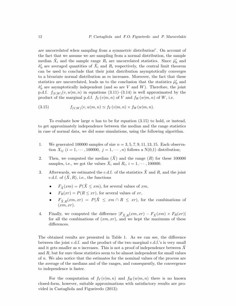
To evaluate how large n has to be for equation (3.15) to hold, or instead,to get approximately independence between the median and the range statisticsin case of normal data, we did some simulations, using the following algorithm.

1. We generated 100000 samples of size n = 3, 5, 7, 9, 11, 13, 15. Each observa-tion Xij (i = 1, · · · , 100000, j = 1, · · · , n) follows a N(0,1) distribution;

2. Then, we computed the median (X) and the range (R) for these 100000samples, i.e., we got the values Xi and Ri, i = 1, · · · , 100000.

3. Afterwards, we estimated the c.d.f. of the statistics X and R, and the jointc.d.f. of (X, R), i.e., the functions

• FX(xm) = P (X ≤ xm), for several values of xm,

• FR(xr) = P (R ≤ xr), for several values of xr,

• FX,R(xm, xr) = P (X ≤ xm ∩ R ≤ xr), for the combinations of(xm, xr).

4. Finally, we computed the difference |FX,R(xm, xr) − FX(xm) × FR(xr)|for all the combinations of (xm, xr), and we kept the maximum of thesedifferences.

The obtained results are presented in Table 1. As we can see, the differencebetween the joint c.d.f. and the product of the two marginal c.d.f.’s is very smalland it gets smaller as n increases. This is not a proof of independence between Xand R, but for sure these statistics seem to be almost independent for small valuesof n. We also notice that the estimates for the nominal values of the process arethe average of the medians and of the ranges, and consequently, the convergenceto independence is faster.

For the computation of fV (v|m,n) and fW (w|m,n) there is no knownclosed-form, however, suitable approximations with satisfactory results are pro-vided in Castagliola and Figueiredo (2013):


Sample size n max |FX,R(xm, xr)− FX(xm)× FR(xr)|3 0.011345 0.008387 0.006409 0.0052911 0.0048113 0.0040215 0.00402

Table 1: Maximum difference between the joint c.d.f. and the product ofthe two marginal c.d.f. for some small sample sizes n.

• the marginal p.d.f. fV (v|m,n), can be computed through the equation

fV (v|m,n) ' b√(v − δ)2 + d2

φ

(b sinh−1

(v − δd

)),

where φ(x) is the p.d.f. of the standard normal distribution, and

b =

√2

ln(√

2(γ2(V ) + 2)− 1),

d =

√2µ2(V )√

2(γ2(V ) + 2)− 2,

with

µ2(V ) ' 1

m

(π

2(n+ 2)+

π2

4(n+ 2)2+π2(1324π − 1

)2(n+ 2)3

),

γ2(V ) ' 2(π − 3)

m(n+ 2);

• the marginal p.d.f. fW (w|m,n), can be computed through the equation

fW (w|m,n) ' 2νd22(n)w

c2fχ2

(νd22(n)w2

c2|ν),

where fχ2(x|ν) is the p.d.f. of the χ2 distribution with ν degrees of freedomwith

ν '

−2 + 2

√√√√√√1 + 2

B

A2+

(−2 + 2

√1 + 2B

A2

)316

−1

,

c ' A

(1 +

1

4ν+

1

32ν2− 1

128ν3

),

and A = d2(n), B =d23(n)m where d2(n) and d3(n) are constants tabulated

for the normal case.


4. A COMPARISON

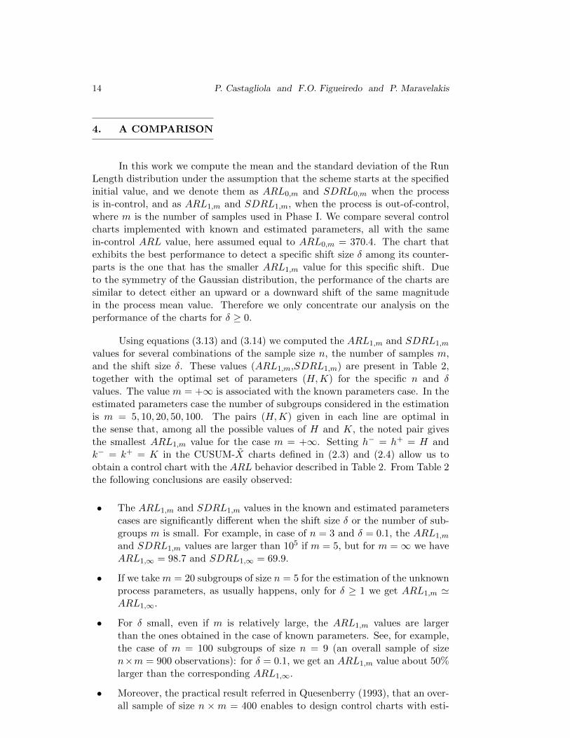
In this work we compute the mean and the standard deviation of the RunLength distribution under the assumption that the scheme starts at the specifiedinitial value, and we denote them as ARL0,m and SDRL0,m when the processis in-control, and as ARL1,m and SDRL1,m, when the process is out-of-control,where m is the number of samples used in Phase I. We compare several controlcharts implemented with known and estimated parameters, all with the samein-control ARL value, here assumed equal to ARL0,m = 370.4. The chart thatexhibits the best performance to detect a specific shift size δ among its counter-parts is the one that has the smaller ARL1,m value for this specific shift. Dueto the symmetry of the Gaussian distribution, the performance of the charts aresimilar to detect either an upward or a downward shift of the same magnitudein the process mean value. Therefore we only concentrate our analysis on theperformance of the charts for δ ≥ 0.

Using equations (3.13) and (3.14) we computed the ARL1,m and SDRL1,m

values for several combinations of the sample size n, the number of samples m,and the shift size δ. These values (ARL1,m,SDRL1,m) are present in Table 2,together with the optimal set of parameters (H,K) for the specific n and δvalues. The value m = +∞ is associated with the known parameters case. In theestimated parameters case the number of subgroups considered in the estimationis m = 5, 10, 20, 50, 100. The pairs (H,K) given in each line are optimal inthe sense that, among all the possible values of H and K, the noted pair givesthe smallest ARL1,m value for the case m = +∞. Setting h− = h+ = H andk− = k+ = K in the CUSUM-X charts defined in (2.3) and (2.4) allow us toobtain a control chart with the ARL behavior described in Table 2. From Table 2the following conclusions are easily observed:

• The ARL1,m and SDRL1,m values in the known and estimated parameterscases are significantly different when the shift size δ or the number of sub-groups m is small. For example, in case of n = 3 and δ = 0.1, the ARL1,m

and SDRL1,m values are larger than 105 if m = 5, but for m =∞ we haveARL1,∞ = 98.7 and SDRL1,∞ = 69.9.

• If we take m = 20 subgroups of size n = 5 for the estimation of the unknownprocess parameters, as usually happens, only for δ ≥ 1 we get ARL1,m 'ARL1,∞.

• For δ small, even if m is relatively large, the ARL1,m values are largerthan the ones obtained in the case of known parameters. See, for example,the case of m = 100 subgroups of size n = 9 (an overall sample of sizen×m = 900 observations): for δ = 0.1, we get an ARL1,m value about 50%larger than the corresponding ARL1,∞.

• Moreover, the practical result referred in Quesenberry (1993), that an over-all sample of size n ×m = 400 enables to design control charts with esti-


n = 3δ (H,K) m = 5 m = 10 m = 20 m = 50 m = 100 m =∞

0.1 (8.003, 0.0501) (> 105, > 105) (> 105, > 105) (> 105, > 105) (636.9, 60171.3) (165.7, 659.3) (98.7, 69.9)0.2 (6.003, 0.0999) (> 105, > 105) (> 105, > 105) (2723.1, > 105) (76.7, 407.1) (55.9, 66.2) (46.5, 30.4)0.3 (4.813, 0.1497) (> 105, > 105) (> 105, > 105) (98.3, 14407.4) (34.4, 49.9) (30.3, 25.5) (27.5, 17.1)0.5 (3.444, 0.2489) (> 105, > 105) (63.6, 62917.8) (17.7, 47.5) (14.5, 11.3) (13.9, 9.2) (13.3, 7.7)0.7 (2.666, 0.3478) (1039.6, > 105) (11.8, 165.9) (9.1, 8.6) (8.4, 5.5) (8.2, 4.9) (8.0, 4.4)1.0 (1.965, 0.4951) (8.3, 2204.2) (5.3, 5.7) (4.9, 3.3) (4.7, 2.7) (4.7, 2.6) (4.6, 2.4)1.5 (1.319, 0.7432) (2.8, 3.3) (2.6, 1.7) (2.5, 1.4) (2.5, 1.3) (2.5, 1.3) (2.5, 1.2)2.0 (0.934, 0.9963) (1.7, 1.1) (1.6, 0.9) (1.6, 0.8) (1.6, 0.8) (1.6, 0.8) (1.6, 0.8)

n = 5δ (H,K) m = 5 m = 10 m = 20 m = 50 m = 100 m =∞

0.1 (5.903, 0.0500) (> 105, > 105) (> 105, > 105) (> 105, > 105) (275.2, 8232.2) (115.9, 281.0) (79.1, 54.7)0.2 (4.269, 0.0999) (> 105, > 105) (> 105, > 105) (266.2, 49881.9) (48.3, 107.4) (39.9, 38.2) (35.1, 22.2)0.3 (3.349, 0.1496) (> 105, > 105) (829.8, > 105) (37.1, 474.7) (23.4, 23.6) (21.6, 16.0) (20.2, 12.1)0.5 (2.329, 0.2487) (1035.0, > 105) (16.5, 316.0) (11.3, 12.8) (10.1, 6.9) (9.8, 6.0) (9.5, 5.3)0.7 (1.767, 0.3473) (14.5, 3462.5) (6.9, 10.9) (6.2, 4.5) (5.9, 3.5) (5.8, 3.2) (5.7, 3.0)1.0 (1.270, 0.4949) (4.1, 11.7) (3.6, 2.6) (3.4, 2.0) (3.3, 1.8) (3.3, 1.7) (3.3, 1.7)1.5 (0.812, 0.7467) (1.9, 1.3) (1.8, 1.0) (1.8, 0.9) (1.8, 0.9) (1.8, 0.9) (1.7, 0.9)2.0 (0.511, 0.9990) (1.3, 0.6) (1.2, 0.5) (1.2, 0.5) (1.2, 0.5) (1.2, 0.5) (1.2, 0.4)

n = 7δ (H,K) m = 5 m = 10 m = 20 m = 50 m = 100 m =∞

0.1 (4.749, 0.0500) (> 105, > 105) (> 105, > 105) (27291.2, > 105) (170.3, 2633.7) (90.9, 166.3) (67.0, 45.5)0.2 (3.348, 0.0999) (> 105, > 105) (17933.4, > 105) (100.8, 5616.9) (36.2, 54.4) (31.6, 27.1) (28.6, 17.8)0.3 (2.586, 0.1496) (> 105, > 105) (123.7, 36763.2) (24.0, 102.8) (18.0, 15.6) (17.0, 11.8) (16.2, 9.5)0.5 (1.762, 0.2487) (60.7, 50167.3) (10.5, 42.8) (8.5, 7.4) (7.8, 5.0) (7.7, 4.5) (7.5, 4.1)0.7 (1.316, 0.3472) (7.0, 114.4) (5.1, 4.9) (4.7, 3.1) (4.6, 2.6) (4.5, 2.5) (4.5, 2.3)1.0 (0.926, 0.4963) (3.0, 3.3) (2.7, 1.8) (2.6, 1.5) (2.6, 1.4) (2.6, 1.3) (2.6, 1.3)1.5 (0.557, 0.7484) (1.5, 0.8) (1.4, 0.7) (1.4, 0.7) (1.4, 0.6) (1.4, 0.6) (1.4, 0.6)2.0 (0.286, 0.9998) (1.1, 0.3) (1.1, 0.3) (1.1, 0.3) (1.1, 0.3) (1.1, 0.3) (1.1, 0.3)

n = 9δ (H,K) m = 5 m = 10 m = 20 m = 50 m = 100 m =∞

0.1 (4.007, 0.0500) (> 105, > 105) (> 105, > 105) (7728.6, > 105) (123.1, 1171.1) (75.7, 115.1) (58.7, 39.3)0.2 (2.770, 0.0999) (> 105, > 105) (2714.7, > 105) (58.7, 1396.9) (29.4, 35.5) (26.4, 21.0) (24.3, 14.9)0.3 (2.114, 0.1496) (24658.7, > 105) (48.4, 4394.4) (18.2, 42.2) (14.8, 11.7) (14.2, 9.4) (13.6, 7.9)0.5 (1.416, 0.2487) (19.3, 2775.4) (7.9, 15.3) (6.9, 5.3) (6.5, 4.0) (6.4, 3.6) (6.3, 3.4)0.7 (1.044, 0.3474) (5.0, 20.6) (4.1, 3.3) (3.9, 2.4) (3.8, 2.1) (3.7, 2.0) (3.7, 1.9)1.0 (0.721, 0.4976) (2.4, 2.0) (2.2, 1.3) (2.2, 1.2) (2.2, 1.1) (2.1, 1.1) (2.1, 1.1)1.5 (0.399, 0.7493) (1.3, 0.6) (1.2, 0.5) (1.2, 0.5) (1.2, 0.5) (1.2, 0.5) (1.2, 0.5)2.0 (0.140, 0.9999) (1.0, 0.2) (1.0, 0.2) (1.0, 0.1) (1.0, 0.1) (1.0, 0.1) (1.0, 0.1)

Table 2: ARL1,m, SDRL1,m, H, K values for different combinations ofn, m and δ.

mated control limits with a similar performance to the corresponding chartwith true limits does not hold in the case of CUSUM-X charts (see, forinstance, the ARL1,m and SDRL1,m values for small values of δ and, inparticular, for δ = 0.1).

• However, as the number of samples m increases the ARL1,m and SDRL1,m

values converge to the values of the known parameters case, for each shift,although very slowly. In particular, when δ becomes large, the differencebetween the ARL1,m and SDRL1,m values in the known and estimatedparameters cases tends to be non-significant. But the CUSUM charts aremore attractive and efficient than the Shewhart charts for detecting smallchanges, and thus, it is important to determine optimal parameters H ′ andK ′ in order to guarantee the desired performance even for m or δ small.


For completeness, in Table 3 we also present the in-control ARL0,m andSDRL0,m values for the same pairs (H,K) considered in Table 2. As in Table 2,we observe again that, as m increases, the ARL0,m and SDRL0,m values convergevery slowly to the known parameters case values. As we can observe more thanm = 100 samples are often needed to implement charts with known and estimatedparameters with similar performance.

n = 3(H,K) m = 5 m = 10 m = 20 m = 50 m = 100

(8.003, 0.0501) (> 105, > 105) (> 105, > 105) (> 105, > 105) (15540.8, > 105) (1429.9, 16918.4)(6.003, 0.0999) (> 105, > 105) (> 105, > 105) (> 105, > 105) (2989.3, > 105) (865.0, 3768.4)(4.813, 0.1497) (> 105, > 105) (> 105, > 105) (70529.8, > 105) (1517.3, 17422.5) (682.9, 1905.6)(3.444, 0.2489) (> 105, > 105) (> 105, > 105) (5501.3, > 105) (853.9, 3474.9) (544.3, 1032.7)(2.666, 0.3478) (> 105, > 105) (48309.8, > 105) (2109.7, 49864.4) (663.5, 1754.4) (488.1, 777.8)(1.965, 0.4951) (> 105, > 105) (5812.4, > 105) (1114.4, 7639.5) (548.4, 1066.1) (447.5, 622.0)(1.319, 0.7432) (20921.5, > 105) (1593.5, 24654.9) (704.3, 2093.0) (470.9, 717.4) (416.6, 515.1)(0.934, 0.9963) (3608.3, > 105) (952.1, 4648.1) (572.8, 1184.7) (437.6, 587.0) (402.1, 466.6)

n = 5(H,K) m = 5 m = 10 m = 20 m = 50 m = 100

(5.903, 0.0500) (> 105, > 105) (> 105, > 105) (> 105, > 105) (7577.1, > 105) (1192.1, 9102.0)(4.269, 0.0999) (> 105, > 105) (> 105, > 105) (> 105, > 105) (1883.9, 25530.6) (747.4, 2380.3)(3.349, 0.1496) (> 105, > 105) (> 105, > 105) (11797.0, > 105) (1092.2, 6198.7) (605.9, 1346.7)(2.329, 0.2487) (> 105, > 105) (33318.5, > 105) (2239.1, 38019.5) (691.1, 1873.1) (498.4, 812.6)(1.767, 0.3473) (> 105, > 105) (5584.4, > 105) (1183.7, 7401.6) (565.8, 1128.0) (454.9, 643.8)(1.270, 0.4949) (17364.4, > 105) (1774.2, 22295.1) (756.6, 2351.7) (485.6, 767.9) (423.1, 534.6)(0.812, 0.7467) (2555.9, 62815.4) (872.2, 3340.4) (555.7, 1078.3) (433.5, 571.3) (400.4, 461.0)(0.511, 0.9990) (1497.0, 14155.3) (696.7, 1890.8) (500.9, 824.3) (416.6, 511.7) (392.6, 435.7)

n = 7(H,K) m = 5 m = 10 m = 20 m = 50 m = 100

(4.749, 0.0500) (> 105, > 105) (> 105, > 105) (> 105, > 105) (5134.7, > 105) (1060.8, 6361.6)(3.348, 0.0999) (> 105, > 105) (> 105, > 105) (33886.4, > 105) (1474.5, 12982.1) (683.9, 1848.5)(2.586, 0.1496) (> 105, > 105) (> 105, > 105) (5777.0, > 105) (918.3, 3825.0) (564.8, 1115.2)(1.762, 0.2487) (> 105, > 105) (10278.2, > 105) (1538.4, 13243.4) (619.3, 1401.7) (474.6, 715.3)(1.316, 0.3472) (48309.2, > 105) (2766.0, 57099.5) (921.1, 3705.8) (521.7, 913.9) (438.0, 583.3)(0.926, 0.4963) (4897.4, > 105) (1170.3, 6580.6) (638.6, 1505.7) (457.4, 656.4) (411.1, 495.0)(0.557, 0.7484) (1671.5, 17793.4) (734.8, 2135.8) (514.2, 880.8) (421.0, 526.9) (394.7, 442.4)(0.286, 0.9998) (1282.1, 9130.3) (652.2, 1599.9) (485.7, 760.6) (411.7, 494.9) (390.3, 428.3)

n = 9(H,K) m = 5 m = 10 m = 20 m = 50 m = 100

(4.007, 0.0500) (> 105, > 105) (> 105, > 105) (> 105, > 105) (3935.5, > 105) (974.1, 4940.8)(2.770, 0.0999) (> 105, > 105) (> 105, > 105) (17455.0, > 105) (1253.9, 8409.7) (642.6, 1558.6)(2.114, 0.1496) (> 105, > 105) (> 105, > 105) (3795.7, > 105) (819.6, 2826.8) (538.3, 983.3)(1.416, 0.2487) (> 105, > 105) (5549.9, > 105) (1230.8, 7364.1) (576.9, 1169.2) (459.4, 657.7)(1.044, 0.3474) (14888.5, > 105) (1880.1, 19722.5) (790.3, 2495.0) (494.9, 799.0) (427.2, 546.5)(0.721, 0.4976) (2879.4, 59731.6) (946.2, 3818.3) (580.8, 1186.6) (441.5, 598.3) (404.1, 472.5)(0.399, 0.7493) (1428.2, 11824.2) (685.3, 1800.5) (497.4, 808.7) (415.6, 508.2) (392.2, 434.3)(0.140, 0.9999) (1233.9, 8245.2) (641.1, 1533.9) (481.7, 744.4) (410.4, 490.3) (389.7, 426.3)

Table 3: ARL0,m, SDRL0,m, H, K values for several pairs of n and mwhen the process is in-control.

Since the out-of-control ARL1,m values are clearly different in the knownand in the estimated parameters case, it is important to determine the numberm of Phase I samples we should consider to get approximately the same out-of-control ARL1,m values in both cases, using the same optimal control chartparameters H and K displayed in Table 2. Thus, with

∆ =|ARL1,m −ARL1,∞|

ARL1,∞


denoting the relative difference between the out-of-control ARL1,m (esti-mated parameter case) and ARL1,∞ (known parameter case) values, we computedthe minimum value of m satisfying ∆ ≤ 0.05 or ∆ ≤ 0.01. The obtained mini-mum number m of Phase I samples is given in Table 4 for some values of n andδ. From this table we observe that:

• The value of m satisfying ∆ < 0.05 or ∆ < 0.01 can be very large, forinstance, m > 100 if δ ≤ 0.3. In particular, for δ = 0.1 and n = 9, to have∆ < 0.05 we must consider at least 417 samples.

• For the most common subgroup sample size n = 5, the number of subgroupsmust be 569 for very small shifts (say, for δ = 0.1), and consequently n×mwill be 2845, much larger than 400, as suggested by Quesenberry (1993).

• The number of the required samples decreases with the increase shift size δ.We also observe that the number of subgroups m that are needed decreaseswith the sample size n, but the number of observations of the overall sampleneeded for the estimation, n×m, also increases.

∆ = (0.05, 0.01)δ n = 3 n = 5 n = 7 n = 9

0.1 (711, 3339) (569, 2669) (479, 2241) (417, 1945)0.2 (319, 1485) (237, 1101) (191, 881) (159, 737)0.3 (181, 835) (129, 597) (101, 467) (83, 385)0.5 (81, 371) (55, 257) (43, 197) (35, 159)0.7 (45, 209) (31, 141) (23, 107) (19, 87)1.0 (25, 109) (17, 73) (13, 55) (9, 45)1.5 (11, 51) (7, 35) (5, 27) (5, 21)2.0 (7, 33) (5, 21) (3, 11) (3, 5)

Table 4: Minimum number m of Phase I samples required to satisfy ∆ =0.05 (left value) and ∆ = 0.01 (right value) when the process isout of control.

As a conclusion, we observe that in most of the cases a very large numberm of Phase I samples is needed so that the charts with known and estimatedparameters have the same ARL performance. But this requirement is in generalvery hard to handle in practice for economical and logistic reasons. Therefore, forfixed values of m and n, the determination of adequate control chart parameters,taking into consideration the variability introduced by the parameters estimationis very challenging.

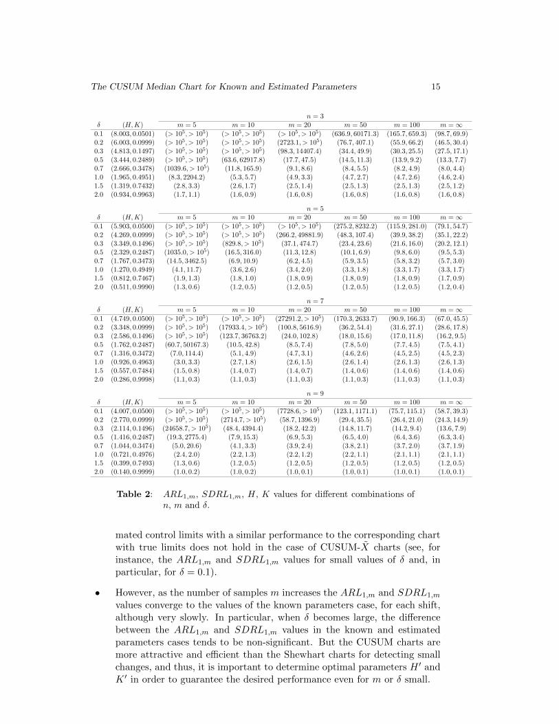
In this paper we computed, for fixed values of m and n, new chart param-eters denoted as (H ′,K ′), in order to achieve the desired in-control performance,i.e. such that, for fixed values of m and n, we have ARL(m,n,H ′,K ′, δ = 0) =370.4 and, for a fixed value of δ, ARL(m,n,H ′,K ′, δ) is the smallest out-of-controlARL1,m. These new pairs of constants are given in Tables 5 and 6 for various


combinations of n, m and δ, and might be used as the chart parameters in theCUSUM-X charts defined in (3.8) and (3.7), i.e., we might choose h−g = h+g = H ′

and k−g = k+g = K ′. In each cell of Tables 5 and 6, the two numbers in thefirst row are new chart parameters (H ′,K ′), and the two numbers in the sec-ond row are the ARL1,m and SDRL1,m values. As we can observe, with theseconstants (H ′,K ′) determined with the unconditional run length distribution,we can guarantee the same performance of the corresponding chart implementedwith known process parameters, or even a better performance, except in the casesof m = 5, 10 and δ = 0.1. For the shift size δ that must be quickly detected, thevalues presented in Tables 5 and 6 allow the practitioners to easily implement themost efficient median CUSUM control chart. For instance, if n = 5 and m = 20,the optimal CUSUM-X chart to detect a shift of size δ = 1 must be designedwith the constants H ′ = 1.314 and K ′ = 0.40. With these chart parameters weget the values ARL1,m = 3 and SDRL1,m = 1.6.

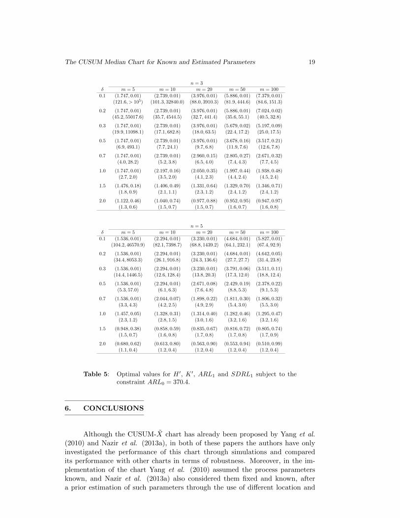
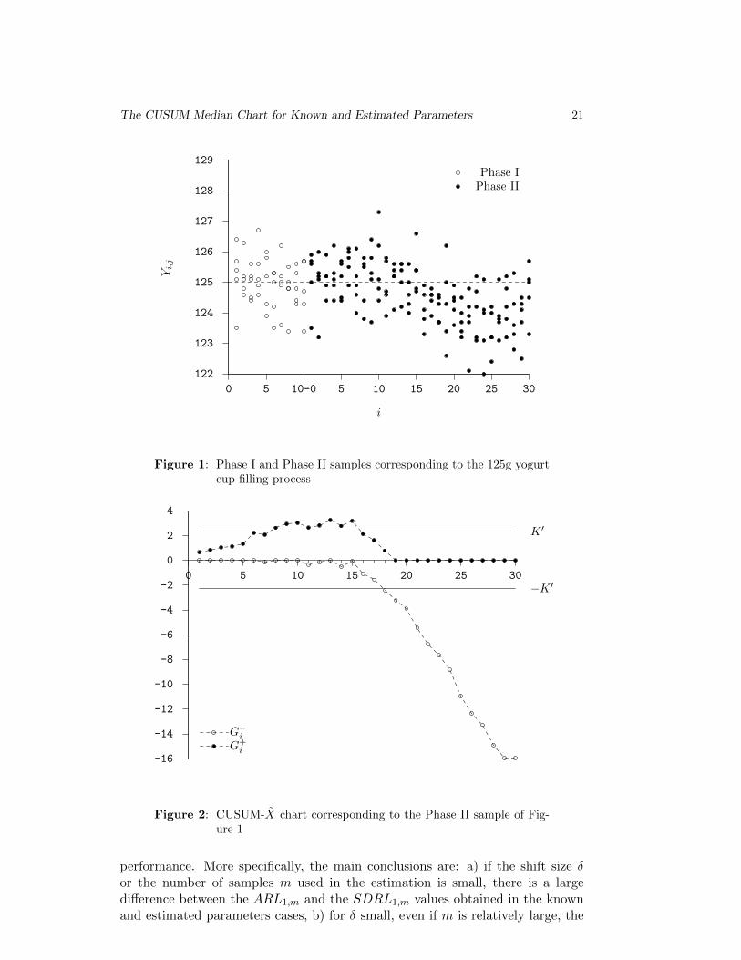
5. AN ILLUSTRATIVE EXAMPLE

In order to illustrate the use of the CUSUM-X chart when the parametersare estimated, let us consider the same example as the one in Castagliola andFigueiredo (2013), i.e. a 125g yogurt cup filling process for which the qualitycharacteristic Y is the weight of each yogurt cup. The Phase I dataset used inthis example consists of m = 10 subgroups of size n = 5 plotted in the left partof Figure 1 with “◦”. From this Phase I dataset, using (3.3) and (3.4), we obtainµ′0 = 125.02 and σ′0 = 0.864. According to the quality practitioner in chargeof this process, a shift of 0.5σ0 (i.e., δ = 0.5) in the process position should beinterpreted as a signal that something is going wrong in the production. Form = 10, n = 5 and δ = 0.5, Table 5 suggests to use K ′ = 2.294 and H ′ = 0.01.

The Phase II dataset used in this example consists of m = 30 subgroups ofsize n = 5 plotted in the right part of Figure 1 with “•”. The first 15 subgroupsare supposed to be in-control while the last 15 subgroups are supposed to have asmaller yogurt weight, and thus, to be out-of-control. In Figure 2, we plotted thestatistics G−i and G+

i corresponding to (3.5) and (3.6). This figure shows that the7th first subgroups are in-control but, from subgroups #8 to #15, the processexperiences a light out-of-control situation (increase) as the points “•” corre-sponding to the G+

i ’s are above the upper limit K ′ = 2.294. During subgroups#16 and #17, the process returns to the in-control state but, as expected, sud-denly experiences a new strong out-of-control situation (decrease) as the points“◦” corresponding to the G−i ’s are now below the lower limit −K ′ = −2.294.


n = 3δ m = 5 m = 10 m = 20 m = 50 m = 100

0.1 (1.747, 0.01) (2.739, 0.01) (3.976, 0.01) (5.886, 0.01) (7.379, 0.01)(121.6, > 105) (101.3, 32840.0) (88.0, 3910.3) (81.9, 444.6) (84.6, 151.3)

0.2 (1.747, 0.01) (2.739, 0.01) (3.976, 0.01) (5.886, 0.01) (7.024, 0.02)(45.2, 55017.6) (35.7, 4544.5) (32.7, 441.4) (35.6, 55.1) (40.5, 32.8)

0.3 (1.747, 0.01) (2.739, 0.01) (3.976, 0.01) (5.679, 0.02) (5.197, 0.09)(19.9, 11098.1) (17.1, 682.8) (18.0, 63.5) (22.4, 17.2) (25.0, 17.5)

0.5 (1.747, 0.01) (2.739, 0.01) (3.976, 0.01) (3.678, 0.16) (3.517, 0.21)(6.9, 493.1) (7.7, 24.1) (9.7, 6.8) (11.9, 7.6) (12.6, 7.8)

0.7 (1.747, 0.01) (2.739, 0.01) (2.960, 0.15) (2.805, 0.27) (2.671, 0.32)(4.0, 28.2) (5.2, 3.8) (6.5, 4.0) (7.4, 4.3) (7.7, 4.5)

1.0 (1.747, 0.01) (2.197, 0.16) (2.050, 0.35) (1.997, 0.44) (1.938, 0.48)(2.7, 2.0) (3.5, 2.0) (4.1, 2.3) (4.4, 2.4) (4.5, 2.4)

1.5 (1.476, 0.18) (1.406, 0.49) (1.331, 0.64) (1.329, 0.70) (1.346, 0.71)(1.8, 0.9) (2.1, 1.1) (2.3, 1.2) (2.4, 1.2) (2.4, 1.2)

2.0 (1.122, 0.46) (1.040, 0.74) (0.977, 0.88) (0.952, 0.95) (0.947, 0.97)(1.3, 0.6) (1.5, 0.7) (1.5, 0.7) (1.6, 0.7) (1.6, 0.8)

n = 5δ m = 5 m = 10 m = 20 m = 50 m = 100

0.1 (1.536, 0.01) (2.294, 0.01) (3.230, 0.01) (4.684, 0.01) (5.827, 0.01)(104.2, 46570.9) (82.1, 7398.7) (68.8, 1439.2) (64.1, 232.1) (67.4, 92.9)

0.2 (1.536, 0.01) (2.294, 0.01) (3.230, 0.01) (4.684, 0.01) (4.642, 0.05)(34.4, 8053.3) (26.1, 916.8) (24.3, 136.6) (27.7, 27.7) (31.4, 23.8)

0.3 (1.536, 0.01) (2.294, 0.01) (3.230, 0.01) (3.791, 0.06) (3.511, 0.11)(14.4, 1446.5) (12.6, 128.4) (13.8, 20.3) (17.3, 12.0) (18.8, 12.4)

0.5 (1.536, 0.01) (2.294, 0.01) (2.671, 0.08) (2.429, 0.19) (2.378, 0.22)(5.3, 57.0) (6.1, 6.3) (7.6, 4.8) (8.8, 5.3) (9.1, 5.3)

0.7 (1.536, 0.01) (2.044, 0.07) (1.898, 0.22) (1.811, 0.30) (1.806, 0.32)(3.3, 4.3) (4.2, 2.5) (4.9, 2.9) (5.4, 3.0) (5.5, 3.0)

1.0 (1.457, 0.05) (1.328, 0.31) (1.314, 0.40) (1.282, 0.46) (1.295, 0.47)(2.3, 1.2) (2.8, 1.5) (3.0, 1.6) (3.2, 1.6) (3.2, 1.6)

1.5 (0.948, 0.38) (0.858, 0.59) (0.835, 0.67) (0.816, 0.72) (0.805, 0.74)(1.5, 0.7) (1.6, 0.8) (1.7, 0.8) (1.7, 0.8) (1.7, 0.9)

2.0 (0.680, 0.62) (0.613, 0.80) (0.563, 0.90) (0.553, 0.94) (0.510, 0.99)(1.1, 0.4) (1.2, 0.4) (1.2, 0.4) (1.2, 0.4) (1.2, 0.4)

Table 5: Optimal values for H ′, K ′, ARL1 and SDRL1 subject to theconstraint ARL0 = 370.4.

6. CONCLUSIONS

Although the CUSUM-X chart has already been proposed by Yang et al.(2010) and Nazir et al. (2013a), in both of these papers the authors have onlyinvestigated the performance of this chart through simulations and comparedits performance with other charts in terms of robustness. Moreover, in the im-plementation of the chart Yang et al. (2010) assumed the process parametersknown, and Nazir et al. (2013a) also considered them fixed and known, aftera prior estimation of such parameters through the use of different location and


n = 7δ m = 5 m = 10 m = 20 m = 50 m = 100

0.1 (1.355, 0.01) (1.988, 0.01) (2.771, 0.01) (3.987, 0.01) (4.940, 0.01)(88.9, 19453.2) (67.5, 3754.2) (56.1, 844.7) (53.4, 147.8) (57.2, 65.7)

0.2 (1.355, 0.01) (1.988, 0.01) (2.771, 0.01) (3.987, 0.01) (3.597, 0.06)(26.4, 2921.9) (20.2, 389.8) (19.6, 65.3) (23.3, 18.3) (26.0, 18.5)

0.3 (1.355, 0.01) (1.988, 0.01) (2.771, 0.01) (2.862, 0.08) (2.671, 0.12)(10.8, 464.4) (10.1, 48.2) (11.6, 10.9) (14.2, 9.4) (15.2, 9.7)

0.5 (1.355, 0.01) (1.988, 0.01) (1.917, 0.13) (1.842, 0.20) (1.829, 0.22)(4.3, 16.0) (5.2, 3.5) (6.3, 3.9) (7.0, 4.1) (7.3, 4.1)

0.7 (1.355, 0.01) (1.488, 0.14) (1.397, 0.25) (1.346, 0.31) (1.326, 0.33)(2.9, 2.0) (3.6, 2.0) (4.0, 2.2) (4.3, 2.3) (4.4, 2.3)

1.0 (1.038, 0.18) (0.997, 0.34) (0.943, 0.43) (0.933, 0.47) (0.936, 0.48)(2.0, 1.1) (2.3, 1.2) (2.4, 1.3) (2.5, 1.3) (2.5, 1.3)

1.5 (0.668, 0.46) (0.600, 0.62) (0.573, 0.69) (0.581, 0.71) (0.568, 0.73)(1.3, 0.5) (1.3, 0.6) (1.4, 0.6) (1.4, 0.6) (1.4, 0.6)

2.0 (0.429, 0.69) (0.386, 0.82) (0.316, 0.93) (0.320, 0.95) (0.318, 0.96)(1.0, 0.2) (1.1, 0.2) (1.1, 0.2) (1.1, 0.2) (1.1, 0.2)

n = 9δ m = 5 m = 10 m = 20 m = 50 m = 100

0.1 (1.220, 0.01) (1.774, 0.01) (2.459, 0.01) (3.521, 0.01) (4.350, 0.01)(76.9, 11291.0) (57.1, 2426.2) (47.5, 568.6) (46.4, 103.4) (50.3, 50.5)

0.2 (1.220, 0.01) (1.774, 0.01) (2.459, 0.01) (3.143, 0.03) (2.889, 0.07)(21.0, 1482.2) (16.5, 210.2) (16.7, 37.5) (20.3, 15.3) (22.4, 15.5)

0.3 (1.220, 0.01) (1.774, 0.01) (2.459, 0.01) (2.226, 0.10) (2.224, 0.12)(8.6, 208.6) (8.6, 23.5) (10.1, 7.4) (12.2, 8.0) (12.9, 7.8)

0.5 (1.220, 0.01) (1.685, 0.03) (1.532, 0.15) (1.465, 0.21) (1.438, 0.23)(3.8, 6.7) (4.6, 2.7) (5.4, 3.2) (5.9, 3.3) (6.1, 3.4)

0.7 (1.220, 0.01) (1.164, 0.18) (1.095, 0.27) (1.056, 0.32) (1.061, 0.33)(2.6, 1.4) (3.1, 1.7) (3.4, 1.8) (3.6, 1.9) (3.6, 1.9)

1.0 (0.825, 0.23) (0.758, 0.38) (0.724, 0.45) (0.736, 0.47) (0.735, 0.48)(1.8, 0.9) (1.9, 1.0) (2.0, 1.1) (2.1, 1.1) (2.1, 1.1)

1.5 (0.519, 0.48) (0.446, 0.63) (0.401, 0.71) (0.382, 0.75) (0.379, 0.76)(1.1, 0.4) (1.2, 0.4) (1.2, 0.5) (1.2, 0.5) (1.2, 0.5)

2.0 (0.315, 0.68) (0.250, 0.82) (0.205, 0.90) (0.206, 0.92) (0.213, 0.92)(1.0, 0.1) (1.0, 0.1) (1.0, 0.1) (1.0, 0.1) (1.0, 0.1)

Table 6: (Cont’d) Optimal values for H ′, K ′, ARL1 and SDRL1 subjectto the constraint ARL0 = 370.4.

scale estimators. But they really did not analyze the effect of the parametersestimation in the performance of the chart in comparison with the performanceof the corresponding chart implemented with true parameters, the main objec-tive of our paper. We used a Markov chain methodology to compute the runlength distribution and the moments of the CUSUM-X chart in order to studyits performance when the parameters are known and estimated. In this paperwe present several tables that allow us to observe that the chart implementedwith estimated parameters exhibits a completely different performance in com-parison to the one of the chart implemented with known parameters. We alsoprovide modified chart parameters that allow the practitioners to implement theCUSUM-X chart with estimated control limits with a given desired in-control


122

123

124

125

126

127

128

129

0 5 10-0 5 10 15 20 25 30

Yi,j

i

Phase IPhase II

Figure 1: Phase I and Phase II samples corresponding to the 125g yogurtcup filling process

-16

-14

-12

-10

-8

-6

-4

-2

0

2

4

0 5 10 15 20 25 30

K ′

−K ′

G−iG+

i

Figure 2: CUSUM-X chart corresponding to the Phase II sample of Fig-ure 1

performance. More specifically, the main conclusions are: a) if the shift size δor the number of samples m used in the estimation is small, there is a largedifference between the ARL1,m and the SDRL1,m values obtained in the knownand estimated parameters cases, b) for δ small, even if m is relatively large, the


ARL1,m values are larger than the ones obtained in the case of known parame-ters, c) the ARL1,m and SDRL1,m values converge to the values of the knownparameters case as the number of samples m increases, d) the number of sub-groups m to have a relative difference between the out-of-control ARL values inthe known and estimated parameters cases less than 5% or 1% can be very large,and depends on the value of δ, e) it is possible to obtain new chart parameters inorder to achieve a desired in-control performance. As a general conclusion, theCUSUM-X chart can be a valuable alternative chart for practitioners since it issimpler than the CUSUM-X chart. The fact that it is robust against outliers,contamination or small deviations from normality is another advantage.

ACKNOWLEDGMENTS

Research partially supported by National Funds through FCT—Fundacaopara a Ciencia e a Tecnologia, project UID/MAT/00006/2013 (CEA/UL).We also acknowledge the valuable suggestions from a referee.

References

[1] Abujiya, M.R., Lee, M.H. and Riaz, M. (2015). Increasing the sen-sitivity of cumulative sum charts for location. Quality Reliability and En-gineering International, 31, 1035–1051.

[2] Al-Sabah, W.S. (2010) Cumulative sum statistical control charts usingranked set sampling data. Pakistan Journal of Statistics, 26, 2, 365-378.

[3] Brook, D. and Evans, D.A. (1972). An approach to the probabilitydistribution of CUSUM run length. Biometrika, 59, 3, 539-549.

[4] Castagliola, P. and Vannman, K. (2008). Average run length whenmonitoring capability indices using EWMA. Quality and Reliability Euro-pean Engineering International, 24, 8, 941-955.

[5] Castagliola, P. and Figueiredo, F.O. (2013). The median chartwith estimated parameters. European Journal of Industrial Engineering,7, 5, 594-614.

[6] Castagliola, P., Maravelakis, P., Psarakis, S. and Vannman, K.(2009). Monitoring capability indices using run rules. Journal of Qualityin Maintenance Engineering, 15, 4, 358-370.


[7] Chatterjee, S. and Qiu, P. (2009). Distribution-free cumulative sumcontrol charts using bootstrap-based control limits. Annals of AppliedStatistics, 3, 349–369.

[8] Chowdhury, S., Mukherjee A. and Chakraborti, S. (2015). Distri-bution free phase II CUSUM control chart for joint monitoring of locationand scale. Quality and Reliability Engineering International, 31, 1, 135–151.

[9] Gandy, A. and Kvaloy, J.T. (2013). Guaranteed conditional perfor-mance of control charts via bootstrap methods. Scandinavian Journal ofStatistics, 40, 647–668.

[10] Graham, M.A., Chackraborti, S. and Mukherjee, A. (2014). De-sign and implementation of CUSUM exceedance control charts for un-known location. International Journal of Production Research, 52, 5546–5564.

[11] Hawkins, D.M. and Olwell, D.H. (1999). Cumulative Sum Chartsand Charting for Quality Improvement. Springer-Verlag New York, Inc..

[12] He, F., Shu, L. and Tsui, K-L. (2014). Adaptive CUSUM charts formonitoring linear drifts in Poisso rates. International Journal of Produc-tion Economics, 148, 14–20.

[13] Hogg, R.V. (1960). Certain uncorrelated statistics. Journal of the Amer-ican Statistical Association, 55, 290, 265-267.

[14] Jensen, W.A., Jones-Farmer, L.A., Champ, C.W. and Woodall,W.H. (2006). Effects of parameter estimation on control chart properties:A literature review. Journal of Quality Technology, 38, 349–364.

[15] Latouche, G. and Ramaswami, V. (1999). Introduction to MatrixAnalytic Methods in Stochastic Modelling. ASA SIAM.

[16] Li, Z. and Wang, Z. (2010). Adaptive CUSUM of the Q chart. Inter-national Journal of Production Research, 48, 5, 1287–1301.

[17] Li, Z., Luo, Y. and Wang, Z. (2010a). CUSUM of Q chart with variablesampling intervals for monitoring the process mean. International Journalof Production Research, 48, 16, 4861–4876.

[18] Li, S-Y, Tang, L.C. and Ng S-H. (2010b). Nonparametric CUSUMand EWMA control charts for detecting mean shifts. Journal of QualityTechnology, 42, 2, 209–226.

[19] Liu, L., Tsung, F. and Zhang, J. (2014). Adaptive nonparamet-ric cusum scheme for detecting unknown shifts in location. InternationalJournal of Production Research, 52, 6, 1592-1606.


[20] Lombard, F., Hawkins, D.M. and Potgieter, C.J. (2017). Sequen-tial rank CUSUM charts for angular data. Computational Statistics andData Analysis, 105, 268-279.

[21] Montgomery, D.C. (2009). Introduction to Statistical Quality Control,6th edition. John Wiley & Sons, Inc..

[22] Mukherjee, A., Graham, M.A. and Chakraborti, S. (2013). Dis-tribution free exceedance CUSUM control charts for location. Communi-cations in Statistics - Simulation and Computation, 42, 5, 1153–1187.

[23] Nazir, H.Z., Riaz, M., Does, R.J.M.M. and Abbas, N. (2013a).Robust cusum control charting. Quality Engineering, 25, 3, 211-224.

[24] Nazir, H.Z., Riaz, M. and Does, R.J.M.M. (2013b). Robust CUSUMcontrol charting for process dispersion. Quality Reliability and EngineeringInternational, 31, 369-379.

[25] Nenes, G. and Tagaras, G. (2006). The economically designed cusumchart for monitoring short production runs. International Journal of Pro-duction Research, 44, 8, 1569-1587.

[26] Neuts, M.F. (1981). Matrix-Geometric Solutions in Stochastic Models:an Algorithmic Approach. Dover Publications Inc..

[27] Ou, Y., Wu, Z. and Tsung, F. (2011). A comparison study of effec-tiveness and robustness of control charts for monitoring process mean.International Journal of Production Economics, 135, 479–490.

[28] Ou, Y., Wen, D., Wu, Z. and Khoo, M.B.C. (2012). A comparisonstudy on effectiveness and robustness of control charts for monitoring pro-cess mean and variance. Quality Reliability and Engineering International,28, 3–17.

[29] Ou, Y., Wu, Z., Lee, K.M. and Wu, K. (2013). An adaptive CUSUMchart with single sample size for monitoring process mean and variance.Quality Reliability and Engineering International, 29, 1027-1039.

[30] Page, E.S. (1954). Continuous inspection schemes. Biometrika, 41, 12,100-115.

[31] Psarakis, S., Vyniou, A.K, and Castagliola, P. (2014). Some re-cent developments on the effects of parameter estimation on control charts.Quality and Reliability Engineering International, 30, 8, 1113-1129.

[32] Qiu, P. and Zhang, J. (2015). On phase II SPC in cases when normalityis invalid. Quality Reliability and Engineering International, 31, 27–35.

[33] Quesenberry, C.P. (1993). The effect of sample size on estimated limitsfor X and x control charts. Journal of Quality Technology, 25, 4, 237-247.


[34] Rakitzis, A., Maravelakis, P. and Castagliola, P. (2016).CUSUM control charts for the monitoring of zero-Inflated Binomial Pro-cesses. Quality and Reliability Engineering International, 32, 2, 465-483.

[35] Ryu, J-H., Wan, H. and Kim, S. (2010). Optimal design of a CUSUMchart for a mean shift of unknown size. Journal of Quality Technology, 42,3, 1-16.

[36] Saghir, A. and Lin, Z. (2014). Cumulative sum charts for monitoringCOM-poisson processes. Computers and Industrial Engineering, 68, 65–77.

[37] Saleh, N.A., Zwetsloot, I.M., Mahmoud., M.A. and Woodall,W.H. (2016). CUSUM charts with controlled conditional performance un-der estimated parameters. Quality Engineering, 28, 4, 402–415.

[38] Saniga, E.M., McWilliams, T., Davis., D.J. and Lucas, J.M.(2006). Economic control chart policies for monitoring variables. Interna-tional Journal of Productivity and Quality Management, 1, 1, 116–138.

[39] Saniga, E., Lucas, J., Davis, D. and McWilliams, T. (2012). Eco-nomic control chart policies for monitoring variables when there are twocomponents of variance. In Frontiers in Statistical Quality (Lenz, Wilrichand Schmid, Eds.), 10, 1, 85–95.

[40] Teoh, W.L., Khoo, M.B.C., Castagliola, P. and S. Chakraborti,S. (2014). Optimal design of the double sampling X chart with estimatedparameters based on median run length. Computers & Industrial Engi-neering, 67, 104-115.

[41] Wang, T. and Huang, S. (2016). An adaptive multivariate CUSUMcontrol chart for signaling a range of location shifts. Communications inStatistics - Theory and Methods, 45, 16, 4673–4691.

[42] Wang, D., Zhang, L. and Xiong, Q. (2017). A non parametricCUSUM control chart based on the Mann-Whitney statistic. Communi-cations in Statistics - Theory and Methods, 46, 10, 4713–4725.

[43] Wu, Z., Jiao, J., Yang, M., Liu, Y. and Wang, Z. (2009). Anenhanced adaptive CUSUM control chart. IIE Transactions, 41, 642–653.

[44] Yang, L., Pai, S. and Wang, Y.R. (2010). A novel cusum mediancontrol chart. In Proceedings of the International MultiConference of En-gineers and Computer Scientists (IMECS), 3, 1707-1710.

the cusum median chart for known and estimated parameters · pdf filesearchers and...

Documents