the cyclical sine model explanation for climate change by
TRANSCRIPT

1
The Cyclical Sine Model Explanation for Climate Change
By D. E. Nierode, PhD
ABSTRACT
The world is besieged with warnings that Global Warming/Climate Change is an existential threat to the very
survival of Earth1. This calamity is attributed to excessive burning of hydrocarbons resulting in carbon dioxide
buildup in the atmosphere. It is believed that this gas accumulation along with other “greenhouse” gasses would
irreversibly alter the Earth’s ability to reflect sunlight back into outer space. Instead, the Sun’s energy would
accumulate near the Earth’s surface and dangerously raise its temperature2. Contrary to those who predict the
Earth’s near-term demise are those who believe that nothing at all is happening to the Earth. This latter group
have been labeled “deniers” by the Climate Change community. In between these two groups are those who
search for an explanation employing Socrates’ dictum to “follow the data wherever it may lead.” This paper will
show that Global Warming/Climate Change is underway on Earth now, but it is a totally natural occurrence with
a solid scientific and historical basis. The Earth is currently in the upswing part of its normal temperature cycle.
Very warm (Medieval Warming) and very cold (Little Ice Age) cycles have been documented on Earth for at least
the last 3,000 years. The best explanation for the Earth’s current temperature increases since 1850 is a
mathematical model called the Cyclical Sine Model. It will be seen that this model is based on diverse scientific
results pointing to repetitive very cold and extremely hot periods repeated about every 1,500 years3. The Earth’s
current warming will be followed by another very cold period. Around the year 2500 historians will need to
come up with a name for our current warming cycle. One choice might be the Narcissistic Warming for a time
when mankind actually believed that they were in control of the fate of planet Earth.
INTRODUCTION
Since 1850 Earth average temperatures have been measured annually. Fig. 1 shows the general upward trend
in the data4. There is some scatter in the overall upward trend, but in general, temperatures have increased
about 1.3° C. since 1850. At various times climatologists and other Earth scientists have noticed unusual trends
in the temperatures. From about 1945 to 1970 temperatures had leveled off and were somewhat decreasing,
leading to fears of an impending ice age5.
Fig. 1 Measured Earth Temperature Difference from the 20th Century Average of 14o C

2
A similar problem with the near term trends was realized by 2014 when it was noticed that temperatures again
seemed to be leveling off instead of increasing as predicted. Another ice age was not predicted then, instead
the temperature plateau from 1998 to 2014 was labeled the “hiatus”6 which led to discarding the term Global
Warming in favor of Climate Change.
The Cyclical Sine Model for Earth temperature variations will be seen to explain what has happened to Earth
well before 1850 and up to the present and predict what will happen in the future. Global Warming/Climate
Change is occurring only in the sense that Earth temperatures are currently increasing.
EARTH TEMPERATURES ARE INCREASING
The upward trend of Earth temperatures since measurements began around 1850 is real. In 1850 there were
relatively few measurement locations on both land and water. With the Earth covered over 70% by water,
ocean temperatures are especially important. Until about 1980, ocean temperatures were mostly measured by
ships with a bucket on a rope tossed overboard. There is even controversy over whether the bucket was made
of metal or leather. The ship’s position was determined in the past by celestial navigation and temperatures
were recorded on paper with analysis done later. Over time more land and water locations were added, and
analysis is now done by computer with data often transmitted by satellite. Ships who take in water to cool their
engines now suck it in from about 30 ft below their keel and measure the inlet temperature somewhere before
it performs its cooling task. Now we also have many buoys that communicate their temperatures by satellite.
About 70% of ocean temperature measurements now come from buoys. Some of the buoys are submersible
and resurface at regular intervals to transmit their data. In general, data from the last four or five decades are
probably more accurate than prior years. There is currently a controversy about what to do with ocean
temperatures as buoys report on average 0.12°C. colder values compared to ship data7. Right now, it seems
that buoy temperatures are increased to agree with the warmer ship data. This is not unreasonable since older
data did not have any buoy data. However, it would have been equally reasonable to lower all ocean
temperatures.
EARTH CYCLES
Many cycles of the Earth have been observed and documented, with many long ago discovered by astronomer
Milutin Milankovic. These cycles are generically referred to as Milankovic Cycles8. Table 1 lists just a few of
these endless Earth cycles. The 1,500 year temperature cycle supported by this work is included in this group.
Table 1 Earth Cycles
Technical Term Description Length, years Pacific Decadal Oscillation Monthly North Pacific surface
temperature variability 40-60
Atlantic Multidecadal Oscillation Varying North Atlantic surface temperature variability
60-80
Gleissberg cycle Sunspot activity 87
Devries-Suess cycle Cosmic rays-upper atmosphere 210
Bond Cycles Atlantic Drift Ice Studies 1,000-1,500
Earth Temperature cycles Cycle above and below 14° C. 1,500±500
Axial precession Wobbling of the axis 25,772
Axial tilt Obliquity – 22.1° to 24.5° 41,000
Orbital inclination Inclination of orbital ellipse 70,000
Apsidal precession Wobbling of orbital ellipse 112,000
Orbital eccentricity Non-circular orbit 413,000
3
With oceans covering over 70% of the Earth’s surface it is obvious that ocean temperatures are especially
important for calculation of average Earth temperature. Water movement is also important. Main interests are
centered on the Atlantic and Pacific Oceans. Flows and surface temperature changes in these oceans are
believed of particular importance for our climate. In the Atlantic Ocean water flows from the Caribbean to
Labrador on the surface and returns at depth. This movement is called the Atlantic Meridional Overturning
Circulation9 (AMOC) which is very much like a conveyor belt. With only a few decades of AMOC measurements
it is too soon to access its exact importance for our climate. However, the Atlantic Multidecadal Oscillation10
(AMO) which is a correlation of small changes in surface temperatures in the North Atlantic has a long history.
With a period of 60 to 80 years surface temperature changes are within a range of only about 1° F. Yet these
small changes are thought to affect our climate. There are also studies of North Atlantic ice rafting (Bond
Cycles11) during the Holocene geological period (last 12,000 years) that had initially reported a 1,470+500 year
cyclicity which has since been revised downward12 to about 1,000 years. The Pacific Ocean similarly has
correlated surface temperatures in the Pacific Decadal Oscillations (PDO)13 that also affect our climate.
Oceanographers and climatologists have differing opinions14-15 about just what these ocean phenomena mean
for Climate Change. This discussion of the many Earth cycles serves to complement the Earth temperature cycle
revealed in The Cyclical Models section where possible correlations will be seen.
THE CYCLICAL MODELS
The temperature values in Fig. 1 are not the only information about Earth’s past temperature behavior. The
Earth has historically been experiencing regular temperature cycles. This cycling has been well documented by
Singer and Avery in their book Unstoppable Global Warming Every 1,500 Years16. Data summarized in that book
show that many, diverse scientific studies have observed Earth temperatures cycling in about 1,500±500 year
intervals. One ice core from the Vostok glacier in Antarctica observed 1,500 year temperature cycles17 over
more than 150,000 years. Other technical investigations like near shore sediment core analysis, studies of coral
reefs, stalagmites, tree rings, iron filings, and fossilized pollen found the same 1,500 year temperature cycles18.
These studies infer effective or “proxy temperatures” which are not actual measured values but are
temperatures changes that explain the variations seen in their data analysis. These studies mostly observed
hotter or colder conditions. The cause of these 1,500 year cycles is believed19 to be solar activity. It is interesting
to note that the Gleissberg and DeVries-Suess cycles in Table 1 combine to yield a possible 1,470 year cycle20
attributed to the sun. This is independent support for the 1,500 year cycles found in the proxy temperature
studies.
For the next two centuries the Earth will continue to experience higher temperatures and unusual things will
happen. Areas away from the equator will experience increased migration and food production will migrate to
those areas also. We will experience many of the changes mankind lived through in a period known as the
Medieval Warming. Then, this warm, inviting place called Greenland was discovered by the Vikings who grew
crops there to feed their animals21. After our current warming the Earth will cool and experience a very cold
period like The Little Ice Age when the Thames River in London froze solid at least 23 times22 and has not done
so again since 1814. Londoners held “Frost Fairs” on the solid ice with even an elephant walking across. The
good news is that we now have huge amounts of energy for use during very warm and very cold periods.
4
A cyclical model should have its repeated period in the range of 1,000-2,000 years to be consistent with the
proxy data. The initial strategy for cyclical modeling is to start with an assumed sine wave amplitude for a
cyclical model and see where that leads.
Single Sine Wave Model
Cyclical behavior has long been modeled by a simple sine wave function like Eqn. 1 that can be applied for
temperature as a function of time.
T(t) = A sin(2πt/Ƭ+φ) (1)
To fit Earth temperature as a function of time to this sine wave we need the amplitude A, the period Ƭ, and the
phase φ. Amplitude is the height of the sine wave above and below a center line. Period is the length of the
wave for a single increase and decrease cycle. Phase is the placement of the entire wave along the time axis. A
computerized method called nonlinear regression finds these values by minimizing the differences between
data and model. Nonlinear regression programs try various combinations of the variables in an organized way
with the goal of making the deviations between data and model as small as possible. See Appendix A for more
details.
Single Sine Model with Fixed Amplitude
We do not know how much Earth temperature fell and rose from a mean value during the past five historical
epochs. A base assumption is that it was the same for each past epoch and the present cycle. A first guess from
looking at the temperature for 2020 of 14.88° C. is that it may rise to a final value of 16° C. at the next maximum.
The sine wave amplitude A would then be 2° C. to oscillate from a 14° C. standard baseline. For this case, the
regression values would be only the period Ƭ and phase φ. This first regression used only the temperature data
through 2014 to be on a par with the UNIPCC study. The data since 2015 have a different character that will be
discussed later. The regression results are shown in Fig. 2 and Table 2.
Fig. 2 Single Sine Cyclical Model Fit to Data and Past Epochs
5
Table 2 Single Sine Cyclical Model Parameters
Period, years 1,094 Calculated
Amplitude, deg C. 2.00 Assumed
Phase, radians 152.2 Calculated
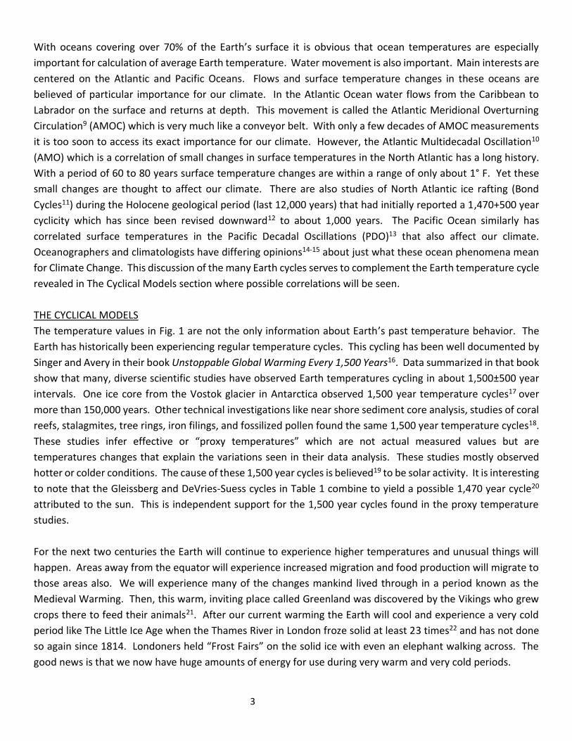
With the amplitude fixed at 2° C. every 1,094 years this heating and cooling cycle repeats itself. It is seen that
the last five climate change cycles in recorded history agree well in timing with this model. To the naked eye
the fit to measured temperatures looks reasonable, while the agreement with the past five climatic epochs is
exceptionally good. The Little Ice Age, Medieval Warming, and the other three epochs in historical documents
give confidence that current Earth behavior agrees with its own history. To include these historic cycles, it was
assumed that at the midpoint of each epoch the respective maximum or minimum temperature was reached.
This single large data point for each epoch is shown in Fig. 2. All these data together yield the Single Sine Cyclical
Model with fixed amplitude shown in Fig. 2 where the next maximum temperature is expected about 200 years
from now in the year 2220 after a further temperature increase of about 1.12°C. to the 16° C. maximum value.
Total increase since 1850 would be about 2.45° C.
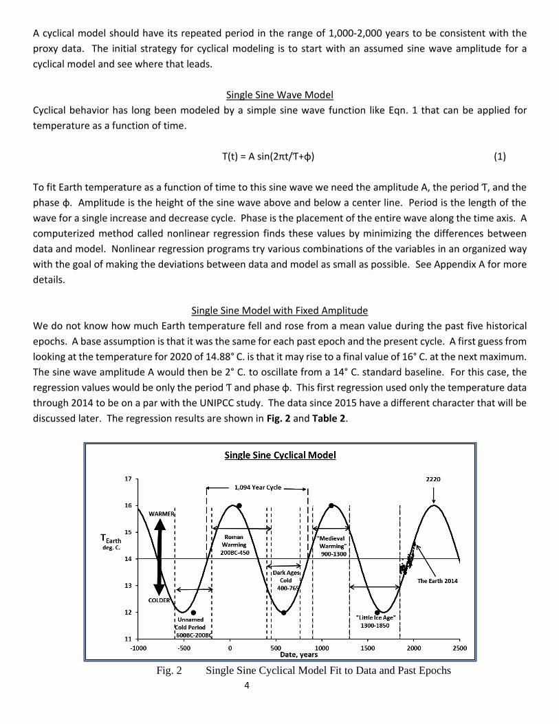
If you look closely at the measured temperatures compared to this single sine wave curve in Fig. 3, it is apparent
that there is another cyclical variant present. The experienced eye of a nonlinear modeler notices that the data
in Fig. 3 exhibit an oscillation. It looks like another sine wave needs to be added to the first one. This regular
trend is a strong indication that even though the fit looks reasonable in Fig. 2, improvements to the model must
be made.
Fig. 3 Deviation of Earth Temperatures from the Single Sine Cyclical Model
This second sine wave would have been needed even if a constant wave amplitude had not been assumed for
the first fit. The oscillation is inherent in the temperature data.
Dual Sine Cyclical Model
When a second sine wave is added to the first, the nonlinear regression results are shown in Fig. 4. For this fit
all parameters for both sine waves were regression variables, the amplitudes, periods, and phases. A constant
primary wave amplitude was not assumed. Temperature data through 2020 were used for this fit to be able to
model all the data. Table 3 shows the parameters for this fit.

6
Fig. 4 Dual Sine Cyclical Model Fit to Data and Past Epochs
Table 3 Two Sine Cyclical Model Parameters
Two Sine Model Sine 1 Sine 2
Period, years 1009 76.3
Amplitude, deg C. 1.23 0.24
Phase, radians 176.4 111.8
This dual sine model predicts that the Earth’s temperature will increase only about another 0.42° C. which will
be achieved in about 180 years in the year 2200 with a maximum temperature then of about 15.3° C. Total
temperature increases since 1850 would be about 1.95° C. Note that the amplitude of the first sine wave was
found to be 1.23° C., not the 2° C. of the first regression. Also, the period of 1009 years is shorter though not
greatly different from the 1094 years found by the Single Sine Cyclical Model. Fig. 5 shows that Earth
temperature oscillations agree well with the Dual Sine Cyclical Model. The second sine wave oscillation has a
period of 76 years according to this fit. Note that the 2015 to 2020 data fit the curve reasonably well.
Fig. 5 Deviation of Earth Temperatures from the Dual Sine Cyclical Model
7
To include the 2015-2020 data in this model, the weights for these years were increased to five compared to
one for the rest of the data points. This was done because these data diverge so much from past years, and a
fit including them was necessary. Appendix B shows the relatively large temperature increase following the
1998-2014 hiatus versus the much smaller increase after the 1940-1980 similar hiatus.
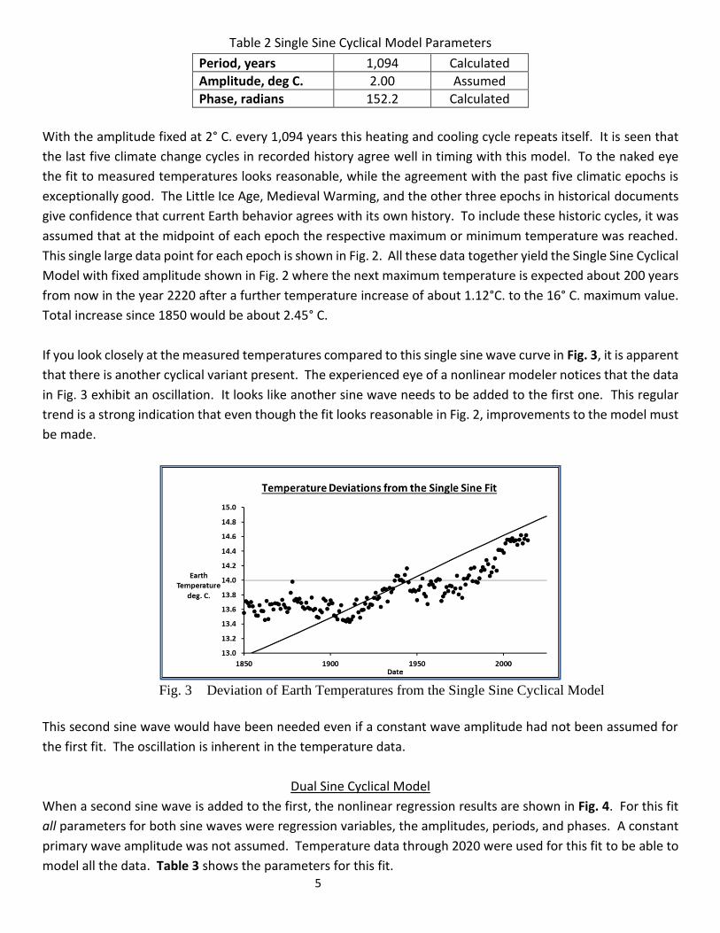
A plot like Fig. 5 with the time axis lengthened to the point of predicted maximum temperatures for the Dual
Sine Model is in Fig. 6. It shows that the maximum temperature will happen about 2200. Note also that the
Dual Sine Model predicts that temperatures should fall about 0.20° C. during the next 30 years to continue the
secondary cycle found in the Earth temperature data. This is a bold prediction.
Fig. 6 Predicted Maximum Temperatures of the Dual Sine Cyclical Model
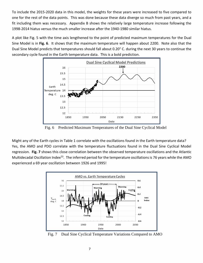
Might any of the Earth cycles in Table 1 correlate with the oscillations found in the Earth temperature data?
Yes, the AMO and PDO correlate with the temperature fluctuations found in the Dual Sine Cyclical Model
regression. Fig. 7 shows this close correlation between the observed temperature oscillations and the Atlantic
Multidecadal Oscillation Index23. The inferred period for the temperature oscillations is 76 years while the AMO
experienced a 69 year oscillation between 1926 and 1995!
Fig. 7 Dual Sine Cyclical Temperature Variations Compared to AMO
8
Not only does the AMO have essentially the same period, but it is also in close sync with the increases and
decreases of the temperature fluctuations. When the Earth temperature fluctuations are increasing, so is the
AMO. And, when the Earth temperature fluctuations are decreasing, so is the AMO. From Fig. 7 the expectation
would be that there would be another decrease of the AMO index during the next 20 to 30 years leading to
some cooling. The AMO might be causally related to the Earth’s secondary temperature fluctuations.
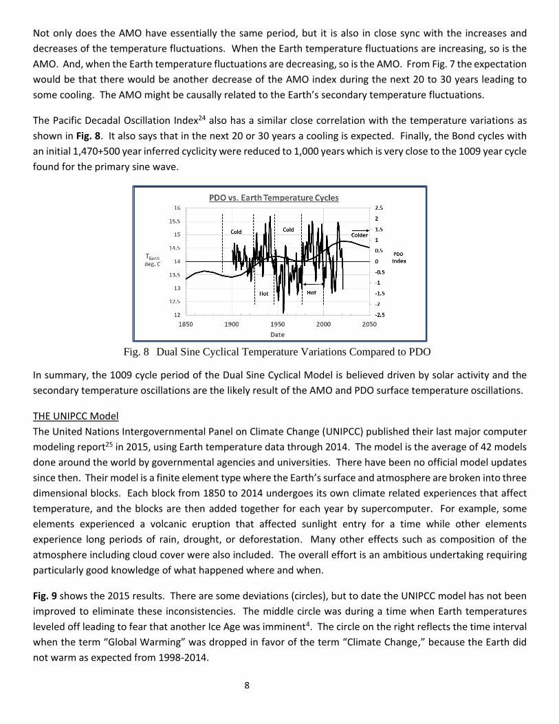
The Pacific Decadal Oscillation Index24 also has a similar close correlation with the temperature variations as
shown in Fig. 8. It also says that in the next 20 or 30 years a cooling is expected. Finally, the Bond cycles with
an initial 1,470+500 year inferred cyclicity were reduced to 1,000 years which is very close to the 1009 year cycle
found for the primary sine wave.
Fig. 8 Dual Sine Cyclical Temperature Variations Compared to PDO
In summary, the 1009 cycle period of the Dual Sine Cyclical Model is believed driven by solar activity and the
secondary temperature oscillations are the likely result of the AMO and PDO surface temperature oscillations.
THE UNIPCC Model
The United Nations Intergovernmental Panel on Climate Change (UNIPCC) published their last major computer
modeling report25 in 2015, using Earth temperature data through 2014. The model is the average of 42 models
done around the world by governmental agencies and universities. There have been no official model updates
since then. Their model is a finite element type where the Earth’s surface and atmosphere are broken into three
dimensional blocks. Each block from 1850 to 2014 undergoes its own climate related experiences that affect
temperature, and the blocks are then added together for each year by supercomputer. For example, some
elements experienced a volcanic eruption that affected sunlight entry for a time while other elements
experience long periods of rain, drought, or deforestation. Many other effects such as composition of the
atmosphere including cloud cover were also included. The overall effort is an ambitious undertaking requiring
particularly good knowledge of what happened where and when.
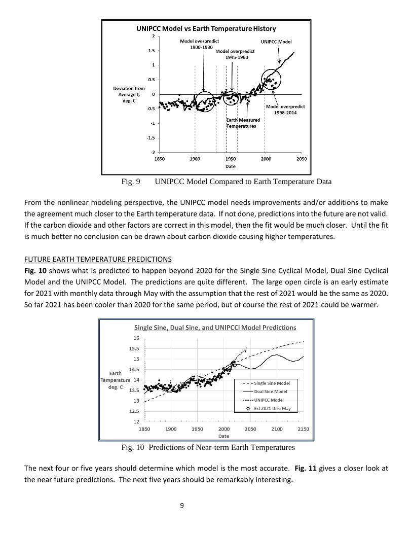
Fig. 9 shows the 2015 results. There are some deviations (circles), but to date the UNIPCC model has not been
improved to eliminate these inconsistencies. The middle circle was during a time when Earth temperatures
leveled off leading to fear that another Ice Age was imminent4. The circle on the right reflects the time interval
when the term “Global Warming” was dropped in favor of the term “Climate Change,” because the Earth did
not warm as expected from 1998-2014.
9
Fig. 9 UNIPCC Model Compared to Earth Temperature Data
From the nonlinear modeling perspective, the UNIPCC model needs improvements and/or additions to make
the agreement much closer to the Earth temperature data. If not done, predictions into the future are not valid.
If the carbon dioxide and other factors are correct in this model, then the fit would be much closer. Until the fit
is much better no conclusion can be drawn about carbon dioxide causing higher temperatures.
FUTURE EARTH TEMPERATURE PREDICTIONS
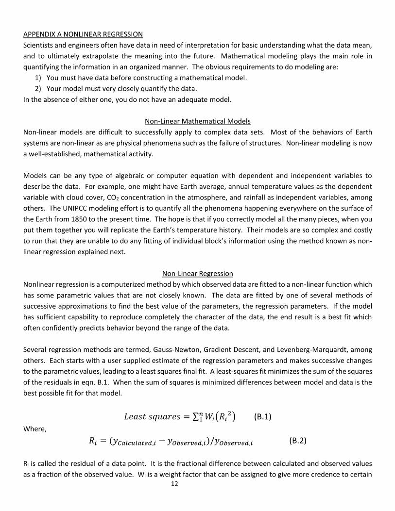
Fig. 10 shows what is predicted to happen beyond 2020 for the Single Sine Cyclical Model, Dual Sine Cyclical
Model and the UNIPCC Model. The predictions are quite different. The large open circle is an early estimate
for 2021 with monthly data through May with the assumption that the rest of 2021 would be the same as 2020.
So far 2021 has been cooler than 2020 for the same period, but of course the rest of 2021 could be warmer.
Fig. 10 Predictions of Near-term Earth Temperatures
The next four or five years should determine which model is the most accurate. Fig. 11 gives a closer look at
the near future predictions. The next five years should be remarkably interesting.

10
Fig. 11 Predictions of Near-term Earth Temperatures – Closer View
CONCLUSIONS
The information presented in this paper has led the author to conclude the following:
1. The increasing temperature of the Earth since 1850 is part of the natural temperature cycle that has
occurred on Earth for at least the last 3,000 years. The Dual Sine Cyclical Model fully explains both the
distant past and current temperatures. Maximum Earth temperature should be reached in about 180-
200 years.
2. Solid evidence for the reality of the Dual Sine Cyclical Model for Earth temperatures comes from analysis
of measured temperature data since 1850, the last five historical temperature cycles reported in history,
and the observation that the small temperature fluctuations found in the temperature data are likely
related to natural events known as the Atlantic Multidecadal Oscillation and Pacific Decadal Oscillation.
3. Changes ahead during the next two centuries will require adaptations including population migration to
cooler parts of the Earth and use of our energy sources to keep especially warm areas livable.
4. The next 4 or 5 years of annual Earth temperatures will determine which climate model predicts the
future best – The Single Sine Model, The Dual Sine Model or the United Nations Intergovernmental Panel
on Climate Change. The Single Sine and Dual Sine Cyclical Model have the best chance to bracket the
new data based on their scientific and historical backgrounds.
NOMENCLATURE
A = amplitude of a sine wave, deg. C.
AMO = Atlantic Multidecadal Oscillation – systematic movement of water from the Caribbean to Labrador
Least Squares = sum of the squared Ri values at the regression end, dimensionless
φ = phase of sine wave, radians – movement on the time axis
Ri = residual of a data point, dimensionless (Eqn. B.2)
t = time, years
Ƭ = period of a sine wave, years
Wi = weight factor, usually 1
YCalculated,I = calculated value of a temperature, deg. C.

11
YObserved,I = measured value of a temperature, deg. C.
REFERENCES
1) ‘We’re doomed’: Mayer Hillman on the climate reality no one else will dare mention “We’re doomed”,
www.theguardian.com, April 26,2018.
2) What is the greenhouse effect? – Climate Change: Vital Signs of the Planet (nasa.gov)
3) Singer, S. Fred, and Avery, Dennis T., Unstoppable Global Warming – Every 1,500 Years, Rowland &
Littlefield Publishers, Inc., 2006.
4) History of Earth's temperature since 1880 | NOAA Climate.gov
5) Time Magazine, Another Ice Age? April 14, 1974, pp. 86. 6) Los Angeles Times, Detailed look at the global warming ‘hiatus’ again confirms that humans are
changing the climate, May 3, 2017. 7) A buoy-only sea surface temperature record | Climate Etc. (judithcurry.com), November 22, 2015
8) Milankovitch (Orbital) Cycles and Their Role in Earth's Climate – Climate Change: Vital Signs of the Planet
(nasa.gov)
9) Strokosz, M. A., and H. L. Bryden, Observing the Atlantic Meridional Overturning Circulation yields a
decade of inevitable surprises, Science vol 348, issue 6241, June 19, 2015.
10) SVS: Historical Atlantic Multidecadal Oscillation (AMO) (nasa.gov)
11) Bond, Gerard, et. al., A Persuasive Millennial-Scale Cycle in North Atlantic Holocene and Glacial Climates,
Science, Vol 278, November 144, 1997,1257-1266.
12) Obrochta, Stephen P., et. al., Climate variability and ice-sheet dynamics during the last three glaciations,
Earth and Planetary Letters, vol 406, 2014, 198-212.
13) Mantua, Nathan J., Steven R. Hare, The Pacific Decadal Oscillation, Journal of Oceanography, Vol. 58, August 16, 2001, 35-44
14) Exploring AMOC’s impact on global and regional climate with Rong Zhang – Geophysical Fluid Dynamics
Laboratory (noaa.gov)
15) Atlantic Multi-decadal Oscillation (AMO) | NCAR - Climate Data Guide (ucar.edu) 16) Singer, S. Fred, and Avery, Dennis T., Unstoppable Global Warming – Every 1,500 Years, Rowland &
Littlefield Publishers, Inc., 2006. 17) Lorius, C. et. al., A 150,000 Year Climate History from Ice Cores, Nature 316 1985, pp. 591-596.
18) Singer, S. Fred, and Avery, Dennis T., Unstoppable Global Warming – Every 1500 Years, Rowland & Littlefield Publishers, Inc., 2006, pp. 21-34.
19) Singer, S. Fred, and Avery, Dennis T., Unstoppable Global Warming – Every 1500 Years, Rowland &
Littlefield Publishers, Inc., 2006, pp. 191-199
20) Braun, Holger et. al., Possible solar origin of the 1,470 year glacial climate cycle demonstrated in a
coupled model, Nature, 438,7065, 208-211.
21) Lamb, H. H., Climate, History and the Modern World, Psychology Press, 1995, 187-189
22) Duell, Mark, Thrills of the frost fair: Fascinating paintings and memorabilia show how Londoners celebrated
when the River Thames froze over, Daily Mail, December 25, 2013.
23) Download Climate Timeseries: AMO SST: NOAA Physical Sciences Laboratory
24) https://psl.noaa.gov/data/correlation/amon.us.long.data
25) https://unfccc.int/topics/science/workstreams/cooperation-with-the-ipcc/the-fifth-assessment-report-
of-of-the-ipcc
12
APPENDIX A NONLINEAR REGRESSION
Scientists and engineers often have data in need of interpretation for basic understanding what the data mean,
and to ultimately extrapolate the meaning into the future. Mathematical modeling plays the main role in
quantifying the information in an organized manner. The obvious requirements to do modeling are:
1) You must have data before constructing a mathematical model.
2) Your model must very closely quantify the data.
In the absence of either one, you do not have an adequate model.
Non-Linear Mathematical Models
Non-linear models are difficult to successfully apply to complex data sets. Most of the behaviors of Earth
systems are non-linear as are physical phenomena such as the failure of structures. Non-linear modeling is now
a well-established, mathematical activity.
Models can be any type of algebraic or computer equation with dependent and independent variables to
describe the data. For example, one might have Earth average, annual temperature values as the dependent
variable with cloud cover, CO2 concentration in the atmosphere, and rainfall as independent variables, among
others. The UNIPCC modeling effort is to quantify all the phenomena happening everywhere on the surface of
the Earth from 1850 to the present time. The hope is that if you correctly model all the many pieces, when you
put them together you will replicate the Earth’s temperature history. Their models are so complex and costly
to run that they are unable to do any fitting of individual block’s information using the method known as non-
linear regression explained next.
Non-Linear Regression
Nonlinear regression is a computerized method by which observed data are fitted to a non-linear function which
has some parametric values that are not closely known. The data are fitted by one of several methods of
successive approximations to find the best value of the parameters, the regression parameters. If the model
has sufficient capability to reproduce completely the character of the data, the end result is a best fit which
often confidently predicts behavior beyond the range of the data.
Several regression methods are termed, Gauss-Newton, Gradient Descent, and Levenberg-Marquardt, among
others. Each starts with a user supplied estimate of the regression parameters and makes successive changes
to the parametric values, leading to a least squares final fit. A least-squares fit minimizes the sum of the squares
of the residuals in eqn. B.1. When the sum of squares is minimized differences between model and data is the
best possible fit for that model.
𝐿𝑒𝑎𝑠𝑡 𝑠𝑞𝑢𝑎𝑟𝑒𝑠 = ∑ 𝑊𝑖(𝑅𝑖2)𝑛
1 (B.1)
Where,
𝑅𝑖 = (𝑦𝐶𝑎𝑙𝑐𝑢𝑙𝑎𝑡𝑒𝑑,𝑖 − 𝑦𝑂𝑏𝑠𝑒𝑟𝑣𝑒𝑑,𝑖)/𝑦𝑂𝑏𝑠𝑒𝑟𝑣𝑒𝑑,𝑖 (B.2)
Ri is called the residual of a data point. It is the fractional difference between calculated and observed values
as a fraction of the observed value. Wi is a weight factor that can be assigned to give more credence to certain
13
points. For example, more accurate values based on improved measurement methods. The residuals are
squared in the sum of squares to be minimized by nonlinear regression so that positive and negative residuals
are treated equally. If not squared, a large negative and a large positive residual would merely cancel each other
out giving a misleading result. With most data being measured in some way, there are always measurement
errors termed random errors. Measuring equipment or personal observations of some event always introduced
some uncertainty. The non-linear regression program used in this work was the Solver in MS Excel 365.
APPENDIX B NOAA TEMPERATURE REPORTS
Earth Temperature Response after Plateaus
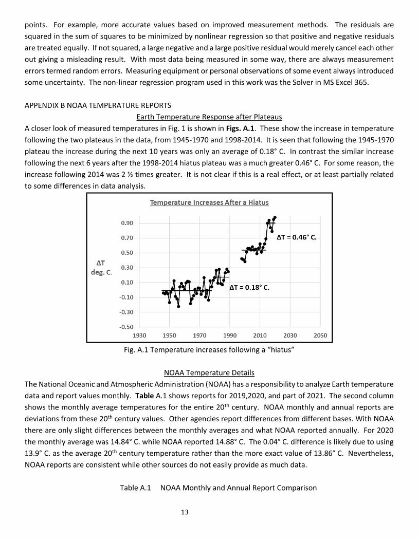
A closer look of measured temperatures in Fig. 1 is shown in Figs. A.1. These show the increase in temperature
following the two plateaus in the data, from 1945-1970 and 1998-2014. It is seen that following the 1945-1970
plateau the increase during the next 10 years was only an average of 0.18° C. In contrast the similar increase
following the next 6 years after the 1998-2014 hiatus plateau was a much greater 0.46° C. For some reason, the
increase following 2014 was 2 ½ times greater. It is not clear if this is a real effect, or at least partially related
to some differences in data analysis.
Fig. A.1 Temperature increases following a “hiatus”
NOAA Temperature Details
The National Oceanic and Atmospheric Administration (NOAA) has a responsibility to analyze Earth temperature
data and report values monthly. Table A.1 shows reports for 2019,2020, and part of 2021. The second column
shows the monthly average temperatures for the entire 20th century. NOAA monthly and annual reports are
deviations from these 20th century values. Other agencies report differences from different bases. With NOAA
there are only slight differences between the monthly averages and what NOAA reported annually. For 2020
the monthly average was 14.84° C. while NOAA reported 14.88° C. The 0.04° C. difference is likely due to using
13.9° C. as the average 20th century temperature rather than the more exact value of 13.86° C. Nevertheless,
NOAA reports are consistent while other sources do not easily provide as much data.
Table A.1 NOAA Monthly and Annual Report Comparison
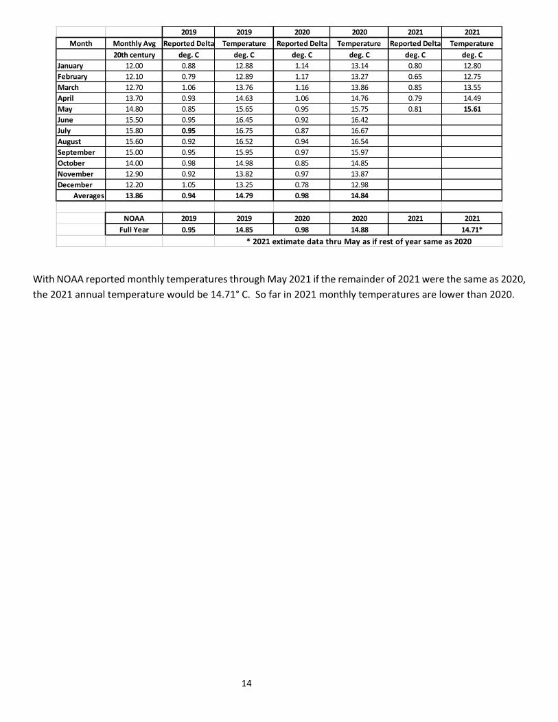
14
With NOAA reported monthly temperatures through May 2021 if the remainder of 2021 were the same as 2020,
the 2021 annual temperature would be 14.71° C. So far in 2021 monthly temperatures are lower than 2020.
2019 2019 2020 2020 2021 2021
Month Monthly Avg Reported Delta Temperature Reported Delta Temperature Reported Delta Temperature
20th century deg. C deg. C deg. C deg. C deg. C deg. C
January 12.00 0.88 12.88 1.14 13.14 0.80 12.80
February 12.10 0.79 12.89 1.17 13.27 0.65 12.75
March 12.70 1.06 13.76 1.16 13.86 0.85 13.55
April 13.70 0.93 14.63 1.06 14.76 0.79 14.49
May 14.80 0.85 15.65 0.95 15.75 0.81 15.61
June 15.50 0.95 16.45 0.92 16.42
July 15.80 0.95 16.75 0.87 16.67
August 15.60 0.92 16.52 0.94 16.54
September 15.00 0.95 15.95 0.97 15.97
October 14.00 0.98 14.98 0.85 14.85
November 12.90 0.92 13.82 0.97 13.87
December 12.20 1.05 13.25 0.78 12.98
Averages 13.86 0.94 14.79 0.98 14.84
NOAA 2019 2019 2020 2020 2021 2021
Full Year 0.95 14.85 0.98 14.88 14.71*
* 2021 extimate data thru May as if rest of year same as 2020