the day that wti died: asset prices and firm production

The Day that WTI Died:

Asset Prices and Firm Production Decisions

Erik P. Gilje∗ Robert Ready† Nick Roussanov‡ Jérôme P. Taillard§

November 11, 2020

Abstract

On April 20, 2020 the flagship North American benchmark price for crude oil, WestTexas Intermediate (WTI) for delivery in Cushing, OK, went negative for the first timein history, settling at -$37/bbl. We document that this event had a widespread effecton physical purchase contracts throughout the United States, despite ample storagecapacity at many locations. We show that firms with crude purchase contracts indexedto WTI shut-in production after this event at greater rates than those that did not.The difference in behavior is strongest among high productivity wells and occurs despitean overall improvement in pricing and crude market fundamentals after the April 20thevent. Our evidence suggests that asset prices have important implications for the realactions of firms due to their importance as price setting mechanisms in contracting.

∗The Wharton School, University of Pennsylvania, 3620 Locust Walk Suite, 2400, Philadelphia, PA 19104.Email: [email protected]†Lundquist College of Business, 382 Lillis Hall, 1208 University of Oregon, Eugene, OR 97403. Email:

[email protected]‡The Wharton School, University of Pennsylvania, 3620 Locust Walk Suite, 2400, Philadelphia, PA 19104.

Email: [email protected]§Babson College, 323 Tomasso Hall, Babson Park, MA 02457. Email: [email protected]

1

1 Introduction

The feedback effect between financial market asset prices and real decisions by firms has

been a central focus of the finance and economics literature (Hayek (1945) and Bond et al.

(2012)). Confidence in the role of market prices in serving as aggregators of information

has led to widespread adoption by firms of pricing mechanisms based on market-based ben-

chmarks for sales contracts, debt contracts, compensation contracts, and other inter firm

contractual arrangements (Duffie and Stein (2015)). While benchmarking to market prices

address a number of frictions (e.g. information asymmetry), it also potentially exposes firms

to additional risks. On April 20, 2020, for the first time in history, the flagship North Ameri-

can benchmark contract price for crude oil, West Texas Intermediate for delivery in Cushing,

Oklahoma, went negative settling at -$37/bbl. Because most crude purchase contracts in

the United States are indexed to WTI, millions of barrels of crude in America were sold for

-$37 on April 20, 2020, despite ample storage in many locations across the United States.

We trace out the effect of this event on firm production, and provide novel evidence on a

previously under appreciated dimension through which asset prices, via a benchmark pricing

channel, can affect the real decisions of firms.

The most liquid and actively traded crude oil contract in the world is the NYMEX

West Texas Intermediate (WTI) contract traded on the Chicago Mercantile Exchange. This

contract specifies a certain crude oil quality, to be delivered at a certain location (Cushing,

Oklahoma) at a certain point in time. Both financial traders and physical traders can engage

in trading on the exchange. The commonly quoted price of crude oil by media outlets, and

used in academic research, is the “front month” or the nearest month available for delivery

at Cushing, OK among all futures contracts on WTI. Due to the high degree of liquidity

in this front month contract, the interconnectedness of the United States energy complex

with Cushing via pipeline, and the fact that Cushing is the largest commercial crude storage

site in the United States, many physical buyers and sellers of oil have their crude sales

agreements indexed to the price of oil in Cushing (WTI prices). Even if transactions occur

geographically far from Cushing or are for different grades of crude, transactions benefit from

2

the price informativeness and price discovery at Cushing. However, this convention can also

set the stage for crude producers being tethered to pricing that could get dislocated were

there ever to be dislocations in the front month WTI prices due to physical constraints or

deliverability issues at Cushing.

On April 20, 2020, the May contract was the front month, and any traders that had not

exited their positions by settlement on April 21, 2020 would need to take physical delivery

of the crude they had in futures positions that had not been closed. Delivery at Cushing

requires either a volume allocation on a pipeline in or out of Cushing or a physical terminal

at Cushing, there is not flex capacity or pickup available via waterborne delivery or truck.

Therefore Cushing is a closed system with a fixed amount of storage and pipeline capacity.

As sellers began to outnumber buyers on the evening of April 19, 2020 the price of crude fell,

the selling accelerated the next morning, culminating in prices going negative for the first

time around 1PM on April 20, 2020 (see Figure 1 and Figure 2). Prices remained negative

and the daily contract settlement at 2:30 was for -$37/bbl. This settlement price, regardless

of the trading volume at the time, is what was important for index and benchmark pricing

across the U.S. crude oil complex. Even though prices remained below -$10/bbl for only 5

hours on April 20th, 80 crude grades at locations across the United States transacted at an

average of -$44/bbl even at locations that had ample storage capacity as well as waterborne

flex storage capacity.

Our contribution is to study how this event reverberated across the real decisions made

by firms. This setting provides a unique opportunity to explore the importance of how asset

prices, via benchmarks, affect the real decisions of firms. Specifically, while crude oil funda-

mentals were undoubtedly challenging due to the COVID-19 pandemic we provide evidence

that the negative price spike in WTI was consistent with concerns regarding deliverability and

storage issues at Cushing, and not reflective of broader fundamental prices at other locations

that were indexed to Cushing. Therefore, this setting provides an attractive way to estimate

how the functioning of asset markets that firms reference for contractual arrangements are

important for real production decisions.

Our main results compare production decisions made for oil wells indexed to WTI to a

3

control set of wells that are not benchmarked to WTI. Given our high frequency data, these

comparisons are made at several points in time around the event and allows us to rule out

several confounding explanations. Specifically our counterfactual wells are located in Canada

and California, both of which have different pricing mechanisms underpinning their crude

market. Our main outcome measure is whether firms throttle back production by shutting in

production from wells. Namely, we look at whether a well producing in March of 2020 is shut-

in in April 2020, May 2020, or June 2020. Our data allow us to observe firm-level production

decisions at the well-firm-month level and our tests rely on data from 109,680 individual

wells. We initially focus on oil wells producing in North Dakota, which are indexed to WTI

as these wells have similar characteristics to non-oil sands wells in Canada, and also satisfy

parallel trends with wells in California. We find that in the Spring of 2020 the proportion

of North Dakota wells that are shut-in is 17% higher than comparable wells in Canada (not

directly indexed to WTI) and 43% higher than comparable wells in California (where prices

did not go negative on April 20th).

There are arguably any number of differences across geographies and well types that

could drive this result. It could be that wells in North Dakota are less profitable to operate

than wells in other areas, or have some other characteristic that is driving this behavior.

We conduct all of our main analysis controlling for well productivity, which goes some way

towards allaying such concerns. We also document parallel trends between North Dakota

(high WTI exposure) and the counterfactual comparison groups. However, our strongest

evidence on the importance of the April 20th event comes from the inter-temporal response

of North Dakota producers that we observe. On April 1, 2020, prior to the negative price

spike, spot prices in North Dakota were $8.98/BBL. After the negative price spike in April,

on May 1, 2020 spot prices in North Dakota were $22.28. This pricing would suggest that

the May pricing environment was better than April, yet we see substantially more shut-ins

occur in May in North Dakota, particularly of high productivity wells. In fact April shut-in

activity mimics the shut-in activity in Canada quite closely. It is in fact the May shut-in

activity, when pricing has improved dramatically - but after the negative price spike - that

we observe the bifurcation in shut-in behavior across North Dakota (high WTI exposure)

4

relative to Canada (low WTI exposure).

We also conduct a series of tests focused on higher frequency, daily production measures

at the state level from pipeline flow (a proxy for production) data. If producers are concerned

about potential negative price spikes around the contract expiration of crude oil contracts

in Cushing, and the associated dislocations, there are a series of predictions one might have

related to daily production data. First, one might expect that on May 1, the first day a

producer’s calendar month average price might be affected by a negative WTI price spike in

May, when the front month contract expires and rolls to a new month on May 19th, that

production would be shut-in. We observe a 4 standard deviation reduction in our production

proxies from April 30 to May 1. Second, one might expect that after the contract expiration

in May (for June delivery) that producers may start re-opening wells if a negative price spike

is not observed on the contract expiration/roll. This is in fact what we observe, the day

after contract expiration (May 20th), our production proxies begin to increase, and increase

through the end of the month. Put together, these pieces of evidence are consistent with

the negative price shock and contract roll risk at Cushing having a real effect on production

decisions.

Our results relate to several strands of literature. Most notably we relate to the literature

in finance and economics that focuses on the interaction between financial markets and the

real decisions of firms (for a summary see Bond et al. (2012)). This literature goes back

at least to Hayek (1945) and argues that secondary market prices for assets are important

sources of information. This line of thought is clearly one reason why firms may want to

contract around these prices, as in our setting. The focus of this literature, both theoretical

and empirical, is largely around the informativeness of equity prices. That is equity prices can

1) help managers decide when to invest and what to invest in (Chen et al. (2007), Foucault

and Fresard (2012), Barro (1990)) 2) help managers deciede whether to undertake merger

decisions (Luo (2005) and Edmans et al. (2012)) 3) help customers or employees decide which

firm to work for. There has been less of a focus in the literature in terms of how contracting

around market prices occurs, and when contract prices are affected by dislocations and/or

limits to arbitrage what are the potential ramifications in terms of real effects.

5

Our results also contribute to the literature on the financialization of commodity markets

(Cheng and Xiong (2014)). For example, exchange traded funds own substantial portions of

futures contracts, positions that have both evolved over time and are subject to regulatory

scrutiny. While it is still unclear to what extent the events of April 20, 2020 relate directly

to financialization versus fundamental constraints and limits to arbitrage in Cushing, our

evidence points to how any potential distortion in prices caused by financialization could have

important implications for how real producers interact, due to the tethering of real/physical

sales prices to financialized assets.

2 Institutional Detail and Data

In this section we provide some background on crude oil futures contracts, crude oil

purchase contracts, and pricing mechanisms.

Firms pay crude oil purchasers to purchase oil from the wellhead. Crude purchasers

typically drive up to a well with a truck owned by the purchaser and fills the truck up from

tanks on the well location. The purchaser then trucks this oil to a pipeline or terminal

and then the crude oil is brought to market and processed at a refinery. In essence crude is

transacted at tens of thousands of locations every day. The problem of setting the transacting

price is laid out by Duffie and Stein (2015), without an independent benchmark price to settle

the transaction, the buyer and seller could easily disagree on what the fair market price is

for crude at the well site, hence there are a number of factors that drive a pricing mechanism

based on a tradable index. As Duffie and Stein (2015) layout, market particpants that use a

benchmark in their transaction will “reap the information benefits of a benchmark...including

lower search costs, higher market participation, better matching efficiency, and lower moral

hazard in delegated execution. In order to obtain these benefits, market participants or their

agents will often choose to substitute their “best-fit-for purpose” trade with a benchmark

trade. The flagship, most liquid benchmark for crude oil in North America is given by the

West Texas Intermediate (WTI) for delivery in Cushing, OK. Hence pricing mechanisms

6

throughout the United States are derived from this index.

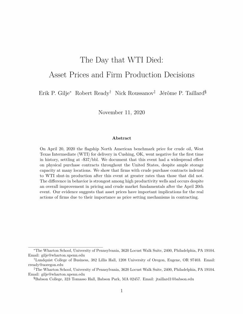
It is important to note that crude oil purchase agreements are not based on the price

of crude on a given day, but rather, on the calendar month average (CMA) of index prices.

As reported in Figure 3, this means that oil sold early in the month will be subject to

price fluctuations that occur later in the month. Moreover, this means that if crude indices

were to settle at a negative value on a given day, this negative number is incorporated in

the calendar month average, effectively rendering all crude sold on that given day as being

transacted at the negative price. The nature of this contract arrangement is supported by the

letter Harold Hamm, CEO of Continental Resources wrote to the CFTC stating the events

of April 20th “materially impacts the Calendar Month Average (CMA) pricing of physical

crude,” as presented in Figure 3. Figure 4 reports the Calendar month postings for crude

grades purchased by the refiner Phillips 66. As can be seen, crude grades at locations far

from Cushing, including Texas (WT Inter), New Mexico (NM Inter), and Louisiana (LLS

Onshore), were marked at negative values on April 20th. These represent real prices that

were included in Calendar Month Averages.

We collect data from every major crude oil purchaser in the United States and their posted

contract prices. In total we collect data on 101 crude grade-location pairs. In Figure 5A,

we report the prices of a sampling of these grades overlaid on a pipeline map of the United

States. As can be seen crude grades from Texas to Michigan were transacted at negative

values on April 20th. Perhaps most interestingly, even water borne grades from the Middle

East delivered to the U.S. Gulf Coast went negative on this day. According to the Oxford

Instititute for Energy Studies, in 2009, Saudi Arabia, Kuwait, and Iraq all shifted to a pricing

mechanism based on the Argus Sour Crude Index which is a weighted average of crude grade

prices on the United States Gulf Coast (ASCI). Because Argus sets the Chicago Mercantile

Exchange’s NYMEX WTI prices as the underlying fixed price for ASCI even these Middle

Eastern grades were marketed to a negative price, in this instance -$26.63. Unlike Cushing,

water borne grades are not subject to fixed capacity constraints, as barges and tankers can be

used as flex capacity. We will provide additional direct evidence later in this paper, but the

fact that crude grades with water borne access go negative on this particular day, would seem

7

to be inconsistent with fundamentals outside of Cushing where water borne access should

allow for flex capacity. Meaning, the events occurring in Cushing OK led to a contagion

effect with a generalized dislocation of crude prices on that day for most of North America.

Figure 6 plots a histogram of posted prices from Crude Oil purchasers in the U.S. on

April 20, 2020. All crude grades in the U.S., except for California, went negative. Why

might crude grades in California be positive? As can be seen in Figure 5A these grades

are on a distinct pipeline network, and therefore the price setting mechanisms and linkages

with Cushing are distinct from the rest of the United States. A central issue we will try to

assess throughout our paper is to what extent are we identifying a “low price effect” versus

a “WTI negative price shock” effect. Our tests are designed to help distinguish between the

two effects. Or put differently, in our counterfactual comparison sets, both California and

Canada have pricing mechanisms that result in low prices, but concurrently insulated them

from the negative WTI prices of April 20, 2020.

Canadian crude is connected to the United States via pipeline. However, these crude

grades operate off of distinct pricing mechanisms from most U.S. crude grades. There is an

exchange and storage hub in Edmonton, which allows for price movements distinct from WTI

which insulate these grades at least to some extent from physical limits to arbitrage issues at

Cushing. Because these grades are connected via a pipeline network to Cushing we do not

view Canadian crude as insulated as California crude from physical dislocations at Cushing.

2.1 Well Data

Our empirical design requires us to construct a dataset of individual wells and production

for the United States and Canada for 2019 and 2020. We rely on two different data sources.

For all United States data we rely on DrillingInfo, which provides detailed well level data

by month, by producer, with detailed geographic location data for most jurisdictions in

the United States. In our study we predominantly focus on North Dakota and California

producers. Our Canadian data is downloaded from a website maintained by the province

of Alberta, and is also at the well-level, by producer, monthly. In total we have 109,680

wells across the United States and Canada in our study. We focus on wells that are arguably

8

similar to one another, in particular Canada has substantial production from oil sands, which

is a distinct production technology, therefore we limit our Canadian data to non-oil sands

wells that produce a crude grade similar to WTI. We report data on our sample in Table 1.

2.2 Price Data

Data on daily benchmark prices is obtained from Bloomberg, and intra day price and volume

data is obtained from the CME. We also hand collect posted prices from crude purchasers off

of their websites. We report pricing for each of the key geographies we discuss in this paper

in Table 1.

2.3 Fundamentals of Crude Oil Supply and Demand

The Spring of 2020 saw an unprecedented crude oil demand shock. It is estimated that

demand destruction reached approximately 20 million barrels/day, or roughly 20% of all crude

oil being consumed prior to COVID-19. A key challenge to our identification is assessing to

what extent the behavior we are observing is due to this fundamental macro shock relative to

the WTI benchmark risk we are attempting to measure. To explore how these factors could

affect our empirical tests we estimate a number of counterfactuals across firms and over time.

But we begin by assessing to what extent the fundamental physical dynamics at Cushing are

affecting the WTI benchmark, relative to the other benchmarks in our counterfactuals. A key

leading indicator for crude oil demand is refinery utilization. In the United States these data

are reported every week and broken out by region. We report refinery utilization by region

in Figure 5B. As can be seen, with the onset of COVID-19 lockdowns refinery utilization

dropped dramatically, with the biggest drop occurring on the West Coast. This is consistent

with one of the most aggressive lockdown measures occurring in California. Yet, despite a

stronger drop in refinery utilization than any other area, the U.S. west coast was the only

region in the United States not to suffer from a negative price spike on April 20, 2020.

In addition to refinery utilization, storage is another key indicator driving oil markets and

prices. If supply exceeds demand, storage utilization goes up, which often is associated with

9

oil price declines. If demand exceeds supply, there are storage draws, and conversely oil prices

typically increase. We plot in Figure 5C storage utilization across three areas of the United

States: (1) West Coast (California crude market), (2) Central United States connected to

Cushing via pipeline, and (3) storage utilization in Cushing itself. This figure brings to light

the dynamics at play on April 20, 2020, a dramatic rise in storage utilization at Cushing

over one month, going from 50% to 85%. In fact, this represented the biggest one month rise

in storage (in percentage terms) on record, and represented a 5 standard deviation move in

storage utilization. However, the data outside of Cushing are noteworthy also. In markets

outside of Cushing but connected to it via pipeline, storage levels remain subdued with

utilization in the 70% range, while storage utilization on the West Coast remained elevated

throughout the period.

The data presented in these two Figures outlining the fundamentals of crude at these

different locations are consistent with several observations. First, the West Coast was the

most fundamentally constrained of any crude oil market, it had the lowest persistent refinery

utilization and the highest storage utilization, yet did not witness negative pricing for crude.

By late April, the Midwest refinery utilization had already bottomed and was improving,

this Midwest market is the key market for North Dakota and Canadian crude. Lastly, as

Figure 5C shows, the main storage issue was in Cushing, not in connected markets, while

prices in Cushing could arguably go low, and even possibly negative, as storage hits its

maximum, storage was nowhere close to capacity outside of Cushing. So why couldn’t markets

outside of Cushing seamlessly absorb the excesses observed at Cushing? Crude movements

are constrained by pipeline capacities and allocations. However, we do see that between April

20th and May 31st, 12 million barrels of crude in Cushing were moved elsewhere and stored.

We also compile data on waterborne tanker rates in April from Bloomberg, and do not observe

any spike in tanker rates on April 20th. While April tanker rates are elevated, they are no

higher than tanker rates from the prior December. All of these data points point toward

Cushing being the primary location where physical deliverability issues would occur, and

result in prices arguably disconnected from fundamentals at all other U.S. locations where

crude is being transacted, as benchmark pricing at these locations is indexed to Cushing

10

(WTI) pricing.

3 Results

3.1 WTI Exposure and Shut-in Decisions

In this section we estimate how oil well shut-in decisions relate to having crude oil purchase

agreement indexed to WTI. We will compare production (shut-in) decisions in North Dakota,

to two areas that are less exposed to WTI, namely (1) Alberta in Canada and (2) California.

Each of these geographical areas serve as a “control” group with different attractive features.

Specifically, Alberta crude oil has the same end market as North Dakota, predominantly

refineries in the upper Midwest, and their oil feeds into the same pipeline network as North

Dakota crude. However, Alberta crude has a distinct pricing mechanism related to crude oil

prices set in Edmonton, Alberta. Excluding oil sands (heavy oil), the wells across Alberta

and North Dakota share similar characteristics. Alternatively, California is a distinct crude

market, with no crude oil pipeline connections to Cushing, OK or North Dakota. It has a

pricing mechanism distinct from WTI, but as pointed out in the prior figures has arguably

weaker underlying fundamentals than North Dakota crude due to the elevated storage levels

and lower refinery utilization compared to other areas. Figure 7 plots the crude oil price

movements in April and May of 2020 across these geographies. In effect, both Alberta and

California serve as proxies for “low WTI” exposure regions, while North Dakota serves as a

proxy for “high WTI” exposure regions.

We estimate the effect of WTI exposure by computing a regression form of difference-in-

differences:

Shutini,t = α+β1WTIExpi+β2Postt+β3Postt∗WTIExpi+lnProdi,t+StateFE+FirmFE+εi,t

The dependent variable of interest (Shutini,t) is an indicator variable 0 or 1 as to whether

a well has been shut-in in year t. The time period of our estimation is 2019 and 2020, we

specifically compare wells that are producing as of March in a given year, and then are shut-

11

in in April, May, or June of that year. For wells that are shut-in the indicator value is 1.

WTIExpi is equal to 1 if the oil well is in North Dakota, where it is indexed to WTI, and

is equal to 0 if the oil well is in Alberta or California where it would be subject to a distinct

pricing mechanism. Postt is equal to 1 if the time period is for 2020 shut-ins and is 0 if

the time period is for 2019 shut-ins. lnProdi,t is the natural logarithm of the production of

the well in March of year t for well i. The key coefficient of interest to assess whether WTI

exposure is associated with different shut-in behavior in 2020 around the negative WTI price

spike in April is the interaction coefficient, β3.

Table 2 reports the estimates of the regression specification above. The interaction coeffi-

cients are positive and statistically significant in each specification, indicating that production

was reduced, via shut-ins, in 2020 for high WTI exposure wells, relative to low WTI exposure

wells, when compared to the baseline shut-in behavior in 2019. Specifically, the coefficient in

(1) can be interpreted as wells in North Dakota, where WTI exposure is high, being shut-in

at a rate that is 17% higher, or half a standard deviation higher, relative to Alberta wells,

when compared to the same difference in the baseline period in 2019. The results are even

starker when comparing shut-in behavior of North Dakota to California, as the coefficient on

(3) is 0.43, or a 1.3 standard deviation increase in shut-in behavior. We also report these

results in a univariate manner in Figure 8 where we sort wells into bins based on productivity

and compare shut-in percentages in 2020 in Alberta and North Dakota. As one might ex-

pect, less productive/efficient wells are shut-in at a greater propensity, hence, justifying our

inclusion of this variable as a control. One can also see that, consistent with Table 2, shut-in

propensities are higher for each production bin in North Dakota relative to Alberta. We also

plot shut-in propensities for 2019 in Figure 9 to compare baseline behavior in Alberta and

North Dakota.

Although Table 2 reports results consistent with WTI exposure affecting the real pro-

duction decisions of firms, one may be concerned that wells in North Dakota are materially

different than other areas, and perhaps may trend differently for other reasons, for example

North Dakota wells could have an inherently higher cost structure. While we test for pa-

rallel trends explicitly later in the paper, our granular data allow us to compare month by

12

month shut-in decisions within North Dakota. Specifically, pricing had already deteriorated

substantially in North Dakota (as well as Canada) as of April 1. In North Dakota, crude oil

was marked at $8.98 on April 1 according to Bloomberg (see Table 1). This price is mate-

rially lower than the price on May 1, which was $22.28. If it is the case that producers are

shutting in due to low prices, we ought to observe more shut-ins in April relative to May in

North Dakota. However, if exposure to WTI benchmark negative price risk, and a potential

additional negative price spike in Cushing on the settlement date for the next period (May

19th) is driving firm behavior, one would expect more shut-ins in May.

We report month by month shut-in behavior in North Dakota in Panel A of Table 3,

and find that new shut-ins were 26.5% of all wells in North Dakota in May, as compared

to 16.4% of all wells in April, a difference that is statistically significant. We formalize

this month to month comparison by estimating another regression form of difference-in-

differences, comparing Alberta and North Dakota in Panel B of Table 3. We find that there

was no statistical differences in shut-in behavior across Alberta and North Dakota in April,

consistent with the low price environment in both places ($9.64 for April in North Dakota

and $9.02 in April in Alberta) driving similar behavior. Prices improve in May to $29.55 in

North Dakota and $26.31 in Alberta, however, many more wells are shut-in in North Dakota

relative to Alberta. This result is striking and consistent with WTI negative price exposure in

May 2020 having a material impact on the decision to shut-in by producers in North Dakota.

We report similar specifications in Panel C of Table 3 comparing North Dakota to Califor-

nia, and find the shut-ins concentrated in May relative to April in that comparison as well. In

addition to the regression specifications in Table 3, we provide univariate results comparing

shut-in behavior in April and May across Alberta and North Dakota in Figure 10A and 10B.

These results at the univariate level are consistent with what we see in the regression: when

prices are low, both North Dakota and Alberta oil wells are shut-in at similar propensities.

When prices recover, but just after North Dakota has experienced the WTI-related negative

oil price shock in April, we see shut-in propensities dramatically increase in May relative to

April, but only in North Dakota.

A basic identification assumption of the tests in Tables 2 and 3 is that in the absence of the

13

WTI negative price exposure, North Dakota would have exhibited similar shut-in behavior

to California and Alberta, or shut-in behavior that would have trended similarly. We test

for this directly in Table 4, where we estimate the same regression specification as Table 2,

but use a placebo time period for the post period. Instead of Post being the Spring of 2020

(April/May/June), we designate Post as the Summer of 2019, or more specifically, we look at

wells that were producing in June 2019 and shut-in in July 2019, August, 2019, or September

2019, all time periods prior to the onset of the COVID crisis. As can be seen from Table

4 results, coefficients on the interaction term of interest are not statistically significant, and

are at economic magnitudes that are approximately 3% only of the those reported in our

main results in Table 4. We also plot shut-in propensities throughout 2019 in Figure 11.

These seem to indicate that California and North Dakota trended similarly in their shut-in

behavior in 2019.

3.2 WTI Exposure and Contract Roll Risk

In this section we estimate how proxies for oil production change at the daily level, and

whether these changes are consistent with firms being concerned with negative oil prices at

Cushing. One of the factors associated with the negative oil price on April 20, 2020 was

the contract expiration of the contract for May delivery in Cushing. During these contract

expirations traders with financial positions in contracts must exit and find an offsetting

counterparty to close out the contract, or take physical delivery. As shown in Figure 2

Panels A and B, as contract expiration approaches, most volume moves to the contract for

the following month. We use high frequency pipeline flow data to assess whether firms are

adjusting production in a way that would be consistent with negative price spikes around

this contract “roll.” The data we have on pipeline flow is from natural gas, not oil, as oil

flow data is not publicly available. However, natural gas flow data can be a good indicator

of daily oil production changes because a portion of natural gas in the United States comes

from commingled production with oil. That is, if natural gas goes down from a region that

has commingled production, it is a direct indicator that oil production has also gone down.

14

We compare how this “associated” gas production compares to “dry” gas or unassociated

production by looking at production from states that have predominantly associated gas

(from oil wells) versus states that have predominantly dry gas (from natural gas wells).1

Our first empirical exercise explores whether firms adjust their oil production, and there-

fore their associated gas volumes , following their “new” exposure to negative WTI (bench-

mark) prices. The first such contract roll risk event occurs on May 19, 2020 (next settlement

date). The date firms first become exposed to this contract roll risk is May 1, because oil sold

on May 1 will get priced based on the calendar month average of the front month contract

during the month of May. We plot associated gas versus dry gas in Figure 12, and find that

associated gas production drops roughly 5% from April 30 to May 1, this is a 4 standard

deviation day-to-day change. As can be seen dry gas remains flat during this time period.

Our second empirical exercise looks at how associated gas production changes around the

May contract roll on May 19. As it turned out, prices did not go negative on this contract

roll, and what we observe is that the day after this contract roll, associated natural gas begins

to increase in production, consistent with more oil wells being reopened after being shutin.

Figure 13 plots this relationship.

4 Conclusion

In this paper we document an under-appreciated channel through which asset prices affect

the real economy. In a unique case where a major benchmark price suffered a dislocation

from the fundamentals affecting oil prices throughout most of the U.S., we find real effects.

Namely, firms react to this new risk by preemptively shutting a portion of their wells in

anticipation of future dislocations of the benchmark, despite fundamentals outside of the

benchmark delivery location being supported by ample storage availability. Once this risk

has receded, firms resume normal operations. Ultimately, our study highlights the importance

of asset prices for firms that benchmark pricing in their daily purchase and sales transactions.1Pennsylvania is a prime example of a dry gas state as the Marcellus and Utica shale formations are

predominantly dry gas, not crude oil. Texas has significant “associated gas” from oil wells from places suchas the Permian basin.

15

References

Barro, R., 1990. The stock market and investment. Review of Financial St 3, 115–31.

Bond, P., Edmans, A., Goldstein, I., 2012. The real effects of financial markets. Annual

Review of Financial Economics 4, 339–360.

Chen, Q., Goldstein, I., Jiang, W., 2007. Price informativeness and investment sensitivity to

stock price. Review of Financial Studies 20, 619–50.

Cheng, I., Xiong, W., 2014. Financifinancial of commodity markets. Annual Review of Fi-

nancial Economics 6, 419–441.

Duffie, D., Stein, J. C., 2015. Reforming libor and other financial market benchmarks. Journal

of Economics Perspectives 29, 191–212.

Edmans, A., Goldstein, I., Jiang, W., 2012. The real effects of financial markets: The impact

of prices on takeovers. Journal of Finance 67, 933–971.

Foucault, T., Fresard, L., 2012. Cross-listing, investment sensitivity to stock price, and the

learning hypothesis. Review of Financial 25, 3305–3350.

Hayek, F., 1945. The use of knowledge in society. American Economic Review 35, 519–30.

Luo, Y., 2005. Do insiders learn from outsiders? evidence from mmerger and acquisitions.

Journal of Finance 60, 1951–82.

16

Figure 1: Oil Prices as Reported by Bloomberg on April 20, 2020This figure reports the market price of crude grades across the Americas on April 20, 2020 at settlement, as reported by Bloomberg. Prices are quoted in$/BBL.

Figure 2 Panel A: West Texas Intermediate Crude Contract for May Delivery in Cushing, OK, April 19, 2020 to April 21, 2020This figure plots the contract price and volume for the May 2020 futures contract over April 19 to April 21, for West Texas Intermediate crude.

0

2000

4000

6000

8000

10000

12000

14000

16000

18000

20000

‐50

‐40

‐30

‐20

‐10

0

10

20

30

Volume (num

ber o

f Con

tracts)

Oil Price $/BB

L

Figure 2 Panel B: West Texas Intermediate Crude Contract for June Delivery in Cushing, OK, April 19, 2020 to April 21, 2020This figure plots the contract price and volume for the June 2020 futures contract over April 19 to April 21, for West Texas Intermediate crude.

0

2000

4000

6000

8000

10000

12000

14000

16000

18000

20000

0

5

10

15

20

25

30

Volume (num

ber o

f Con

tracts)

Oil Price $/BB

L

Figure 3: Crude Oil Futures Contract and Realized Physical Purchase Price for FirmsThis figure documents the Calendar Monthly Average (CMA) purchase price mechanism crude producers in the United States sell their crude under. Thebottom part of the figure documents the computation, the top reports the excerpt from a letter that an oil company CEO wrote to the CFTC stating the effect theevents of April 20th had on the price his firm received under this pricing mechanism.

May 1 May 31

180 BBLs of Oil Sold May 5th

June 30

Revenue received in June = 180 ×Average Daily Price in May

Figure 4: Crude Oil Posted Price Example April 2020This figure provides data on the crude oil posted prices for Phillips 66, these prices were used to compute the calendar month average for the months of April.

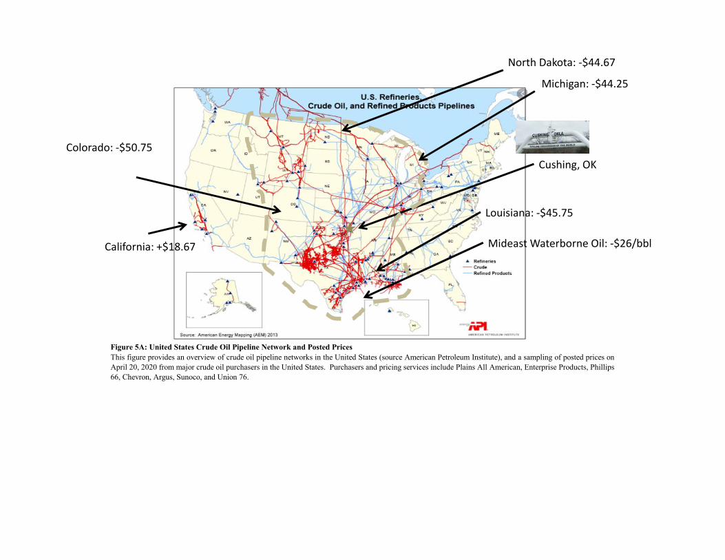
Figure 5A: United States Crude Oil Pipeline Network and Posted PricesThis figure provides an overview of crude oil pipeline networks in the United States (source American Petroleum Institute), and a sampling of posted prices onApril 20, 2020 from major crude oil purchasers in the United States. Purchasers and pricing services include Plains All American, Enterprise Products, Phillips66, Chevron, Argus, Sunoco, and Union 76.

Cushing, OK

Mideast Waterborne Oil: ‐$26/bbl

North Dakota: ‐$44.67

Colorado: ‐$50.75

Michigan: ‐$44.25

California: +$18.67

Louisiana: ‐$45.75

Figure 5B: Refinery Utilization in the United States by Region

50

55

60

65

70

75

80

85

90

95

Feb 28, 2020 Mar 06, 2020Mar 13, 2020Mar 20, 2020Mar 27, 2020 Apr 03, 2020 Apr 10, 2020 Apr 17, 2020 Apr 24, 2020 May 01, 2020May 08, 2020May 15, 2020May 22, 2020May 29, 2020

Refin

ery Pe

rcen

tage Utilization

Gulf Coast Midwest Rocky Mountain West Coast

Figure 5C: Crude Oil Storage Utilization in the United States by Region

50

55

60

65

70

75

80

85

90

95

Feb 28, 2020 Mar 06, 2020 Mar 13, 2020 Mar 20, 2020 Mar 27, 2020 Apr 03, 2020 Apr 10, 2020 Apr 17, 2020 Apr 24, 2020 May 01, 2020May 08, 2020May 15, 2020May 22, 2020May 29, 2020

Storage Ta

nk Percent Utilization

Cushing Central US Excluding Cushing West Coast

Figure 6: United States Crude Oil Posted Prices on April 20, 2020This figure plots a histogram for posted prices on 101 different crude grade/location combinations in the United States. Data was collected from posted pricesfrom the main crude oil purchasers and pricing services in the United States, which are Plains All American, Enterprise Products, Phillips 66, Chevron, Argus,Sunoco, and Union 76.

0

5

10

15

20

25

30

‐52 ‐50 ‐48 ‐46 ‐44 ‐42 ‐40 ‐38 ‐36 ‐34 ‐32 ‐30 ‐28 ‐26 ‐24 ‐22 ‐20 ‐18 ‐16 ‐14 ‐12 ‐10 ‐8 ‐6 ‐4 ‐2 0 2 4 6 8 10 12 14 16 18 20 22 24

Freq

uency

Oil Price $/BBL

All California Prices

Figure 7: Benchmark Oil Prices in 2020This figure plots several different benchmark prices for crude oil in the first half of 2020. West Texas Intermediate and Bakken grades are United Statesbenchmark prices. Edmonton is the main Canadian crude grade for crude oil of similar quality to WTI. Brent is an international crude grade of similar qualityto WTI and closely linked with crude posted prices in California.

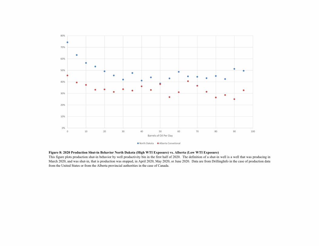
Figure 8: 2020 Production Shut-in Behavior North Dakota (High WTI Exposure) vs. Alberta (Low WTI Exposure)This figure plots production shut-in behavior by well productivity bin in the first half of 2020. The definition of a shut-in well is a well that was producing inMarch 2020, and was shut-in, that is production was stopped, in April 2020, May 2020, or June 2020. Data are from DrillingInfo in the case of production datafrom the United States or from the Alberta provincial authorities in the case of Canada.

0%

10%

20%

30%

40%

50%

60%

70%

80%

0 10 20 30 40 50 60 70 80 90 100

Barrels of Oil Per Day

North Dakota Alberta Convetional

Figure 9: 2019 Production Shut-in Behavior North Dakota (High WTI Exposure) vs. Canada (Low WTI Exposure)This figure plots production shut-in behavior by well productivity bin in the first half of 2019. The definition of a shut-in well is a well that was producing inMarch 2019, and was shut-in, that is production was stopped, in April 2019, May 2019, or June 2019. Data are from DrillingInfo in the case of production datafrom the United States or from the Alberta provincial authorities in the case of Canada.

Figure 10 Panel A: Shut-in Decisions April 2020This figure is a plot similar to Figure 9, except that it relates only to shut-in decisions in April 2020, and not May and June 2020.

Figure 10 Panel B: Shut-in Decisions May 2020This figure is a plot similar to Figure 9, except that it relates only to shut-in decisions in May 2020, and not April and June 2020.

Figure 11: Parallel TrendsThis figure plots shut-in decisions throughout 2019 comparing California to North Dakota to assess parallel trends.

Figure 12: Daily Oil Production Proxies April 2020 and May 2020This data plots natural gas that is "associated" meaning it is produced along with oil in states with large amounts of oil production, compared to dry gas states,which are states with minimal oil production and where most gas is produced from majority gas wells. The plots are normalized to 1 as of April 30, 2020. Thechange in "associated" gas is an indication of how wells that produce both

Figure 13: Daily Oil Production Proxies May 2020This figure reports "associated" gas during May of 2020. The date of the June futures contract roll, which occurs in May, is circled in red.

Table 1: Summary Statistics

North Dakota Alberta California Cushing, OK

Number of Wells 17,211 49,662 42,807 NMNumber of Firms 118 388 252 NMCrude Purchase Agreements Indexed to WTI? YES NO NO YES

Well Characteristics (2019)Average Monthly Shut-in % 13% 7% 14% NMStandard Deviation of Shut-in % 33% 25% 35% NMAverage Monthly Oil Production 2,779 335 292 NMStandard Deviation of Oil Production 5,399 913 546 NM

Crude Oil Market FundamentalsOil Price April 20, 2020 -$37.63 $10.22 $16.40 -$37.63Oil Price April 1, 2020 $8.98 $8.33 $18.84 $20.48Average Realized Oil Price April 2020 $9.64 $9.02 $20.24 $16.52Oil Price May 1, 2020 $22.28 $17.39 $20.31 $18.84Average Realized Oil Price May 2020 $29.55 $26.31 $29.21 $28.55

Refinery Utilization March 1, 2020 88% NA 85% NMRefinery Utilization April 1, 2020 74% NA 69% NMRefinery Utilization April 20, 2020 65% NA 61% NMRefinery Utilization May 1, 2020 74% NA 60% NM

Crude Oil Storage Utilization March 1, 2020 60% NA 77% 49.95%Crude Oil Storage Utilization April 1, 2020 63% NA 82% 64.93%Crude Oil Storage Utilization April 20, 2020 66% NA 87% 78.78%Crude Oil Storage Utilization May 1, 2020 68% NA 86% 86.30%

This table reports summary statistics for our empirical setting for each of the key regions of analysis. Well level data was obtained from DrillingInfo for North Dakota and California, andwas obtained from the Alberta provincial government website for Alberta. Wells in Alberta exclude oil sands wells. Crude prices were obtained from Bloomberg for North Dakota andAlberta, and from Chevron for California. Refinery utilization and crude oil storage data was obtained from the U.S. Energy Information Administration. Any data items designated "NM"are not applicable for the comparisons in the table, and any data items designated "NA" are items for which there is no data source available.

Table 2: Production Decisions and WTI Exposure in the Spring of 2020

(1) (2) (3) (4)

(β1) Postt 0.210*** 0.209*** -0.036*** -0.038***(0.026) (0.026) (0.014) (0.012)

(β2) High WTI Exposurei × Postt 0.179** 0.180** 0.425*** 0.426***(0.078) (0.078) (0.075) (0.074)

(β3) High WTI Exposurei

(β4) ln Prodi 0.026*** 0.023*** -0.013*** -0.009**(0.003) (0.002) (0.005) (0.004)

State FE Yes Yes Yes YesOperator FE No Yes No Yes

N 117391 117353 103659 103649

Absorbed by State FE

This table reports well-level regressions on decisions to stop (shut-in) production. The depdendent variable is whether well i in year t is shut-in. The estimation is a difference-in-differences regression estimation comparing the production decisions of oil wells with High WTI Exposure versus Low WTI exposure in the Spring of 2020 relative to the Spring of 2019.The dependent variable is a 1 if a well is shut-in and a 0 if the well is producing. The oil wells with high WTI exposure are located in North Dakota, whereas the oil wells with low WTIexposure are located in Alberta (specifications (1) and (2)) and California (specifications (3) and (4)). A well is designated as being shut-in if it was producing as of March in a given yearand then production ceased in April, May or June of that year. The table reports a regression form of difference-in-differences where the key coefficient of interest is the interaction term.Standard errors are clustered by firm and are reported below the coefficients in parenthesis, where *, **, *** indicate significance at the 10%, 5%, and 1% levels respectively.

Diff-in-Diff North Dakota vs. Counterfactual Area Shutin Decisions, Spring 2019 vs Spring 2020Alberta California

Table 3: Production Decisions, WTI Exposure, April 2020 vs May 2020

Panel A

April 2020 May 2020 DifferenceNorth Dakota New Shut-ins by Month 16.4% 26.5% 10.0%***

Panel B

(1) (2) (4) (5)

(β1) Postt 0.090*** 0.087*** 0.104*** 0.106***(0.009) (0.009) (0.023) (0.025)

(β2) High WTI Exposurei × Postt 0.033 0.038 0.128** 0.126**(0.033) (0.033) (0.053) (0.053)


(β4) ln Prodj 0.005*** 0.004*** 0.015*** 0.014***(0.002) (0.001) (0.002) (0.002)


N 117391 117353 117391 117353

This table reports results on shut-in behavior by month. Specifically, Panel A reports new shut-ins by month in North Dakota for April 2020 and May 2020. Panel B reports a regressionspecification similar to Table 2, except that the dependent variable of interest is month specific (instead of April/May/June shut-ins being grouped together). Panel B looks at month specificshut-ins comparing North Dakota to Alberta, while Panel C reports month specific shut-ins comparing North Dakota to California. Standard errors are reported below the coefficients inparenthesis and are clustered at the firm level, where *, **, *** indicate significance at the 10%, 5%, and 1% levels respectively.

Diff-in-Diff North Dakota vs. Alberta Shut-in Decisions, Spring 2019 vs Spring 2020April 2019 vs April 2020 May 2019 vs. May 2020


Table 3: Production Decisions, WTI Exposure, April 2020 vs May 2020

Panel C

(1) (2) (3) (4) (5) (6)

(β1) Postt -0.019*** -0.022*** -0.023*** -0.000 -0.002 -0.003(0.007) (0.007) (0.007) (0.010) (0.009) (0.009)

(β2) High WTI Exposurei × Postt 0.142*** 0.145*** 0.145*** 0.232*** 0.233*** 0.235***(0.032) (0.032) (0.033) (0.049) (0.048) (0.048)


(β4) ln Prodj -0.016*** -0.014*** -0.015*** -0.000 0.003 0.003(0.004) (0.004) (0.004) (0.002) (0.002) (0.002)

State FE Yes Yes Yes Yes Yes YesOperator FE No Yes Yes No Yes Yes

N 103659 103649 103638 103659 103649 103638

Diff-in-Diff North Dakota vs. California Shutin Decisions, Spring 2019 vs Spring 2020April 2019 vs April 2020 May 2019 vs. May 2020


Table 4: Production Decisions and WTI Exposure, Placebo Events

(1) (2) (3) (4)

(β1) Postt -0.008** -0.007** -0.015* -0.014*(0.004) (0.003) (0.008) (0.008)

(β2) High WTI Exposurei × Postt 0.006 0.006 0.013 0.012(0.008) (0.008) (0.011) (0.011)


(β4) ln Prodj 0.007*** 0.008*** -0.008** -0.007*(0.001) (0.001) (0.004) (0.004)


N 119295 119277 117019 117012

This table reports a regression specification similar to Table 2, but uses placebo time periods. Specifically, instead of focusing on the difference in shut-in behavior between the Spring of 2019and the Spring of 2020, this table reports the difference in shut-in behavior between the Spring of 2019 and Summer of 2019. Standard errors are clustered by firm and reported below thecoefficients in parenthesis, where *, **, *** indicate significance at the 10%, 5%, and 1% levels respectively.

Diff-in-Diff North Dakota vs. Counterfactual Area Shut-in Decisions, Spring 2019 vs Summer 2019Alberta California


the day that wti died: asset prices and firm production

Documents