The Deposits Channel of Monetary Policy

Itamar Drechsler, Alexi Savov, and Philipp Schnabl ∗

First draft: November 2014

This draft: March 2015

Abstract

We propose and test a new channel for the transmission of monetary policy. Weshow that when the Fed funds rate increases, banks widen the interest spreads theycharge on deposits, and deposits flow out of the banking system. We present a model inwhich imperfect competition among banks gives rise to these relationships. An increasein the nominal interest rate increases banks’ market power, inducing them to increasedeposit spreads and hence restrict deposit supply. Households respond to the increasein deposit prices by substituting from deposits into less liquid, but higher-yielding as-sets. Using branch-level data on the universe of U.S. banks, we show that followingan increase in the Fed funds rate, deposit spreads increase by more, and supply fallsmore, in areas with less deposit competition. We control for changes in banks’ lendingopportunities by comparing branches of the same bank in the same state. We controlfor changes in macroeconomic conditions by showing that deposit spreads widen im-mediately after a rate change and even if this change is fully anticipated. Our resultsimply that monetary policy has a significant impact on how the financial system isfunded, on the quantity of safe and liquid assets it produces, and on its provision ofloans to the real economy.

Keywords: Monetary policy, deposits, market power, safe assets, liquidity, privatemoney, real effects

∗New York University Stern School of Business, idrechsl@stern.nyu.edu, asavov@stern.nyu.edu, andpschnabl@stern.nyu.edu. Drechsler and Savov are also with NBER, Schnabl is also with NBER and CEPR.We thank Siddharth Vij for excellent research assistance. We thank Arvind Krishnamurthy, David Scharf-stein, Jeremy Stein and seminar participants at Harvard University, NYU-Columbia Junior Meeting, StanfordUniversity, University of Montreal, and Temple University for helpful comments.

I. Introduction

We propose and test a new channel for how monetary policy affects the financial system

and the real economy. We show that when the Fed funds rate increases, banks widen the

interest spreads they charge on deposits and deposits flow out of the banking system. These

relationships are strong and the aggregate effects large, suggesting that monetary policy has

a significant impact on how the financial system is funded, and on the quantity of safe and

liquid assets it produces. We argue that these relationships are due to imperfect competition

among banks, i.e., market power, in the provision of liquid deposits. An increase in the

nominal interest rate effectively increases banks’ market power, to which banks respond

by increasing the spread they charge on deposits. As deposits become more expensive,

households reduce their deposit holdings and replace them with imperfect substitutes, higher

yielding but lower-liquidity assets. Using branch-level data on geographical variation in

competitiveness of local deposit markets, we document this channel and argue that the

relationship to monetary policy is indeed causal.

The implications of this channel are significant because deposits are special to both banks

and households. Deposits have historically been–and continue to be–far and away the most

important single source of funding for the banking system. In 2014, they amount to roughly

$10.2 trillion, or 77% of bank liabilities. As we report below, banks earn large spreads

on deposits. Deposits are also much more persistent (“sticky”) than the financial system’s

alternative funding sources, mainly short-term wholesale markets, and may therefore confer

banks with an advantage in investing in illiquid and risky assets (Hanson, Shleifer, Stein, and

Vishny 2014). For households, deposits represent the main source of safe and liquid assets

and therefore changes in the price and supply of deposits will affect the price of other major

types of safe and liquid assets, including Treasuries. The deposits channel we document can

therefore explain how monetary policy can affect the premium on all safe and liquid assets.1

Figure 1 plots the time series of the Fed Funds rate and the average rate paid by three

deposit products: interest checking, money market saving account, and 12-month certificate

of deposits (CD). These three products proxy respectively for the three major classes of

1Krishnamurthy and Vissing-Jorgensen (2012) show that Treasury prices embed a large liquidity premiumand document that this premium varies inversely with Treasury supply.

1

bank deposits: checking deposits, savings deposits, and time deposits, which accounted for

$1.6 trillion, $6.5 trillion, and $2.1 trillion in 2014, respectively.

Figures 1 shows two striking regularities. First, the spreads between the Fed funds rate

and the deposit rates are often very large, especially for checking and savings deposits. In

particular, the spread on savings deposits, which constitutes almost half of all deposits, is

greater than 2% on average over this period, and at times exceeds 3%. Checking deposits

incur a substantially larger spread still, whereas the spread on time deposits is relatively

small. Second, deposit spreads covary strongly positively with the Fed funds rate. When

the Fed funds rate increases, banks increase deposit rates, but less than one-for-one, so that

spreads widen.2 In contrast, when the Fed funds rate decreases, deposit spreads shrink. For

instance, as the Fed Funds rate dropped from 6.5% in 2000 to 1% in 2004, the spread on

savings deposits shrank from 3% to 0.25%. As with average spreads, the pattern in checking

deposits is even more pronounced, whereas it is less dramatic for time deposits.

Figure 2 shows the resulting adjustment for the equilibrium quantities of deposits. It

plots year-over-year percentage changes in the Fed funds rate against the growth in the

aggregate quantity of savings deposits (Panel A), checking deposits (Panel B), time deposits

(Panel C), and total deposits (Panel D). The relationships are clear and striking. Panel A

shows that changes in the Fed funds rate are strongly negatively related to the growth rate in

savings deposits. Hence, as the deposit spread increases, depositors reduce their holdings of

savings deposits. Panel B shows a similar relationship for checking deposits. The effects are

economically significant in both cases; fluctuations in year-over-year deposits growth range

from -14% and +26%, a large amount given the enormous size of total deposits.

Panel C shows that the opposite relationship holds for time deposits: changes in the Fed

funds rate are positively related to the growth in time deposits. There appears, therefore, to

be an important difference between how depositors treat time deposits relative to checking

and savings deposits. Recognizing this difference is important for our theory and empirical

analysis. For this reason, which reflects the differences in their demandability and other

features as well as their usage, we refer to savings and checking deposits as “liquid deposits”

and contrast them with time deposits. Hence, when the Fed funds rate rises, the spreads on

2This gives the impression that deposit rates are “sticky” (Discoll and Judson 2013).

2

liquid deposits widen relative to time deposits, and depositors substitute away from liquid

deposits and toward less liquid time deposits.

Panel D shows the relationship for total deposits. Changes in the Fed funds rate are

strongly negatively related to the growth in total deposits, reflecting the fact that checking

and savings deposits account for the majority of total deposits. This shows that the aggregate

outflows from liquid deposits exceed the aggregate inflows to time deposits. On net, it follows

that when the Fed funds rate increases, total deposits shrink.

We develop a model that explains these relationships and guides our empirical analysis.

In the model, banks are monopolistic competitors that have market power over the creation

of deposits. Two assets represent imperfect substitutes to deposits; cash (currency or non-

interest-bearing accounts), which is completely liquid but pays no interest, and bonds, which

provide no (or less) liquidity services but pay a higher, competitive interest rate. As the

interest rate increases, cash becomes more expensive to hold and represents a less attractive

alternative to deposits as a source of liquidity. Hence, an increase in the nominal interest

rate effectively increases banks’ market power in liquidity provision. This is especially true in

concentrated markets where competition among banks is low. Banks in such markets respond

by charging higher deposit spreads, giving rise to the relationship in Figure 1. Households

respond to the higher prices by substituting away from liquid deposits to less-liquid deposits

and bonds, giving rise to the relationships shown in Figure 2.

Next, we examine empirically whether monetary policy indeed causes changes in deposit

supply, driving the relationships in Figures 1 and 2. The main identification concern is that

monetary policy reacts to macroeconomic conditions, which may directly affect both banks’

supply of deposits and households’ demand for deposits. For example, monetary policy

tends to tighten when inflation rises and higher inflation may also reduce banks’ lending

opportunities, which in turn lowers banks’ funding needs and thus reduces their deposit

supply. This could give rise to the observed aggregate relationships between the Fed funds

rate and deposits, even in the absence of a deposits channel of monetary policy.

To address this identification challenge, we exploit geographical variation in the degree

of competition across U.S. counties. The intuition is that an increase in the Fed funds

rate has a larger effect on banks’ market power in areas with low competition and thus

3

leads to higher spreads and larger outflows in those areas. We implement this identification

strategy by computing the Herfindahl index based on county-level deposit market shares as

a measure of local deposit competition. We then analyze whether an increase in the Fed

funds rate raises deposit spreads and outflows more in concentrated markets relative to less

concentrated markets.

Importantly, we control for banks’ lending opportunities by using information from dif-

ferent branches of the same bank. To illustrate our approach, consider a bank with branches

in two counties. The bank’s lending opportunities may change after a Fed funds rate change

because of underlying changes in the economy. We control for such changes by including

a full set of bank-time fixed effects in our estimation. This approach adjusts for any un-

observed variation in a bank’s willingness to supply deposits and identifies the effect of the

Fed funds rate on deposits using only within-bank variation across counties. The identifying

assumption is that a deposit raised at one branch can be used as funding at another branch

of the same bank. Under this assumption, changes in a bank’s lending opportunities affect

all branches equally, allowing us to control for the effect of macroeconomic conditions on

deposits.

We implement this strategy using quarterly branch-level data on deposit rates and hold-

ings for the most widely offered savings and time deposit products. Our estimates suggest

that after a 100 basis point increase in the Fed funds rate, branches in concentrated markets

increase savings deposit spreads by 12 basis points and time deposits spreads by 5 basis

point relative to branches located in less concentrated markets. We also find that branches

in concentrated markets experience a deposit outflow of 78 basis points relative to branches

in less concentrated markets. All results are statistically significant.

These results indicate that monetary policy on net affects the supply of deposits: an

increase in the Fed funds rate leads to higher deposit spreads and less total deposits. We

point out that this result is inconsistent with an effect of monetary policy on household

demand for deposits. Otherwise one would expected that deposit spreads (price) and total

deposits (quantity) move in the same direction. Put differently, the results indicate that

monetary policy works through changes in the banks’ willingness to supply deposits rather

than changes in households’ demand for deposits.

4

To better understand the effect of monetary policy, we examine its timing using weekly

data on deposit rates. We find that changes in monetary policy affect deposit rates exactly

at the time of the change in the Fed Funds rate. The difference across more and less

concentrated deposit markets appears quickly–within a week or two–after Fed funds changes.

This result provides further evidence in support of a direct effect of the Fed funds rate on

deposits because for other economic variables to explain our results their timing would have

to coincide very closely with changes in the Fed funds rate.

Next, we examine the mechanism of how monetary policy affects the supply of deposits.

Our theory suggests that monetary policy works trough its effect on banks’ market power.

As an alternative theory, changes in deposit supply may be driven by information that the

Federal Reserve releases at the time of rate change announcements. This perspective implies

that the Federal Reserve does not control interest rates, but signals information through rate

changes.3 The challenge of distinguishing between the two explanations is a common issue

in empirical studies of monetary policy because any rate announcement may reveal private

information.

We are able to provide evidence on the mechanism by testing whether deposit spreads

respond to expected changes in the Fed funds rate, as measured using Fed funds futures prices

prior to the rate announcements. Whereas in most financial settings anticipated changes have

no effect on prices because prices react to news rather than realizations, in our setting they

react to both. The reason is that liquid deposits and the Fed funds rate have zero maturity,

and hence the impact of changes is not incorporated until their actual realization, even if

these changes are anticipated. This unique feature of our setting allows us to test whether

monetary policy works through changes in the interest rate rather than the release of private

information. Indeed, we find that our main results are similar if we only use variation in

expected changes in monetary policy.

These results also provide additional identification for our main results. If other economic

variables affect the supply of deposits, their effect would have to appear exactly at the time

of the anticipated rate change. It is hard to think of an alternative transmission channel

that allows for economic variables to prompt changes in expectations about monetary policy

3Fama (2013) argues in favor of this viewpoint.

5

but only affects deposit supply once the changes are implemented.

Finally, as an alternative check on our results, we provide an additional identification

test by exploiting a unique feature of our data. Some smaller branches do not set their own

deposit rates but rather follow larger branches, some of which are located in other counties.

Under the assumption that large banks set rates based on local deposit markets, we can use

the deposit competitiveness of rate-setting branches as an instrument for deposit rates at

non-rate setting branches and examine its effect on deposit flows. Using branch-level data

on the link between rate-setting and non-rate-setting branches, we find that branches that

follow rates from less competitive counties experiences larger deposit outflows than those

that follow rates from more competitive counties. This finding provides direct evidence on

the deposits channel of monetary policy.

We then verify whether our branch-level results aggregate up to the bank-level. This

is useful for several reasons. First, it allows us to quantify whether changes in deposits

are sufficiently large to affect banks’ total funding. Second, we can extend our analysis

to the asset side of bank of bank balance sheets and examine its effect on lending. This

is important to understand the real effects of the deposits channel. Third, we can verify

whether our results are robust to control variables that proxy for alternative channels of

monetary policy.

We construct a bank-level measure of deposit competition by aggregating across branches

and weighting by deposits. On the liabilities side, we find that the results on deposits are

qualitatively and quantitatively similar to the ones at the branch level. A 100 basis point

increase in the Fed Funds rate leads to 1.5% larger outflow in deposits in uncompetitive

markets relative to competitive markets. On the asset side, we find that after a 100 basis

points increase in the Fed funds rate, banks operating in uncompetitive markets reduce

assets by 1.0%, and real estate lending by 0.7%, relative to banks operating in competitive

markets. The results are robust to controlling for bank fixed effects and time-varying bank

characteristics such as leverage and security holdings. These results indicate that monetary

policy affects banks’ lending through its effect on deposits.

We conduct several robustness test of our main results. First, we find that the results

are robust to using alternative measures of market competition such as deposit competition

6

based on the number of bank branches. Second, we show that the main results are robust

to controlling for state-specific, non-parametric time trends, which rules out the effect of

confounding state-level factors (e.g., regulatory or political changes). Third, we find that

the results are similar and larger, if we estimate the effect using variation across banks.

This paper connects to large theoretical and empirical literatures on the transmission

of monetary policy to the real economy, the bank lending channel, and private money cre-

ation. Bernanke (1983) documents the importance of bank lending for the propagation of

macroeconomic shocks. Bernanke and Gertler (1995) and Kashyap and Stein (1994) formal-

ize the bank lending channel. Kashyap, Stein, and Wilcox (1992) provide evidence based

on the behavior of bank lending. Bernanke and Gertler (1989) and Bernanke, Gertler, and

Gilchrist (1999) present a broader balance sheet channel that works through limited capital

in the financial sector. More recently, He and Krishnamurthy (2013) and Brunnermeier and

Sannikov (2014) present fully dynamic macroeconomic models with intermediation frictions.

On the empirical side, Bernanke and Blinder (1992) show that in aggregate time series

data an increase in the Fed funds rate is associated with an increase in unemployment and a

decline in deposits. Kashyap and Stein (2000) find that small banks with less liquid balance

sheets reduce lending more after a rate increase. Jimenez, Ongena, Peydro, and Saurina

(2014) and Dell’Ariccia, Laeven, and Suarez (2013) show that monetary policy impacts bank

lending decisions by exploiting within bank variation in borrower characteristics. Scharfstein

and Sunderam (2014) show that market power in mortgage lending affects the sensitivity of

such lending to monetary policy.

Diamond and Dybvig (1983) interpret banks as liquidity providers to households through

demand deposits. Kashyap, Rajan, and Stein (2002) study the complementarity between

taking deposits and making loans. Consistent with the liquidity provision role of the banking

sector, Krishnamurthy and Vissing-Jorgensen (2012, 2013) show that Treasury bill rates

incorporate liquidity premia and that bank balance sheets compensate for reductions in the

supply of Treasuries. Sunderam (2012) shows that the shadow banking system also responds

to liquidity premia. Nagel (2014) links the rates on money market instruments to the cost

of liquidity as measured by the Fed funds rate.

Discoll and Judson (2013) show that deposit rates are “sticky” and their adjustment to

7

market rates is asymmetric. Acharya and Mora (2014) document a large reallocation of

deposits across banks during the financial crisis. Ben-David, Palvia, and Spatt (2014) and

Gilje, Loutskina, and Strahan (2013) show that banks channel deposits across branches to

areas with high loan demand. Stein (1998) argues that deposit funding is difficult to replace

with wholesale funding and examines the implications for monetary policy transmission.

Stein (2012) presents a model that shows how monetary policy can regulate private liquidity

creation. Drechsler, Savov, and Schnabl (2014) connect monetary policy and bank risk taking

in a dynamic asset pricing framework.

A branch of the empirical literature on monetary policy and asset prices uses the event

study methodology. Bernanke and Kuttner (2005), Hanson and Stein (2012), and Gertler

and Karadi (2014) show that nominal rates have large effects on risky assets such as stocks,

long-term bonds, and credit spreads.

The broad contribution of our paper is two fold: to show that deposit taking transmits

monetary policy to the real economy via the banking system, and to demonstrate how this

channel works through imperfect competition in private liquidity provision.

The rest of this paper is organized as follows: Section II presents our model, Section III

summarizes our data, Section IV presents our results, and Section V concludes.

II. Model

We present a simple model that captures the relationships between bank competition, de-

posits, and the nominal interest rate. For simplicity, the economy lasts for one period and

there is no risk. We think of this economy as corresponding to a well-defined regional market,

or county, in the context of our empirical analysis.

The county’s representative household maximizes utility, defined over final wealth, W ,

and liquidity services, v, according to the following CES aggregator:

U (W0) = maxM,D

u (W, v) (1)

u (W, v) =[W

ρ−1ρ + αv

ρ−1ρ

] ρρ−1

, (2)

8

where α is a share parameter, and ρ is the elasticity of substitution between wealth and

liquidity. Such a preference for liquidity arises in many models. For example, it arises in

many monetary models as a consequence of a cash-in-advance constraint (see Galı 2009). In

other models it arises as a preference for extreme safety (e.g., Stein 2012) . In both cases, it

is natural to think of wealth and liquidity as complementary, so that ρ < 1.

Liquidity services are in turn derived from holding cash M and deposits D according to

a CES aggregator:

v (M,D) =[M

ε−1ε + δD

ε−1ε

] εε−1

, (3)

where ε is the elasticity of substitution and 0 ≤ δ < 1 measures the relative contribution

of deposits to liquidity. We interpret cash as consisting of currency and zero-interest check-

ing accounts. In contrast, deposits pay a rate of interest, determined in equilibrium. We

interpret deposits as consisting of savings deposits and small time deposits offered to house-

holds.4 Because they both provide liquidity, it is most natural to view cash and deposits as

substitutes, so that ε > 1.

The county’s deposits are themselves a composite good produced by the N banks in the

county,

D =

(1

N

N∑i=1

Dη−1η

i

) ηη−1

, (4)

where η is the elasticity of substitution between banks. Each bank has mass 1/N and pro-

duces deposits at the intensity Di, resulting in an amount Di/N . If all the intensities are

identical, then Di = D. When N → ∞, the aggregator becomes the usual Dixit-Stiglitz

aggregator. Because deposits at different banks are substitutes, η > 1. The imperfect

substitutability (η < ∞) between deposits creates monopolistic competition, giving banks

market power and allowing them to sustain nonzero profit margins. Although we model a

representative county household, the aggregator can be interpreted as representing a county

populated by individual households. Each household has a preference for keeping deposits

4For simplicity, we only have a single type of deposit. One could extent the model to allow for depositsof varying degree of liquidity.

9

at the most convenient bank, but can substitute (imperfectly) to other banks. Hence, house-

holds aggregate into a representative household that substitutes deposits imperfectly across

banks and prefers to distribute deposits evenly.

Each bank charges a deposit spread si and so pays a deposit rate f − si, where f is the

Fed funds rate set by the central bank and is equal to the rate of return on bonds. Let W0

be the initial wealth of the household. Terminal wealth is then given by

W =

(W0 −M −

1

N

N∑i=1

Di

)(1 + f) +M +

1

N

N∑i=1

Di (1 + f − si) (5)

= W0 (1 + f)−Mf − 1

N

N∑i=1

Disi. (6)

If we define the weighted average spread on deposits as s = 1N

∑Ni=1

DiDsi, then this equation

can be written as

W = W0 (1 + f)−Mf −Ds. (7)

In words, households earn the bond interest rate on their initial wealth while foregoing all

interest on their cash holdings and the deposit spread on their deposits.

The household’s optimality choices can be summarized by three conditions. The first

condition is the interbank substitution margin,

Di

D=

(sis

)−η. (8)

In words, as a bank increases its deposit spread (relative to other banks), the household

reduces deposits at the bank at the rate η, the elasticity of substitution across banks. The

second condition is the cash-deposits substitution margin,

D

M= δε

(s

f

)−ε. (9)

It says that when deposits spreads are high, households substitute away from deposits and

into cash at the rate ε, the cash-deposits elasticity. Finally, the cash-bonds substitution

10

margin is

M

W= αρf−ρ

[1 + δε

(f

s

)ε−1] ρ−εε−1

. (10)

When the fed funds rate is high, and therefore cash is expensive, households hold less cash

and more bonds. However, just how much depends also on the relative cost of deposits (f/s).

Banks raise deposits and invest in bonds, which yield a higher rate. More generally we

can think of banks investing in a portfolio of risky loans with the same risk-adjusted return

as safe bonds. Banks set their deposit spreads to maximize profits:

maxsi

siDi. (11)

The profit-maximizing condition is

∂Di/Di

∂si/si= −1. (12)

In words, at the optimal deposit spread the elasticity of deposits with respect to the spread

is precisely -1, and hence further adjustment of the spread cannot increase the bank’s profits.

We can use the interbank margin (8) to calculate the elasticity in (12):

∂Di/Di

∂si/si=

(∂D/D

∂s/s

)(1

N

Di

D

sis

)− η

(1− 1

N

Di

D

sis

). (13)

In a symmetric equilibrium (Di = D and si = s) this becomes

∂Di/Di

∂si/si=

1

N

(∂D/D

∂s/s

)− η

(1− 1

N

). (14)

As bank i increases its spread si, it faces outflows from two sources. The first is an aggregate

effect: the increase raises the average deposit spread, making deposits more expensive. This

leads to outflows from deposits as an asset class. This effect diminishes as banks become more

numerous because each individual bank is less important. The second source of outflows is

due to competition among banks and is bank-specific: raising si increases the deposit spread

11

of bank i relative to the average deposit spread. When bank i raises its spread by one

percent, the average spread goes up by 1/N percent, and hence the relative spread of bank

i increases by 1 − 1/N . This induces an outflow of deposits at a rate η, the elasticity of

substitution across banks.

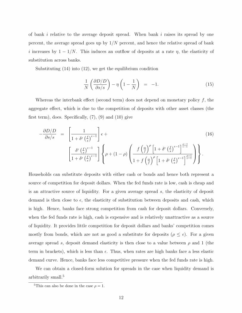
Substituting (14) into (12), we get the equilibrium condition

1

N

(∂D/D

∂s/s

)− η

(1− 1

N

)= −1. (15)

Whereas the interbank effect (second term) does not depend on monetary policy f , the

aggregate effect, which is due to the competition of deposits with other asset classes (the

first term), does. Specifically, (7), (9) and (10) give

−∂D/D∂s/s

=

[1

1 + δε(fs

)ε−1]ε+ (16)

[δε(fs

)ε−11 + δε

(fs

)ε−1]ρ+ (1− ρ)

f(αf

)ρ [1 + δε

(fs

)ε−1] ρ−1ε−1

1 + f(αf

)ρ [1 + δε

(fs

)ε−1] ρ−1ε−1

.

Households can substitute deposits with either cash or bonds and hence both represent a

source of competition for deposit dollars. When the fed funds rate is low, cash is cheap and

is an attractive source of liquidity. For a given average spread s, the elasticity of deposit

demand is then close to ε, the elasticity of substitution between deposits and cash, which

is high. Hence, banks face strong competition from cash for deposit dollars. Conversely,

when the fed funds rate is high, cash is expensive and is relatively unattractive as a source

of liquidity. It provides little competition for deposit dollars and banks’ competition comes

mostly from bonds, which are not as good a substitute for deposits (ρ ≤ ε). For a given

average spread s, deposit demand elasticity is then close to a value between ρ and 1 (the

term in brackets), which is less than ε. Thus, when rates are high banks face a less elastic

demand curve. Hence, banks face less competitive pressure when the fed funds rate is high.

We can obtain a closed-form solution for spreads in the case when liquidity demand is

arbitrarily small.5

5This can also be done in the case ρ = 1.

12

Proposition 1. Let ρ < 1 < ε and η > 1. Denote by M the quantity 1 − (η − 1)(N − 1),

which captures the effective market power of the banking sector. Consider the limiting case

α→ 0. If M < ρ then the deposit spread is zero. Otherwise the deposit spread is

s = δεε−1

(M− ρε−M

) 1ε−1

f, (17)

The deposit spread:

(i) increases in banks’ market power M, which is itself decreasing in the number of banks

N and elasticity of substitution across banks η

(ii) increases with the fed funds rate f

(iii) increases more with the fed funds rate when the banking sector’s market power is higher

Proof of Proposition 1. It follows from (15) that when banks’ equilibrium choice is internal,

the aggregate deposit elasticity satisfies −∂D/D∂s/s

= 1 − (η − 1)(N − 1) = M. Equation

(17) follows by substituting (16) into this expression and letting α → 0. The relationship

between s andM is ∂s∂M = s(ε−1)−1 (ε−M)−2. Thus s increases inM provided that ε > 1.

Moreover, M decreases in N and η provided N, η > 1. Using ∂2s∂M∂f

= 1s∂s∂f

∂s∂M and ∂s

∂f> 0

gives (iii).

Competition among banks leads to the banking sector as a whole having an effective

market power given by the endogenous quantityM. This market power decreases when there

is more competition, either because there are more banks (N is higher), or because bank

deposits are more easily substituted across banks (η is larger). One way to interpret the result

of the proposition is to replace the banking sector with an hypothetical representative bank

with this level of market power. The equilibrium deposit spread is the one that maximizes

this representative bank’s profits, and is given precisely by the spread at which the elasticity

of aggregate deposit demand, -∂D/D∂s/s

, equals the representative bank’s market power M.

When there is only one bank, or bank deposits are relatively hard to substitute (η → 1),

M = 1 (its largest possible value), the banking sector acts like a pure monopolist, and the

deposit spread is large. In contrast, when N is large or bank deposits are good substitutes

(η is large), M is small and the equilibrium deposit spread is small.

13

The proposition further shows that the equilibrium spread rises with the feds funds rate.

When the fed funds rate is high, cash is an expensive source of liquidity and hence an

expensive substitute for bank deposits. The representative bank’s competition comes mostly

from bonds, a relatively poor substitute for deposits (ρ < ε). Hence, the representative bank

faces a relatively inelastic demand curve and so charges more for deposits. In contrast, when

the fed funds rate is low the representative bank faces more competition from cash, which

has a high elasticity (ε > 1) with deposits. It therefore faces a relatively elastic demand

curve and hence charges less for deposits. In this way monetary policy affects the level of

external competition faced by the banking sector.

Finally, proposition 1 shows that the effect of the fed funds rate on the deposit spread

is larger where there is less competition. Where competition is intense, spreads are low

regardless of the fed funds rate and the opportunity cost of holding cash. In contrast, where

competition is weak, cash is a more important alternative to bank deposits, and hence the

effect of the fed funds rate on deposit spreads is stronger. This effect is captured by the

cross-partial in part (iii) of Proposition 1 and corresponds empirically to the the coefficient

on the interaction of market power and changes in the fed funds rate that we estimate in

the deposit rate regressions below.

III. Data and Summary Statistics

We build a novel data set at the bank-branch level that includes information on deposits

rates (by product), deposit holdings, branch ownership, bank characteristics, and county

characteristics.

The data on deposit holdings is from the Federal Deposit Insurance Fund (FDIC). The

FDIC provides annual branch-level data on total deposits outstanding from June 1994 to

June 2014. The data set has information on branch characteristics such as the branch owner-

ship, the branch address, and the branch’s geographic coordinates (latitude and longitude).

The data covers the universe of bank branches in the U.S. and contains a unique branch

identifier, bank identifier, and county identifier. We use these identifiers to match the data

with other data sets.

14

The data on deposit rates is from the private data provider Ratewatch. Ratewatch

collects weekly branch-level data on deposit rates by branch and product. The data is a

representative sample of U.S. branches with a coverage of 54% in 2008. We merge the

Ratewatch data with the FDIC data using the unique FDIC branch identifier. We are able

to match 85.4% of the data collected by Ratewatch.

The Ratewatch data reports a deposit rate if a specific product is offered by a branch.

We focus our analysis on the two deposit products that are most widely offered across all

branches, 10K money market account and 12-month 10K certificates of deposit. These two

products are representative of the two main types of deposits (savings and time). We confirm

in robustness tests that our results also hold for other deposit products.

The Ratewatch data reports whether a branch actively sets deposit rates (“rate setter”)

or whether a branch uses rates that are set by another branch (“non-rate setter”). The data

provides a link between non-ratesetting and ratesetting branches. Each non-rate setter is

linked to a single rate setter, while rate setters can be linked to more than one non-rate

setter. Non-rate setters are mostly smaller branches that are geographically close to the

ratesetting branch. Most of our analysis focuses on the active setting of deposit rates and

we therefore focus on the sample of rate setters. We use the sample of non-rate setters for a

separate empirical test.

We collect data on county characteristics from several sources. The data on the annual

number of establishments, employment, and annual payroll are from the County Business

Patterns survey, the data on quarterly wages are from the Bureau of Labor Statistics, and

the data on annual population and county size are from the Census Bureau. We also collect

data on annual gross county tax revenues from the Internal Revenue Services and data on

annual median household income, the unemployment rate, and the poverty rate from the

Census Bureau. We merge the county-level data with the deposit data using the FDIC

county identifier. The data covers all counties with at least one bank branch.

We collect the data on bank characteristics from the U.S. Call Reports, obtained from

the Federal Reserve Bank of Chicago. U.S. Call Reports include quarterly bank-level data

on income statements and balance sheets data for all U.S commercial banks. To ensure

robustness against outliers, we drop observations if total assets, total deposits, or total

15

liabilities are less than $1 million or if they are missing. We match the bank-level data to

the branch-level data using the FDIC bank identifier.

Our analysis focuses on the effect of monetary policy on deposits rates and holdings. We

measure the stance of monetary policy using the Fed funds rate. We collect the quarterly

Fed funds rate (as of the end of the quarter) from the St. Louis Federal Reserve Economic

Database. For some of our analysis, we distinguish between expected and unexpected changes

in the Fed funds rate over a quarter. Following Kuttner (2001), we compute the expected

change in the Fed funds rate as the difference between the Fed funds rate and the Fed funds

future rate, both at the beginning of the quarter. The unexpected change in the monetary

policy is the actual change during a quarter minus the expected change.

Our main measure of bank competition is the deposit Herfindahl index at the county level.

We compute the deposit Herfindahl for a given county in a given year in the standard way,

i.e. by summing the squared deposit shares of all banks with branches within that county

and in that year. A Herfindahl of one indicates an extreme of complete concentration of

county deposits within a single bank, whereas lower values indicate greater competitiveness.

Figure 3 plots the variation in bank competition across counties. For each county, we

plot the average deposit Herfindahl from June 1994 to June 2008. As shown in the figure,

there is significant variation across counties ranging from highly competitive counties with

a minimum Herfindahl of 0.06 to uncompetitive counties with a maximum Herfindahl of 1.

The figure does not reveal any obvious regional clustering of bank competition. As we show

in the robustness section, our results are robust to computing the Herfindahl index based on

a number of bank branches operating in a county.

Panel A of Table 1 provides summary statistics at the county level. The data is at the

annual level from 1996 to 2008 covering all U.S. counties with at least one bank branch, which

yields a total of 46,674 observations. We focus on the period before 2008 because we are

interested in the conduct of monetary policy during regular (non-crisis) times. The average

Herfindahl index during this period is 0.354 with a standard deviation of 0.290. We provide

a breakdown of county characteristics split at the median Herfindahl index within each year.

Low-Herfindahl counties (high competition) are larger than high-Herfindahl counties (low

competition) with a median population of 49,889 versus 13,496. They also have a higher

16

median household income, $38,815 versus $33,212, and a lower poverty rate, 13.1% versus

16.2%.

Panel B of Table 1 provides summary statistics at the branch level. The data is annual

from 1996 to 2008 for all U.S. commercial banks with at least two ratesetting branches,

which yields a total of 97,751 observations. The average bank has total deposits of $122

million with an average deposit growth of 6.2%. The average deposit Herfindahl index is

0.239 with a standard deviation of 0.203. The median spread (Fed funds rate minus deposit

rate) is 1.91% for interest checking accounts, 1.66% for money market accounts, and 0.01%

for 12-month CDs. We also provide a breakdown by the median Herfindahl of 0.203 and find

that spreads are similar across high- and low-Herfindahl counties.6

Panel C of Table 1 provides summary statistics at the bank level. The data is annual

from 1996 to 2008 for the sample of all U.S. commercial banks, which yields a total of 122,821

observations. We compute a bank’s deposit Herfindahl index as the weighted average of its

branch-level Herfindahl indices using deposits as weights. The average bank has $765 million

in assets and grows at a median rate of 6.43%. The main funding source is deposits, which

account for 83.0% of the balance sheet. Demand deposits, which include checking deposits,

account for 12.8%, savings deposits account for 19.9%, and time deposits account for 39.1%.

The other funding sources are equity with an 11.1% share and non-deposit debt with a 5.9%

share.

IV. The Effect of Monetary Policy on Deposits

A. Across-branch empirical strategy

Our empirical strategy is designed to estimate the effect of monetary policy on deposits.

As shown in Figure 1, the spread between deposit rates and the Fed funds rate widens as

the Fed funds rate increases. At the same time, as shown in Figure 2, there is an outflow

6This finding is somewhat surprising given that the earlier literature on deposits found that deposit ratesare lower in less competitive areas. We find that this result holds after controlling for county-level income.This result reflects the fact that higher income counties are both more competitive and have higher spreads.This may be caused by the higher cost of operating branches in high-income areas (e.g. because of higherwages and higher rentals costs).

17

from checking and savings deposits (Panels A and B) and an inflow to time deposits (Panel

C). The net effect is an aggregate outflows of deposits from the banking system (Panel

D). Hence, when the Fed funds rate increase, total deposits shrink and the composition of

deposits becomes less liquid. This evidence is suggestive of a direct link between monetary

policy and deposit flows.

However, it is possible that omitted variables such as time-varying economic conditions

drive both monetary policy and deposit flows. For example, the Federal Reserve tends to

tighten monetary policy when inflation rises. If higher inflation also reduces banks’ lending

opportunities, then banks may supply fewer deposits when the Fed funds rate increases.

Hence, omitted variables can generate the observed aggregate relationships even in the ab-

sence of a direct effect of monetary policy on deposits.

We address this concern by exploiting differences in market power across banks. An

important insight of the model is that an increase in the Fed funds rate leads to higher

deposit spreads in areas where competition is low (see Proposition 1). Hence, we can test

the deposit channel by comparing banks in concentrated (uncompetitive) areas with banks

in less concentrated (competitive) areas. This approach controls for the average effect of

macroeconomic conditions on bank lending opportunities.

We start doing so by analyzing the sensitivity of deposit rates and flows to changes in

monetary policy. Specifically, for each county we estimate the following regression:

∆yijct = α + β∆FFt + εijct , (18)

where yijct is either the change in the deposit spread (price) or the log change in total deposits

(quantity) of branch i of bank j in county c from time t to t + 1 and ∆FFt is the change

in the Fed funds rate from time t to t+ 1. We refer to the coefficient β as the deposit beta

because it captures the average change in deposit rate and flow associated with a change in

the Fed funds rate (“deposit beta”). We then sort counties by Herfindahl index and average

deposit beta for each five-percentile increment. This yields a total of 20 point estimates,

each representing the average deposit beta for about 161 counties.

We conduct this estimation for deposit rates on money market accounts and 12-month

18

CDs because they are most widely offered deposit products across branches. We conduct

the estimation for total deposits using branch-level deposit growth. We include all branches

that report deposit rates in the Ratewatch data and deposit growth in the FDIC data,

respectively.

Panel A of Figure 4 shows the results for 10K money market accounts (savings deposits).

The figure shows that the deposit beta is larger for less competitive markets. The average

deposit beta is around 0.64 in low-Herfindahl counties (below 10th percentile) relative to

about 0.71 in high-Herfindahl counties (above 90th percentile). This means that a 100 basis

points increase in the Fed funds rate leads to a 7 basis point increase in uncompetitive

markets relative to competitive markets. The result is robust in that other markets line

up in between with a roughly linear increase in deposit beta in the Herfindahl index. The

economic magnitude is significant in that it accounts for 11% of the average increase in

deposit spreads after an increase in the Fed funds rate.

Panel B shows the result for time 12-month certificate of deposits (time deposits). We

find again that the deposit beta is larger for less competitive markets. The average deposit

beta is around 0.24 in low-Herfindahl counties (below 10th percentile) relative to about 0.28

in high-Herfindahl counties (above 90th percentile). This effect accounts for 15% of the

average difference increase in deposit spread after an increase in the Fed funds rate.

Panel C shows the result for deposit growth. In contrast to the result on prices, we find

that the deposit beta is larger in competitive markets. The average deposit beta is close

to zero in low-Herfindahl counties (below 10th percentile) relative to about -0.6 in high-

Herfindahl counties (above 90th percentile). This effect accounts for 22% of the average

difference deposit outflow after an increase in the Fed funds rate.

Importantly, these results show that an increase in the Fed funds rate leads to an in-

crease in deposit spreads (price) and a decline in outstanding deposits (quantity). This

indicates that monetary policy works through shifting the supply curve rather than shifting

the demand curve. This rules out alternative explanations that rely on shifting the demand

curve for deposits. It also provides direct support for the main prediction of our theoretical

analysis.

Yet, using variation in deposit competition across markets may not completely control

19

for macroeconomic conditions. The reason is that changes in macroeconomic conditions may

lead to different changes in banks’ lending opportunities. If the change in banks’ lending

opportunities correlates with deposit competition, then this may bias our estimation. For

example, if banks in more concentrated markets experience a large decline in lending oppor-

tunities after a Fed funds increase, then this may lower the deposit supply in concentrated

markets because banks need fewer deposits to finance loan growth. As a result, this may

lead to a supply shift in deposits for reasons other than market power.

We address this concern by exploiting geographical variation in deposit competition across

branches for the same bank. This strategy is best illustrated by an example. Consider a

bank that is operating two branches, one of which is located in a concentrated area and

one of which in a less concentrated area. We control for the bank’s lending opportunities

by comparing the deposit supply by the branch in the concentrated area with the deposit

supply by the branch in the less concentrated area. This approach controls for the average

change in the bank’s deposit supply.

The identifying assumption is that banks equalize the marginal return to lending across

branches by lending to projects with the highest expected value. This assumption is satisfied

if banks use internal capital markets to allocate resources efficiently. Even if there are

frictions in banks’ internal capital market, this strategy identifies the effect of competition

on deposits as long as the frictions are uncorrelated with deposit competition. This approach

is supported by evidence that banks channel deposits to areas with high loan demand (e.g.,

Gilje, Loutskina, and Strahan (2013)).

We implement this identification strategy using an ordinary least square (OLS) regression:

∆yijct = αi + δjt + λst + βHHIct + γ∆FFt ×HHIct + εijct , (19)

where yijct is either the change in the deposit spread (price) or the log change in total deposits

(quantity) of branch i of bank j in county c from time t to t+ 1, ∆FFt is the change in the

Fed funds rate from time t to t + 1, HHIct is the deposit Herfindahl in county c at time t,

αi are branch fixed effects, δjt are bank-time fixed effects and λst are state-time fixed effects.

20

We cluster standard errors at the county level.7

We estimate the model for the sample of banks with at least two branches because the

coefficient on the interaction between the change in the Fed funds rate and the Herfindahl

index is not identified for single-branch banks. We analyze the period from January 1996 to

June 2008 because we are primarily interested in the effect of monetary policy on deposits

during regular (non-crisis) times. We estimate the regression at the quarterly level to allow

branches some time to adjust spreads after a Fed funds rate change. We focus on money

market accounts and 12-month CDs because they are most widely offered deposit products

across all branches. We focus on the most common account size of $10,000.

Panel A of Table 2 presents the results for savings deposits (10K money market accounts).

Column 1 shows the benchmark specification with controls for county and time fixed effects.

We find a statically significant coefficient of 0.095 on the interaction of the change in the Fed

Funds rate and the Herfindahl index. This results shows that branches in more concentrated

markets increase deposit spreads relative to branches in less concentrated markets. Column

2 add state-time fixed effects to the specification. State-time fixed effects control for state-

level, non-parametric time trends, such as political changes or regulatory reforms, that may

affect all branches in the same state. We find that the coefficient is slightly larger, which

shows that the result holds comparing branches within the same state.

Column 3 adds bank-time fixed effects. As discussed above, bank-time fixed effect control

for any bank-level variation in banks’s willingness to supply deposits for the same bank. We

find that the coefficient is almost unchanged. This shows that the results hold by comparing

branches of the same bank in the same state. Hence, our results are not driven by bank-level

variation in lending opportunities. Indeed, the coefficients in Columns 2 and 3 are almost

identical, which suggest that changes in lending opportunities are unlikely to materially

affect our estimation.

Column 4 adds branch fixed effects to control for variation in branch-level trends. This is

our preferred specification with the full set of branch, bank-time, and state-time fixed effects.

7We use deposit spread as one of the main outcome variable. We do so because the spread is the priceof deposits in our model. Alternatively, one can estimate the regressions using deposit rates as the outcomevariable (i.e, without deducting the Fed funds target rate). This estimation yields identical coefficients (butwith opposite sign) because of the inclusion of time fixed effects.

21

We find a statistically significant coefficient of 0.122. This means that a 100 basis points

increase in the Fed funds rate raises deposit spreads of branches in concentrated areas by 12

basis points relative to branches in less concentrated areas. This is economically significant

as it accounts for 19% of the average increase in deposit spreads.

Panel B of Table 2 presents the results for time deposits using the same specifications

as for savings deposits. As shown in Column 1, we find a statistically significant coefficient

of 0.061 on the interaction of Fed funds rate changes and Herfindahl index. As shown in

Columns 2 and 3, the effect is robust to controlling for state-time and bank-time fixed effects,

respectively. As shown in our preferred specification in Column 4, we find a statistically

significant coefficient of 0.050. This means that a 100 basis points increase in the Fed funds

rate, raises deposit spreads in concentrated ares by an additional 5 basis points relative to

less concentrated areas. This accounts for 20% of the average increase in deposit spreads.

Next, we analyze the effect of monetary policy on branch-level deposit growth. This is

important for several reasons. First, we are testing whether the effect of monetary policy

on spreads (prices) also affects the quantity of deposits. Second, the directional effect on

deposit growth allow us to assess whether changes in the Fed funds rate represent a supply

shock or demand shock. Third, the magnitude of this relationship allows us to quantify the

economic importance of the deposits channel.

We estimate the model for all branches that report deposit holdings to the FDIC. We

start the analysis in June 1994 because the FDIC data becomes available prior to the spreads

data. We do not provide a breakdown by product type because the FDIC only reports total

deposits. We thus interpret our estimates as the effect of monetary policy on the average

deposit product. We estimate the regressions at the annual level because the FDIC data is

only available annually.

Table 3 reports the results for deposit flows. Column 1 presents the specification with

branch and time fixed effects. We find that a statistically significant coefficient of −2.25 on

the interaction of changes in the Fed funds rate and the Herfindahl index. This means that

branches in more concentrated areas experience larger deposit outflows after an increase in

the Fed funds rate. Columns 2 and 3 add state-time and bank-time fixed effect, respectively.

The coefficients slightly decrease but remain statistically significant. This shows that the

22

results hold for branches in the same state and branches of the same bank.

Column 4 presents our preferred specification with the full set of branch, bank-time, and

state-time fixed effects. We find a coefficient of −0.78. This means that that a 100 basis

point increase in the Fed funds rate raises deposit outflows in concentrated areas by 78 basis

points relative to less concentrated areas. The effect is economically significant as it accounts

for 24% of the median deposit flow.

Our results on deposit spreads and deposit flows provide strong support for our model.

As suggested by Proposition 1 of our model, we find that after an increase in the Fed funds

rate deposit spreads increase more, and deposits supply falls more, for branches located in

concentrated areas relative to branches located in less concentrated areas. This result even

holds after controlling for bank-level and state-level changes in deposit supply by comparing

deposit rates and flows across branches of the same bank in the same state. We note that

the results suggest that banks experience a supply shock because spreads (prices) increase

and quantities fall.

B. Event study response to monetary policy

We next study the timing of the deposits channel of monetary policy. The timing is important

because it helps to identify whether the Fed funds rate is driving the variation in deposit

spreads and flows that we document. The leading alternative explanation is that the Federal

reserve simply adjusts the Fed funds rate to economic conditions. In this case the Fed funds

rate is simply an indicator of economic conditions without having a causal effect on the

economy. Under this explanation, the deposit supply still varies as a function of banks’

market power but the average change in deposit supply is caused by changes in economic

conditions, not changes in the Fed funds rate.8

To be clear, it is hard to think of specific economic variables that may generate the branch-

level results. As discussed above, our main analysis controls for bank lending opportunities

by including bank-time fixed effects. Also, our results show that branches reduce the supply

8We believe that our result that deposit supply varies with local competition is important and novel inits own right. The analysis of the timing helps us to identify whether this effect is caused by the Fed fundsrate or aggregate changes in the economy that correlate with the Fed funds rate.

23

of deposits after Fed funds rate changes, which effectively rules out economic variables that

work through the demand for deposits. In any case, if we find sharp changes in deposits at

the time of Fed funds rate changes, it provides further evidence of a direct effect of the Fed

funds rate on deposits.

Our analysis of the timing focuses on deposit spreads because the analysis requires high-

frequency data and only the spreads data is available at a high frequency (weekly) We use

the largest possible sample by including all rate-setting branches to improve the power of our

estimates. We focus on the same time period as in our main analysis (January 1996 to June

2008) and the main savings deposit product (10K money market accounts). We examine

the effect in a five weeks window around Fed funds rate changes. We choose this window

because scheduled Fed meetings occur in a six week interval. This estimation window allows

us to focus on the effect of a single meeting.

The test examines at the weekly level whether changes in deposit spreads occur at the

same time as changes in the Fed funds rate. We implement this test by estimating the OLS

regression

∆yijct = αt + βHHIc +5∑

τ=−5

γτHHIct ×∆FFt−τ + εijct (20)

where ∆yijct is the change in the deposit spread of branch i of bank j in county c from week

t to t + 1, ∆FFt is the change in the Fed funds rate from week t to t + 1, HHIc is the

deposit Herfindahl in county c, and αt are time fixed effects. We cluster standard errors at

the county level.

Panel A of Figure 5 shows the effect of Fed funds rate changes on deposit spreads at

the weekly frequency. We plot the sum of the interaction coefficient and the 95% confidence

interval to show the cumulative effect over time.9 We find no effect in the weeks before Fed

funds rate changes. The point estimate with a standard error of only 2 basis points. In the

week of Fed funds rate changes, we find that deposit spreads in concentrated areas increase

by about 6 basis points relative to deposit spreads in less concentrated areas. The effect

9The computation of the 95% confidence interval takes into account the covariance between the individualcoefficients.

24

increases to about 9 basis points in the 2 weeks after Fed funds rate changes and remains

constant thereafter. The effect is statistically significant at the 1%-level.

These finding show that changes in the pricing of deposits occur closely around changes

in the Fed fund rate. Given that the change in deposit spreads coincides so closely with

Fed funds changes, it is unlikely that these changes are caused by changes in (slow-moving)

economic conditions. Instead, the results indicate that changes in monetary policy directly

affect deposit spreads.

C. Expected changes in monetary policy

Our results so far establish that the Fed funds rate has a direct effect on deposit spreads and

flows. We next study the economic mechanism of how the Fed funds rate affects deposits.

As discussed above, the main alternative explanation is that the Fed funds rate adjusts to

economic conditions. A refined version of this argument is the the Federal Reserve affects the

economy through disseminating private information. The private information may come from

the Federal Reserve’s superior ability to process publicly available information or from its

access to proprietary information through its role as bank regulator. Under this explanation,

the Federal Reserve only affects the economy through the release of private information,

which it signals through changes in the Fed Funds rate. As a result, there is an effect of

the Fed funds rate on deposits but but it works through the information embedded in rate

changes rather than the rate change itself.

In general, it is difficult to distinguish between the direct effect of rate changes and the

effect of private information. Indeed, this is a common concern in most empirical studies of

monetary policy. Even if the effect of the Fed funds rate is causal, it does not necessarily

imply that rate changes itself have an effect.

We can address this question in our setting by examining the effect of anticipated changes

in the Fed funds rate. If monetary policy affects the economy through actual rate changes, as

suggested by our model, then anticipated changes in monetary policy should affect deposit

rates at the time of the rate change because rate changes affect a bank’s effective market

power. In contrast, if the Federal Reserve releases private information at the announcement

25

of changes in the Fed Funds rate, anticipated changes in monetary policy should have no

effect because the information should also be reflected in prices.

Importantly, the effect of anticipated changes in monetary policy also depends on the

maturity of the deposits. For savings deposits, which have a zero maturity, there should

be no effect of anticipated changes. The effect should occur precisely at the time of the

rate change. This holds both for anticipated and unanticipated changes. For time deposits,

which have a non-zero maturity, the spread should react both to actual rate changes and

anticipated rate changes because the spread is fixed over the duration of the asset. The

strength of the effect of anticipated changes then depends on the maturity relative to time

when the anticipated rate change is expected to occur.

We note that this test connects to a large literature on the effect of unanticipated Fed

funds changes. This literature is based on the insight that unexpected rate changes are re-

flected contemporaneously in asset prices, while anticipated rate changes are already priced

in advance. This idea forms the basis of an event study literature that tests the effect of

monetary policy on asset prices using unexpected changes in monetary policy (e.g., Kut-

tner (2001), Bernanke and Kuttner (2005)). Yet, this literature faces a limitation in that it

cannot distinguish between the impact of actual rate changes and the effect of private infor-

mation release. Our paper addresses this question by examining anticipated rate changes.

To the best of our knowledge, our paper is the first to use anticipated rate changes for

identification.10

We test for the effect of anticipated changes in monetary policy by decomposing the

change in the Fed funds rate into the unexpected and expected part. We compute the

expected change as the difference between the actual Fed funds rate and the 3-month Fed

funds futures rate at the beginning of the quarter. We compute the unexpected change in

the Fed funds rate as the actual change over a quarter minus the expected change in the Fed

funds rate. This decomposition follows the event study literature. We implement this test

10To be clear, Kuttner (2001) examines the effect of expected Fed funds changes on bond prices. He findsno effect. Our contribution is the observation that the effect of monetary policy on asset prices dependson the maturity of the assets if monetary policy works through actual rate changes. If the anticipatedrate change occurs after the asset expires, then it should have no effect on its price. Hence, we can useshort-maturity assets, such as deposits, to test whether Fed funds rate changes have a direct effect. It alsoexplains why the effect is hard to detect for longer maturity assets such as bonds.

26

by estimating the same regressions as in Table 2 after replacing the actual change in the Fed

funds rate with the expected change in the Fed funds rate.

Panel A of Table 4 presents the result for savings deposits (money market accounts).

We find that across all specifications the coefficients are similar to the ones in Panel A of

Table 2. In the preferred specification in Column 4 with the full set of branch, bank-time and

state-time fixed effects, we find a statistically significant coefficient of 0.182. The coefficient

implies that a 100 basis points expected increase in the Fed funds rate raises deposit spreads

in uncompetitive ares by 18 basis points relative to competitive areas. This estimate is

similar to the one for actual rate change.

Panel B of Table 4 presents the results for time deposits (12-month certificate of deposits).

As discussed above, we expect weaker results because anticipated changes should be partially

priced in for assets with a non-zero maturity. In Columns 1 and 2, we find no statistically

significant effect. In Columns 3 and 4, after controlling for bank-year and state-time fixed

effect, we find positive coefficients. In the benchmark specification in Column 4, we find a

statistically significant coefficient of 0.056. The coefficient implies that a 100 basis points

anticipated increase in the Fed funds rate, raises deposit spreads in uncompetitive ares by 6

basis points relative to competitive areas.

We also examine the timing of the effect of expected and unexpected rate changes. We

estimate the same regression as in Panel A of Figure 5 after replacing the actual change

in the Fed funds rate with the expected change and unexpected change, respectively. We

estimate the daily expected change in the Fed funds rate following Kuttner (2001).11

Panel B of Figure 5 plots the effect for anticipated rate changes. We find no effect

of anticipated rate changes on deposit spreads. At the time of rate change, the deposit

spread in concentrated areas increases by about 6 basis points relative to less concentrated

areas. The effect grows to about 8 basis points in the following week and remains constant

thereafter. This result is strong evidence in favor or the deposits channel. As discussed

above, the effect for zero-maturity deposits should only occur at the actual time of the rate

change and this is indeed what we find. Panel C of Figure 5 plots the effect for surprise rate

changes. We find that deposits spreads increase by about 15 basis points in the week of the

11We use the spreadsheet available on Kenneth N. Kuttner’s website as of August 18, 2014, .

27

surprise change. The spread increases by another 5 basis points in the following two weeks

and remains constant thereafter. Hence, consistent with the event study literature, there is

a strong reaction to surprise changes in monetary policy.

In short, we find that that anticipated changes in monetary policy affect deposit spreads.

For zero-maturity deposits, the effect occurs precisely at the time of the rate change. These

results provide strong evidence in favor of the deposits channel of monetary policy. The

results are inconsistent with a model in which monetary policy affects the economy through

the release of private information. In fact, we find no evidence that rate changes embed

private information.12

Finally, we note that these results shed light of how the Fed funds rate affects the economy.

But they can also be viewed as providing further identification of our main results. If our

results reflect the impact of underlying economic conditions, their effect has to coincide

precisely with the timing of both anticipated and actual Fed funds changes. It is hard to

think of a variable that would have these effects.

D. Effect of monetary policy on non-rate setters

Our analysis shows that the Fed funds rate has a direct effect on deposits spreads and flows.

Nevertheless, in this section we provide an additional identification test on the effect of the

Fed funds rate. This test exploits the structure of deposit rate setting in the U.S, which yields

an additional source of variation in deposit spreads. Hence, this test provides complementary

evidence to our main analysis.

This identification test exploits a special feature of our data. As discussed above, some

small branches do not set their own rates but instead have their rates set by other branches of

the same bank. Our data allows us to link these non-ratesetting branches to their respective

rate setters. By construction, the effect of bank competition on deposit rates is the same

for rate-setting and non-ratesetting branches that are located in the same county as the

rate-setting branch.13 Hence, our test focuses on non-rate setters branches that are located

12To be clear, we do not say that the release of private information has no effect. However, we find thatanticipated rate changes have no effect on zero-maturity deposits prior to actual rate change. This evidencesuggest that rate changes, on average, do not convey private information.

13The observations on non-rate setting branches are effectively duplicating observations on rate-setting

28

in a different county than the their rate-setting branches. These branches are of particular

interest because their rates are determined by bank competition in a different area, which

provides variation in competition that is independent of local economic conditions.

The identification is best illustrated with an example. Consider two non-ratesetting

branches located in county A. Suppose the rate-setting branch for the first branch is located

in county B, while the rate-setting branch for the second branch is located in county C. We

can examine whether differences in bank competition between County B and C affects the

deposits of the two non-rate setting branches in County A. The identifying assumption is

that the effect of bank competition in County’s B and C only affects branches in county A

through the rate-setting process. This is plausible given that non-ratesetting branches are

significantly smaller than their rate-setting branches.

Importantly, this identification strategy allows us to control for county-specific, non-

parametric trends in local economic conditions by using county-time fixed effects. This is

not possible in our main analysis because country-time fixed effects are collinear with the

local Herfindahl index. However, it is possible in this setting because we use variation in

Herfindahl index across other counties. Hence, this test is identified by only comparing

branches in the same county. This identification test is therefore complementary to our

main analysis which uses variation across counties.

To implement this strategy, we estimate the following OLS regression:

∆yijct = αi + δct + γ∆FFt ∗HHIr + εijct , (21)

where yijct is the log change in total deposits of non-ratesetting branch i of bank j in county

c from time t to t+ 1, ∆FFt is the change in the Fed funds rate from time t to t+ 1, HHIrt

is the deposit Herfindahl of the ratesetting branch in county r, αi are branch fixed effects

and δct are county-time fixed effects.14 We cluster standard errors at the county level.

Table 5 present the results. Column 1 presents the specification with bank-time fixed

effects. We find a statically significant coefficient of -0.98 on the interaction of the change in

branches if they are in the same county.14We look at deposit flows and not spreads because by construction the deposit spread of a non-rate setting

branch is the same as the deposit spread of its rate setter.

29

the Fed Funds rate and the Herfindahl index of the rate-setting branch. Column 2 examines

whether the result is robust to controlling for branch fixed effects. Branch fixed effects

control for differences in average deposit flows across branches, possibly due to differences in

economic conditions across branches. We find that the coefficient is even larger. Column 3

examines robustness to controlling for county-time fixed effects. As discussed above, country-

time fixed effects control for any trends in local economic conditions. We find that the

coefficient is almost unchanged.

Column 4 is our preferred specification with both branch and county-time fixed effects.

We find a statistically significant coefficient of -1.71. This means that a 100 basis points

increase in the Fed funds rate raises deposit outflows in of branch with rate-setters in con-

centrated areas by 171 basis points relative to branches with rate-setters in less concentrated

areas. This results provides direct evidence in support of our economic model.

In short, we find additional evidence that the Fed funds rate affects deposit flows. We

exploit the structure of rate-setting to identify a new source of variation - namely, variation in

bank competition across rate-setting branches. This approach allow us to compare deposit

flows of branches located in the same county after controlling for any variation in local

economic conditions. The result are qualitatively and quantitatively similar to the ones in

our main analysis.

E. Across-bank empirical strategy

We analyze whether the branch-level results are robust to aggregation at the bank level.

This is important because it allows us to assess the magnitude of the effect of the bank-level.

Moreover, it also allows us to examine the impact of monetary policy on the asset side of

bank balance sheets.15 Even though the identification is weaker at the bank level relative

to the branch level, this estimation has been used widely in the literature. Hence, it also

allows use to cross-check our results with results from prior studies (e.g., Kashyap and Stein

(2000)). In particular, we can further test the deposit channel by examining whether the

variation in deposits also coincides with variation in lending.

15There is no meaningful way to examine bank assets at the branch-level since it would require assigningassets to specific branches.

30

To implement this test, we construct a bank-level measure of deposit competition using

the weighted average of county-level Herfindahl indices using branch deposits as weights.

This bank-level Herfindahl proxies for the average level of competition in the markets in

which a bank is active. We estimate the bank-level analog to the branch-level results using

the following OLS regression:

∆yijct = αi + δt + βHHIit + γ∆FFt ∗HHIit + εijct , (22)

where yijct is the change in a bank-level outcome (e.g., log growth of assets, deposits, loans,

interest spread) of bank i from time t to t + 1, ∆FFt is the change in the Fed funds rate

from time t to t+ 1, HHIit is the average deposit Herfindahl of bank i at time t, αi are bank

fixed effects and δt are time fixed effects. We cluster standard errors at the bank level.

Table 6 presents the results for bank liabilities. Columns 1 and 2 present the results for

total deposit growth (comparable to Table 3). Column 1 finds a negative and statistically

significant effect: a 100 increase in the Fed funds rate raises deposit outflows by 1.5% for

banks in uncompetitive deposit markets relative to banks in competitive deposit markets.

The coefficient is robust to controlling for time-varying bank characteristics such as the

equity ratio, securities as a share of total assets, and their interactions with the Fed funds

rate (Column 2).

Columns 3 to 8 examine the effect by type of deposits. As shown in Columns 3 to

8, the effect is negative and statistically significant for all types of deposits and across all

specifications. Columns 9 and 10 show that the effect on the average deposit rate is negative

and statistically significant, consistent with the branch-level results in Table 2. Hence, the

bank-level results on deposits are qualitatively and quantitatively similar to the ones at the

branch level.

Next, we turn to the asset side of bank balance sheets. Table 7 presents the results. As

shown in Columns 1, we find a statistically significant coefficient of −1.026 on the interaction

of the change in the Fed funds rate and the Herfindahl index. This effect is also economi-

cally significant: a 100 increase in the Fed funds rate reduces assets by 1.0% for banks in

uncompetitive deposit markets relative to banks in competitive deposit markets. The effect

31

is robust to controlling for bank characteristics and their interactions with the Fed funds

rate (Columns 2). We find similar results for real estate loans (Columns 3 and 4), C&I loans

(Columns 5 and 6), and securities (Columns 7 and 8).

In short, these results suggest that banks cannot easily replace deposit financing and

that increases in the Fed funds rate affects banks’ supply of loans to the real economy. They

are consistent with the central mechanism of our model, which is that the Fed funds rate

affects the tradeoff banks face between limiting deposit supply in order to maximize the

rents from market power and financing a large balance sheet to maximize revenues. It also

consistent with the large literature on the bank lending channel, which argues that banks

amplify changes in monetary policy through changing the supply of credit to firms.

F. Robustness

Our preferred measure of bank competition is the deposit-based Herfindahl index. As an

alternative, we also compute branch-based Herfindahl index. The branch-based Herfindahl

index is based on the share of a county’s branches that belong to a given bank in a given

year. We examine whether our main results are robust to using this alternative measure.

Table 8 presents the results for deposit spreads. The top panel presents the results when

the outcome variable is the change in the rate on money market accounts. The effect is

negative across all four specifications. In the main specification in Column 4, a 100 basis

point increase in the Fed funds rate raises the spread in competitive counties by 8 basis points

relative to uncompetitive counties. The bottom panel presents the results when the outcome

variable is the change in the interest rate on CDs. Again, the effect is negative across all

four specifications. In the main specification in Column 4, a 100 basis point increase in

the Fed funds rate raises the spread in uncompetitive counties by 5 basis points relative to

competitive counties.

Tabl 9 presents the result when the outcome variable is deposit growth. Similar to Table 3,

we find that the effect is negative and statistically significant across all four specifications.

In the main specification in Column 4, a 100 basis point increase in the Fed funds rate, raises

increases the deposit outflow by 1.5% in uncompetitive areas relative to competitive areas.

32

In short, our results are qualitatively and quantitatively robust to using an alternative

measure of bank competition.

V. Conclusion

Deposits remain far and away the largest funding source for banks. Households are willing to

pay a high price for holding liquid deposits as reflected in their rates, which are substantially

below market interest rates. We document that the cost of deposits, as measured by the

spread between the Fed funds rate and deposit rates, is strongly positively related to the

level of interest rates. This makes deposits expensive to hold when interest rates are high.

Consistent with a supply effect, the higher cost is associated with large outflows.

We argue that the positive relationship between market interest rates, deposit spreads,

and deposit flows can be explained by imperfect competition among banks in deposit tak-

ing. When rates are low, banks face competition from cash and must charge low spreads,

whereas when they are high competition is mainly from other banks. This allows banks in

concentrated markets to increase their spreads. The implication of doing so, however, is

that by limiting the deposit supply banks also limit the size of their balance sheets. Hence,

banks face a tradeoff between maximizing the rents they earn on deposits and financing a

large balance sheet to maximize revenue from lending. We call this mechanism the deposits

channel of monetary policy.

We provide evidence on the deposits channel by looking at the cross section of deposit

rates and flows. Importantly, we compare branches of the same bank located in markets

with varying levels of competitiveness. This allows us to control for any heterogeneity of

lending opportunities or capital position across banks. We find that branches located in

less competitive markets raise their deposit spreads more when the Fed funds rate rises.

Moreover, they experience lower deposit growth. We also show that the differential rate

adjustment happens within a week or two of the Fed funds rate changing, and that it occurs

even when the change is expected, which helps to rule out alternative explanations.

Because deposits are the primary source of funding for banks and are well-suited to

funding risky and illiquid assets due to their stability, the deposits channel has important

33

implications for credit supply, the prices of risky assets, and the macroeconomy. Moreover,

because deposits represent the main source of liquidity and safety for households, the deposits

channel also implies that monetary policy drives the supply of safe and liquid securities

produced by the financial system and the price of liquidity in the economy.

34

References

Acharya, Viral V, and Nada Mora, 2014. A crisis of banks as liquidity providers. The Journal

of Finance.

Ben-David, Itzhak, Ajay Palvia, and Chester Spatt, 2014. Banks internal capital markets

and deposit rates. Discussion paper, Working paper.

Bernanke, Ben, and Mark Gertler, 1989. Agency costs, net worth, and business fluctuations.

The American Economic Review pp. 14–31.

Bernanke, Ben S, 1983. Nonmonetary effects of the financial crisis in the propagation of the

great depression. The American Economic Review 73, 257–276.

, and Alan S Blinder, 1992. The federal funds rate and the channels of monetary

transmission. The American Economic Review pp. 901–921.

Bernanke, Ben S, and Mark Gertler, 1995. Inside the black box: The credit channel of

monetary policy. The Journal of Economic Perspectives 9, 27–48.

, and Simon Gilchrist, 1999. The financial accelerator in a quantitative business cycle

framework. Handbook of macroeconomics 1, 1341–1393.

Bernanke, Ben S, and Kenneth N Kuttner, 2005. What explains the stock market’s reaction

to federal reserve policy?. The Journal of Finance 60, 1221–1257.

Brunnermeier, Markus K., and Yuliy Sannikov, 2014. A macroeconomic model with a finan-

cial sector. American Economic Review 104, 379–421.

Dell’Ariccia, Giovanni, Luc Laeven, and Gustavo Suarez, 2013. Bank Leverage and Monetary

Policy’s Risk-Taking Channel; Evidence from the United States. IMF Working Papers

13/143 International Monetary Fund.

Diamond, Douglas W, and Philip H Dybvig, 1983. Bank runs, deposit insurance, and liquid-

ity. The journal of political economy pp. 401–419.

Discoll, John C, and Ruth A Judson, 2013. Sticky deposit rates. .

Drechsler, Itamar, Alexi Savov, and Philipp Schnabl, 2014. A model of monetary policy and

risk premia. Discussion paper, National Bureau of Economic Research.

35

Fama, Eugene F, 2013. Does the fed control interest rates?. Review of Asset Pricing Studies

p. rat007.

Galı, Jordi, 2009. Monetary Policy, inflation, and the Business Cycle: An introduction to

the new Keynesian Framework Princeton University Press.

Gertler, Mark, and Peter Karadi, 2014. Monetary policy surprises, credit costs and economic

activity. .

Gilje, Erik, Elena Loutskina, and Philip E. Strahan, 2013. Exporting liquidity: Branch

banking and financial integration. Working Paper 19403 National Bureau of Economic

Research.

Hanson, Samuel G, Andrei Shleifer, Jeremy C Stein, and Robert W Vishny, 2014. Banks

as patient fixed income investors. Discussion paper, Board of Governors of the Federal

Reserve System (US).

Hanson, Samuel Gregory, and Jeremy C Stein, 2012. Monetary policy and long-term real

rates. .

He, Zhiguo, and Arvind Krishnamurthy, 2013. Intermediary asset pricing. American Eco-

nomic Review 103, 732–70.

Jimenez, Gabriel, Steven Ongena, Jose-Luis Peydro, and Jesus Saurina, 2014. Hazardous

times for monetary policy: What do twenty-three million bank loans say about the effects

of monetary policy on credit risk-taking?. Econometrica 82, 463–505.

Kashyap, Anil K, Raghuram Rajan, and Jeremy C Stein, 2002. Banks as liquidity providers:

An explanation for the coexistence of lending and deposit-taking. The Journal of Finance

57, 33–73.

Kashyap, Anil K, and Jeremy C Stein, 1994. Monetary policy and bank lending. in Monetary

policy . pp. 221–261 The University of Chicago Press.

, 2000. What do a million observations on banks say about the transmission of

monetary policy?. American Economic Review pp. 407–428.

Kashyap, Anil K, Jeremy C. Stein, and David W. Wilcox, 1992. Monetary Policy and Credit

Conditions: Evidence From the Composition of External Finance. NBER Working Papers

36

4015 National Bureau of Economic Research, Inc.

Krishnamurthy, Arvind, and Annette Vissing-Jorgensen, 2012. The aggregate demand for

treasury debt. Journal of Political Economy 120, 233–267.

, 2013. Short-term debt and financial crises: What we can learn from us treasury

supply. Discussion paper, Citeseer.

Kuttner, Kenneth N, 2001. Monetary policy surprises and interest rates: Evidence from the

fed funds futures market. Journal of Monetary Economics 47, 523–544.

Nagel, Stefan, 2014. The liquidity premium of near-money assets. Discussion paper, National

Bureau of Economic Research.

Scharfstein, David, and Adi Sunderam, 2014. Market power in mortgage lending and the

transmission of monetary policy. .

Stein, Jeremy C, 1998. An adverse-selection model of bank asset and liability management

with implications for the transmission of monetary policy. RAND Journal of Economics

29, 466–486.

, 2012. Monetary policy as financial stability regulation. The Quarterly Journal of

Economics 127, 57–95.

Sunderam, Adi, 2012. Money creation and the shadow banking system. .

37

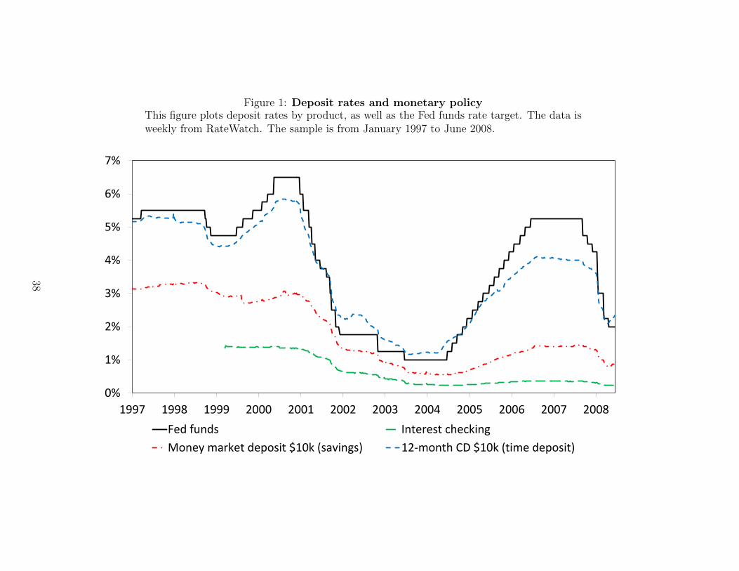
Figure 1: Deposit rates and monetary policyThis figure plots deposit rates by product, as well as the Fed funds rate target. The data isweekly from RateWatch. The sample is from January 1997 to June 2008.

0%

1%

2%

3%

4%

5%

6%

7%

1997 1998 1999 2000 2001 2002 2003 2004 2005 2006 2007 2008

Fed funds Interest checking

Money market deposit $10k (savings) 12-month CD $10k (time deposit)

38

Figure 2: Deposit flows and monetary policyThis figure plots year-over-year changes in savings deposits (Panel A), checking deposits(Panel B), time deposits (Panel C), and total deposits (Panel D) and year-over-changes inthe Fed funds rate. The data are from the Federal Reserve Economic Database (FRED) andthe Flow of Funds. The sample is from January 1986 to June 2008.

Panel A: Savings Deposits

-5%

-4%

-3%

-2%

-1%

0%

1%

2%

3%

4%

-15%

-10%

-5%

0%

5%

10%

15%

20%

25%

30%

1986 1987 1989 1991 1993 1995 1997 1999 2001 2003 2005 2007

Δ F

ed

fu

nd

s ra

te

Δ S

avin

gs d

ep

osi

ts

Savings Deposits Fed funds rate

39

Panel B: Checkable Deposits

-5%

-4%

-3%

-2%

-1%

0%

1%

2%

3%

4%

-15%

-10%

-5%

0%

5%

10%

15%

20%

25%

1986 1987 1989 1991 1993 1995 1997 1999 2001 2003 2005 2007

Δ F

ed

fu

nd

s ra

te

Δ C

he

ckin

g d

ep

osi

ts

Checking deposits Fed Funds rate

40

Panel C: Time Deposits

-5%

-4%

-3%

-2%

-1%

0%

1%

2%

3%

4%

-20%

-15%

-10%

-5%

0%

5%

10%

15%

20%

25%

1986 1987 1989 1991 1993 1995 1997 1999 2001 2003 2005 2007

Δ F

ed

fu

nd

s ra

te

Δ T

ime

de

po

sits

Time deposits Fed funds rate

41

Panel D: Total Deposits

-5%

-4%

-3%

-2%

-1%

0%

1%

2%

3%

4%

-2%

0%

2%

4%

6%

8%

10%

12%

14%

1986 1987 1989 1991 1993 1994 1996 1998 2000 2001 2003 2005 2007

Δ F

ed

fu

nd

s ra

te

Δ T

ota

l de

po

sits

Total deposits Fed funds rate

42

Figure 3: Deposit competitionThis map shows the average Herfindahl index for each county. The Herfindahlis calculated annually using deposit market share by bank and county andaveraged from 1994 to 2008. The data are from the FDIC.

43

Figure 4: Deposit beta and market powerThe figures show the relation between market power and the sensitivity ofdeposit spreads and flows to changes in monetary policy (“deposit beta”) Thefigures are constructed in two steps. The first step is to estimate the followingregression for each county:

∆yijct = α + β∆FFt + εijct.

where yijct is either the change in the deposit spread or deposit growth. This

yields the deposit beta, β, for each county (2751 counties). The second step isrelate deposit betas to market power. We do by sorting counties by Herfindahland averaging deposit betas using 5-percentile intervals (20 points). Panel Ashows the result for 10K money market accounts. Panel B shows the result for12-month certificate of deposits. Panel C shows the result for deposit growth.

Panel A: Savings Deposits

.64

.66

.68

.7.7

2

0 20 40 60 80 100Percentile County Avg. Herfindahl

44

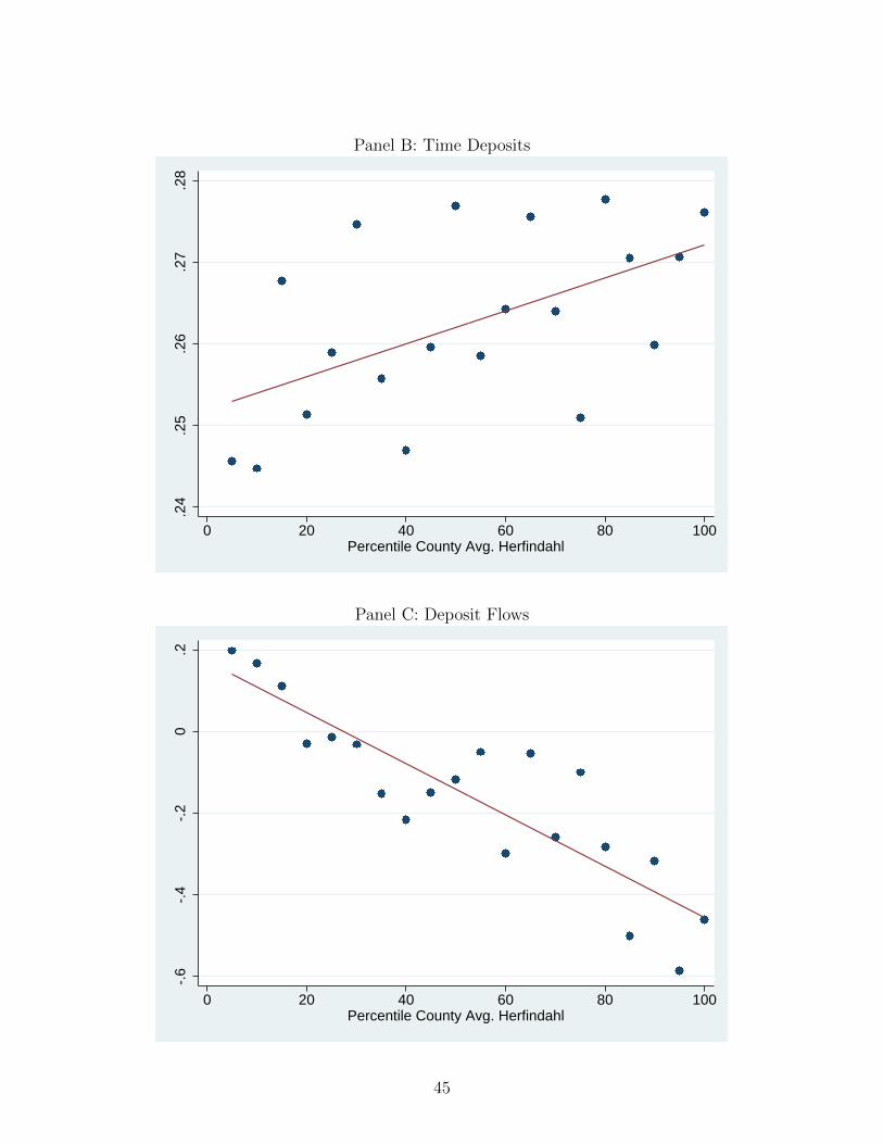
Panel B: Time Deposits

.24

.25

.26

.27

.28

0 20 40 60 80 100Percentile County Avg. Herfindahl

Panel C: Deposit Flows

-.6

-.4

-.2

0.2

0 20 40 60 80 100Percentile County Avg. Herfindahl

45

Figure 5: The price of deposits and market power, event studyThe figure plots the coefficient sum

∑t−5 γτ for t = −5, . . . , 5 weeks, and 95%-

confidence interval, estimated from the regression

∆Spreadijct = αt + βHerfindahlc +5∑

τ=−5

γτHerfindahlc ×∆FFt−τ + εijct.

where ∆Spreadijct is the change in the Fed funds rate minus the change inthe deposit rate on 10K money market accounts over a week. Herfindahl isthe average county-level Herfindahl index calculated based on deposit marketshares by bank. ∆FF is the change in the Fed funds target rate over a week.The sample are all branches in the Ratewatch data from January 1, 1997 toJune 30, 2008. Panel A uses the actual change in the Fed funds target rate;Panel B uses the anticipated change; and Panel C uses the surprise change.These are from Kuttner (2001) and are constructed from Fed funds futures.

Panel A: Total ∆ FF

0.0

5.1

.15

-5 0 5Week

46

Panel B: Anticipated ∆ FF

-.05

0.0

5.1

.15

-5 0 5Week

Panel C: Surprise ∆ FF

0.0

5.1

.15

.2.2

5

-5 0 5Week

47

Table 1: Descriptive statisticsTable 1 provides annual summary statistics at the branch, bank, and county level. Panel A covers county-leveldata for all U.S. counties with at least one branch. The data are from the Census Bureau, Call reports, andthe FDIC. Panel B covers branch-level data for the rate-setting branches. The data are from the FDIC andRatewatch. Panel C covers bank-level data for all U.S. commercial banks. The data are from Call Reports.

Panel A: County characteristics

All Low Herfindahl High HerfindahlMean Median St. Dev. Mean Median St. Dev. Mean Median St. Dev.

Population 91,359 25,113 295,027 151,156 49,889 395,672 31,515 13,496 101,502Area (sq. mi.) 1,055 613 2,483 918 620 1,317 1,193 602 3,252Median h’hold income 36,012 34,349 10,214 38,815 36,953 10,662 33,212 31,889 8,905Poverty rate 14.61 13.60 6.14 13.07 12.40 5.17 16.15 14.90 6.63Unemployment rate 5.44 5.00 2.42 5.15 4.80 2.07 5.74 5.20 2.68Herfindahl 0.354 0.290 0.214 0.204 0.206 0.051 0.503 0.434 0.210

Obs. (county×year) 46,674 23,335 23,329

Panel B: Branch characteristics

All Low Herfindahl High HerfindahlMean Median St. Dev. Mean Median St. Dev. Mean Median St. Dev.

Deposits (mill.) 122 51 830 108 53 402 137 49 1,103Deposit growth 6.19 3.74 18.16 7.06 4.17 19.69 5.33 3.38 16.46Herfindahl 0.239 0.203 0.139 0.146 0.149 0.036 0.332 0.285 0.141MMA 10k spread 1.65 1.66 1.53 1.63 1.64 1.52 1.68 1.68 1.5312-month CD 10k spread -0.07 0.01 0.97 -0.08 0.00 0.97 -0.07 0.02 0.97

Obs. (branch×year) 97,751 48,911 48,840

48

Panel C: Bank characteristics

All Low Herfindahl High HerfindahlMean Median St. Dev. Mean Median St. Dev. Mean Median St. Dev.

Assets (mill.) 765 79 13,817 704 91 9,167 947 81 18,317Herfindahl 0.244 0.212 0.137 0.152 0.157 0.041 0.336 0.291 0.137Deposits spread 1.05 1.24 1.48 1.00 1.19 1.51 1.04 1.24 1.42Assets growth 9.92 6.43 15.70 11.37 7.34 16.77 8.54 5.74 14.04Deposit growth 9.93 5.93 18.17 11.44 6.80 19.51 8.40 5.29 15.93Loan growth 11.81 8.28 19.83 13.47 9.31 21.15 10.14 7.45 17.52Total Deposits/Assets 0.830 0.860 0.113 0.837 0.861 0.095 0.837 0.860 0.091Demand deposits/Assets 0.128 0.117 0.065 0.132 0.119 0.068 0.125 0.117 0.058Savings deposits/Assets 0.199 0.179 0.107 0.217 0.197 0.110 0.186 0.167 0.099Time deposits/Assets 0.391 0.403 0.133 0.383 0.393 0.133 0.405 0.415 0.121Equity/Assets 11.113 9.514 5.945 10.440 9.264 4.568 10.699 9.624 4.310Securities/Assets 25.614 23.910 14.827 24.787 22.972 14.697 26.490 24.806 14.359Loans/Assets 0.602 0.623 0.161 0.617 0.636 0.155 0.603 0.621 0.152Real estate loans/Assets 0.361 0.359 0.170 0.390 0.387 0.168 0.352 0.349 0.162C&I loans/Assets 0.099 0.083 0.071 0.105 0.089 0.073 0.093 0.079 0.065

Obs. (bank×year) 122,821 55,773 55,756

49

Table 2: The price of deposits and market powerThis table examines the effect of monetary policy on the price of deposits (deposit spreads).The sample are banks with two or more rate-setting branches from January 1, 1997 to June30, 2008. ∆ Spread is the change in the deposit spread, which is computed as the change inthe Fed funds target rate minus the change in the deposit rate over a quarter. Herfindahl isthe average county-level Herfindahl index computed from deposit market shares by bank. ∆FF is the change in the Fed funds target rate over a quarter. Panel A reports the results forsavings deposits (10K money market accounts). Panel B reports the results for time deposits(12-month certificate of deposits). Fixed effects are denoted at the bottom of each panel.Standard errors are clustered by county.

Panel A: Savings Deposits∆ Spread

(1) (2) (3) (4)

∆ FF * Herfindahl 0.095** 0.144*** 0.125*** 0.122***(0.040) (0.044) (0.034) (0.036)

Quarter f.e. Y N N NCounty f.e. Y Y Y NState x quarter f.e. N Y Y YBank x quarter f.e. N N Y YBranch f.e. N N N YR2 0.540 0.567 0.804 0.810Observations 87,186 87,186 87,186 87,186

Panel B: Time Deposits∆ Spread

(1) (2) (3) (4)

∆ FF * Herfindahl 0.061** 0.086*** 0.049** 0.050**(0.025) (0.023) (0.019) (0.021)

Quarter f.e. Y N N NCounty f.e. Y Y Y NState x quarter f.e. N Y Y YBank x quarter f.e. N N Y YBranch f.e. N N N YR2 0.357 0.410 0.770 0.776Observations 93,225 93,225 93,225 93,225

50

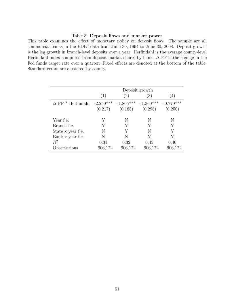
Table 3: Deposit flows and market powerThis table examines the effect of monetary policy on deposit flows. The sample are allcommercial banks in the FDIC data from June 30, 1994 to June 30, 2008. Deposit growthis the log growth in branch-level deposits over a year. Herfindahl is the average county-levelHerfindahl index computed from deposit market shares by bank. ∆ FF is the change in theFed funds target rate over a quarter. Fixed effects are denoted at the bottom of the table.Standard errors are clustered by county.

Deposit growth(1) (2) (3) (4)

∆ FF * Herfindahl -2.250*** -1.805*** -1.360*** -0.779***(0.217) (0.185) (0.298) (0.250)

Year f.e. Y N N NBranch f.e. Y Y Y YState x year f.e. N Y N YBank x year f.e. N N Y YR2 0.31 0.32 0.45 0.46Observations 906,122 906,122 906,122 906,122

51

Table 4: The price of deposits and market power, expected Fed funds changesThis table examines the effect of expected changes in monetary policy on the price of de-posits (deposit spreads). The sample are banks with two or more rate-setting branches fromJanuary 1, 1997 to June 30, 2008. ∆ Spread is the change in the deposit spread, whichis computed as the change in the Fed funds target rate minus the change in the depositrate over a quarter. Herfindahl is the average county-level Herfindahl index computed fromdeposit market shares by bank. ∆ Exp. FF is the expected change in the Fed funds target,which is computed as the difference between the Fed Funds target rate minus the Fed fundsFutures rate three months ahead at the start of a quarter. Panel A reports the results forsavings deposits (10K money market accounts). Panel B reports the results for time deposits(12-month certificate of deposits). Fixed effects are denoted at the bottom of each panel.Standard errors are clustered by county.

Panel A: Savings Deposits∆ Spread

(1) (2) (3) (4)

∆ Exp. FF * Herfindahl 0.152** 0.219*** 0.183*** 0.182***(0.059) (0.064) (0.054) (0.058)

Quarter f.e. Y N N NCounty f.e. Y Y Y NState x quarter f.e. N Y Y YBank x quarter f.e. N N Y YBranch f.e. N N N YR2 0.540 0.567 0.804 0.811Observations 87,186 87,186 87,186 87,186

Panel B: Time Deposits∆ Spread

(1) (2) (3) (4)

∆ Exp. FF * Herfindahl -0.054 -0.023 0.057** 0.056**(0.037) (0.032) (0.026) (0.028)

Quarter f.e. Y N N NCounty f.e. Y Y Y NState x quarter f.e. N Y Y YBank x quarter f.e. N N Y YBranch f.e. N N N YR2 0.357 0.409 0.770 0.776Observations 93,225 93,225 93,225 93,225

52

Table 5: Deposit flows and rate setter’s market powerThis table examines the effect of changes in monetary policy on deposit flows. The sampleare non-rate setting branches that are not located in the same county as their rate settingbranch from June 30, 1994 to June 30, 2008. R.s. Herfindahl is the average county-levelHerfindahl index computed from deposit market shares by bank for the county where therate-setting branch is located. Deposit growth is the log growth rate in branch-level depositsover the year. Fixed effects are denoted at the bottom of the table. Standard errors areclustered by county.

Deposit growth(1) (2) (3) (4)

∆ FF × R.s. Herfindahl -0.980∗∗∗ -1.731∗∗∗ -1.751∗∗∗ -1.707∗∗∗

(0.354) (0.361) (0.537) (0.507)

Year f.e. Y Y N NBranch f.e. N Y N YCounty×year f.e. N N Y YR2 0.006 0.367 0.156 0.473Observations 218,975 218,975 218,975 218,975

53

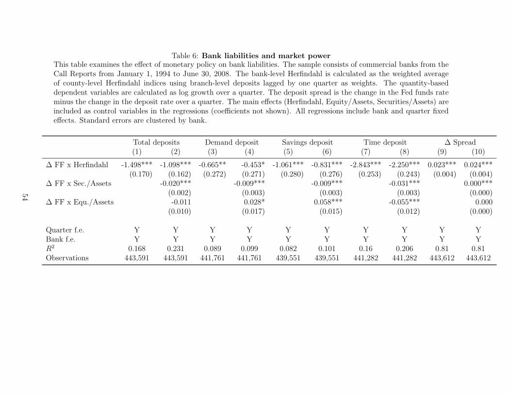
Table 6: Bank liabilities and market powerThis table examines the effect of monetary policy on bank liabilities. The sample consists of commercial banks from theCall Reports from January 1, 1994 to June 30, 2008. The bank-level Herfindahl is calculated as the weighted averageof county-level Herfindahl indices using branch-level deposits lagged by one quarter as weights. The quantity-baseddependent variables are calculated as log growth over a quarter. The deposit spread is the change in the Fed funds rateminus the change in the deposit rate over a quarter. The main effects (Herfindahl, Equity/Assets, Securities/Assets) areincluded as control variables in the regressions (coefficients not shown). All regressions include bank and quarter fixedeffects. Standard errors are clustered by bank.

Total deposits Demand deposit Savings deposit Time deposit ∆ Spread(1) (2) (3) (4) (5) (6) (7) (8) (9) (10)

∆ FF x Herfindahl -1.498*** -1.098*** -0.665** -0.453* -1.061*** -0.831*** -2.843*** -2.250*** 0.023*** 0.024***(0.170) (0.162) (0.272) (0.271) (0.280) (0.276) (0.253) (0.243) (0.004) (0.004)

∆ FF x Sec./Assets -0.020*** -0.009*** -0.009*** -0.031*** 0.000***(0.002) (0.003) (0.003) (0.003) (0.000)

∆ FF x Equ./Assets -0.011 0.028* 0.058*** -0.055*** 0.000(0.010) (0.017) (0.015) (0.012) (0.000)

Quarter f.e. Y Y Y Y Y Y Y Y Y YBank f.e. Y Y Y Y Y Y Y Y Y YR2 0.168 0.231 0.089 0.099 0.082 0.101 0.16 0.206 0.81 0.81Observations 443,591 443,591 441,761 441,761 439,551 439,551 441,282 441,282 443,612 443,612

54

Table 7: Bank lending and market powerThis table examines the effect of monetary policy on bank lending. The sample consists of commercial banks fromthe Call Reports from January 1, 1994 to June 30, 2008. The bank-level Herfindahl is calculated as the weightedaverage of county-level Herfindahl indices using branch-level deposits lagged by one quarter as weights. The quantity-based dependent variables are calculated as log growth over a quarter. The main effects (Herfindahl, Equity/Assets,Securities/Assets) are included as control variables in the regressions (coefficients not shown). All regressions includebank and quarter fixed effects. Standard errors are clustered by bank.

Assets Real Estate Loans C&I Loans Securities(1) (2) (3) (4) (5) (6) (7) (8)

∆ FF x Herfindahl -1.026*** -0.694*** -0.711*** -0.599*** -0.878** -0.717* -0.903** -0.477(0.136) (0.128) (0.229) (0.219) (0.378) (0.374) (0.356) (0.358)

∆ FF x Securities/Assets -0.019*** 0.000 -0.008** -0.014***(0.001) (0.002) (0.004) (0.004)

∆ FF x Equity/Assets -0.01 0.017 0.039** 0.037**(0.007) (0.012) (0.018) (0.016)

Quarter f.e. Y Y Y Y Y Y Y YBank f.e. Y Y Y Y Y Y Y YR2 0.174 0.218 0.168 0.211 0.054 0.069 0.057 0.088Observations 443,748 443,748 439,803 439,803 438,467 438,467 439,322 439,322

55

Table 8: The price of deposits and market power, branch concentrationThis table examines the effect of monetary policy on the price of deposits (deposit spreads).The sample are banks with two or more rate-setting branches from January 1, 1997 to June30, 2008. ∆ Spread is the change in the deposit spread, which is computed as the changein the Fed funds target rate minus the change in the deposit rate over a quarter. Branchherfindahl is the average county-level Herfindahl index computed from deposit market sharesby branch. ∆ FF is the change in the Fed funds target rate over a quarter. Panel A reportsthe results for savings deposits (10K money market accounts). Panel B reports the resultsfor time deposits (12-month certificate of deposits). Fixed effects are denoted at the bottomof each panel. Standard errors are clustered by county.

Panel A: Saving Deposits∆ Spread

(1) (2) (3) (4)

∆ FF × Herfindahl 0.052∗ 0.057∗ 0.073∗∗∗ 0.081∗∗

(0.028) (0.033) (0.027) (0.031)

Branch f.e. N Y N YBank×quarter f.e. Y Y Y YState×quarter f.e. N N Y YR2 0.632 0.648 0.652 0.668Observations 88,481 88,481 88,481 88,481

Panel B: Time Deposits∆ Spread

(1) (2) (3) (4)

∆ FF × Herfindahl 0.050∗∗∗ 0.065∗∗∗ 0.037∗∗ 0.051∗∗

(0.019) (0.022) (0.019) (0.022)

Branch f.e. N Y N YBank×quarter f.e. Y Y Y YState×quarter f.e. N N Y YR2 0.855 0.860 0.863 0.868Observations 91,548 91,548 91,548 91,548

56

Table 9: Deposit flows and market power, branch concentrationThis table examines the effect of monetary policy on deposit flows. The sample are allcommercial banks in the FDIC data from June 30, 1994 to June 30, 2008. Deposit growthis the log growth in branch-level deposits over a year. Herfindahl is the average county-levelHerfindahl index computed from deposit market shares by branch. ∆ FF is the change inthe Fed funds target rate over a quarter. Fixed effects are denoted at the bottom of thetable. Standard errors are clustered by county.

Deposit growth(1) (2) (3) (4)

∆ FF × Herfindahl -1.549∗∗∗ -3.166∗∗∗ -2.008∗∗∗ -1.519∗∗∗

(0.211) (0.224) (0.268) (0.238)

Year f.e. Y Y N NBranch f.e. N Y Y YBank×year f.e. N N Y YState×year f.e. N N N YR2 0.005 0.310 0.428 0.435Observations 873,686 873,686 873,686 873,686

57