the design and statistical analysis of laboratory animal - ccac

1

The design and statistical

analysis of laboratory

animal experiments

Michael FW Festing, Ph.D., D.Sc., CStat.

A workshop held in Quebec, April 2010

[email protected]

2

Replacement

e.g. in-vitro methods, less sentient animals Refinement

e.g. anaesthesia and analgesia, environmental

enrichment Reduction

Research strategy

Controlling variability

Genetics, appropriate model

(disease) Experimental design and statistics

Principles of Humane Experimental

Technique

(Russell and Burch 1959)

3

Survey of statistical quality of

published papers

%

Require statistical revision 61

Serious errors 5

Deficiencies in design 30 (randomisation, size, heterogeneity, bias)

Deficiencies in stat. analysis 45 (sub-optimal methods, errors calculation)

Deficiencies in presentation 33 (omission of data, stats. inappropriate)

McCance, 1995 Aust. Vet. Journal. 72:322

Number of papers studied 133

4

A meta-analysis of 44 randomised

controlled animal studies of fluid

resuscitation

Only 2 said how animals had been allocated

None had sufficient power to detect reliably a halving in risk of death

Substantial scope for bias

Substantial heterogeneity in results, due to method of inducing the bleeding

Odds ratios impossible to interpret

Authors queried whether these animal experiments made any contribution to human medicine

Roberts et al 2002, BMJ 324:474

5

Poor agreement between

animal and human responsesIntervention Human results Animal results (meta-

analysis)

Agree?

Corticosteroids for

head injury

No improvement Improved nurological

outcome

n=17

No

Antofibrinolytics for

surgery

Reduces blood loss Too little good quality data

n=8

No

Thrombolysis with

TPA for acute

ischaemic stroke

Reduces death Reduces death but

publication bias and

overstatement (n=113)

Yes

Tirilazad for stroke Increases risk of death Reduced infarct volume and

improved behavioural score

n=18

No

Corticosteroids for

premature birth

Reduces mortality Reduces mortality n=56 Yes

Bisphosphonates

for osteoperosis

Increase bone density Increase bone density n=16 Yes

Perel et al (2007) BMJ 334:197-200

6

Survey of 271 papers. Results

published in PLoS One

Of the papers studied:

5% did not clearly state the purpose of the study

6% did not indicate how many separate experiments were done

13% did not identify the experimental unit

26% failed to state the sex of the animals

24% reported neither age not weight of animals

4% did not mention the number of animals used

0% justified the sample sizes used

35% which reported numbers used these differed in the materials and methods and the results sections

etc.

Kilkenny et al (2009), PLoS One Vol. 4, e7824

7

Scientific papers should give sufficient detail

so that the experiment(s) can be repeated

The objectives of the research and/or the hypotheses to be tested

The reason for choosing the particular animal model

The species, strain, sex, age/weight, source and type of animal used and brief details of environment, diet and husbandry

Each experiment should be numbered giving details of Purpose of the experiment

The experimental design

Completely randomised, randomised block, factorial design etc.

The “experimental unit”

Method of randomisation and whether blinding was used (where appropriate)

Method of sample size determination and number of animals used

The statistical methods used for analysis

Conclusions

Over-all conclusions

8

Types of experiment

Pilot study Logistics and preliminary information

Exploratory experiment Aim is to provide data to generate hypotheses

May “work” or “not work”

Often many outcomes

Statistical analysis may be problematical (many characters measured, data snooping). p-values may not be correct

Confirmatory experiment Formal hypothesis stated a priori. p-values should be

correct

9

A well designed experiment

Absence of bias Experimental unit, randomisation, blinding

High power Low noise (uniform material, blocking, covariance)

High signal (sensitive subjects, high dose)

Large sample size

Wide range of applicability Replicate over other factors (e.g. sex, strain): factorial

designs

Simplicity

Amenable to a statistical analysis

10

Experimental unit

Smallest division of the experimental

material such that any two experimental

units can receive different treatments

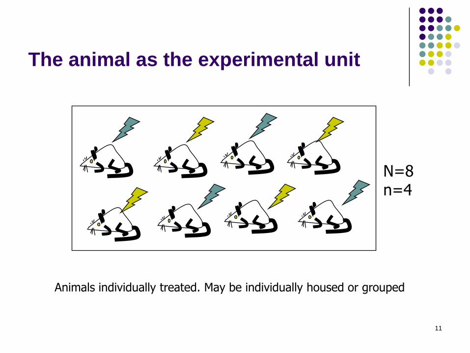
11

The animal as the experimental unit

Animals individually treated. May be individually housed or grouped

N=8n=4

12

A cage/room as the

experimental Unit.

Treatment in water/diet, animals/group, environmental enrichment etc.

N=4n=2

Treated TreatedControl Control

13

A tank of fish as the

experimental unit

N=2n=1

14

An animal for a period of time: repeated

measures or crossover design

Animal

1

2

3

Treatment 1

Treatment 2

N

4

4

4

N=12n= 6

15

Teratology: mother treated,

young measured

Mother is the experimental unit.

N=2n=1

16

Failure to identify the experimental unit

correctly (aim to look at strain

differences in diurnal pattern of blood

alcohol)

ELD groupELD group

Single cage of 8 mice killed at each time point (288 mice in total)

17

Experimental units

An investigator takes a rat at random and

injects it with a test compound

He takes another rat at random as a control

and injects it with the vehicle

Both rats are weighed once per week for 10

weeks,

The investigator then does a t-test to

compare these weights.

18

The experimentWeek Control.rat Treated.rat

1 120 121

2 122 122

3 120 120

4 125 125

5 127 120

6 127 119

7 129 118

8 130 117

9 132 118

10 131 120

p-value = 0.001

The treated rat weighs significantly less (p<0.05) than the control rat.

He concludes that the treatment significantly reduced body weight.

What is wrong with this experiment?

19

Experimental units must be

randomised to treatments

Physical: numbers on cards. Shuffle and take

one

Tables of random numbers in most text

books

Use computer. e.g. EXCEL or a statistical

package such as MINITAB

20

Randomisation

Original Randomised1 21 31 31 12 22 12 22 13 33 23 33 1

2 3 3 1 etc individually housed

2,X 3,X 3,X etc individual + companion

2,3,3,1 2,1,2,1 etc Grouped at random

1, 2, 3 1, 2, 3 etc Randomised block

1,1,1,1,1 2,2,2,2 etc By treatment

How should the animals be caged?

1, 1 1, 1 2, 2 2, 2 etc (but cage is EU)

21

Failure to randomise and/or blind

leads to more “positive” results

Blind/not blind odds ratio 3.4 (95% CI 1.7-6.9)

Random/not random odds ratio 3.2 (95% CI 1.3-7.7)

Blind Random/ odds ratio 5.2 (95% CI 2.0-13.5)not blind random

290 animal studies scored for blinding, randomisation and positive/negative outcome, as defined by authors

Babasta et al 2003 Acad. emerg. med. 10:684-687

22

Some factors (e.g. strain, sex) can not be randomised

so special care is needed to ensure comparability

Outbred TO (8-12 weeks

commercial)

Inbred CBA (12-16

weeks Home bred)

Six cages of 7-9 mice of each strain: error bars are SEMs

"CBA mice showed greater

variability in body weights than

TO mice..."

23





Large sample size


designs

Simplicity


24

Genetic Stocks of Laboratory

Animals

Outbred stocks

e.g. Swiss mice, Wistar Rats Inbred strains

e.g. BALB/c, F344Mutants and polymorphisms

e.g. Foxn1nu, Foxn1rnu

Transgenic strains

e.g. TG.AC, BigBlue

25

Exercise 1A

You have developed a compound which you think will help to

prevent rejection of transplanted hearts, and you want to test

this experimentally.

The experiment will involve heart grafts between a donor and

recipient rat (whose own heart is not removed) with a control

group and one treated with the compound.

The following rat strains are available: Outbred Wistar and

Sprague-Dawley and inbred ACI, F344 and LEW.

Which strains will you use as donor and recipient, and why?

26

Exercise 1B

You know it is not acutely toxic but need to do a long-term

toxicity study with control and treated rats.

You discuss this with a toxicologst who points out that you wish

to model humans who are genetically heterogeneous. He

suggests that you use outbred genetically heterogeneous

Sprague-Dawley rats, the strategy used by virtually all

toxicologists.

Do you decide to accept or reject his advice. Give your reasons

27

Exercises 1A and 1B

1A. Heart transplant. Choose donor and recipient rats

from:

Outbred: Wistar, Sprague-Dawley,

Inbred: ACI, LEW, F344

Question B is the compound chronically toxic?

1B. Toxicity test. Aim is to model humans. Outbred

Sprague-Dawley rats suggested. Accept or reject this

advice?

Question A: does your new drug prolong graft

survival?

28

Variable results with heart

transplants

"We transplanted hearts of young ... Fishers into ...

recipient Sprague-Dawleys. An outbred strain was

selected since such animals are usually heartier

and easier to handle...

We are puzzled by our results....palpable heart

beats were evident in the saline group long after

acute rejections...were expected...Results in the

experimental groups varied considerably..."

29

Choice of outbred stocks

"..it is more correct to test on a random-bred

stock on the grounds that it is more likely that at

least a few individuals will respond to the

administration of an active agent in a group which

is genetically heterogeneous"

Arcos JC, Argus MF, Wolf G, eds. (1968) Chemical

induction of cancer. 491pp, London, Academic Press.

30

Control Treated

Beagle Goat

Chicken Pig

Mouse Crow

Horse Frog

Gerbil Hamster

Guinea-pig Quail

Lion Beaver

Duck Cat

The problem with genetic heterogeneity

A “completely randomised” design

31

A randomised block design

Control Treated

Beagle Beagle

Mouse Mouse

Horse Horse

Gerbil Gerbil

Guinea-pig Guinea-pig

Lion Lion

Duck Duck

Rabbit Rabbit

32

A better design (randomised

block)

Control Treated

A/J A/J

A2G A2G

BALB/c BALB/c

CBA CBA

C3H C3H

C57BL/6 C57BL/6

DBA/2 DBA/2

NIH NIH

33

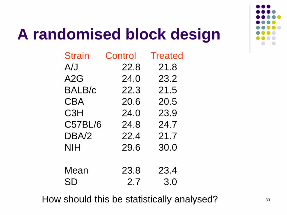
A randomised block design

Strain Control Treated

A/J 22.8 21.8

A2G 24.0 23.2

BALB/c 22.3 21.5

CBA 20.6 20.5

C3H 24.0 23.9

C57BL/6 24.8 24.7

DBA/2 22.4 21.7

NIH 29.6 30.0

Mean 23.8 23.4

SD 2.7 3.0

How should this be statistically analysed?

34

Statistical analysisStrain Control Treated Control-treated

A/J 22.8 21.8 1.0

A2G 24.0 23.2 0.8

BALB/c 22.3 21.5 0.8

CBA 20.6 20.5 0.1

C3H 24.0 23.9 0.1

C57BL/6 24.8 24.7 0.1

DBA/2 22.4 21.7 0.7

NIH 29.6 30.0 -0.4

Mean 23.8 23.4 0.4

SD 2.7 3.0 0.5

35

Paired t-test

One-Sample T: Difference

Test of mu = 0 vs mu not = 0

Variable N Mean StDev SE Mean

Difference 8 0.387 0.482 0.171

Variable 95.0% CI T P

Difference ( -0.017, 0.791) 2.27 0.058

36

Two-way ANOVA without interaction

for a randomised block design

Analysis of Variance for Weight

Source DF SS MS F P

Strains 7 111.717 15.960 137.18 0.000

Treatmen 1 0.599 0.599 5.15 0.058

Error 7 0.814 0.116

Total 15 113.131

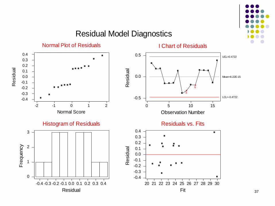
37

-0.4 -0.3 -0.2 -0.1 0.0 0.1 0.2 0.3 0.4

0

1

2

3

Residual

Fre

quency

Histogram of Residuals

0 5 10 15

-0.5

0.0

0.5

Observation Number

Resid

ual

I Chart of Residuals

5

6

Mean=6.22E-15

UCL=0.4722

LCL=-0.4722

20 21 22 23 24 25 26 27 28 29 30

-0.4

-0.3

-0.2

-0.1

0.0

0.1

0.2

0.3

0.4

Fit

Resid

ual

Residuals vs. Fits

-2 -1 0 1 2

-0.4

-0.3

-0.2

-0.1

0.0

0.1

0.2

0.3

0.4

Normal Plot of Residuals

Normal Score

Re

sid

ual

Residual Model Diagnostics

38

Statistical analysis should fit

the purpose of the studyA Completely Randomised Design

Experimental unit??

Lesion diameter clearly increases with power, but aim is to quantify this

Lesion diameter following microwave treatment of pig liver

Power

(watts) Mean

50 3.3 3.2 2.8 2.8 2.4 2.7 3.2 3.8 1.5 2.9

100 4.7 4.0 3.5 4.4 3.9 4.8 4.4 3.7 4.0 4.2

150 5.5 5.0 4.4 4.5 6.0 6.5 5.0 5.0 5.3

200 5.8 6.0 5.9

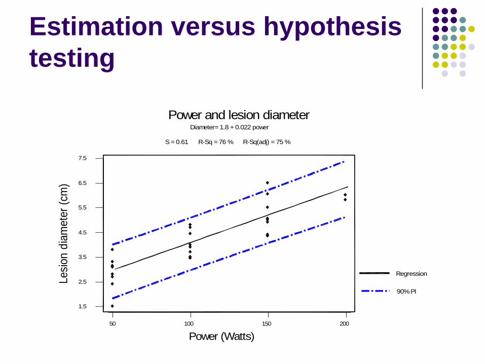
39

50 100 150 200

1.5

2.5

3.5

4.5

5.5

6.5

7.5

Power (Watts)

Lesi

on

dia

mete

r (c

m)

Diameter= 1.8 + 0.022 power

S = 0.61 R-Sq = 76 % R-Sq(adj) = 75 %

Regression

90% PI

Power and lesion diameter

Estimation versus hypothesis

testing

40

Sample size

Tradition and experience

Power analysis

The Resource Equation

41

Power Analysis for sample size and

effects of variation

A mathematical relationship between six variables

Needs subjective estimate of effect size to be detected (signal)

Needs an estimate of the SD (for measurement characters)

Has to be done separately for each character

Not easy to apply to complex designs

Essential for expensive, simple, large experiments (clinical trials)

Useful for exploring effect of variabilityA second method “The Resource Equation” is described later

42

Power analysis: the variables

Sample size

Signala) Effect size of scientific interest

or b) actual response

Chance of a false positive result. Significance level

(0.05)

Sidedness of statistical test (usually 2-sided)

Power of theExperiment (80-90%?)

NoiseVariability of the

experimental material

43

Comparison of two anaesthetics for dogs

under clinical conditions (Vet. Anaesthes. Analges.)

Unsexed healthy clinic dogs,• Weight 3.8 to 42.6 kg. • Systolic BP 141 (SD 36) mm Hg

Assume: • a 20 mmHg difference between groups is of clinical importance, • a significance level of a=0.05• a power=90%• a 2-sided t-test

Signal/Noise ratio 20/36 = 0.56(standardised effect size)

d = |m1-m2|/s

Required sample size 68/group

44

Power and sample size

calculations using nQuery Advisor

45

A second paper described:

• Male Beagles weight 17-23 kg• mean BP 108 (SD 9) mm Hg.• Want to detect 20mm difference between groups (as before)

With the same assumptions as previous slide:

Signal/noise ratio = 20/9 = 2.22

Required sample size 6/group

46

Summary for two sources of dogs: aim is to

be able to detect a 20mmHg change in blood

pressure

Type of dog SDev Signal/noise Sample %Power (n=8) size/gp(1) (2)

Random dogs 36 0.56 68 18Male beagles 9 2.22 6 98

(1) Sample size: 90% power(2) Power, Sample size 8/group

Assumes a=5%, 2-sided t-test and effect size 20mmHg

What should the investigator do?

47

Group size and Signal/noise

ratio

0

20

40

60

80

100

120

140

0 0.5 1 1.5 2 2.5 3

Effect size (Std. Devs.)

Gro

up

siz

e

90%

80%

Assuming 2-sample, 2 sided t-test and 5% significance level

Signal/noise ratio

Power

Neutral

Bad

Good

48

35 45 55

Weight

Body weight of mice housed 1, 2, 4 or 8 per cage

Mice/cage

1 SD=5.8

2 SD=3.9

4 SD=3.2

8 SD=2.9

Chvedoff et al (1980) Arch.Toxicol. Suppl 4:435

49

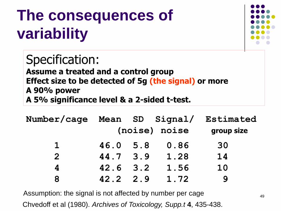
Specification: Assume a treated and a control group Effect size to be detected of 5g (the signal) or moreA 90% powerA 5% significance level & a 2-sided t-test.

The consequences of

variability

Number/cage Mean SD Signal/ Estimated

(noise) noise group size

1 46.0 5.8 0.86 30

2 44.7 3.9 1.28 14

4 42.6 3.2 1.56 10

8 42.2 2.9 1.72 9

Assumption: the signal is not affected by number per cage

Chvedoff et al (1980). Archives of Toxicology, Supp.t 4, 435-438.

50

Variation in kidney weight in

58 groups of rats

0

10

20

30

40

50

60

70

80

90

1 5 9 13 17 21 25 29 33 37 41 45 49 53 57

Sample number

Va

ria

bil

ity Mycoplasma

Outbred

F1

F2

Gartner,K. (1990), Laboratory Animals, 24:71-77.

51

Required sample sizes

Factor Type Std.Dev Signal/

noise*

Sample

size

Power**

Genetics F1 hybrid 13.5 1.48 10 87

F2 hybrid 18.4 1.09 15 63

Outbred 20.1 0.99 18 55

Disease Mycoplasma

free

18.6 1.08 15 53

With

Mycoplasma

43.3 0.23 76 14

*signal is 20 units, two sided t-test, a=0.05, power = 80%** Assuming fixed sample size of 10/group

Aim: to detect a difference in kidney weight of 20%

52

A fundamental rule

“Good experiments minimize random

variation, so that any variation due the

factors of interest can be detected more

easily.”

Ruxton and Colgrave 2003 Experimental design for the life sciences,

2nd. edition, p6.

53

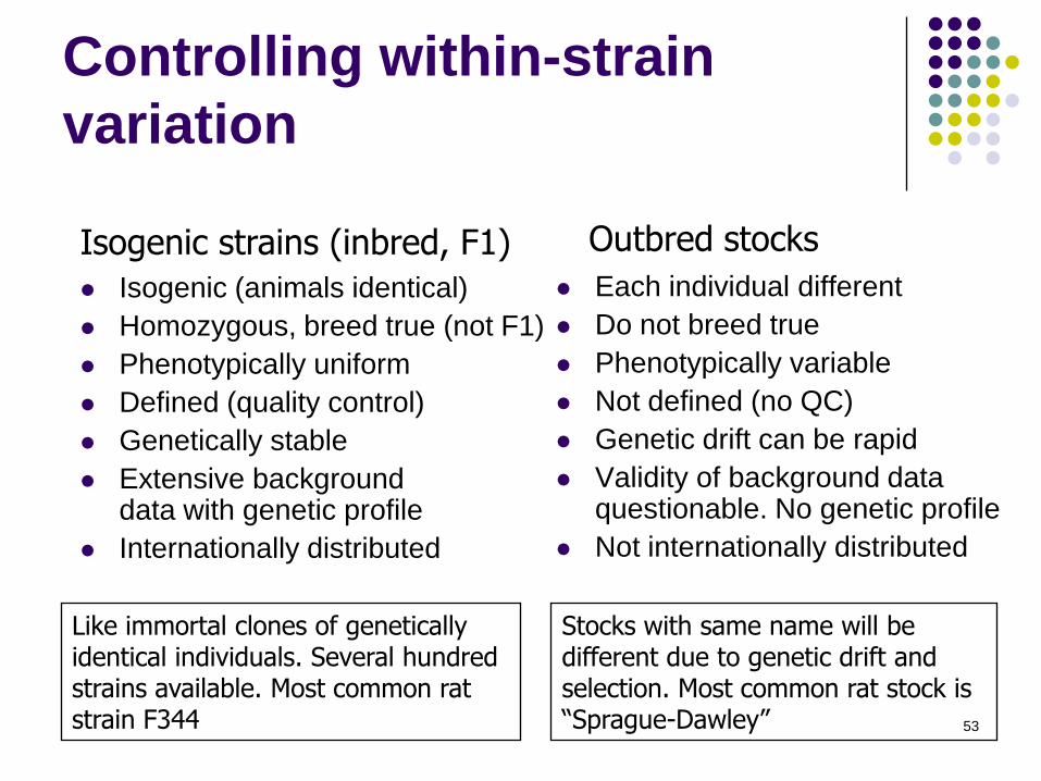
Controlling within-strain

variation

Isogenic (animals identical)

Homozygous, breed true (not F1)

Phenotypically uniform

Defined (quality control)

Genetically stable

Extensive backgrounddata with genetic profile

Internationally distributed

Each individual different

Do not breed true

Phenotypically variable

Not defined (no QC)

Genetic drift can be rapid

Validity of background data questionable. No genetic profile

Not internationally distributed

Isogenic strains (inbred, F1) Outbred stocks

Like immortal clones of genetically identical individuals. Several hundred strains available. Most common rat strain F344

Stocks with same name will be different due to genetic drift and selection. Most common rat stock is “Sprague-Dawley”

54

Isogenicity & Identifiability

55

Genetic contamination of MRL

mice

56

No easy quality control with

outbred stocks

57

Genetics is important: Twenty two Nobel Prizes since 1960

for work depending on inbred strains

Cancer

mmTV

Transmissable

encephalopathacies/prions

Pruisner

Retroviruses, Oncogenes & growth factors

Cohen, Levi-montalcini, Varmus, Bishop, Baltimore, Temin

Humoral immunity/antibodies

T-cell receptor

Tonegawa, Jerne

Cell mediated immunity

Immunological tolerance

H2 restriction, immune responses

Medawar, Burnet, Doherty, Zinkanagel

Benacerraf (G.pigs)

Genetics

Snell C.C. Little, DBA, 1909

Inbred Strains and derivatives

Jackson Laboratory

monoclonal antibodies

BALB/c mice

Kohler and Millstein

SmellAxel & Buck

ES cells & “knockouts”Evans, Capecchi, Smithies

58

Why do scientists continue to use outbred

stocks when inbred strains are available?

Humans are outbred

We wish to model humans

Therefore we should use outbred animals

59

Why do scientists continue to use outbred

stocks when inbred strains are available?

Humans weigh 70 kg

We wish to model humans

Therefore we should use 70 kg animals

60

Models and the high fidelity fallacy

Fidelity

Ability to discriminate

Cindy doll

Home pregnancy kit

NH primate

In-vitro test

(After Russell and Burch 1959)

Outbred rat

Inbred rat

61

Models: a two-step process

Is the model a good model of humans (or

other target species)? This is decided a priori

How does the model respond to the

intervention?

62

Mammary tumoursIn mouse strain C3H-A

Location % Age (m)

USA 100 6.8

Australia 10 7.7

vy

Sabine,J.R et al (1973). Spontaneous tumours in C3H-Avy and C3H-AvyfB mice: High incidence in the United States and low incidence in Australia. Journal of the National Cancer Institute 50, 1237-1242.

63

The randomised block design: another

method of controlling noise

B C A

A C B

B A C

A C B

B C A B1

B2

B3

B4

B5

Treaments A, B & C

• Randomisation is within-block• Can be multiple differences

between blocks• Heterogeneous age/weight• Different shelves/rooms• Natural structure (litters)• Split experiment in time

64

A randomised block

experiment

0

50

100

150

200

250

300

350

400

450

500

1 2 3

Week

Ap

op

tosis

sco

re

Control

CGP

STAU

365 398 421 423 432 459 308 320 329

Treatment effect p=0.023(2-way ANOVA)

65

Randomised BlocK ANOVA

Correct 2-way Analysis of Variance for Apop

Source DF SS MS F P

Block 2 21764 10882 114.82 0.000

Treat 2 2129 1064 11.23 0.023

Error 4 379 94

Total 8 24272

Incorrect One-Way Analysis of Variance

Analysis of Variance for Apop

Source DF SS MS F P

Treat 2 2130 1065 0.29 0.759

Error 6 22143 3691

Total 8 24273

66

-10.0 -7.5 -5.0 -2.5 0.0 2.5 5.0 7.5

0

1

2

3

Residual

Fre

quency


0 1 2 3 4 5 6 7 8 9

-20

-10

0

10

20

Observation Number

Resid

ual


Mean=3.16E-14

UCL=20.17

LCL=-20.17

300 350 400 450

-10

0

10

Fit

Resid

ual

Residuals vs. Fits

-1.5 -1.0 -0.5 0.0 0.5 1.0 1.5

-10

0

10


Normal Score

Re

sid

ual


67

The Resource Equation. Another method

of determining sample size:

Depends on the law of diminishing returns

Simple. No subjective parameters

Useful for complex designs and/or multiple outcomes

Does not require estimate of Standard Deviation

Crude compared with Power Analysis

Does not work for proportions

E= (Total number of animals)-(number of treatment groups)

10<E<20 (but give some tolerance)

Mead,R. The design of experiments. (Cambridge University Press, 1988).

68

The resource equation method

0

2

4

6

8

10

12

1 3 5 7 9 11 13 15 17 19 21 23 25 27 29

Degrees of freedom (E)

Info

rmat

ion

Degrees of freedom (E)

Info

rmation

E=(total number of animals)-(number of treatment groups)

E=10 E=20

69

C T1 T2 T3

The Resource Equation

With completely randomised design:

E= (total number) – (no treatments)

24 - 4 = 20

70

A factorial design incorrectly analysed as four

separate experiments

n=8 mice per group, 8 treatment gps, 64 mice total. E=56

AlternativeA 2*4 factorial design with3 mice per group:E=24-8 = 16

Saving:40 miceFormal test of interaction

71





Large sample size


designs

Simplicity


72

Factorial designs

Single factor design

Treated Control

E=16-2 = 14

One variable at a time (OVAT)

Treated ControlTreated Control

E=16-2 = 14 E=16-2 = 14

Factorial design

Treated Control

E=16-4 = 12

73

Factorial designs

(By using a factorial design)”.... an experimental investigation, at the same time as it is made more comprehensive, may also be made more efficient if by more efficient we mean that more knowledge and a higher degree of precision are obtainable by the same number of observations.”

R.A. Fisher, 1960

74

A 3(treatments)x3 (ages)

factorial (but unequal numbers)

75

2 (strains) x 3 (treatments) x 6(times)

= 36 treatment combinations factorial

(but wrong experimental unit)

ELD

group

ELD

group

As designed with 8/group: N= 288 T= 36 E = 222 (assuming correct housing)Say 2/gp N= 72, T=36 E=36, saving of 182 mice

76

Factorial: what do we mean by

group size?

Trt. Ctrl.

Single factorInbred strain

Trt. Ctrl.

2x2 Factorial

Trt. Ctrl. Trt. Ctrl.

2x4 Factorial Randomised block

Trt. Ctrl.

Outbred

8 8 or 4? 8 or 2? 8 or 1? 8 or ??

77

Comparison: single outbred stock

vs factorial with inbred strains

500 1000 1500 2000 2500

CD-1 8 8 8 8 8 8

CBA 2 2 2 2 2

C3H 2 2 2 2 2

BALB/c 2 2 2 2 2

C57BL 2 2 2 2 2

2

2

2

2

Inbred

0

Outbred

Dose of chloramphenicol (mg/kg)

Festing,M.F.W.,et. al. (2001) Strain differences in haematological response to chloramphenicol succinate in mice: implications for toxicological research. Food and Chemical Toxicology, 39, 375-383.

78

Red blood cell counts

Strain Control 1500mg/kgCBA 10.57 8.33CBA 9.88 8.51C3H 8.49 7.40C3H 7.87 7.51BALB/c 10.10 8.95BALB/c 10.08 9.29C57BL 9.60 9.81C57BL 9.56 9.83

CD-1 9.10 8.90CD-1 10.27 8.26CD-1 9.01 7.45CD-1 7.76 8.50CD-1 8.42 8.71CD-1 8.83 7.79CD-1 10.01 8.67CD-1 8.65 8.19

Four inbred strains

One outbred stock

79

Signal Noise

Strain N 0 1500 (Difference) (SD) Signal/noise p

BALB/c 4 10.09 9.12 0.97 0.25 3.88

C3H 4 8.18 7.46 0.72 0.25 2.88

C57BL 4 9.58 9.82 (0.24) 0.25 (0.96)

CBA 4 10.23 8.42 1.81 0.25 7.24

Mean 16 9.51 8.70 0.81 0.25 3.24 <0.001

Dose * strain <0.001

Counts following chloramphenicol at

1500mg/kg

Signal Noise


CD-1 16 9.01 8.31 0.70 0.68 1.03 0.058

Signal Noise


CD-1 16 9.01 8.31 0.70 0.68 1.03 0.058

Red blood cell counts

Signal Noise


CD-1 16 9.01 8.31 0.70 0.68 1.03 0.058

80

Signal Noise


CBA 4 2.25 0.30 1.95 0.34 5.73

C3H 4 2.15 0.40 1.85 0.34 5.44

BALB/c 4 1.05 1.35 (-0.30) 0.34 (-0.88)

C57BL 4 2.25 0.95 1.30 0.34 3.82

Mean 16 1.93 1.20 0.73 0.34 2.15 <0.001

Dose * strain <0.001

WBC counts following chloramphenicol at

2500mg/kg

Signal Noise


CD-1 16 2.23 1.83 0.40 0.86 0.47 0.38

White blood cell counts

81

A factorial randomised block

experiment to detect the effect of BHA

on liver EROD activity

Block 1

Treated Control

Block 2

Treated Control

The two blocks were separated by approximately 3 months

A/J

129/Ola

NIH

BALB/c

82

A real experiment to detect the effect of

BHA on liver EROD activity

Block 1

Treated Control

Block 2

Treated Control

The two blocks were separated by approximately 3 months

A/J

129/Ola

NIH

BALB/c

7.7

8.4

9.8

9.7

18.7

17.9

19.2

26.3

6.4

6.7

8.1

6.0

16.7

14.4

12.0

19.8Mean14.7

Mean11.3 (diff 3.4)

83

-2.0 -1.5 -1.0 -0.5 0.0 0.5 1.0 1.5 2.0

0

1

2

3

4

Residual

Fre

quency


0 5 10 15

-3

-2

-1

0

1

2

3

Observation Number

Resid

ual


Mean=1.72E-15

UCL=2.5

LCL=-2.5

5 15 25

-2

-1

0

1

2

Fit

Resid

ual

Residuals vs. Fits

-2 -1 0 1 2

-2

-1

0

1

2


Normal Score

Re

sid

ual


84

Analysis of Variance for EROD

Source DF SS MS F P

Block 1 47.610 47.610 18.37 0.004

Strain 3 32.963 10.988 4.24 0.053

Treatmen 1 422.303 422.303 162.96 0.000

Strain*Treatmen 3 40.342 13.447 5.19 0.034

Error 7 18.140 2.591

Total 15 561.358

85

Effects of BHA on liver EROD activity in four mouse strains (a 2x4

factorial randomised block experiment)

2 mice per mean (16 total), done as a randomised block design.

A/J 129/Ola NIH BALB/c A/J 129/Ola NIH BALB/c

0

5

10

15

20

25EROD activity

Control BHA

Treatment p<0.001

Strain p=0.05

Strain x Treatment, p=0.03

Std. Dev. 1.6

86

Conclusions

There is evidence that animal experiments are not always well designed

Five requirements for a good design Unbiased (randomisation, blinding)

Powerful (control variability)

Wide range of applicability (factorial designs, common but frequently analysed incorrectly)

Simple

Amenable to statistical analysis

Better training

More consultant statisticians

the design and statistical analysis of laboratory animal - ccac

Documents