the development of demand elasticity model for demand
TRANSCRIPT

The Development of Demand Elasticity Model for
Demand Response in the Retail Market Environment
M. Babar, P.H. Nguyen, V. Cuk, I.G. Kamphuis
Eindhoven University of Technology, Department of Electrical Engineering,
Electrical Energy Systems, 5600 MB, Eindhoven, the Netherlands,
Abstract—In the context of liberalized energy market, increasein distributed generation, storage and demand response hasexpanded the price elasticity of demand, thus causing the additionof uncertainty to the supply-demand chain of power system.In order to cope with the challenges of demand uncertaintyunder the unbundled electricity market, the concept of Market-based Control Mechanism (MCM) in retail market environmenthas been emerging. This paper presents the concept consideringdemand elasticity as an opportunity in retail market environmentfor inventing a new bid mechanism. This work formulates demandelasticity model as a Markov decision problem and implementspursuit algorithm as a machine learning technique to evaluatethe price elasticity of demand by predicting the price. Theperformance of the algorithm is compared with the numericalcalculation of price elasticity of demand for the given simulationsettings.
Keywords—Demand Response, Demand Elasticity, ElectricityMarket, Pursuit Algorithm.
I. INTRODUCTION
For the last two decades, power system has been restruc-tured and deregulated around Europe [1]. This change dividesthe vertical integrated systems into multiple independent stake-holders including generation companies, transmission compa-nies, distribution companies and retail companies (energy sup-pliers). Economic theory also states that disintegration of elec-tricity market creates distributed and transparent competitionamong the new smaller players, thus resulting in differentiatedservice offerings, lower prices, and the enhancement of marketefficiency [2]. Moreover, it is also seen in many EU memberstates that retail market environment after the liberalization ofelectricity market has established the transparent competitionin electricity market players as the consumer can select theenergy supplier of its own choice. Thus, it is also argued thatthe dynamic pricing would be a powerful way to encourageconsumers to behave in an economically optimal way.
Concurrently, the concept of demand dispatch has in-troduced the demand elasticity as an economic opportunityfor the retail market participant (i.e. retailer or energy ser-vice provider), thus encouraging them to implement DemandResponse (DR) programs. Although ICT infrastructures areadvanced enough to implement DR programs in mass atdifferent levels of the grid, there are still many challenges tocope before making the DR a reality [3]. Recently, many DRprograms have been designed and implemented for differentmarket mechanisms to reduce the peak demand or shift demandfrom peak to off-peak periods.
Authors in [4]–[6] present a market-based control mech-anism (MCM) in which the DR of domestic consumers istraded as commodity in retail market. In [4], it is presentedthat the distributed control of time shifting-loads over pricesignals optimizes the resource allocation by considering theirconstraints (i.e. temperature, cycling power etc.) with an aimto minimize the total energy cost. Similarly, EnerNOC hasused a methodology of energy bidding for large consumers[5]. Herein, the organization calls the participating consumerto reduce the power available at their disposal during thegiven time period. In the exchange of this service, incentivepayments are paid to the consumer according to the market-price. Ref. [7] reports that the incentive-based load controlmechanisms has already been implemented over consumer’sthermal appliances. Similarly, a platform has been developedin [8] for the commercial or large consumer which enablesthem to manage their bid online.
Ref. [6], [9] share the implementation of MCM by usingmulti agent systems, where each downstream agent commu-nicates a bid as function of demand to the upstream agent.In response, the downstream agent gets a price to act ac-cordingly. One of the interesting features of this approach isthe consideration of the demand elasticity as a commodity,and it is transacted in the retail market via a bid even bythe domestic consumer. The consumer that takes part in thisprogram is usually referred as an active consumer. Furthermorethe retailer generates incentive price to utilize the availabledemand flexibility provided by the active consumer. Henceif the consumer’s bid is accepted, then it is paid by theincentive payment. Currently one of the challenges in the retailmarket DR program is to anticipate and integrate the demandelasticity in the bidding mechanism because existing demand-side bidding mechanisms have already been facing such issues[10].
Although the concept of demand elasticity model (DEM)has been proposed for DR estimation in late 90s, it has notbeen applied in any bidding mechanism for retail marketenvironment so far [10]–[12]. Verily one of the main reason isthat the unbundling of the electricity market took place duringthe last decade creating new opportunities and challenges forthe retail market. Secondly, the fast electrification and theintroduction of distributed generation have already made andwould make the demand much elastic than before. Thirdly, theintroduction of smart metering and ICT advances have enabledthe domestic consumer to bid easily against the energy at itsdisposal. That is why, in this paper the concept of DEM ispresented for MCM which would help in the development of

{{
Dev
ice
Envi
ron
men
tA
gen
t
Energy Market
Participants
AbstractionLayer
EnergyApplication
ResourceLayer
BidPrice
Fig. 1. FlexiblePower Application Infrastructure
future bidding mechanisms. Moreover, this paper formulatesthe problem in the consideration of a platform named Flex-iblePower Application Infrastructure (FPAI) which has beenrecently developed by Flexiblepower Alliance Network (FAN).The high level overview of the FPAI is shown in Fig. 1.FPAI is an open framework which has been developed withan objective to find the integrated approach towards the futuregird [13].
Referring to the same platform, the Energy Application(EA) has aggregated demand of the consumer and the informa-tion of demand elasticity and with this the EA has to managethe bid. Hence, the value proposition by the customer to amarket participant in form of demand elasticity is formulatedin section II. The problem is modeled in section III whichdevelops the concept of demand elasticity matrix and discussesthe algorithm that learns the consumer behavior using amachine learning technique. Section IV presents the simulationresults and Section V concludes the paper.
II. PROBLEM FORMULATION
Consider T is the timeframe of the electricity retail marketsuch that T = {t1, t2, . . . , ti, . . . , tI} which is divided intoI equal intervals, then during the entire timeframe T thedemand elasticity could be treated as commodity that couldbe substituted or complemented with each other. Therefore,the price elasticity of demand or demand elasticity is definedas the change in demand ∂Di at the given hour ti due to thechange in the electricity price ∂Pi during the same hour aswell as other hours {tj ∈ T : i 6= j}. Mathematically
ε =
∂Di
do
∂Pi
po
(1)
Where ε is the elasticity coefficient which indicates thelevel of DR due to the change in price, do is initial demandvalue, po is initial price. However the calculation of the
point elasticity as shown in (1) requires functional relation-ship between the demand and the price, and can only becalculated wherever the function is defined. In addition, theprice elasticity of electricity demand at domestic level couldnot be generalized by any specific function. Nevertheless, R.Allen presents the concept of arc elasticity of demand wherethe percentage change could be calculated relative to the mid-point [14]. In this way, the calculated demand elasticity wouldbe (a) symmetric with respect to change in the price and thedemand, (b) independent from the calculation of functionalrelationship and (c) equal to unity if the total revenue at bothpoints are similar. Thus, the normalized demand elasticity isdenoted as:
εii =∂Di
∂Pi
×pi+pi−1
2di+di−1
2
=
∂Di
d′
i
∂Pi
p′
i
(2)
Furthermore,
εij =
∂Di
d′
i
∂Pj
p′
j
=%∆Di
%∆Pj
(3)
When i = j, εij is called self-elasticity (percentage ofdemand that the consumer can shift) and when i 6= j, εij iscalled the cross-elasticity (effect of changes in the elasticitydue to the DR in previous and future intervals). We cansubdivide the elasticity matrix into four parts as:
Where the lower left part of ε, notably ε(p,f) representsthe map from past input to future output. It is usually referredas postponing cross-elasticity which contains all necessaryinformation about the past behavior of the consumer. Inparticular it contains the information of the past states ofthe consumer which are important because they comprise ofthe past information that may influence the future states. Inthe literature, this notion is often called as Markov property.The upper right part of ε, notably ε(f,p) represents the mapof expected future input to past output. It is usually referredas advancing cross-elasticity which contains the prediction offuture behavior of the consumer. Hence, in the context of (3),the cross-elasticity would be postponing when j < i andadvancing when j > i. Thus, by understanding these twoquadrants of demand elasticity, self-elasticity ε(0,0) = ε(f,f)could be estimated and would support in finding optimaldemand bid.
Although it is implied from the discussion that in smartgrid context the elasticity matrix is not only used to estimatethe price, it could be used to stipulate inter-hour shifting

constraints and to allocate the available demand elasticity ofthe consumer. It would also help the EA in exploring a demandbid that best matches the mix of loads and DG resources inorder to minimize its purchasing cost or reduce risk exposureto the volatile prices in retail market.
It can be recalled that the EA is only exposed to aggregateddemand and the information related to the demand elasticity,thus the percentage change of demand %∆D could be easilymeasured. Furthermore, the timeframe T is divided into manyintervals such that from i=0 to i=1 the time interval is referredas t1 ⇒ 1st interval; likewise interval between i=95 to i=96 isreferred as t96 ⇒ 96th interval. Now the objective is to find thepercentage change in price %∆P at the transition of intervals.Since, the energy to be consumed by the consumer differsduring each interval of a day. Therefore, the cross-elasticity ofdemand can be formulated as:
f(pi) =
I∑
j=−I
εij =%∆Di
%∆Pj
(4)
f(p1, p2, . . . , pi, . . . , pI) =I
∑
i=1
I∑
j=−I
εij (5)
f(p1, p2, . . . , pi, . . . , pI) =
I∑
i=1
0∑
j=−I
εij +
I∑
j=1
εij
(6)
Here the value of∑0
j=−I εij is known because it rep-resents postponing elasticity of demand. However, the value
of∑I
j=1 εij is random as it depends upon the expected
future price. The stochastic nature of∑I
j=1 εij requires the
estimation of the expected prices. If E(x) is expected value ofx, then
E[f(p1, p2, . . . , pi, . . . , pI)] = E
I∑
i=1
I∑
j=1
εij
(7)
Thus, during any ith interval
E[f(pi)] = E
I∑
j=1
εij
(8)
Thus, the goal is to find the sequence of expected pricep1, p2, . . . , pi, . . . , pI) such that E[f(p1, p2, . . . , pi, . . . , pI)] isleast positive value or close to zero.
In order to model this problem as a Markov decisionprocess and use machine learning for its solution; the state,state space, action, action space and objective function shouldbe defined and an algorithm for action selection should bedeveloped.
Fig. 2. The agent-environment interaction [15].
III. METHODOLOGY
There are various variants of machine learning which areavailable in literature. In this paper, Q-learning techniqueis considered for solving the problem. Q-learning is a ma-chine learning algorithm proposed by Watkins for solving theMarkov decision process with incomplete information [15].The basic of the algorithm is based on the behavior of theanimal in the natural environment. That is why, the concept ofQ-learning has also been considered in social cognitive theoryfor mimicking human learning behavior.
In the same way, herein, the Q-learning technique isconsidered to emulate the demand flexibility of a consumerin form of elasticity matrix (a) the formulated problem in(8) is a combinatorial optimization problem, (b) the EA haslimited set of information due of data abstraction as shown infig. 1, (c) Q-learning provides online learning algorithm (i.e.pursuit algorithm) by updating probability density function and(d) the learned value-proposition function Q is independent ofthe policy which in return helps in mimicking the consumerbehavior easily.
In Q-learning, there is a learner which is called an agentthat mutually interacts with an environment as shown in Fig.2. Agent takes an action which accumulates its experiencesin terms of rewards for all possible states. Following is detailexplanation of state space, state, action space, action, objectivefunction and action selection for the proposed problem.
1) State Space and Action Space: The state of the system isthe representation of the information required to make decisionwhich depends on the price of electricity in the retail market.On the other hands, the action is the representation of expectedprice pi.
Therefore, at each time step ti ∈ T, the state{s1, s2, . . . , sl, . . . , sL} ∈ S represents the retail mar-ket environment to the agent. Where S presents the setof possible states and on that basis agent selects action{a1, a2, . . . , am, . . . , aM} ∈ A(sl), is the set of actionsavailable in state sl. Consequently, the Device Agent (DA)gets an estimated elasticity ei+1 ∈ R and finds itself in a newstate sl+1, as depicted in Fig. 2.
A. The Objective Function
As per the discussed problem, the objective is tofind the sequence of action {a1, a2, . . . , ai, . . . , aI} ⇒{p1, p2, . . . , pi, . . . , pI} such that the advancing cross-elasticity of demand should be maximized and should keep thetotal revenue positive. To find the objective, let rn(s, a, sn+1)

4
5
6
7
8
9
10
500 1000 1500 2000 2500 3000 3500 4000 4500 5000
2.6
2.9
3.2
3.5
Intervals
Pri
ce
(€/k
W)
De
ma
nd
(k
W)
2.3
Fig. 3. The vector of price signal and demand having data points of around 56 days for every 15 minutes time periods.
be the expected demand elasticity during the move from sn tosn+1, where n ∈ N shows the iteration index. Mathematically,
en(s, a, sn+1) = E
I∑
j=1
εij
(9)
Since maximizing revenue or profit may not be the op-timal strategy therein because the main aim is to explorethe total available flexibility of demand. Thus by maximizingen(s, a, sn+1), total available flexibility of demand would beexplored and would help in bid generation in order to maintainsystem equilibrium such that the total marginal revenue shouldbe least.
B. Action Selection
Assume at the interval i, the agent is in state sl=i. Thus,in the nth iteration, based on the current state sni ∈ S theDA selects an action a′ from the probability density functionPn(si, a
′), and then it receives a elasticity value eni (or simplyen)1.
Hence, to learn the optimal action a∗, agent needs toknow the Q-Value because initially selected action a′ maynot result in the optimum estimation of Q-value. So, ifQ(s, a1), Q(s, a2), . . . , Q(s, am), . . . , Q(s, aM ) are the esti-mated Q-values for all actions, then a∗ is the optimal actionprovided Q(s, a∗) > Q(s, am) for all am 6= a∗. Mathemati-cally,
a′ = arg maxa′∈A
Q(s, a′) (10)
Next, the DA continued to observe in the subsequent statesn+1 ∈ S and updates its Q-Value as:
1For the ease of representation, the interval subscript i is not further usedin this section because the action selection is explained for a given interval iand the details would remain same for all other intervals, e.g. en
iis simply
represented as en.
Qn+1(s, a) = (1 − α)Qn(s, a) + α[en + maxa′∈A
Qn(sn+1, a′)]
(11)
Where α ∈ (0, 1] is a learning co-efficient. First thing toremember is that the optimal action may not be the best actionin the initial phases of learning. So, the good algorithm isthe one which exploits the previously acquired knowledge aswell as explores other actions because that might be betterthan the earlier selection. Pursuit algorithm is a Q-learningtechnique which maintains the balance between explorationand exploitation by mapping probability distribution function(p.d.f) of each action for every state. If a∗ be the best selectedaction in the current state sn, then p.d.f corresponding to statesn i.e. Pn(si, a
′) is updated as:
Pn+1(sk, a′) =
{
Pn(sk, a′) + β(1− Pn(sk, a
′)) if a′ = a∗
Pn(sk, a′)− βPn(sk, a
′) if a′ 6= a∗
(12)
Here β ∈ (0, 1] is the rate of convergence. It meansthe probability of best action slightly increases while theprobability of other actions decreases. This process of updatingP(s, a) and Q(s, a) is iterated for the large number of times(i.e. N → large number). The complete algorithm is given intable.
IV. SIMULATION AND RESULTS
A. The Numerical Demand Elasticity Calculation
First the demand elasticity is numerically evaluated bysimply using (1). In this case, it is assumed that prices foraround 56 days for every 15 minutes time period, which meanseach day has 96 data points or intervals. Thus, Fig. 3 showsprices received by the DA from the market participant.
Although it is generally difficult to access the actualdemand of each and every device in a house as well as theEA does not have detailed information of demand, consumerconsumption can still be derived statistically by using thegeneral model of smart home [6]. Thus, Fig. 3 shows the

Algorithm: Pursuit AlgorithmReceive previous price informationInitialize β and αInitialize Q(1 : sL, 1 : aM ) = 0Initialize P(1 : sL, 1 : aM ) = 1/MInitialize A(sl) = 1 for all l=1:Lfor every i ∈ I intervalfor n = 1:N
for l=1:LSelect a′ based on p.d.f. PCalculate en using (9)Find a∗ using to (10)Update Qn(sl, a) using (11)Update Pn(sl, a) using (12)end for
Save P (s, a) and Q(s, a) for all values of s and a.end for
end for
Fig. 4. Numerically calculated advancing cross elasticity of demand.
1.4
1.2
1.0
0.8
0.6
0.4
0.2
096 596 1096 1596 2096 2596 3096 3596 4096 4596
Intervals
Ab
so
lute
Erro
r
Fig. 5. The absolute error between the expected price and real price.
aggregated demand generated by using smart home modelagainst the price [16]. Moreover, in the smart home model,the demand elasticity due to smart appliances is assumed tobe 15% of the total demand and 5% is assumed as anonymousflexibility in base-demand due to any reason. Thus, around20% of aggregated flexibility is available through out the day.In this case, since the demand and the price signal are knownso advancing cross elasticity ε(f,p) is numerically calculatedby using (3). From Fig. 4, it is observed that 20% of demandflexibility is distributed over 96 interval of a day. It is alsoobserved that maximum utilized flexibility during a day is upto 25% of the total demand flexibility.
B. The calculation of Demand Elasticity by proposed algo-rithm
In this case, the performance of proposed algorithm isanalyzed and real time price is estimated. It is recalled thatthere are 96 data points for every 56 days which means forthe proposed algorithm L = 96 and I = 3756 intervals (i.e. 56days ×96 states = 5376 intervals). However, a set of possibleactions is A(sl) = {0 : 100} referred as indices of possibleprice levels in this simulation settings.
Finally the simulation settings are set with i = 97 in orderto initialize the learning with some pre-known informationof the demand and the price, thus i = 97 : 96 : 5376 ⇒i = 1day → 55days. Moreover, learning coefficients are setto (α, β) = (0.01, 0.01). Hence, the vector of best actions~a = {a∗s1 , a
∗
s2, . . . , a∗sl , . . . , a
∗
sL} is evaluated in 1st interval of
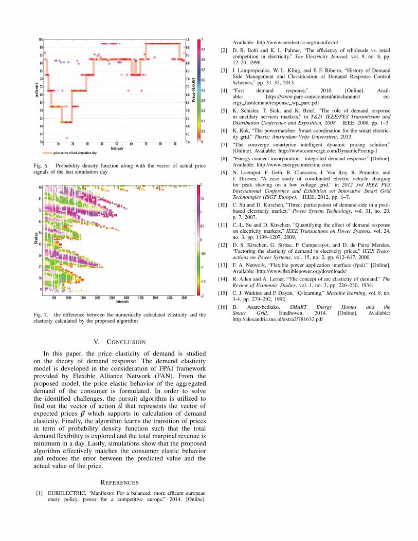
each simulation day (i.e. after every 96 intervals). Since actionsare the representation of prices so the vector of expected prices~p could be easily generated. On the other hand, in the lastinterval of each simulation day; (a) the absolute error betweenthe expected price and real price is calculated as shown in Fig.5 and (b) probability density function is updated by using (12). Fig. 6 shows the p.d.f of the last simulation day and it isobserved that the algorithm has learned the price transitionbecause the line in figure matches the p.d.f., where the lineshows the vector of prices of last simulation day. Moreover,it is also observed from Fig. 5 that the absolute error alsodecreases as the learning proceeds.
Lastly, difference between the numerically calculated elas-ticity and the elasticity calculated by the proposed algorithmis shown in Fig. 7. It is seen that the differences were highduring the initial phase of learning in the same fashion asshown in Fig. 5. Moreover, it is also observed from Fig. 7 thatthe elasticity is usually less predictable for the end of the dayduring every simulation cycle. It is so because the smart homemodel tries to allocate all the non-utilized flexibility in the endof the day which makes the demand inelastic during the endof the day. For the same reason, few spikes can also be seenin Fig. 5 even at the end of the simulation timeframe.
Thus from the results, two major conclusions are made.First by using the proposed approach the DA would learn theconsumer behavior in few days period even if it is not initiallyprovided with any past information. Secondly, the proposedapproach would help the EA to manage the bid in-advancesuch that it effectively cope the situation of being inelasticduring the end of the day.
Intervals
act
ion
s
0 10 20 30 40 50 60 70 80 9038
43
48
53
58
63
68
73
78
83
88
93
98
103
0
0.1
0.2
0.3
0.4
0.5
0.6
0.7
0.8
0.9
1
price vector of last simulation day
Pri
ce (
€/k
W)
3.8
4.3
4.8
5.3
5.8
6.3
6.8
7.3
7.8
8.3
8.8
9.3
9.8
1.0
Fig. 6. Probability density function along with the vector of actual pricesignals of the last simulation day.
Intervals
500 1000 1500 2000 2500 3000 3500 4000 4500 5000
9
18
27
36
45
54
63
72
81
90
−2
−1.5
−1
−0.5
0
0.5
1
1.5
2
Sta
tes
Fig. 7. the difference between the numerically calculated elasticity and theelasticity calculated by the proposed algorithm
V. CONCLUSION
In this paper, the price elasticity of demand is studiedon the theory of demand response. The demand elasticitymodel is developed in the consideration of FPAI frameworkprovided by Flexible Alliance Network (FAN). From theproposed model, the price elastic behavior of the aggregateddemand of the consumer is formulated. In order to solvethe identified challenges, the pursuit algorithm is utilized tofind out the vector of action ~a that represents the vector ofexpected prices ~p which supports in calculation of demandelasticity. Finally, the algorithm learns the transition of pricesin term of probability density function such that the totaldemand flexibility is explored and the total marginal revenue isminimum in a day. Lastly, simulations show that the proposedalgorithm effectively matches the consumer elastic behaviorand reduces the error between the predicted value and theactual value of the price.
REFERENCES
[1] EURELECTRIC, “Manifesto: For a balanced, more efficent europeanenery policy, power for a competitive europe,” 2014. [Online].
Available: http://www.eurelectric.org/manifesto/
[2] D. R. Bohi and K. L. Palmer, “The efficiency of wholesale vs. retailcompetition in electricity,” The Electricity Journal, vol. 9, no. 8, pp.12–20, 1996.
[3] I. Lampropoulos, W. L. Kling, and P. F. Ribeiro, “History of DemandSide Management and Classification of Demand Response ControlSchemes,” pp. 31–35, 2013.
[4] “Fast demand response,” 2010. [Online]. Avail-able: https://www.parc.com/content/attachments/ en-ergy fastdemandresponse wp parc.pdf
[5] K. Schisler, T. Sick, and K. Brief, “The role of demand responsein ancillary services markets,” in T&D. IEEE/PES Transmission and
Distribution Conference and Exposition, 2008. IEEE, 2008, pp. 1–3.
[6] K. Kok, “The powermatcher: Smart coordination for the smart electric-ity grid,” Thesis: Amsterdam Vrije Universiteit, 2013.
[7] “The comverge smartprice intelligent dynamic pricing solution.”[Online]. Available: http://www.comverge.com/DynamicPricing-1
[8] “Energy connect incorporation - integrated demand response.” [Online].Available: http://www.energyconnectinc.com
[9] N. Leemput, F. Geth, B. Claessens, J. Van Roy, R. Ponnette, andJ. Driesen, “A case study of coordinated electric vehicle chargingfor peak shaving on a low voltage grid,” in 2012 3rd IEEE PES
International Conference and Exhibition on Innovative Smart Grid
Technologies (ISGT Europe). IEEE, 2012, pp. 1–7.
[10] C. Su and D. Kirschen, “Direct participation of demand-side in a pool-based electricity market,” Power System Technology, vol. 31, no. 20,p. 7, 2007.
[11] C.-L. Su and D. Kirschen, “Quantifying the effect of demand responseon electricity markets,” IEEE Transactions on Power Systems, vol. 24,no. 3, pp. 1199–1207, 2009.
[12] D. S. Kirschen, G. Strbac, P. Cumperayot, and D. de Paiva Mendes,“Factoring the elasticity of demand in electricity prices,” IEEE Trans-
actions on Power Systems, vol. 15, no. 2, pp. 612–617, 2000.
[13] F. A. Network, “Flexible power application interface (fpai).” [Online].Available: http://www.flexiblepower.org/downloads/
[14] R. Allen and A. Lerner, “The concept of arc elasticity of demand,” The
Review of Economic Studies, vol. 1, no. 3, pp. 226–230, 1934.
[15] C. J. Watkins and P. Dayan, “Q-learning,” Machine learning, vol. 8, no.3-4, pp. 279–292, 1992.
[16] B. Asare-bediako, SMART Energy Homes and the
Smart Grid, Eindhoven, 2014. [Online]. Available:http://alexandria.tue.nl/extra2/781632.pdf