the deviant dynamics of death in heterogeneous populations...
TRANSCRIPT

THE DEVIANT DYNAMICS OF DEATH
IN HETEROGENEOUS POPULATIONS
James W. Vat:pel INTERNATIONAL INSTITUTE
FOR APPLIED SYSTEMS ANALYSIS
AND
DUKE UNIVERSITY
Anatoli I. Yashin INTERNATIONAL INSTITUTE
FOR APPLIED SYSTEMS ANALYSIS
AND
USSR ACADEMY OF SCIENCES
179
JAMES W. VAUPEL AND ANATOLI I. YASHIN
The simplest kind of life-cycle process involves one transition that leads to exit. Examples abound. Animals and plants die, the
healthy fall ill, the unemployed find jobs, the childless reproduce, and the married divorce. Residents move out, machines wear out, natural resources get used up, and buildings are torn down. Infidels convert, ex-convicts recidivate, abstainers become addicted, and holdouts adopt new technologies.
In many such collections or populations, some units are more
likely to make the transition than others. Standard analytic methods
largely ignore this heterogeneity; the methods assume that ail members of a population (or subpopulation, such as black American males) at a
given age face the same probability of change. This chapter presents methods for studying what difference heterogeneity within a popula- tion makes in the behavior of the changing population.
The analytic methods are illustrated by examples drawn from the study of human mortality, and, henceforth, the word death will be used instead of the more general terms change and transition. Readers interested in applications other than human mortality should associate death with an analogous notion like failure, separation, occurrence, or movement.
ROOTS OF THE RESEARCH
A small but growing body of research is relevant to the analysis of differences in behavior over time between heterogeneous and homoge- neous populations. Some strands of this research can be traced to Cournot's study of judicial decisions (1838) and Weinberg's investiga- tion of the frequency of multiple births (1902). Darwin's "population thinking" and emphasis on diversity and selection were crucial contri- butions (Darwin, 1859; Mayr, 1976). Gini (1924) considered hetero-
geneity in female fecundity; Potter and Parker (1964) and Sheps and Menken (1973) developed this approach. In their influential study of the industrial mobility of labor, Blumen, Kogan, and McCarthy (1955) distinguished "movers" from "stayers" and then considered an arbi-
trary number of groups with different proneness to movement; Silcock
The authors thank Brian Arthur, Michael Hannan, Nathan Keyfitz, Howard Kunreuther, Edward Loeser, Mark Pauly, Andrei Rogers, Michael Stoto, and Nancy Tuma for helpful comments.
180
DYNAMICS OF DEATH IN HETEROGENEOUS POPULATIONS
(1954) used a continuous distribution over individuals to describe the "rate of wastage" in labor turnover. This research on the mobility of labor was extended by McFarland (1970), Spilerman (1972), Ginsberg (1973), Singer and Spilerman (1974), and Heckman and Singer (1982); it was generalized to event-history analysis by Tuma (1983) and Tuma and Hannon (1984), among others. Contributions to the analysis of human mortality and morbidity were made by Beard (1963), Shepard and Zeckhauser (1975, 1980), Keyfitz and Littman (1980), and Vaupel, Manton, and Stallard (1979).
This rich body of research indicates that there is a core of mathe- matical methods that can be usefully applied to the analysis of heteroge- neity in such diverse phenomena as accidents, illness, death, fecundity, labor turnover, migration, and equipment failure. These sundry ap- plications and the varied disciplinary backgrounds of the researchers make it hardly surprising that key elements of this common core of mathematics were independently discovered by several researchers. Further progress, however, surely would be accelerated if the wide
applicability of the underlying mathematics of heterogeneity were rec-
ognized.
A UNIFYING QUESTION
Building on this body of research and, most directly, on Vaupel, Manton, and Stallard (1979), this chapter addresses a basic question: How does the observed rate of death, over time, for a cohort of individ- uals born at the same time relate to the probability of death, over time, for each of the individuals of the cohort?1 This question provides a
unifying focus for developing the mathematical theory of the dynamics of heterogeneous populations. It is also a useful question in applied
1 The word rate means different things to different specialists. In this chapter, rate of death is a measure of the likelihood of death at some instant. The phrase rate of death as used here has numerous aliases, including hazard rate and force of mortality. The rate of death for an individual, or individual death rate, is defined by Equation (la); the cohort death rate is defined by Equation (Ib). Note that rate of death, as used here, is neither a probability nor an average over some time period. Furthermore, note that the rate of death for an individual is a function of that individual's probability of death at some instantaneous age conditional on the individual's surviving to that age. Some readers may find it helpful to read "force of mortality" whenever the phrase rate of death appears.
181
JAMES W. VAUPEL AND ANATOLI I. YASHIN
work because researchers usually observe population death rates but often are interested in individual death rites. The effect of a policy or intervention may depend on individual responses and behavior. Fur- thermore, individual rates may follow simpler patterns than the com-
posite population rates. And explanation of past rates and prediction of future rates may be improved by considering changes on the individ- ual level.
It turns out that the deviation of individual death rates from
population rates implies some surprising and intriguing results. Death rates for individuals increase more rapidly than the observed death rate for cohorts. Eliminating a cause of death can decrease subsequent ob- served life expectancy. A population can suffer a higher death rate at older ages than another population even though its members have lower death rates at all ages. A population's death rate can be increas-
ing even though its members' death rates are decreasing. The theory leads to some methods that may be of use to policy
analysts in evaluating the effects of various interventions-for exam-
ple, a medical care program that reduces mortality rates at certain
ages. The theory also yields predictions that may be of considerable interest to policy analysts. In the developed countries of the world, for
example, death rates after age 70 and especially after age 80 may de- cline faster - and at an accelerating rate -than now predicted by var- ious census and actuarial projections. As a result, pressures on social
security and pension systems may be substantially greater than ex-
pected.
MATHEMATICAL PRELIMINARIES
Let Q be some set of parameters wo. Assume that each parame- ter value characterizes a homogeneous class of individuals and that the
population is a mix of these homogeneous classes in proportions given by some probability distribution on Q.
Denote by p,,(a) the probability that an individual from homoge- neous class ow will be alive at age a, and let /,(a) be the instantaneous
age-specific death rate at age a for an individual in class ow. By defini-
tion,
,(a) = - [dpo(a)/da] /p,(a)
182
(la)
DYNAMICS OF DEATH IN HETEROGENEOUS POPULATIONS
Similarly, let p(a) be the probability that an arbitrary individual from the population will be alive at age a. That is, let p(a) be the
expected value of the probability of surviving to age a for a randomly chosen individual at birth. Alternatively, p(a) can be interpreted as the
expected value of the proportion of the birth cohort that will be alive at
age a. The cohort death rate #(a) is then defined by
A(a)= -[dp(a)/da] /p(a) (1 b)
Throughout this chapter, superscript bars will be used to denote vari- ables pertaining to expected values either for a randomly chosen indi- vidual at birth or, equivalently, for the entire cohort.
Suppose that all individuals in a population are identical and their chances of survival are described by p(a). Then p(a) is the same as
p(a). Thus a cohort described by p(a) could be interpreted as being a
homogeneous population composed of identical individuals each of whom had life chances given by p(a) equaling p(a). This remarkable fact means that researchers interested in population rates can simplify their analysis by ignoring heterogeneity; this simplification has permit- ted the development of demography, actuarial statistics, reliability engi- neering, and epidemiology.
For some purposes, however, the simplification is inadequate, counterproductive, or misleading. Sometimes researchers are inter- ested in individual rather than population behavior, sometimes patterns on the individual level are simpler than patterns on the population level, and sometimes the impact of a policy intervention can be correctly predicted only if the varying responses of different individuals are taken into account. That is, sometimes individual differences make enough difference that it pays to pay attention to them; a variety of specific examples are given later in the chapter. Furthermore, the complexi- ties introduced by heterogeneity are not intractable; indeed, the mathe- matical methods presented in this chapter are fairly simple.
BASIC MATHEMATICAL FORMULATION
In mortality analysis, the adjective heterogeneous usually implies that individuals of the same age differ in their chances of death. As in
many other problems involving relative measurement, it is useful to have some standard or baseline to which the death rates of various individuals can be compared. Let u(a) be this baseline death rate; how
183
JAMES W. VAUPEL AND ANATOLI I. YASHIN
values of u(a) might be chosen will be discussed later. The relative risk for individuals in homogeneous class co at time a will be defined as
z(a, co) = ,((a)//(a) (2)
It is convenient to use u(a,z) to denote the death rate at time a of individuals at relative risk z. Clearly
u(a,z) = zu(a) (3)
Thus
l(a) = u(a, 1) (4)
The standard death rate ,u(a) can therefore be interpreted as the death rate for the class of individuals who face a relative risk of 1.
This formulation is simple and broadly applicable. More im-
portant, it yields a powerful result that is central to the mathematics of
heterogeneity. Letfa(z) denote the conditional density of relative risk
among survivors at time a. As shown in Vaupel, Manton, and Stallard
(1979) the expected death rate in the population i(a) is the weighted average of the death rates of the individuals who comprise the popula- tion:
f0 A(a)= f (a,z)fa(z)dz (5)
Since z(a), the mean of the relative-risk values of time a, is given by
z(a)= f zf(z)dz (6) o
it follows from (3) that
A/(z) = /(a)z(a) (7)
This simple result is the fundamental theorem of the mathemat- ics of heterogeneity, since it relates the death rate for the population to the death rates for individuals. The value of/u(a) gives the death rate for the hypothetical "standard" individual facing a relative risk of 1;
multiplying ,(a) by z gives the death rate for an individual facing a relative risk of z. The value of z(a) gives the average relative risk of the
surviving population at time a. In interpreting z(a) it may be useful,
following Vaupel and colleagues, to view z as a measure of "frailty" or
184
DYNAMICS OF DEATH IN HETEROGENEOUS POPULATIONS
"susceptibility." Thus z(a) measures the average frailty of the surviv-
ing cohort.
UNCHANGING FRAILTY
The relationship over time of (a) versus ,u(a) is determined by the trajectory of z(a). The simplest case to study is the case where individuals are born at some level of relative risk (or frailty) and remain at this level all their lives. In this case, the only factor operating to
change z(a) is the higher mortality of individuals at higher levels of relative risk; thus this pure case most clearly reveals the effects of differ- ential selection and the survival of the fittest.
Imagine a population cohort that is born at some point in time.
Letfo(z) describe the proportion of individuals in the population born at various levels of relative risk z;fo(z) can be interpreted as a probability density function. Assume that each individual remains at the same level ofz for life. For convenience, the mean value offo(z) might as well be taken as 1, so that the standard individual at relative risk 1 is also the mean individual at birth and hence,u(O) equals,u(0). As before, let u(a,z) and ,u(a) be the death rates of individuals at relative risk z and of the standard individual. Let H(a,z) be the cumulative hazard experienced from birth to time a:
H(a,z)= j #(a,z)da (8)
Clearly
H(a,z) = zH(a) (9)
The probability that an individual at relative risk z will survive to age a is
given by
p(a,z) = p(a)z = exp[-zH(a)] (10)
Consequently
fa(z) =fo(z) exp[-zH(a)]/ fo(z) exp[-zH(a)]dz (11)
where the denominator is a scaling factor equal to p(a), the proportion
185
JAMES W. VAUPEL AND ANATOLI I. YASHIN
of the population cohort that has survived to age a. Thus
z(a)= f zfo(z) exp[-zH(a)]dz/ ffo(z) exp[-zH(a)]dz (12)
Differentiating Equation (12) with respect to a yields
dz(a)/da = -u(a)2(a) (13)
where a2(a) is the conditional variance of z among the population that is alive at time a. Since fu(a) > 0 and 2(a) > 0, the value ofdz(a)/da must be negative. Therefore, as might be expected, the mean relative risk declines in time as death selectively removes the frailest members of the
population. This means that i(a) increases more rapidly than ju(a). Mean relative risk declines monotonically not only with age (or
time) a but also with the proportion surviving p. This can be shown as follows. If,l(a) is greater than zero for all a, then
z(a) > z(b) if and only if a < b (14)
and
p(a) > p(b) if and only if a < b (15)
Consequently
Z[p-L(P)] < [p-1(p*)] if and only if f < * (16)
where -l(p) is the inverse function of p(a) and where p and p* are two
specific values of the survival function.
HOW j DIVERGES FROM ,u
The magnitude of the divergence I,(a) from u(a) depends on the distribution of relative risk. Several researchers in different fields, including Silcock (1954), Spilerman (1972), Mann, Schafer, and Sing- purwalla (1974), and Vaupel, Manton, and Stallard (1979), have discov- ered that the gamma distribution is especially convenient to work with, since it is one of the best-known nonnegative distributions, it is analytic- ally tractable, and it takes on a variety of shapes depending on parame- ter values. If the mean relative risk at birth is 1, then the gamma probability density function at birth is given by
fo(z) = kkz*-I exp(- kz)/F(k)
186
(17)
DYNAMICS OF DEATH IN HETEROGENEOUS POPULATIONS
where k, the so-called shape parameter, equals (when the mean is 1) the inverse of the variance U2. When k = 1, the distribution is identical to the exponential distribution; when k is large, the distribution assumes a
bell-shaped form reminiscent of a normal distribution. If relative risk at birth is gamma-distributed with mean 1, it can
be shown (see Vaupel, Manton, and Stallard, 1979) that
z(a) = p(a)a2 = exp[- c2 H(a)] = exp - 2 f i(a)da (18)
and that
?(a) = 1/[1 + 2H(a)] (19)
Thus the relationship of At(a) to ii(a), as determined by z(a), can be determined by the cumulative hazard for either the population or the standard individual. In the special case where q2 = 1, the value of z(a) falls off with p(a), the proportion of the cohort that is surviving. It also can be shown (Vaupel, Manton, and Stallard, 1979) thatfa(z) is gamma- distributed with a mean of z(a) and a shape parameter equal to the same value of k at birth.
These results for the gamma distribution with mean 1 at birth are easily generalized to the case of any mean z(0) at birth. Equation (18) then becomes
z(a) = ?(0)p(a)a (20)
and Equation (19) becomes
z(a) = z(0)/[1 + a2 z(O)H(a)] (21)
There is, however, little reason to use this generalized formulation. Let
z*(a) = z(a)/z(O) (22a)
and
A*(a) = A(a)/z(0) (22b)
This simple transformation converts Equations (20) and (21) back to
(18) and (19). Furthermore, as indicated earlier, the standard death rate Ju(a) might as well be associated with the mean individual at birth.
Instead of working with a gamma distribution, it might seem more natural to assume that there is some normally distributed risk
187
JAMES W. VAUPEL AND ANATOLI I. YASHIN
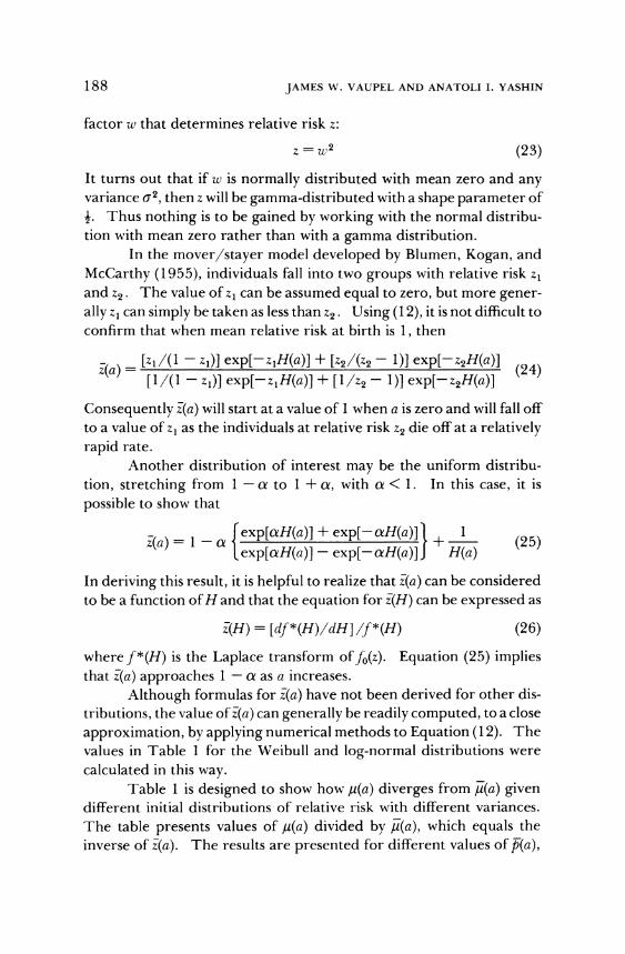
factor w that determines relative risk z:
z =w2 (23)
It turns out that if w is normally distributed with mean zero and any variance a2, then z will be gamma-distributed with a shape parameter of i. Thus nothing is to be gained by working with the normal distribu- tion with mean zero rather than with a gamma distribution.
In the mover/stayer model developed by Blumen, Kogan, and
McCarthy (1955), individuals fall into two groups with relative risk zl and Z2. The value of z1 can be assumed equal to zero, but more gener- ally zl can simply be taken as less than z2. Using (12), it is not difficult to confirm that when mean relative risk at birth is 1, then
(a) = [z/( - z()] exp[-zlH(a)] + [z2/(2 - 1)] exp[-z2H(a)] (24)
[1/(1 - z1)] exp[-z, H(a)] + [1/z2 - 1)] exp[-z2H(a)]
Consequently z(a) will start at a value of 1 when a is zero and will fall off to a value of z1 as the individuals at relative risk z2 die off at a relatively rapid rate.
Another distribution of interest may be the uniform distribu- tion, stretching from 1 - a to 1 + a, with a < 1. In this case, it is
possible to show that
z(a) = 1- r exp[aH(a)] + exp[-H(a)] + 1 (25) (a)
exp[aH(a)] - exp[-aH(a)] J H(a)
In deriving this result, it is helpful to realize that z(a) can be considered to be a function of H and that the equation for z(H) can be expressed as
z(H) = [df *(H)/dH] /f *(H) (26)
wheref*(H) is the Laplace transform off0(z). Equation (25) implies that z(a) approaches 1 - a as a increases.
Although formulas for z(a) have not been derived for other dis- tributions, the value ofz(a) can generally be readily computed, to a close
approximation, by applying numerical methods to Equation (12). The values in Table 1 for the Weibull and log-normal distributions were calculated in this way.
Table 1 is designed to show how t(a) diverges from iu(a) given different initial distributions of relative risk with different variances. The table presents values of u(a) divided by t-(a), which equals the inverse of z(a). The results are presented for different values of p(a),
188

DYNAMICS OF DEATH IN HETEROGENEOUS POPULATIONS
TABLE 1
Divergence of , from i
Variance and Forms of Initial Distribution Values of //l When p Is
of Relative Risk 1.00 0.75 0.50 0.25 0.10 0.05
a2 = 0.1 Gamma 1.00 1.03 1.07 1.15 1.26 1.35 Weibull 1.00 1.03 1.08 1.17 1.34 1.49
Log normal 1.00 1.03 1.07 1.14 1.23 1.30 a2 = 1
Exponentiala 1.00 1.33 2.00 4.00 10.00 20.00
Log normal 1.00 1.27 1.64 2.30 3.33 4.24 2 = 2
Gamma 1.00 1.78 4.00 16.00 100.00 400.00 Weibull 1.00 1.70 3.32 9.56 36.10 99.00
Log normal 1.00 1.49 2.23 3.46 5.61 7.65
a When a2 = 1, the gamma and Weibull distributions are identical to the exponential distribution.
the proportion of the initial population that is surviving; presenting the results for values of p(a) rather than for values of a is convenient since
assumptions about the rate of aging (that is, about how u(a) changes with
a) do not have to be made. Table 1 indicates that u(a) can be substan-
tially greater than /u(a) when only a fraction of the population is alive. Even when the variance in relative risk is only 0.1 (compared with a mean level of birth of 1), u(a) is 30 to 50 percent higher than i(a) when 5
percent of the population is surviving. As the table demonstrates, the
degree of divergence of u(a) from ui(a) depends on both the form of the initial distribution of relative risk and the variance of this distribution.
THE SHAPE OF THE AGING TRAJECTORY
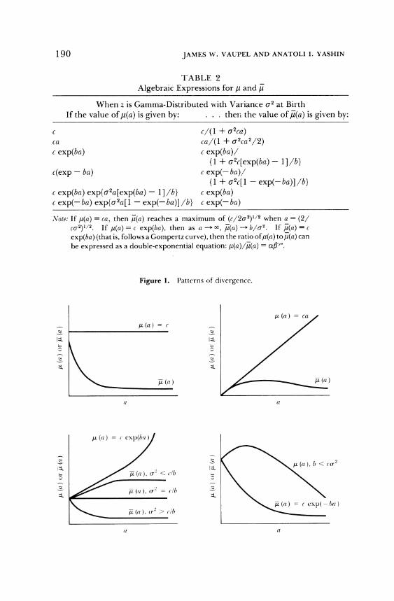
Although Table 1 and Equations (18), (19), (24), and (25) pro- vide information about the divergence between the death rate for the standard individual, ,u(a), and the observed cohort death rate, iu(a), analysis of the shape of,u(a) and iu(a) requires some assumptions about how one of these two curves increases with a. If relative risk at birth is
gamma-distributed with mean 1 and variance a2, the correspondence between six different formulas for Ju(a) and iu(a) is as given in Table 2.
Figure 1 depicts how the curves for j(a) and li(a) diverge in four cases.
189
JAMES W. VAUPEL AND ANATOLI I. YASHIN
TABLE 2
Algebraic Expressions for , and )t
When z is Gamma-Distributed with Variance cr2 at Birth If the value of ,(a) is given by: . . . theni the value of i(a) is given by:
c c/(l + a2ca) ca ca/(1 + a2ca2/2) c exp(ba) c exp(ba)/
(1 + a2c[exp(ba) - l]/b}
c(exp - ba) c exp(-ba)/ (1 + a2c[1 - exp(-ba)]/b}
c exp(ba) exp(a2a[exp(ba) - ] /b} c exp(ba) c exp(-ba) exp(a2a[1 - exp(-ba)]/b} c exp(-ba)
Note: If t(a) = ca, then /(a) reaches a maximum of (c/2a2)1/2 when a = (2/ ca2)1/2. If ,u(a) = c exp(ba), then as a -- o, i(a) -' b/a2. If /(a) = c
exp(ba) (that is, follows a Gompertz curve), then the ratio of,u(a) to /(a) can be expressed as a double-exponential equation: /(a)/a)(a) = a,?Y.
Figure 1. Patterns of divergence.
A (a) = c _
At ((a)
a
190
(I
DYNAMICS OF DEATH IN HETEROGENEOUS POPULATIONS
Table 2 and Figure 1 clearly demonstrate that the pattern of individual
aging can differ radically from the observed pattern of aging in the
surviving cohort. When #(a) is constant, for instance, u(a) declines with
age; heterogeneity introduces spurious age dependence on the popula- tion level (McFarland, 1970; also see Beard, 1963).
THE DISTRIBUTION OF LIFE SPANS
Although the discussion so far has focused on the divergence ofu and ,u over time, comparisons of individual versus cohort behavior in
heterogeneous populations could also be expressed in terms of other statistics. Consider, for example, the fractiles of the distribution of life
spans or, equivalently, the distribution of age of death. Table 3
presents some of these fractiles for a population and for individuals. Fractiles for the standard individual are given for three levels of hetero-
geneity as measured by a2; fractiles are also presented for individuals at three levels of relative risk z. The calculations assume that relative risk is gamma-distributed with mean 1 at birth and that the observed death rate for the population is given by a Gompertz function, c exp(ba), where c equals 0.00012 and b equals 0.085. Table 3 indicates that the distribution of life spans in a population is more spread out than the distribution of possible life spans for an individual. In particular, the
right-hand tail of the distribution is shorter for individuals, especially for robust individuals where variance in heterogeneity is high.
MORTALITY CONVERGENCE AND CROSSOVER
For many pairs of populations, reported mortality rates con-
verge and even cross over with age. In the United States, for example, blacks have lower mortality rates than whites after age 75 or so (Manton and Stallard, 1981). In most developed countries, male and female death rates converge in old age. Nam, Weatherby, and Ockay (1978) present statistics on this and a variety of other convergences and cross- overs.
These reported convergences and crossovers of population death rates may be the result of age misreporting or actual individual differences in rates of aging. To some extent, they may also be artifacts of heterogeneity in individual death rates. Let r(a) denote the ratio of
191
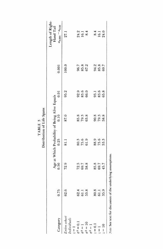
TABLE 3 Distribution of Life Spans
Length of Right- Age at Which Probability of Being Alive Equals Hand Tail
Category 0.75 0.50 0.25 0.10 0.01 0.001 ao.00o -ao.50
Entire cohort 62.6 72.9 81.1 87.0 95.2 100.0 27.1 Individuals z= 1 a2 = 0.1 62.4 72.5 80.3 85.8 92.9 96.7 24.2 a2 = 1 61.1 69.7 75.6 79.3 83.6 85.8 16.1 a2 = 10 53.8 58.8 61.9 63.8 66.0 67.2 8.4 a2 = 1
z= 0.1 80.8 85.8 88.9 90.8 93.1 94.2 8.4 z= 1 61.1 69.7 75.6 79.3 83.6 85.8 16.1 z= 10 35.9 45.7 53.3 58.8 65.8 69.7 24.0
Note: See text for discussion of the underlying assumptions.
DYNAMICS OF DEATH IN HETEROGENEOUS POPULATIONS
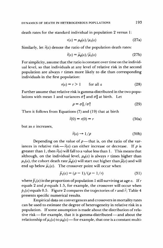
death rates for the standard individual in population 2 versus 1:
r(a) = #U2(a)/1ul(a) (27a)
Similarly, let r(a) denote the ratio of the population death rates:
r(a) = ,2(a)/ul(a) (27b)
For simplicity, assume that the ratio is constant over time on the individ- ual level, so that individuals at any level of relative risk in the second
population are always r times more likely to die than corresponding individuals in the first population:
r(a) = r > 1 for all a (28)
Further assume that relative risk is gamma-distributed in the two popu- lations with mean 1 and variances a and a at birth. Let
p= a/a2 (29)
Then it follows from Equations (7) and (19) that at birth
r(O)= r(O) = r (30a)
but as a increases,
r(a) Il/p (30b)
Depending on the value of p-that is, on the ratio of the var- iances in relative risk-r(a) can either increase or decrease. If p is
greater than 1, then r(a) will fall to a value less than 1. This means that
although, on the individual level, jt2(a) is always r times higher than
#l(a), the cohort death rate (u2(a) will start out higher than /(a) and will end up below Jl(a). The crossover point will occur when
p,(a) = (p- 1)/(p- 1/r) (31)
where p (a) is the proportion of population 1 still surviving at age a. Ifr
equals 2 and p equals 1.5, for example, the crossover will occur when
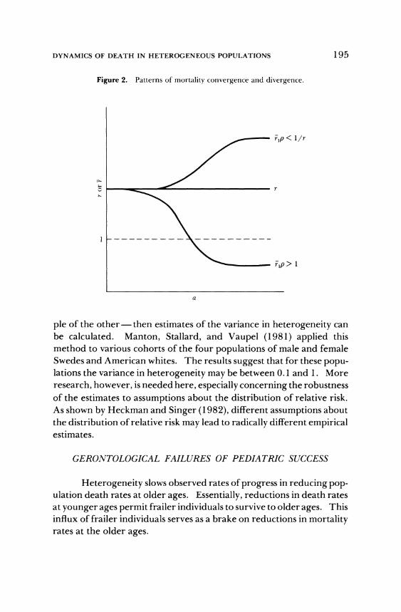
pl(a) equals 0.5. Figure 2 compares the trajectories of r and r; Table 4
presents specific numerical results.
Empirical data on convergences and crossovers in mortality rates can be used to estimate the degree of heterogeneity in relative risk in a
population. If some assumption is made about the distribution of rela- tive risk - for example, that it is gamma-distributed -and about the
relationship oful(a) to /u2(a) - for example, that one is a constant multi-
193
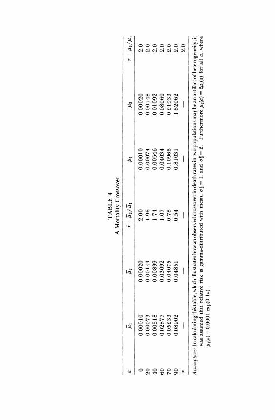
TABLE 4 A Mortality Crossover
a J1 /,2 r= -2/I PI1 I2 r = U2/,
0 0.00010 0.00020 2.00 0.00010 0.00020 2.0 20 0.00073 0.00144 1.96 0.00074 0.00148 2.0 40 0.00518 0.00899 1.74 0.00546 0.01092 2.0 60 0.02877 0.03092 1.07 0.04034 0.08069 2.0 70 0.05233 0.04075 0.78 0.10966 0.21933 2.0 90 0.08902 0.04851 0.54 0.81031 1.62062 2.0
o- -- - 2.0
Assumptions: In calculating this table, which illustrates how an observed crossover in death rates in two populations may be an artifact of heterogeneity, it was assumed that relative risk is gamma-distributed with mean, aI = 1, and ar = 2. Furthermore u2(a) = 2jul(a) for all a, where
=l(a)= 0.0001 exp(0.la).
DYNAMICS OF DEATH IN HETEROGENEOUS POPULATIONS
Figure 2. Patterns of mortality convergence and divergence.
rlp < /r
rlp > 1
pie of the other -then estimates of the variance in heterogeneity can be calculated. Manton, Stallard, and Vaupel (1981) applied this method to various cohorts of the four populations of male and female Swedes and American whites. The results suggest that for these popu- lations the variance in heterogeneity may be between 0.1 and 1. More research, however, is needed here, especially concerning the robustness of the estimates to assumptions about the distribution of relative risk. As shown by Heckman and Singer (1982), different assumptions about the distribution of relative risk may lead to radically different empirical estimates.
GERONTOLOGICAL FAILURES OF PEDIATRIC SUCCESS
Heterogeneity slows observed rates of progress in reducing pop- ulation death rates at older ages. Essentially, reductions in death rates at younger ages permit frailer individuals to survive to older ages. This influx of frailer individuals serves as a brake on reductions in mortality rates at the older ages.
195
1
JAMES W. VAUPEL AND ANATOLI I. YASHIN
As a simple illustration, divide life into two parts - youth and old
age, say--at age a0. Suppose that a proportion p(ao) of every birth cohort used to survive to age a0, but that because of some pediatric advance a proportion p*(ao), greater than p(ao), now survives. Because z increases with p monotonically, z(ao) will increase. Consequently, if the values u(a), where a is greater than a0, remain the same, the values of
,u(a), where a is greater than ao, will increase. If observed death rates at
younger ages are reduced to low levels, however, further progress will add fewer and fewer additional persons to the ranks of the elderly. Thus progress in reducing population mortality rates will not be slowed to the extent it previously was.
Until now this chapter has focused on a single cohort aging through time; thus a represents both age and time. Generalization to the case of multiple cohorts is straightforward: Let #u(a,t), ji(a,t), and
z(a,t) be the values of/ , /i, and zfor a cohort of age a in year t. Then the fundamental theorem (7) can be rewritten as
I-(a,t) = u(a,t)z(a,t) (32)
and it follows that
O#-(a,t)/8t a (a,t)/Ot + 9z(a,t)/dt + (33) u(a, t) y(a, t) z(a,t)
Let
7a(t) a(a,t)t (34a) #(a,t)
and
Z7a(t) =- O )/ (34b) U(a,t)
Thus 7r and d are measures of the rate of progress in reducing individual and population death rates. Equation (33) can be rewritten as
7-a(t) = 7a(t)- (a,t)(35)
When individuals remain at the same level of relative risk for life,
progress in reducing individual death rates will reduce the value of the
negative term in this formula; at any age a the value of z(a,t) will ap- proach 1 as t increases, and the value of d(z)(a,t)/dt will approach zero.
196

DYNAMICS OF DEATH IN HETEROGENEOUS POPULATIONS
This is easy to see in the special case where relative risk is gamma-distrib- uted at birth with a mean and variance of 1. Then z(a) equals p(a) so that
Oz(a,t)/dy _ dp(a,t)/t (36)
z(a,t) p(a,t)
The proportion surviving at any age a will clearly approach 1 as prog- ress in reducing death rates continues. Furthermore, the change over time in the proportion surviving will approach zero.
Equation (35) consequently indicates that as progress in reducing individual death rates continues,
7za(t) -
a(t) for any a (37)
Since progress in reducing death rates permits frailer individuals to survive to older ages,
8z(a,t)/da < 0 (38)
But, of course, z(a,t) is greater than zero. Therefore
7a(t) < 7Ta(t) for any a (39)
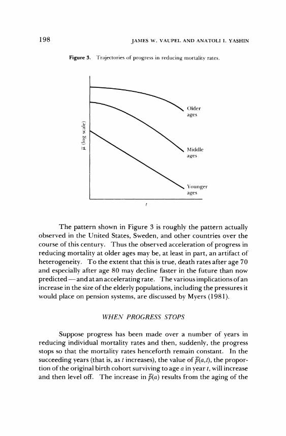
In short, the observed rate of progress in reducing the popula- tion death rate at any age a will be less than, but will eventually ap- proach, the rate of progress in reducing individual death rates at age a. Table 5 presents numerical results concerning 7ta(t) when 7la(t) is con- stant for all a and t; Figure 3 depicts the pattern of these results.
TABLE 5 Acceleration in Observed Rates of Progress in Reducing Mortality Rates
Observed Rate of Progress T(a,t) When Age a Equals Year t 20 40 60 80
0 0.00986 0.00894 0.00528 0.00131 40 0.00991 0.00927 0.00626 0.00184 80 0.00994 0.00950 0.00714 0.00252
120 0.00996 0.00966 0.00788 0.00334 o0 0.01000 0.01000 0.01000 0.01000
Note: It is assumed that the rate of progress on the individual level is 0.01:
[aLu(a,t)/9t]/#(a,t)= = r =0.01 for all a, t
Furthermore, z is assumed to be gamma-distributed with mean 1 and variance 1 at birth and ((a, 0) = 0.0002 exp(0. la).
197
JAMES W. VAUPEL AND ANATOLI I. YASHIN
Figure 3. Trajectories of progress in reducing mortality rates.
Older ages
^I=~~~t \^~ \ Middle ages
X Younger ages
The pattern shown in Figure 3 is roughly the pattern actually observed in the United States, Sweden, and other countries over the course of this century. Thus the observed acceleration of progress in
reducing mortality at older ages may be, at least in part, an artifact of
heterogeneity. To the extent that this is true, death rates after age 70 and especially after age 80 may decline faster in the future than now
predicted - and at an accelerating rate. The various implications of an increase in the size of the elderly populations, including the pressures it would place on pension systems, are discussed by Myers (1981).
WHEN PROGRESS STOPS
Suppose progress has been made over a number of years in
reducing individual mortality rates and then, suddenly, the progress stops so that the mortality rates henceforth remain constant. In the
succeeding years (that is, as t increases), the value of p(a,t), the propor- tion of the original birth cohort surviving to age a in year t, will increase and then level off. The increase in p(a) results from the aging of the
198

DYNAMICS OF DEATH IN HETEROGENEOUS POPULATIONS
younger cohorts that have experienced lower death rates because of the
previous progress. Since, as noted earlier, zis a monotonically increas-
ing function of p, it follows that z will increase as well. The value of
/u(a,t), any a and t, will be constant--that is what no progress means. But then it follows from Equation (32) that ju(a,t) at any age a will increase in time.
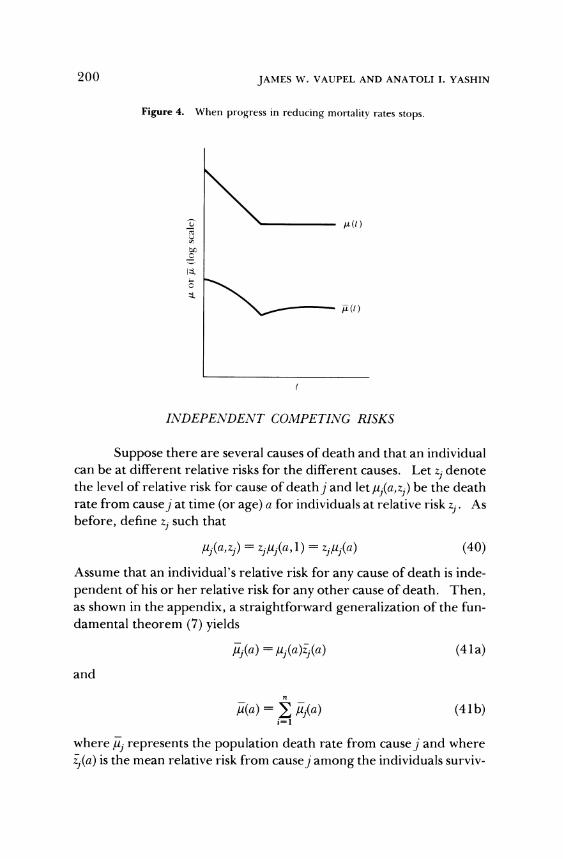
In short, current mortality rates for populations are lower than the mortality rates that would prevail if current mortality rates for individuals persisted. If progress in health conditions stops, death rates will rise. This implies that estimates of current life expectancy are too
high. These estimates are based on current population death rates, but
they are supposed to represent what life expectancy would be if health conditions remained unchanged. Vaupel, Manton, and Stallard (1979) indicate how the correct value of current life expectancy, adjusted for the effects of heterogeneity and past health progress, might be calcu- lated. Table 6 and Figure 4 compare the patterns of #(a,t) and u(a,t) when health progress stops.
If progress in reducing # accelerates and decelerates with time, the observed trajectory of u will be bumpy and might show periods of
apparent negative progress; this phenomenon might underlie the in- crease in death rates observed in the United States in the middle and late 1960s, following a relatively rapid decrease in the 1950s.
TABLE 6 When Progress in Reducing Mortality Rates
Stops
Year t ,u(60,t) li(60,t)
0 0.08069 0.04264 20 0.06606 0.03817 40 0.05409 0.03384 60 0.04428 0.02972 80 0.03625 0.02588 81 0.03625 0.02595 90 0.03625 0.02635 oo 0.03625 0.02662
Assumptions: y(a,O) = 0.0002 exp(0.la) yi(a,t) = #(a,0) exp(-0.0 lt), t < 80 y(a,t) =/ (a,80), t > 80
199
JAMES W. VAUPEL AND ANATOLI I. YASHIN
Figure 4. When progress in reducing mortality rates stops.
, \(t)
br)
(t)
INDEPENDENT COMPETING RISKS
Suppose there are several causes of death and that an individual can be at different relative risks for the different causes. Let zj denote the level of relative risk for cause of deathj and let /u(a,zj) be the death rate from causej at time (or age) a for individuals at relative risk z . As before, define Zj such that
,uj(a,zj) = zj uj(a,l) = zjluj(a) (40)
Assume that an individual's relative risk for any cause of death is inde-
pendent of his or her relative risk for any other cause of death. Then, as shown in the appendix, a straightforward generalization of the fun- damental theorem (7) yields
yj(a) = yj(a)zj(a) (4 la)
and
A(a) = /uj(a) (41b) i=l
where ij represents the population death rate from cause j and where
zj(a) is the mean relative risk from causej among the individuals surviv-
200

DYNAMICS OF DEATH IN HETEROGENEOUS POPULATIONS
ing to time a. The value of zj(a) for any cause of death j can be calcu- lated on the basis offo(zj), the distribution of zj at birth, and iu(a), the death rate from cause j:
zo(zj(P) e p zj1j(s)ds]dzj
fo(zj) exp - zjIj(s)dsdz (42)
Thus the dynamics of mortality from any specific cause of death can be studied without knowing the death rates and distributions of relative risks for other causes of death.
Suppose that the zj are gamma-distributed with mean 1 and var- iances a2. (As before, the means might as well be set equal to 1, as in that case the standard individual at relative risk 1 will be the mean individual at birth.) Then Equation (19) generalizes to
zj(a) = 1/[1 + a2Hj(a)] (43)
where
fa Hj(a)= f j(s)ds (44)
Furthermore, Equation (18) generalizes to
za. p(a) 2(a) (45) Zj( jW .(45)
where pj(a) is the proportion that would survive to age a ifj were the
only cause of death:
pj(a)=exp[- fi(s)ds] (46)
The formulas for the uniform distribution (25) and the two-point distri- bution (24) similarly generalize.
Thus the case of independent, competing risks is almost as easy to analyze as the simpler case of a single cause of death. In a sense the competing risk case adds another dimension of heterogeneity, as now individuals not only differ from each other but also differ within them- selves in susceptibility to various causes of death.
Patterns of aging for individuals can be compared with observed patterns of aging for the surviving cohort in much the same way when
201

JAMES W. VAUPEL AND ANATOLI I. YASHIN
there are several causes of death as when there is only a single cause of death. Figure 5 presents an example. The mortality curve shown in
Figure 5, which is plotted on a log scale, is intriguing because it resem- bles the observed mortality curves of most developed countries: Mortal-
ity falls off after infancy, begins increasing again after age 7 or so, rises
through a hump roughly between ages 15 and 30, and then at older ages increases more or less exponentially. Figure 5 was created by assuming there were three causes of death. For individuals, the incidence of the first cause is constant, the incidence of the second cause increases ex-
ponentially, and the incidence of the third cause increases according to the double-exponential form that produces, on the population level, an observed exponential increase. The three independent causes of death act, on the individual level, as follows: ,i1(a) = 0.02 and zl is gamma-dis-
Figure 5. A population mortality curve produced by three causes of death.
-1.5-
-2.5-
-3.5-
_ /
-4.5-
-5.5-
-6.5-
-7. , v}.......
( 10 20 30 40 50 60 70 80 90
Age
202
DYNAMICS OF DEATH IN HETEROGENEOUS POPULATIONS
tributed with ac = 500; #2(a) = 0.00001 exp(0.04a) and z2 is gamma- distributed with a = 200; #3(a) = a exp(ba) exp(a[exp(ba)
- 1]/ba2),
a = 0.00015, b = 0.08, and Z3 is gamma-distributed with a2 = 1.
Just as mortality convergences and crossovers for two popula- tions may be artifacts of heterogeneity, convergences and crossovers for two causes of death may also be artifacts of heterogeneity. In the earlier discussion of population crossovers, the subscriptj denoted pop- ulation 1 or 2- for example, ij was the death rate for population j. The mathematics is equally valid if the subscriptj denotes cause of death 1 or 2. So, for example, cause of death 2 might be twice as likely as cause of death 1, at all ages, for all individuals. If the variance in z2, however, is greater than twice the variance in zl, the observed rate of death from cause 2 in the surviving cohort will approach and eventually fall below the observed rate for cause 1.
How will progress in reducing individual death rates affect ob- served progress in reducing deaths in surviving cohorts? For any spe- cific cause of death, the mathematics is the same as outlined in the
preceding section on progress. Furthermore, in the case being consid- ered here of independent causes of death, progress in reducing one cause of death will have no effect on uj(a) or iuj(a) for any other cause of
deathj. Since everyone has to die of something, the number of people eventually dying from other causes will increase, but the death rates j and juj will not change.
CORRELATED CAUSES OF DEATH
When causes of death are not independent but are correlated with each other, the mathematics becomes more complicated. The fundamental equations (41 a) and (41 b) are still valid, but now the value of z(a) depends on the death rates and distributions of relative risks for correlated causes of death:
A *
zfo(zl ... Zn) exp[-zl H(a) * - znHn(a)]dzl ... dz
Jo(a)~~~ = Jo~ fcc fcc ~(47) zj(a)= r 0 rJ
a = ...
fo(zl ...zn) exp[-z,Hl(a) *" znH,(a)]dzl ...dzn o fo
203
JAMES W. VAUPEL AND ANATOLI I. YASHIN
where, as before,
fa Hj(a)= /j(s)ds
As a simple example, consider the following special case. Sup- pose that there are two causes of death and that, as in the mover/stayer model, there are two kinds of people. Let ul(a) and /2(a) be the death rates from cause 1 and 2 for the standard individual in the first group, and let u* (a) and #p4(a) be the rates for the second group. Finally, suppose the rates are interrelated as follows:
0 <u *(a) < #l(a) for all a (48a)
and
2*(a) = 0 for all a (48b)
Thus the second, "robust," group does not die from cause 2 and faces a lower death rate than the first group does from cause 1.
Let 7r(a) denote the proportion of the total population that is in the first group at time a. The observed death rate for the first cause of death will be
yl(a) = n(a)#lu(a) + [1 - n(a)], *(a) (49a)
and the observed death rate for the second cause of death will simply be
82(a) = z7(a)/2(a) (49b)
Suppose some progress is made in reducing the incidence of the second cause of death. Then the observed death rate from the first cause will increase. This observed death rate is the weighted average of the death rates for the first and second groups. If death rates for the first group are reduced (as a result of progress against the second cause of death), more of this group will survive. The value of n(a) will in- crease and since #l(a) exceeds jU*(a), the value of ,l(a) will also in- crease. The value of 7(a), by the way, is given by
7(0O) expf- [(s) + ( s)+ ?2()]dsI
(a)= r 1 (50) 7r(0) exp- I [l(s) + 2(s)]ds} + [1 - n(0)] exp[- p (s)ds
204
DYNAMICS OF DEATH IN HETEROGENEOUS POPULATIONS
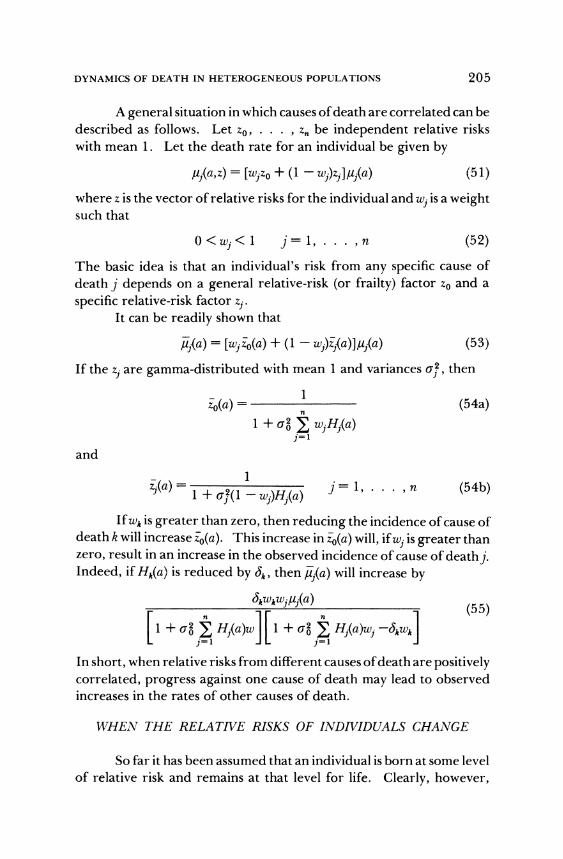
A general situation in which causes of death are correlated can be described as follows. Let z0, . ... , zbe independent relative risks with mean 1. Let the death rate for an individual be given by
ij(a,z) = [wjzo + (1 - wj)zj]#j(a) (51)
where z is the vector of relative risks for the individual and wj is a weight such that
0 < wj j=1, .. ,n (52)
The basic idea is that an individual's risk from any specific cause of death j depends on a general relative-risk (or frailty) factor z0 and a
specific relative-risk factor zj. It can be readily shown that
,(a) = [wjzo(a) + (1 - wj)j(a)]uj(a) (53)
If the zj are gamma-distributed with mean 1 and variances aj, then
z-(a)= (54a) 1 + c'2 wHtj(a)
j=1
and
-(+a)l j(=1-,....Hn (54b)
If wk is greater than zero, then reducing the incidence of cause of death k will increase z0(a). This increase in o0(a) will, if wj is greater than zero, result in an increase in the observed incidence of cause of deathj. Indeed, if Hk(a) is reduced by Jk, then /j(a) will increase by
s5kwkwJ,j(a) (5
[1 -+ o 2 Hj(a)w [1 + a o Hj(a)wj -6a ] j=1 j=1
In short, when relative risks from different causes of death are positively correlated, progress against one cause of death may lead to observed increases in the rates of other causes of death.
WHEN THE RELATIVE RISKS OF INDIVIDUALS CHANGE
So far it has been assumed that an individual is born at some level of relative risk and remains at that level for life. Clearly, however,
205
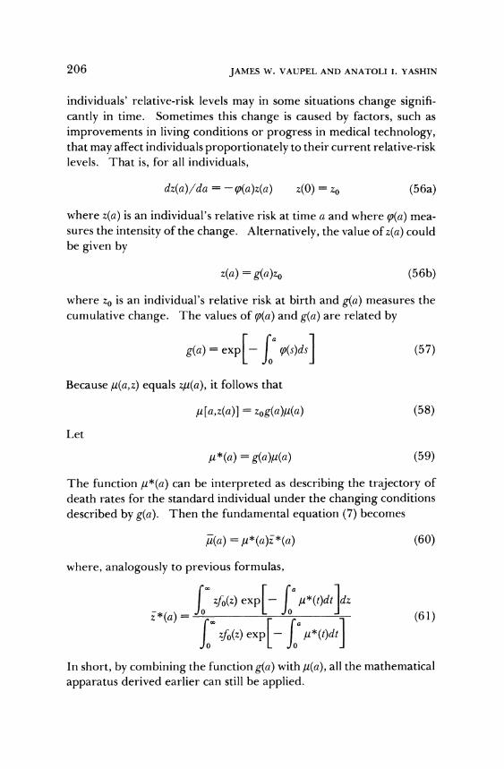
JAMES W. VAUPEL AND ANATOLI I. YASHIN
individuals' relative-risk levels may in some situations change signifi- cantly in time. Sometimes this change is caused by factors, such as
improvements in living conditions or progress in medical technology, that may affect individuals proportionately to their current relative-risk levels. That is, for all individuals,
dz(a)/da = - ((a)z(a) z(0) = Z - (56a)
where z(a) is an individual's relative risk at time a and where (p(a) mea- sures the intensity of the change. Alternatively, the value ofz(a) could be given by
z(a) = g(a)zo (56b)
where z0 is an individual's relative risk at birth and g(a) measures the cumulative change. The values of p(a) and g(a) are related by
g(a) = exp[- f(s)ds] (57)
Because y(a,z) equals z,u(a), it follows that
u[a,z(a)] = zog(a)u(a) (58)
Let
*(a) = g(a) (59)
The function u*(a) can be interpreted as describing the trajectory of death rates for the standard individual under the changing conditions described by g(a). Then the fundamental equation (7) becomes
A(a) = /*(a)z*(a) (60)
where, analogously to previous formulas,
zo(z) exp - *(t)dt dz
z*(a) L J (61) z eo(z)xexp *(t)dtl
In short, by combining the function g(a) with u(a), all the mathematical
apparatus derived earlier can still be applied.
206

DYNAMICS OF DEATH IN HETEROGENEOUS POPULATIONS
CONCLUSION
Individuals, whether people, plants, animals, or machines, differ from one another. Sometimes the differences affect the probability of some major transition, such as dying, moving, marrying, or convert-
ing. In this case the observed dynamics of the behavior of the surviving population - the population that has not yet made the transition - will
systematically deviate from the dynamics of the behavior of any individ- ual in the population. Most of the examples and terminology of this
chapter were drawn from the study of human mortality, but the mathe- matics can be applied to various heterogeneous populations for such
purposes as explaining population patterns, making inferences about individual behavior, and predicting or evaluating the impact of alterna- tive control mechanisms, policies, and interventions.
Among the interesting results discussed in this chapter are:
* Death rates for individuals increase more rapidly than the observed death rates for cohorts.
* Observed mortality convergences and crossovers, both between pop- ulations and between causes of death, may be artifacts of heterogene- ity.
* Progress in reducing mortality at younger ages or from some causes of death may increase observed mortality at older ages or from other causes of death.
* Slow but accelerating rates of mortality progress in old age may be an artifact of heterogeneity with a significant consequence: The elderly population may be substantially larger in the future than currently predicted.
APPENDIX: THE COMPETING RISK CASE
Let frailty be the vector z = (z1, z2 . . z,). Denote by Tj the random death times caused by frailty zj, wherej = 1,2, ... , n, and let T = min T, i = 1, 2, ..., n. Let the density function of T when
frailty z is given be
p(t\z) = zii(t) exp [- zi (a)da] pl i-i J L<iJ
207

JAMES W. VAUPEL AND ANATOLI I. YASHIN
Note that from this formula it follows that
P(T > az) = exp - zi f i(t)dt]
As in the scalar case note that
dP(T - a)/da a= P(T > a)
Denoting by f(a) the density probability function of vector z = (Z1, . z.. , , we have
[dP(T < xlz)/da]f(z)dz A (a)= P(T> a)
or using the formula for (ptz), rr n Ca
-- f E [ zi/i(a) exp[- - zi f i(t)dt f(z)dz Ai(a)=o i p L l o
P(T > a)
Noting that
n Ca
exp Z i i(t)dt f (z)
P(T > a) (
where fa(z) is the conditional probability density function of vector
frailty z = (zl, ... , zn) when the event (T > x) is given, we get the
following for Iu(a):
A(a) = ;ui(a)ii(a) where
(a) = E(zjlT > a)
It is essential to know when zj(a) coincides with zj(a), where
j = E{zjlTj > a) is the conditional frailty that was defined before. For this purpose note that the random event (T > a) may be represented as
{T > a)= n{T > a) i=l
208
DYNAMICS OF DEATH IN HETEROGENEOUS POPULATIONS
The equality z(a) = j(a) means that
E(zl n (Ti > a}) = E(zi,Ti > a)
The last equality may take place only in the case when frailty zj for anyj does not depend on Tk, where j
= k andj, k = 1, 2, . . . , n.
REFERENCES
BEARD, R. E.
1963 "A theory of mortality based on actuarial, biological and medical considerations." In Proceedings of International Population Confer- ence. Vol. 1. New York: International Union for the Scientific
Study of Population. BLUMEN, I., KOGAN, M., AND MCCARTHY, P. J.
1955 The Industrial Mobility of Labor as a Probability Process. Ithaca: Cor- nell University Press.
COURNOT, A. A.
1838 "Memoire sur les applications du calcul des chances a la statistique judiciare" [The application of the calculus of probability tojudicial statistics]. Journal de mathematiques pures et appliquees 3:257-334.
DARWIN, C.
1964 On the Origin of Species. Cambridge, Mass.: Harvard University Press. (Originally published 1859.)
GINI, C.
1924 "Premieres recherches sur la fecondabilite de la femme" [New research on the fecundity of women]. Proceedings of the Interna- tional Mathematics Congress 2:889-892.
GINSBERG, R. B.
1973 "Stochastic models of residential and geographic mobility for het-
erogeneous populations." Environment and Planning 5:113-124. HECKMAN, J. J., AND SINGER, B.
1982 "Population heterogeneity in demographic models." In K. Land and A. Rogers (Eds.), Multidimensional Mathematical Demography. New York: Academic Press.
KEYFITZ, N., AND LITTMAN, G.
1980 "Mortality in a heterogeneous population." Population Studies 33:333-343.
LIPTZER, R. S., AND SHIRYAEV, A. N.
1977 Statistics of Random Processes. New York: Springer-Verlag. MCFARLAND, D. D.
1970 "Intergenerational social mobility as a Markov process: Including a time-stationary Markovian model that explains observed declines in mobility rates." American Sociological Review 35:463-475.
209
JAMES W. VAUPEL AND ANATOLI I. YASHIN
MANN, N. R., SCHAFER, R. E., AND SINGPURWALLA, N. D.
1974 Methodsfor Statistical Analysis of Reliability and Life Data. New York:
Wiley. MANTON, K., AND STALLARD, E.
1981 "Methods for evaluating the heterogeneity of aging processes in human populations using vital statistics data: Explaining the black/ white mortality crossover by a model of mortality selection." Human Biology 53:47-67.
MANTON, K., STALLARD, E., AND VAUPEL, J. W.
1981 "Methods for comparing the mortality experience of heteroge- neous populations." Demography 18:389-410.
MAYR, E.
1976 Evolution and the Diversity of Life. Cambridge, Mass.: Harvard Uni-
versity Press. MYERS, R.
1981 Social Security. Homewood, Ill.: Irwin. NAM, C. B., WEATHERBY, N. L., AND OCKAY, K. A.
1978 "Causes of death which contribute to the mortality crossover ef- fect." Social Biology 25:306-314.
POTTER, R. G., AND PARKER, M. P.
1964 "Predicting the time required to conceive." Population Studies 18:99-116.
SHEPARD, D. S., AND ZECKHAUSER, R. J. 1975 "The assessment of programs to prolong life, recognizing their
interaction with risk factors." Discussion Paper 32D. Cam-
bridge, Mass.: Kennedy School of Government, Harvard Univer-
sity. 1980 "Long-term effects of interventions to improve survival in mixed
populations." Journal of Chronic Diseases 33:413-433. SHEPS, M. C., AND MENKEN, J. A.
1973 Mathematical Models of Conception and Birth. Chicago: University of
Chicago Press. SILCOCK, H.
1954 "The phenomenon of labor turnover."Journal of the Royal Statistical
Society 117:429-440. SINGER, B., AND SPILERMAN, S.
1974 "Social mobility models for heterogeneous populations." In H. L. Costner (Ed.), Sociological Methodology 1973- 1974. San Francisco:
Jossey-Bass. SPILERMAN, S.
1972 "Extensions of the mover-stayer model." AmericanJournal of Sociol-
ogy 78:599-626. TUMA, N. B.
1983 "Effects of labor market structure onjob-shift patterns." Working paper 83-11. Laxenburg, Austria: International Institute for
Applied Systems Analysis.
210
DYNAMICS OF DEATH IN HETEROGENEOUS POPULATIONS 211
TUMA, N. B., AND HANNAN, M. T.
1984 Social Dynamics: Models and Methods. San Diego, Calif.: Academic Press.
VAUPEL,J. W., MANTON, K., AND STALLARD, E.
1979 "The impact of heterogeneity in individual frailty on the dynamics of mortality." Demography 16:439-454.
WEINBERG, W.
1902 "Beitrage zur Physiologie und Pathologie der Mehrlingsgeburten beim Menschen" [The physiology and pathology of multiple human births]. Pfluger's Archiv fir die gesamte Physiologie des Mens- chen und der Tiere 88:346-430.