Draft version January 9, 2019Typeset using LATEX twocolumn style in AASTeX62

The dimming of RW Auriga. Is dust accretion preceding an outburst?

Matıas Garate,1 Til Birnstiel,1 Sebastian Markus Stammler,1 and Hans Moritz Gunther2

1University Observatory, Faculty of Physics, Ludwig-Maximilians-Universitat Munchen, Scheinerstr. 1, 81679 Munich, Germany2MIT, Kavli Institute for Astrophysics and Space Research, 77 Massachusetts Avenue, Cambridge, MA 02139, USA

(Received 2018 October 12; Revised 2018 November 23; Accepted 2018 November 24)

Submitted to ApJ

ABSTRACT

RW Aur A has experienced various dimming events in the last years, decreasing its brightness by

∼ 2 mag for periods of months to years. Multiple observations indicate that a high concentration of

dust grains, from the protoplanetary disk’s inner regions, is blocking the starlight during these events.

We propose a new mechanism that can send large amounts of dust close to the star on short timescales,

through the reactivation of a dead zone in the protoplanetary disk. Using numerical simulations we

model the accretion of gas and dust, along with the growth and fragmentation of particles in this

scenario. We find that after the reactivation of the dead zone, the accumulated dust is rapidly accreted

towards the star in around 15 years, at rates of Md = 6× 10−6 M/yr and reaching dust-to-gas ratios

of ε ≈ 5, preceding an increase in the gas accretion by a few years. This sudden rise of dust accretion

can provide the material required for the dimmings, although the question of how to put the dust into

the line of sight remains open to speculation.

Keywords: accretion, accretion disks — hydrodynamics — protoplanetary disks — stars: individual:

RW Aur A

1. INTRODUCTION

RW Aur A is a young star that in the last decade pre-

sented unusual variations in its luminosity. The star has

about a solar mass, it is part of a binary system, and

is surrounded by a protoplanetary disk showing signa-

tures of tidal interaction (Cabrit et al. 2006; Rodriguez

et al. 2018). The star had an almost constant luminos-

ity for around a century, interrupted only by a few short

and isolated dimmings (see Berdnikov et al. (2017) for

a historical summary) until 2010, when its brightness

suddenly dropped by 2 mag in the V band for 6 months

(Rodriguez et al. 2013). Since 2010, a total of five dim-

ming events have been recorded (see Rodriguez et al.

2013, 2016; Petrov et al. 2015; Lamzin et al. 2017; Berd-

nikov et al. 2017, among others). The dimmings can last

from a few months to two years, and reduce the bright-

ness of the star up to 3 mag in the visual. Moreover,

there is no obvious periodicity in their occurrence, and

Corresponding author: Matıas Garate

mgarate@usm.lmu.de

their origin is not yet clear (a summary of the events

can be found in Rodriguez et al. 2018).

1.1. Observations of RW Aur Dimmings

Some observations in the recent years have shed light

on the nature of RW Aur A dimmings:

During the event in 2014-2015 (Petrov et al. 2015), ob-

servations by Shenavrin et al. (2015) show a increase in

IR luminosity at bands L and M. The authors infer that

hot dust from the inner regions is emitting the infrared

excess, while occluding the starlight and causing the

dimming in the other bands.

Observations by Antipin et al. (2015); Schneider et al.

(2015) found that the absorption from optical to NIR

wavelengths is gray, which could indicate the presence

of large particles causing the dimming (& 1µm), and

measured a dust column density of 2× 10−4 g/cm2,

although a similar absorption may be produced if an

optically thick disk of gas and small grains partially

covers the star (Schneider et al. 2018).

Then, the study of RW Aur A spectra by Facchini et al.

(2016) also found that the inner accretion regions of the

disk are being occluded, and therefore the dimmings

arX

iv:1

810.

0619

4v2

[as

tro-

ph.E

P] 8

Jan

201

9

2 Garate et al.

should come from perturbations at small radii.

Finally, during the dimming in 2016, X-Ray observa-

tions from Gunther et al. (2018) indicate super-Solar

Fe abundances, along with a higher column density of

gas in the line of sight. The high NH/AV found by the

authors is interpreted as gas rich concentrations in the

occluding material, or as a sign of dust growth. Also,

gray absorption was found again during this event.

Given this information, several authors have discussed

what mechanism would put the dust from the innermost

regions of the protoplanetary disk, into the line of sight.

Among the possible explanations are: a warped inner

disk (Facchini et al. 2016; Bozhinova et al. 2016), stellar

winds carrying the dust (Petrov et al. 2015; Shenavrin

et al. 2015), planetesimal collision (Gunther et al. 2018),

and a puffed up inner disk rim (Facchini et al. 2016;

Gunther et al. 2018).

Most of the proposed mechanisms rely on having enough

dust close to the star to cause the dimmings. So the

focus of this paper is to propose a mechanism that can

deliver large amounts of dust to the inner regions of the

protoplanetary disk, by raising the dust accretion rate

through the release of a dust trap.

An increased dust concentration can explain some

aspects of the dimmings, such as the high metallic-

ity (Gunther et al. 2018), the emission of hot dust

(Shenavrin et al. 2015), and cause the dimmings pro-

vided that another mechanism transports it into the line

of sight.

1.2. A Fast Mechanism for Dust Accretion

A sudden rise in the dust accretion can occur in the

early stages of stellar evolution, when the stars are still

surrounded by their protoplanetary disk composed of

gas and dust. The dynamics of the gas component of

the disk is governed by the viscous evolution, which

drives the accretion into the star (Lynden-Bell & Pringle

1974), and the pressure support, that produces the sub-

keplerian motion. On the other hand, the dust parti-

cles are not affected by pressure forces, but suffer the

drag force from the gas. This interaction extracts an-

gular momentum from the particles and causes them

to drift towards the pressure maximum, with the drift

rate depending on the coupling between the dust and

gas motion (Whipple 1972; Weidenschilling 1977; Nak-

agawa et al. 1986). This means that any bumps in the

gas pressure act as concentration points for the dust. In

these dust traps the grains accumulate, grow to larger

sizes, and reach high dust-to-gas ratios (Whipple 1972;

Pinilla et al. 2012).

One of the proposed mechanisms to generate a pressure

bump is through a dead zone (Gammie 1996), a region

with low turbulent viscosity (the main driver of accre-

tion), due to a low ionization fraction which turns off the

magneto-rotational instability (Balbus & Hawley 1991),

that allows the gas to accumulate until a steady state is

reached.

The presence of a dead zone would allow the dust to

drift and accumulate at its inner border (Kretke et al.

2009), which can be located at the inner regions of the

protoplanetary disk (r . 1 au). Assuming that these

conditions are met, the reactivation of the dead zone tur-

bulent viscosity through thermal, gravitational or mag-

netic instabilities (Martin & Lubow 2011) would break

the steady state and allow all the accumulated material

(both gas and dust), to be flushed towards the star. This

mechanism has been invoked already in the context of

FU Ori objects to explain the variability in their accre-

tion rate through outbursts (Audard et al. 2014).

Since the dust is drifting faster than the gas, because

of hydrodynamic drag and dust diffusion, it will arrive

at the inner boundary of the disk first, where it may

generate the observed hot dust signatures, Fe abun-

dances, and the dimmings if it enters into the line of

sight through either a puffed up inner rim, or a stel-

lar wind (among the explanations mentioned above).

Therefore, the accretion of large amounts of dust could

be actually followed by an increase in the gas accretion

rate.

In this study we use 1D simulations of gas and dust,

including dust coagulation and fragmentation, to model

the concentration of dust at the inner edge of a dead

zone. Subsequent reactivation of the turbulent viscosity

lets the accumulated material rapidly drift towards the

star. We measure the timescale required for the dust

drifting, how much dust can be concentrated into the

inner regions by this mechanism, and put it into the

context of the observed features during the dimmings

along with the possible explanations listed.

In Section 2 we define the relevant equations that dom-

inate the gas and dust dynamics, and our model for the

dead zone. In Section 3 we describe the implementation

of the accumulation phase and the reactivation phase of

our simulations is discussed, and the relevant parameter

space for the disk and dead zone properties are explored.

In Section 4 we show the results on the dust accretion

rate towards the star and how the different properties of

the disk and the consideration of dust back-reaction af-

fect these results. In Section 5 we compare our findings

with the data from RW Aur and discuss how our model

could be adjusted. Finally, we conclude in Section 6.

Dust accretion preceding an outburst? 3

2. MODEL DESCRIPTION

We model a protoplanetary disk composed of gas and

dust, solving the advection equation for both compo-

nents. Our model includes multiple dust species and

coagulation as in Birnstiel et al. (2010), and the pres-

ence of a dead zone in the inner disk. The advection

of gas and dust is solved using the mass conservation

equation:

∂

∂t(rΣg,d) +

∂

∂r(rΣg,d vg,d) = 0, (1)

where r is the radial coordinate, Σ is the mass surface

density, v is the radial velocity, and the subindex ‘g’ and

‘d’ refer to the gas and dust respectively.

2.1. Viscous Evolution

The gas is accreted towards the star following the vis-

cous evolution theory, for which the viscous velocity is:

vν = − 3

Σg√r

∂

∂r(ν Σg

√r), (2)

with ν the turbulent viscosity (Lynden-Bell & Pringle

1974). If we neglect the effect of dust back-reaction we

can assume that the radial velocity of the gas is vg,r =

vν . We follow the Shakura & Sunyaev (1973) α model

for the viscosity:

ν = α c2s Ω−1K , (3)

where the α parameter controls the intensity of the vis-

cosity (and therefore the accretion), ΩK is the Keplerian

angular velocity, and cs =√γKbT/µmH is the adia-

batic gas sound speed, with T the gas temperature, Kb

the Boltzmann constant, µ = 2.3 the mean molecular

mass, γ = 1.4 the adiabatic index, and mH the hydro-

gen mass.

As a starting point for our model, we assume that the

gas is in steady state, such that the accretion rate Mg

is constant over the disk radius following:

3πΣg ν = Mg. (4)

2.2. Gas Orbital Velocity

The gas orbital motion is partly pressure supported,

so for a negative pressure gradient it will orbit at sub-

keplerian velocity. This point is particularly impor-

tant for dust dynamics (Whipple 1972; Weidenschilling

1977). The difference between the gas orbital velocity

and the keplerian velocity, ∆vg,θ = vg,θ − vK , is:

∆vg,θ = −η vK , (5)

with vK the keplerian speed and

η = −1

2

(ρg rΩ2

K

)−1 ∂P

∂r. (6)

Here ρg is the gas volume density in the disk’s midplane,

and P = ρgc2s/γ is the pressure. In subsection 4.3, we

will consider the effects of the dust back-reaction on the

gas orbital velocity.

2.3. Dead Zone Model

Magneto-hydrodynamical models have predicted the

presence of a region with low turbulence at the inner

regions of protoplanetary disks, commonly called “Dead

Zone”, caused when the ionization fraction is too low

for the magneto-rotational instability (MRI) to operate

(Gammie 1996).

We parametrize the dead zone by using a variable α

parameter over radius, while remaining agnostic to the

underlying physics, similar to previous research (Kretke

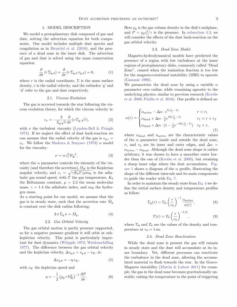
et al. 2009; Pinilla et al. 2016). Our profile is defined as:

α(r) =

αactive −∆α · e5( r

r1−1) r < r1

αdead + ∆α · 12e

10( rr2−1) r1 < r < r2

αdead + ∆α · (1− 12e−10( r

r2−1)) r2 < r,

(7)

where αdead and αactive are the characteristic values

of the α parameter inside and outside the dead zone,

r1 and r2 are its inner and outer edges, and ∆α =

αactive − αdead. Although the dead zone shape is rather

arbitrary, it was chosen to have a smoother outer bor-

der than the one of (Kretke et al. 2009), but retaining

a sharp inner edge where the dust accumulates. Fig-

ure 1 shows a diagram of the α profile, illustrating the

shape of the different intervals and its main components

to guide the reader with Eq. 7.

In order to maintain the steady state from Eq. 4 we de-

fine the initial surface density and temperature profiles

as follow:

Σg(r) = Σ0

(r

r0

)−1αactive

α(r), (8)

T (r) = T0

(r

r0

)−1/2

, (9)

where Σ0 and T0 are the values of the density and tem-

perature at r0 = 1 au.

2.4. Dead Zone Reactivation

While the dead zone is present the gas will remain

in steady state and the dust will accumulate at its in-

ner boundary. Yet, different processes can reactivate

the turbulence in the dead zone, allowing the accumu-

lated material to flush towards the star. In the Gravo-

Magneto instability (Martin & Lubow 2011) for exam-

ple, the gas in the dead zone becomes gravitationally un-

stable, raising the temperature to the point of triggering

4 Garate et al.

r1 r2r

dead

active

Figure 1. The diagram shows the shape of the α radialprofile for our dead zone model (in logarithmic scale). Thisconsists on three regions, the active inner zone limited by asharp decay at r1, the dead zone with a smooth rise towardsits outer edge around r2, and the outer active zone extendinguntil the outer boundary of the simulation.

the MRI, and finally producing an accretion outburst.

In our simulations we remain agnostic about the mech-

anism that causes the reactivation, and only set the re-

activation time tr arbitrarily, such that:

α(r, t > tr) = αactive. (10)

2.5. Dust Dynamics

The dust dynamics are governed by the gas motion

and the particle size. The time required for a particle of

size a and material density ρs to couple to the motion

of the gas is called the stopping time, and is defined as:

tstop =

√

π8ρsρg

acs

λmfp/a ≥ 4/9

29ρsρg

a2

νmolλmfp/a < 4/9,

(11)

with the mean free path λmfp = (nσH2)−1 (where n is

the number density, and σH2= 2× 10−15 cm2), and the

molecular viscosity νmol =√

2/πcsλmfp (following the

definitions in Birnstiel et al. 2010).

A more useful quantity to describe the dust-gas coupling

is the Stokes number (or dimensionless stopping time),

which is defined as:

St = tstopΩK . (12)

From this quantity we can quickly infer if a dust grain

is coupled (St 1) or decoupled (St 1) to the gas.

For the midplane this can be rewritten as:

St =

π2aρsΣg

λmfp/a ≥ 4/9

2π9

a2ρsλmfpΣg

λmfp/a < 4/9.(13)

The dust radial velocity is given in Nakagawa et al.

(1986); Takeuchi & Lin (2002) as:

vd =1

1 + St2vg,r+

2St

1 + St2∆vg,θ−Dd

Σg

Σd

∂

∂r(Σd

Σg). (14)

Here, the first term of the dust velocity is responsible

for small grains to move along with the gas, while the

second term is responsible for the dust to drift towards

the pressure maximum. The last term corresponds to

the dust diffusion contribution (see Birnstiel et al. 2010),

with Dd the dust diffusivity defined following Youdin &

Lithwick (2007) as:

Dd =ν

(1 + St2). (15)

The dust coagulation model is specified in Birnstiel et al.

(2010). Since our model focus on the inner regions of

the protoplanetary disks, the grain growth will always

be limited by the fragmentation barrier (Brauer et al.

2008), and the maximum grain size will be approxi-

mately:

Stfrag =1

3

v2frag

αc2s, (16)

where vfrag is the fragmentation velocity for dust parti-

cles (Birnstiel et al. 2012). For silicates this corresponds

to vfrag ≈ 1 m/s (Guttler et al. 2010).

2.6. Dust Back-reaction Effects

In protoplanetary disks, where the dust-to-gas ratio

ε = ρd/ρg is assumed to be 0.01, the effect of the dust

onto the gas is often neglected. However, in regions with

higher concentrations of solids, like in pressure bumps

(Pinilla et al. 2012), the angular momentum transfered

from the dust into the gas might be significant enough

to alter its dynamics.

Many authors have already derived and included the

effect of back-reaction (coupled with viscous evolution)

into numerical simulations, showing in which regimes it

should be considered (Tanaka et al. 2005; Garaud 2007;

Kretke et al. 2009; Kanagawa et al. 2017; Taki et al.

2016; Onishi & Sekiya 2017; Dipierro et al. 2018).

In this paper we include the dust back-reaction in one

of our simulations to study its impact on our model. To

do so, the gas velocities vg,r and ∆vg,θ are rewritten as

follows:

vg,r = Avν + 2BηvK , (17)

∆vg,θ =1

2Bvν −AηvK . (18)

The back-reaction coefficients A and B measure the de-

gree to which the gas dynamics are affected by the dust.

Dust accretion preceding an outburst? 5

These depend on the size distribution of the solids, and

the dust-to-gas ratio.

The formal definition and origin of back-reaction coef-

ficients can be found in the Appendix A, along with a

quick interpretation of them.

At this point we only want to remark that in the limit

where ε = 0 we obtain A = 1 and B = 0, recovering the

traditional velocities for the gas. When dust is present,

the value of A decreases and B increases. Thus, from

Eq. 17 we see that back-reaction slows down the viscous

evolution with the term Avν , and pushes the gas out-

ward with the term 2BηvK .

We find this contracted notation specially useful to sum-

marize the back-reaction contribution to the gas dy-

namic.

3. SIMULATION SETUP

In this section we describe the observational constrains

relevant for RW Aur A, the free parameters of our

model, and the setup of our 1D simulations using the

twopoppy (Birnstiel et al. 2012) and DustPy1 (Stamm-

ler & Birnstiel, in prep.) codes.

Our setup consists of three phases, the first phase sim-

ulates the dust accumulation at the dead zone, using a

global disk simulation over long timescales (∼ 105 yr),

but with a simplified and fast computational model for

the dust distribution using only two representative pop-

ulations. As the first phase only tracks the evolution

of the surface density, in a second phase we recover the

quasi-stationary particle size distribution at the inner

disk (r ≤ 5 au) by simulating the dust growth and frag-

mentation of multiple dust species. Finally, the third

phase simulates evolution of gas and dust (including co-

agulation, fragmentation, and transport) in the inner

disk after the dead zone is reactivated, to study the ac-

cretion of the accumulated material towards the star

over short timescales, and delivering the final results.

This setup is useful to save computational time, as we

are interested only in the inner disk after the dead zone

reactivation, but require the conditions given by the

global simulation.

3.1. Observational Constrains

RW Aur A is a young star with a stellar mass of M∗ =

1.4 M (Ghez et al. 1997; Woitas et al. 2001). The cir-

cumstellar disk has an estimated mass around Mdisk ≈4× 10−3 M (Andrews & Williams 2005), presents a

high accretion rate of M ≈ 4× 10−8−2× 10−7 M/yr

1 DustPy is a new Python code that solves the diffusion-advection of gas and dust, and the coagulation-fragmentation ofdust, based on the Birnstiel et al. (2010) algorithm.

(Hartigan et al. 1995; Ingleby et al. 2013; Facchini et al.

2016), and extends from a distance of ∼ 0.1 au (Akeson

et al. 2005; Eisner et al. 2007) until 58 au (Rodriguez

et al. 2018).

For the temperature profile we use T0 = 250 K, which

gives similar values to the Osterloh & Beckwith (1995)

profile in the inner regions of the disk for our choice of

slope.

Using these parameters, Eq. 3 and Eq. 4, we can con-

straint the values for the density and turbulence. From

the disk accretion rate, mass and size we infer the value

for the density Σ0 = 50 g/cm2 at r0 = 1 au, and the vis-

cous turbulence αactive = 0.1. These parameters yield

values of Mg = 5× 10−8 M/yr for the accretion rate,

and Mdisk = 2× 10−3 M for the disk mass (without

considering the accumulation excess in the dead zone).

The turbulence parameter αactive used in our simula-

tions is high, but necessary in order to account for the

high accretion rates measured.

3.2. Phase 1: Dust Concentration at the Dead Zone

In the first phase of our simulations we model the ac-

cumulation of dust in a disk with a dead zone, to obtain

the dust-to-gas ratio radial profile.

We use the TwoPopPy code to simulate a global pro-

toplanetary disk with two representative populations of

the dust species (details of the model can be found in

Birnstiel et al. 2012). We initialize our simulations using

Eq. 7, Eq. 8 and Eq. 9 for the α parameter, surface gas

density and temperature profiles, with the values pro-

vided by the observational constrains. For the dust-to-

gas ratio we assume an uniform initial value of ε = 0.01.

For this phase, the simulation domain goes from rin =

0.01 au to rout = 100 au, using nr = 500 radial grid

cells with logarithmic spacing. In the fiducial model,

the inner and outer boundaries of the dead zone are

r1 = 0.51 au, r2 = 10 au, with a depth of αdead = 10−4.

The simulation is evolved with this setup until the reac-

tivation time tr = 105yrs. Approximately at this point

the dust reaches its maximum accumulation at the inner

boundary of the dead zone, which will yield the maxi-

mum dust accretion rate in the next phase. Since the

gas is in steady state, we only evolve the dust in order

to minimize possible numerical errors. Inside the dead

zone, the gas phase is (marginally) gravitationally sta-

ble, with a Toomre parameter Q = csΩK/(πGΣg) & 1.5

(Toomre 1964). A low Q value in this region does not

conflict with the model, since the gravitational instabil-

ity is one of the mechanisms that can eventually reacti-

vate the dead zone.

The initial and final states of phase 1 are shown in Fig-

ure 2. During this phase the dust drifts towards the

6 Garate et al.

10 1 100 101

r (AU)

10 2

10 1

100

101

102

103

104

105

106

(g/c

m2)

Dust and Gas Densities

GasDust (t0 = 0 yrs)Dust (tr = 105 yrs)

Figure 2. Gas and dust surface density obtained fromTwoPopPy, at the beginning and at the end of the dustconcentration phase. The gas (red) remains in steady stateduring this phase. The dust is initialized with a dust-to gasratio of ε = 0.01 (dashed blue line). The dust component isevolved for 105 yrs (solid blue line) in which the dust con-centrates at the inner disk, reaching ε ≈ 0.24 at the innerboundary of the dead zone, and ε ≈ 0.16 inside this regionr < r1 = 0.51 au.

dead zone inner edge reaching values of ε = 0.24, and

concentrating 110 M⊕ between 0.51 - 0.6 au. Due to dif-

fusion, the dust concentration at the innermost part of

the disk also increases to values up to ε ≈ 0.16.

3.3. Phase 2: Dust Size Distribution at the Inner Disk

In the second phase we want to recover the dust size

distribution for multiple species, based on the dust-to-

gas ratio and disk conditions obtained in the previous

section.

We take the outcome of the TwoPopPy simulation as

the new initial conditions, and use the DustPy code to

solve the dust coagulation and fragmentation (following

the study of Birnstiel et al. 2010) at the inner disk,

while “freezing” the simulation exactly at the reactiva-

tion time t = tr, while the dead zone is still present (i.e.

still using Eq. 7).

The mass grid consists of nm = 141 logarithmic-spaced

cells, between m = 10−15− 105 g, at every radius. Since

in this phase we only care about the inner disk, we adjust

our simulation radial domain to be from rin = 0.05 au

to rout = 5 au. The radial grid is defined as follow:

• 25 linear-spaced grid cells at r = 0.05− 0.09 au,

• 120 logarithmic-spaced grid cells at r = 0.09 −1.0 au,

• 20 logarithmic-spaced grid cells at r = 1.0−5.0 au.

0.1 0.2 0.3 0.4 0.5 0.6 0.7r (AU)

10 4

10 3

10 2

10 1

100

101

Size

(cm

)

Time: tr + 0.0 yr

54321

01234

dust

[g/c

m2 ]

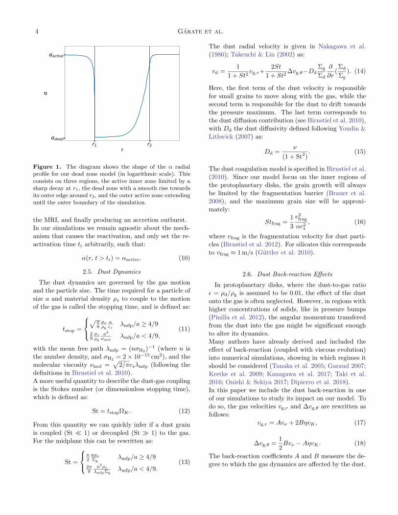
Figure 3. Dust distribution in the inner region of the proto-planetary disk immediately before the dead zone reactivation(t = tr). In the dead zone, where the turbulence and the col-lision speed of solids are lower, the dust particles can growto larger sizes (amax ∼ 1 cm) before reaching the fragmenta-tion limit. At the active zone, the particles are respectivelysmaller (amax ∼ 10µm). The inner edge of the dead zone(marked by the white line) presents a high concentration oflarge dust grains.

The innermost region is necessary to avoid numerical

problems with the inner boundary conditions. For opti-

mization purposes we also turn off coagulation for r <

0.09 au, since the growth and fragmentation timescales

are so short in this region that the simulation be-

comes computationally unfeasible. Moreover, accord-

ing to Akeson et al. (2005); Eisner et al. (2007) the

inner boundary of RW Aur A disk should be around

r ∼ 0.1 − 0.2 au. For these reasons all our analy-

sis will only focus on the region of interest between

r = 0.1− 1.0 au.

We interpolate the gas and dust surface densities from

the TwoPopPy simulation into the new grid, and use the

coagulation model of DustPy to obtain the correspond-

ing size distribution of the particles at t = tr for every

radius. The dust distribution obtained at this phase is

shown in Figure 3, where the grains adjust to the frag-

mentation limit in the dead and active zones.

3.4. Phase 3: Dead Zone Reactivation

For the final phase we simulate the evolution of dust

and gas in the inner disk, after the reactivation of the

dead zone (t > tr).

Once again we use the DustPy code, this time to solve

the advection of gas and dust, along with the dust

coagulation-fragmentation. We start this phase from the

conditions given at Section 3.3, using the same grid for

mass and radius, but now with the reactivated turbu-

Dust accretion preceding an outburst? 7

Table 1. Fiducial simulation parameters.

Parameter Value

Σ0 50 g/cm2

T0 250 K

r0 1 au

αactive 10−1

αdead 10−4

r1 0.51 au

r2 10 au

tr 105 yrs

Back-reaction Off

Table 2. Parameter variations.

Simulation Parameter Changed

Control Simulation tr = 0 yrs

Shallow Dead zone αdead = 10−3

Closer Inner Edge r1 = 0.25 au

Closer Outer Edge r2 = 4 au

Back-reaction On

lence following Eq. 10. We let the simulation evolve for

15 yrs, in which we expect that the material accumu-

lated at the inner boundary of the dead zone will drift

towards the star. The results of this phase on the ac-

cretion rate of gas and dust, as well as the final dust

distribution, will be shown in Section 4.2

3.5. Parameter Space

In Table 1 we summarize the parameters used for the

disk setup of our fiducial simulation. As the proper-

ties of the dead zone are free parameters, chosen to be

in a relevant range for the RW Aur dimming problem,

we also require to explore (even briefly) the parameter

space for these properties, and see how they affect the

final outcome of the simulations. We present five addi-

tional simulations, changing one parameter of the fidu-

cial model at a time, this way we explore the effect of

having: no initial dust accumulation at reactivation, dif-

ferent dead zone properties, and the expected effects of

back-reaction in the final result. The parameter changes

are described in Table 2.

4. RESULTS

In this section we show the results obtained on the

dust and gas dynamics after the “dead zone reactivation

2 The simulation data files and a plotting script are available inzenodo: doi.org/10.5281/zenodo.1495061.

0.1 0.2 0.3 0.4 0.5 0.6 0.7r (AU)

101

102

103

104

105

106

(g/c

m2)

DensityGasDust

0.1 0.2 0.3 0.4 0.5 0.6 0.7r (AU)

10 2

10 1

100

101

d/g

Dust-to-Gas RatioTime: tr + 15.0 yrTime: tr + 0 yr

Figure 4. The plots show the simulation state immediatelybefore the dead zone reactivation at t = tr (dashed lines), and15 yrs after it (solid lines). Top: Evolution of the gas (red)and dust (blue) surface densities. The initial state showsthe gas steady state profile and the accumulation of dust atthe inner boundary of the dead zone. After reactivation theaccumulation of dust flushes towards the star faster than thegas. Bottom: Dust-to-gas ratio evolution. At the initial statethe inner region presents an already high solid concentrationthanks to mixing at the dead zone boundary. During theflushing the dust-to-gas ratio reaches values of ε = 5 at someof the regions where the dust concentration arrived beforethe gas.

phase” (Section 3.4), including the final dust distribu-

tion, the dust-to-gas ratio at the inner boundary, and

accretion rates of dust and gas. We also study the im-

pact of the dead zone parameters on the final outcome,

to see if these results follow the expected behavior.

The gas and dust surface densities before and after the

reactivation are shown in Figure 4. The initial sur-

face density obtained from the first accumulation phase

shows a dust-to-gas ratio of ε = 0.24 at the dead zone

inner edge, and ε = 0.16 in the inner disk (r . 0.5 au).

8 Garate et al.

0.1 0.2 0.3 0.4 0.5 0.6 0.7r (AU)

10 4

10 3

10 2

10 1

100

101

Size

(cm

)

Time: tr + 0.05 yr

54321

01234

dust

[g/c

m2 ]

0.1 0.2 0.3 0.4 0.5 0.6 0.7r (AU)

10 4

10 3

10 2

10 1

100

101

Size

(cm

)

Time: tr + 15.0 yr

54321

01234

dust

[g/c

m2 ]

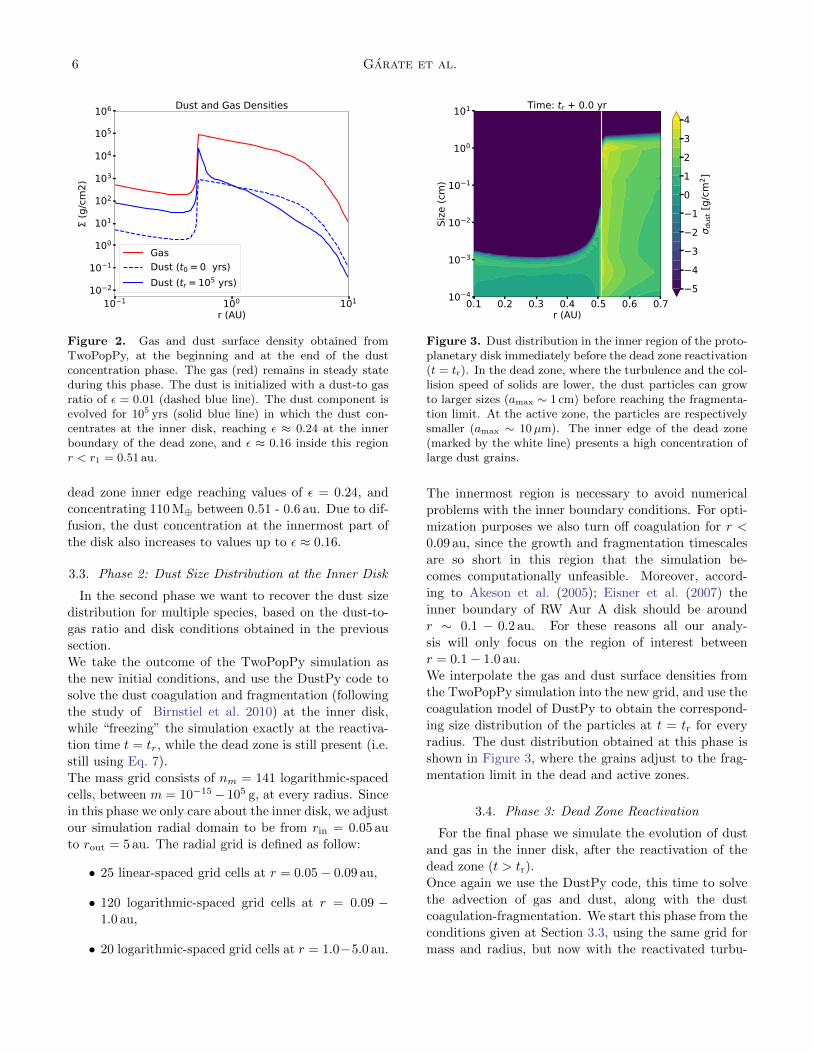
Figure 5. Dust distribution in the inner region of the proto-planetary disk after 0.05 and 15 yrs of the dead zone reactiva-tion. Top: The dust that was accumulated at the dead zonediffuses to the inner region within ∼ 10 collisional times, gen-erating high dust-to-gas concentrations. The original edge ofthe dead zone is marked in white. Bottom: Afterwards, thedust drifts towards the inner disk regions (r ∼ 0.1 − 0.2 au)within ∼ 15 yrs, while adjusting to the new fragmentationlimit.

After the reactivation (t > tr) the dust accumulated at

the dead zone is transported towards the inner regions

faster than the gas, reaching the inner boundary of the

disk (rin ∼ 0.1− 0.2 au (Akeson et al. 2005; Eisner et al.

2007)) in only 15 years.

Given that the surface density of dust at the dead zone

edge was higher than the gas surface density at the in-

ner regions, this leads to higher concentrations of dust

than gas after the reactivation (ε > 1). This should ob-

viously make the dust dynamically important to the gas

motion, however we shall see later in this section that as

the particles are too small (St < 10−3), the only impact

of dust back-reaction is to slow down the dust and gas

evolution. Therefore no instabilities are generated and

0 2 4 6 8 10 12 14Time (yr)

10 8

10 7

10 6

10 5

M (M

/yr)

Accretion rate at r: 0.15 AUGasDust

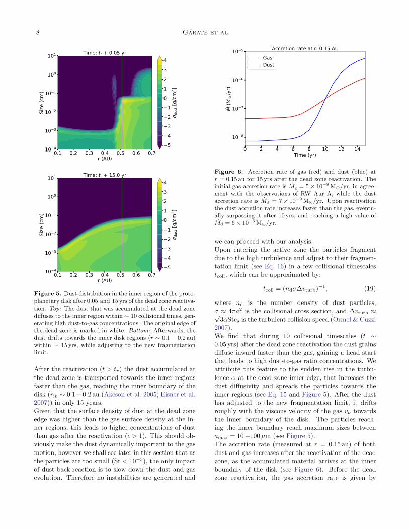
Figure 6. Accretion rate of gas (red) and dust (blue) atr = 0.15 au for 15 yrs after the dead zone reactivation. Theinitial gas accretion rate is Mg = 5 × 10−8 M/yr, in agree-ment with the observations of RW Aur A, while the dustaccretion rate is Md = 7 × 10−9 M/yr. Upon reactivationthe dust accretion rate increases faster than the gas, eventu-ally surpassing it after 10 yrs, and reaching a high value ofMd = 6 × 10−6 M/yr.

we can proceed with our analysis.

Upon entering the active zone the particles fragment

due to the high turbulence and adjust to their fragmen-

tation limit (see Eq. 16) in a few collisional timescales

tcoll, which can be approximated by:

tcoll = (ndσ∆vturb)−1, (19)

where nd is the number density of dust particles,

σ ≈ 4πa2 is the collisional cross section, and ∆vturb ≈√3αStcs is the turbulent collision speed (Ormel & Cuzzi

2007).

We find that during 10 collisional timescales (t ∼0.05 yrs) after the dead zone reactivation the dust grains

diffuse inward faster than the gas, gaining a head start

that leads to high dust-to-gas ratio concentrations. We

attribute this feature to the sudden rise in the turbu-

lence α at the dead zone inner edge, that increases the

dust diffusivity and spreads the particles towards the

inner regions (see Eq. 15 and Figure 5). After the dust

has adjusted to the new fragmentation limit, it drifts

roughly with the viscous velocity of the gas vν towards

the inner boundary of the disk. The particles reach-

ing the inner boundary reach maximum sizes between

amax = 10−100µm (see Figure 5).

The accretion rate (measured at r = 0.15 au) of both

dust and gas increases after the reactivation of the dead

zone, as the accumulated material arrives at the inner

boundary of the disk (see Figure 6). Before the dead

zone reactivation, the gas accretion rate is given by

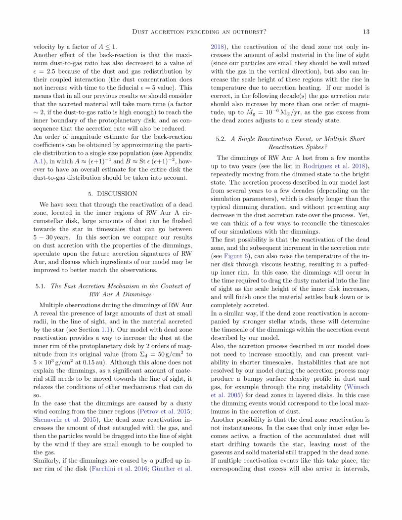
Dust accretion preceding an outburst? 9

the steady state solution with Mg = 5× 10−8 M/yr,

similar to the observational value of (Facchini et al.

2016; Ingleby et al. 2013), and the dust accretion rate is

Md = 7× 10−9 M/yr, this value comes from the dust

diffusing into the inner disk during the concentration

phase.

After the dead zone reactivation the dust concentra-

tion moves inwards, and the accretion rate at the inner

boundary of the disk becomes dominated by the dust, to

the point of surpassing that of the gas. This high sup-

ply of solid material, with Md = 6× 10−6 M/yr could

cause hot dust and metallicity features of RW Aur A

(Shenavrin et al. 2015; Gunther et al. 2018), and provide

an ideal environment for the dimmings to occur (see Sec-

tion 5.1). At this point we also note that the accretion

rate of gas has increased up to Mg = 10−6 M/yr.

In Section 5 we will discuss how the high accretion of

solids could cause the dimmings in the context of previ-

ous proposed mechanisms (dusty winds, puffed-up inner

disk rim, etc), and if we can expect future accretion

signatures from the gas. In the following subsections,

we study the effect of the simulation parameters on the

dust dynamics.

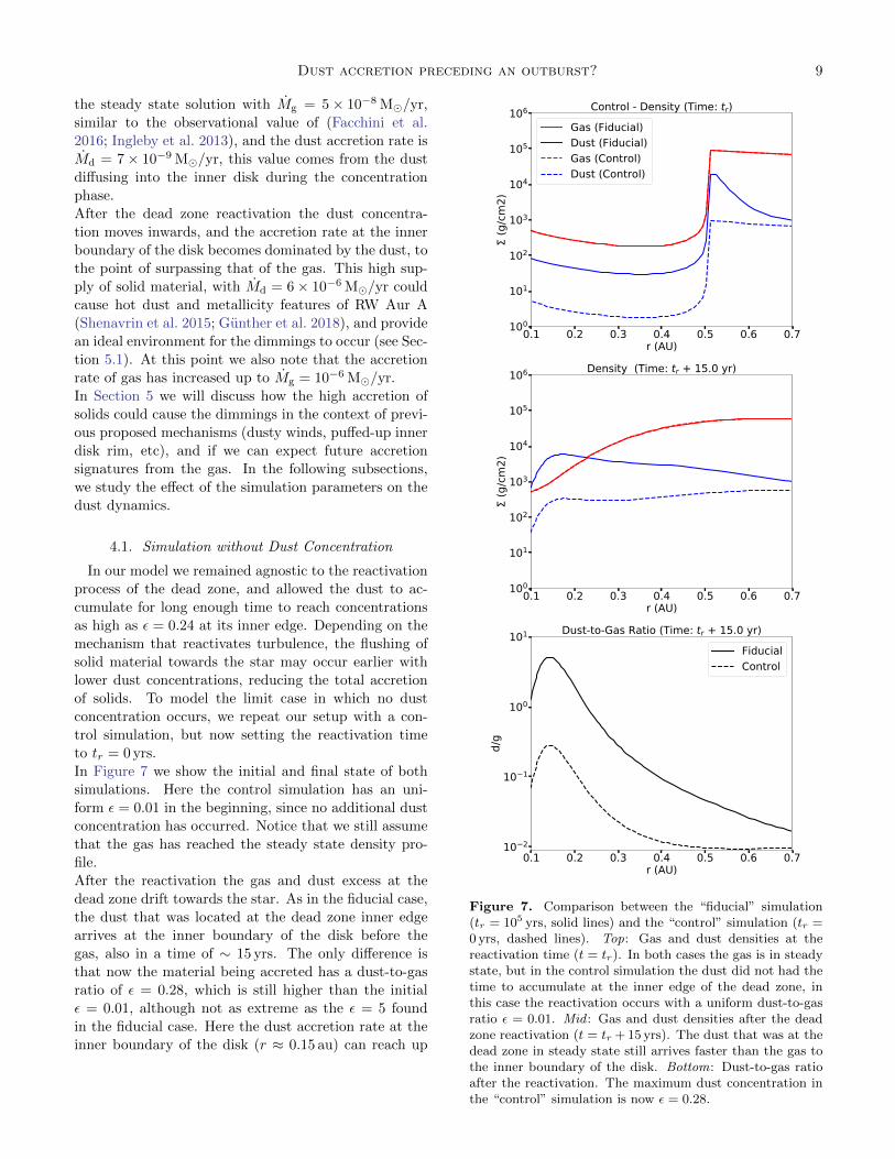
4.1. Simulation without Dust Concentration

In our model we remained agnostic to the reactivation

process of the dead zone, and allowed the dust to ac-

cumulate for long enough time to reach concentrations

as high as ε = 0.24 at its inner edge. Depending on the

mechanism that reactivates turbulence, the flushing of

solid material towards the star may occur earlier with

lower dust concentrations, reducing the total accretion

of solids. To model the limit case in which no dust

concentration occurs, we repeat our setup with a con-

trol simulation, but now setting the reactivation time

to tr = 0 yrs.

In Figure 7 we show the initial and final state of both

simulations. Here the control simulation has an uni-

form ε = 0.01 in the beginning, since no additional dust

concentration has occurred. Notice that we still assume

that the gas has reached the steady state density pro-

file.

After the reactivation the gas and dust excess at the

dead zone drift towards the star. As in the fiducial case,

the dust that was located at the dead zone inner edge

arrives at the inner boundary of the disk before the

gas, also in a time of ∼ 15 yrs. The only difference is

that now the material being accreted has a dust-to-gas

ratio of ε = 0.28, which is still higher than the initial

ε = 0.01, although not as extreme as the ε = 5 found

in the fiducial case. Here the dust accretion rate at the

inner boundary of the disk (r ≈ 0.15 au) can reach up

0.1 0.2 0.3 0.4 0.5 0.6 0.7r (AU)

100

101

102

103

104

105

106

(g/c

m2)

Control - Density (Time: tr)Gas (Fiducial)Dust (Fiducial)Gas (Control)Dust (Control)

0.1 0.2 0.3 0.4 0.5 0.6 0.7r (AU)

100

101

102

103

104

105

106

(g/c

m2)

Density (Time: tr + 15.0 yr)

0.1 0.2 0.3 0.4 0.5 0.6 0.7r (AU)

10 2

10 1

100

101

d/g

Dust-to-Gas Ratio (Time: tr + 15.0 yr)FiducialControl

Figure 7. Comparison between the “fiducial” simulation(tr = 105 yrs, solid lines) and the “control” simulation (tr =0 yrs, dashed lines). Top: Gas and dust densities at thereactivation time (t = tr). In both cases the gas is in steadystate, but in the control simulation the dust did not had thetime to accumulate at the inner edge of the dead zone, inthis case the reactivation occurs with a uniform dust-to-gasratio ε = 0.01. Mid : Gas and dust densities after the deadzone reactivation (t = tr + 15 yrs). The dust that was at thedead zone in steady state still arrives faster than the gas tothe inner boundary of the disk. Bottom: Dust-to-gas ratioafter the reactivation. The maximum dust concentration inthe “control” simulation is now ε = 0.28.

10 Garate et al.

to Md = 3× 10−7 M/yr.

From here we learn that the dust arrival time at the in-

ner boundary does not depend on the amount of solids

accumulated at the dead zone inner edge, and that upon

reactivation the accreted material will still carry a high

concentration of solids.

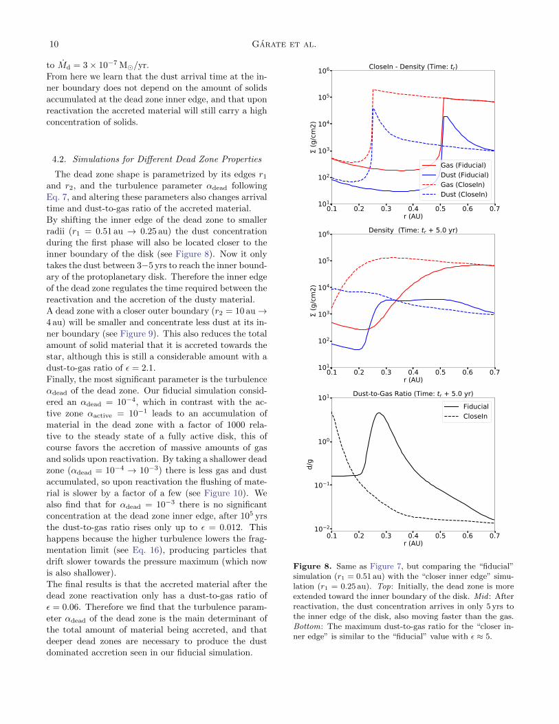
4.2. Simulations for Different Dead Zone Properties

The dead zone shape is parametrized by its edges r1

and r2, and the turbulence parameter αdead following

Eq. 7, and altering these parameters also changes arrival

time and dust-to-gas ratio of the accreted material.

By shifting the inner edge of the dead zone to smaller

radii (r1 = 0.51 au → 0.25 au) the dust concentration

during the first phase will also be located closer to the

inner boundary of the disk (see Figure 8). Now it only

takes the dust between 3−5 yrs to reach the inner bound-

ary of the protoplanetary disk. Therefore the inner edge

of the dead zone regulates the time required between the

reactivation and the accretion of the dusty material.

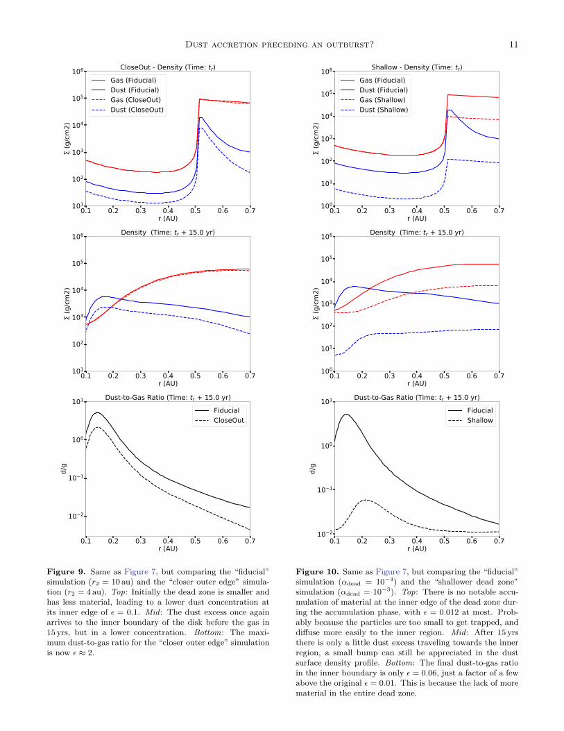
A dead zone with a closer outer boundary (r2 = 10 au→4 au) will be smaller and concentrate less dust at its in-

ner boundary (see Figure 9). This also reduces the total

amount of solid material that it is accreted towards the

star, although this is still a considerable amount with a

dust-to-gas ratio of ε = 2.1.

Finally, the most significant parameter is the turbulence

αdead of the dead zone. Our fiducial simulation consid-

ered an αdead = 10−4, which in contrast with the ac-

tive zone αactive = 10−1 leads to an accumulation of

material in the dead zone with a factor of 1000 rela-

tive to the steady state of a fully active disk, this of

course favors the accretion of massive amounts of gas

and solids upon reactivation. By taking a shallower dead

zone (αdead = 10−4 → 10−3) there is less gas and dust

accumulated, so upon reactivation the flushing of mate-

rial is slower by a factor of a few (see Figure 10). We

also find that for αdead = 10−3 there is no significant

concentration at the dead zone inner edge, after 105 yrs

the dust-to-gas ratio rises only up to ε = 0.012. This

happens because the higher turbulence lowers the frag-

mentation limit (see Eq. 16), producing particles that

drift slower towards the pressure maximum (which now

is also shallower).

The final results is that the accreted material after the

dead zone reactivation only has a dust-to-gas ratio of

ε = 0.06. Therefore we find that the turbulence param-

eter αdead of the dead zone is the main determinant of

the total amount of material being accreted, and that

deeper dead zones are necessary to produce the dust

dominated accretion seen in our fiducial simulation.

0.1 0.2 0.3 0.4 0.5 0.6 0.7r (AU)

101

102

103

104

105

106

(g/c

m2)

CloseIn - Density (Time: tr)

Gas (Fiducial)Dust (Fiducial)Gas (CloseIn)Dust (CloseIn)

0.1 0.2 0.3 0.4 0.5 0.6 0.7r (AU)

101

102

103

104

105

106

(g/c

m2)

Density (Time: tr + 5.0 yr)

0.1 0.2 0.3 0.4 0.5 0.6 0.7r (AU)

10 2

10 1

100

101

d/g

Dust-to-Gas Ratio (Time: tr + 5.0 yr)FiducialCloseIn

Figure 8. Same as Figure 7, but comparing the “fiducial”simulation (r1 = 0.51 au) with the “closer inner edge” simu-lation (r1 = 0.25 au). Top: Initially, the dead zone is moreextended toward the inner boundary of the disk. Mid : Afterreactivation, the dust concentration arrives in only 5 yrs tothe inner edge of the disk, also moving faster than the gas.Bottom: The maximum dust-to-gas ratio for the “closer in-ner edge” is similar to the “fiducial” value with ε ≈ 5.

Dust accretion preceding an outburst? 11

0.1 0.2 0.3 0.4 0.5 0.6 0.7r (AU)

101

102

103

104

105

106 (g

/cm

2)CloseOut - Density (Time: tr)

Gas (Fiducial)Dust (Fiducial)Gas (CloseOut)Dust (CloseOut)

0.1 0.2 0.3 0.4 0.5 0.6 0.7r (AU)

101

102

103

104

105

106

(g/c

m2)

Density (Time: tr + 15.0 yr)

0.1 0.2 0.3 0.4 0.5 0.6 0.7r (AU)

10 2

10 1

100

101

d/g

Dust-to-Gas Ratio (Time: tr + 15.0 yr)FiducialCloseOut

Figure 9. Same as Figure 7, but comparing the “fiducial”simulation (r2 = 10 au) and the “closer outer edge” simula-tion (r2 = 4 au). Top: Initially the dead zone is smaller andhas less material, leading to a lower dust concentration atits inner edge of ε = 0.1. Mid : The dust excess once againarrives to the inner boundary of the disk before the gas in15 yrs, but in a lower concentration. Bottom: The maxi-mum dust-to-gas ratio for the “closer outer edge” simulationis now ε ≈ 2.

0.1 0.2 0.3 0.4 0.5 0.6 0.7r (AU)

100

101

102

103

104

105

106

(g/c

m2)

Shallow - Density (Time: tr)Gas (Fiducial)Dust (Fiducial)Gas (Shallow)Dust (Shallow)

0.1 0.2 0.3 0.4 0.5 0.6 0.7r (AU)

100

101

102

103

104

105

106

(g/c

m2)

Density (Time: tr + 15.0 yr)

0.1 0.2 0.3 0.4 0.5 0.6 0.7r (AU)

10 2

10 1

100

101

d/g

Dust-to-Gas Ratio (Time: tr + 15.0 yr)FiducialShallow

Figure 10. Same as Figure 7, but comparing the “fiducial”simulation (αdead = 10−4) and the “shallower dead zone”simulation (αdead = 10−3). Top: There is no notable accu-mulation of material at the inner edge of the dead zone dur-ing the accumulation phase, with ε = 0.012 at most. Prob-ably because the particles are too small to get trapped, anddiffuse more easily to the inner region. Mid : After 15 yrsthere is only a little dust excess traveling towards the innerregion, a small bump can still be appreciated in the dustsurface density profile. Bottom: The final dust-to-gas ratioin the inner boundary is only ε = 0.06, just a factor of a fewabove the original ε = 0.01. This is because the lack of morematerial in the entire dead zone.

12 Garate et al.

4.3. Simulation with Dust Back-reaction

In all our results until this point we have neglected

the back-reaction of dust to the gas, however for the

dust-to-gas ratios presented during the dead zone reac-

tivation (ε & 1) this effect should be relevant. In this

section we study its impact to see if our previous results

remain valid.

First, we should mention that in this setup we only con-

sider the back-reaction in the “reactivation phase”, and

assume that the dust will still accumulate at the inner

edge of the dead zone even if back-reactions are con-

sidered. This is still justified since our particles are

too small (St < 10−3) to cause any perturbation be-

yond slowing down the concentration process and we

can be infer it also by studying the single dust species

scenario described in the Appendix A.1. Studies of On-

ishi & Sekiya (2017) also showed that the back-reaction

still allows the dust to accumulate at pressure maxima,

and that the dust traps do not self-destruct by this ef-

fect when taking into account the vertical distribution

of solids.

For the reactivation phase we implement the gas ve-

locities as described by equations Eq. 17 and Eq. 18.

In the radial direction, the gas velocity now consist of

two terms modulated by the back-reaction coefficients

0 < A,B < 1, the term Avν is slowing down the viscous

evolution of the gas respect to the default value vν , and

the term 2BηvK is pushing the gas in the direction op-

posite to the pressure gradient.

Since the vertical distribution of particles is not exactly

the same as the gas, the effect of the back-reaction is also

not uniform in the vertical direction, the importance of

this point is shown in Dipierro et al. (2018); Onishi &

Sekiya (2017). To account for the vertical effect of back-

reactions in our 1D simulations we take the vertically

averaged velocity for the dust and gas, weighted by the

mass density to conserve the total flux. The details for

this implementation can also be found in the Appendix

A.2.

In Figure 11 we show a comparison between the “fidu-

cial” and “back-reaction” simulations 15 years after the

dead zone reactivation. When the back-reaction is con-

sidered the most notable effect is the slowing down of

the accretion of material by a factor of ∼ 2. While the

dust particles in the “fiducial” simulation take 15 years

to reach the inner boundary of the disk, in the “back-

reaction” simulation they need 30 years instead.

The reason why no further effects are observed is that

the high turbulence causes fragmentation of the parti-

cles to smaller sizes (as seen in Figure 5), where they

are unable to “push” the gas backwards (i.e. the term

B → 0), and are only able to reduce the gas viscous

0.1 0.2 0.3 0.4 0.5 0.6 0.7r (AU)

101

102

103

104

105

106

(g/c

m2)

Backreaction - Density (Time: tr)Gas (Fiducial)Dust (Fiducial)Gas (Backreaction)Dust (Backreaction)

0.1 0.2 0.3 0.4 0.5 0.6 0.7r (AU)

101

102

103

104

105

106

(g/c

m2)

Density (Time: tr + 15.0 yr)

0.1 0.2 0.3 0.4 0.5 0.6 0.7r (AU)

10 2

10 1

100

101

d/g

Dust-to-Gas Ratio (Time: tr + 15.0 yr)FiducialBackreaction

Figure 11. Same as Figure 7, but comparing the “fiducial”simulation and the “back-reaction” simulation. Top: Bothsimulations start at the reactivation time with the same ini-tial conditions. Mid : When back-reaction is considered, theevolution of the dust and gas component is slower than in thefiducial case. This is because the high dust concentrationsslow down the viscous evolution of the gas, which in turnalso slows down the drifting of the dust towards the innerdisk. Bottom: Both the simulation with and without back-reaction present a high concentration of dust in the accretedmaterial, yet in the case with back-reaction the bulk of dustreaches a radii of only r = 0.22 au in 15 years, while the dustin the fiducial simulation is already at r = 0.15 au.

Dust accretion preceding an outburst? 13

velocity by a factor of A ≤ 1.

Another effect of the back-reaction is that the maxi-

mum dust-to-gas ratio has also decreased to a value of

ε = 2.5 because of the dust and gas redistribution by

their coupled interaction (the dust concentration does

not increase with time to the fiducial ε = 5 value). This

means that in all our previous results we should consider

that the accreted material will take more time (a factor

∼ 2, if the dust-to-gas ratio is high enough) to reach the

inner boundary of the protoplanetary disk, and as con-

sequence that the accretion rate will also be reduced.

An order of magnitude estimate for the back-reaction

coefficients can be obtained by approximating the parti-

cle distribution to a single size population (see Appendix

A.1), in which A ≈ (ε+1)−1 and B ≈ St ε (ε+1)−2, how-

ever to have an overall estimate for the entire disk the

dust-to-gas distribution should be taken into account.

5. DISCUSSION

We have seen that through the reactivation of a dead

zone, located in the inner regions of RW Aur A cir-

cumstellar disk, large amounts of dust can be flushed

towards the star in timescales that can go between

5 − 30 years. In this section we compare our results

on dust accretion with the properties of the dimmings,

speculate upon the future accretion signatures of RW

Aur, and discuss which ingredients of our model may be

improved to better match the observations.

5.1. The Fast Accretion Mechanism in the Context of

RW Aur A Dimmings

Multiple observations during the dimmings of RW Aur

A reveal the presence of large amounts of dust at small

radii, in the line of sight, and in the material accreted

by the star (see Section 1.1). Our model with dead zonereactivation provides a way to increase the dust at the

inner rim of the protoplanetary disk by 2 orders of mag-

nitude from its original value (from Σd = 50 g/cm2 to

5× 103 g/cm2 at 0.15 au). Although this alone does not

explain the dimmings, as a significant amount of mate-

rial still needs to be moved towards the line of sight, it

relaxes the conditions of other mechanisms that can do

so.

In the case that the dimmings are caused by a dusty

wind coming from the inner regions (Petrov et al. 2015;

Shenavrin et al. 2015), the dead zone reactivation in-

creases the amount of dust entangled with the gas, and

then the particles would be dragged into the line of sight

by the wind if they are small enough to be coupled to

the gas.

Similarly, if the dimmings are caused by a puffed up in-

ner rim of the disk (Facchini et al. 2016; Gunther et al.

2018), the reactivation of the dead zone not only in-

creases the amount of solid material in the line of sight

(since our particles are small they should be well mixed

with the gas in the vertical direction), but also can in-

crease the scale height of these regions with the rise in

temperature due to accretion heating. If our model is

correct, in the following decade(s) the gas accretion rate

should also increase by more than one order of magni-

tude, up to Mg = 10−6 M/yr, as the gas excess from

the dead zones adjusts to a new steady state.

5.2. A Single Reactivation Event, or Multiple Short

Reactivation Spikes?

The dimmings of RW Aur A last from a few months

up to two years (see the list in Rodriguez et al. 2018),

repeatedly moving from the dimmed state to the bright

state. The accretion process described in our model last

from several years to a few decades (depending on the

simulation parameters), which is clearly longer than the

typical dimming duration, and without presenting any

decrease in the dust accretion rate over the process. Yet,

we can think of a few ways to reconcile the timescales

of our simulations with the dimmings.

The first possibility is that the reactivation of the dead

zone, and the subsequent increment in the accretion rate

(see Figure 6), can also raise the temperature of the in-

ner disk through viscous heating, resulting in a puffed-

up inner rim. In this case, the dimmings will occur in

the time required to drag the dusty material into the line

of sight as the scale height of the inner disk increases,

and will finish once the material settles back down or is

completely accreted.

In a similar way, if the dead zone reactivation is accom-

panied by stronger stellar winds, these will determine

the timescale of the dimmings within the accretion event

described by our model.

Also, the accretion process described in our model does

not need to increase smoothly, and can present vari-

ability in shorter timescales. Instabilities that are not

resolved by our model during the accretion process may

produce a bumpy surface density profile in dust and

gas, for example through the ring instability (Wunsch

et al. 2005) for dead zones in layered disks. In this case

the dimming events would correspond to the local max-

imums in the accretion of dust.

Another possibility is that the dead zone reactivation is

not instantaneous. In the case that only inner edge be-

comes active, a fraction of the accumulated dust will

start drifting towards the star, leaving most of the

gaseous and solid material still trapped in the dead zone.

If multiple reactivation events like this take place, the

corresponding dust excess will also arrive in intervals,

14 Garate et al.

with a frequency depending on the reactivation mech-

anism. In this case the dimmings would start when a

spike of dust accretion arrives to the inner edge, and

end once it decreases back to its steady state value. To

improve our model we would need to resolve the ther-

mal and gravitational instabilities that can reactivate

the dead zone (Martin & Lubow 2011).

Finally, azimuthal asymmetries in the inner disk (such

as vortices) may also add variability to the accretion

process, but these are not considered by our model.

A further monitoring of the metallicity of the accreted

material would help understand the nature of the dust

accretion process and the mechanism that drags the

dust into the line of sight. If the dust accretion contin-

ues delivering material to the star, independently of the

dimmings, then the metallicity should remain high even

after the luminosity returns to the bright state. Oth-

erwise, if the rise in metallicity keeps correlating with

the dimmings (as in Gunther et al. 2018), the dimmings

could be an outcome of the sudden increase in the dust

accretion (although of course, correlation does not imply

causality).

5.3. Validity of the Dead Zone Model

Our results showed that the exact values of dust ac-

cretion rate and timescales depend sensitively on the

parameters used for the dead zone. A dead zone inner

edge closer to the inner boundary of the disk reduces

the timescale of the process, a closer outer edge reduces

the total mass of the dead zone, and the turbulence pa-

rameter αdead and the reactivation time determine the

amount of dust that can be trapped and flushed towards

the star. In addition, the shape of the dead zone profile

also affects dust and gas surface density profiles, and a

proper modeling of the gas turbulence would be required

to obtain their final distributions after the dead zone re-

activation.

With this amount of free parameters, our simulations

provide more a qualitative scenario than quantitative

predictions. Further constrains are necessary to deter-

mine how relevant the reactivation of a dead zone can

be for RW Aur A dimmings. The first step is of course

to find the mechanism that puts the required amounts

of dust in the line of sight, and obtain an estimate of

the required dust surface density at the inner disk (not

only in the line of sight) to produce this phenomena.

In parallel, any signature of enhanced gas accretion rate

in the following years would speak in favor of the dead

zone reactivation mechanism as one of the drivers of the

dimmings.

Additionally, constrains on the properties of the inner

disk would limit the parameter space described. In par-

ticular, the mass in the inner 10 au of RW Aur A disk

would be useful to constrain the outer edge and turbu-

lence parameter of the dead zone, and with them the

amount of material that can be thrown to the star.

5.3.1. The Dead Zone as an Accretion Reservoir

One point that speaks in favor of our model is its po-

tential to sustain the large accretion rates of RW Aur for

extended periods of time. Considering only the observed

values for the disk mass and the accretion rate, the max-

imum lifetime of RW Aur would be of Mg/Mg ∼ 104 -

105 yrs which is too short for a T Tauri star.

Rosotti et al. (2017) defined the dimensionless accretion

parameter:

ηacc = τ∗M/Mdisk, (20)

with τ∗ the age of the star, that indicates if the proper-

ties of a disk are consistent the steady state accretion, in

which case it follows ηacc . 1. The RW Aur A is around

5 Myr old (Ghez et al. 1997) and presents an accretion

parameter of ηacc ≈ 60, indicating either that the disk

is not in steady state, or that the observed disk mass is

underestimated.

In our model, the dead zone provides a reservoir of ma-

terial able to sustain the detected accretion rates for

around 2Myrs (considering the parameters of our fidu-

cial simulation), which is close to the estimated age

of the star. At the same time, at high densities the

dusty material would be optically thick, remaining hid-

den from the mm observations used to measure the disk

mass.

5.3.2. Another Free Parameter for Dust Growth?

In our model we considered that the turbulent α

that limits dust growth by fragmentation (Eq. 16), is

the same that drives the viscous evolution of the gas

(Eq. 3), yet recent models explore the case with two in-

dependent α values for each process (e.g., Carrera et al.

2017). For our model, using a single α value means that

particles reach bigger sizes while they remain in the

dead zone, and fragment to smaller sizes in the active

region.

Allowing two independent alpha values would allow the

formation of large particles in the active region. These

larger particles drift faster, but also exert a stronger

back-reaction on the gas. The “pushing” back-reaction

coefficient B is roughly proportional to the particle size

(see Appendix A.1), and at the high dust-to-gas ratios

found during the dead zone reactivation, it could be

strong enough to generate density bumps in the gas, or

even trigger the streaming instability for particles with

large enough Stokes number (Youdin & Goodman 2005).

Dust accretion preceding an outburst? 15

6. SUMMARY

In this work we studied a new mechanism that can

increase the concentration of solids in the inner regions

of a protoplanetary disk in timescales of ∼ 10 years,

through the reactivation of a dead zone.

This study was motivated by the recent dimmings of

RW Aur A, which present a high concentration dust

in the line of sight (Antipin et al. 2015; Schneider

et al. 2015), and an increased emission from hot grains

coming from the inner regions of the protoplanetary

disk(Shenavrin et al. 2015), and subsequently observed

super-solar metallicity of the accreted material(Gunther

et al. 2018).

Using 1D simulations to model the circumstellar disk of

RW Aur A, we find that the dust grains accumulate at

the inner edge of the dead zone, which acts as a dust

trap, reaching concentrations of ε ≈ 0.25. When the tur-

bulence in this region is reactivated, the excess of gas

and dust is released from the dead zone and advected

towards the star. By effect of dust diffusion and gas

drag, the dust component can reach the inner boundary

of the protoplanetary disk before the gas component,

producing high dust concentrations of ε ≈ 5.

The accretion rate of solids increases from Md =

7× 10−9 M/yr to 6× 10−6 M/yr in only 15 years.

This scenario can provide an ideal environment for other

mechanisms, such as stellar winds (Petrov et al. 2015;

Shenavrin et al. 2015) or a puffed up inner rim (e.g.,

Facchini et al. 2016; Gunther et al. 2018), to transport

the required amount of solid material into the line of

sight and cause the dimmings, although further studies

are required to link the surface density at the midplane

with the measured dust concentrations.

Additionally, our simulations predict that in the follow-

ing decade(s) the gas accretion rate should also rise by

an order of magnitude, from Mg = 5× 10−8 M/yr to

10−6 M/yr if the dead zone reactivation is the mecha-

nism transporting dust towards the disk inner region.

ACKNOWLEDGMENTS

We would like to thank S. Facchini, and also the

anonymous referee, for their useful comments that im-

proved the extent of this work. M. G., T. B., and

S. M. S. acknowledge funding from the European Re-

search Council (ERC) under the European Unions Hori-

zon 2020 research and innovation programme under

grant agreement No 714769 and funding by the Deutsche

Forschungsgemeinschaft (DFG, German Research Foun-

dation) Ref no. FOR 2634/1. HMG was supported

by the National Aeronautics and Space Administration

through Chandra Award Number GO6-17021X issued

by the Chandra X-ray Observatory Center, which is op-

erated by the Smithsonian Astrophysical Observatory

for and on behalf of the National Aeronautics Space Ad-

ministration under contract NAS8-03060.

APPENDIX

A. DETAILS OF DUST BACK-REACTION

The gas and dust velocities incorporating the back-reaction of the dust into the gas is obtained from the momentum

conservation equations shown in Nakagawa et al. (1986), and considering the force exerted by the multiple species of

dust as in (Tanaka et al. 2005). In this case the gas feels the drag force of multiple species, the pressure force, the

viscous force, and the stellar gravity, while the dust only feels the stellar gravity and the drag force from the gas.

The momentum equations for the gas and dust then are respectively:

dvg

dt= −

∫(vg − vd)

tstop

ρd(m)

ρgdm− GM∗

r2r− 1

ρg

∂P

∂rr + fν θ, (A1)

dvd

dt= − (vd − vg)

tstop− GM∗

r2r, (A2)

where the viscous force contribution in the azimuthal direction can be conveniently written as fν = ΩKvν/2.

Solving this system of equations for the steady state gives the radial and azimuthal velocities for gas as shown in

Eq. 17, Eq. 18, and the radial velocity for the dust given by Eq. 14.

The back-reaction coefficients A, B are defined as:

A =X + 1

Y 2 + (X + 1)2, (A3)

B =Y

Y 2 + (X + 1)2, (A4)

16 Garate et al.

with X and Y following the notation of Okuzumi et al. (2012):

X =

∫1

1 + St2

ρd(m)

ρgdm, (A5)

Y =

∫St

1 + St2

ρd(m)

ρgdm. (A6)

The X,Y integrals come from the contribution of the multiple dust species at the momentum conservation equations

described by Tanaka et al. (2005). Here ρd(m) is the dust volume density per mass, and the dust-to-gas ratio at each

mass bin ε(m) = (ρd(m)/ρg)dm determines the contribution of each particle species to the final result.

To summarize the effect of back-reactions on the gas, we can understand the coefficient A as a “smoothing” factor

and the coefficient B as a “pushing” factor. The “smoothing” factor A reduces the effect of the viscous force in the

radial velocity (slowing down the accretion), and reduces the effect of the pressure gradient in the azimuthal velocity

(making the gas orbital velocity more keplerian). The “pushing” factor B on the other hand, pushes the gas in the

direction opposite to the pressure gradient in the radial direction (with the term 2BηvK), and slows down the orbital

velocity (with the term Bvν/2). Which term dominates in the radial evolution of dust and gas will also depend on the

magnitude of the pressure gradient and the viscosity (Dipierro et al. 2018).

A.1. Single Species Analysis

The expressions for A and B are difficult to study by eye, but we can consider the case with a single species of

particles to simplify subsequent analysis. In this case the integrals X and Y become:

Xsingle =1

1 + St2 ε, (A7)

Ysingle =St

1 + St2 ε. (A8)

The back-reaction coefficients now have a simple expression that only depends on the Stokes number and the dust-to-

gas ratio:

Asingle =ε+ 1 + St2

(ε+ 1)2 + St2 , (A9)

Bsingle =εSt

(ε+ 1)2 + St2 . (A10)

From these equations we can start noticing some interesting values for A and B:

• 0 < A,B < 1

• The limit without particles ε→ 0, recovers the traditional gas velocities:

– A→ 1

– B → 0

• The limit with small particles, assuming St << 1 gives:

– A ≈ (ε+ 1)−1

– B ≈ St ε (ε+ 1)−2

The last case is applicable to our simulations, since we have high dust-to-gas ratios of small particles only, in this case

we reach the limit of B ≈ 0 and A ≈ (1 + ε)−1, and therefore we only care about the slowing effect of the particles on

the gas.

Dust accretion preceding an outburst? 17

A.2. Considering the Vertical Structure

The dust-to-gas ratio is not necessarily constant in the vertical direction. As shown by Okuzumi et al. (2012);

Dipierro et al. (2018) this might have an impact in the effects of the back-reaction, since the velocities of the gas and

dust will experience a different force in the different layers of the disk.

We assume that both the gas and dust densities are distributed as a Gaussian in the vertical direction:

ρg(z) =Σg√2πHg

exp(− z2

2H2g

), (A11)

ρd(m, z)dm =Σd(m)√2πHd(m)

exp(− z2

2H2d(m)

). (A12)

Here ρd(m, z)dm is the volume density of the particles in the mass bin m at a height z, and Σd(m) is the surface

density of particles at the mass bin m. Hg and Hd(m) are the scale heights of the gas and the dust particles with

mass m, respectively defined as:

Hg =cs

ΩK, (A13)

Hd(m) = Hg ·min(1,

√α

min(St, 1/2)(1 + St2)), (A14)

the last equation coming from Birnstiel et al. (2010), that tells us that bigger particles are more concentrated towards

the midplane, while small particles are distributed like the gas.

With the vertical distribution of gas and dust we can obtain the mass weighted average radial velocity vg,d, defined to

conserve the radial mass flux, as:

Σg,dvg,d =

∫ +∞

−∞ρg,d(z)vg,d(z)dz. (A15)

Now the densities, dust-to-gas ratio and Stokes number of the particles can be defined in the vertical direction, allowing

us to have the vertical distribution of back-reaction coefficients and radial velocities.

In terms of implementation, we perform the integral Eq. A15 over nz = 50 logarithmically spaced grid cells locally

defined between 10−3 − 4Hg. Our only assumption to simplify the numeric calculation is that the viscous velocity vνand the sub-keplerian velocity ηvK are constant over the vertical direction.

B. HIGHER RESOLUTION TEST

To validate our results we perform an additional simulation using the same parameters as in the fiducial set-up, but

with an increased radial resolution for the different phases.

In the Phase 1 of dust concentration (Section 3.2) we increase to nr = 1000 radial grid cells between r = 0.01−100 au.

In the Phase 2 and 3 of build up and dead zone reactivation (Section 3.3, 3.4) we use:

• 40 linear-spaced grid cells at r = 0.05− 0.09 au,

• 200 logarithmic-spaced grid cells at r = 0.09− 1.0 au,

• 30 logarithmic-spaced grid cells at r = 1.0− 5.0 au,

and keep the mass grid to nm = 141 logarithmically spaced grid cells.

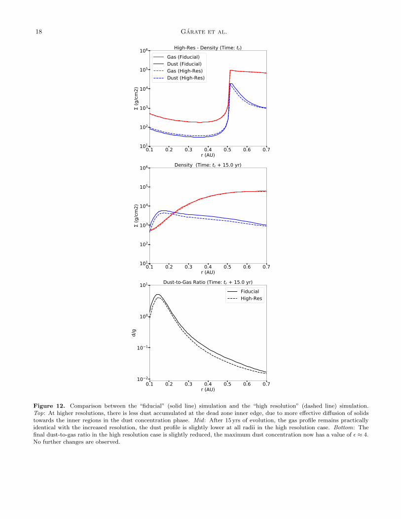
In Figure 12 we see that the evolution of gas remains the same independent of the resolution used. The final dust

surface density profile and the dust-to-gas ratio are slightly lower for the higher resolution simulation over the entire

inner region, the maximum concentration is reduced from ε = 5 to ε = 4.

This decrease in the dust surface density apparently happens because, during the dust concentration phase, the

material accumulated at the dead zone inner edge diffuses more efficiently towards the inner disk, slightly lowering

the dust-to-gas ratio in the dust trap. In the high resolution case, the accumulated dust mass between 0.51-0.6 au is

75 M⊕ (in contrast with the 110 M⊕ accumulated in the low resolution case).

Other than the slight redistribution of dust, the high resolution simulation behaves in the same way as the standard

case, and our conclusions are maintained.

We tested that the dust distribution obtained during the dust concentration phase (Phase 1) converges for resolutions

resolutions higher than nr = 1000 (tested up to nr = 3000), and therefore we do not expect any further changes in

the subsequent results after the dead zone reactivation (other than those already reported in this section).

18 Garate et al.

0.1 0.2 0.3 0.4 0.5 0.6 0.7r (AU)

101

102

103

104

105

106

(g/c

m2)

High-Res - Density (Time: tr)Gas (Fiducial)Dust (Fiducial)Gas (High-Res)Dust (High-Res)

0.1 0.2 0.3 0.4 0.5 0.6 0.7r (AU)

101

102

103

104

105

106

(g/c

m2)

Density (Time: tr + 15.0 yr)

0.1 0.2 0.3 0.4 0.5 0.6 0.7r (AU)

10 2

10 1

100

101

d/g

Dust-to-Gas Ratio (Time: tr + 15.0 yr)FiducialHigh-Res

Figure 12. Comparison between the “fiducial” (solid line) simulation and the “high resolution” (dashed line) simulation.Top: At higher resolutions, there is less dust accumulated at the dead zone inner edge, due to more effective diffusion of solidstowards the inner regions in the dust concentration phase. Mid : After 15 yrs of evolution, the gas profile remains practicallyidentical with the increased resolution, the dust profile is slightly lower at all radii in the high resolution case. Bottom: Thefinal dust-to-gas ratio in the high resolution case is slightly reduced, the maximum dust concentration now has a value of ε ≈ 4.No further changes are observed.

Dust accretion preceding an outburst? 19

REFERENCES

Akeson, R. L., Boden, A. F., Monnier, J. D., et al. 2005,

ApJ, 635, 1173

Andrews, S. M., & Williams, J. P. 2005, ApJ, 631, 1134

Antipin, S., Belinski, A., Cherepashchuk, A., et al. 2015,

Information Bulletin on Variable Stars, 6126, 1

Audard, M., Abraham, P., Dunham, M. M., et al. 2014,

Protostars and Planets VI, 387

Balbus, S. A., & Hawley, J. F. 1991, ApJ, 376, 214

Berdnikov, L. N., Burlak, M. A., Vozyakova, O. V., et al.

2017, Astrophysical Bulletin, 72, 277

Birnstiel, T., Dullemond, C. P., & Brauer, F. 2010, A&A,

513, A79

Birnstiel, T., Klahr, H., & Ercolano, B. 2012, A&A, 539,

A148

Bozhinova, I., Scholz, A., Costigan, G., et al. 2016,

MNRAS, 463, 4459

Brauer, F., Dullemond, C. P., & Henning, T. 2008, A&A,

480, 859

Cabrit, S., Pety, J., Pesenti, N., & Dougados, C. 2006,

A&A, 452, 897

Carrera, D., Gorti, U., Johansen, A., & Davies, M. B. 2017,

ApJ, 839, 16

Dipierro, G., Laibe, G., Alexander, R., & Hutchison, M.

2018, MNRAS, 479, 4187

Eisner, J. A., Hillenbrand, L. A., White, R. J., et al. 2007,

ApJ, 669, 1072

Facchini, S., Manara, C. F., Schneider, P. C., et al. 2016,

A&A, 596, A38

Gammie, C. F. 1996, ApJ, 457, 355

Garaud, P. 2007, ApJ, 671, 2091

Ghez, A. M., White, R. J., & Simon, M. 1997, ApJ, 490,

353

Gunther, H. M., Birnstiel, T., Huenemoerder, D. P., et al.

2018, AJ, 156, 56

Guttler, C., Blum, J., Zsom, A., Ormel, C. W., &

Dullemond, C. P. 2010, A&A, 513, A56

Hartigan, P., Edwards, S., & Ghandour, L. 1995, ApJ, 452,

736

Ingleby, L., Calvet, N., Herczeg, G., et al. 2013, ApJ, 767,

112

Kanagawa, K. D., Ueda, T., Muto, T., & Okuzumi, S. 2017,

ApJ, 844, 142

Kretke, K. A., Lin, D. N. C., Garaud, P., & Turner, N. J.

2009, ApJ, 690, 407

Lamzin, S., Cheryasov, D., Chuntonov, G., et al. 2017, in

Stars: From Collapse to Collapse, Vol. 510, 356

Lynden-Bell, D., & Pringle, J. E. 1974, MNRAS, 168, 603

Martin, R. G., & Lubow, S. H. 2011, ApJL, 740, L6

Nakagawa, Y., Sekiya, M., & Hayashi, C. 1986, Icarus, 67,

375

Okuzumi, S., Tanaka, H., Kobayashi, H., & Wada, K. 2012,

ApJ, 752, 106

Onishi, I. K., & Sekiya, M. 2017, Earth, Planets, and

Space, 69, 50

Ormel, C. W., & Cuzzi, J. N. 2007, A&A, 466, 413

Osterloh, M., & Beckwith, S. V. W. 1995, ApJ, 439, 288

Petrov, P. P., Gahm, G. F., Djupvik, A. A., et al. 2015,

A&A, 577, A73

Pinilla, P., Benisty, M., & Birnstiel, T. 2012, A&A, 545,

A81

Pinilla, P., Flock, M., Ovelar, M. d. J., & Birnstiel, T.

2016, A&A, 596, A81

Rodriguez, J. E., Pepper, J., Stassun, K. G., et al. 2013,

AJ, 146, 112

Rodriguez, J. E., Reed, P. A., Siverd, R. J., et al. 2016, AJ,

151, 29

Rodriguez, J. E., Loomis, R., Cabrit, S., et al. 2018, ApJ,

859, 150

Rosotti, G. P., Clarke, C. J., Manara, C. F., & Facchini, S.

2017, MNRAS, 468, 1631

Schneider, P. C., Manara, C. F., Facchini, S., et al. 2018,

A&A, 614, A108

Schneider, P. C., Gunther, H. M., Robrade, J., et al. 2015,

A&A, 584, L9

Shakura, N. I., & Sunyaev, R. A. 1973, A&A, 24, 337

Shenavrin, V. I., Petrov, P. P., & Grankin, K. N. 2015,

Information Bulletin on Variable Stars, 6143

Takeuchi, T., & Lin, D. N. C. 2002, ApJ, 581, 1344

Taki, T., Fujimoto, M., & Ida, S. 2016, A&A, 591, A86

Tanaka, H., Himeno, Y., & Ida, S. 2005, ApJ, 625, 414

Toomre, A. 1964, ApJ, 139, 1217

Weidenschilling, S. J. 1977, MNRAS, 180, 57

Whipple, F. L. 1972, in From Plasma to Planet, ed.

A. Elvius, 211

Woitas, J., Leinert, C., & Kohler, R. 2001, A&A, 376, 982

Wunsch, R., Klahr, H., & Rozyczka, M. 2005, MNRAS,

362, 361

Youdin, A. N., & Goodman, J. 2005, ApJ, 620, 459

Youdin, A. N., & Lithwick, Y. 2007, Icarus, 192, 588