the discrete fourier transform and some of its
TRANSCRIPT

The Discrete Fourier Transform
and Some of its Applications on
Image Processing
Nuria Sanchez Font
Adviser: F. Javier Soria de Diego
Master in Advanced MathematicsUniversity of BarcelonaBarcelona, January 2019


Contents
1 Introduction 1
2 Discrete Fourier Transform 52.1 Fundamentals of the Discrete Fourier Transform . . . . . . . . . . . . 52.2 The Discrete Fourier Transform as a change of basis . . . . . . . . . . 162.3 Fourier coefficients and frequencies . . . . . . . . . . . . . . . . . . . 18
3 Fast Fourier Transform 213.1 The Fast Fourier Transform algorithm . . . . . . . . . . . . . . . . . 223.2 Vector of size a power of 2 . . . . . . . . . . . . . . . . . . . . . . . . 253.3 Vector of even size but not a power of 2 . . . . . . . . . . . . . . . . . 263.4 Padding of an even sized vector . . . . . . . . . . . . . . . . . . . . . 30
4 Extension of the Fast Fourier Transform 414.1 Extension of the Fast Fourier Transform algorithm . . . . . . . . . . 414.2 Vector of odd size but not prime (extended algorithm) . . . . . . . . 444.3 Vector of even size but not a power of 2 (mixed algorithm) . . . . . . 464.4 Padding . . . . . . . . . . . . . . . . . . . . . . . . . . . . . . . . . . 48
4.4.1 Vector of prime size . . . . . . . . . . . . . . . . . . . . . . . . 484.4.2 Vector of odd size but not prime . . . . . . . . . . . . . . . . . 484.4.3 Vector of even size but not a power of two . . . . . . . . . . . 49
4.5 General procedure to compute the Fourier Transform (summary) . . . 52
5 Digital image processing 575.1 Introduction to image processing . . . . . . . . . . . . . . . . . . . . 575.2 Filtering . . . . . . . . . . . . . . . . . . . . . . . . . . . . . . . . . . 585.3 Edge detection . . . . . . . . . . . . . . . . . . . . . . . . . . . . . . 645.4 Periodic noise reduction . . . . . . . . . . . . . . . . . . . . . . . . . 675.5 Blur reduction . . . . . . . . . . . . . . . . . . . . . . . . . . . . . . . 735.6 Image reconstruction . . . . . . . . . . . . . . . . . . . . . . . . . . . 77
Appendix 85
Bibliography 91
i


Chapter 1
Introduction
The digital image processing is a field devoted to the enhancement of a given imagein order to make it more suitable for a specific purpose as well as extracting someof its particular attributes. Its applications cover a wide range of different areas:from easing visualisation of a certain body feature (by sharpening, reducing noise,improving contrast, ...) for medical recognition to edge detection so as to localisea predetermined shape and, therefore, identifying a particular element such a carplate. However, the processing may be very time consuming, which is an importantdrawback. Thus, the main challenge that digital image processing faces is the de-velopment of strategies that result in an accurate outcome while speeding up thewhole process. One of the tools introduced so as to achieve such purposes is theDiscrete Fourier Transform.
The aim of this project is to develop the Discrete Fourier Transform (DFT) inorder to see some of its applications on image processing. As we are going to discussin detail throughout the project, the role played by the DFT is the following. Thespace we are going to deal with is `2(Z/M × Z/N) (defined in Chapter 2) since, aswe are going to see in Chapter 5, a digital image is regarded as an element of suchspace. Moreover, we will focus on that type of image processing that consists inapplying a linear and translation-invariant transformation to the given picture. Aswe will develop in Section 5.2, such processing is equivalent to perform a convolutionbetween the image and some other element of `2(Z/M ×Z/N) (filtering). Since Mand N can be very large (even millions), performing convolution appears to be notonly too expensive computationally, but even unfeasible if M and N are too large.And here is where the DFT comes to play. One of its key properties is the fact thatit can turn a convolution into the Inverse Discrete Fourier Transform (IDFT) of acomponent-wise product between the DFT of two matrices (Proposition 2.1.13). Inother words, f ∗ g = (f . ∗ g)∨, where f, g ∈ `2(Z/M × Z/N) and ∗ and .∗ standsfor convolution and component-wise product respectively. But, if it is true that acomponent-wise product is, by far, less time consuming, the computation of the DFTand IDFT requires much more time, since they have to be calculated by means of achange-of-basis matrix (Section 2.2). However, as we will see, such computations canbe speeded up by implementing the Fast Fourier Transform (FFT) algorithm. Thus,
1

2
on the one hand, the introduction of the DFT leads to a faster way of processingan image. In addition, as we will see in Chapter 2, the DFT is a change of basisfrom the Euclidean to the Fourier basis, which as discussed in Section 2.3, allows afrequency analysis of the signal. Hence, on the other hand, the DFT splits a signalinto its frequency components providing key information of such signal, as illustratedin Sections 5.4 and 5.5. Therefore, the project has two main goals: studying thefiltering process and developing some examples of image processing (Chapter 5) aswell as analysing the reduction entailed by the implementation of the FFT algorithm(Chapters 3 and 4). In order to do so, it is going to be fundamental the developmentof the main properties of the DFT (Chapter 2).
Let us now describe in more detail how the project is structured. Chapter 2,which is an extension to two dimensions of [2], gathers all the essential resultsconcerning the DFT. It begins by setting the required tools to define the DiscreteFourier Transform along with its main properties (Section 2.1) whereas Sections 2.2and 2.3 are more focused on its features as a change of basis. On the one hand, theformer provides the change-of-basis matrix (which is going to be fundamental whenanalysing the computational advantage of the FFT) while, on the other hand, thelatter explains the frequency information encoded in the new coefficients. As wewill see, the new basis (Fourier basis) splits a signal into its frequency componentsin such a way that the coefficients reveal the strength of each component requiredin making up the signal. This is very useful when recovering a signal, as Section 5.4will illustrate.
In Section 3.1 we introduce the Fast Fourier Transform algorithm following theapproaches set in [2] and [8]. Since this algorithm halves a vector iteratively, themost favourable situation is that in which it is applied to a vector whose size isa power of two. That is the reason why, as also mentioned at the beginning ofChapter 3, in most of the references the FFT is only applied to vectors of such length.However, since we are interested in the computational advantage that results fromthe use of this algorithm, not only have we studied its implementation in such vectors(Section 3.2) but to any other vector of even length (Section 3.3). In both cases weprovide the number of operations required by the algorithm in order to compare itwith the ones needed by the change-of-basis matrix. Recall that in Section 2.2 weconstructed that matrix and, therefore, we know how many operations are carriedout when multiplying the matrix by the vector. By comparing such numbers we aregoing to obtain the reduction entailed by the use of the FFT. As we will see, suchreduction is greater when the vector has length a power of two which leads us to studythe padding (Section 3.4). In that section we obtain an upper bound for the errorcaused when padding a vector of any size, not necessarily even, (Proposition 3.4.3)which leads to a uniform bound for normalised vectors (Corollary 3.4.5). Finally, weparticularise the study of the padding to vectors of even size but not a power of twoin order to stablish under which hypothesis it is worth to pad a vector, that is, underwhich hypothesis the operations required for computing the FFT is smaller for thepadded vector. Moreover, we find out the reduction that ensues from padding.
Keeping in mind the fact that the FFT can only be applied to vectors of even

3 Chapter 1. Introduction
size, we begin Chapter 4 by stating the result in which this algorithm is based [2,Proposition 4.1.1]. Then, we use this result to extend the FFT to a vector of oddbut non-prime size, which we call extended algorithm (Section 4.2). In addition, thisextension allows us to introduce the mixed algorithm (Section 4.3), which improvesthe FFT algorithm for vectors of even size but not a power of two. In both cases,we compute the number of operations required by the new algorithms and compareit with the change-of-basis matrix in order to analyse the reduction. Next, in Sec-tions 4.4.2 and 4.4.3 we compare the number of operations required by the extendedor mixed algorithm with the ones needed by the FFT applied to the padded vectorso as to find out the reduction. Moreover, we study, in each case, the conditionsunder which padding is worth doing. Finally, we focus on vectors of prime size,whose only way of computing its transform is by means of the change-of-basis ma-trix. In Section 4.4.1, we examine how many operations are needed when paddingit and, as we will see, the conclusion is that padding such vectors is always lesstime-consuming.
Notice that in this two chapters we have distinguished different situations de-pending on the size of the vector discussing, in each case, the quickest way of com-puting its Fourier Transform (algorithms/padding). Section 4.5 summarises it andprovides the plots depicting the number of operations required by each algorithm(Figure 4.6) and by the FFT applied to the padded vectors (Figure 4.7), both de-pending on the length of the vectors.
Recall that we mentioned the fact that most of the references in the FFT are onlyconcerned with vectors whose size is a power of two since, otherwise, the vectors arejust padded. Therefore, the main purpose of Chapters 3 and 4 is to go deeper onthose aspects usually skipped in most of the discussions: the extension of the FFTso as to be applied to a vector of any size, the study of the reduction that ensuesfrom the implementation of the algorithms (which involves counting the numberof operations required) and a deeper discussion on the padding issue. The latterincludes bounding its error, finding the hypothesis under which it is actually time-saving and, finally, studying the consequent reduction.
Eventually, Chapter 5 focuses on digital image processing. Once it has estab-lished the setting and introduced the notation (Section 5.1) it then exposes thebasics of filtering, where the results exposed are an extension to two dimensions ofthe ones appearing in [2]. Moreover, it shows the computational reduction arisenfrom the use of the DFT instead of the convolution. Finally, this section ends withan introduction to Sections 5.3, 5.4 and 5.5, since some previous assumptions mustbe made. Such sections provide examples of digital image processing that illustratethe important role played by the Fourier Transform when filtering [3]. In addition,Section 5.4 shows how to take advantage of the information encoded in the Fourierbasis in order to eliminate periodic noise from a picture. Finally, Section 5.6 devel-ops an algorithm that can be used so as to reconstruct an image where a uniformlydistributed set of its pixels has been removed [1]. Although it is usually used withother types of transformations (such the Discrete Cosine Transform as illustratedin [1] and [7]), we are going to implement it with the DFT and see its performance

4
when a whole square of pixels is missing. Along this chapter we are going to illus-trate the approaches set with some particular examples, which were implementedusing Matlab. The codes can be found in the Appendix.

Chapter 2
Discrete Fourier Transform
In this chapter we are going to set a certain Hilbert space over which we will definea linear transformation, the Discrete Fourier Transform, which will be regarded asthe change of coordinates from the Euclidean basis to the so called Fourier basis.By extending to two dimensions the results exposed in [2], we are going to see someof its properties such as the fact that it is invertible or its performance over othertransformations like are translation or convolution. In particular, we are going topay special attention to the construction of the change-of-basis matrix. Finally, wewill see how the Fourier basis allows a frequency analysis of the vectors, fact that isgoing to be fundamental later on.
2.1 Fundamentals of the Discrete Fourier Trans-
form
In this section we are going to define the so called Discrete Fourier Transform overa certain space of functions as well as developing its main properties.
Let us first consider the set
`2 (Z/(M)× Z/(N)) = f : Z× Z→ C such that f(m,n) = f(m+ k1M,n+ k2N)
for all k1, k2 ∈ Z,
where M and N are positive integers. That is the set of discrete functions oftwo integer variables taking values in the set of complex numbers such that theyhave period M with respect to the first variable and period N with respect to thesecond variable. Notice that it is enough to have these functions defined in the set0, 1, . . . ,M − 1× 0, 1, . . . , N − 1 since, then, they can be extended periodically.Thus, any function f ∈ `2 (Z/(M)× Z/(N)) can be represented by the finite matrix
f =
f(0, 0) . . . f(0, N − 1)...
...f(M − 1, 0) . . . f(M − 1, N − 1)
. (2.1.1)
5

2.1. Fundamentals of the Discrete Fourier Transform 6
In order to simplify notation, we are going to denote ZM := Z/(M) for anyinteger M .
The set `2(ZM × ZN) is a vector space over C with the usual componentwiseaddition and scalar multiplication. Moreover, with the following inner product
〈f, g〉 =M−1∑m=0
N−1∑n=0
f(m,n)g(m,n), ∀f, g ∈ `2(ZM × ZN)
it becomes a Hilbert space. Therefore, it is a Banach space with the norm
||f || = 〈f, f〉1/2 =
(M−1∑m=0
N−1∑n=0
|f(m,n)|2)1/2
.
The standard basis for `2(ZM × ZN) is the Euclidean one, defined as E =Ep,q0≤p≤M−1,0≤q≤N−1, where
Ep,q(m,n) =
1, if m = p and n = q
0, otherwise,
for all m ∈ 0, . . . ,M − 1, n ∈ 0, . . . , N − 1 and, then, extended periodically.
Apart from this one, there is another basis that is going to be fundamental forour purposes and is the so called Fourier basis. Let us now define it.
Proposition 2.1.1. Consider the subset F = Fp,q0≤p≤M−1,0≤q≤N−1 ⊂ `2(ZM×ZN)with
Fp,q(m,n) =1√MN
e2πipm/Me2πiqn/N
for all m,n ∈ Z. Then, the set F is an orthonormal basis of the space `2(ZM ×ZN).We will refer to the set F as the Fourier basis of the space `2(ZM × ZN).
Proof. Let us first check that F is certainly contained in `2(ZM × ZN). If we takek1, k2 ∈ Z, then
Fp,q(m+ k1M,n+ k2N) =1√MN
e2πip(m+k1M)/Me2πiq(n+k2N)/N
=1√MN
e2πipm/Me2πipk1e2πiqn/Ne2πiqk2
=1√MN
e2πipm/Me2πiqn/N = Fp,q(m,n).
So the functions of F are M -periodic with respect to the first variable and N -periodicwith respect to the second variable, as we wanted to prove.

7 Chapter 2. Discrete Fourier Transform
Let us now see that the set F is orthonormal. Take 0 ≤ p1, p2 ≤ M − 1 and0 ≤ q1, q2 ≤ N − 1. Then,
〈Fp1,q1 , Fp2,q2〉 =M−1∑m=0
N−1∑n=0
Fp1,q1(m,n)Fp2,q2(m,n)
=1
MN
M−1∑m=0
N−1∑n=0
e2πip1m/Me2πiq1n/Ne−2πip2m/Me−2πiq2n/N
=1
MN
M−1∑m=0
N−1∑n=0
e2πi(p1−p2)m/Me2πi(q1−q2)n/N
=1
MN
M−1∑m=0
N−1∑n=0
(e2πi(p1−p2)/M
)m (e2πi(q1−q2)/N
)n=
1
MN
[M−1∑m=0
(e2πi(p1−p2)/M
)m][N−1∑n=0
(e2πi(q1−q2)/N
)n].
At this point we will distinguish two cases depending on the values of p1, p2, q1 andq2:
(i) If p1 = p2 and q1 = q2, then
〈Fp1,q1 , Fp1,q1〉 =1
MN
(M−1∑m=0
1
)(N−1∑n=0
1
)= 1.
(ii) Suppose now that p1 6= p2 or q1 6= q2. Without loss of generality, assumep1 6= p2. Since 0 ≤ p1, p2 ≤ M − 1, then −M + 1 ≤ p1 − p2 ≤ M − 1 and hencee2πi(p1−p2)/M 6= 1. Therefore, the sum is a geometric series, so
M−1∑m=0
(e2πi(p1−p2)/M
)m=
1− (e2πi(p1−p2)/M)M
1− e2πi(p1−p2)/M=
1− e2πi(p1−p2)
1− e2πi(p1−p2)/M
=1− 1
1− e2πi(p1−p2)/M= 0,
where we have used the fact that p1 − p2 ∈ Z. This implies that 〈Fp1,q1 , Fp2,q2〉 = 0.This proves that the set F is orthonormal. In particular, the elements of F are
linearly independent. This result together with the fact that the space `2(ZM ×ZN)has dimension M ·N implies that F generates all the space `2(ZM × ZN). So, F isan orthonormal basis of `2(ZM × ZN).
Remark 2.1.2. An important feature of this basis is the fact that
Fp,q(m,n) = Fm,n(p, q)
for all 0 ≤ m, p ≤M − 1 and 0 ≤ n, q ≤ N − 1.

2.1. Fundamentals of the Discrete Fourier Transform 8
So far we have seen that `2(ZM × ZN) is a Hilbert space with an orthonormalbasis called the Fourier basis. So we can now define the Fourier coefficients of theelements of the space.
Definition 2.1.3. We define the Discrete Fourier Transform (DFT) as the map
`2(ZM × ZN)∧−→ `2(ZM × ZN)
f 7→ f
where f(p, q) = 〈f, Fp,q〉 for all p ∈ 0, . . . ,M − 1, q ∈ 0, . . . , N − 1 and thenextended periodically.
Notice that, due to the periodicity of the Fourier basis, this definition holds forall p, q ∈ Z. Therefore, if f ∈ `2(ZM × ZN) and p, q ∈ Z, then
f(p, q) =1√MN
M−1∑m=0
N−1∑n=0
f(m,n)e−2πipm/Me−2πiqn/N . (2.1.2)
Observe that |f(p, q)| is the length of the projection of f onto the vector Fp,q ofthe basis.
Remark 2.1.4. In particular, if f ∈ `2(ZM), which means taking N = 1, then, forall p ∈ Z
f(p) =1√M
M−1∑m=0
f(m)e−2πipm/M .
Proposition 2.1.5. Let f, g ∈ `2(ZM × ZN). Then, the following identities hold:
(i) 〈f, g〉 = 〈f , g〉.
(ii) ||f || = ||f ||. This is the so called Parseval’s identity.
Proof.
(i) 〈f , g〉 =M−1∑p=0
N−1∑q=0
f(p, q)g(p, q)
=M−1∑p=0
N−1∑q=0
(M−1∑m=0
N−1∑n=0
f(m,n)Fp,q(m,n)
)M−1∑m=0
N−1∑n=0
g(m,n)Fp,q(m,n)
=
M−1∑p=0
N−1∑q=0
(M−1∑m=0
N−1∑n=0
f(m,n)Fp,q(m,n)
)(M−1∑m=0
N−1∑n=0
g(m,n)Fp,q(m,n)
)
=M−1∑p=0
N−1∑q=0
(M−1∑m=0
N−1∑n=0
M−1∑r=0
N−1∑s=0
f(m,n)Fp,q(m,n)g(r, s)Fp,q(r, s)
)
=M−1∑p=0
N−1∑q=0
M−1∑m=0
N−1∑n=0
M−1∑r=0
N−1∑s=0
f(m,n)g(r, s)Fm,n(p, q)Fr,s(p, q)

9 Chapter 2. Discrete Fourier Transform
=M−1∑m=0
N−1∑n=0
M−1∑r=0
N−1∑s=0
f(m,n)g(r, s)
(M−1∑p=0
N−1∑q=0
Fm,n(p, q)Fr,s(p, q)
)
=M−1∑m=0
N−1∑n=0
M−1∑r=0
N−1∑s=0
f(m,n)g(r, s)〈Fm,n, Fr,s〉
=M−1∑m=0
N−1∑n=0
f(m,n)g(m,n) = 〈f, g〉,
where we have used Remark 2.1.2.(ii) ||f ||2 = 〈f, f〉 = 〈f , f〉 = ||f ||2, where we have used (i).
Notice that, trivially, Parseval’s identity implies that the Discrete Fourier Trans-form `2(ZM × ZN)
∧−→ `2(ZM × ZN) is an isometry.
Proposition 2.1.6. Let f ∈ `2(ZM × ZN). Then, f can be expressed in terms ofthe Fourier basis as follows
f =M−1∑p=0
N−1∑q=0
f(p, q)Fp,q. (2.1.3)
Proof. Let k1, k2 ∈ Z. Then,
M−1∑p=0
N−1∑q=0
f(p, q)Fp,q(k1, k2) =M−1∑p=0
N−1∑q=0
〈f, Fp,q〉Fp,q(k1, k2)
=M−1∑p=0
N−1∑q=0
(M−1∑m=0
N−1∑n=0
f(m,n)Fp,q(m,n)
)Fp,q(k1, k2)
=M−1∑p=0
N−1∑q=0
M−1∑m=0
N−1∑n=0
f(m,n)Fp,q(m,n)Fp,q(k1, k2)
=M−1∑p=0
N−1∑q=0
M−1∑m=0
N−1∑n=0
f(m,n)Fm,n(p, q)Fk1,k2(p, q)
=M−1∑m=0
N−1∑n=0
f(m,n)
(M−1∑p=0
N−1∑q=0
Fk1,k2(p, q)Fm,n(p, q)
)
=M−1∑m=0
N−1∑n=0
f(m,n)〈Fk1,k2 , Fm,n〉 = f(k1, k2).
We have used Remarks 2.1.2 and, in the last equality, the fact that the Fourier basisis orthonormal.
Proposition 2.1.7. The Discrete Fourier Transform is injective and surjective and,therefore, invertible.

2.1. Fundamentals of the Discrete Fourier Transform 10
Proof. (i) Let f, g ∈ `2(ZM × ZN) such that f(p, q) = g(p, q) for all p, q ∈ Z. Then,by equation (2.1.3),
f =M−1∑p=0
N−1∑q=0
f(p, q)Fp,q =M−1∑p=0
N−1∑q=0
g(p, q)Fp,q = g
(ii) Let H ∈ `2(ZM ×ZN). Define h =∑M−1
p=0
∑N−1q=0 H(p, q)Fp,q ∈ `2(ZM ×ZN).
By equation (2.1.3), h =∑M−1
p=0
∑N−1q=0 h(p, q)Fp,q. Since F = Fp,q0≤p≤M−1,0≤q≤N−1
is a basis, then H(p, q) = h(p, q) for all p ∈ ZM , q ∈ ZN .
So the DFT `2(ZM × ZN)∧−→ `2(ZM × ZN) is invertible. We denote the Inverse
Discrete Fourier Transform (IDFT) as `2(ZM × ZN)∨−→ `2(ZM × ZN). As we have
seen, the inverse is given by equation (2.1.3). That is, if H ∈ `2(ZM × ZN), then
H =M−1∑p=0
N−1∑q=0
H(p, q)Fp,q (2.1.4)
or componentwise
H(m,n) =1√MN
M−1∑p=0
N−1∑q=0
H(p, q)e2πipm/Me2πiqn/N , (2.1.5)
for all m,n ∈ Z.
Notice that H is certainly in `2(ZM × ZN). Let k1, k2 ∈ Z. Then,
H(m+ k1M,n+ k2N) =M−1∑p=0
N−1∑q=0
H(p, q)Fp,q(m+ k1M,n+ k2N)
=M−1∑p=0
N−1∑q=0
H(p, q)Fp,q(m,n) = H(m,n).
So if f ∈ `2(ZM × ZN), then (f)∨ = f . Although the IDFT is given by equa-tion (2.1.5), it can also be expressed in terms of the DFT as the following theoremshows.
Theorem 2.1.8 (Inversion). Let f ∈ `2(ZM ×ZN). Then,ˆf ∈ `2(ZM ×ZN) and it
satisfies that, for any p, q ∈ Z,
ˆf(p, q) = f(−p,−q).
Notice that in order to carry out the IDFT of a function, it is enough to computeits DFT and then change the sign of the components.

11 Chapter 2. Discrete Fourier Transform
Proof. We will begin by checkingˆf ∈ `2(ZM × ZN). Take k1, k2 ∈ Z. Then,
ˆf(p+ k1M, q + k2N) =
1√MN
M−1∑m=0
N−1∑n=0
f(m,n)e−2πi(p+k1M)m/Me−2πi(q+k2N)n/N
=1√MN
M−1∑m=0
N−1∑n=0
f(m,n)e−2πipm/Me−2πiqn/N =ˆf(p, q).
Let us first take p ∈ 0,−1,−2, ...,−(M −1) and q ∈ 0,−1,−2, ...,−(N −1).Then,
ˆf(p, q) =
1√MN
M−1∑m=0
N−1∑n=0
f(m,n)e−2πipm/Me−2πiqn/N
=1√MN
M−1∑m=0
N−1∑n=0
[1√MN
M−1∑r=0
N−1∑s=0
f(r, s)e−2πimrM e
−2πinsN
]e−2πipmM e
−2πiqnN
=1√MN
M−1∑r=0
N−1∑s=0
f(r, s)
[M−1∑m=0
N−1∑n=0
e−2πimr/Me−2πins/Ne−2πipm/Me−2πiqn/N
]
=M−1∑r=0
N−1∑s=0
f(r, s)
[1
M
M−1∑m=0
e−2πimr/Me−2πipm/M
][1
N
N−1∑n=0
e−2πins/Ne−2πiqn/N
]
=M−1∑r=0
N−1∑s=0
f(r, s)〈F−p, Fr〉〈F−q, Fs〉 = f(−p,−q),
where we have used the fact that
〈F−p, Fr〉 =
0, if r 6= −p1, if r = −p
〈F−q, Fs〉 =
0, if s 6= −q1, if s = −q
since Fp0≤p≤M−1 is the Fourier basis in `2(ZM). Now, if p, q ∈ Z, then there existsk1, k2 ∈ Z such that −(M − 1) ≤ p + k1M ≤ 0 and −(N − 1) ≤ q + k2N ≤ 0.
Therefore, using the periodicity of f andˆf , we get
ˆf(p, q) =
ˆf(p+ k1M, q + k2N) = f(−p− k1M,−q − k2N) = f(−p,−q),
as wished.
Let us now define the translation of a function and see how the transformbehaves over it.
Definition 2.1.9. Let f ∈ `2(ZM × ZN) and k1, k2 ∈ Z. We define the translationof f by k1 and k2 as
(Rk1,k2f)(m,n) = f(m− k1, n− k2).

2.1. Fundamentals of the Discrete Fourier Transform 12
Notice that Rk1,k2f ∈ `2(ZM × ZN) as well.
Proposition 2.1.10. Let f ∈ `2(ZM × ZN) and p, q, k1, k2 ∈ Z. Then,
(Rk1,k2f)∧(p, q) = e−2πipk1/Me−2πiqk2/N f(p, q).
Proof. Let p, q, k1, k2 ∈ Z. Then,
(Rk1,k2f)∧(p, q) =1√MN
M−1∑m=0
N−1∑n=0
(Rk1,k2f)(m,n)e−2πipm/Me−2πiqn/N
=1√MN
M−1∑m=0
N−1∑n=0
f(m− k1, n− k2)e−2πipm/Me−2πiqn/N
=1√MN
M−1−k1∑r=−k1
N−1−k2∑s=−k2
f(r, s)e−2πip(r+k1)/Me−2πiq(s+k2)/N
= e−2πipk1/Me−2πiqk2/N1√MN
M−1−k1∑r=−k1
N−1−k2∑s=−k2
f(r, s)e−2πipr/Me−2πiqs/N .
Take a, b ∈ Z such that k1 + aM ∈ 0, 1, ...,M − 1 and k2 + bN ∈ 0, 1, ..., N − 1.Then, we carry out the changes of variable u = r− aM and v = s− bM , so, we get
(Rk1,k2f)∧(p, q) = e−2πipk1
M e−2πiqk2
N1√MN
M−1−k1−aM∑u=−k1−aM
N−1−k2−bN∑v=−k2−bN
[f(u+ aM, v + bN)
× e−2πip(u+aM)/Me−2πiq(v+bN)N]
= e−2πipk1/Me−2πiqk2/N1√MN
M−1−k1−aM∑u=−k1−aM
N−1−k2−bN∑v=−k2−bN
[f(u, v)
e−2πipu/Me−2πiqv/N].
By defining ` = k1 + aM and t = k2 + bN (observe that ` ∈ 0, 1, ...,M − 1 andt ∈ 0, 1, ..., N − 1), we can rewrite the previous expression as
(Rk1,k2f)∧(p, q) = e−2πipk1/Me−2πiqk2/N1√MN
M−1−`∑u=−`
N−1−t∑v=−t
f(u, v)e−2πipu/Me−2πiqv/N︸ ︷︷ ︸A
.
(2.1.6)We are now going to compute A. Keeping in mind that u is fixed, we will distinguishtwo cases.
• If t = 0, then
A =N−1∑v=0
f(u, v)e−2πipu/Me−2πiqv/N .

13 Chapter 2. Discrete Fourier Transform
• If 1 ≤ t ≤ N − 1, then
A =−1∑v=−t
f(u, v +N)e−2πipu/Me−2πiq(v+N)/N +N−1−t∑v=0
f(u, v)e−2πipu/Me−2πiqv/N
=N−1∑c=N−t
f(u, c)e−2πipu/Me−2πiqc/N +N−t−1∑v=0
f(u, v)e−2πipu/Me−2πiqv/N
=N−1∑v=0
f(u, v)e−2πipu/Me−2πiqv/N ,
where in the second equality we have considered, in the first addend, thechange of variable c = v +N .
Therefore, for all t ∈ 0, 1, ..., N − 1,
A =N−1∑v=0
f(u, v)e−2πipu/Me−2πiqv/N .
Hence, equation (2.1.6) can be rewritten as follows
(Rk1,k2f)∧(p, q) = e−2πipk1/Me−2πiqk2/N1√MN
M−1−`∑u=−`
N−1∑v=0
f(u, v)e−2πipu/Me−2πiqv/N︸ ︷︷ ︸B
.
(2.1.7)Let us now compute B. Again, we are going to distinguish two cases.
• If ` = 0, then
B =M−1∑u=0
N−1∑v=0
f(u, v)e−2πipu/Me−2πiqv/N .
• If 1 ≤ ` ≤M − 1, then
B =−1∑u=−`
N−1∑v=0
f(u+M, v)e−2πip(u+M)
M e−2πiqvN +
M−1−`∑u=0
N−1∑v=0
f(u, v)e−2πipuM e
−2πiqvN
=M−1∑c=M−`
N−1∑v=0
f(c, v)e−2πipc/Me−2πiqv/N +M−1−`∑u=0
N−1∑v=0
f(u, v)e−2πipu/me−2πiqv/N
=M−1∑u=0
N−1∑v=0
f(u, v)e−2πipu/Me−2πiqv/N ,
where in the second equality we have considered the change of variable c = u+Min the first addend.

2.1. Fundamentals of the Discrete Fourier Transform 14
Therefore, for all ` ∈ 0, 1, ...,M − 1,
B =M−1∑u=0
N−1∑v=0
f(u, v)e−2πipu/Me−2πiqv/N .
Hence, equation (2.1.7) can be rewritten as follows
(Rk1,k2f)∧(p, q) = e−2πipk1/Me−2πiqk2/N1√MN
M−1∑u=0
N−1∑v=0
f(u, v)e−2πipu/Me−2πiqv/N
= e−2πipk1/Me−2πiqk2/N f(p, q),
which is the result that we wanted to prove.
Remark 2.1.11. Notice that when proving
M−1−k1∑r=−k1
N−1−k2∑s=−k2
f(r, s)e−2πipr/Me−2πiqs/N =M−1∑u=0
N−1∑v=0
f(u, v)e−2πipu/Me−2πiqv/N ,
we have just used the fact that, for any k1, k2 ∈ Z,
f(u+ k1M, v + k2N)e−2πip(u+k1M)/Me−2πiq(v+k2N)/N = f(u, v)e−2πipu/Me−2πiqv/N .
Therefore, for all h ∈ `2(ZM × ZN), it holds that
M−1−a∑m=−a
N−1−b∑n=−b
h(m,n) =M−1∑m=0
N−1∑n=0
h(m,n),
for any a, b ∈ Z.
As we will see in the following chapters, processing an image consists in carryingout a convolution between the image and what is called a filter. So let us nowdefine this operation between two elements of `2(ZM × ZN).
Definition 2.1.12. Let f, g ∈ `2(ZM × ZN). Then, we define the convolution as
(f ∗ g)(m,n) =1√MN
M−1∑j=0
N−1∑k=0
f(m− j, n− k)g(j, k)
for all m,n ∈ Z.
Observe that f ∗ g ∈ `2(ZM × ZN). One of the most important features of theconvolution is the following property.
Proposition 2.1.13. Let f, g ∈ `2(ZM × ZN). Then,
(f ∗ g)∧(p, q) = f(p, q)g(p, q)
for all p, q ∈ Z.

15 Chapter 2. Discrete Fourier Transform
Proof.
(f ∗ g)∧(p, q) =1√MN
M−1∑m=0
N−1∑n=0
(f ∗ g)(m,n)e−2πipm/Me−2πiqn/N
=1√MN
M−1∑m=0
N−1∑n=0
(1√MN
M−1∑j=0
N−1∑k=0
f(m− j, n− k)g(j, k)
)× e−2πipm/Me−2πiqn/N
=1
MN
M−1∑m=0
N−1∑n=0
M−1∑j=0
N−1∑k=0
f(m− j, n− k)g(j, k)e−2πip(m−j)/Me−2πipj/M
× e−2πiq(n−k)/Ne−2πiqk/N
=1
MN
M−1∑j=0
N−1∑k=0
g(j, k)e−2πipj/Me−2πiqk/N
×
(M−1∑m=0
N−1∑n=0
f(m− j, n− k)e−2πip(m−j)/Me−2πiq(n−k)/N
)
By doing the changes of variable r = m− j and s = n− k and using the periodicityof the exponentials and the function f , we obtain
1
MN
M−1∑j=0
N−1∑k=0
g(j, k)e−2πipj/Me−2πiqk/N
×
(M−1∑m=0
N−1∑n=0
f(m− j, n− k)e−2πip(m−j)/Me−2πiq(n−k)/N
)
=1
MN
M−1∑j=0
N−1∑k=0
g(j, k)e−2πipj/Me−2πiqk/N
(M−1−j∑r=−j
N−1−k∑s=−k
f(r, s)e−2πipr/Me−2πiqs/N
)
=1
MN
M−1∑j=0
N−1∑k=0
g(j, k)e−2πipj/Me−2πiqk/N
(M−1∑r=0
N−1∑s=0
f(r, s)e−2πipr/Me−2πiqs/N
)
=
(1√MN
M−1∑r=0
N−1∑s=0
f(r, s)e−2πipr/Me−2πiqs/N
)
×
(1√MN
M−1∑j=0
N−1∑k=0
g(j, k)e−2πipj/Me−2πiqk/N
)= f(p, q)g(p, q).

2.2. The Discrete Fourier Transform as a change of basis 16
2.2 The Discrete Fourier Transform as a change
of basis
The equation (2.1.3) shows that, given f ∈ `2(ZM×ZN), the coordinates of this func-tion with respect to the Fourier basis are the coefficients f(p, q)0≤p≤M−1,0≤q≤N−1.Thus, we can regard the Discrete Fourier Transform as the change of coordinatesfrom the Euclidean basis to the Fourier basis. It is clear that the Discrete FourierTransform is a linear map, so it can be represented by a matrix, which is going tobe the change of basis matrix.
Let f ∈ `2(ZM×ZN). As we have already mentioned, f is completely determinedby its values in the interval 0, . . . ,M−1×0, . . . , N−1, hence it is represented bythe matrix given in the expression (2.1.1). Consider v and v as the vectors obtainedby joining the columns of the f and f matrices respectively. That is
v =
f(0, 0)...
f(M − 1, 0)f(0, 1)
...f(M − 1, 1)
...f(0, N − 1)
...f(M − 1, N − 1)
MN×1
v =
f(0, 0)...
f(M − 1, 0)
f(0, 1)...
f(M − 1, 1)...
f(0, N − 1)...
f(M − 1, N − 1)
MN×1
(2.2.1)
So v is the vector of coordinates of f with respect to the Euclidean basis and v isthe vector of coordinates of f with respect to the Fourier basis.
Let us now compute the change of basis matrix, that is W such that
v = Wv.
By equation (2.1.2),
f(p, q) =1√MN
M−1∑m=0
N−1∑n=0
f(m,n)e−2πipm/Me−2πiqn/N
=1√MN
M−1∑m=0
N−1∑n=0
f(m,n)(e−2πi/M
)pm (e−2πi/N
)qn.
Denote, for any integer K,ωK := e−2πi/K . (2.2.2)
Then, we can rewrite the previous expression as
f(p, q) =1√MN
M−1∑m=0
N−1∑n=0
f(m,n)ωpmM ωqnN . (2.2.3)
17 Chapter 2. Discrete Fourier Transform
Notice that f(m,n) = v(nM +m) and f(p, q) = v(qM + p). Hence,
v(qM + p) =1√MN
M−1∑m=0
N−1∑n=0
v(nM +m)ωpmM ωqnN .
Therefore,
W (qM + p, nM +m) =ωpmM ωqnN√MN
, (2.2.4)
for all 0 ≤ m, p ≤M − 1 and 0 ≤ n, q ≤ N − 1. Notice that W is symmetric
W (qM + p, nM +m) =ωpmM ωqnN√MN
=ωmpM ωnqN√MN
= W (nM +m, qM + p).
This result is formalised in the following proposition.
Proposition 2.2.1. Let f ∈ `2(ZM ×ZN) and v and v be the finite vectors obtainedby joining the columns of f and f respectively in the way shown in (2.2.1). Then,
v = Wv, (2.2.5)
where W is the matrix given by equation (2.2.4). That is, the DFT is given by thematrix W .
Similarly, we can find a change of basis matrix for the IDFT as shown in thefollowing proposition.
Proposition 2.2.2. Let H ∈ `2(ZM×ZN). Consider h and h to be the finite vectorsobtained by joining the columns of H and H respectively in the way shown in (2.2.1).Then,
h = Wh, (2.2.6)
where W is the matrix given by equation (2.2.4). That is, the IDFT is given by thematrix W .
Proof. By using the expression (2.2.2) in equation (2.1.5), we obtain
H(m,n) =1√MN
M−1∑p=0
N−1∑q=0
H(p, q)wpmM wqnN .
Let h and h be the vectors obtained by joining the columns of the matrices H andH respectively. Then, H(p, q) = h(qM + p) and H(m,n) = h(nM + m). It allowsus to rewrite the previous expression in the following way
h(nM +m) =1√MN
M−1∑p=0
N−1∑q=0
h(qM + p)wpmM wqnN .
Therefore, h = Ah, where A is the matrix given by
A(nM +m, qM + p) =wpmM wqnN√MN
= W (qM + p, nM +m).
However, since W is symmetric, A(nM +m, qM + p) = W (nM +m, qM + p).

2.3. Fourier coefficients and frequencies 18
2.3 Fourier coefficients and frequencies
As seen in (2.1.3), if f ∈ `2(ZM ×ZN), then it can be expressed in the Fourier basis
f =M−1∑p=0
N−1∑q=0
f(p, q)Fp,q.
Thus the Fourier coefficient f(p, q) is the weight of the vector Fp,q used in making upf and we are now going to see that it provides a frequency analysis of the function.Recall that for all m,n ∈ Z
Fp,q(m,n) =1√MN
e2πipm/Me2πiqn/N .
We will first analyse the behaviour of the discrete function
e2πipm/M = cos(2πpm/M) + i sin(2πpm/M)
with m ∈ 0, . . . ,M − 1. Let us first consider cos(2πpm/M) as a continuousfunction of m defined in the interval [0,M ] and with p fixed. This function carriesout p full cycles of the cosine wave as m goes continuously from 0 to M . That is,the function has frequency p. Therefore, as the value of p increases, the same doesthe frequency of the cosine function. However, if m is defined in the discrete set0, 1, ...,M − 1 (as is the case in which we are interested) instead of the interval[0,M ], then p is not necessarily the frequency. Let us see this fact.
Take p < M/2 a non-negative integer and define k = M − p. Observe that k isthe symmetric element of p with respect to M/2 in the interval [0,M ]. Then,
cos(2πkm/M) = cos(2π(M − p)m/M) = cos(2πm− 2πpm/M)
= cos(−2πpm/M) = cos(2πpm/M).
This implies that although cos(2πkm/M) has higher frequency with respect tocos(2πpm/M) when m ∈ [0,M ], the samples that we obtain when taking m ∈0, 1, ...,M − 1 are the same. In other words, the discrete functions cos(2πkm/M)and cos(2πpm/M) taking m ∈ 0, 1, ...,M−1 are the same and, in particular, theirfrequencies are the same, p.
As an example we can consider M = 17, p = 4 and k = M − p = 13 as shown inFigure 2.1. In this case it is clear that, although cos(2π13m/17) has higher frequencythan cos(2π4m/17) when m takes real values, they are the same function when mtakes integer values. Consequently, both functions are regarded as having period 4.
This behaviour is summarized by the fact that as p increases from 0 to theclosest integer to M/2, the discrete function cos(2πpm/M) oscillates more and morerapidly (p is the frequency). However, as p increases from [M/2] + 1 to M − 1,the discrete function cos(2πpm/M) oscillates more and more slowly (M − p is thefrequency). Therefore, higher frequencies are obtained for values of p near M/2 andlower frequencies for values of p near 0 and M − 1.

19 Chapter 2. Discrete Fourier Transform
0 2 4 6 8 10 12 14 16−1
−0.5
0
0.5
1
(a)
0 2 4 6 8 10 12 14 16−1
−0.5
0
0.5
1
(b)
Figure 2.1 (a) Overlapping of the continuous and discrete functions cos(2π4m/17)with m ∈ [0,17] and m ∈ 0, 1, ..., 16. (b) Overlapping of the continuous anddiscrete functions cos(2π13m/17) with m ∈ [0,17] and m ∈ 0, 1, ..., 16.
Let us now see that the behaviour of the sinus wave is quite the same. Take thefunction sin(2πpm/M), m ∈ 0, 1, ...,M − 1 with p < M/2 a non-negative integerand k = M − p. Then,
sin(2πkm/M) = sin(2π(M − p)m/M) = sin(2πm− 2πpm/M)
= sin(−2πpm/M) = − sin(2πpm/M).
This means that the discrete functions sin(2πpm/M) and sin(2πkm/M) have thesame frequency. So, again, if 0 ≤ p ≤ [M/2], then p is the frequency and if[M/2] < p ≤M − 1, then the frequency is M − p.
Therefore, the discrete function e2πipm/M carries out p full cycles as m goes from0 to M − 1 if 0 ≤ p ≤ [M/2]. On the other hand, it carries out M − p full cyclesas m goes from 0 to M − 1 if [M/2] < p ≤ M − 1. Thus we regard e2πipm/M as ahigh frequency vector for p near M/2 and as a low frequency vector for p near 0or M − 1. This implies that the matrix Fp,q of the Fourier basis is considered as ahigh frequency matrix if p is near M/2 and q is near N/2. On the other hand, it isconsidered a low frequency matrix if p is near 0 or M − 1 and q is near 0 or N − 1.Therefore, by the previous formula
f =M−1∑p=0
N−1∑q=0
f(p, q)Fp,q,
since |f(p, q)| is the length of the projection of f onto Fp,q, then it can be regarded asthe strength of the frequency component Fp,q needed in making up f . That is, if the
values of |f(p, q)| are high for the higher frequency components, then f has stronghigh-frequency components. On the other hand, if the values of |f(p, q)| are highfor the lower frequency components, then f has strong low-frequency components.

2.3. Fourier coefficients and frequencies 20
Observe that if we consider the expression
f =
f(0, 0) . . . f(0, N − 1)...
...
f(M − 1, 0) . . . f(M − 1, N − 1)
,
the coefficients located in the center of the matrix will correspond to higher frequen-cies, whereas the ones located near the corners will correspond to lower frequencies.
Notice that |f(p, q)| provides information about the global behaviour of f in thesense that it says whether f is made up by lower and/or higher frequency componentsbut it does not localise them.
So the modulus of the Fourier coefficients provide a frequency analysis of thefunction. On the contrary, the information encoded in its phase is not so easy tointerpret.
Let us see an example of the behaviour of the modulus of the Fourier coeffi-cients. In order to simplify visualisation we will take N = 1, so the function will beone-dimensional. Consider f(m) = sin(πm2/1024) with m ∈ 0, ..., 119. As Fig-ure 2.2 (a) shows, this function seems to have strong low-frequency components (soas to see this fact clearer we have drawn a blue line joining the points). Therefore,Figure 2.2 (b) shows that the magnitude of the higher frequency Fourier coefficients(m near 120/2) is low whereas the magnitude of the lower frequency Fourier coeffi-cients (m near 0 and 119) is high. These coefficients were computed using Matlab.
0 20 40 60 80 100−1
−0.5
0
0.5
(a)
0 20 40 60 80 100 1200
2
4
6
8
10
12
14
16
18
20
(b)
Figure 2.2 (a) f(m) = sin(πm2/1024) with m ∈ 0, ..., 119. (b) |f(m)| withm ∈ 0, ..., 119.

Chapter 3
Fast Fourier Transform
As discussed in Section 2.2, in order to compute the Discrete Fourier Transform of afunction f ∈ `2(ZM ×ZN) it is enough to multiply it by the change of basis matrix.That is
v = Wv,
where v is the vector obtained by joining the columns of f and W is the change ofbasis matrix given in the expression (2.2.4). Keeping in mind that v is an MN × 1vector and W is an MN ×MN matrix, let us analyse the computational cost ofthis change of basis. In order to do so, we are just going to take into accountmultiplications since, computationally, they require much more time than sums.
When calculating the k-th component of the vector v, v(k) =∑MN−1
n=0 W (k, n)v(n),MN multiplications are required, which implies (MN)2 for the whole vector vMN×1.Observe that these multiplications are of complex numbers and each one involvesthree different real multiplications since
(a+ bi)(c+ di) = ac+ adi+ bci− bd = (ac− bd+ ad− ad) + (ad+ bc+ bd− bd)i
= [(a− b)d+ (c− d)a] + [(a− b)d+ (c+ d)b]i.
So in order to compute v we need (MN)2 complex multiplications or, equivalently,3(MN)2 real ones.
The Discrete Fourier Transform is one of the fundamental tools in the area ofsignal processing and, in particular, in image processing. As we will see in thefollowing chapters, an image can be thought of as a matrix where each componentrepresents a pixel. That is, an image is regarded as an element of the set `2(ZM×ZN).It is common to deal with images that have thousands or even millions of pixels, socomputing the Discrete Fourier Transform of an image by means of the change-of-basis matrix appears to be a task that can take hours. For that reason, an algorithmcalled the Fast Fourier Transform (FFT) is introduced.
At the beginning of this chapter we are going to develop the steps of this well-known algorithm of the FFT following the approaches set in [2] and [8], which, likemost of the references on the topic, are only focused on vectors of length a power oftwo. However, in contrast with them, we are going to distinguish its performanceover such vectors and those of even length but not a power of two. In both cases,
21

3.1. The Fast Fourier Transform algorithm 22
we will detail the number of operations required as well as analysing the consequentreduction. Moreover, since the last will appear to be greater when the length is apower of two, we will then study under which conditions padding the vector speedsup the whole process, which is a question usually skipped in most of the discussionson the FFT. In doing so, it is going to be essential keeping the error under control.That is the reason why we will pay special attention on finding an upper bound forit. Therefore, the main goal of this chapter is to go deeper on those issues not usuallycovered in the references on the FFT such as its performance on arbitrary vectors ofeven length, the precise number of operations required or the setting where paddingimproves the computation as well as bounding its error.
3.1 The Fast Fourier Transform algorithm
Let f ∈ `2(ZM × ZN) and take v ∈ `2(ZMN) the vector obtained by joining thecolumns of f . Let us now develop the FFT algorithm in the computation of v.
By definition of the Discrete Fourier Transform (see Remark 2.1.4)
v(k) =1√MN
MN−1∑m=0
v(m)e−2πikmMN
for all 0 ≤ k ≤ MN − 1. Assume that MN is an integer multiple of 2. Then, wecan split the previous expression as follows
v(k) =1√MN
MN2−1∑
m=0
v(2m)e−2πik2mMN +
1√MN
MN2−1∑
m=0
v(2m+ 1)e−2πik2m+1MN
=1√MN
MN2−1∑
m=0
v(2m)e−2πik2mMN + e−2πi
kMN
1√MN
MN2−1∑
m=0
v(2m+ 1)e−2πik2mMN
=1√MN
MN2−1∑
m=0
v(2m)e−2πik m
MN2 + e−2πi
kMN
1√MN
MN2−1∑
m=0
v(2m+ 1)e−2πik m
MN2 .
Denoting
v0(k) =1√MN2
MN2−1∑
m=0
v(2m)e−2πik m
MN2
v1(k) =1√MN2
MN2−1∑
m=0
v(2m+ 1)e−2πik m
MN2 ,
we can rewrite
v(k) =1√2v0(k) + e−2πi
kMN
1√2v1(k).

23 Chapter 3. Fast Fourier Transform
Notice that v0(k) and v1(k) are the k-th Fourier coefficients of the `2(ZMN
2
)vectors
(v(0), v(2), ..., v(MN − 2)) and (v(1), v(3), ..., v(MN − 1)) respectively. Moreover,taking 0 ≤ k ≤ MN
2− 1, observe that
v
(k +
MN
2
)=
1√2v0
(k +
MN
2
)+ e−2πi
k+MN2
MN +1√2v1
(k +
MN
2
)=
1√2v0(k) + e−2πi
kMN e−πi +
1√2v1(k)
=1√2v0(k)− e−2πi
kMN
1√2v1(k),
where we have used the fact that v0 and v1 have period MN2
.Therefore, for 0 ≤ k ≤ MN
2− 1,
v(k) =1√2
[v0(k) + e−2πi
kMN v1(k)
]v
(MN
2+ k
)=
1√2
[v0(k)− e−2πi
kMN v1(k)
].
This result is summarized in the following proposition.
Proposition 3.1.1. Let v ∈ `2(ZM) and M ∈ 2Z. Split the vector v in the following
vectors of `2(ZM
2
)v0 = (v(0), v(2), v(4), ..., v(M − 2))
v1 = (v(1), v(3), v(5), ..., v(M − 1)).
Then, for all 0 ≤ k ≤ M2− 1, the Discrete Fourier Transform of v is
v(k) =1√2
[v0(k) + e−2πi
kM v1(k)
]v
(M
2+ k
)=
1√2
[v0(k)− e−2πi
kM v1(k)
],
(3.1.1)
where v0 and v1 are the Discrete Fourier Transforms of v0 and v1 respectively.
Let us now see, following the notation just introduced in Proposition 3.1.1, thecomputational advantage of this approach. To begin with, we are not going totake into account the division by
√2 since it is not as time consuming as complex
products. Then, the change-of-basis matrix needed in computing the DFT of thevectors v0 and v1 is of size M/2 ×M/2. Therefore, the computation of v0 and v1requires (M/2)2 complex multiplications each. Moreover, there are M/2 − 1 moredue to the multiplication by the exponentials (without considering k = 0). Thus itall requires
2
(M
2
)2
+M
2− 1 =
M2
2+M
2− 1

3.1. The Fast Fourier Transform algorithm 24
complex multiplications, which can be thought as M2
2for M large enough. Recall
that we needed M2 of these operations in order to compute v by means of thechange-of-basis matrix, so this approach cuts the computation time nearly in half.The main point of this procedure is the fact that the computation of the DFT of anM -vector is reduced to that of two M/2-vectors.
Then, returning to our initial function f ∈ `2(ZM × ZN) and its corresponding
vector v, this method will just perform (MN)2
2+ MN
2− 1 complex multiplications
when computing v, as long as MN ∈ 2Z.
In Proposition 3.1.1, we are just assuming M ∈ 2Z but notice that if M ∈ 4Zas well, then we can also apply the already mentioned proposition to the vectors
v0, v1 ∈ `2(ZM
2
), which results on a further reduction. That is, we can divide v0
and v1 obtaining the following elements of `2(ZM
4
)
v0
v00 = (v(0), v(4), v(8), ..., v(M − 4))
v01 = (v(2), v(6), v(10), ..., v(M − 2))
v1
v10 = (v(1), v(5), v(9), ..., v(M − 3))
v11 = (v(3), v(7), v(11), ..., v(M − 1)).
Then, for 0 ≤ k ≤ M4− 1, we get
v0(k) =1√2
[v00(k) + e−2πik/M v01(k)
], v0
(M
4+ k
)=
1√2
[v00(k)− e−2πik/M v01(k)
]v1(k) =
1√2
[v10(k) + e−2πik/M v11(k)
], v1
(M
4+ k
)=
1√2
[v10(k)− e−2πik/M v11(k)
](3.1.2)
Therefore, the number of complex multiplications required this time is 4(M/4)2 (dueto the four DFT) plus M/4−1+M/4−1 (regarding the exponentials in (3.1.2) with-out considering k = 0) plus another M/2−1 (regarding the exponentials in (3.1.1)).That is
M2
4+ 2
(M
4− 1
)+M
2− 1 ≈ M2
4for M large enough,
which is four times faster than using the change-of-basis matrix directly.So the Fast Fourier Transform algorithm consists in applying Proposition 3.1.1
repeatedly to the vectors that appear at each stage until it encounters odd sizedvectors. That is, if M = 2mp for some m, p ∈ N and p odd, then the algorithm willentail m stages. Notice that, in the last stage, there will be 2m vectors belonging to`2(Zp). Then, the Fourier Transforms of these vectors will be calculated by means ofthe change-of-basis-matrix. In the following sections, we are going to distinguish howthe Fast Fourier Transform applies when M = 2m and M = 2mp for some p ∈ N≥3odd as well as discussing the ensuing reduction in the number of operations.

25 Chapter 3. Fast Fourier Transform
3.2 Vector of size a power of 2
The algorithm of the Fast Fourier Transform that we have just developed leads us tothink that the most favourable case is when M = 2m for some m ∈ N, following thenotation introduced in Proposition 3.1.1. In this situation, the vector v ∈ `2(ZM)can be subdivided m = log2M times. Notice that at the last stage of divisionthere are M vectors all belonging to `2(Z1), so their Discrete Fourier Transformsare themselves. This implies that there is, actually, no need of computing anyFourier Transform, thus the only complex multiplications involved are the onesregarding the exponentials. Observe that, at the first stage of division (given byequation (3.1.1)), there are M
2− 1 multiplications of this type and, at the second
one (given by equation (3.1.2)), there are 2(M4− 1)
= M2− 2. Then, at the third
stage there would be 4(M8− 1)
= M2− 4. Hence, intuitively, in the k-th stage there
would be 2k−1(M2k− 1)
= M2− 2k−1. Since there are log2M stages, it seems that
there are
M
2log2M −
log2M−1∑n=0
2n
multiplications regarding exponentials along the algorithm. The following proposi-tion formalises this idea giving us the number of operations required.
Proposition 3.2.1. Let M = 2m for some m ∈ N. Denote as #FFTM the maximum
number of complex multiplications required to compute the Discrete Fourier Trans-form of a vector of length M by means of the Fast Fourier Transform algorithm.Then,
#FFTM =
1
2M log2M −
log2M−1∑n=0
2n = M
(log2M
2− 1
)+ 1.
Proof. We begin by proving the second equality.
1
2M log2M −
log2M−1∑n=0
2n =M
2log2M −
1− 2log2M
1− 2=M
2log2M + 1− 2log2M
=M
2log2M + 1−M = M
(log2M
2− 1
)+ 1.
We are now going to prove #FFTM = M
(log2M
2− 1)
+ 1 using induction on m.
Let v ∈ `2(ZM). If m = 1, notice that v = (v0, v1). Then, v = 1√2(v0+v1, v0−v1).
Since we don’t need any complex multiplication, #FFT2 = 0. On the other hand,
M
(log2M
2− 1
)+ 1 = 2
(1
2− 1
)+ 1 = 0.
Therefore, the equality holds when m = 1.

3.3. Vector of even size but not a power of 2 26
Assume the result true for m = k − 1. Let us now see that it also holds form = k. By Proposition 3.1.1, it is clear that
#FFTM = 2#FFT
M2
+M
2− 1 = 2#FFT
2k−1 + 2k−1 − 1.
Take M = 2k. Then,
#FFTM = #FFT
2k = 2#FFT2k−1 + 2k−1 − 1 = 2
(2k−1
(k − 1
2− 1
)+ 1
)+ 2k−1 − 1
= 2k(k − 1
2− 1
)+ 2 + 2k−1 − 1 = 2k
k
2− 2k−1 − 2k + 2k−1 + 1
= 2kk
2− 2k + 1 = 2k
(k
2− 1
)+ 1 = M
(log2M
2− 1
)+ 1,
where in the third equality we have used the hypothesis of induction.
Let us now see the reduction that ensues from the use of the Fast Fourier Trans-form instead of the change-of-basis matrix. Keeping in mind that the latter requiresM2 operations, then
M2
#FFTM
=M2
M(
log2M2− 1)
+ 1=
Mlog2M
2− 1 + 1
M
=2m
m2− 1 + 1
2m
=2m+1
m− 2 + 12m−1
≈ 2m+1
m− 2for M big enough.
This means that the computation of v ∈ `2(Z2m) by means of the FFT is 2m+1
m−2 timesfaster than using the change-of-basis matrix. The behaviour of this reduction isdepicted in Figure 3.1 (a). As an example, take a vector of size 218. Then, theFast Fourier Transform will need 218 · 8 + 1 = 2 097 153 complex multiplicationsin contrast with the (218)2 = 68 719 476 736 required by using the change-of-basismatrix. Therefore, the computation becomes more than 32 000 times faster. InFigure 3.1 (b), we can see a comparison of the number of operations required byboth methods.
3.3 Vector of even size but not a power of 2
Let us now discuss what happens if M = 2mp for some m ∈ N and p ∈ N≥3 odd,again following the notation introduced in Proposition 3.1.1. In this case, the FastFourier Transform algorithm consists on m stages where, at the last one, thereare 2m vectors belonging to `2(Zp) whose Fourier Transform must be calculated bymeans of the change-of-basis matrix. So let us now count, intuitively, the numberof operations involved. Recall that we have already discussed that, at the k-thstage of the algorithm, there are M
2− 2k−1 multiplications regarding exponentials.

27 Chapter 3. Fast Fourier Transform
4 6 8 10 12 14
1,000
2,000
3,000
4,000
5,000
m
(a)
10 20 30 40 50 60 700
1,000
2,000
3,000
4,000
M
M2
#FFTM
(b)
Figure 3.1 (a) Plot of the function 2m+1
m−2 , that is the reduction due to the use ofthe Fast Fourier Transform instead of the change-of-basis matrix. (b) Comparisonof the number of operations required by the Fast Fourier Transform and the change-of-basis matrix when M = 2m.
Therefore, it seems that the FFT requires, on the one hand, mM2−∑m−1
n=0 2n multi-plications due to exponentials and, on the other hand, 2mp2 operations regarding theFourier transforms of the last stage vectors. This idea is formalised in the followingproposition.
Proposition 3.3.1. Let v ∈ `2(ZM) with M = 2mp for some m ∈ N and p ∈ N≥3odd. Let #FFT
M be defined as in Proposition 3.2.1. Then, when computing v by meansof the Fast Fourier Transform algorithm, we have
#FFTM = m
M
2−
m−1∑n=0
2n + 2mp2 =M2
2m+M
(m
2− 1
p
)+ 1.
Proof. Let us begin by proving the second equality.
mM
2−
m−1∑n=0
2n + 2mp2 = mM
2− 1− 2m
1− 2+ 2mp2 = m
M
2+ 1− 2m + 2mp2
= mM
2+ 1− M
p+ 2m
(M
2m
)2
=M2
2m+M
(m
2− 1
p
)+ 1.
We are now going to prove #FFTM = M2
2m+M
(m2− 1
p
)+ 1 by induction on m.
If m = 1, then the vector v can be divided just once. Therefore, by Propo-sition 3.1.1, there are M
2− 1 multiplications regarding exponentials plus another
2(M2
)2= 2p2 due to the computation of v0 and v1. That is, #FFT
M = M2− 1 + 2p2.
On the other hand,
M2
2m+M
(m
2− 1
p
)+ 1 =
4p2
2+ 2p
(1
2− 1
p
)+ 1 = 2p2 + p− 2 + 1 = 2p2 +
M
2− 1.

3.3. Vector of even size but not a power of 2 28
Therefore, the equality holds for m = 1.Assume the result true for m − 1. Let us see that it also holds for m. Let
M = 2mp. By Proposition 3.1.1, it is clear that
#FFTM = 2#FFT
M2
+M
2− 1.
Then,
#FFTM = 2#FFT
M2
+M
2− 1 = 2#FFT
2m−1p +M
2− 1
= 2
(2m−1p · 2m−1p
2m−1+ 2m−1p
(m− 1
2− 1
p
)+ 1
)+
2mp
2− 1
=2mp · 2m−1p
2m−1+ 2mp
(m− 1
2− 1
p
)+ 2 +
2mp
2− 1
=2mp · 2mp
2m+ 2mp
m
2− 2mp
2− 2mp
p+
2mp
2+ 1
=M2
2m+ 2mp
(m
2− 1
p
)+ 1 =
M2
2m+M
(m
2− 1
p
)+ 1,
where in the third equality we have used the hypothesis of induction.
To get an idea of the power of this algorithm, let us now see the reduction inthe number of operations and, therefore, in computation time that the FFT entails(with respect to the change-of-basis matrix) in this case.
M2
#FFTM
=M2
M2
2m+M
(m2− 1
p
)+ 1
=M2
M(p+ m
2− 1
p
)+ 1
=M
p+ m2− 1
p+ 1
M
=2mp
p+ m2− 1
p+ 1
2mp
=2m
1 + m2p− 1
p2+ 1
2mp2
≈ 2m
1 + m2p− 1
p2
≈ 2m
1 + m2p
,
where in the first approximation we are assuming M big enough and in the secondone we are using the fact that p ≥ 3, so 1− 1
p2≈ 1.
This means that the FFT is 2m
1+m2p
times faster than using the change-of-basis
matrix. Notice that, if m is fixed, then
limp→∞
2m
1 + m2p
= 2m,
which causes the plot of the function to display a layer-like structure. This behaviouris depicted in Figure 3.2 (a) and, mostly, (b). Moreover, observe that, as opposedto the situation stated in Section 3.2, the reduction, which is not as high, is not anincreasing function.
So if p is big enough, the FFT algorithm becomes 2m times faster. In Figure 3.3,we can see a comparison of the number of operations required by both methods.Notice that we can write
#FFTM = 2mp2 + 2mp
(m
2− 1
p
)+ 1,

29 Chapter 3. Fast Fourier Transform
0 10 20 30 40 50 60 70 80 90 100
M=2mp
0
2
4
6
8
10
12
14
16
18
(a)
0 500 1000 1500 2000 2500 3000 3500 4000 4500 5000
M=2mp
0
50
100
150
200
250
300
350
400
(b)
Figure 3.2 (a) and (b) show the plots of the function 2m
1+m2p
on two different domains.
therefore, if m is fixed, then its plot is quadratic in p, as can be seen in the image.However, observe that, since the domain is M and not p, the smaller is m, the moreincreasing is #FFT
M .
0 20 40 60 80 100 120 140 160 180 200
M
0
0.5
1
1.5
2
2.5
3
3.5
4104
M2
#MFFT
Figure 3.3 Comparison of the number of operations required by the Fast FourierTransform and the change-of-basis matrix when M = 2mp.
So far, we have analysed the computational difference between the Fast FourierTransform algorithm and the calculation of the Fourier Transform through thechange-of-basis matrix distinguishing whether M = 2m or M = 2mp for some m ∈ Nand p ∈ N≥3 odd. In particular, we have seen that the latter method is always moretime-consuming. Putting together the results seen in Proposition 3.2.1 and Propo-sition 3.3.1, we can plot #FFT
M for all M ∈ N≥2 even, as Figure 3.4 shows. The bluevalues correspond to points of the type M = 2mp whereas the red ones correspond

3.4. Padding of an even sized vector 30
to points of the type M = 2m. Since the latter appear to be lower, it makes senseto set out under which circumstances it could be useful to pad the vector. This iswhat we are going to discuss next.
0 20 40 60 80 100 120 140
M
0
1000
2000
3000
4000
5000
6000
7000
8000
9000
10000
Figure 3.4 Plot of #FFTM where the blue dots are for M = 2mp and the red ones for
M = 2m.
3.4 Padding of an even sized vector
Let us begin by defining what it means to pad a vector.
Definition 3.4.1. Let v ∈ `2(ZM) with M ∈ N such that M 6= 2m for all m ∈ N. Letk ∈ N be such that 2k−1 < M < 2k. Denote as MPAD = 2k. Let vPAD ∈ `2(ZMPAD
)be defined as
vPAD(n) =
v(n), if 0 ≤ n < M
0, if M ≤ n < MPAD
.
Then, we will say that the vector vPAD is the vector v padded.
In other words, padding a vector consists in filling it with 0’s at the end until itslength becomes a power of 2.
Remark 3.4.2. Following the notation just introduced in Definition 3.4.1, let usnow find k in terms of M .
2k−1 < M < 2k ⇔ k − 1 < log2M < k,
hence k = [log2M ] + 1, where [log2 p] means the integer part of log2 p. Therefore,
MPAD = 2[log2M ]+1.

31 Chapter 3. Fast Fourier Transform
Proposition 3.4.3. Let M ∈ N such that M 6= 2m for all m ∈ N. Supposev ∈ `2(ZM). Define vPAD|M as the first M components of the Fourier Transform ofthe padded vector. Then,
||vPAD|M − v||∞ ≤ ||v||2 sup1≤n≤M−1
[M
MPAD
+ 1 +1√
M ·MPAD
× sin
(M2πn
(1
M− 1
MPAD
)) sin(
2πn(
1M− 1
MPAD
))1− cos
(2πn
(1M− 1
MPAD
))
12
.
Proof. By definition of Discrete Fourier Transform and of vPAD,
||vPAD|M − v||∞ = sup0≤n≤M−1
|vPAD(n)− v(n)|
= sup0≤n≤M−1
∣∣∣∣∣ 1√MPAD
MPAD−1∑k=0
vPAD(k)e−2πinkMPAD − 1√
M
M−1∑k=0
v(k)e−2πinkM
∣∣∣∣∣= sup
0≤n≤M−1
∣∣∣∣∣ 1√MPAD
M−1∑k=0
v(k)e−2πinkMPAD − 1√
M
M−1∑k=0
v(k)e−2πinkM
∣∣∣∣∣= sup
0≤n≤M−1
∣∣∣∣∣M−1∑k=0
v(k)
(1√
MPAD
e−2πinkMPAD − 1√
Me−2πinkM
)∣∣∣∣∣≤ sup
0≤n≤M−1
M−1∑k=0
∣∣∣∣v(k)
(1√
MPAD
e−2πinkMPAD − 1√
Me−2πinkM
)∣∣∣∣≤ sup
0≤n≤M−1||v||2
(M−1∑k=0
∣∣∣∣ 1√MPAD
e−2πinkMPAD − 1√
Me−2πinkM
∣∣∣∣2) 1
2
,
where in the last step we have used Holder’s inequality. Recall that it states that|w1w2|1 ≤ |w1|p|w2|p′ for all w1, w2 ∈ `1(Zk) and p, p′ satisfying 1
p+ 1
p′= 1. Let us
now compute the modulus.∣∣∣∣ 1√MPAD
e−2πinkMPAD − 1√
Me−2πinkM
∣∣∣∣2 =
[1√
MPAD
cos
(2πnk
MPAD
)− 1√
Mcos
(2πnk
M
)]2+
[1√M
sin
(2πnk
M
)− 1√
MPAD
sin
(2πnk
MPAD
)]2=
1
MPAD
cos2(
2πnk
MPAD
)+
1
Mcos2
(2πnk
M
)− 2
1√MPADM
cos
(2πnk
MPAD
)× cos
(2πnk
M
)+
1
MPAD
sin2
(2πnk
MPAD
)+
1
Msin2
(2πnk
M
)− 2
1√MPADM
× sin
(2πnk
MPAD
)sin
(2πnk
M
)

3.4. Padding of an even sized vector 32
=1
MPAD
+1
M− 2
1√MPADM
[cos
(2πnk
MPAD
)cos
(2πnk
M
)+ sin
(2πnk
MPAD
)sin
(2πnk
M
)]=
1
MPAD
+1
M− 2√
MPADMcos
(2πnk
MPAD
− 2πnk
M
),
where in the last equality we have used the following trigonometric identity
cos(α− β) = cos(α) cos(β) + sin(α) sin(β). (3.4.1)
Then,
||vPAD|M − v||∞ ≤
≤ ||v||2 sup0≤n≤M−1
[M−1∑k=0
(1
MPAD
+1
M− 2√
MPADMcos
(2πnk
MPAD
− 2πnk
M
))] 12
≤ ||v||2 sup0≤n≤M−1
[M
MPAD
+ 1− 2√MPADM
M−1∑k=0
cos
(2πnk
MPAD
− 2πnk
M
)] 12
= ||v||2 sup1≤n≤M−1
[M
MPAD
+ 1− 2√MPADM
M−1∑k=0
cos
(2πnk
MPAD
− 2πnk
M
)] 12
,
(3.4.2)
where the last equality is due to the fact that the cos(
2πnkMPAD
− 2πnkM
)reaches its max-
imum value when n = 0. Let us now compute the finite sum. Since cos(x) = eix+e−ix
2,
then
M−1∑k=0
cos
(2πnk
MPAD
− 2πnk
M
)=
M−1∑k=0
cos
(2πnk
M− 2πnk
MPAD
)
=1
2
M−1∑k=0
[ei2πn
(1M− 1MPAD
)]k+
1
2
M−1∑k=0
[e−i2πn
(1M− 1MPAD
)]k(3.4.3)
Keeping in mind that 1 ≤ n ≤M − 1, observe that
n
(1
M− 1
MPAD
)=n(MPAD −M)
M ·MPAD
< 1,
since nM< 1 and MPAD−M
MPAD< 1. Therefore, 0 < 2πn
(1M− 1
MPAD
)< 2π, which means
that the ratios of the geometric series appearing on equation (3.4.3) are different

33 Chapter 3. Fast Fourier Transform
from 1. Then, this equation can be expressed as follows
M−1∑k=0
cos
(2πnk
MPAD
− 2πnk
M
)=
1
2· 1− ei2πn
(1M− 1MPAD
)M
1− ei2πn(
1M− 1MPAD
) +1
2· 1− e−i2πn
(1M− 1MPAD
)M
1− e−i2πn(
1M− 1MPAD
)
=1
2· 1− e−i2πn
(1M− 1MPAD
)− ei2πn
(1M− 1MPAD
)M
+ ei2πn
(1M− 1MPAD
)(M−1)
2− ei2πn(
1M− 1MPAD
)− e−i2πn
(1M− 1MPAD
)
+1
2· 1− ei2πn
(1M− 1MPAD
)− e−i2πn
(1M− 1MPAD
)M
+ e−i2πn
(1M− 1MPAD
)(M−1)
2− ei2πn(
1M− 1MPAD
)− e−i2πn
(1M− 1MPAD
)
=1
2·
2− 2 cos(
2πn(
1M− 1
MPAD
))− 2 cos
(2πnM
(1M− 1
MPAD
))2− 2 cos
(2πn
(1M− 1
MPAD
))+
1
2·
2 cos(
2πn(M − 1)(
1M− 1
MPAD
))2− 2 cos
(2πn
(1M− 1
MPAD
))=
1
2·
1−cos(
2πn− 2πnMMPAD
)− cos
(− 2πnMMPAD
+ 2πnMPAD
+ 2πn− 2πnM
)1− cos
(2πn
(1M− 1
MPAD
))
=1
2
1−cos(
2πnMMPAD
)− cos
(2πn
(1M− 1
MPAD
)+ 2πnM
MPAD
)1− cos
(2πn
(1M− 1
MPAD
))
=1
2
1−cos(
2πnMMPAD
)− cos
(2πn
(1M− 1
MPAD
))cos(
2πnMMPAD
)1− cos
(2πn
(1M− 1
MPAD
))−
sin(
2πn(
1M− 1
MPAD
))sin(
2πnMMPAD
)1− cos
(2πn
(1M− 1
MPAD
))
=1
2
1− cos
(2πnM
MPAD
)+
sin(
2πn(
1M− 1
MPAD
))sin(
2πnMMPAD
)1− cos
(2πn
(1M− 1
MPAD
))
=1
2
1− cos
(2πnM
MPAD
)+ sin
(2πnM
MPAD
− 2πnM
M
) sin(
2πn(
1M− 1
MPAD
))1− cos
(2πn
(1M− 1
MPAD
))
=1
2
(1− cos
(2πnM
MPAD
)− sin
(M2πn
(1
M− 1
MPAD
))
×sin(
2πn(
1M− 1
MPAD
))1− cos
(2πn
(1M− 1
MPAD
)) ,
(3.4.4)

3.4. Padding of an even sized vector 34
where we have used the trigonometric identity
cos(α + β) = cos(α) cos(β)− sin(α) sin(β).
Then, we can rewrite equation (3.4.2) as follows
||vPAD − v||∞ ≤ ||v||2 sup1≤n≤M−1
[M
MPAD
+ 1− 1√MPADM
+1√
MPADMcos
(2πnM
MPAD
)+
1√MPADM
sin
(M2πn
(1
M− 1
MPAD
))
×sin(
2πn(
1M− 1
MPAD
))1− cos
(2πn
(1M− 1
MPAD
))
12
≤ ||v||2 sup1≤n≤M−1
[M
MPAD
+ 1− 1√MPADM
+1√
MPADM+
1√MPADM
× sin
(M2πn
(1
M− 1
MPAD
)) sin(
2πn(
1M− 1
MPAD
))1− cos
(2πn
(1M− 1
MPAD
))
12
= ||v||2 sup1≤n≤M−1
[M
MPAD
+ 1 +1√
MPADM
× sin
(M2πn
(1
M− 1
MPAD
)) sin(
2πn(
1M− 1
MPAD
))1− cos
(2πn
(1M− 1
MPAD
))
12
,
(3.4.5)
as we wanted to see.
Remark 3.4.4. Notice that, in expression (3.4.5), we could have finished the com-putations after the first inequality, obtaining
||vPAD − v||∞ ≤ ||v||2 sup1≤n≤M−1
[M
MPAD
+ 1− 1√MPADM
+1√
MPADMcos
(2πnM
MPAD
)+
1√MPADM
sin
(M2πn
(1
M− 1
MPAD
))
×sin(
2πn(
1M− 1
MPAD
))1− cos
(2πn
(1M− 1
MPAD
))
12
,
which is a more accurate bound than the one given in the statement. However,observe that both have the same behaviour for large values of M . Therefore, it ispreferable to work with the latter since it is more manageable.

35 Chapter 3. Fast Fourier Transform
Corollary 3.4.5. Let v ∈ `2(ZM) with M ∈ N such that M 6= 2m for all m ∈ N.Let vPAD|M be as defined in Proposition 3.4.3. Then,
||vPAD|M − v||∞ ≤√
6||v||2.
Proof. From equation (3.4.4) it follows that
−2M−1∑k=0
cos
(2πnk
MPAD
− 2πnk
M
)= −1 + cos
(2πnM
MPAD
)+ sin
(M2πn
(1
M− 1
MPAD
))
×sin(
2πn(
1M− 1
MPAD
))1− cos
(2πn
(1M− 1
MPAD
)) .(3.4.6)
Since the left term is upper bounded from above by 2M and
−2 ≤ −1 + cos
(2πnM
MPAD
)≤ 0,
then
sin
(M2πn
(1
M− 1
MPAD
)) sin(
2πn(
1M− 1
MPAD
))1− cos
(2πn
(1M− 1
MPAD
)) ≤ 2M + 2.
Therefore, using the result seen in Proposition 3.4.3,
||vPAD|M − v||∞ ≤ ||v||2 sup1≤n≤M−1
[M
MPAD
+ 1 +1√
M ·MPAD
× sin
(M2πn
(1
M− 1
MPAD
)) sin(
2πn(
1M− 1
MPAD
))1− cos
(2πn
(1M− 1
MPAD
))
12
≤ ||v||2 sup1≤n≤M−1
[M
MPAD
+ 1 +2M + 2√MPADM
] 12
= ||v||2
[M
MPAD
+ 1 + 2
√M
MPAD
+2√
MPADM
] 12
≤√
6||v||2.
Remark 3.4.6. Notice that applying the argument used in the proof of the Corol-lary 3.4.5, in particular equation (3.4.6), to the bound mentioned in Remark 3.4.4,we get
||vPAD|M − v||∞ ≤ ||v||2[
M
MPAD
+ 1 +2M√
MPADM
] 12
≤ 2||v||2,
which is a bit more accurate.

3.4. Padding of an even sized vector 36
Figure 3.5 shows a plot of the function
sup1≤n≤M−1
[M
MPAD
+ 1 +1√
M ·MPAD
sin
(M2πn
(1
M− 1
MPAD
))
×sin(
2πn(
1M− 1
MPAD
))1− cos
(2πn
(1M− 1
MPAD
))
12 (3.4.7)
for the values of M on the interval 0 < M ≤ 1 000 000. There, we can see that itactually remains below
√6 ∼ 2.45.
0 50 100 150 200 250 300 350
M
1.2
1.3
1.4
1.5
1.6
1.7
1.8
1.9
2
(a)
0 1 2 3 4 5 6 7 8 9 10
M 105
1.2
1.4
1.6
1.8
2
2.2
2.4
(b)
Figure 3.5 Plot of the function (3.4.7) in two different domains
So, provided that ||vPAD|M − v||∞ is small enough, the discussion of the Sec-tions 3.2 and 3.3 brings up the question of when it could be useful to compute vthrough vPAD. That is, instead of applying the FFT to v, applying it to vPAD andthen just keep the first M components of the latter. One situation in which it ispreferable to compute vPAD instead of v is when the number of multiplications re-quired in computing v is higher in comparison to that of vPAD. Let us now see whensuch situation occurs.
Let v ∈ `2(ZM) with M = 2mp for some m ∈ N and p ∈ N≥3 odd. Then, byPropositions 3.2.1 and 3.3.1 and Remark 3.4.2, we know that
#FFTMPAD
= MPAD
(log2MPAD
2− 1
)+ 1 =
MPAD
2log2MPAD −MPAD + 1
=2m · 21+[log2 p]
2(m+ 1 + [log2 p])− 2m · 21+[log2 p] + 1
#FFTM =
M2
2m+M
(m
2− 1
p
)+ 1 =
2m · 2mp2
2m+ 2mp
(m
2− 1
p
)+ 1
= 2mp2 +2mpm
2− 2m + 1.

37 Chapter 3. Fast Fourier Transform
We want to see when #FFTM > #FFT
MPAD. That is,
2mp2 +2mpm
2− 2m + 1 >
2m · 21+[log2 p]
2(m+ 1 + [log2 p])− 2m · 21+[log2 p] + 1
m
p2 +pm
2− 1 > 2[log2 p] (m+ 1 + [log2 p])− 21+[log2 p]
mpm
2− 2[log2 p]m > 2[log2 p] (1 + [log2 p])− 21+[log2 p] + 1− p2.
(3.4.8)
Observe that p2− 2[log2 p] < 0 since
p
2− 2[log2 p] < 0⇔ p
2< 2[log2 p] ⇔ p < 2[log2 p]+1, (3.4.9)
which is true for all p ∈ N. Therefore, #FFTM > #FFT
MPADif and only if
m <2[log2 p] (1 + [log2 p])− 21+[log2 p] + 1− p2
p2− 2[log2 p]
=2[log2 p] ([log2 p]− 1) + 1− p2
p2− 2[log2 p]
=2[log2 p]+1 ([log2 p]− 1) + 2− 2p2
p− 2[log2 p]+1.
In conclusion, #FFTM > #FFT
MPADif and only if
m <2[log2 p]+1 ([log2 p]− 1) + 2− 2p2
p− 2[log2 p]+1. (3.4.10)
So in case m satisfies inequality (3.4.10), it is faster to compute vPAD and thenkeeping the first M components than computing v. Let us now analyse the behaviourof this function.
By looking at Figure 3.6 (a) and (b), we get an idea of the performance of theexpression (3.4.10) as a function of p. However, by looking at (c), we can see thatthe larger p is, the wider the range of values of m satisfying inequality (3.4.10) is.However, we also observe that there is a certain set of points where the values ofthe function
2[log2 p]+1 ([log2 p]− 1) + 2− 2p2
p− 2[log2 p]+1
blow up. Notice that these are the points where the denominator takes lower values,that is, when p approaches 21+[log2 p] or, equivalently, when log2 p−[log2 p] approaches1. In other words, these are the values of p near the jumps of the function [log2 p],which can be seen in Figure 3.6 (d).
Going back to the inequality (3.4.10), if, for instance, M = 218 · 3, then
18 = m ≮2[log2 p]+1 ([log2 p]− 1) + 2− 2p2
p− 2[log2 p]+1= 16.

3.4. Padding of an even sized vector 38
0 5 10 15 20 25 30 35 40 45 50
p
0
200
400
600
800
1000
1200
1400
1600
1800
2000
(a)
0 100 200 300 400 500 600
p
0
1
2
3
4
5
6105
(b)
0 500 1000 1500 2000 2500 3000 3500 4000 4500 5000
p
0
0.2
0.4
0.6
0.8
1
1.2
1.4
1.6
1.8
2104
(c)
0 100 200 300 400 500 600
p
0
1
2
3
4
5
6
7
8
9
10
log2(p)
[log2(p)]
(d)
Figure 3.6 (a) and (b) show the plots of the function 2[log2 p]+1([log2 p]−1)+2−2p2p−2[log2 p]+1 on two
different domains. (c) Shows the plot of the same function than (a) and (b) althoughin a much larger domain and with its image limited to the interval [0,20000]. (d) Isa comparative of the functions log2 p and [log2 p].
Thus, in this case, we would compute v directly using the FFT rather than paddingthe vector and computing its transform. On the contrary, if M = 218 · 93, then
18 = m <2[log2 p]+1 ([log2 p]− 1) + 2− 2p2
p− 2[log2 p]+1≈ 476.
Therefore, in this situation, it would take less time computing the transform of thepadded vector, as long as ||vPAD|M − v||∞ is small enough.
Observe that
#FFTM
#FFTMPAD
=
M2
2m+M
(m2− 1
p
)+ 1
MPAD
2log2MPAD −MPAD + 1
=2mp2 + 2mp
(m2− 1
p
)+ 1
2m+[log2 p] (1 +m+ [log2 p])− 2m+1+[log2 p] + 1≈
2mp2 + 2mp(m2− 1
p
)2m+[log2 p] (−1 +m+ [log2 p]) + 1
.

39 Chapter 3. Fast Fourier Transform
Then, cancelling terms and using the fact that 2[log2 p] < p,
#FFTM
#FFTMPAD
≈p2 + p
(m2− 1
p
)2[log2 p](−1 +m+ [log2 p]) + 1
2m
>p2 + p
(m2− 1
p
)p(−1 +m+ [log2 p]) + 1
2m
=p+
(m2− 1
p
)m− 1 + [log2 p] + 1
2mp
−−−→p→∞
∞.
So if m satisfies inequality (3.4.10), then the larger p is, the faster the computationof vPAD is in comparison to v (by means of the Fast Fourier Transform). Thisbehaviour can be seen in Figure 3.7, where we have compared #FFT
M and #FFTMPAD
form = 500. In (a) we can see that if p is, approximately, less than 160, then #FFT
MPAD
is not necessarily less than #FFTM , so the vector should not be padded. However, (b)
shows that as p increases, #FFTMPAD
becomes much lower than #FFTM , so padding the
vector would save a lot of time.Putting these results together, assume that v ∈ `2(Z2mp) for some m ∈ N and
p ∈ N≥3 odd and we want to compute v. Then, if m satisfies inequality (3.4.10)and ||vPAD|M − v|| is small enough, then it is faster to compute vPAD (by meansof the FFT) and then keeping the first M components of it. On the contrary, ifone of these two conditions fails to be true, then we have to apply the Fast FourierTransform algorithm to the vector v itself.
50 100 150 200 250 300 350 400 450 500
p
0
2
4
6
8
10
12
1410155
#MFFT
#M
PAD
FFT
(a)
200 400 600 800 1000 1200 1400 1600 1800 2000
p
0
5
10
1510156
#MFFT
#M
PAD
FFT
(b)
Figure 3.7 (a) Shows a comparative of #FFTM and #FFT
MPADfor M = 2500p on a small
domain. (b) Shows the same as (a) but on a larger domain.


Chapter 4
Extension of the Fast FourierTransform
In this chapter we are going to state the result on which the FFT algorithm is based,Proposition 4.1.1, which can be found in [2]. Following this idea, we are going toextend this algorithm to another one that applies to vectors of any size, not justeven. Hence, the first concern is going to be its performance over vectors of oddlength. The results found will lead to the mixed algorithm, an improvement of theFFT for the vectors of even length but not a power of two which will arise, again, thepadding discussion. In each of these two cases mentioned, we are going to precise thenumber of operations required by the corresponding approach as well as analysingthe reduction that follows. Since we will end up with a wide range of algorithms,Section 4.5 provides a summary of the different situations that we can encounterand gives the algorithm that should be used in each of them.
4.1 Extension of the Fast Fourier Transform al-
gorithm
Let us begin by formulating the main result behind the FFT that, as mentionedabove, will allow its extension.
Proposition 4.1.1. Let v ∈ `2(ZM) and M = pq for some p, q ∈ N>1. Define thevectors x0, x1, ..., xp−1 ∈ `2(Zq) as
x`(k) = v(kp+ `) for k = 0, 1, ..., q − 1.
Then, for a = 0, 1, ..., p− 1 and b = 0, 1, ..., q − 1
v(aq + b) =1√p
p−1∑k=0
e−2πik(bM
+ap)xk(b). (4.1.1)
Notice that every m = 0, 1, ...,M − 1 can be expressed as m = aq + b for somea ∈ 0, 1, ..., p − 1 and b ∈ 0, 1, ..., q − 1, so equation (4.1.1) gives the full DFTof v.
41

4.1. Extension of the Fast Fourier Transform algorithm 42
Proof. Let 0 ≤ m ≤M − 1 and a ∈ 0, 1, ..., p− 1, b ∈ 0, 1, ..., q− 1 be such thatm = aq + b. Then,
v(m) = v(aq + b) =1√M
M−1∑k=0
v(k)e−2πi(aq+b)k/M .
Notice that there exist r ∈ 0, 1, ..., q−1 and s ∈ 0, 1, ..., p−1 such that k = rp+s.Hence,
v(aq + b) =1√M
p−1∑s=0
q−1∑r=0
v(rp+ s)e−2πi(aq+b)(rp+s)/(pq).
Since,e−2πi(aq+b)(rp+s)/(pq) = e−2πiare−2πias/pe−2πibr/qe−2πibs/(pq),
then
v(aq + b) =1√M
p−1∑s=0
e−2πias/pe−2πibs/Mq−1∑r=0
v(rp+ s)e−2πibr/q
=1√p
p−1∑s=0
e−2πias/pe−2πibs/M
(1√q
q−1∑r=0
xs(r)e−2πibr/q
)
=1√p
p−1∑s=0
e−2πias/pe−2πibs/M xs(b) =1√p
p−1∑s=0
e−2πis(ap+ bM )xs(b).
The reduction that this approach entails is based on the fact that, by equa-tion (4.1.1), for each value of a, we need to compute xk for all k. So, the algorithmthat we are now going to develop recognises this fact and calculates xk just once.
Notice that, if q is not a prime number, then we can apply again Proposition 4.1.1so as to compute x` for all 0 ≤ ` ≤ p− 1. This iteration of the procedure allows thedevelopment of the following algorithm. We are going to follow the notation justintroduced. Let M = p1p2 · · · pr for some p1, p2, ..., pr prime numbers, not necessarilydifferent, strictly greater than 1. For reasons that we are going to see afterwards, inRemark 4.2.2, let p1 ≥ p2 ≥ p3 ≥ ... ≥ pr. Now, take p = p1 and q = p2p3 · · · pr andapply Proposition 4.1.1. Then, for a = 0, 1, ..., p− 1 and b = 0, 1, ..., q − 1
v(aq + b) =1√p
p−1∑k=0
e−2πik(bM
+ap)xk(b).
In order to compute x`, take p = p2 and q = p3p4 · · · pr and, again, apply the previousresult to the vector x ∈ `2(Zp2p3···pr). Then, for c = 0, 1, ..., p−1 and d = 0, 1, ..., q−1
v(cq + d) =1√p
p−1∑k=0
e−2πik
(d
p2p3···pr+ cp
)yk(d),

43 Chapter 4. Extension of the Fast Fourier Transform
wherey`(k) = x(kp+ l) for k = 0, 1, ..., q − 1.
One more time, we implement the result to y` taking p = p3 and q = p4p5 · · · pr so asto obtain y`. And we keep applying the proposition in order to compute the FourierTransforms until a set of vectors of size pr arises. At this point we perform the laststep of the algorithm, which consists in calculating its transforms by means of thechange-of-basis matrix, since pr is prime.
Notice that, apart from the algorithm that we have just set out, Proposition 4.1.1gives rise to many others. For instance, we could take, in the first step, p = p1p2 andq = p3p4...pr. So, a wide range of different algorithms could be developed as long asthey are computationally faster than using the change-of-basis matrix, which is themain goal.
Remark 4.1.2. In the particular case of M even, Proposition 4.1.1 becomes Propo-sition 3.1.1 and, therefore, the preceding algorithm almost becomes the Fast FourierTransform. That is the reason why, from now on, we are going to refer to it as theextended algorithm. Let us now see this fact. Taking p = 2, we get the vectors
x0 = (v(0), v(2), v(4), ..., v(2q − 2)) = (v(0), v(2), v(4), ..., v(M − 2))
x1 = (v(1), v(3), v(5), ..., v(2q − 1)) = (v(1), v(3), v(5), ..., v(M − 1)).
Hence, for all 0 ≤ b ≤ M2− 1,
v(b) =1√2
1∑k=0
e−2πikb/M xk(b) =1√2
[x0(b) + e−2πib/M x1(b)
]v
(M
2+ b
)=
1√2
1∑k=0
e−2πik(bM
+ 12)xk(b) =
1√2
[x0(b) + e−2πi(
bM
+ 12)x1(b)
]=
1√2
[x0(b)− e−2πib/M x1(b)
].
Notice that, actually, the extended algorithm does not recognise the fact thatfor a = 0 and a = 1 the products by the exponentials are the same. In other words,equation (4.1.1) shows that the algorithm carries out p− 1 multiplications for eachvalue of a. This implies that, in the particular case when M is even, it is less timeconsuming applying the Fast Fourier Transform rather than the extended algorithm.So, we will only implement the latter in the case M is odd and non-prime. Observethat, in this case, it is not possible to obtain a reduction in the number of productssince such a reduction can only occur if
e−2πik(bM
+ap)xk(b) = −e−2πikb/M xk(b)
for some values of k and a, as happened when M was even and we took p = 2. IfM is odd, so must be p, which implies that 2ka/p could never be an odd integer forany values of k and a. Therefore,
e−2πik(bM
+ap)xk(b) 6= −e−2πikb/M xk(b)

4.2. Vector of odd size but not prime (extended algorithm) 44
for all possible values of k and a. So, as opposed to the case when M is even, inthis case we cannot reduce the number of multiplications by the exponential.
Since, as already mentioned, the FFT is preferable over the extended algorithmwhen M is even, let us now focus on the case when M is odd.
4.2 Vector of odd size but not prime (extended
algorithm)
In this section we are going to centre attention on how the extended algorithmperforms when computing the Fourier Transform of a vector of length M withM = p1p2 · · · pr for some p1, p2, ..., pr prime numbers strictly greater than one.Moreover, we are going to assume r ≥ 2, since if M is prime, the algorithm doesnot apply.
Let us begin by studying the number of complex multiplications required incarrying out the algorithm. First, let us count the complex products needed ineach of its steps or, equivalently, the ones appearing in Proposition 4.1.1. If wedefine, similarly as we have done in Chapter 3, #ext
M as the number of these typeof operations that arise in computing the DFT of a vector of length M using theextended algorithm, then we need, on the one hand, x` for all 0 ≤ ` ≤ p− 1, whichis p#ext
q . As we have already discussed at the end of Section 4.1, there are, on theother hand, p− 1 more products due to the multiplications by the exponentials foreach value of a. Hence, the number of operations required in Proposition 4.1.1 is
#extM = p#ext
q + p(p− 1). (4.2.1)
Recall that we are not taking into account the multiplication by 1√p
since this is not
as time consuming as a complex product. Keeping in mind the number of productsrequired at each step, we can now state the total number of them needed along thealgorithm.
Proposition 4.2.1. Let v ∈ `2(ZM) and M an odd and non-prime number. Thatis, M = p1p2 · · · pr for some pj ∈ Z≥3 prime for all 1 ≤ j ≤ r. Then, the number ofcomplex multiplications required along the extended algorithm is
#extM = M
(pr +
r−1∑k=1
pr−k − 1∏k−1j=0 pr−j
)= M
(pr +
pr−1 − 1
pr+pr−2 − 1
pr−1pr+ · · ·+ p1 − 1
p2p3...pr
).
Proof. We are going to prove it by induction on r. Let r = 2, that is M = p1p2. Inthis case we just have to apply Proposition 4.1.1 once. Then, by equation (4.2.1),
#extM = p1 #ext
p2+ p1(p1 − 1) = p1p
22 + p1(p1 − 1) = M
(p2 +
p1 − 1
p2
).

45 Chapter 4. Extension of the Fast Fourier Transform
Assume, now, the result true for r. Let us now see that it also holds for r + 1, sowe are taking M = p1p2 · · · pr+1. By equation (4.2.1),
#extM = p1 #ext
p2p3···pr+1+ p1(p1 − 1)
= p1
[p2p3 · · · pr+1
(pr+1 +
r−1∑k=1
p(r+1)−k − 1∏k−1j=0 p(r+1)−j
)]+ p1(p1 − 1)
= M
(pr+1 +
r−1∑k=1
p(r+1)−k − 1∏k−1j=0 p(r+1)−j
)+ p1(p1 − 1)
= M
(pr+1 +
r−1∑k=1
p(r+1)−k − 1∏k−1j=0 p(r+1)−j
+p1 − 1
p2p3 · · · pr
)
= M
(pr+1 +
r∑k=1
p(r+1)−k − 1∏k−1j=0 p(r+1)−j
)where in the second equality we have used the hypothesis of induction.
Remark 4.2.2. Notice that, when r = 2, the function p2 + p1−1p2
satisfies the follow-ing.
• If p1 ≈ p2, then p2 + p1−1p2≈ p1 + p2−1
p1.
• If p1 < p2, then p2 < p2 + p1−1p2
< p2 + 1. Hence, p2 + p1−1p2≈ p2.
• If p1 >> p2, then p2 + p1−1p2
< p2 + p1p2<< p1.
Therefore, taking p1 ≥ p2 ≥ ... ≥ pr seems to be a good choice for reducing thenumber of operations. That is the reason why, when the developing the algorithm,we have sorted the prime numbers as a decreasing sequence.
In order to analyse the computational advantage that this approach entails,we are going to compare the two values #ext
M and M2. We will use the fact thatp1 ≥ pj ≥ 3 for all possible values of j.
M2
#extM
=p1 · · · pr
pr + pr−1−1pr
+ pr−2−1pr−1pr
+ · · ·+ p1−1p2···pr
≥ p1 · · · prpr + pr−1
pr+ pr−2
pr−1pr+ · · ·+ p1
p2···pr
≥ p1 · · · prp1 + p1
pr+ p1
pr−1pr+ · · ·+ p1
p2···pr=
11
p2···pr + 1p2···pr−1p2r
+ 1p2···pr−2p2r−1p
2r
+ · · ·+ 1p22···p2r
≥ 1
r 1p2···pr
=p2 · · · pr
r≥ 3r−1
r≥ 3
2> 1.
The second-to-last step is due to the fact that r ≥ 2 and the function 3r−1
ris
increasing in this set of values. So, since, for all values of M , M2 > #extM , the
extended algorithm is always faster. Moreover, notice that, on the one hand,
p2 · · · prr
−−−−→pp1→∞
∞

4.3. Vector of even size but not a power of 2 (mixed algorithm) 46
and, on the other hand,p2 · · · pr
r≥ 3r−1
r−−−→r→∞
∞,
which implies that the reduction in the number of operations increases as p or rgrows, or equivalently, as M grows, as can be seen in Figure 4.1 (a). Moreover,notice that the tendency of #ext
M is
#extM ≈ p1 · · · pr−1p2r + p1 · · · pr−2p2r−1 + · · ·+ p1p
22 + p21
if the prime numbers are big enough. Therefore, fixing p2, p3, ..., pr, it is quadraticon p1, although this behaviour can only be observed when p1 is, by far, greater thanthe other primes. This fact is depicted in Figure 4.1 (b).
0 100 200 300 400 500 600 700 800 900 1000
M
0
1
2
3
4
5
6
7
8
9
10105
M2
#Mext
(a)
0 200 400 600 800 1000 1200 1400 1600 1800 2000
M
0
0.5
1
1.5
2
2.5
3
3.5
4
4.5105
(b)
Figure 4.1 (a) Comparison of the number of operations required by the extendedalgorithm and the change-of-basis matrix when M is odd and non-prime. (b) Plotof the function #ext
M when M is odd and non-prime.
Recall that we said that, for even values of M , it was faster to use the FFT thanthe extended algorithm. However, since, as we have seen, the latter is faster thanthe matrix, it seems that we could obtain an even faster algorithm for when M iseven if we mixed the FFT and the extended one. That is what we are going to studynext.
4.3 Vector of even size but not a power of 2 (mixed
algorithm)
Let us begin by recalling how the Fast Fourier Transform performed over vectors ofsize M = 2mp for some m ∈ N and p ∈ N≥3 odd.
In Section 3.3 we saw that, for such an M , the FFT consisted on m stages where,at the last one, there were 2m vectors belonging to `2(Zp) whose Fourier Transform

47 Chapter 4. Extension of the Fast Fourier Transform
must be calculated by means of the change-of-basis matrix. Then, Proposition 3.3.1showed that the number of operations required was
#FFTM = 2mp2 +M
(m
2− 1
p
)+ 1,
where M(m2− 1
p
)+ 1 was due to the product by the exponentials whereas 2mp2
resulted from the computation of the 2m Fourier Transforms of length p. However,notice that, if p is not a prime number, then the transforms can be computed bymeans of the extended algorithm, which, as we have seen in Section 4.2, is faster.Therefore, if we denote as #mix
M as the number of complex products required whenapplying this mixed algorithm, that is FFT until we get 2m vectors of length p andthen the extended algorithm for computing its transforms, then
#mixM = 2m#ext
p +M
(m
2− 1
p
)+1 = 2mp
(pr +
r−1∑k=1
pr−k − 1∏k−1j=0 pr−j
)+M
(m
2− 1
p
)+1,
(4.3.1)where we are assuming p = p1, p2 · · · , pr for p1 ≥ p2 ≥ · · · ≥ pr are prime numbersstrictly greater than 1. Notice that if p is prime, then #mix
M = #FFTM since p = pr
and the sum will have no terms.Figure 4.2 (a) shows a comparative of the functions #FFT
M and #mixM for that values
of M = 2mp where p is not a prime number. In it, we can see the significant reductionthat the mixed algorithm entails. Moreover, notice that, if we fix m, the behaviourof #mix
M is going to be determined by that of #extp , which we have already discussed
in Section 4.2. However, in comparison to the latter, the quadratic behaviour of theformer requires greater values of M to be appreciated as Figure 4.2 (b) shows.
0 50 100 150 200 250 300
M
0
0.5
1
1.5
2
2.5
3
3.5
4
4.5104
#MFFT
#Mmix
(a)
0 500 1000 1500 2000 2500 3000 3500 4000 4500 5000
M
0
2
4
6
8
10
12
14105
(b)
Figure 4.2 (a) Plot of the functions #FFTM and #mix
M at the points M = 2mp wherep is not a prime number. (b) Plot of the function #mix
M for the same points as (a).

4.4. Padding 48
4.4 Padding
So far, we have developed three different algorithms depending on the size of thevector: FFT (if it is a power of two), extended (if it is odd and non-prime) andmixed (if it is even but not a power of two). Since the first one appears to entailthe greatest reduction, we are now going to analyse whether it is worth to pad thevector so as to apply the FFT. That is on what we are going to focus now.
As discussed in Section 3.4, padding is going to be useful as long as the errorthat follows from performing the FFT of the padded vector is small enough andthe number of operations is reduced. Since Proposition 3.4.3 already gave an upperbound for the former, let us now fix our attention on the latter.
From now on, M is going to denote the length of the vector.
4.4.1 Vector of prime size
Notice that none of the algorithms developed so far apply to vectors of prime length,which means that its Fourier Transform can only be computed by means of thechange-of-basis matrix, involving M2 operations. Let us now analyse under whichconditions #FFT
MPAD< M2. Observe that we can assume M ≥ 3 since if M = 1,
the Fourier Transform is the vector itself and if M = 2, M = MPAD. Then, byRemark 3.4.2 and Proposition 3.2.1,
#FFTMPAD
= 2[log2M ]+1
(log2 2[log2M ]+1
2− 1
)+ 1 = 2[log2M ]+1
([log2M ] + 1
2− 1
)+ 1
= 2[log2M ] ([log2M ]− 1) + 1 < 2[log2M ][log2M ] < M2,
where the first inequality is due to the fact that 2[log2M ] > 1 for M ≥ 3.Therefore, if M is prime, it is always faster to compute the FFT of the padded
vector and then keep the first M components, as Figure 4.3 (a) shows (provided thatthe error is small enough). Moreover, as can be seen in Figure 4.3 (b), the reductionthat the padding entails is greater as M grows, although it is not an increasingfunction.
4.4.2 Vector of odd size but not prime
Following the notation introduced in Section 4.2, let M = p1p2...pr. In this case,the vector should be padded if #FFT
MPAD< #ext
M , that is, using the computations doneabove,
2[log2M ] ([log2M ]− 1) + 1 < M
(pr +
r−1∑k=1
pr−k − 1∏k−1j=0 pr−j
). (4.4.1)
Unlike the other cases where we have studied the implementation of the padding,we are not going to manipulate this expression in order to isolate one of its variablessince, when doing so, we get a less manageable inequality. Figure 4.4 (a) shows acomparison of these two functions. There, we can see that there are some points

49 Chapter 4. Extension of the Fast Fourier Transform
0 10 20 30 40 50 60 70 80 90 100
M
0
1000
2000
3000
4000
5000
6000
7000
8000
9000
10000
M2
#M
PAD
FFT
(a)
0 100 200 300 400 500 600 700 800 900 1000
M
0
50
100
150
200
250
(b)
Figure 4.3 (a) Comparison of the functions M2 and #FFTMPAD
over prime values of
M . (b) Plot of the function M2
#FFTMPAD
for M prime.
where padding is more time consuming, such as M = 273 or M = 297. Let us nowsee the reduction that follows from padding. Since M ≤ 2[log2M ] for M ≥ 2, then
#extM
#FFTMPAD
=
M
(pr +
∑r−1k=1
pr−k−1∏k−1j=0 pr−j
)2[log2M ] ([log2M ]− 1) + 1
≥pr +
∑r−1k=1
pr−k−1∏k−1j=0 pr−j
[log2M ]− 1 + 1M
=pr + pr−1−1
pr+ pr−2−1
pr−1pr+ · · ·+ p1−1
p2p3...pr
[log2M ]− 1 + 1M
−−−−→p1→∞
∞.
Therefore, as p1 increases so does the reduction. However, notice that this growthbecomes significant when p1 >> p2, p3, ..., pr. This behaviour is depicted in Fig-ure 4.4 (b).
4.4.3 Vector of even size but not a power of two
Following the notation introduced so far, recall that, for M = 2mp, we get
MPAD = 2m+1+[log2 p]
#FFTMPAD
= 2m+[log2 p](m+ 1 + [log2 p])− 2m+1+[log2 p] + 1
#mixM = 2mp
(pr +
r−1∑k=1
pr−k − 1∏k−1j=0 pr−j
)+ 2mp
(m
2− 1
p
)+ 1.

4.4. Padding 50
0 50 100 150 200 250 300 350 400 450 500
M
0
0.5
1
1.5
2
2.5
3104
#Mext
#M
PAD
FFT
(a)
0 500 1000 1500 2000 2500 3000 3500 4000 4500 5000
M
0
10
20
30
40
50
60
70
80
90
100
(b)
Figure 4.4 (a) Comparison of the functions #extM and #FFT
MPADover odd and non-
prime values of M . (b) Plot of the function#extM
#FFTMPAD
for M odd and non-prime.
After simplifying some terms, we see that #mixM > #FFT
MPADif and only if
p
(pr +
r−1∑k=1
pr−k − 1∏k−1j=0 pr−j
)+pm
2− 1 > 2[log2 p](m+ 1 + [log2 p])− 21+[log2 p]
m
pm
2− 2[log2 p]m > 2[log2 p](1 + [log2 p])− 21+[log2 p] − p
(pr +
r−1∑k=1
pr−k − 1∏k−1j=0 pr−j
)+ 1.
As we observed in expression (3.4.9), p2− 2[log2 p] < 0 for all p ∈ N, which implies
that #mixM > #FFT
MPADif and only if
m <
2[log2 p](1 + [log2 p])− 21+[log2 p] − p(pr +
∑r−1k=1
pr−k−1∏k−1j=0 pr−j
)+ 1
p2− 2[log2 p]
=
2[log2 p]+1(1 + [log2 p])− 22+[log2 p] − 2p
(pr +
∑r−1k=1
pr−k−1∏k−1j=0 pr−j
)+ 2
p− 2[log2 p]+1
=
2[log2 p]+1([log2 p]− 1)− 2p
(pr +
∑r−1k=1
pr−k−1∏k−1j=0 pr−j
)+ 2
p− 2[log2 p]+1. (4.4.2)
Observe that this inequality shares some of the features of (3.4.10) as, for example,the fact that both functions blow up at those values of p where [log2 p] is discontin-uous. However, by looking at Figure 4.5, the function seems to carry out different

51 Chapter 4. Extension of the Fast Fourier Transform
behaviours. For instance, notice that there are some values of p for which it is neg-ative, which means that none of the vectors of length M = 2mp should be paddedfor such values of p.
0 100 200 300 400 500 600
p
-2000
0
2000
4000
6000
8000
10000
12000
14000
16000
(a)
0 1000 2000 3000 4000 5000 6000
p
-500
0
500
1000
1500
2000
2500
3000
3500
4000
4500
5000
(b)
Figure 4.5 (a) Plot of the function given in (4.4.2) for values of p even and non-prime. (b) Plot of the same function than (a) but on a wider domain and limitingthe y axis.
Observe that
#mixM
#FFTMPAD
=
2mp
(pr +
∑r−1k=1
pr−k−1∏k−1j=0 pr−j
)+ 2mp
(m2− 1
p
)+ 1
2m+[log2 p](m+ 1 + [log2 p])− 2m+1+[log2 p] + 1
≈2mp
(pr +
∑r−1k=1
pr−k−1∏k−1j=0 pr−j
)+ 2mp
(m2− 1
p
)2m+[log2 p](m+ 1 + [log2 p])− 2m+1+[log2 p] + 1
=
p
(pr +
∑r−1k=1
pr−k−1∏k−1j=0 pr−j
)+ p
(m2− 1
p
)2[log2 p](m+ 1 + [log2 p])− 21+[log2 p] + 1
2m
=
p
(pr +
∑r−1k=1
pr−k−1∏k−1j=0 pr−j
)+ p
(m2− 1
p
)2[log2 p](m− 1 + [log2 p]) + 1
2m
.

4.5. General procedure to compute the Fourier Transform (summary) 52
Now, using the fact that 2[log2 p] < p, we get
#mixM
#FFTMPAD
>
p
(pr +
∑r−1k=1
pr−k−1∏k−1j=0 pr−j
)+ p
(m2− 1
p
)p(m− 1 + [log2 p]) + 1
2m
=pr +
∑r−1k=1
pr−k−1∏k−1j=0 pr−j
+ m2− 1
p
m− 1 + [log2 p] + 12mp
=pr + pr−1−1
pr+ pr−2−1
pr−1pr+ · · ·+ p1−1
p2p3...pr+ m
2− 1
p
m− 1 + [log2 p] + 12mp
−−−−→p1→∞
∞.
Therefore, if we fix p2, p3, ..., pr, then the larger p1 is, the faster the computation ofvPAD is in comparison to v (by means of the Fast Fourier Transform), provided thatm satisfies inequality (4.4.2).
Summarising the results seen so far, assume that v ∈ `2(Z2mp) for some m ∈ Nand p ∈ N≥3 odd and non-prime. Then, if m satisfies inequality (4.4.2) and||vPAD|M − v|| is small enough, it is faster to compute vPAD (by means of theFFT) and then keeping the first M components of it. On the contrary, if one ofthese two conditions fails to be true, we have to apply the mixed algorithm to thevector v itself.
4.5 General procedure to compute the Fourier
Transform (summary)
Let us now put together all the results seen so far. In order to compute the FourierTransform of a vector of length M , we have different approaches available dependingon M and on the vector itself. We need to distinguish four different situations:
• If M is a power of two, then we apply the FFT, which, by Proposition 3.2.1,will give rise to
#FFTM = M
(log2M
2− 1
)+ 1.
• Assume that M is not a power of two but is even, that is, M = 2mp for somep odd. If p is prime and m satisfies inequality (3.4.10) or p is non-prime andm satisfies inequality (4.4.2), then we apply the FFT to the padded vector, aslong as ||vPAD|M− v||∞ is small enough (see Proposition 3.4.3). Otherwise, weapply the mixed algorithm which, as shown in expression (4.3.1), will require
#mixM = 2mp
(pr +
r−1∑k=1
pr−k − 1∏k−1j=0 pr−j
)+M
(m
2− 1
p
)+ 1.
• Following the notation introduced in Section 4.2, take M odd and non-prime.If inequality 4.4.1 is satisfied and, again, ||vPAD|M − v||∞ is small enough,

53 Chapter 4. Extension of the Fast Fourier Transform
then we apply the FFT to the padded vector. Otherwise, we apply the ex-tension of the algorithm that we have developed in this chapter which, byProposition 4.2.1, will perform
#extM = M
(pr +
r−1∑k=1
pr−k − 1∏k−1j=0 pr−j
).
• Finally, if M is prime, we compute the transform of the padded vector. How-ever, if the ensuing error is huge, we can only use the change-of-basis matrix,which implies M2 products.
Notice that this allows us to define the following functions
#M =
#FFTM , if M is a power of two
#mixM , if M is even but not a power of two
#extM , if M is odd and non-prime
M2, if M is prime
#PADM =
#FFTM , if M is a power of two
#FFTMPAD
, otherwise
that gives the number of operations for each M depending on whether the paddingcan be implemented.
Figure 4.6 shows the plot of the function #M for 1 ≤ M ≤ 1000. By looking atM ’s of the same type we can see that, although the function is not increasing overthem, its global tendency is. In addition, it shows that this tendency to increase isgreater when M is prime. Then, it gets lower for M even and even lower for M odd.And, finally, it is the lowest when M is a power of 2.
In Figure 4.7 we can see the plot of the function #PADM for 1 ≤ M ≤ 1000.
As expected, it is an increasing function that remains constant along each dyadicpartition. Moreover, its growth is moderate and much lower than the one observedin #M , which shows its importance and justifies its implementation.
By looking at both figures, we realise that #M may take very distinct values ontwo consecutive points. However, this variability is not so pronounced in #PAD
M sincethat difference only occurs for that values of M near the discontinuity points and,besides, the length of the jump is rather moderate. Let us now illustrate this factwith an example.
Take M = 512 = 29. Since it is a power of two, its Fourier Transform is computedusing the FFT, which involves
#512 = #PAD512 = #FFT
512 = 512
(log2 512
2− 1
)+ 1 = 1793.
Now, consider M = 510 = 2 · 255. Since p = 255 is non-prime (255 = 3 · 5 · 17) andm = 1 satisfies inequality (4.4.2), then we apply the FFT to the padded vector, aslong as the error is small enough. Observe that MPAD = 512, hence
#PAD510 = #FFT
512 = 1793.

4.5. General procedure to compute the Fourier Transform (summary) 54
0 100 200 300 400 500 600 700 800 900 1000
M
0
1
2
3
4
5
6
7
8
9
10105
M even but not a power of 2M odd and non-primeM primeM power of 2
Figure 4.6 Plot of the function #M .
However, if the error is too large for our purposes, padding cannot be implemented,which implies that the computations have to be done by means of the mixed algo-rithm. That means
#510 = #mix510 = 510
(3 +
5− 1
3+
17− 1
3 · 5
)+ 510
(1
2− 1
255
)+ 1 = 3008,
which is greater but not that much. Notice that 510 and 512 belong to the samedyadic partition, thus #PAD
510 = #PAD512 . However, if we increase the value of M until
it reaches the next partition, that is M = 514, we expect #PAD514 to be greater. Since
514 = 2 · 257 satisfies inequality (3.4.10) (notice that now p = 257 is prime), we canapply the FFT to the padded vector (now MPAD = 1024) giving rise to
#PAD514 = #FFT
1024 = 1024
(log2 1024
2− 1
)+ 1 = 4097.
However, if ||vPAD|514 − v||∞ is not negligible, the mixed algorithm must be used.

55 Chapter 4. Extension of the Fast Fourier Transform
0 100 200 300 400 500 600 700 800 900 1000
M
0
500
1000
1500
2000
2500
3000
3500
4000
4500
Figure 4.7 Plot of the function #PADM .
Then,
#514 = #mix514 = 514 · 257 + 514
(1
2− 1
257
)+ 1 = 132 354,
which becomes more than 32 times slower. Recall that if p is prime, #mix2mp = #FFT
2mp .Take now M = 519 = 3 · 173, which is odd and non-prime. Since it satisfiesinequality (4.4.1), then, provided that the error is not significant, we apply the FFTto the padded vector, so
#PAD519 = #FFT
1024 = 4097.
Otherwise, we compute the Fourier Transform through the extended algorithm,which performs
#519 = #ext519 = 519
(3 +
173− 1
3
)= 31 313.
Finally, let M = 521, which is prime. Recall that in Section 4.4.1 we saw thatpadding such values of M always speeds up the computations. In this particularcase it becomes more than 66 times faster
#PAD521 = #FFT
1024 = 4097
#521 = 5212 = 271 441.


Chapter 5
Digital image processing
In this chapter we are going to set the basis of digital image processing as well asdeveloping the role played by the Discrete Fourier Transform. We will begin bygiving the relationship between filtering, convolution and the DFT, which is goingto be the key point [2]. After that, in Section 5.3, 5.4, 5.5 and 5.6 we will developdifferent examples of image processing that illustrates different applications of theDFT [1, 3, 7]. Such sections as well as the notation followed in them are introducedat the end of Section 5.2.
Throughout the chapter we are going to discuss different strategies to process adigital image which will be illustrated with particular examples. The codes used insuch examples are shown in the Appendix.
5.1 Introduction to image processing
Let us begin by setting out what is going to be the object of study in this chapter, theimages. An image can be regarded as a positive and finite two-dimensional function,f(x, y), where the variables x and y, usually referred to as spatial coordinates, arecontinuously defined on a certain spatial domain. That is, (x, y) ∈ [0, x0]× [0, y0] forsome x0, y0 ∈ R. The value of the function at each point is called intensity or, sincethe images that we are going to deal with are grey-scaled, grey-level. However, whenprocessing an image, this must be digital. This means that the spatial domain andthe intensity values of f have to be discrete quantities. Therefore, the image hasto undergo a previous step consisting of sampling (digitizing the spatial domain)and quantization (digitizing the intensity values). Although we are not going togo deeper in this previous step (in [3] is discussed in detail), it is important tomention that the discrete points obtained in the spatial domain are vertically andhorizontally equidistant and that, for reasons concerning storage and quantizinghardware, the number of intensity levels is usually a power of two, being 28 = 256the most common.
Notice that, since the spatial coordinates become equidistant discrete quantities,we can assume without loss of generality that x ∈ 0, 1, 2, ...,M − 1 and thaty ∈ 0, 1, 2, ..., N − 1 for some M,N ∈ N. Therefore, a digital image given by a
57

5.2. Filtering 58
function f can be regarded as an M ×N matrix. That is,
f =
f(0, 0) f(0, 1) . . . f(0, N − 1)f(1, 0) f(1, 1) . . . f(1, N − 1)
......
f(M − 1, 0) f(M − 1, 1) . . . f(M − 1, N − 1)
,
where each of its elements is called a pixel. For reasons that will become clear lateron, we can extend them periodically, which implies that f ∈ `2(ZM × ZN).
From now on, we are going to deal with digital images, simply referred to asimages, whose intensity levels take values in a partition of the interval [0, 1] consist-ing in 256 equidistant points. The first element of the partition is 0, which standsfor black, and the last one is 1, which stands for white. As mentioned above, we arealways considering ZM × ZN as the spatial domain and, in order to be consistentwith the notation used so far, we are going to denote the spatial coordinates by(m,n) instead of (x, y).
Among all the different types of image processing, we are just going to considerthose consisting in applying a linear and translation-invariant transformation, T ,to a given image, f , so as to obtain another, g,
fT−−→ g.
For instance, f could be a noisy picture and T an appropriate transformation forreducing such noise.
Notice that since T is linear, then the effect of the transformation on two imagestogether is the sum of its effects on each image. Moreover, if we multiply the inputpicture by some amount, the output picture will be multiplied by that amount aswell. Let us now define what a translation-invariant transformation is according tothe notation introduced in Definition 2.1.9.
Definition 5.1.1. A transformation T : `2(ZM × ZN) −→ `2(ZM × ZN) is said tobe translation-invariant if, for all k1, k2 ∈ Z and all f ∈ `2(ZM × ZN),
T (Rk1,k2f) = Rk1,k2T (f).
Thus, it means that the value of the response at one point only depends on thevalue of f at that point, not on its position. Therefore, the assumptions made onthe transformation T seem reasonable.
5.2 Filtering
In Section 5.1 we have seen that processing an image consists in performing a linearand translation-invariant transformation that results in an image more suitable fora particular purpose. However, finding or carrying out such transformations is notalways an easy task, and here is where convolution and the Fourier Transform cometo play. Let us begin by introducing the key elements needed for achieving ourtarget.

59 Chapter 5. Digital image processing
Definition 5.2.1. Given g ∈ `2(ZM × ZN), let Tg : `2(ZM × ZN) −→ `2(ZM × ZN)be defined as
Tg(f) = g ∗ f,for all f ∈ `2(ZM×ZN). Any linear transformation of this form is called a convolutionoperator.
Theorem 5.2.2. If T : `2(ZM × ZN) −→ `2(ZM × ZN) is a linear and translation-invariant transformation, then each element of the Fourier basis is an eigenvectorof T .
Proof. Let Fp,q be an element of the Fourier basis, which was defined in Proposi-tion 2.1.1. Notice that, since F is a basis of `2(ZM ×ZN), then there exist complexcoefficients ar,s0≤r≤M−1,0≤s≤N−1 such that
T (Fp,q)(m,n) =M−1∑r=0
N−1∑s=0
ar,sFr,s(m,n) =1√MN
M−1∑r=0
N−1∑s=0
ar,se2πirm/Me2πisn/N
(5.2.1)for all m,n ∈ Z. Now, observe that
R1,1Fp,q(m,n) = Fp,q(m− 1, n− 1) =1√MN
e2πip(m−1)/Me2πiq(n−1)/N
= e−2πip/Me−2πiq/NFp,q(m,n).
Applying T to the previous expression, it becomes
T (R1,1Fp,q)(m,n) = e−2πip/Me−2πiq/NT (Fp,q)(m,n)
= e−2πip/Me−2πiq/NM−1∑r=0
N−1∑s=0
ar,sFr,s(m,n)
=M−1∑r=0
N−1∑s=0
e−2πip/Me−2πiq/Nar,sFr,s(m,n),
due to equation (5.2.1) and the linearity of T . On the other hand, using againequation (5.2.1),
(R1,1T (Fp,q))(m,n) = T (Fp,q)(m− 1, n− 1)
=1√MN
M−1∑r=0
N−1∑s=0
ar,se2πir(m−1)/Me2πis(n−1)/N
=M−1∑r=0
N−1∑s=0
ar,se−2πir/Me−2πis/NFr,s(m,n).
Since T is translation-invariant,
M−1∑r=0
N−1∑s=0
e−2πip/Me−2πiq/Nar,sFr,s(m,n) =M−1∑r=0
N−1∑s=0
e−2πir/Me−2πis/Nar,sFr,s(m,n).

5.2. Filtering 60
Using the uniqueness of the coefficients of an expression in terms of a basis, we get
e−2πip/Me−2πiq/Nar,s = e−2πir/Me−2πis/Nar,s.
Since 0 ≤ p, r ≤ M − 1 and 0 ≤ q, s ≤ N − 1, then ar,s = 0 when r 6= p and s 6= q.Therefore, equation (5.2.1) becomes
T (Fp,q)(m,n) = ap,qFp,q(m,n),
that is
T (Fp,q) = ap,qFp,q.
Thus, any element of the Fourier basis is an eigenvector of T .
Let us now give the main result that relates convolution with image processing.
Theorem 5.2.3. Let T : `2(ZM ×ZN) −→ `2(ZM ×ZN) be a linear transformation.Then, the following statements are equivalent:
(i) T is translation invariant.
(ii) T is a convolution operator.
Proof. Let us begin by proving that (ii) ⇒ (i). Let g ∈ `2(ZM × ZN) be such thatT (f) = Tg(f) = g ∗ f . Take f ∈ `2(ZM × ZN) and k1, k2 ∈ Z. Then, for anym,n ∈ Z,
Tg(Rk1,k2f)(m,n) = (g ∗Rk1,k2f)(m,n) =1√MN
M−1∑r=0
N−1∑s=0
g(m− r, n− s)Rk1,k2f(r, s)
=1√MN
M−1∑r=0
N−1∑s=0
g(m− r, n− s)f(r − k1, s− k2).
We now make the change of variables `1 = r − k1 and `2 = s − k2. Then, byRemark 2.1.11,
Tg(Rk1,k2f)(m,n) =1√MN
M−1−k1∑`1=−k1
N−1−k2∑`2=−k2
g(m− `1 − k1, n− `2 − k2)f(`1, `2)
=1√MN
M−1∑`1=0
N−1∑`2=0
g(m− `1 − k1, n− `2 − k2)f(`1, `2)
= (g ∗ f)(m− k1, n− k2) = Rk1,k2(g ∗ f)(m,n)
= (Rk1,k2Tg(f))(m,n).
Thus, Tg is translation invariant.

61 Chapter 5. Digital image processing
Let us now see that (i)⇒ (ii). Let f ∈ `2(ZM×ZN). Then, by Proposition 2.1.6,
f =M−1∑p=0
N−1∑q=0
f(p, q)Fp,q.
By Theorem 5.2.2, for each Fp,q ∈ F there exists λp,q ∈ C such that T (Fp,q) =λp,qFp,q. Then, since T is a linear transformation,
T (f) =M−1∑p=0
N−1∑q=0
f(p, q)T (Fp,q) =M−1∑p=0
N−1∑q=0
f(p, q)λp,qFp,q.
Let us now define the matrix A ∈ `2(ZM × ZN) such that A(p, q) = λp,qfp,q. Then,using equation (2.1.4),
T (f) =M−1∑p=0
N−1∑q=0
A(p, q)Fp,q =∨
A. (5.2.2)
Notice that, if we define the matrix H ∈ `2(ZM × ZN) as H(p, q) = λp,q and let .∗denote the component-wise product of matrices, then
A = f . ∗H,
which meansA(m,n) = f(m,n)H(m,n). Thus, by Proposition 2.1.13, equation (5.2.2)becomes
T (f) = (H. ∗ f)∨ =
(∨
H. ∗ f)∨
=
((∨
H ∗ f)∧)∨
=∨
H ∗ f = T ∨H
(f).
Therefore, T is a convolution operator.
This theorem states that, for any linear translation-invariant transformation T ,there exists a suitable element g ∈ `2(ZM × ZN), called filter, such that applyingT to an image is equivalent to performing the convolution of g with that image.However, this approach has two main drawbacks. Firstly, it is not always an easytask to find an appropriate filter and, what is more, convolution is a very time-consuming operation due to the large amount of multiplications that it requires. Inview of this fact, we can take its Fourier Transform which, along with the resultseen in Proposition 2.1.13, allows us to rewrite it as follows
(T (f))∧ = (g ∗ f)∧ = g. ∗ f .
Or, equivalently,T (f) = (g. ∗ f)∨. (5.2.3)
As a result, the computation of the convolution is almost reduced to that of acomponent-wise product of matrices since, as we have already discussed, the calcu-lation of the DFT and the IDFT can be speeded up by means of the FFT. Let usnow analyse such reduction.

5.2. Filtering 62
On the one hand, it is clear that f ∗g requires (MN)2 operations (without takinginto account the product by 1/
√MN). Observe that if g takes real values, all the
products involved in the convolution are real, since f always takes real values inthe interval [0, 1]. This means that, at least, the convolution performs (MN)2 realmultiplications.
On the other hand, we are going to assume that MN = 2m for some m ∈ Nsince, as we already discussed in Section 3, it is the most favourable case so as toapply the FFT. This assumption is indeed reasonable due to the fact that most ofthe images are of size M × N with both M and N a power of two. Let us nowcompute the number of complex products required in carrying out equation (5.2.3).First of all, notice that in the same way that we developed the FFT in Section 3.1,we could have developed the Inverse Fast Fourier Transform (IFFT) by workingwith the expression
∨v(k) =
1√MN
MN−1∑m=0
v(m)e2πikmMN
instead of
v(k) =1√MN
MN−1∑m=0
v(m)e−2πikmMN ,
which would have given rise to the same number of operations. Therefore, by Propo-sition 3.2.1, the number of complex multiplications required by equation (5.2.3) are
3#FFTMN +MN = 3MN
(log2(MN)
2− 1
)+ 3 +MN = MN
(3 log2(MN)
2− 2
)+ 3,
where 3#FFTMN and MN are due to the Fourier transforms and the component-wise
product of matrices respectively. As we showed at the beginning of Chapter 3,each complex product requires three real multiplications, which means that equa-tion (5.2.3) needs
P FFTreal (MN) = 3MN
(3 log2(MN)
2− 2
)+ 9
real products.Figure 5.1 (a) shows a comparison of the number of operations required by both
approaches whereas (b) depicts the reduction ensued from the use of the FFT, thatis
(MN)2
P FFTreal (MN)
.
For instance, if we take a picture of size 512× 512, as we will do in Section 5.4, thecomputations by means of the FFT become almost 3 500 times faster.
In brief, if given a transformation T it is easy to find an appropriate filter g justby inspection of the spatial domain, then T (f) can be quickly computed, for allf ∈ `2(ZM ×ZN), using equation (5.2.3). Notice that, when doing so, g takes action

63 Chapter 5. Digital image processing
0 100 200 300 400 500 600 700 800 900 1000
MN
0
2
4
6
8
10
12105
(MN)2
PrealFFT
(a)
0 0.5 1 1.5 2 2.5 3 3.5
MN 107
0
0.5
1
1.5
2
2.5
3
3.5105
(b)
Figure 5.1 (a) Comparison of the number of real products required by the con-volution (black) and equation (5.2.3) (blue). (b) Quotient of the two expressionsshown in (a).
on the Fourier Transform of the image, whose domain is called frequency domain.Thus, the filtering process is carried out in the frequency domain. This approach isbased on inferring the filter by analysing the spatial domain. However, the choice ofthe filter depends on the purpose of the processing and there are some situations inwhich the information encoded in the spatial domain is not so easy to understand.If this is the case, an easier approach could be to interpret the frequency domain soas to obtain the filter, although this new filtering process will not follow at all theprocedure shown in equation (5.2.3) but
T (f) = (G. ∗ f)∨,
where G is the filter inferred by inspection of the frequency domain and, recall, .∗ isthe component-wise product of matrices. Notice that, on the one hand, the DFT isused for speeding up the whole process and, on the other hand, for deducing a filterusing the information encoded in the frequency domain.
Let us now stablish the setting for the following sections, which are examples ofimage processing based on filtering. In Section 5.3, we are going to infer the filterby inspection of the spatial domain whereas in Section 5.4 we are going to use theinformation encoded in the frequency domain so as to deduce a filter. The filteringprocess will be
ffilt = (g. ∗ f)∨ (5.2.4)
ffilt = (G. ∗ f)∨, (5.2.5)
respectively. Similarly to the latter, Section 5.5 will show how the modelling of a cer-tain degradation function can lead to the definition of an appropriate filter. Finally,

5.3. Edge detection 64
in Section 5.6 we are going to develop an algorithm that allows the reconstructionof a picture with missing pixels by means of the DFT.
The notation that we are going to follow from now on, and that we have alreadyused in equations (5.2.4) and (5.2.5), is the following: f is the input image, g and Gare the filters in the spatial and frequency domains respectively and ffilt is the outputor filtered image. Recall that we regard f , G and ffilt as elements of `2(ZM ×ZN)and that .∗ stands for component-wise product of matrices. In addition, we are goingto regard M and N as even integers since it is the first step in the development ofthe techniques that we will consider next. Incidentally, [3] extends it to a generalcase.
5.3 Edge detection
In this section we are going to work on a kind of image processing where the outputis a certain attribute of the input image: its edges. Given a picture, we define anedge as a set of consecutive pixels where the intensity changes abruptly within asmall neighbourhood. In order to detect such features, we are going to determine afilter in the spatial domain so as to apply equation (5.2.4). The introduction of adiscrete version of the Laplacian is going to be fundamental.
Take f ∈ `2(ZM × ZN). Then, we define
∂2f(m,n)
∂m2= f(m+ 1, n) + f(m− 1, n)− 2f(m,n)
∂2f(m,n)
∂n2= f(m,n+ 1) + f(m,n− 1)− 2f(m,n).
Therefore, the Laplacian is
∆2f(m,n) = f(m+ 1, n) + f(m− 1, n) + f(m,n+ 1) + f(m,n− 1)− 4f(m,n).
This operation has associated a so-called mask, which is a 3× 3 matrix defined anddenoted as follows
Mk =
0 1 0
1 -4 1
0 1 0
.
Computing the Laplacian of f at (m,n) is equivalent to centre the mask at (m,n)and then add the nine products resulting from multiplying each element of the maskwith the corresponding component of f . In other words,
∆2f(m,n) = Mk(0, 0)f(m− 1, n− 1) +Mk(0, 1)f(m− 1, n)
+Mk(0, 2)f(m− 1, n+ 1) +Mk(1, 0)f(m,n− 1) +Mk(1, 1)f(m,n)
+Mk(1, 2)f(m,n+ 1) +Mk(2, 0)f(m+ 1, n− 1) +Mk(2, 1)f(m+ 1, n)
+Mk(2, 2)f(m+ 1, n+ 1).

65 Chapter 5. Digital image processing
Thus, it is enough to slide the mask along f to compute its Laplacian. Notice thatthis is equivalent to perform the convolution between f and the `2(ZM × ZN) filter
g =√MN
0 0 . . . 0 0 1
0 0...
...
0 0
0 0 . . . 0 0 1
1 0 . . . 0 1 −4
(5.3.1)
where all the missing components are 0. The framed elements in the top left, topright, bottom left and bottom right of the matrix are the elements located at bottomright, bottom left, top right and top left, respectively, in the mask. In fact, this isthe procedure followed when obtaining a filter from a given mask.
What makes the Laplacian so suitable for detecting fine detail is the followingbehaviour.
• It is zero in areas of constant intensity.
• It is zero in areas where the intensity increment in the horizontal and verticaldirections is constant. If, for instance, the intensity values are integers in theinterval [1, 8], a region of this type could be
* * * * * 1 2 3 4* * * * 1 2 3 4 5* * * 1 2 3 4 5 6* * 1 2 3 4 5 6 7* 1 2 3 4 5 6 7 8* 2 3 4 5 6 7 8 *2 3 4 5 6 7 8 * *
.
This type of regions are called ramps.
• It is non-zero at the onset and end of a ramp and step discontinuity (abruptchange).
Therefore, since edges are mainly characterised by relatively strong transitions in theintensity levels, the convolution of a picture with the filter given in equation (5.3.1)results in a black image showing the edges. As widely discussed in Section 5.2,convolution is implemented by means of the Fourier Transform (in order to speedcomputations) as shown in equation (5.2.4). Figure 5.2 and Figure 5.3 are twoexamples of the performance of this procedure. Notice the weird intensity levels ofthe pixels located in the right and bottom border due to the periodic extension ofthe image when filtering.
Notice that the difference of an image and its Laplacian results in a sharpenedversion of the first one, as shown in Figure 5.4.

5.3. Edge detection 66
(a) (b)
Figure 5.2 (a) Original picture. (b) Laplacian of (a).
(a) (b)
Figure 5.3 (a) Picture of the north pole of the moon taken from NASA’s web page.(b) Laplacian of (a).

67 Chapter 5. Digital image processing
(a) (b)
Figure 5.4 (a) Result of performing the difference between the images shown inFigure 5.2. (b) Result of performing the difference between the images shown inFigure 5.3.
Notice that the Laplacian identifies all edges in an image. However, there areother masks that can detect them in a particular direction. For instance,
.
-1 2 -1
-1 2 -1
-1 2 -1
-1 -1 -1
2 2 2
-1 -1 -1
(5.3.2)
recognise vertical and horizontal lines respectively. This is due, on the one hand, totheir behaviour in areas where the intensity is constant or increases constantly andat the onset and end of a step discontinuity or ramp and, on the other hand, at theweight of its coefficients. Figure 5.5 shows an example of the performance of suchmasks. Recall that we first compute the filter using the method explained aboveand then we perform the convolution, which is actually computed using DiscreteFourier Transforms.
5.4 Periodic noise reduction
One of the most common degradation phenomenon is periodic noise, which is causedby electrical and electromechanical interference during the image capturing process.This type of alteration can be approximated by a finite sum of certain sinusoids asfollows.

5.4. Periodic noise reduction 68
(a) (b) (c)
Figure 5.5 (a) Original picture. (b) and (c) are the results of applying the masksshown in expression (5.3.2) to (a).
Definition 5.4.1. Let k ∈ N and take Aj1≤j≤k,ϕj1≤j≤k ⊂ R sequences of realnumbers. Assuming M and N even integers, take uj1≤j≤k ⊂ 0, 1, 2, ...,M/2− 1and vj1≤j≤k ⊂ 0, 1, 2, ..., N/2 − 1. Then, we say that η ∈ `2(ZM × ZN) is aperiodic noise if it can be expressed as follows
η(m,n) =k∑j=1
Aj sin(
2πujm
M+ 2πvj
n
N+ ϕj
).
Remark 5.4.2. In Section 2.3, we discussed in detail the fact that
sin(
2πujm
M+ 2πvj
n
N+ ϕj
)= sin
(2π(M − 1− uj)
m
M+ 2π(N − 1− vj)
n
N+ ϕj
),
for 0 ≤ uj ≤M/2 and 0 ≤ vj ≤ N/2. Therefore, there is no loss of generality whenregarding the frequencies on the finite sets uj1≤j≤k ⊂ 0, 1, 2, ...,M/2 − 1 andvj1≤j≤k ⊂ 0, 1, 2, ..., N/2− 1.
Notice that this type of noise is spatial dependant. Following the notation in-troduced at the end of Section 5.2, the input image f will be of the form
f = forig + η,
where forig is the original picture without the noise. Notice that f will look as theoriginal image with some repeating pattern superimposed, as shown in Figure 5.6.Our aim is to obtain a filtered image that is as close as possible to the original one.
In order to characterise periodic noise the information encoded in the spatialdomain is not enough whereas, as we will now see, the one given by the frequency

69 Chapter 5. Digital image processing
Figure 5.6 Corrupted image due to periodic noise.
domain is. Therefore, the strategy will consist in finding a suitable filter G so as toapply equation (5.2.5). In order to achieve so, we are going to take advantage of thefollowing feature of the Fourier Transform of a sinusoid.
Lemma 5.4.3. Let η ∈ `2(ZM × ZN) be a sinusoid
η(m,n) = A sin(
2πum
M+ 2πv
n
N+ ϕ
),
where A ∈ R+, 0 ≤ u ≤ M2− 1, 0 ≤ v ≤ N
2− 1 and ϕ ∈ R. Then, its Fourier
spectrum satisfies
|η(p, q)| =
A√MN2
, if p = u and q = vA√MN2
, if p = M − u and q = N − v0, otherwise
.
Proof. Take 0 ≤ p ≤M − 1 and 0 ≤ q ≤ N − 1. Then,
η(p, q) =1√MN
M−1∑m=0
N−1∑n=0
A sin(
2πum
M+ 2πv
n
N+ ϕ
)e−2πipm/Me−2πiqn/N
=A
2i√MN
M−1∑m=0
N−1∑n=0
(e2πi(u
mM
+v nN+ϕ) − e−2πi(u
mM
+v nN+ϕ))e−2πipm/Me−2πiqn/N
=A
2i√MN
e2πiϕM−1∑m=0
N−1∑n=0
e2πium/Me2πivn/Ne−2πipm/Me−2πiqn/N
− A
2i√MN
e−2πiϕM−1∑m=0
N−1∑n=0
e−2πium/Me−2πivn/Ne−2πipm/Me−2πiqn/N

5.4. Periodic noise reduction 70
=Ae2πiϕ
√MN
2i〈Fu,v, Fp,q〉 −
Ae−2πiϕ√MN
2i〈F−u,−v, Fp,q〉
=iAe−2πiϕ
√MN
2〈F−u,−v, Fp,q〉 −
iAe2πiϕ√MN
2〈Fu,v, Fp,q〉
=
iAe2πiϕ
√MN
2, if p = u and q = v
iAe−2πiϕ√MN
2, if p = −u and q = −v
0, otherwise
.
Therefore,
|η(p, q)| =
A√MN2
, if p = u and q = vA√MN2
, if p = −u and q = −v0, otherwise
.
Finally, using the periodicity of η we get the desired result.
This result implies that, if the periodic noise is as shown in Definition 5.4.1 andthe amplitudes are big enough, then the spectrum of the Fourier Transform of theinput image (|f |) will show a collection of 2k intensity bursts, where each sinusoidcontributes the pair located at (p, q) = (uj, vj) and (p, q) = (M − uj, N − vj). Since
f ∈ `2(ZM × ZN), we can shift the matrix representation of |f | so as to be centredat the origin. That is, the point (p, q) = (0, 0) is located at the centre of the matrix.Observe that in such matrices, from now on referred to as |f |shift, the points ofeach burst pair are located in the conjugate positions (M/2− 1 + uj, N/2− 1 + vj)
and (M/2− 1− uj, N/2− 1− vj). The main point of fshift is the fact that it easesvisualisation facilitating the choice of the filter. This fact is illustrated in Figure 5.7,which is the centred Fourier spectrum of the picture shown in Figure 5.6. In it, wecan see two pairs of intensity spikes located on top of the vertical and horizontallight stripes that intersect in the center of the image. In order to ease visualisation,we have added four red circles surrounding them.
Let us now see how the periodic noise reduction is carried out. As mentionedabove, such noise is identified by intensity spikes, which leads us to think that thefilter should act as a patch that cancels them. Such filters are called notches andare constructed as follows.
Let f be an image that has been altered by a periodic noise whose parameterssatisfy the hypothesis stated in Definition 5.4.1. That is, f = ffilt + η, where
η(m,n) =k∑j=1
Aj sin(
2πujm
M+ 2πvj
n
N+ ϕj
).
Then, the notch is defined as
G(p, q) =k∏j=1
Hj(p, q)H−j(p, q), (5.4.1)

71 Chapter 5. Digital image processing
Figure 5.7 Centered Fourier spectrum of the picture shown in Figure 5.6. The redcircles were added to highlight the intensity spikes caused by the periodic noise.
where Hj and H−j are the patch functions. The main goal of each patch func-tion is to eliminate one of the bursts without changing the other values of thefrequency domain. This fact justifies the notation used for such functions: Hj
and H−j are supposed to remove the pair of bursts corresponding to the sinusoidAj sin
(2πuj
mM
+ 2πvjnN
+ ϕj). As widely discussed in [3], there are different choices
for the patch functions but, since the Gaussian is one of the most intuitive, thisis the one that we are going to implement. Let us now define a Gaussian patchfunction.
Definition 5.4.4. We say that H ∈ `2(ZM × ZN) is a Gaussian patch functioncentred at coordinates (a, b) if it is of the form
H(p, q) = 1− e−D(p,q)2
2D20 ,
where D0 ∈ R\0 is the cut-off frequency and D(p, q) is the distance between thelocation (p, q) and (a, b). That is,
D(p, q) =[(p− a)2 + (q − b)2
] 12 .

5.4. Periodic noise reduction 72
Usually, Gaussian patches are centred at the center of the matrix, which is thepoint (M/2− 1, N/2− 1). Then,
D(p, q) =
[(p− M
2+ 1
)2
+
(q − N
2+ 1
)2] 1
2
.
Figure 5.8 shows a plot of a Gaussian patch function along with its image represen-tation. The latter has a black border in order to distinguish the picture from thebackground. Therefore, when multiplying component-wise a Gaussian patch witha Fourier spectrum, the frequency where the patch is centred together with someneighbourhood determined by D0 become essentially zero whereas the other valuesremain almost unchanged.
0
0.2
0.4
0.6
0.8
1
(a) (b)
Figure 5.8 (a) Plot of a Gaussian patch function. (b) Image representation of (a).The black borders were added for clarity.
Now, it is clear that, in order to eliminate the intensity spikes, the patch functionshave to be Gaussians centred at these points. In other words, expression (5.4.1) canbe rewritten as follows
G(p, q) =k∏j=1
(1− e
−Dj(p,q)2
2D20
)(1− e
−D−j(p,q)2
2D20
),
where D0 ∈ R\0 and Dj(p, q) is the distance between the location (p, q) and thepoint (M/2− 1 + uj, N/2− 1 + vj), that is,
Dj(p, q) =
[(p− M
2+ 1− uj
)+
(q − N
2+ 1− vj
)2] 1
2
D−j(p, q) =
[(p− M
2+ 1 + uj
)+
(q − N
2+ 1 + vj
)2] 1
2
. (5.4.2)

73 Chapter 5. Digital image processing
Unless we had some information about the periodic noise, the parameters D0, ujand vj are usually chosen by trial and error. Notice that the Gaussians are centredat (M/2 − 1 + uj, N/2 − 1 + vj) and (M/2 − 1 − uj, N/2 − 1 − vj), which are the
coordinates of the bursts in |f |shift. Thus, the processing is
(ffilt) = ((G. ∗ fshift)?)∨, (5.4.3)
where ? stands for reverting the shifting. Notice that this procedure is slightlydifferent from the one shown in equation (5.2.5). Coming back to the previousexample, Figure 5.7 leads us to take the notch depicted in Figure 5.9 (a), whichwas obtained by taking D0 = 5, (u1, v1) = (200, 0) and (u2, v2) = (0, 200). Theblack border is drawn for clarity. Finally, by performing the right hand-side ofequation (5.4.3), we obtained the picture shown in Figure 5.9 (b). Notice that wehave actually eliminated the periodic noise, which revealed as a repeating pattern.
(a) (b)
Figure 5.9 (a) Notch used for reducing the periodic noise present in Figure 5.6.(b) Figure 5.6 after filtering it using the notch in (a).
5.5 Blur reduction
In Section 5.4 we have modelled a particular case of degradation function as is peri-odic noise. The main point of such approach was to construct a filter G by inspectionof the frequency domain so as to implement the formula shown in equation (5.2.5).In this section, however, the strategy is going to be slightly different. We are go-ing to see how the modelling of a certain type of degradation functions can result,straightforwardly, in a useful filter. To some extent, it can be thought as anotherway of deducing equation (5.2.5), although the underlying idea is the same.

5.5. Blur reduction 74
Throughout this section we are going to consider linear and translation-invariantdegradation functions T . Notice that the periodic noise considered in Section 5.4does not satisfy these conditions. Following the notation introduced at the beginningof Section 5.4, the input image can be expressed as
f = T (forig) + η,
where forig is the original image that we pretend to restore and η ∈ `2(ZM ×ZN) issome noise. By Theorem 5.2.3, there exists an element h ∈ `2(ZM × ZN) such that
f = h ∗ forig + η
and, by Proposition 2.1.13,f = h. ∗ forig + η.
Let us denote H = h and assume that H(p, q) 6= 0 for all p and q. Since the aim isthe recovery of forig, then
forig =
(f − ηH
)∨=
(f
H
)∨−
(η
H
)∨, (5.5.1)
where f−ηH
has to be understood as the component-wise division. As we said atthe introduction of the chapter, we assume that we have some knowledge about thedegradation function. That is, we have enough information about T so as to modelthe functions h or H but we don not know anything about the noise. Therefore, byequation (5.5.1), the filtered image must be
ffilt =
(f
H
)∨, (5.5.2)
which, by taking G ∈ `2(ZM × ZN) as G(m,n) = 1/H(m,n), can be expressed as
ffilt = (G. ∗ f)∨.
Notice that, proceeding this way, not only have we obtained equation (5.2.5), but alsothe particular filter G. Thus, as long as H has non-zero components, equation (5.5.1)can be rewritten as
forig = ffilt −(η
H
)∨,
where ffilt is given by equation (5.5.2). If we now take their Fourier Transforms, weget
ffilt = forig +η
H.
Observe that the larger are the values of H, the closer is ffilt to forig. Therefore, weneed some technique to prevent η/H from blowing up.

75 Chapter 5. Digital image processing
Let us begin by noticing an important feature of the Discrete Fourier Transform.Let t ∈ `2(ZM × ZN) be such that it takes values on R≥0. Then,
∣∣t(p, q)∣∣ =1√MN
∣∣∣∣∣M−1∑m=0
N−1∑n=0
t(m,n)e−2πipm/e−2πiqn/N
∣∣∣∣∣≤ 1√
MN
M−1∑m=0
N−1∑n=0
∣∣t(m,n)e−2πipm/e−2πiqn/N∣∣
=1√MN
M−1∑m=0
N−1∑n=0
t(m,n) = t(0, 0).
This implies that, under such hypothesis, the highest intensity is attained at thelocation (0, 0). This leads us to think that, as long as H takes non-negative values,we could perform the division by H just at some neighbourhood of (0, 0) (since,apparently, it reduces the probability of encountering zero-valued intensities) and,then, setting to zero the other values of the resulting matrix. This strategy makessense since, as discussed in Section 2.3, a high value of the modulus of a particularFourier coefficient implies a strong contribution of that frequency component to theimage. Therefore, by doing so, we do not lose relevant information, which allowsthe properly recovery of the image. The filtering of the neighbourhood can be easilyachieved by means of a patch function in the following way
P. ∗ (ffilt)shift = P. ∗ fshiftHshift
,
where P is some patch function that behaves as an identity matrix over frequenciesnear (0, 0) (which are now located at the centre of the matrix) while lowering theothers. Notice that we want the performance of P to be the opposite of that of aGaussian patch centred at the centre of the matrix. Therefore, we can define
P (p, q) = 1−
(1− e
−D(p,q)2
2D20
)= e
−D(p,q)2
2D20 , (5.5.3)
where the distance is given by
D(p, q) =
[(p− M
2+ 1
)2
+
(q − N
2+ 1
)2] 1
2
.
Figure 5.10 shows a plot of such P along with its image representation. Thus, thefiltered image is obtained as follows
ffilt =
((P. ∗ fshift
Hshift
)?)∨, (5.5.4)
where P is as given above and, recall, ? stands for reverting the shifting.

5.5. Blur reduction 76
0
0.2
0.4
0.6
0.8
1
(a) (b)
Figure 5.10 (a) Plot of the patch function given in equation (5.5.3). (b) Imagerepresentation of (a).
Notice that, although we need the assumption that H takes strictly positivevalues, it is not enough to guarantee an accurate result. The reason is that theconstruction of the patch is based on the fact that the probability of encounteringsmall values near the frequency (0, 0) is low. Thus, if H is one of these non-probablematrices with small intensities near (0, 0), then the method cannot be applied. Thismeans that, even though H takes positive values, the procedure may not workproperly. Therefore, this approach does not give a general way of proceeding but awell-suited approach for most of the cases encountered.
Let us finally see some examples of the performance of this strategy. We aregoing to consider the degradation caused by atmospheric turbulence, which is alinear and translation-invariant transformation. The model we are going to workwith is the one proposed in [5], which is defined as
H(p, q) = e−k(p2+q2)
5/6
,
where k depends on the environmental conditions. This phenomenon is quite com-mon in images taken by satellites and produces a blurred image, as can be seen inFigure 5.11. In these cases, k = 0.0025 and k = 0.0015 respectively. Notice that thecentred filter is given by
Hshift(p, q) = e−k((p−M2 +1)
2+(q−N2 +1)
2)5/6
, (5.5.5)
which satisfies the condition of taking strictly positive values, although it becomesreally small at the locations that are farthest from the centre of the matrix. Theseare the values that we want to get rid of.
In order to obtain the filtered image, given by expression (5.5.4), we need todetermine the patch P . In other words, we have to find an appropriate value forthe parameter D0. As we have already discussed, this parameter is chosen so as to

77 Chapter 5. Digital image processing
(a) (b)
Figure 5.11 Images blurred due to atmospherical turbulence.
eliminate the smallest values of the centred spectrum Hshift. Therefore, D0 could beapproximated by inspection of Hshift, although, as mentioned in Section 5.4, suchparameters are ultimately chosen by trial and error.
On the one hand, when filtering the image shown in Figure 5.11 (a), the patchwith D0 = 125 proves to give the best result. In Figure 5.12 (a) we can see thefiltered image obtained by performing equation (5.5.4) with such D0.
On the other hand, when filtering the image shown in Figure 5.11 (b), we realise(after trial-and-error) that no patch is actually required. In other words, the patchfunction is a constant matrix whose coefficients are all equal to 1. This means that,in this case, any value of the following component-wise division
fshiftHshift
blow up. Therefore, there is no need of using a patch. Figure 5.12 (b) shows thefiltered image obtained.
5.6 Image reconstruction
In this section we are going to see the role played by the Fourier transform whenreconstructing an image from a picture where some of its pixels have been removed.We are going to assume that the missing pixels are uniformly distributed. Fig-ure 5.13 (a) and the first column of Figure 5.14 show some pictures with a fewnumber of available pixels where the missing ones are depicted in white to ease vi-sualisation. This type of degradation usually arises when the signal sampling is not

5.6. Image reconstruction 78
(a) (b)
Figure 5.12 (a) Result of filtering the image shown in Figure 5.11 (a) with D0 =125. (b) Result of filtering the image shown in Figure 5.11 (b) without using apatch. In both pictures the blurring effect has disappeared.
carried out properly or due to the lose of some parts of the signal during transmis-sion.
Let XM×N be a signal where only the pixels located at Ωa ⊂M×N are available.Then, we define YM×N as
Y (m,n) =
X(m,n) if (m,n) ∈ Ωa
0 if (m,n) ∈ Ωm
,
for all (m,n) ∈ M × N where Ωm = M × N \Ωa. As discussed in Section 2.3, themodule of the (p, q) coefficient of the Fourier transform of a signal is a measure ofthe strength of that frequency component in making up the signal. Since, in general,an image has a small number of strong frequency components, most of its Fouriercoefficients are going to be almost zero. Therefore, a signal ZM×N that minimises
||∧
Z||1
can be regarded as a good approximation of X as long as Z(m,n) = X(m,n) forall (m,n) ∈ Ωa. Notice that in order to reconstruct X properly, Z must keep thesame frequency information. In other words, the spikes in the frequency domainmust be the same although the smaller coefficients may vary. Thus, the more pixelsX preserves, the more accurate is going to be the reconstruction, as can be seencomparing the first row of Figure 5.13 and the second one in Figure 5.14. Hence,the strategy to recover X consists in developing an algorithm that at each iteration

79 Chapter 5. Digital image processing
changes the values of the pixels of Y located at Ωm in such a way that
||∧
Y `||1 > ||∧
Y `+1||1,
where Y` is the `-th iteration.Let us now develop the algorithm. Since we want to minimise the function
||F(·)||1, where F stands for the Fourier Transform, we are going to use the dis-crete version of the well-known gradient descent algorithm. It states that if G is adifferentiable function, then the sequence
ak+1 = ak − µk∇G
converges to a minimum of G. Therefore, the sequence Ykk obtained as
Yk+1(m,n) =
Yk(m,n) if (m,n) ∈ Ωa
Yk(m,n)− µk||F(Yk+Hk
(m,n))||1−||F(Yk−Hk
(m,n))||1
2hkif (m,n) ∈ Ωm
,
where Hk(m,n) is a null matrix with value hk at the component (m,n), converges
component-wise to Z and, consequently, to X. Following the notation introducedso far, the algorithm that allows the reconstruction of the signal X is the following.
Require: Y, Ωa, Ωm, h0, µ0, it, α and β.Set Y0 = Yfor t ∈ 1, 2, ..., it do
for (m,n) ∈ Ωa ∪ Ωm doif (m,n) ∈ Ωm then
Gradk(m,n) =||F(Yk+Hk
(m,n))||1−||F(Yk−Hk
(m,n))||1
2hkelse
Gradk(m,n) = 0end if
end forYk+1 = Yk − µkGradk
hk+1 = hk/αµk+1 = µk/βk ← k + 1
end forreturn Yk
As discussed in previous sections, the way of determining the most appropriatevalues for the parameters is trial and error. However, there are some techniques([1],[6]) to stablish the number of iterations required so as to bound the error caused,although we are not going to discuss them deeper. Figure 5.13 shows some examplesobtained by varying the parameter values. In it we can see that modifying a bit thevalue of one parameter can result in a less accurate recovering. However, this factcan sometimes be resolved by increasing the number of iterations, as happens in (c)

5.6. Image reconstruction 80
(a) (b)
(c) (d)
Figure 5.13 (a) Shows an image with 30% of its pixels removed. (b), (c) and(d) are the reconstructed images taking 5 iterations, h0 = 1 and µ0 = 0.5, 5, 0.5,α = 2, 2, 0.2 and β = 2, 2, 5 respectively.

81 Chapter 5. Digital image processing
if we consider 20 iterations. Picture (d), on the other hand, does not improve after500 iterations.
Figure 5.14 shows two pictures where 70% and 90% of its pixels are missing alongwith the best recovery obtained after trial and error. Notice that although manypixels are missing, both pictures can be restored quite well. In Figure 5.15 we can seetwo more examples of image reconstruction. Notice that, in Figure 5.15 (a) and (b),the restoration procedure does a great job recovering the background, although thesilhouette of the man and the camera does not appear to be sharp. One of thereasons for the latter is the fact that it is displayed in a larger size than the originalpicture, which was 256× 256. On the other hand, the recovered image shown in (d)is very accurate even though (c) has only 15% of its pixels available.
So far, we have developed a method for reconstructing an image where the pixelsremoved were uniformly distributed. Let us now see if this approach works as wellwhen a whole square of pixels is missing. Figure 5.16 shows some examples. Firstof all, the pictures, which were of size 256× 256, are displayed in a larger size so asto ease visualisation, which causes some blurring. In the images we can see that themethod performs well in regions of constant intensity or similar texture, as shownin (d), (e) and (k). Moreover, in picture (j) we have recovered the outline of the hat,which was removed. Finally, observe that the method is not well suited for restoringsharp or detailed pieces, as illustrated in (f) and (l).
In summary, the method developed above is appropriate for reconstructing im-ages where the removed pixels were uniformly distributed. Moreover, it yields goodresults when recovering missing squares located in regions of constant or similartexture as well as restoring outlines in areas with very few detail. In the Appendixwe can find the code of three Matlab functions that implement the algorithm forreconstructing an image (with both missing squares or uniformly distributed pixels).As mentioned there, the procedure is not carried out in the whole picture but ineach of the 8× 8 blocks that form the image. The reason is the fact that this proce-dure not only works for the Fourier Transform but for any other transformation forwhich most of the coefficients in the new basis are almost zero. For instance, theDiscrete Cosine Transform (DCT) is a transformation very suitable for reconstruct-ing purposes since it strongly satisfies this condition. Although we are not goingto introduce the DCT here, we mention the fact that it is applied to a matrix byperforming the transformation on each of its 8× 8 blocks. Therefore, programmingthe function this way allows the implementation of the algorithm for both the DFTand the DCT. Moreover, it is less expensive computationally.
Due to this fact, the pixels removed in the examples were uniformly distributedwithin each block of 8×8. That is the reason why the degraded pictures may appearto be split into blocks.

5.6. Image reconstruction 82
(a) (b)
(c) (d)
Figure 5.14 (a) and (c) show two pictures with 70% and 90% of its pixels removed.(b) and (d) are the reconstructed images taking 10 iterations, h0 = 1, µ0 = 1,α = 1.5 and β = 1.5.
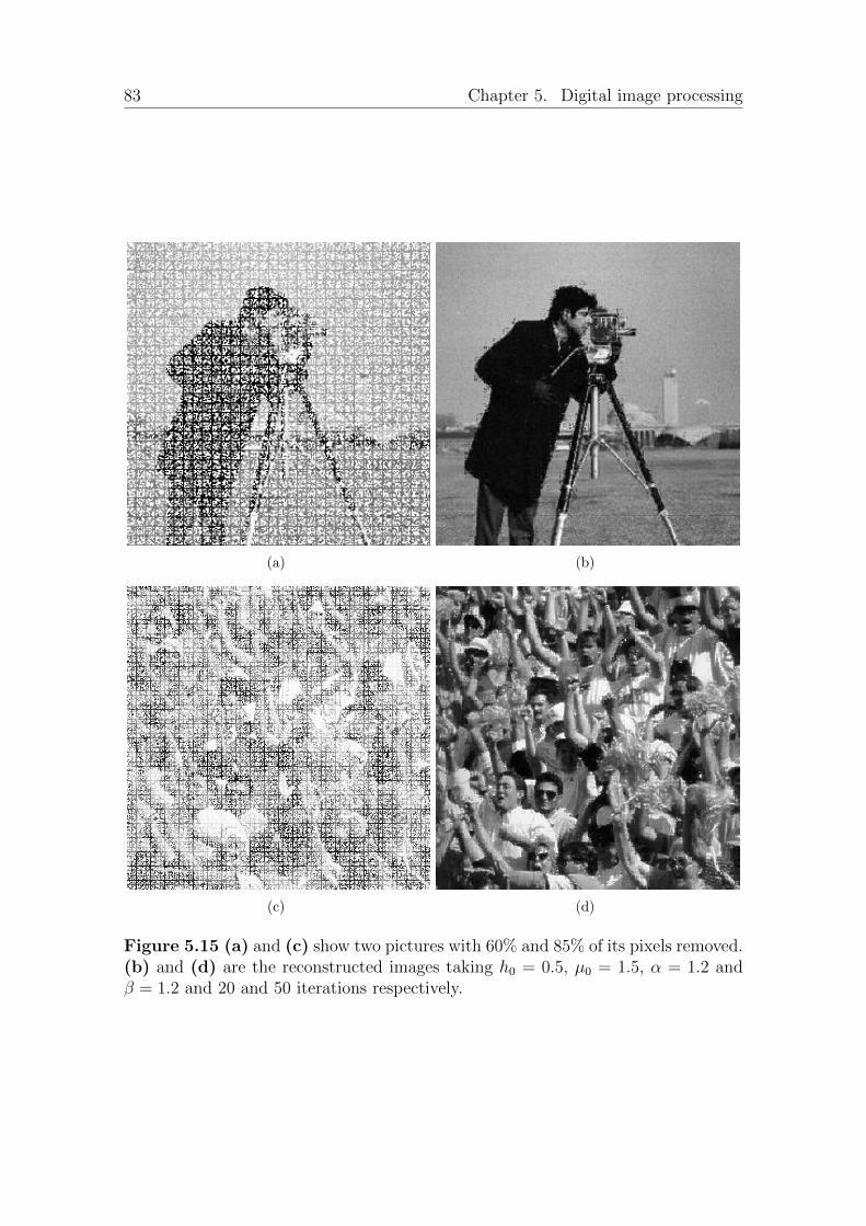
83 Chapter 5. Digital image processing
(a) (b)
(c) (d)
Figure 5.15 (a) and (c) show two pictures with 60% and 85% of its pixels removed.(b) and (d) are the reconstructed images taking h0 = 0.5, µ0 = 1.5, α = 1.2 andβ = 1.2 and 20 and 50 iterations respectively.

5.6. Image reconstruction 84
(a) (b) (c)
(d) (e) (f)
(g) (h) (i)
(j) (k) (l)
Figure 5.16 Pictures (d), (e), (f), (j), (k) and (l) are the reconstructions of (a),(b), (c), (g), (h) and (i) respectively. The parameters used are 100 iterations,h0 = 0.5, µ0 = 1, α = β = 1.2 and the squares are of size 10× 10 pixels.

Appendix
Along Chapter 5 we have developed different instances of digital image processingand, in each of them, the approaches set were illustrated by means of differentexamples. In the appendix we present the codes of the functions developed so asto implement such strategies. These functions, which are programmed in Matlab,were used to carry out all the examples appearing in the already mentioned chapter.
The aim of Section 5.3 was to obtain the edges of a given image. In order toachieve so we created a function, EdgeDetect, such that given an input image anda mask computes the filter associated to the latter and implements equation (5.2.4).The code is as follows.
function EdgeDetect (Im ,Mk)Im=imread (Im) ;Im=im2double (Im) ;i f s ize (Im , 3 ) ˜=1
Im=rgb2gray (Im) ;endM=s ize (Im , 1 ) ;N=s ize (Im , 2 ) ;
ImExt=[Im Im Im ; Im Im Im ; Im Im Im ] ;f i l t e r=zeros (3∗M,3∗N) ;a=(s ize (Mk, 1 )−1) /2 ;b=(s ize (Mk, 2 )−1) /2 ;f i l t e r (3∗M−a :3∗M,3∗N−b :3∗N)=Mk( 1 : a+1 ,1:b+1) ; %bottom r i g h tf i l t e r (3∗M−a :3∗M, 1 : b)=Mk( 1 : a+1,b+2:2∗b+1) ; %bottom l e f tf i l t e r ( 1 : a , 1 : b )=Mk( a+2:2∗a+1,b+2:2∗b+1) ; %top l e f tf i l t e r ( 1 : a , 3∗N−b :3∗N)=Mk( a+2:2∗a+1 ,1:b+1) ; %top r i g h tf i l t e r=sqrt (M∗N) ∗ f i l t e r ;
FourTransImExt=f f t2 ( ImExt ) /sqrt (M∗N) ;FourTransFi l ter=f f t2 ( f i l t e r ) /sqrt (M∗N) ;Conv=sqrt (M∗N) ∗ i f f t 2 ( FourTransImExt .∗ FourTransFi l ter ) ;Fi l t Im=Conv(M+1:2∗M,N+1:2∗N) ;imshow ( Fi l t Im )end
Notice that we regard images as elements of `2(ZM×ZN), so they should be extendedperiodically (as shown in line 10). Therefore, the computations are done with finitematrices of sizes 3M × 3N . However, the result that we are looking for is not thefiltered 3M × 3N matrix but the middle submatrix of size M ×N (line 23).
85

5.6. Image reconstruction 86
Moreover, this function works for any mask of length (2a + 1) × (2b + 1) fora, b ∈ Z, although all the masks considered in Section 5.3 where of size 3 × 3, thatis, a = b = 1.
In order to ease visualisation in the pictures shown in Figure 5.2 and 5.3, weadded the command
Fi l t Im=5.5∗ log(1+Fi l t Im ) ;
and
Fi l t Im=7.5∗ log(1+Fi l t Im ) ;
before the imshow respectively. Its purpose was to extend a narrow range of inten-sity levels located near 1 since, otherwise, the edges were too light.
Observe that this function is very general because it computes the convolution ofan image with the filter associated to the input mask. Since we were just interestedin edge detection, we executed it for the particular masks associated to that task.
In order to eliminate periodic noise (Section 5.4), we generated a function,PerNoise, such that, given the noisy picture and the notch, it performs the fil-tering and shows the result.
function PerNoise (NoisyIm , Notch )i f i s c h a r ( NoisyIm )==1
NoisyIm=imread (NoisyIm ) ;endNoisyIm=im2double ( NoisyIm ) ;i f s ize (NoisyIm , 3 ) ˜=1
NoisyIm=rgb2gray (NoisyIm ) ;endM=s ize (NoisyIm , 1 ) ;N=s ize (NoisyIm , 2 ) ;
FourTrans=f f t2 ( NoisyIm ) /sqrt (M∗N) ;Recovered=sqrt (M∗N) ∗ real ( i f f t 2 ( i f f t s h i f t (Notch .∗ f f t s h i f t ( FourTrans ) ) ) ) ;imshow ( Recovered )end
In our case, the degraded picture seen in Figure 5.6 was created by adding periodicnoise to the original one. The procedure was
eta1=zeros (M,N) ;eta2=zeros (M,N) ;for m=1:1:M
for n=1:Neta1 (m, n)=0.5∗ sin (2∗pi ∗200∗(m−1)/M) ;eta2 (m, n)=0.5∗ sin (2∗pi ∗200∗(n−1)/N) ;
endendeta=eta1+eta2 ;NoisyIm=Im+eta ;
where Im is the original grey-scaled image expressed as a matrix with values in [0, 1].Finally, the notch, which is shown in Figure 5.9 (a), was constructed as follows

87 Chapter 5. Digital image processing
CtOf=5; % cut−o f f f requencyNotch=zeros (M,N) ;for p=1:M
for q=1:NA=norm ( [ p−M/2−200 q−N/2 ] , 2 ) ˆ2 ;B=norm ( [ p−M/2+200 q−N/2 ] , 2 ) ˆ2 ;C=norm ( [ p−M/2 q−N/2−200] ,2) ˆ2 ;D=norm ( [ p−M/2 q−N/2+200] ,2) ˆ2 ;Notch (p , q )=(1−exp(−A/(2∗CtOfˆ2) ) )∗(1−exp(−B/(2∗CtOfˆ2) ) )∗(1−exp
(−C/(2∗CtOfˆ2) ) )∗(1−exp(−D/(2∗CtOfˆ2) ) ) ;end
end
Notice that the distances considered are slightly different than the ones seen inequation (5.4.2) due to the fact that matlab indexes matrices beginning at 1, notat 0.
In Section 5.5 we saw how to filter an image that had been degraded by a linearand translation-invariant transformation whose corresponding filter H (following thenotation introduced then) can be modelled. In order to perform such filtering, wedesigned a function, BlurRed, that follows the strategy shown in equation (5.5.4).The inputs are the noisy picture, the shifted model H and the cut-off value for thepatch function.
function BlurRed (NoisyIm , HShift , CtOf )i f i s c h a r ( NoisyIm )==1
NoisyIm=imread (NoisyIm ) ;endNoisyIm=im2double ( NoisyIm ) ;i f s ize (NoisyIm , 3 ) ˜=1
NoisyIm=rgb2gray (NoisyIm ) ;endM=s ize (NoisyIm , 1 ) ;N=s ize (NoisyIm , 2 ) ;
Patch=zeros (M,N) ;for p=1:M
for q=1:NPatch (p , q )=exp(−norm ( [ p−M/2 q−N/2 ] , 2 ) ˆ2/(2∗CtOfˆ2) ) ;
endend
FourSpec=f f t2 ( NoisyIm ) /sqrt (M∗N) ;Recovered=sqrt (M∗N) ∗ real ( i f f t 2 ( i f f t s h i f t ( Patch .∗ f f t s h i f t ( FourSpec ) . /
HShi ft ) ) ) ;imshow ( Recovered )
end
The examples that we worked on consisted in images degraded due to atmosphericturbulence. Therefore, according to equation (5.5.5), the second input of the func-tion had to be
k=0.0025;

5.6. Image reconstruction 88
HShift=zeros (M,N) ;for p=1:M
for q=1:NHShift (p , q )=exp(−k ∗ ( ( p−M/2)ˆ2+(q−N/2) ˆ2) ˆ(5/6) ) ;
endend
In fact, the noisy image was obtained by applying H to the Fourier Transform ofthe original image and then computing its Inverse Fourier Transform. That is
FourIm=f f t2 (Im) /sqrt (M∗N) ;NoisyIm=sqrt (M∗N) ∗ real ( i f f t 2 ( i f f t s h i f t ( f f t s h i f t (FourIm) .∗ HShift ) ) ) ;
where Im is the original image and HShift is the filter defined above. Finally, asdiscussed in the section itself, the cut-off chosen for Figure 5.11 (a) was 125 whereasfor Figure 5.11 (b) the patch was a constant matrix with all its components equalto 1. Therefore, in order to filter the latter we can execute the function taking alarge enough cut-off or we can modify it by suppressing the Patch.
Finally, in Section 5.6 we gave an algorithm for reconstructing an image withmissing pixels. In order to implement it, we designed a function, Reconstruction,that removes s pixels (uniformly distributed) of a given image and then reconstructsit. Since, as already mentioned in Section 5.6, the recovery is carried out in eachof the 8× 8 blocks that composes the picture, we defined another function which iscalled by the first one, BlckRecons, that adds noise and restores each of the blocks.The notation for the parameters is the one introduced in the already mentionedsection.
function Reconstruct ion (Im , s , i t e r , h 0 , mu 0 , alpha , beta )Im=imread (Im) ;i f s ize (Im , 3 ) ˜=1
Im=rgb2gray (Im) ;endIm=im2double (Im) ;M=s ize (Im , 1 ) ;N=s ize (Im , 2 ) ;
i f f loor (M/8)==M/8auxM=M/8 ;
elseauxM=f loor (M/8)+1;
endi f f loor (N/8)==N/8
auxN=N/8 ;else
auxN=f loor (N/8)+1;end
ImExt=[Im Im ; Im Im ] ;Blocks=c e l l (auxM, auxN) ;BlocksRec=c e l l (auxM, auxN) ;BlocksNoisy=c e l l (auxM, auxN) ;for i =1:auxM

89 Chapter 5. Digital image processing
for j =1:auxNBlocks i , j=ImExt (8∗ ( i −1)+1:8∗( i −1)+1+7,8∗( j−1)+1:8∗( j−1)+1+7) ;[ BlocksNoisy i , j , BlocksRec i , j ]=BlckRecons ( Blocks i , j , s , i t e r
, h 0 , mu 0 , alpha , beta ) ;end
end
NoisyIm=ce l l 2mat ( BlocksNoisy ) ;RecIm=ce l l 2mat ( BlocksRec ) ;NoisyIm=NoisyIm ( 1 :M, 1 :N) ;RecIm=RecIm ( 1 :M, 1 :N) ;
subplot ( 1 , 2 , 1 ) ; imshow (NoisyIm ) , t i t l e ( ’ Degraded ’ )subplot ( 1 , 2 , 2 ) ; imshow (RecIm) , t i t l e ( ’ Reconstructed ’ )end
where
function [ BlVis , y]=BlckRecons ( Block , s , i t e r , h 0 , mu 0 , alpha , beta )M=8;N=8;Rows=f loor (1+(M−1)∗rand (1 , s ) ) ;Colms=f loor (1+(N−1)∗rand (1 , s ) ) ;NoisyBl=Block ;BlVis=Block ;for i =1: s
NoisyBl (Rows( i ) ,Colms ( i ) )=0;BlVis (Rows( i ) ,Colms ( i ) )=1;
end
%Gradient descent a l gor i thmy=NoisyBl ;mu=mu 0 ;for t=1: i t e r
Grad=zeros (M,N) ;for i =1: s
a=Rows( i ) ;b=Colms ( i ) ;Aux=zeros (M,N) ;Aux(a , b)=h 0 ;X pos=f f t2 ( y+Aux) /sqrt (M∗N) ;X neg=f f t2 (y−Aux) /sqrt (M∗N) ;Grad (a , b)=1/(2∗h 0 ) ∗(sum(sum(abs ( X pos ) ) )−sum(sum(abs ( X neg
) ) ) ) ;endy=y−mu∗Grad ;
h 0=h 0/alpha ;mu=mu/beta ;
endend
Notice that the given image is extended periodically. Finally, we implemented afunction, QuadRec, that adds a square of size quad × quad to a given image in a

5.6. Image reconstruction 90
random location and uses the gradient descent algorithm to restore it.
function QuadRec(Im , i t e r , h 0 , mu 0 , alpha , beta ,quad)Im=imread (Im) ;i f s ize (Im , 3 ) ˜=1
Im=rgb2gray (Im) ;endIm=im2double (Im) ;M=s ize (Im , 1 ) ;N=s ize (Im , 2 ) ;
Rows=f loor (1+(M−quad+1)∗rand ) ;Colms=f loor (1+(N−quad+1)∗rand ) ;NoisyIm=Im ;ImVis=Im ;NoisyIm (Rows :Rows+quad , Colms : Colms+quad)=0;ImVis (Rows : Rows+quad , Colms : Colms+quad)=1;
%Gradient descent a l gor i thmy=NoisyIm ;mu=mu 0 ;
for t=1: i t e rGrad=zeros (M,N) ;
for i=Rows :Rows+quadfor j=Colms : Colms+quada=i ;b=j ;Aux=zeros (M,N) ;Aux(a , b)=h 0 ;X pos=f f t2 ( y+Aux) /sqrt (M∗N) ;X neg=f f t2 (y−Aux) /sqrt (M∗N) ;Grad (a , b)=1/(2∗h 0 ) ∗(sum(sum(abs ( X pos ) ) )−sum(sum(abs ( X neg
) ) ) ) ;end
endy=y−mu∗Grad ;h 0=h 0/alpha ;mu=mu/beta ;
endsubplot ( 1 , 2 , 1 ) ; imshow ( ImVis ) , t i t l e ( ’ Degraded ’ )subplot ( 1 , 2 , 2 ) ; imshow (y ) , t i t l e ( ’ Reconstructed ’ )end

Bibliography
[1] A. Draganic, I. Orovic and S. Stankovic, On some common compressive sens-ing recovery algorithms and applications, Facta Universitatis, Series: Elec-tronics and Energetics 30 (2017), no. 4, 477–510.
[2] M. W. Frazier, An Introduction to Wavelets Through Linear Algebra, Springer,1999.
[3] R. C. Gonzalez and R. E. Woods, Digital Image Processing, Pearson PrenticeHall, 2008.
[4] R. C. Gonzalez, R. E. Woods and S. L. Eddins, Digital Image ProcessingUSING MATLAB, Gatesmark, 2009.
[5] R. E. Hufnagel and N. R. Stanley, Modulation Transfer Function Associatedwith Image Transmission Through Turbulent Media, J. Opt. Soc. Amer. 54(1964), 52–61.
[6] I. Orovic, V. Papic, C. Ioana, X. Li, and S. Stankovic, Compressive Sens-ing in Signal Processing: Algorithms and Transform Domain Formulations,Mathematical Problems in Engineering 2016 (2016), 1–16.
[7] I. Stankovic, Recovery of Images with Missing Pixels using a Gradient Com-pressive Sensing Algorithm, (2014), https://arxiv.org/abs/1407.3695.
[8] J. S. Walker, Fast Fourier Transforms, CRC Press, 1996.
91