the discriminatory nature of speciÞc tariffs and her email address is [email protected]....

The Discriminatory Nature of Specific Tariffs

Sohini Chowdhury

This paper quantifies the distortions from specific tariffs levied by the EU. The most-favored-nation (MFN) specific tariffs levied by the EU translate into higher tariff bar-riers for poor countries exporting low price goods. We show that for poor countries,these higher tariff barriers from specific tariffs offset the gains from preferentialtariffs. We apply a two-stage analysis to show that the specific tariffs levied by the EUon its agricultural imports wash away more than half of the welfare benefits enjoyedby the Sub-Saharan African countries from EU preferential tariffs. Our results providethe first quantitative estimate of the distortions associated with specific tariffs.JEL codes: F13, F14, O12, Q17

The most-favored-nation (MFN) clause, a key feature of the WTO agreement,requires that each WTO member treat its trading partners equally by levying acommon MFN tariff on every imported tariff line. But while a MFN specifictariff (e.g. $2 per ton) conforms to this non-discrimination principle in paper,it violates this principle in spirit. In fact, specific tariffs discriminate againstimports from poor countries. We can identify two channels for this. First, poorcountries tend to have lower export prices compared to rich countries (Schott,2004);1 this means that when poor and rich exporters face the same level ofspecific tariff, poor exporters face a higher ad valorem equivalent (AVE).2

Sohini Chowdhury did this analysis towards her doctoral dissertation at the Krannert School of

Management, Purdue University (403 W State St, West Lafayette, IN 47907). She is currently an

economist at Moody’s Analytics Inc. (121 N Walnut Street, Suite 500, West Chester, PA 19380). She is

grateful to Chong Xiang, Thomas Hertel, David Hummels and Luca Salvatici for excellent guidance,

and to Badri Narayanan Gopalakrishnan for useful comments. Her phone number is þ1 (410) 402-

4462, and her email address is [email protected].

1. Schott (2004) analyzed US manufacturing imports for the year 2001 and found a significant positive

correlation between the per capita GDP of exporters and the unit value of their exports. He concluded that

rich countries utilize their comparative advantage in skill and capital to supply higher quality and higher

priced varieties. Abd-El-Rahman (1991) shows that unit value differences reveal quality differences, even at

the detailed ten-digit HS level. Fontagne et al. (1997) and Greenaway et al. (2001) show that vertical

specialization is among the most salient features of trade between European countries.

2. The AVE of a specific tariff expresses the specific tariff on a commodity as a percentage of the price of

the commodity. This means that the same specific tariff of $2/ton on rice translates into a higher AVE, say

50%, for rice imported from Bangladesh and a lower tariff equivalent, say 10%, for rice imported from Japan.

This effect is seen with any per-unit specific price rise, arising either from an unit transport cost (Alchian

and Allen, 1964; Hummels and Skiba, 2004) or from an import quota (Falvey, 1979; Boorstein and Feenstra,

1987).

THE WORLD BANK ECONOMIC REVIEW, VOL. 26, NO. 1, pp. 147–163 doi:10.1093/wber/lhr036Advance Access Publication July 12, 2011# The Author 2011. Published by Oxford University Press on behalf of the International Bankfor Reconstruction and Development / THE WORLD BANK. All rights reserved. For permissions,please e-mail: [email protected]

147

Pub

lic D

iscl

osur

e A

utho

rized

Pub

lic D

iscl

osur

e A

utho

rized

Pub

lic D

iscl

osur

e A

utho

rized

Pub

lic D

iscl

osur

e A

utho

rized

Pub

lic D

iscl

osur

e A

utho

rized

Pub

lic D

iscl

osur

e A

utho

rized

Pub

lic D

iscl

osur

e A

utho

rized

Pub

lic D

iscl

osur

e A

utho

rized

WB456286

Typewritten Text

81288

Second, specific tariffs are concentrated on agricultural commodities3 whichform the bulk of poor country’s exports (Gibson et al., 2001;4 Hoekman et al.,2002). Our initial data analysis shows that in 2004, nearly half (48%) of theglobal agricultural imports were sourced from poor countries. While the discri-minatory effects of specific tariffs have been discussed in the literature (Gibsonet al., 2001; Von Kirchbach and Mondher, 2003; Bouet et al., 2004), there hasbeen no quantitative estimate of the welfare loss faced by poor countries fromsuch tariffs. In this paper we provide an estimate of the additional welfare lossfrom specific tariffs, vis-a-vis ad valorem tariffs, accruing to poor countries.Additionally, to get a better sense of the size of this loss, we express the loss asa percentage of the welfare gain enjoyed by poor countries from the tariff pre-ferences granted to them by rich countries. Article XXIV of the GATT/WTOtogether with the Enabling Clause,5 permit exemptions to the MFN obligationand create a legal basis for the formation of Preferential Trade Agreements.These PTAs can be bilateral/reciprocal tariff preferences like Free TradeAgreements or Customs Unions, or unilateral/non-reciprocal tariff preferencesextended from developed to developing countries like the Generalized Systemof Preferences (GSP), and its extensions like the Everything but Arms (EBA)6

initiative by the EU and the African Growth and Opportunities Act (AGOA)7

by the US.Results show that more than half the welfare gains enjoyed by the

Sub-Saharan8 countries (SSA) from the preferences granted to them by the EUare taken away by the specific tariffs levied by the EU. In other words, whileon one hand the EU grants preferences to poor countries through lower tariffrates, on the other hand it takes away the benefits of these preferences throughspecific tariffs.

To arrive at our results, we use a partial equilibrium model considering onlythe preferential and specific tariffs levied by the EU on its agricultural importsfrom Sub-Saharan Africa. We follow a two-stage procedure, sequentially elimi-nating preferential tariffs and specific tariffs by the EU. In Stage 1, we eliminate

3. Our analysis in Section I shows that specific tariffs were concentrated on agricultural imports

whether analyzed in terms of the number of tariff lines, the tariff rates, or the AVEs.

4. Gibson et al. (2001) states that approximately 44 % of agricultural tariff-lines in the US and EU

are specified in non-ad valorem terms. The reasons include the increased protection that a non-ad

valorem tax provides against large drops in import prices and the lack of transparency associated with

these rates, which helps conceal the level of protection.

5. Decision on Differential and More Favourable Treatment, Reciprocity, and Fuller Participation of

Developing Countries, GATT Document L/4903, 28 November 1979, BISD 26S/203

6. This initiative came into effect in 2001. Under this, the EU grants duty free access to imports of

all products that originate in LDCs with the exception of arms and munitions.

7. This act came into effect in 2000. Under this the US extended preferences to 37 African

countries, providing duty free access to agricultural commodities.

8. EU includes the 25 member countries of the European Union in 2004. SSA includes 50 countries

(all of Africa – South Africa – a few small dependencies – the six North African countries of West

Sahara, Morocco, Algeria, Libya, Tunisia and Egypt).

148 T H E W O R L D B A N K E C O N O M I C R E V I E W

preferential tariffs by moving from the preferential tariff schedule to the MFNtariff schedule. In Stage 2, we eliminate specific tariffs by moving from theMFN tariff schedule to the mean ad valorem equivalent tariff schedule, wherethe mean is taken over all exporters for each importer-commodity pair. Wethen compare the welfare losses from each stage.

There is a large literature that analyzes the welfare gains/losses from tradeagreements.9 In comparison, our paper disentangles the effects of specifictariffs and trade agreements and compares the welfare loss from specific tariffsto the welfare gains from preferential tariffs. There is also a large literature thatcalculates the distortions from tariffs.10 In comparison, our paper calculatesthe additional distortion from specific tariffs vis-a-vis ad valorem tariffs. Wedefine the mean ad valorem tariff equivalent as a benchmark11 to calculate theadditional loss from specific tariffs.

The rest of our paper is organized as follows: We present some preliminarydata analysis in Section I and discuss the general research methodology inSection II. Sections III and IV describe the model and data, and the results areanalyzed in Section V. Section VI presents some robustness checks and SectionVII concludes.

I . P R E L I M I N A RY D ATA A N A LY S I S

We use trade and tariff data for the year 2004 from the Comtrade andMAcMapHS6v2.02 databases respectively. The data sources are discussed indetails in Section IV. Figure 1 shows that globally, specific tariffs are concen-trated in the trade of agricultural commodities. 11% of all bilateral tariff linesin agriculture face specific tariffs, compared to only 1.6% of the bilateral tarifflines in non-agriculture and 2.4% of all bilateral tariff lines. In terms of thenumber of tariff lines, 65% of all the bilateral tariff lines facing specific tariffsare agricultural commodities. In terms of tariff rates, 67% of the value of allbilateral specific tariff rates (in $ per ton) are on agricultural commodities.Based on these data analyses, the rest of our paper will focus on specific tariffson agricultural imports alone. The data identifies Iceland, Vanatua,Switzerland and Norway as countries with high specific tariffs on their agricul-tural imports; and Kenya, Vietnam, Kazakhstan and Uzbekistan as countriesfacing high ad valorem equivalents of specific tariffs on their agricultural

9. These studies are either in a partial equilibrium framework using some variant of the gravity

equation (Baier et al., 2007; Carrere, 2006) or in a general equilibrium framework (Bouet and Laborde,

2009; Anderson et al., 2006, Francois et al., 2005)

10. Feenstra (1995), Anderson (1998), Kee et al. (2009), Irwin (2010), Lloyd et al. (2010) to name

a few.

11. Boorstein and Feenstra (1987) do something similar when they calculate the ‘excess cost’ of the

US steel import quotas during 1969–74. They define as the benchmark the ad valorem tariff which has

the same effect on aggregate import price as the quota.

Chowdhury 149

exports. Figure 2 shows that poor exporters, on average, face higher advalorem equivalents of specific tariffs.

We check this claim further by testing, similar to Schott (2004), the relation-ship between an exporter’s per capita GDP and the unit values of its

FIGURE 1. AVEs of Specific Tariffs by Commodity

Notes: The AVEs corresponding to each HS2 is obtained by taking a simple average over alltariff lines for all importers, within each HS2. HS Chapter: 06 is ‘live trees & plants’; HSChapter: 24 is ‘tobacco’; HS Chapter: 01-24 are agricultural commodities.

Source: Authors’ analysis based on data sources discussed in the text.

FIGURE 2. AVEs of Specific Tariffs in Agriculture by Exporter

Notes: Kenya (KEN), Kazakhstan (KGZ), Uzbekistan (UZB), Vietnam (VNM), Papua NewGuinea (PNG), Mongolia (MNG).



agricultural exports. We estimate the following regression pooling across allexporters ( j) and all importers (i), for all agricultural goods (k) (HSChapter , ¼24), with HS6 commodity fixed effects

ln uvijk ¼ aik þ b lnGDP

L

� �j

þjik ð1Þ

where, aik is the importer-by-commodity fixed effect, uvijk is the unit value ofgood k imported into i from j, (GDP/L)j is the per capita GDP of exporter j andjik is the error term. For unit values, we use the Exporter Reference Group UnitValues (ERGUVs), which are computed as the weighted median unit value ofworldwide exports from an exporter’s reference group (Bouet et al., 2004).12

Our estimation results, presented in Table 1, suggest that on average, doublingthe per capita GDP of exporters increases the ERGUVs of their exports by7.7%. The significant positive correlation between the exporter’s unit value andper capita GDP corroborates the claim that on average, the ad valorem equiva-lents of MFN specific tariffs are higher for poor country exporters. It is thisfeature of specific tariffs that bias them against poor exporters.

I I . R E S E A R C H M E T H O D O LO GY

While specific tariffs increase the effective tariff rates faced by poor exporters,preferential tariffs lower these rates by granting poor exporters tax concessions.So the welfare losses faced by poor exporters from specific tariffs can be ana-lyzed only if we control for the welfare gains from the preferential tariffs theyface.13 We use a two-stage experiment to disentangle these two effects. InStage 1, we eliminate preferential tariffs by removing all preferences granted byrich importers in agriculture. This is achieved by moving from the rich impor-ter’s preferential tariff rates (which we denote by tp) to their MFN tariff rates.

12. Bouet et al. (2004) assign each reporting country to a reference group of similar countries using

a hierarchical clustering analysis based on GDP per capita (in terms of PPP) and trade openness. They

label the five resulting groups as: (1) richest countries; (2) high openness, middle income countries; (3)

low openness, middle income countries; (4) high openness, low income countries; (5) low openness, low

income countries. The full set of countries and reference groups is provided in Appendix A1 of their

paper. They calculate ERGUVs using "weighted" medians assuming that each UV repeats as many

times as the underlying trade flow contains dollars. For robustness, the UVs are computed based on

three-year-average trade flows (across the 2000–2002 period). Outliers are filtered by truncating to the

top or bottom limit, any ratio of ERGUVs to the world median unit value which fall outside the bracket

[1/3; 3]. A sequential procedure is used to fill missing values for reference groups: any blank is

substituted by the value of the closest reference group.

13. This is especially relevant given the recent proliferation of PTAs. In 2008, there were over 350

PTAs (Bhagwati, 2008) suggesting that the rich countries now grant MFN tariffs to only a handful of

countries. The EU applies its MFN tariffs to only six countries – Australia, New Zealand, Canada,

Japan, Taiwan and the US – with all other countries enjoying more favorable tariffs. This has prompted

Bhagwati to suggest that the MFN tariff should be more appropriately renamed as the LFN (Least

Favored Nation) tariff (Bhagwati, 2008)

Chowdhury 151

Now while the MFN tariff rates are the same for all exporters correspondingto each rich importer-commodity pair, their ad valorem equivalents (which wedenote by tm) are not, since these MFN rates also include specific tariffs. InStage 2 therefore, we convert the specific tariffs levied by rich importers onagriculture to ad valorem tariffs. This is achieved by moving from the advalorem equivalents of MFN tariff rates (tm) to the mean ad valorem equiva-lents across all exporters (which we denote by tc). The counterfactual mean advalorem tariff tc is truly MFN since it is uniform across exporters for eachimporter-commodity pair. We construct tc for each importer-commodity pairaccording to Equation 18, as the average ad valorem equivalent faced by allexporters, weighted by the product of the price elasticity of import demandand free-trade imports, following Leamer (1974). We clarify the intuitionbehind tp, tm and tc in Table 2. The table shows the ad valorem equivalents oftariffs levied by Switzerland on its import of raw cane sugar from Japan andGuatemala. tp denotes the actual tariffs levied and includes both preferentialand specific tariffs. Due to the preferential tariff benefits enjoyed by the poorcountry Guatemala, it faces a lower (in this case, a zero) tp than Japan. tm isthe ad valorem equivalent of the MFN tariff rates levied by Switzerland anddoes not include preferential tariffs. Although the MFN tariff rates are identicalacross exporters, their ad valorem equivalents (tm) are not, due to the presenceof specific tariffs. In particular, due to the lower price of Guatemala exports,Guatemala faces a higher tm than Japan. To even out the non-MFN effects ofspecific tariffs across Guatemala and Japan, we construct the counterfactualtariff tc as the mean ad valorem tariff equivalent across all exporters. Having

TA B L E 2. An Illustration of the 2-Stage Procedure

Exporter

Ad Valorem Equivalents of Swiss import tariffs on Raw Cane Sugar

Stage 1 Stage 2tp ! tm ! tc

Guatemala 0.00 2.28 0.33Japan 0.10 0.10 0.33


TA B L E 1. Regression of Unit Values on Exporter Per Capita GDP

ln(p1) ln(p2)

ln(GDP/L) 0.077**(0.002)

0.121(0.061)

N 229640 229640


p1 ¼ ERGUV; p2 ¼ bilateral unit value. **p , 0.01


been stripped off the effects of specific tariffs, tc is the same across all expor-ters. Once we have the three tariff schedules tp, tm and tc, we compare thewelfare losses corresponding to each. We run both stages of the experimentunder a partial equilibrium model which considers only the EU’s tariff policytowards Sub-Saharan Africa.

I I I . M O D E L

We consider a simple world with the EU as the only importer. All countriesexporting to the EU are classified as either SSA (Sub-Saharan Africa) ornon-SSA. We consider only the trade in agricultural commodities. We selectthe particular combination of the EU and SSA because our data suggests thaton average, EU agricultural imports from SSA face high MFN specific tariffs(31.3%) and are significantly higher ($9.67 billion) than the imports of otherrich countries from SSA. Moreover, almost every EU agricultural tariff lineimported from SSA benefits from some tariff preference (only 17 out of the516 tariff lines face no preference). These make the EU and SSA perfect candi-dates for our model. We use the model to compute the proportion of thebenefits enjoyed by SSA from EU preferential tariffs that are taken away by EUspecific tariffs.

Consider the import of commodity k from country j into the EU given by

q jk ¼ adjkp�sk

jk ð2Þ

Consider the export of commodity k from country j to the EU given by

q jk ¼ asjkpSk

jk ð3Þ

where, j [ fall exportersg is the exporter index, k [ fagricultural tariff linesgis the commodity index, sk is the own price elasticity of import demand ofgood k in the EU, and Sk is the own price elasticity of export supply of good kfrom the rest of the world as faced by the EU. adjk and asjk are shift parameterscorresponding to the import demand and export supply curves respectively.From the Comtrade dataset, we obtain data on bilateral c.i.f prices (psjk) andimport quantitities (q0jk) for the EU. All other prices and quantities areexpressed in terms of these values and elasticities.

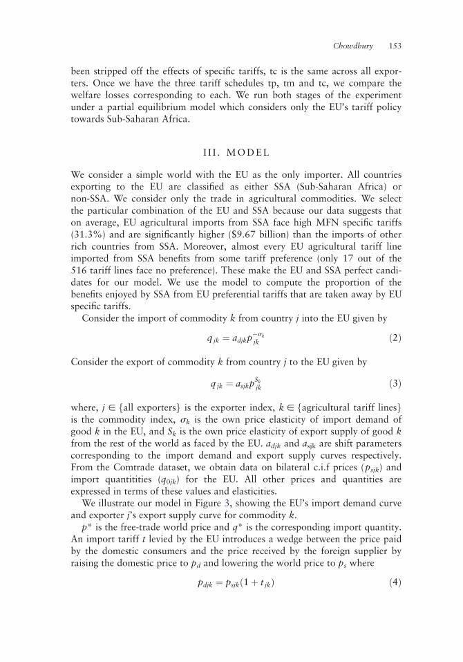
We illustrate our model in Figure 3, showing the EU’s import demand curveand exporter j’s export supply curve for commodity k.

p* is the free-trade world price and q* is the corresponding import quantity.An import tariff t levied by the EU introduces a wedge between the price paidby the domestic consumers and the price received by the foreign supplier byraising the domestic price to pd and lowering the world price to ps where

pdjk ¼ psjkð1þ t jkÞ ð4Þ

Chowdhury 153

As Figure 3 shows, the distribution of the tariff incidence between the EU andthe exporter is determined by the import demand and export supply elasticitiessk and Sk. The post-tariff import quantity is q0. The EU faces an allocative effi-ciency loss from the import tariff due to the higher domestic price and lowerimport, and a terms of trade gain due to the lower price it pays for its import.So the net welfare loss faced by the EU from the import tariff t is equal to theallocative efficiency loss it faces net of the terms of trade gain. SSA faces anallocative efficiency loss due to lower exports, and a terms of trade loss (equiv-alent to the terms of trade gain faced by the EU) due to the lower price itreceives on its export. So the net welfare loss faced by SSA from the importtariff t is equal to the sum of its allocative efficiency loss and terms of tradeloss. It is important to note that all losses are expressed with respect to the freetrade i.e. zero tariff scenario.

The welfare loss in EU and an exporting country j, from a tariff t levied bythe EU on commodity k is derived as follows:

From Figure 3, ignoring the subscripts, we have

q0 ¼ adp�sd ¼ aspSs ð5Þ

From (4) and (5), we have

adp�ss ð1þ tÞ�s ¼ aspSs ð6Þ

FIGURE 3. Welfare Loss

Source: Authors’ analysis based on model discussed in the text.


Rearranging (6), we have

ad

as¼ ð1þ tÞspSþs

s ð7Þ

From Figure 3 we also have

q� ¼ adp��s ¼ asp�S ð8Þ

From (8), we have

ad

as¼ p�ðSþsÞ ð9Þ

Combining (7) and (9), we have

ð1þ tÞspSþss ¼ p�ðSþsÞ ð10Þ

Rearranging (10), we have

p� ¼ psð1þ tÞs

sþS ð11Þ

From (11), (8) and (5), we have

q� ¼ q0ð1þ tÞsSsþS ð12Þ

From Figure 3, AE loss in the EU

¼Ðq�q0

pðqdÞdq� ðq� � q0Þp�

¼Ðq�q0

qad

� ��1s

dq� ðq� � q0Þp�

¼ ðadÞ1s q1�1

s

1�1s

��q�q0

�ðq� � q0Þp�

¼ ss�1 ðadÞ

1s q�

s�1s � q

s�1s

0

h i� ðq� � q0Þp�

Substituting the values of q* and p* from (12) and (11) respectively, we have

Chowdhury 155

AE loss in the EU

¼ s

s� 1ðq0ps

dÞ1s q

s�1s

0

� �ð1þ tÞ

Sðs�1ÞsðsþSÞ � 1

h i

� q0 ð1þ tÞsSsþS � 1

h ipsð1þ tÞ

ssþS

¼ s

s� 1psð1þ tÞq0 ð1þ tÞ

Sðs�1ÞsðsþSÞ � 1

h i

� q0psð1þ tÞsð1þSÞsþS þ q0psð1þ tÞ

ssþS

¼ psq01

s� 1ð1þ tÞ

sð1þSÞsþS � s

s� 1ð1þ tÞ þ ð1þ tÞ

ssþS

� �

ð13Þ

From Figure 3, AE loss in the exporter j

¼ ðq� � q0Þp� �Ð q�q0

pðqsÞdq

¼ ðq� � q0Þp� �Ð q�q0

qs

as

� �1S

dq

¼ ðq� � q0Þp� �S

Sþ 1a�1

Ss q�

Sþ1S � q

Sþ1S

0

h i

Substituting the values of q* and p* from (12) and (11) respectively, we haveAE loss in exporter j

¼ q0 ð1þ tÞsSsþS � 1

� �psð1þ tÞ

ssþS � S

Sþ 1a�1

Ss

qSþ1

S

0 ð1þ tÞsð1þSÞsþS � q

Sþ1S

0

h i

¼ psq0S

Sþ 1� ð1þ tÞ

ssþS þ 1

Sþ 1ð1þ tÞ

sð1þSÞsþS

� �ð14Þ

TOT gain in the EU/loss in exporter j

¼ ð p� � psÞq0

Substituting the value of p* from (11), we get


TOT gain in the EU/loss in exporter j

¼ psq0 ð1þ tÞs

sþS � 1h i

ð15Þ

Finally we have,Net welfare loss in EU

¼ SjSkq0jkpsjk1

sk � 1ð1þ t jkÞ

skð1þSkÞskþSk � sk

sk � 1ð1þ t jkÞ þ ð1þ t jkÞ

skskþSk

� �

AE LOSS

�SjSkq0jkpsjk ð1þ t jkÞsk

skþSk � 1h i

TOT LOSS

ð16Þ

Net welfare loss in exporter j

¼ Skq0jkpsjkSk

ðSkþ1Þþ 1

ðSk þ 1Þ ð1þ t jkÞskðSkþ1Þ

Skþsk � ð1þ t jkÞsk

skþSk

� �

AE LOSS

þPk

q0jkpsjk ð1þ t jkÞsk

skþSk � 1h i

TOT LOSS

ð17Þ

Then applying the available data to (16) and (17) we calculate the dollarvalues of the welfare loss corresponding to the three different tariff schedulestp, tm and tc. Using (16) and (17), we can also derive the allocative efficiencyloss and terms of trade loss corresponding to the special scenarios shown inTable 3.

TA B L E 3: Welfare Change Under Special Scenarios

Scenario Result

When tjk ¼ 0, for all j, k TOT loss and allocative efficiency loss for the EU is 0TOT loss and allocative efficiency loss for each

exporter is 0Welfare loss for the EU and all exporters is 0Although welfare loss is 0, welfare is not optimum

for the EU since there can be welfare gains frompositive TOT gains

When Sk ¼1 for all k, indicating a flatexport supply curve faced by the EU

The TOT gains for the EU and TOT losses for eachexporter is 0

When sk ¼1, for all k, indicating a flatimport demand curve faced by the EU

Allocative efficiency loss for the EU is 0


Chowdhury 157

I V. D ATA

Data on EU bilateral c.i.f.14 prices (ps) and the corresponding imports (q0) atthe six-digit Harmonized System are obtained from the Comtrade database forthe year 2004. Data on the ad valorem and specific components of EU MFNand preferential tariff rates for for the year 2004 are obtained from theMAcMap-HS6v2.02 database (Boumellassa et al., 2009). We construct the advalorem equivalents of specific tariffs by dividing the specific tariffs by theExporter’s Reference Group Unit Values. We denote by tp, the sum of the pre-ferential ad valorem tariff and the ad valorem equivalent of the preferentialspecific tariff. We denote by tm, the sum of the MFN ad valorem tariff and thead valorem equivalent of the MFN specific tariff. Finally, we constructthe mean ad valorem tariff equivalent tc for each importer-commodity pair asthe average tm over all exporters, weighted by the product of the price elastici-ties of import demand and free-trade imports (Leamer, 1974) as:

tcik ¼Sjsikq0ijkð1þ tmijkÞ�sik tmijk

Sjsikq0ijkð1þ tmijkÞ�sikð18Þ

where i [ fEUg is the importer index and all other notations follow the defi-nitions in Section III. The differences in the welfare loss corresponding to tpand tm show the effect of eliminating EU preferential tariffs on SSA agricul-tural imports. This is Stage 1 of our experiment. The differences in the welfareloss corresponding to tm and tc show the effect of converting EU specifictariffs on SSA agricultural imports to ad valorem tariffs. This is Stage 2 of ourexperiment. To avoid aggregation bias, we perform all tariff changes at theindividual country and tariff line level. The results are then aggregated for pres-entation and analysis.

Agricultural imports from SSA ($9.67 billion) constitute less than 10% oftotal EU imports. For agricultural exports to the EU, SSA faces a lower prefer-ential tariff (4.7%) when compared to non-SSA (9.3%). This is to be expected,since the EU extends preferential market access to agricultural imports fromSSA. But SSA faces a higher average ad valorem equivalent of MFN tariffs(14.7%) relative to non-SSA (11.8%); consistent with the hypothesis thatexports from SSA have lower unit values on average when compared to exportsfrom non-SSA. To compute the welfare loss, we also need data on the priceelasticities of import demand (s) and export supply (S) for the EU. We obtainthe former from Kee et al. (2008), and the latter from Broda et al. (2008)which contains estimates of the commodity-specific export supply elasticitiesfor the US. We apply these elasticities to the EU, assuming that the EU facesidentical elasticities.

14. Cost, insurance and freight (the price on which import tariff is applied)


V. R E S U LT S

We present the welfare changes from Stages 1 and 2 in Table 4. Stage 1 gener-ates an allocative efficiency loss in the EU and SSA equal to $578 million and$719 million respectively, and a terms of trade gain in the EU matched by anequivalent terms of trade loss in SSA of $1237 million. Non-SSA faces no tariffchange and therefore no welfare change. We attribute the higher allocative effi-ciency loss in SSA to the observation that the EU faces a relatively steep exportsupply curve compared to the import demand curve. The average exportsupply elasticity on agricultural goods faced by the EU is 1.92 and the corre-sponding import demand elasticity is -3.21. These relative elasticities alsoexplain the strong terms of trade effect relative to the allocative efficiencyeffect.15 In Stage 2, SSA gains $522 million and $729 million respectively interms of allocative efficiency and terms of trade due to lower tariff rates. TheEU faces an allocative efficiency gain of $389 million since it now levies amore uniform tariff across its exporters while maintaining the same trade-weighted average tariff rate.16 But the EU also faces a terms of trade loss fromlevying lower tariffs on SSA imports. This loss is partly compensated by thehigher tariffs on non-SSA imports resulting in a net terms of trade loss of $113million. The higher tariffs on non-SSA imports generate allocative efficiencyand terms of trade losses for non-SSA equivalent to $722 million and $616million respectively. So the uniform tariffs levied in Stage 2 essentially switchthe destinies of SSA and non-SSA. The combined results from Stages 1 and 2suggest that 64% of the welfare gains enjoyed by SSA from the preferential

TA B L E 4. Welfare Change. (US$ millions)

Region

Stage 1 Stage 2

AEChange

TOTChange

WelfareChange

AEChange

TOTChange

WelfareChange

EU 2578 1237 659 389 2113 276SSA 2719 21237 1956 522 729 1251Non-SSA 0 0 0 2722 2616 21338


15. This is consistent with the terms-of-trade argument (Bagwell et al., 2006) which shows that the

terms of trade changes resulting from tariff cuts are significantly large and play an important role in a

country’s decision to join a trade agreement. According to this argument, trade agreements are useful to

governments as a means of helping them escape from a terms-of-trade-driven Prisoners’ Dilemma.

Broda et al. (2008) provides an empirical support of this argument by showing that the tariff choices of

non-WTO countries reflect their ability to manipulate their terms of trade.

16. For a small importer, an increase in tariff dispersion increases the trade restrictiveness and

welfare loss. (Anderson et al., 2007; Feenstra, 1995; Irwin, 2010). In our large importer case, it

increases the allocative efficiency loss. This explains why trade agreements seek to lower both tariff

distortions and tariff peaks.

Chowdhury 159

tariffs on its agricultural exports to EU are washed away by the specific tariffslevied by the EU. The welfare loss to SSA from EU specific tariffs is equivalentto 12.7% of SSA agriculture exports to the EU. This finding highlights the dis-criminatory nature of specific tariffs. It suggests that we can add specific tariffsto the list of factors thought to be eroding away the effectiveness of non-reciprocal/unilateral trade agreements meant to expand trade and promotedevelopment in poor countries. This widely debated list includes other ‘cul-prits’ like limited product coverage, proliferation of regional trade agreements,attached side conditions and Rules of Origin.17

This model does not account for substitution across imported and domesticcommodities and across different imported varieties, and also ignores all inter-sectoral linkages and income effects. To capture these effects, we run the twostages of the experiment in a computable general equilibrium Global TradeAnalysis Project (GTAP) model (Hertel, 1997), analyzing simultaneously thetrade policy of multiple importers and exporters. The results, to be presented in aseparate working paper, suggest that 72% of the preferential tariff benefitsenjoyed by poor country exporters are taken away by the specific tariffs levied bythe rich country importers. But the merits of the general equilibrium model comeat a cost. The GTAP model assumes a Constant Elasticity of Substitution (CES)demand function into which all goods enter symmetrically. This is not compatiblewith our scenario of different quality goods being exported from differentcountries at different prices. Moreover, implementing the general equilibriummodel requires aggregating countries into regions and aggregating products intocommodity groups. Due to multiple tariff lines within each aggregate commoditygroup, such aggregation may hide compositional effects where the aggregate tarifffaced by an exporter is determined by the composition of its exports.

V I . RO B U S T N E S S C H E C K S

We also run our experiment using an alternative benchmark tariff schedule tc’,which is the importer-commodity version of the Uniform Tariff Equivalent in

17. The GSP was designed to promote the development of poorer countries based on an infant

industry argument (UNCTAD, 1964). But recent studies discussed in Limao et al. (2006) show that the

GSP and other unilateral preferences provided by the EU and United States often have side conditions

attached that are valued by the preference-granting country and potentially costly to the recipient. A

FAO Trade Policy Brief (ftp://ftp.fao.org/docrep/fao/008/j5424e/j5424e01.pdf) argues that limited

product coverage and constraints on preference utilization, together with supply side problems, have

prevented the full use such of trade preferences by the majority of preference-receiving countries. Also,

the proliferation of bilateral trade agreements has resulted in the erosion of unilateral preference

benefits. As an example, they state the relative loss of preferences by the Caribbean Basin Initiative

beneficiaries when NAFTA was created. This explains the finding that although close to 80 least

developed and small island developing states benefit from non-reciprocal preferences, they account

collectively for less than 2 percent of world agricultural exports. Meeting rules of origin prove costly for

developing countries (administrative costs, constrained supply of intermediate imports etc.) discussed in

Krishna (2005), Krishna and Krueger (1995), Falvey et al. (1998, 2002).


Kee et al. (2009), which in turn is derived from the Trade Restrictiveness Indexproposed by Anderson (1998). While the Uniform Tariff Equivalent is theuniform tariff across all commodities which leaves welfare for the importerunchanged, our benchmark tariff tc’ is the uniform tariff across all exporterswhich leaves welfare for each importer-commodity pair unchanged.

Mathematically,

tc0ik ¼Sjsikq0ijktm2

ijk

Sjsikq0ijk

" #1

2ð19Þ

where i [ fEUg is the importer index and all other notations follow the defi-nitions in Section III. Using tc’ as our benchmark tariff does not change ourresults qualitatively and suggests that 67% of the welfare benefits enjoyed bySub-Saharan Africa from EU preferential tariffs are taken away by the specifictariffs levied by the EU.

We also run our experiment using an alternative measure of unit value. Ourbaseline results use the Exporter’s Reference Group Unit Value (ERGUV) tocompute the ad valorem equivalents of specific tariffs. An alternative is thebilateral unit value constructed by dividing the c.i.f import value by the corre-sponding import quantity. Again, while this does not change our results quali-tatively, it makes them stronger. This is because the bilateral unit value has ahigher dispersion than the ERGUV by construction, which generates largerwithin-commodity cross-exporter dispersion and a larger distortionary effectfrom specific tariffs. But the cost of using bilateral unit value is that it is moreprone to measurement errors (Bouet et al., 2004).

V I I . CO N C L U D I N G R E M A R K S

Our paper is the first at quantifying the costs from specific tariffs accruing topoor countries. The MFN specific tariffs levied by rich WTO member countriestranslate into higher ad valorem equivalents for the exporters of low pricegoods, who are primarily low-income countries. This suggests that the prefer-ential tariff benefits enjoyed by poor countries might be offset by the lossesfrom specific tariff. We calculate the losses from specific tariffs and comparethem to the gains from preferential tariffs. We show that the specific tariffslevied by the EU on its agricultural imports wash away more than half of thewelfare gains enjoyed by the Sub-Saharan African countries from EU preferen-tial tariffs.

REFERENCES

Abdel-Rahman, K. 1991. “Firms’ Competitive and National Comparative Advantages as Joint

Determinants of Trade Composition. Weltwirtschaftliches Archiv”, vol. 127, 83–97.

Chowdhury 161

Alchian, A., and William R. Allen 1964. University Economics, Belmont, CA: Wadsworth Publishing

Company

Anderson, J., and P. Neary 2007. “Welfare versus market access: the implications of tariff structure for

tariff reform”, Journal of International Economics, 71(1), 187–205.

Anderson, J. 1998. “Trade Restrictiveness Benchmarks”, The Economic Journal, 108(449), 1111–1125

Anderson, K., W. Martin, and D. van der Mensbrugghe. 2006. “Doha Merchandise Trade Reform:

What’s at Stake for Developing Countries?” World Bank Economic Review 20(2), 169–95

Armington, P.S. 1969. “A Theory of Demand for Products Distinguished by Place of Production”, IMF

Staff Papers 16(2), 179–201.

Arndt, C. 1996. “An Introduction to Systematic Sensitivity Analysis via Gaussian Quadrature Method”,

GTAP Technical Paper No. 2, Center for Global Trade Analysis, Purdue University

Bagwell, K., and R. Staiger 2006. “What Do Trade Negotiators Negotiate About? Empirical Evidence

from the World Trade Organization”, NBER WP12727

Baier, S.L., and J.H. Bergstrand 2007. “Do Free Trade Agreements Actually Increase Members’

Trade?”, Journal of International Economics, 71(1), 72–95

Bhagwati, J. 2008. “Termites in the Trading System: How Preferential Agreements Undermine Free

Trade”, Oxford University Press

Boorstein, R., and R. Feenstra 1987. “Quality upgrading and its welfare costs in US steel imports

1969-74”, NBER working paper # W2452

Bouet, A., and D. Laborde 2009. “The Potential Cost of a Failed Doha Round”, IFPRI Discussion

Paper, # 00886.

Bouet, A., Y. Decreux, L. Fontagne, J. Sebastien, and D. Laborde 2004. “A Consistent, Advalorem

Equivalent measure of Applied Protection across the world: The MAcMap-HS6 database”, CEPII,

working Paper no. 2004–22

Boumellassa, H., D. Laborde, and C. Mitaritonna 2009. “A consistent picture of the protection across

the world in 2004: MAcMapHS6 version 2”, IFPRI Discussion Paper

Broda, C., N. Limao, and D.E. Weinstein 2008. “Optimal Tariffs and Market Power: The Evidence”,

American Economic Review, 98(5), 2032–2065

Broda, C., and D.E. Weinstein 2006. “Globalization and the Gains from Variety”, The Quarterly

Journal of Economics, 121(2), 541–585.

Carrere, C. 2006. “Revisiting the effects of regional trade agreements on trade flows with proper specifi-

cation of the gravity model”, European Economic Review, 50(2), 223–247

Falvey, R., and G. Reed. 2002. “Rules of Origin as Commercial Policy Instruments”, International

Economic Review, 43(2), pp. 393–407.

———. 1998. “Economic Effects of Rules of Origin”, Weltwirtschaftliches Archiv, 134(2), 209–229.

Falvey, Robert. 1979. “The Composition of Trade within Import-Restricted Product Categories”,

Journal of Political Economy, 87(5), 1105–1114.

Feenstra, Robert. 1995. “Estimating the Effects of Trade Policy”, NBER WP# 5051

Fontagne, L., and M. Freudenberg 1997. “Intra-Industry Trade: Methodological Issues Reconsidered”,

CEPII Working Paper, 97–01.

Francois, J., F. Van Meijl, and F. Van Tongeren 2005. “Trade Liberalization in the Doha Development

Round”, Economic Policy, 20(42)

Gibson, P., J. Wainio, D.M. Whitley, and M. Bohman 2001. “Profiles of Tariffs in Global Agricultural

markets” USDA, Agricultural Economic Report 796

Greenaway, D., and J. Torstensson 2001. “Economic Geography, Comparative Advantage and Trade

within Industries: Evidence from the OECD”, Journal of Economic Integration, 15(2), 60–80.

Harrison, J.W., and K.R. Pearson 1996. “Computing Solutions for large General Equilibrium Models

using GEMPACK”, Computational Economics


Hertel, T.W., D. Hummels, M. Ivanic, and R. Keeney 2007. “How Confident can we be of CGE-based

assessments of Free Trade Analysis?”, Economic Modeling 24(4), 611–635

Hertel, T.W. 1997. “Global Trade Analysis: Modeling and Applications”, Cambridge University Press

Hoekman, B., A. Nicita, and M. Olarreaga. 2006. “Estimating the Effects of Global Trade Reform.” In

B. Hoekman, and M. Olarreaga, eds., Global Trade Liberalization and Poor Countries: Poverty

Impacts and Policy Implications. Washington D.C.: Brookings Institution Press, and Paris: Institut

de Sciences Politiques.

Hoekman, B., F. Ng, and M. Olarreaga 2002. “Eliminating Excessive Tariffs on Exports of Least

Developed Countries”, World Bank Economic Review’, 16(1), 1–21

Horridge, J.M., and D. Laborde 2008. “TASTE: a program to adapt detailed trade and tariff data to

GTAP-related purposes”, GTAP Technical Paper, Centre for Global Trade Analysis, Purdue

University

Huff, K., and T. Hertel 1996. “Decomposing Welfare Changes in GTAP,” GTAP Technical Paper No.

5, Center for Global Trade Analysis, Purdue University, West Lafayette, IN. (revised 2001).

Hummels, D., and A. Skiba 2004. “Shipping the Good Apples Out: An Empirical Confirmation of the

Alchian-Allen Hypothesis”, Journal of Political Economy, 112(6), 1384–1402.

Irwin, D. 2010. “Trade Restrictiveness and Deadweight Losses from US Tariffs, 1859–1961”,

American Economic Journal: Economic Policy 2(3): 111–133

Kee, H.L., A. Nicita, and M. Olarreaga 2009. “Estimating Trade Restrictiveness Indices”, Economic

Journal 119(534), 172–99.

———. 2008. “Import Demand Elasticities and Trade Distortions”, The Review of Economics and

Statistics, 90(4), 666–682.

Krishna, K. 2005. “Understanding Rules of Origins”, NBER Working Paper 11150.

Krishna, K., and A. Kruger. 1995. “Implementing Free Trade Areas: Rules of Origin and Hidden pro-

tection” in A. Deardorff, J. Levinsohn, and R. Stern (eds), New Directions in Trade Theory. Ann

Arbor, MI: University of Michigan Press.

Leamer, E. 1974. ‘Nominal Tariff Averages with Estimated Weights’, Southern Economic Journal,

41(1), 34–46.

Limao, N., and M. Olarreaga 2006. ‘Trade Preferences to Small Developing Countries and the Welfare

Costs of Lost Multilateral Liberalization’, World Bank Economic Review, 20(2), 217–240.

Lloyd, P.J., J.L. Croser, and K. Anderson. 2010. “Global Distortions to Agricultural Markets: New

Indicators of Trade and Welfare Impacts, 1960 to 2007”, Review of Development Economics 14(2),

141–60.

McDougall, R.A. 2002. “A New Regional Household Demand System for GTAP”, GTAP Technical

Paper, vol. 20. Global Trade Analysis Project, Purdue University

Narayanan G., and Terrie L. Walmsley, (Ed.). 2008. “Global Trade, Assistance, and Production: The

GTAP 7 Data Base”, Center for Global Trade Analysis, Purdue University.

Schott, Peter. 2004. “Across-Product versus Within-Product Specialization in International Trade”,

QJE, 119(2), 647–678.

UNCTAD. 1964. “Towards a New Trade Policy for Development,” Report by the Secretary General of

UNCTAD, United Nations, New York.

Von Kirchbach, F., and M. Mondher 2003. “Market Access Barriers: A Growing Issue for Developing

Country Exporters”, International Trade Forum, Issue 2/2003.

Chowdhury 163

the discriminatory nature of speciÞc tariffs and her email address is [email protected]....

Documents