The DNA ejection process in bacteriophage λ

Thesis by

Paul Grayson

In Partial Fulfillment of the Requirements

for the Degree of

Doctor of Philosophy

California Institute of Technology

Pasadena, California

2007

(Submitted May 24, 2007)

Abstract

Bacteriophages have long served as model systems through which the nature of life may be explored. From

a physical or mechanical point of view, phages are excellent examples of natural nanotechnology: they

are nanometer-scale systems which depend critically on forces, pressures, velocities, and other fundamen-

tally physical quantities for their biological functions. The study of the physical properties of phages has

therefore provided an arena for application of physics to biology. In particular, recent studies of the motor

responsible for packaging a phage gnome into a capsid showed a buildup of pressure within the capsid of

tens of atmospheres. This thesis reports a combined theoretical and experimental study on various aspects of

the genome ejection process, so that a comparison may be drawn with the packaging experiments. In partic-

ular, we examine various theoretical models of the forces within a phage capsid, deriving formulas both for

the force driving genome ejection and for the velocity at which the genome is translocated into a host cell.

We describe an experiment in which the force was measured as a function of the amount of genome within

the phage capsid, and another where the genome ejection velocity was measured for single phages under

the microscope. We make direct quantitative comparisons between the theory and experiments, stringently

testing the extent to which we are able to model the genome ejection process.

i

Contents

Abstract i

1 Introduction 1

1.1 Phages as an arena for science . . . . . . . . . . . . . . . . . . . . . . . . . . . . . . . . . 1

1.1.1 The central position of phages in biology . . . . . . . . . . . . . . . . . . . . . . . 1

1.1.2 Phages as a focus of physical research in biology . . . . . . . . . . . . . . . . . . . 3

1.2 The phage ejection problem: how does the DNA get out? . . . . . . . . . . . . . . . . . . . 6

2 Models of bacteriophage λ DNA ejection. 7

2.1 Theoretical model of internal pressure . . . . . . . . . . . . . . . . . . . . . . . . . . . . . 8

2.1.1 Goals for the model . . . . . . . . . . . . . . . . . . . . . . . . . . . . . . . . . . . 10

2.1.2 Simple model I: counterion entropy . . . . . . . . . . . . . . . . . . . . . . . . . . 11

2.1.3 Simple model II: empirical interstrand forces . . . . . . . . . . . . . . . . . . . . . 14

2.1.4 Simple model III: only bending energy . . . . . . . . . . . . . . . . . . . . . . . . 16

2.1.5 Comparison of the models . . . . . . . . . . . . . . . . . . . . . . . . . . . . . . . 19

2.2 Modeling the mobility of DNA during ejection . . . . . . . . . . . . . . . . . . . . . . . . 21

2.2.1 Friction in the phage tail . . . . . . . . . . . . . . . . . . . . . . . . . . . . . . . . 21

2.2.2 Friction in the phage head . . . . . . . . . . . . . . . . . . . . . . . . . . . . . . . 23

2.2.3 Friction from layer sticking (Grosberg/Rubinstein model) . . . . . . . . . . . . . . 24

2.3 Calculating drag forces in the toilet-flush model . . . . . . . . . . . . . . . . . . . . . . . . 27

2.3.1 Precise definition of osmotic pressure . . . . . . . . . . . . . . . . . . . . . . . . . 27

2.3.2 Implications of the toilet-flush model . . . . . . . . . . . . . . . . . . . . . . . . . 29

ii

3 Experiments on the bacteriophage ejection process 33

3.1 Experimental measurement of ejection force . . . . . . . . . . . . . . . . . . . . . . . . . . 33

3.1.1 Results . . . . . . . . . . . . . . . . . . . . . . . . . . . . . . . . . . . . . . . . . 35

3.1.2 Error analysis . . . . . . . . . . . . . . . . . . . . . . . . . . . . . . . . . . . . . . 39

3.1.3 Discussion . . . . . . . . . . . . . . . . . . . . . . . . . . . . . . . . . . . . . . . 42

3.2 Real-time in vitro measurement of DNA ejection . . . . . . . . . . . . . . . . . . . . . . . 44

3.2.1 Bulk measurements . . . . . . . . . . . . . . . . . . . . . . . . . . . . . . . . . . . 45

3.2.2 Single-molecule measurements . . . . . . . . . . . . . . . . . . . . . . . . . . . . 52

3.2.3 Image processing for DNA length determination . . . . . . . . . . . . . . . . . . . 52

3.2.4 The effect of flow on the DNA length . . . . . . . . . . . . . . . . . . . . . . . . . 56

3.2.5 Length calibration . . . . . . . . . . . . . . . . . . . . . . . . . . . . . . . . . . . 59

3.2.6 Results . . . . . . . . . . . . . . . . . . . . . . . . . . . . . . . . . . . . . . . . . 60

3.2.7 Error analysis . . . . . . . . . . . . . . . . . . . . . . . . . . . . . . . . . . . . . . 70

3.3 Real-time in vivo measurement of DNA ejection . . . . . . . . . . . . . . . . . . . . . . . . 72

3.3.1 Results . . . . . . . . . . . . . . . . . . . . . . . . . . . . . . . . . . . . . . . . . 73

3.3.2 Discussion . . . . . . . . . . . . . . . . . . . . . . . . . . . . . . . . . . . . . . . 76

3.4 Comparison to real-time experiments on DNA packaging . . . . . . . . . . . . . . . . . . . 77

3.4.1 Optical-tweezer measurements on DNA packaging: φ29, λ, and T4. . . . . . . . . . 77

3.4.2 Viscosity effects on packaging . . . . . . . . . . . . . . . . . . . . . . . . . . . . . 77

3.4.3 Osmotic pressure effects on packaging . . . . . . . . . . . . . . . . . . . . . . . . . 79

3.4.4 Quantitative disagreement between theory and experiment for φ29 . . . . . . . . . . 80

4 Implications and future work 82

5 Acknowledgments 85

5.1 People . . . . . . . . . . . . . . . . . . . . . . . . . . . . . . . . . . . . . . . . . . . . . . 85

5.1.1 Collaborators . . . . . . . . . . . . . . . . . . . . . . . . . . . . . . . . . . . . . . 85

5.1.2 Helpful Discussions . . . . . . . . . . . . . . . . . . . . . . . . . . . . . . . . . . 86

5.2 Help with materials and facilities . . . . . . . . . . . . . . . . . . . . . . . . . . . . . . . . 88

5.2.1 Strains . . . . . . . . . . . . . . . . . . . . . . . . . . . . . . . . . . . . . . . . . 88

5.2.2 Laboratory space and materials . . . . . . . . . . . . . . . . . . . . . . . . . . . . 88

iii

5.3 Funding . . . . . . . . . . . . . . . . . . . . . . . . . . . . . . . . . . . . . . . . . . . . . 88

A Glossary 89

B Mathematical variables 90

C Protocols 91

C.1 Bacteriophage propagation . . . . . . . . . . . . . . . . . . . . . . . . . . . . . . . . . . . 92

C.1.1 Background . . . . . . . . . . . . . . . . . . . . . . . . . . . . . . . . . . . . . . . 92

C.1.2 Materials . . . . . . . . . . . . . . . . . . . . . . . . . . . . . . . . . . . . . . . . 92

C.1.3 Procedure . . . . . . . . . . . . . . . . . . . . . . . . . . . . . . . . . . . . . . . . 92

C.2 Extraction of phage DNA . . . . . . . . . . . . . . . . . . . . . . . . . . . . . . . . . . . . 93

C.2.1 Background . . . . . . . . . . . . . . . . . . . . . . . . . . . . . . . . . . . . . . . 93

C.2.2 Materials . . . . . . . . . . . . . . . . . . . . . . . . . . . . . . . . . . . . . . . . 93

C.2.3 Procedure . . . . . . . . . . . . . . . . . . . . . . . . . . . . . . . . . . . . . . . . 93

C.3 Field inversion gel electrophoresis . . . . . . . . . . . . . . . . . . . . . . . . . . . . . . . 94

C.3.1 Procedure . . . . . . . . . . . . . . . . . . . . . . . . . . . . . . . . . . . . . . . . 94

C.4 Growing cells on agarose pads . . . . . . . . . . . . . . . . . . . . . . . . . . . . . . . . . 95

C.4.1 Materials . . . . . . . . . . . . . . . . . . . . . . . . . . . . . . . . . . . . . . . . 95

C.4.2 Procedure . . . . . . . . . . . . . . . . . . . . . . . . . . . . . . . . . . . . . . . . 95

C.5 Lambda plate lysis . . . . . . . . . . . . . . . . . . . . . . . . . . . . . . . . . . . . . . . 96

C.5.1 Supplies . . . . . . . . . . . . . . . . . . . . . . . . . . . . . . . . . . . . . . . . . 96

C.5.2 Procedure . . . . . . . . . . . . . . . . . . . . . . . . . . . . . . . . . . . . . . . . 96

C.6 Lambda plate lysis plates . . . . . . . . . . . . . . . . . . . . . . . . . . . . . . . . . . . . 97

C.7 Osmotic pressure inhibition assay . . . . . . . . . . . . . . . . . . . . . . . . . . . . . . . 98

C.7.1 Materials . . . . . . . . . . . . . . . . . . . . . . . . . . . . . . . . . . . . . . . . 98

C.7.2 Procedure . . . . . . . . . . . . . . . . . . . . . . . . . . . . . . . . . . . . . . . . 98

C.8 Purification of LamB . . . . . . . . . . . . . . . . . . . . . . . . . . . . . . . . . . . . . . 100

C.8.1 Background . . . . . . . . . . . . . . . . . . . . . . . . . . . . . . . . . . . . . . . 100

C.8.2 Materials . . . . . . . . . . . . . . . . . . . . . . . . . . . . . . . . . . . . . . . . 100

C.8.3 Procedure . . . . . . . . . . . . . . . . . . . . . . . . . . . . . . . . . . . . . . . . 101

C.9 Purification of λ . . . . . . . . . . . . . . . . . . . . . . . . . . . . . . . . . . . . . . . . . 103

iv

C.9.1 Supplies . . . . . . . . . . . . . . . . . . . . . . . . . . . . . . . . . . . . . . . . . 103

C.9.2 Differential sedimentation . . . . . . . . . . . . . . . . . . . . . . . . . . . . . . . 103

C.9.3 CsCl gradient . . . . . . . . . . . . . . . . . . . . . . . . . . . . . . . . . . . . . . 103

C.10 Real-time in vitro bulk ejection . . . . . . . . . . . . . . . . . . . . . . . . . . . . . . . . . 105

C.10.1 Materials . . . . . . . . . . . . . . . . . . . . . . . . . . . . . . . . . . . . . . . . 105

C.10.2 Procedure . . . . . . . . . . . . . . . . . . . . . . . . . . . . . . . . . . . . . . . . 105

C.11 Real-time in vitro single molecule ejection . . . . . . . . . . . . . . . . . . . . . . . . . . . 106

C.11.1 Initial preparation upstairs . . . . . . . . . . . . . . . . . . . . . . . . . . . . . . . 106

C.11.2 Downstairs at the microscope . . . . . . . . . . . . . . . . . . . . . . . . . . . . . 107

C.12 Real-time in vivo single molecule ejection . . . . . . . . . . . . . . . . . . . . . . . . . . . 111

C.12.1 Materials . . . . . . . . . . . . . . . . . . . . . . . . . . . . . . . . . . . . . . . . 111

C.12.2 Procedure . . . . . . . . . . . . . . . . . . . . . . . . . . . . . . . . . . . . . . . . 111

C.13 TM buffer . . . . . . . . . . . . . . . . . . . . . . . . . . . . . . . . . . . . . . . . . . . . 113

C.13.1 Procedure (10x) . . . . . . . . . . . . . . . . . . . . . . . . . . . . . . . . . . . . . 113

C.14 Tethering DNA fragments . . . . . . . . . . . . . . . . . . . . . . . . . . . . . . . . . . . . 114

C.14.1 Materials . . . . . . . . . . . . . . . . . . . . . . . . . . . . . . . . . . . . . . . . 114

C.14.2 Preparing labeled λ-bio DNA stock . . . . . . . . . . . . . . . . . . . . . . . . . . 114

C.14.3 Cutting the DNA . . . . . . . . . . . . . . . . . . . . . . . . . . . . . . . . . . . . 115

C.14.4 Tethering the DNA fragment . . . . . . . . . . . . . . . . . . . . . . . . . . . . . . 115

C.15 Titering . . . . . . . . . . . . . . . . . . . . . . . . . . . . . . . . . . . . . . . . . . . . . 116

C.15.1 Background . . . . . . . . . . . . . . . . . . . . . . . . . . . . . . . . . . . . . . . 116

C.15.2 Materials . . . . . . . . . . . . . . . . . . . . . . . . . . . . . . . . . . . . . . . . 116

C.15.3 Procedure (repeat for each sample to be titered) . . . . . . . . . . . . . . . . . . . . 117

Bibliography 118

v

Chapter 1

Introduction

1.1 Phages as an arena for science

For the past fifty years, bacteriophages have served as excellent systems for studying the physics of biolog-

ical molecules at the nanometer scale, capable tools for biotechnology, and basic examples through which

we can better understand the processes of life. The reason that phages have been so widely used in the bio-

logical sciences is that they are some of nature’s simplest machines, consisting of little more then a tightly

coiled piece of genetic material enclosed by a strong protein shell, the capsid. Phages can be easily puri-

fied whole or as separate components, and every phase of the lifecycle can be isolated and studied in vitro.

Studying these simple machines can reveal properties of DNA, RNA, and proteins, teaching us how they

work together to allow the phage to reproduce.

1.1.1 The central position of phages in biology

Phages occupy a central position in the history of biology and continue to serve important roles throughout

the life sciences. Their simple life cycle, small size, and the ease with which wild phages may be tamed in

the laboratory makes them ideal units for performing many kinds of experimental manipulations, and their

huge diversity makes them readily available for many applications: the number of phages and phage species

exceed those of the bacteria by about an order of magnitude (Fuhrman 1999; Rohwer 2003). Here we will

list a few of the areas in which phages have had and continue to have a tremendous impact on biology.

In 1943, Luria and Delbruck conducted an experiment using phage α that was a quantitative demonstra-

tion that mutations occur randomly rather than in response to a selection event. By counting the numbers

of α-resistant strains in cultures of bacteria that initially had identical genomes, they were able to show that

1

the mutations occurred before the bacteria were exposed to phages. This experiment, together with a simi-

lar demonstration using phage T1 (Newcombe 1949), cemented the idea that random mutation is followed

by natural selection. It is interesting that the results of the experiments make sense only in the context of

specific mathematical models: this quantitative approach is reflected in the organization of this thesis.

McCarty and Avery used purified bacterial DNA to show that DNA is the material responsible for car-

rying genetic information. However, the scientific community was not convinced by this result until later,

when phages provided Hershey and Chase (1952) with a conceptually simple system for distinguishing be-

tween DNA and protein. Interestingly, the experiment of Hershey and Chase took place right around the

same time as the discovery of the structure of DNA (Watson and Crick 1953; Franklin and Gosling 1953).

It worked as follows: phage T2 was labeled either with radioactive 32P or 35S, targeting the DNA or the

protein, respectively. Then the phages were mixed with host E. coli cells, into which the genetic mate-

rial was injected. The experimenters sheared the phage-cell complexes in a blender, separating the capsids

permanently from the injected genetic material. Genetic material remained in the cells, which could be re-

moved from solution by centrifugation, while the phage capsids remained suspended. Comparing sediment

to supernatant, it was shown that the genetic material contained 32P, proving that it was made of DNA. The

claim that the genetic material is injected DNA clearly holds true to this day, though some exceptional cases

have been found among the phages, such as phage N4, which injects protein along with its DNA (Davydova

et al. 2003). Further contributions to our understanding of the gene came from phage-based studies of the

genetic code, such as the map of the fine structure of a region of the phage T4 genome by Benzer (1955) or

R. Feynman’s unpublished study of frame-shift mutations in the same bacteriophage (Crick et al. 1961).

Phages can function as tools for genetic engineering. Soon after the determination of the structure of

DNA, it was shown that phages could exchange entire genes between strains of bacteria through trans-

duction, a technique that is still in common use today Morse et al. (1956). With the discovery of restric-

tion enzymes, it became possible to construct vectors by directly cutting and splice genes of interest into

phages (Murray and Murray 1974; Rambach and Tiollais 1974; Thomas et al. 1974; Tiollais et al. 1976).

At the cost of some added complexity, phages have technical advantages as vectors. For example, the phage

DNA packaging and ejection system is a more efficient method for transferring DNA into cells. For ex-

ample, the Lambda ZAP II system (Stratagene) allows up to a 10 kbp insert, with an efficiency of 1/2000,

i.e., only 2000 copies of DNA must be used to produce one successful insertion. A quantity of 1012–1013

phages with DNA inserts can be easily produced and used to infect nearly 100% of a bacterial culture. The

2

technique of phage display, in which a protein of interest is expressed on the phage capsid, allows an in vitro

connection to be made between gene and function. For example, a particular binding affinity can be tested,

and the genes producing high-affinity proteins can be recovered directly from the substrate (Dufner et al.

2006).

In the environment, phages constantly swap genes between distantly related species of bacteria, in an

example of what is known as horizontal gene transfer. Horizontal gene transfer clouds our understanding of

evolution. For example, the gene encoding the 16S ribosomal RNA is commonly used as a marker to study

the position of cells on the tree of life. Suppose species A has a similar 16S gene to that of E. coli. Then we

would place it on a branch of the tree close to E. coli, indicating a close relationship. However, if the 16S

gene was transferred to A 106 years ago via a phage, the rest of the genes of A could be totally unrelated. In

fact, it is expected that this process has occurred very often throughout evolutionary history, making it much

more difficult to trace genes backwards and learn about the origin of life (Homma et al. 2007).

Phage-mediated gene transfer in the environment also has critical relevance for human health. Some

of the genes commonly transferred by phages induce pathogenicity in bacteria: for example, the toxin that

causes the disease Cholera is produced by a gene that must be transferred to the cell via a bacteriophage (Pol-

litzer 1955; O’Shea and Boyd 2002). In fact, given the potential for virus-mediated gene exchange between

species, it is not surprising that similarities have been found between phages and plant, human, and archaeal

viruses. The principles we will learn by studying phages can apply to all domains of life (Rice et al. 2004;

Hendrix 2004).

1.1.2 Phages as a focus of physical research in biology

Phages have also long been the focus of attention of physicists studying biology. As simple biological

machines with a well-defined, geometric structure, phages allow quantitative studies of biology, giving us

hope that a part of life can be completely understood via physical models. Different kinds of physical

models apply to different stages of the phage lifecycle, beginning with the gene regulation that produces

phage proteins and copies the genome in the correct quantity and at the correct time, followed by capsid

assembly and genome packaging, lysis of the host cell, receptor binding, and ejection of the genome into a

new host.

Since phages have few genes, their regulation is relatively simple, but each phage has unique features

that can be studied quantitatively. One example of such a feature is the regulation of the lytic and lysogenic

3

pathways in λ, which was discussed in detail by Ptashne (1992). The protein CI maintains the lysogenic

state but also represses its own production via a process that involves folding 2.4 kbp of DNA into a loop.

This loop allows a long-range cooperativity that is crucial to turning on repression at the right concentration

of CI. Single-molecule quantitative studies are currently leading the way in understanding the dynamics of

loop formation that is critical to the genetic regulation of λ (Zurla et al. 2006).

For a phage to reproduce, it must assemble new capsids from identical proteins, presenting a challenging

modeling problem: how do many identical copies of an protein “know” how to form a large capsid of precise

dimensions? The geometric complexity of an icosahedral phage capsid is characterized by what is known

as the T number. A minimal icosahedral phage has 60 copies of its capsid protein, three for each face of

the icosahedron, and is labeled as T = 1. More complex phages can be formed by replacing each triangle

with some number T of triangles. For example, λ is a T = 7 bacteriophage (Dokland and Murialdo 1993),

which means it has approximately 7 × 60 = 420 copies of its capsid proteins gpE and gpD. Some of the

proteins must arrange themselves into groups of 6-fold symmetry, while there must be exactly 12 groups of

5-fold symmetry for the icosahedron to form. It is interesting that the proteins always form the right ratio

of 5-fold to 6-fold groups and that they succeed in making a shell of consistent T number. Various models

seek to explain the assembly in terms of both equilibrium (Zandi et al. 2004) and non-equilibrium (Hicks

and Henley 2006) descriptions.

Once a phage capsid is assembled, an energy-consuming motor packs DNA into the capsid, raising the

questions of how the DNA is arranged and how much force is required to force it entirely inside. Earn-

shaw and Harrison (1977) used X-ray scattering to determine that λ DNA is packed to a density of about

500 mg/mL, so that it takes up 50% of the volume of the capsid. Later, Cerritelli et al. (1997) recorded cry-

oelectron micrographs of phage T7 clearly showing circular loops of DNA packed into a hexagonal lattice.

It is thought that the DNA is wound from the outside in, so that an empty core remains in the center—an

arrangement known as an inverse spool. In more recent studies, thousands of cryoelectron images were

averaged together to produce three-dimensional images of the phage genome, in which several layers of

DNA are clearly resolved (Jiang et al. 2006; Chang et al. 2006; Lander et al. 2006). High DNA density is

critical for the survival of λ (Feiss et al. 1977), and it is a feature that sets the tailed dsDNA phages apart

from other viruses (Purohit et al. 2003, 2005). Experiments and theory on DNA packing suggest that the

high DNA density in phages results in an internal pressure of tens of atm (Rau et al. 1984; Parsegian et al.

1986; Podgornik et al. 1995; Lyubartsev and Nordenskiold 1995; Strey et al. 1997, 1998). A series of more

4

detailed models for the DNA in a phage capsid has been developed, beginning with the pioneering work of

Riemer and Bloomfield (1978), who assumed that the DNA was packed tightly into an inverse spool, with

the strands of DNA touching each other at an interstrand separation of d = 2 nm. Later models took into

account the repulsive forces between DNA strands, seeking to compute some kind of equilibrium between

these forces and the bending rigidity of DNA (Odijk 1998; Kindt et al. 2001; Tzlil et al. 2003; Purohit et al.

2003; Odijk 2004; Purohit et al. 2005). In addition to the purely mathematical models, computer simula-

tions of the DNA packaging process can show how DNA moves from an extended conformation outside the

capsid to a tight coil within the capsid (Arsuaga et al. 2002; Marenduzzo and Micheletti 2003; LaMarque

et al. 2004; Ali et al. 2004; Spakowitz and Wang 2005).

The strength of a packaging motor has been measured directly in a physical experiment by Smith et al.

(2001), who used optical tweezers to observe single packaging events in phage φ29. In this experiment,

one end of the DNA is attached to a bead in an optical trap while the other end is being packaged into

the capsid. The experiment can be run in two basic modes: first, without feedback, the motor pulls on

the DNA, increasing tension until it stalls. Second, force-feedback can be used to probe the dependence

of the packaging rate on applied force. By comparing these results to the packaging rates when different

fractions of the DNA have been packaged into the capsid, Smith et al. were able to probe the internal force

in the phage head. These and further experiments (Fuller et al. 2007) found that the force builds up to about

100 pN, and that the motor is barely strong enough to push in the entire genome.

After phages are packaged with DNA, the host cell lyses and frees them to infect new hosts. Phages

generally identify a host species with very specific receptors, sometimes more specifically than antibodies.

This suggests that phages may be useful as probes for identifying bacteria, and several such assays have

been demonstrated (Goodridge et al. 1999; Mosier-Boss et al. 2003; Lee et al. 2006).

Binding to a receptor initiates the transfer of DNA from the phage capsid into the cytoplasm of the

host cell. The first experiment designed to quantitatively measure the ejection process was performed by

Novick and Baldeschweiler (1988). In this experiment, vesicles containing an ethidium bromide solution

were prepared, with the λ receptor LamB inserted into the vesicle walls. When λ phages were added to the

mixture, they bound to the LamB and spontaneously released their DNA into the vesicles, where the resulting

change in fluorescence could be measured in a fluorimeter. Unfortunately, there were only∼1000 molecules

of LamB present within each vesicle (Garcia et al. 2007), so the experiment was only sensitive to the first

1 kbp of DNA entry. A series of experiments used an external osmotic pressure (Evilevitch et al. 2003, 2004,

5

2005a; Grayson et al. 2006) to demonstrate that the forces measured during packaging were also present

during ejection: up to 20 atm of external pressure was required to prevent λ DNA from beginning to exit

the capsid. We will discuss these experiments in detail in Section 3.1. With an understanding of the internal

force in hand, it is natural to try to visualize the dynamics of the entire ejection process. This was done

using an in vitro real-time fluorescence assay on phage T5 adhered to a microscope coverslip (Mangenot

et al. 2005), and the same general technique also was applied to λ (Grayson et al. 2007). We will discuss

that experiment in detail in Section 3.2. The main result of these experiments is that phage DNA can exit a

pressurized capsid in vitro at a high rate of ∼60 kbp/s. However, the situation in vivo is more complicated.

In fact, since the pressure within the phage capsid drops to zero as the DNA exits, this pressure will never be

enough to push in the entire phage genome against the cytoplasmic osmotic pressure of the host (∼3 atm).

Specific molecular motors such as RNA polymerase have been implicated in genome transport for phage T7

and φ29 (Molineux 2001; Kemp et al. 2004; Gonzalez-Huici et al. 2004), but it is not clear which motors are

used for other phages, such as λ. In Section 3.3 we will discuss an attempt to observe the ejection process

in vivo for λ.

1.2 The phage ejection problem: how does the DNA get out?

The goal of this thesis is to clarify the physics of DNA ejection from bacteriophages, using phage λ as

a specific example to study many aspects of the problem. It is arranged as follows: Chapter 2 develops

quantitative models that predict the forces encountered by the DNA during the ejection process: forces due

to internal pressure (Section 2.1), dynamic friction as the DNA exits the capsid (Section 2.2), and drag from

water rushing into the cell through the phage tail (Section 2.3). Chapter 3 explains in detail experiments

that have been performed on λ in order to test these models and inspire new theoretical developments:

static measurements of ejection pressure (Section 3.1), in vitro single-molecule observations of ejection

(Section 3.2), DNA packaging (Section 3.4), and in vivo single-molecule ejection observations (Section 3.3).

Chapter 4 discusses the implications of this work for λ and other viruses, suggesting avenues for further

research. Chapter 5 is a list of people and organizations who have helped directly and indirectly with this

work. An appendix is included with detailed protocols that may be followed to replicate the experiments.

6

Chapter 2

Models of bacteriophage λ DNA ejection.

This chapter focuses on theoretical models of the DNA ejection process in λ, a specific part of the λ lifecycle

that is accessible to a variety of quantitative experiments. The unifying feature of our approach is that we

are interested in the forces that are present during the ejection process and the effect that the forces have on

the phage lifecycle. Even though a bacteriophage is very large compared to, say, an enzyme, its geometric

regularity on the nm scale suggests that it will be possible to apply straightforward mathematical modeling

to calculate the forces and predict their effects on the ejection process.

There are three reasons to believe a driving force is required to transfer DNA from a phage capsid,

across the cell membrane, and into the cell. First, the DNA must somehow penetrate the membrane, which

is not generally permeable to DNA. Whether this involves a specific channel or a simple puncture of the

membrane is not known. Second, the DNA must overcome roughly 3 atm of osmotic pressure within the

cell, or the DNA will be pushed out. Third, friction acts in opposition to the motion of the DNA, so some

force is necessary to transfer the DNA in a reasonable amount of time.

But what is the source of this force? The traditional model of DNA ejection says that is is simply the

pressure from compressed DNA—this is the picture that we will explore in Section 2.1. We will proceed

to estimate the speed with which the DNA can exit a capsid under this force in Section 2.2. However, in

the case of φ29 and T7, detailed experiments have proven that there is something else responsible for the

motion: an energy-consuming motor within the cell (Molineux 2001; Kemp et al. 2004; Gonzalez-Huici

et al. 2004). Whether this kind of motor is used in λ has not yet been established. It should be noted

that the differences in the DNA ends between the different phages may put different requirements on DNA

import. However, it is clear that for most phages some additional force will be required to overcome the

3 atm of pressure within the cytoplasm, once the internal pressure of the capsid has dropped below this

7

level. Section 2.3 is a detailed exploration of one model that can account for the translocation of the genome

against a cytoplasmic osmotic pressure.

We will base our models on phage λ, a typical tailed phage with a dsDNA genome, similar to the

majority of phages found in the environment (Filee et al. 2005). The genome of phage λ is a single 48.5 kbp

piece of DNA with complementary 12 bp overhangs at each end: upon genome transfer into a host cell, the

complementary ends adhere, forming a plasmid-like circle of DNA from which genes can be transcribed.

The genome is stored within an icosahedral capsid with an inner surface we will approximate by a sphere:

model-based interpretation of X-ray scattering data puts the inner radius at 29.4 nm (Earnshaw and Harrison

1977), while a cryo-EM imaging study found approximately 27.5 nm (Dokland and Murialdo 1993). Not

knowing which experiment is likely to be more accurate, we will average the two values and use the radius

Rcapsid ≈ 28.5± 1 nm. DNA translocation takes place through a tail of length Ltail ≈ 100 nm. The radius

of the inside of the tail is unknown, but we will choose Rtail ≈ 2 nm as a reasonable value for the purposes

of making estimates.

Some other physical constants will be important for the calculations in this section. DNA is modeled as

a cylinder of radius rDNA = 1 nm and length 0.34 nm/bp, with persistence length ξ = κ/kBT = 50 nm,

where κ is its flexural rigidity. The viscosity of water will play a role in understanding hydrodynamic drag;

at 37◦C, it has a value of η = 0.7 centipoise = 7 × 10−4 N s m−2 = 7 × 10−10 pN s nm−2. We will take

kBT = 4.28 pN nm at 37◦C. Typically, experiments are performed with λ in a buffered salt solution: we

will assume that the density of cations in solution is 10 mM.

Though we focus on λ in our calculations, this is just for specificity and for our later application to

experiments: it is important to keep in mind that the techniques we describe may be equally well applied to

any phage, by modifying the numbers given above and recalculating the predictions.

2.1 Theoretical model of internal pressure

One source of driving force is the pressure within the λ capsid caused by highly compressed DNA. There

are at least four pieces of evidence that the DNA pressure is critical to the survival of λ:

• There is a maximum amount of DNA that can be packaged into a λ capsid (Feiss et al. 1977). This

is unsurprising, since the capsid size is fixed, and at some point either the motor will not be strong

enough to package the DNA or the capsid will not be strong enough to contain it.

8

Figure 2.1: Diagram of a bacteriophage λ capsid. Three important dimensions are marked: Rcapsid ≈28.5 nm represents the inner radius of the head, where the genome is stored; Rtail ≈ 2 nm is the innerdiameter of the tail tube through which the DNA is translocated (this value is unknown); and Ltail ≈ 100 nmis the length of the tail.

Figure 2.2: The inverse-spool model of DNA packaging in a bacteriophage λ capsid, in cross section. Thecircles indicate the DNA genome, wound many times around the capsid, from the outside to the inside,terminating at an inner radius Rin. The DNA forms a hexagonal lattice with spacing ds; the internal energyGconf depends on this parameter. Friction during DNA translocation, due to the tail (Ftail) and the head(Fhead) will be discussed in Section 2.2.

9

• There is a minimum amount of DNA required in a λ capsid, which is not due to the necessity of any

particular genes for reproduction (Feiss et al. 1977). In fact, arbitrary DNA may be used to reach

the minimum. This may be due to an inability of the phage to inject its DNA into the cell when the

internal pressure is too low.

• Phages with long genomes have a strict requirement of Mg2+ ions for survival—this is almost cer-

tainly due to the pressure-reducing effect of Mg2+; without it, the capsids may explode (Parkinson

and Huskey 1971).

• DNA condensing ions such as spermine cause λ phages to lose their infectivity. Since DNA conden-

sation involves increasing attractive forces between the DNA, it stands to reason that the effect on a

phage capsid is to reduce the internal DNA pressure, and if the pressure is necessary for infection, this

reduction in pressure could cause a loss of infectivity (Katsura 1983).

2.1.1 Goals for the model

The arguments about pressure within the phage capsid presented in the previous section must be made more

specific for us to proceed. What we mean when we say that internal pressure drives ejection is precisely

that there is a free energy Gconf associated with the conformation of the DNA within a phage capsid, and

that Gconf is an increasing function of the length LDNA of the packaged DNA. As the DNA exits the capsid,

LDNA decreases, and we derive a force driving the ejection

Fconf = +∂Gconf(LDNA, Vcapsid)

∂LDNA, (2.1)

where the positive sign indicates that the force is directed into the host cell. Our objective is to make

quantitative predictions for the relationship

LDNA −→ Fconf

for bacteriophage λ under conditions corresponding to the experiments described in Section 3.1. In fact, our

primary goal in developing the model is to compare its predictions to our experimental results, so we will

make sure it is both

(a) complete, so that it allows a numerical comparison to experiment; and

10

(b) minimal, in that we will leave out effects that are poorly understood or too small to be tested.

To satisfy (b), we will first derive three simple models: two that just take the interaxial electric forces

into account ( Sections 2.1.2 and 2.1.3), and one that only takes DNA bending elasticity into account (Sec-

tion 2.1.4). We will conclude (Section 2.1.5) by comparing all three models in light of the precision of

experimentally-accessible data to find our minimal and complete model.

2.1.2 Simple model I: counterion entropy

A first step toward understanding pressure within λ is to compute how much of the internal volume of the

capsid Vcapsid is taken up by the λ genome. Specifically, we are interested in the quantity

α =VDNA

Vcapsid=

πr2DNALDNA

43πR3

capsid

=5.2× 104 nm3

9.7× 104 nm3= 0.53 . (2.2)

We see that about 50% of the space inside of λ is taken up by DNA. This number is approximately the same

for all tailed phages, as shown in Table 2.1.2, while viruses that infect eukaryotic cells typically have a much

smaller value of α. The following model shows that α ≈ 0.5, together with some very basic considerations,

directly implies a pressure of tens or hundreds of atmospheres.

Experimentally, phage λ must always be suspended in a buffer solution containing both positive and

negative ions; the positive ions, in particular, are necessary to balance the negative charge (2 e−/bp) of

DNA. Since 50% of the space in the capsid is taken up by DNA, the remaining 50% is filled with water

and counterions. Since the phage capsid is porous (except perhaps in the case of T4), counterions will be

exchanged freely with the experimental buffer. The volume of a base pair of DNA is Vbp = πr2DNA ·0.34 nm,

so the counterion density is

ρ = 2 e−/qionVbp , (2.3)

where qion is the charge of the positive counterion. For Na+, we have ρ = 2 nm−3, or 3.3 M. The entropy

of N ions in a volume V is approximated by

S = kB log V N , (2.4)

so that the pressure is

T∂S(N,V )

∂V=

N

VkBT = ρ · kBT , (2.5)

11

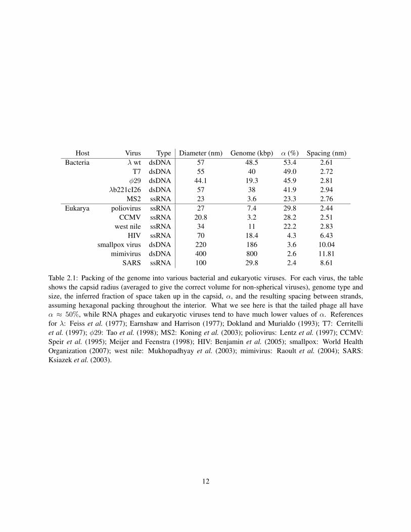
Host Virus Type Diameter (nm) Genome (kbp) α (%) Spacing (nm)Bacteria λ wt dsDNA 57 48.5 53.4 2.61

T7 dsDNA 55 40 49.0 2.72φ29 dsDNA 44.1 19.3 45.9 2.81

λb221cI26 dsDNA 57 38 41.9 2.94MS2 ssRNA 23 3.6 23.3 2.76

Eukarya poliovirus ssRNA 27 7.4 29.8 2.44CCMV ssRNA 20.8 3.2 28.2 2.51

west nile ssRNA 34 11 22.2 2.83HIV ssRNA 70 18.4 4.3 6.43

smallpox virus dsDNA 220 186 3.6 10.04mimivirus dsDNA 400 800 2.6 11.81

SARS ssRNA 100 29.8 2.4 8.61

Table 2.1: Packing of the genome into various bacterial and eukaryotic viruses. For each virus, the tableshows the capsid radius (averaged to give the correct volume for non-spherical viruses), genome type andsize, the inferred fraction of space taken up in the capsid, α, and the resulting spacing between strands,assuming hexagonal packing throughout the interior. What we see here is that the tailed phage all haveα ≈ 50%, while RNA phages and eukaryotic viruses tend to have much lower values of α. Referencesfor λ: Feiss et al. (1977); Earnshaw and Harrison (1977); Dokland and Murialdo (1993); T7: Cerritelliet al. (1997); φ29: Tao et al. (1998); MS2: Koning et al. (2003); poliovirus: Lentz et al. (1997); CCMV:Speir et al. (1995); Meijer and Feenstra (1998); HIV: Benjamin et al. (2005); smallpox: World HealthOrganization (2007); west nile: Mukhopadhyay et al. (2003); mimivirus: Raoult et al. (2004); SARS:Ksiazek et al. (2003).

12

which is the familiar expression for the osmotic pressure Π. We have

ΠNa = ρ · kBT = 2 nm−3 · 4 pN nm = 8.0 pN nm−2 = 79 atm . (2.6)

Alternatively, for Mg2+, we find an osmotic pressure reduced by a factor of two, to 40 atm.

The intent of the preceding estimates is to give us a feeling for the high concentrations and pressures

found within a phage capsid. Strictly, what the partial derivative in Equation 2.5 means is that this pressure

quantifies how Gconf changes if the capsid volume is changed without a concurrent change in the number of

counterions. One way that the volume accessible to counterions can increase is if the DNA is translocated

into the capsid, say by a distance ∆x. The change in accessible volume is given by π r2DNA ·∆x. This means

that we multiply 8.0 pN nm−2 by the cross-sectional area of DNA to find Fconf = 25 pN, an estimate for the

scale of the force that the pressure applies to the DNA at the beginning of genome translocation. However,

as the DNA exits the capsid, the number of counterions within the capsid will change. We must add terms to

Fconf that take into account the change in Gconf with respect to the number of counterions. In the language

of thermodynamics, these terms represent the difference in chemical potential encountered by the ions as

they exit the capsid.

To estimate the force more precisely, we consider a system of N ions, with N1 found in a volume

of water V1 within the capsid, and N2 found in a volume of water V2 outside of the capsid. Following

Equation 2.4, the numbers of arrangements of the ions inside and outside of the capsid are V N11 and V N2

2 ,

respectively. An additional factor(

NN1

)accounts for the number of possible choices for which ions are found

within the capsid, giving us an expression for the total entropy:

S = kB log[(

N

N1

)V N1

1 V N22

]≈ kB log

[NN1

N1N1

V N11 V N2

2

]. (2.7)

We compute the force on the DNA by differentiating the free energy with respect to the length LDNA of the

DNA left inside the capsid:

Fconf = −TdS

dLDNA≈ −kBT

[dN1

dLDNAlog N − dN1

dLDNAlog N1 (2.8)

+dN1

dLDNAlog V1 −

N1

V1· πr2

DNA −dN1

dLDNAlog V2 +

N2

V2· πr2

DNA

],

13

which we can rewrite conveniently as

Fconf = TdS

dLDNA≈ kBT

[dN1

dLDNAlog

ρ1

ρ+ (ρ1 − ρ) · πr2

DNA

], (2.9)

where ρ is the concentration of counterions outside of the capsid and ρ1 is the concentration inside. The

force is positive, i.e., directed out of the capsid, and made up of two terms. The first corresponds to the force

required to transport ions against a chemical potential difference, while the second is the pressure-area force

that we calculated earlier. In terms of the parameters relevant to λ, we have

dN1

dLDNA=

2 e−

qion · 0.34 nm; (2.10)

ρ1 =2 e−LDNA/qion/0.34 nmVcapsid − πr2

DNALDNA. (2.11)

It is apparent that as DNA leaves the capsid, the pressure will decrease. A plot of the quantitative predictions

of this model is shown in Figure 2.4. What we see from this plot is that forces of 100–200 pN are predicted;

the shape of the curve is dominated by the logarithmic chemical potential term. In fact, by completely

ignoring the three-dimensional arrangement of the ions inside and outside the capsid, we are missing some

important details that reduce Fconf to a fraction of this value. Theoretical treatments such as the Poisson-

Boltzmann approximation or the theory of condensation by Manning (1969) would take into account the fact

that some ions remain close to DNA after its exit from the capsid, reducing the entropy gain from exiting

DNA. However, for a variety of reasons, first principles models of the pressure within tightly-packaged DNA

do not give very accurate results when compared to real-world data. Perhaps the most important is the fact

that the discrete nature of the ions is ignored in continuum statistical mechanics approximations. Ion-ion

interactions and the particular locations of the charged phosphate groups on the DNA backbone are both

difficult to model in a simple theory. A Monte Carlo simulation technique by Lyubartsev and Nordenskiold

(1995) was successful in taking these features into account, but the effects of large-scale bending fluctuations

in the structure of DNA itself could not be included.

2.1.3 Simple model II: empirical interstrand forces

Beyond theoretical calculations, the most reliable numbers come from measurements on bulk DNA, com-

pressed by osmotic pressure (Rau et al. 1984; Parsegian et al. 1986; Podgornik et al. 1995; Strey et al. 1997,

1998). These authors used X-ray scattering to measure the osmotic pressure Π required to compress DNA

14

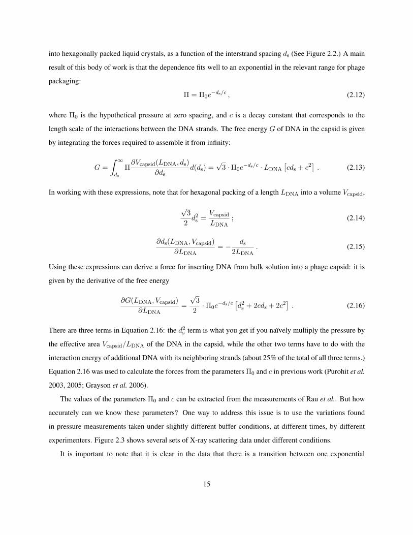
into hexagonally packed liquid crystals, as a function of the interstrand spacing ds (See Figure 2.2.) A main

result of this body of work is that the dependence fits well to an exponential in the relevant range for phage

packaging:

Π = Π0e−ds/c , (2.12)

where Π0 is the hypothetical pressure at zero spacing, and c is a decay constant that corresponds to the

length scale of the interactions between the DNA strands. The free energy G of DNA in the capsid is given

by integrating the forces required to assemble it from infinity:

G =∫ ∞

ds

Π∂Vcapsid(LDNA, ds)

∂dsd(ds) =

√3 ·Π0e

−ds/c · LDNA

[cds + c2

]. (2.13)

In working with these expressions, note that for hexagonal packing of a length LDNA into a volume Vcapsid,

√3

2d2

s =Vcapsid

LDNA; (2.14)

∂ds(LDNA, Vcapsid)∂LDNA

= − ds

2LDNA. (2.15)

Using these expressions can derive a force for inserting DNA from bulk solution into a phage capsid: it is

given by the derivative of the free energy

∂G(LDNA, Vcapsid)∂LDNA

=√

32·Π0e

−ds/c[d2

s + 2cds + 2c2]

. (2.16)

There are three terms in Equation 2.16: the d2s term is what you get if you naıvely multiply the pressure by

the effective area Vcapsid/LDNA of the DNA in the capsid, while the other two terms have to do with the

interaction energy of additional DNA with its neighboring strands (about 25% of the total of all three terms.)

Equation 2.16 was used to calculate the forces from the parameters Π0 and c in previous work (Purohit et al.

2003, 2005; Grayson et al. 2006).

The values of the parameters Π0 and c can be extracted from the measurements of Rau et al.. But how

accurately can we know these parameters? One way to address this issue is to use the variations found

in pressure measurements taken under slightly different buffer conditions, at different times, by different

experimenters. Figure 2.3 shows several sets of X-ray scattering data under different conditions.

It is important to note that it is clear in the data that there is a transition between one exponential

15

dependence and another with a higher value of c. Since the force is derived from an integral over all DNA

spacings, this will have an effect, especially at low packing fractions. Let us define the two exponential

regimes as:

Π =

Π0e

−ds/c if ds < a ;

Π′0e−ds/c′

otherwise.(2.17)

Here we set

Π′0 = Π0e

−a/c+a/c′(2.18)

to ensure that the function is continuous. With this new formula, we can recalculate:

Gconf =

√3 ·Π0e

−ds/c · LDNA

[cds + c2

]−√

3 ·Π0e−a/c · LDNA

[ca + c2

]+√

3 ·Π′0e−a/c′ · LDNA

[c′a + c′2

]if ds < a ;

√3 ·Π′

0e−ds/c′ · LDNA

[c′ds + c′2

]otherwise.

(2.19)

Fconf =

√3

2 ·Π0e−ds/c

[d2

s + 2cds + 2c2]−√

3 ·Π0e−a/c ·

[ca + c2

]+√

3 ·Π′0e−a/c′ ·

[c′a + c′2

]if ds < a ;

√3

2 ·Π′0e−ds/c′

[d2

s + 2c′ds + 2c′2]

otherwise.

(2.20)

Note that the equations imply that Fconf is a continuous function of ds, despite the change in parameters at

ds = a. The value of ds can be found as a function of LDNA and Vcapsid from Equation 2.14. Figure 2.3

shows our fits to the various sources of experimental data on DNA packing, together with predictions from

the present model for λ. What we see is a 30–60% variation of Fconf, depending on the source of the data

used in fitting. This is due to differences in buffer conditions and also probably systematic errors in the

experimental techniques, which differ slightly between the datasets. We have chosen the parameters derived

from the more recent datasets for use in further calculations, including the plot of Fconf shown in Figure 2.4.

2.1.4 Simple model III: only bending energy

So far we have considered the energy required to bring strands of DNA in a closely packed arrangement.

Because Rcapsid is on the same scale as or smaller than ξ, the entire length of the λ genome must be tightly

16

5

5.5

6

6.5

7

7.5

8

8.5

24 26 28 30 32 34 36 38 40

log

10

(P/(

dy

ne/

cm2))

interstrand spacing (A)

Rau 1984 100mM Na dataRau private 50mM Na dataRau 1984 5/25mM Mg dataRau private 10mM Mg data

Condition Π0 (pN/nm2) c (nm) c′ (nm) Fconf (48.5 kbp) (pN) Fconf (38 kbp) (pN) Fconf (24.3 kbp) (pN)Na, 1984 5.9× 103 0.37 0.62 43.1 22.2 9.3Na, 2004 2.1× 104 0.34 0.75 70.7 37.4 16.7Mg, 1984 2.3× 104 0.28 0.35 14.5 5.8 0.9Mg, 2004 1.9× 105 0.23 0.87 20.0 7.5 3.3

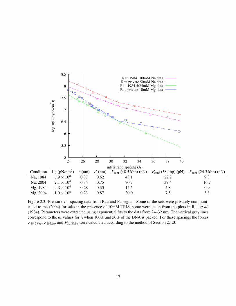
Figure 2.3: Pressure vs. spacing data from Rau and Parsegian. Some of the sets were privately communi-cated to me (2004) for salts in the presence of 10mM TRIS, some were taken from the plots in Rau et al.(1984). Parameters were extracted using exponential fits to the data from 24–32 nm. The vertical gray linescorrespond to the ds values for λ when 100% and 50% of the DNA is packed. For these spacings the forcesF48.5 kbp, F38 kbp, and F24.3 kbp were calculated according to the method of Section 2.1.3.

17

bent to fit into the capsid (Garcia et al. 2007), so there is an additional energy that should be considered: the

bending energy of DNA, which is given in (Boal 2002):

∆Ebend = ∆L · 12ξkBTR−2 , (2.21)

where R is the radius of curvature of a length L of DNA. Let us consider a model in which the capsid is

filled uniformly with a length LDNA of DNA, but only the bending energy contributes to Fconf. Following

Purohit et al. (2003), we will assume that the DNA is packed into an inverse-spool, though a ball-of-twine

model in which the axis of spooling varies with radius could lead to a slightly smaller Fconf (calculation not

shown). For an inverse spool, the total bending energy is given by an integral of Equation 2.21 over the

volume of the capsid, which can be thought of as a sum of many concentric cylindrical shells of DNA of

area 4πr√

R2capsid − r2. We will assume the DNA is packed down to an inner radius of Rin, which gives

the following expression for the total energy:

Ebend =ξkBT

2

∫ Rcapsid

04πr

√R2

capsid − r2r−2 L

Vcapsiddr (2.22)

= 4πξkBTLRcapsid

2Vcapsid·[log

R

Rin+ log

(√1−R2

in/R2capsid

)−

√1−R2

in/R2capsid

](2.23)

≈ ξkBTL

2· (0.33 ·Rcapsid)−2 , (2.24)

where we have obtained the final approximation by putting in a value of 1 nm for Rin, representing the

absolute limit of DNA bending. (The result is very weakly dependent on Rin.) What this expression means

is that DNA has the same bending energy that it would have if it were all bent at an “average” radius of

0.33 ·Rcapsid. This means that DNA feels a force during translocation of

Fconf =dEbend

dL=

ξkBT

2· (0.33 ·Rcapsid)−2 ≈ 1.2 pN . (2.25)

This value is an upper bound for the contribution of DNA bending stiffness to Fconf: according to the inverse

spool model, at low packing fractions the DNA arranges itself around the outer surface of the capsid, with

a higher average radius than for a fully packed capsid, so we would expect the bending force to be lower.

However, as shown in Figure 2.4, the value of 1.2 pN is so low that we don’t expect it to play any important

role.

18

2.1.5 Comparison of the models

Figure 2.4 compares the models derived in the previous three sections. What we can see from this graph is

that the model based on counterion entropy alone (Model 1) gives much higher predictions for Fconf than

the model based on empirical measurements of DNA (Model 2). Most of the difference between these two

models appears during the first 10 kbp of DNA packaging, due to the rising chemical potential difference as

the concentration of ions within in the capsid approaches molar levels. Model 3, taking into account only

the bending energy, predicts a relatively much smaller Fconf, which only exceeds Model 2 when less than

about 10 kbp is packaged. At these low packing fractions, the bending force is actually an overestimate,

since the DNA is able to rearrange, causing Rin to be much larger. More detailed models allow Rin to vary,

effectively combining Models 2 and 3 to compute a energy-minimizing arrangement for the capsid (Purohit

et al. 2003, 2005). However since the contribution of the bending energy to the force is so small, these

models do not predict a significantly different force from Model 2 alone. Model 2 will be used to calculate

Fconf for the remainder of this thesis.

19

0

20

40

60

80

100

120

140

160

0 5 10 15 20 25 30 35 40 45 50

Fo

rce

(pN

)

Packaged DNA (kbp)

Na Buffer

Counterion entropyEmpirical forcesDNA bending

0

10

20

30

40

50

60

70

80

0 5 10 15 20 25 30 35 40 45 50

Fo

rce

(pN

)

Packaged DNA (kbp)

Mg Buffer

Counterion entropyEmpirical forcesDNA bending

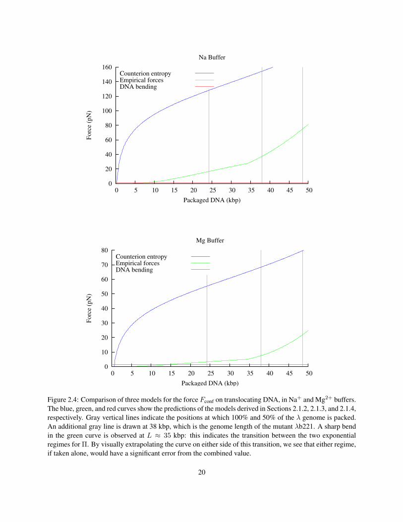
Figure 2.4: Comparison of three models for the force Fconf on translocating DNA, in Na+ and Mg2+ buffers.The blue, green, and red curves show the predictions of the models derived in Sections 2.1.2, 2.1.3, and 2.1.4,respectively. Gray vertical lines indicate the positions at which 100% and 50% of the λ genome is packed.An additional gray line is drawn at 38 kbp, which is the genome length of the mutant λb221. A sharp bendin the green curve is observed at L ≈ 35 kbp: this indicates the transition between the two exponentialregimes for Π. By visually extrapolating the curve on either side of this transition, we see that either regime,if taken alone, would have a significant error from the combined value.

20

2.2 Modeling the mobility of DNA during ejection

Section 2.1 explained how pressure produced by the confined DNA within a phage capsid leads to a force

Fconf during translocation. Other forces may affect translocation: for example a force Fosm originates from

internal osmotic pressure in the host cell. To a student of freshman physics, it is tempting to add up all of

the forces and apply Newton’s law. Suppose the total force is F = 1 pN. Using the mass of the λ genome,

we find the accelerationdv

dt=

F

m=

1 · 10−12 N5 · 10−20 kg

= 2 · 107m/s2 . (2.26)

Clearly such an acceleration can’t continue for very long: like all macromolecular systems, the DNA will

be constrained by molecular-scale friction. Instead of acceleration, we have a force balance:

Fconf + Fosm + Ffric(v) = 0 . (2.27)

It is not clear how to address friction at the molecular level. However, since the DNA is in a fluid state (Strey

et al. 1997), we expect the frictional force Ffric(v) to behave like macroscopic hydrodynamic drag, increas-

ing with velocity. In fact, it will be useful to assume a linear dependence:

Fconf + Fosm − v/µ = 0 , (2.28)

where µ, which we call the mobility, characterizes the frictional force. The problem of modeling friction

during DNA ejection is that µ depend on the configuration of the DNA. With one exception (Zarybnicky

1969), theoretical papers have avoided explicitly estimating the friction, focusing instead how the friction

should scale with parameters like the concentration of DNA within the capsid (Gabashvili and Grosberg

1991, 1992; Spakowitz and Wang 2005; Inamdar et al. 2006). However, Section 3.2 describes an experiment

that can make a direct measurement of µ, demanding a theoretical interpretation. This section aims to satisfy

that demand with several quantitative estimates of µ.

2.2.1 Friction in the phage tail

In this section we discuss the drag that is experienced by the DNA as it translocates through the tail, due to

friction in a hypothetical layer of water between the DNA and the inner wall of the tail. The method of this

section was essentially described by Zarybnicky (1969).

21

We begin by assuming that the pore opened by the phage is a annular tube: it is bounded by the DNA

on the inside and the tail proteins on the outside. The general solution for cylindrically symmetric flow with

an inner boundary at rDNA is a standard result; see, for example, Weisstein (2005). The flow velocity u is a

function only of r, given by:

u(r) = u(rDNA)− Q

4ηLtail

(r2 − r2

DNA − c log(r/rDNA))

. (2.29)

Here Q represents the pressure difference along the length of the tail. In the case of DNA translocation at

velocity v, the boundary conditions are that u(rDNA) = v and u(Rtail) = 0, resulting in a value for the

constant c of:

c =R2

tail − r2DNA − v · 4ηLtail

Q

log Rtail/rDNA. (2.30)

The shear force exerted by the water on the DNA is given by

Ftail = 2πrDNALtailηdu

dr= −πrDNA

Q

2(2rDNA − c/rDNA) . (2.31)

Substituting the value of c from Equation 2.30 and expanding the result, we find

Ftail = −πrDNAQ

2

(2rDNA −

R2tail − r2

DNA

rDNA log Rtail/rDNA

)− v · 2πηLtail

log Rtail/rDNA. (2.32)

Notice that Equation 2.32 consists of two terms: one that is linear in the pressure difference Q and one that

is linear in v. Using the values given earlier for η, Rtail, rDNA, and Ltail, we find

Ftail = 3.7 nm2 ·Q− 2.2× 10−4 pN · skbp

· v . (2.33)

We will examine the meaning of Q in Section 2.3; for now, let us assume that Q = 0. Under the assumption

that the tail provides the only source of friction, we find

µ = 4500kbp

s · pN. (2.34)

What should be recognized in this case is that µ is independent of the configuration of the DNA: it will be a

constant throughout the translocation process. Also, it should be understood that under this approximation,

pN-scale forces will be sufficient to complete translocation within 10 ms. This value of µ is compared to

22

other predictions for the mobility in Figure 2.5.

2.2.2 Friction in the phage head

Gabashvili and Grosberg (1991) suggested three sources of friction for genome translocation: friction in

the tail, friction between the DNA and the inner surface of the phage head, and friction between neighbor-

ing sections of DNA in the head. Section 2.2.1 focused on the first source of friction; in this section we

will make an estimate of the last, which is caused by DNA sliding past itself as it exits the capsid. In a

hexagonally-packed arrangement, one section of the DNA has six neighbors, separated from it by a water

layer of thickness ds − 2 · rDNA. As the DNA slides out of the capsid, each of the neighbor sections will

be moving, possibly in different directions. The central section will be subjected to a friction that depends

on how fast the neighbors move: if they move in opposition, the force will slow down translocation, while

if they move together, the force will speed up translocation. We have no way of knowing what the exact

arrangement of the DNA will be as it slides out, so we suggest a reasonable approximation: assume that the

opposing and aligned motions of the neighbor strands cancel out to an average of zero velocity. Then we

can imagine that the central strand is actually moving within a stationary tube of radius ds − rDNA, so the

force can be found with Equation 2.32:

Fhead = − v · 2πηLDNA

log (ds − rDNA)/rDNA; (2.35)

µ =1

2πηLDNA· log

ds − rDNA

rDNA. (2.36)

Here, LDNA is the amount of DNA remaining in the capsid. According to Table 2.1.2, for a fully packed λ

(LDNA = 16µm) we have ds = 2.61 nm. These numbers lead to the numerical result

µ = 6.8 µm · s−1 pN−1 = 20. kbp · s−1 pN−1 . (2.37)

The friction is about 200 times stronger under this approximation, which makes sense, since the genome

is about 200 times longer than the tail alone. However, as the DNA exits the capsid, LDNA will decrease,

causing µ to increase. The predictions of a mobility model, taking into account only the friction in head, are

plotted in Figure 2.5.

23

2.2.3 Friction from layer sticking (Grosberg/Rubinstein model)

This section discusses an idea proposed by Rubinstein and Grosberg (2007) to explain experimental mea-

surements of mobility by Grayson et al. (2007) (we discuss the experiments in Section 3.2.) The basic result

of those experiments is that µ is an exponential function of the amount of DNA within the capsid with a

decay constant of L0 ≈ 10 kbp. The suggestion, based purely on the empirical observation of an expo-

nential dependence, is that this could be modeled by hypothetical stickers on the DNA, spaced at a linear

density σ on the DNA, that fluctuate between bound and unbound states. When bound, the DNA is “stuck”

and unable to translocate, but when the sticker is unbound, it may translocate freely. Suppose that when it

is moving freely in the head, it has mobility µ0 = 4500 kbp/s · pN given entirely by resistance in the tail.

To understand the implications of this model, we must compute how much time the DNA spends in its free

state.

We model the stickers with the assumption that each has a probability of being unbound given by the

Boltzmann factor:

P1 =exp(−ε/kBT )

1 + exp(−ε/kBT ), (2.38)

where ε is the sticking energy. Then the probability for the N = σL stickers to all be simultaneously

unbound, allowing the DNA to move, is

P =(

exp(−ε/kBT )1 + exp(−ε/kBT )

)σL

. (2.39)

Then the average mobility is given by

µ = µ0 ·(

exp(−ε/kBT )1 + exp(−ε/kBT )

)σL

. (2.40)

Since ε and σ are unknown and probably unmeasurable constants, it will be most useful to rewrite this in a

simpler form:

µ = µ0 · exp(−L/L0) , with (2.41)

L0 = −σ−1 log(

exp(−ε/kBT )1 + exp(−ε/kBT )

). (2.42)

Note that since the factor within the log is P1, which is always less than one, it is not possible for L0 to

24

equal σ−1 under any circumstances. In fact, for the likely situation that ε > kBT , we have

L0 = σ−1ε/kBT . (2.43)

Suppose, for example, sticking corresponds to a typical hydrogen bonding interaction with ε/kBT ≈ 10.

Then we have

σ−1 = L0/10 ≈ 1 kbp . (2.44)

It is not clear what process could cause sticking every 1 kbp. The outer loops of DNA that make contact

with the capsid have sizes of approximately 300 bp, while an entire layer of DNA loops in the inverse spool

model contains about 5–10 kbp.

Alternatively, suppose that every base pair is equally likely to cause sticking:

σ−1 = 1 bp ; (2.45)

ε/kBT = 10−4 . (2.46)

In this case, for the sticking model to be correct, we would have to think of a mechanism by which bases

can cause sticking with a probability of approximately 10−4. The usefulness of this model is limited by our

inability to think of a physical mechanism for the sticking process. In fact, since the model was just created

as an explanation for the data, we have no particular reason to believe that it accurately represents the reality

of the motion of the phage DNA. For example, it may be that a single loop or layer of DNA may move

without it being necessary for the entire length of the genome to be sliding; these possibilities may or may

not lead to different functional forms for µ. Despite the limitations of this model, its predictions are plotted

for in Figure 2.5.

25

10

100

1000

10000

100000

0 10 20 30 40 50

Mo

bil

ity

(k

bp

/s/p

N)

Packaged DNA (kbp)

Tail modelHead model

Sticker model

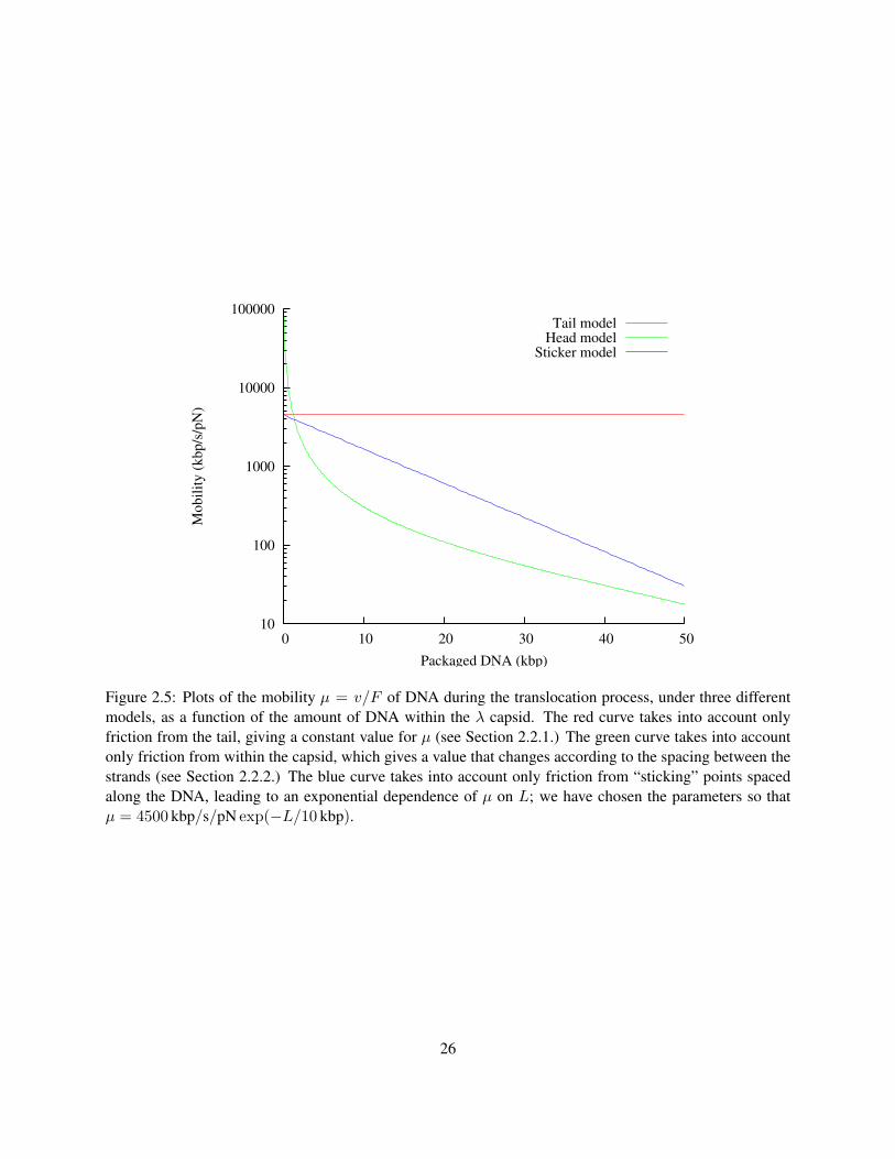
Figure 2.5: Plots of the mobility µ = v/F of DNA during the translocation process, under three differentmodels, as a function of the amount of DNA within the λ capsid. The red curve takes into account onlyfriction from the tail, giving a constant value for µ (see Section 2.2.1.) The green curve takes into accountonly friction from within the capsid, which gives a value that changes according to the spacing between thestrands (see Section 2.2.2.) The blue curve takes into account only friction from “sticking” points spacedalong the DNA, leading to an exponential dependence of µ on L; we have chosen the parameters so thatµ = 4500 kbp/s/pN exp(−L/10 kbp).

26

2.3 Calculating drag forces in the toilet-flush model

In the preceding sections we have discussed a theoretical model of the pressure within the capsid as well as

the friction that may be encountered during DNA translocation. It is also essential to consider the kinds of

forces that may be encountered when λ is actually ejecting its DNA into a host cell, since the phage/host

interaction may play an important role. Some discussion about the various kinds of effects that may come

into play during DNA translocation in vivo is given in Section 3.3. Here we will describe the details of one

source of force that may speed up DNA translocation. The model described in this section is also described

elsewhere (Grayson and Molineux 2007).

2.3.1 Precise definition of osmotic pressure

Because bacterial cells lack a cytoskeleton, they rely on an internal pressure to push the cell membrane

outward. This pressure serves both to help maintain the cell shape and to allow the cytoplasm to increase in

volume as the cell grows. The internal pressure is created by the presence of concentrated solutes within the

cytoplasm, though it is unclear which solutes play the dominant role. Solutes by definition have an affinity

for water, so that there is an free-energy decrease associated with transferring a small volume ∆Vwater of

water into the cell,

∆Fosm = −Π ·∆Vwater , (2.47)

where Π is the cytoplasmic osmotic pressure, a number that depends on the concentrations of various solutes

in the cytoplasm relative to the extracellular space. This osmotic pressure can be measured in various ways:

Stock et al. (1977) measured the cellular contents of E. coli under various osmotic conditions and computed

a theoretical pressure of 0.33 pN/nm2 for E. coli growing rapidly but approaching saturation; Knaysi (1951)

applied plasmolysis, a contraction of the cytoplasm away from the outer membrane, at various times during

growth of an E. coli culture, finding an osmotic pressure up to 1.5 pN/nm2 during initial rapid growth,

which stabilized at 0.2 pN/nm2. More references and discussion about the osmotic pressure within E. coli

can be found in Neidhardt (1996), p. 1211. We will take Π = 0.3 pN/nm2, or 3 atm as a standard value.

In the absence of any constraints, water will flow into the cytoplasm, diluting the internal solutes, until the

Π = 0; the cytoplasm will then be in equilibrium with the extracellular space. However, if the cell volume

is constrained by a rigid cell membrane, the transfer of water results in an increase of internal hydrostatic

27

pressure, defined by a free energy cost

∆Fhyd = P ·∆Vwater . (2.48)

In this case, water will continue to flow into the cell until an equilibrium is reached where the net free energy

benefit of transferring water is zero; where

P = Π . (2.49)

In many situations, this equilibrium is reached quickly, so there is no need to make a distinction between

osmotic pressure and the resulting hydrostatic pressure.

However, during rapid cell growth, the cytoplasm is clearly out of equilibrium to some extent, since

water is continuously flowing into the cell. In addition, there are various experimental techniques that

involve subjecting a cell to osmotic shocks, causing the cytoplasm to shrink or swell; in these experiments,

the cell is therefore temporarily out of equilibrium. The remainder of this section is concerned with the

problem of quantifying the extent to which the cell is out of equilibrium under these different conditions.

In particular, we will try to quantify the pressure imbalance Q ≡ Π − P , which will be positive whenever

water is flowing into the cell, and negative when water is flowing out.

For the following estimates we will assume that E. coli has a cell volume of 0.4 µm3 = 4 × 108nm3.

During rapid growth, E. coli divides once every 1200 s. This means that water must flow into the cell at a

rate of

Φ = 4× 108 nm3/1200 s = 3.3× 105 nm3/s . (2.50)

The pressure imbalance depends on the permeability of the cytoplasmic membrane to water: a more

permeable membrane will allow the cell to stay closer to equilibrium. To estimate this permeability, we

turn to experiments in which measured osmotic shocks cause measurable changes in cytoplasmic volume.

Delamarche et al. (1999) report a water channel, AqpZ, that is present in the cytoplasmic membrane of

E. coli. In their experiments, cells are subjected to hyperosmotic shocks (Q < 0), causing a shrinkage of the

cytoplasm, observable under cryo-electron microscopy, known as plasmolysis. From their graphs we see that

a 1 osM (2.6 pN/nm2) shock causes AqpZ+ cells to begin shrinking at a rate of ∼0.2 cell volumes/15 s =

5.3× 106 nm3/s, while AqpZ- cells shrink much more slowly, at about 6.7× 105 nm3/s. From this we can

infer that AqpZ is the primary water device for water transport across the cytoplasmic membrane, and we

can estimate the rate of water flow as a function of pressure. We will assume a linear relationship between

28

the influx Φ of water and Q:

Φ =Q

2.6pN/nm2· 5.3× 106 nm3/s = Q · 2.1× 106 nm3/s · nm2/pN . (2.51)

The coefficient multiplying Q on the right side of Equation 2.51 is the permeability of the cell membrane

to water; the assumption of linearity allows us to make estimates for other conditions. For example, during

rapid growth, the rate of water influx implies a pressure imbalance of

Q = 3.3× 105 nm3/s ·(2.1× 106 nm3/s · nm2/pN

)−1 = 0.16 pN/nm2 . (2.52)

Is the cell permeability given in Equation 2.51 reasonable? A simple hydrodynamics calculation shows

that it is. Laminar fluid flow through a cylindrical pipe is traditionally calculated using a formula owed to

Poiseuille:

Φ =Q

l

π

8ηr4 = Q · 1.4× 104 nm3/s , (2.53)

using l = 2 nm and r = 0.15 nm as the length and radius of the AqpZ pore. This would imply that about

150 copies of AqpZ are required to give the cytoplasmic membrane the permeability given in Equation 2.51,

which is a very reasonable number for a membrane channel.

2.3.2 Implications of the toilet-flush model

The key result of the previous section is that the osmotic pressure imbalance Q of E. coli causes an influx

of water through all open channels. As we assumed already in Section 2.2.1, when λ binds to E. coli it also

opens a channel through which water can flow: the space between the DNA and the inner surface of the tail.

This inrush of water will apply a force to the DNA, speeding up translocation into the cell.

Our goal is to compute the rate v at which DNA is translocated into the cytoplasm, in units of kbp/s, as

a function of the amount of DNA that has been translocated. The value of v can be compared to experiments

that quantitatively measure the translocation process. The basic equation that we will use to determine the

dynamics of the system is a balance of forces:

Fconf + Fosm + Ftail(v) = 0 , (2.54)

where Fconf and Fosm are the internal force due to DNA confinement and the cytoplasmic osmotic force,

29

respectively. The function Ftail(v) is the force due to water flowing between the tail and DNA. We have

shown in Section 2.2.1 that Ftail reduces to a linear function of the pressure difference Q and v:

Fconf + Fosm + 3.7 nm2 ·Q− 2.2× 10−4 pN · skbp

· v = 0 . (2.55)

Using the value of Q from Equation 2.52, we get a value of 0.59 pN for the pressure-dependent term of

Ftail. For the value Π = 0.3 pN/nm2 that was quoted earlier, we find that P = 0.14 pN/nm2, much reduced

from its equilibrium value. This allows us to estimate Fosm = P · πr2DNA = −0.44 pN. The force balance

of Equation 2.33 now becomes

v =Fconf + 0.15 pN

2.2× 10−4 pN · s/kbp= Fconf · 4500

kbppN · s

+ 680 kbp/s . (2.56)

This model predicts extremely high velocities for DNA translocation into E. coli, suggesting that the DNA

may be completely translocated into the cell in less that 0.1 s. However, we have made numerous assump-

tions in our calculations, so that our numbers can easily be off by an order of magnitude. For example, the

thickness of the gap between the DNA and tail is not accurately known, and it varies along the length of the

tail. A gap of 0.3 nm, for example, enough for just one layer of water, would result in a prediction that the

term of Ftail depending on Q is not high enough to overcome Fosm; in this case additional source of energy

would be required for translocation of the entire genome. We have also completely ignored the fact that

water itself is discrete on the nanometer scale, so that describing its flow with a continuum fluid dynamics

model is somewhat absurd. However, in the absence of better experimental data on the flow through phage-

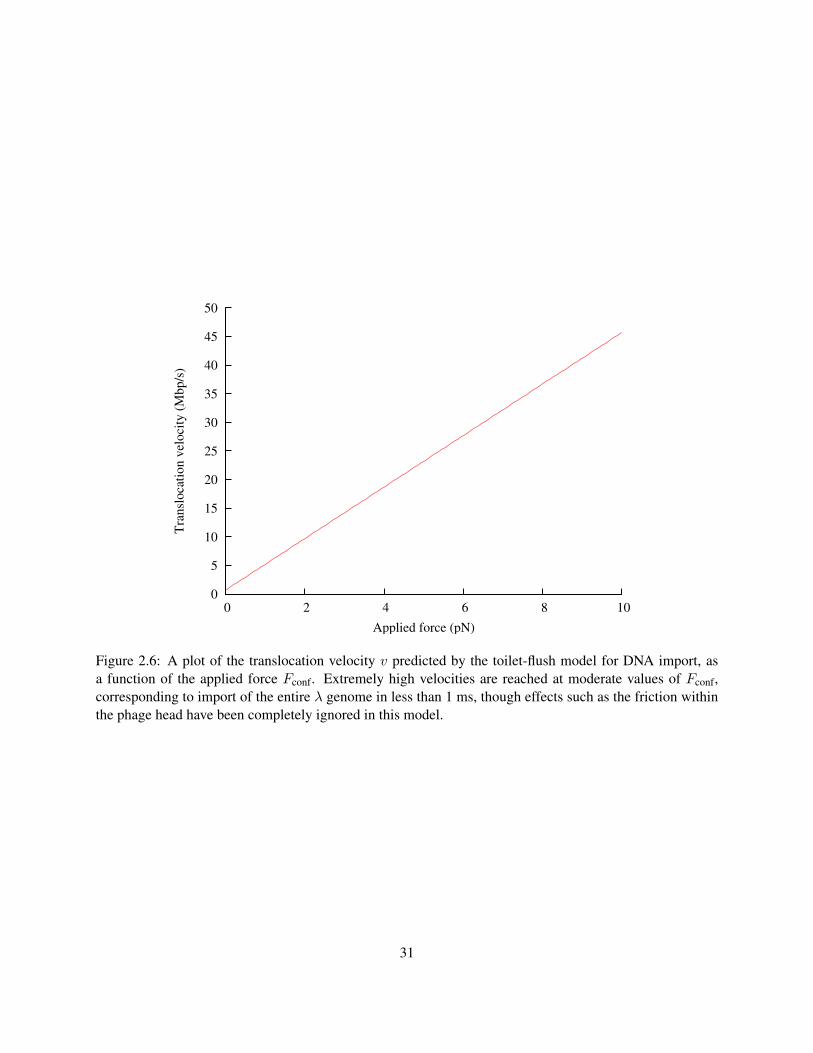
induced channels, the continuum approximation is the best that we have. Figure 2.6 shows the translocation

velocities predicted by this model for forces in the range of 0–10 pN.

The translocation speed at Fconf = 0, 680 kbp/s is fast enough to be consistent with all experiments

on phage ejection in vivo: no phage has ever been observed to eject its DNA faster than that. There are

cases, such as T7, in which the DNA is observed to enter the cell much more slowly; this can be attributed

to mechanisms that slow down the motion of the DNA, such as a constriction region in the channel causing

direct channel-DNA interaction (Kemp et al. 2004).

The only source we used for the permeability of cell membranes is the study by Delamarche et al. (1999).

A further study, using real-time fluorescence and light scattering measurements, concluded that plasmolysis

can occur approximately 500 times faster, implying a much more permeable cell membrane (Hubert et al.

30

0

5

10

15

20

25

30

35

40

45

50

0 2 4 6 8 10

Tra

nsl

oca

tio

n v

elo

city

(M

bp

/s)

Applied force (pN)

Figure 2.6: A plot of the translocation velocity v predicted by the toilet-flush model for DNA import, asa function of the applied force Fconf. Extremely high velocities are reached at moderate values of Fconf,corresponding to import of the entire λ genome in less than 1 ms, though effects such as the friction withinthe phage head have been completely ignored in this model.

31

2005). It is unclear why there is such a huge discrepancy between the two results, but such a highly perme-

able cell membrane would make the forces computed in this paper entirely negligible. The former paper is

more satisfying, both because of its single-cell images that reveal exactly what is happening in the experi-

ment, and because it provides a natural explanation for why bacterial cells must be highly pressurized. It is

also worth mentioning that, according to our calculations, the AqpZ- mutants of Delamarche et al. (1999)

should not be able to grow as rapidly as the wild-type, unless they have an internal osmotic pressure of at

least 1.6 pN/nm2 = 16 atm.

We assumed 0.3 pN/nm2 for the osmotic pressure inside of a cell without much comment, but, as was

discussed, it may be five times higher during rapid growth, presenting a much higher force resisting DNA

entry.

To conclude, we have thoroughly considered the motion of water molecules entering the cytoplasm

through a phage-induced channel. It appears that forces from hydrodynamic drag may be a significant

contributor to the total force on the DNA, and that they are potentially responsible for translocation of the

entire genome. In estimating these forces, it is essential to understand the difference between hydrostatic and

osmotic pressures, which will not be equal in non-equilibrium situations. In any case, there are numerous

unknown quantities in the estimates, and it is hard to draw strong conclusions about the role of hydrodynamic

drag. Experiments to examine these hydrodynamic forces, and non-equilibrium osmotic pressure in general,

would be of much use in clarifying these issues.

32

Chapter 3

Experiments on the bacteriophage ejectionprocess

It is the author’s strong belief that for biology, theory and experiment must go together. A good theory

makes predictions for quantities that can be tested experimentally, which is why Chapter 2 makes a series

of specific predictions, without any free parameters. Even when the parameters are unknown, it is important

to make reasonable estimates, so that it is possible to identify theories that make completely unreasonable

predictions. Similarly, it is essential for experimenters to design experiments to give quantitative results that

can be directly compared to theory. In this chapter we describe a series of experiments on λ that complement

the theoretical models. With the model set by Luria and Delbruck in mind, we hope that for some of the cases

agreement between theory and experiment will clarify our understanding of how phages work. Specifically,

we have carried out an experiment (Section 3.1) to test the pressure estimates of Section 2.1; an experiment

(Section 3.2) that measures the velocity of DNA ejection from λ in vitro, for comparison to the estimates

of mobility in Section 2.2; and we have made progress on an experiment to visualize the ejection process

in vivo (Section 3.3) for comparison to models such as the one presented in Section 2.3. In Section 3.4,

we discuss a comparison of our results on the ejection process with measurements on DNA packaging in

phages.

3.1 Experimental measurement of ejection force

An experimental measurement of the internal force Fconf (defined in Section 2.1) driving ejection of DNA

from λ capsids has been published (Grayson et al. 2006). The goal was to measure Fconf as a function of

the amount of DNA within the capsid, using the procedure of Evilevitch et al. (2003), with modifications to

33

Figure 3.1: Experimental measurement of ejection force. A. LamB binds to phage tails, triggering theejection of DNA. The ejection reaches an equilibrium when the internal force balances the osmotic force dueto PEG. B. DNase I cuts the ejected DNA into small fragments. C. Phages are removed by centrifugation,leaving the ejected fraction of the DNA in solution. See Section C.7 for the details of the procedure.

bring the accuracy to the level where the quantitative theory of Section 2.1 may be tested. Most generally,

the model predicts that Fconf is a function only of the amount of DNA within the capsid; what this means

is that the original genome size of the phage should not affect Fconf. A fortuitous feature of λ is that there

are mutants available with different genome sizes: in this experiment, we used λcI60, which has a wild-type

genome length of 48.5 kbp, and λb221cI26, with a genome length of approximately 38 kbp (Feiss et al.

1977). See Section C.3 for the technique we used to accurately measure the length of λ genomes.

The experimental procedure is described in detail in Section C.7 and is illustrated in Figure 3.1. Essen-

tially, 200 µL samples were prepared containing phages, an excess of purified LamB, the DNA-digesting

34

enzyme DNase I, and polyethylene glycol (PEG) at a known concentration. The phages bound to LamB, re-

leasing their DNA into the medium. Without PEG, the entire genome is released due to the force from its in-

ternal pressure. With PEG, an external osmotic pressure is present that applies a resisting force to the DNA,

preventing it from escaping completely. The osmotic pressure is given by the empirical formula (Michel

1983):

Π(atm) = −1.29G2T + 140G2 + 4G ; (3.1)

G ≡ w/(100− w) , (3.2)

where T is the temperature (unitless, representing ◦C) and w is the %(w/w) weight-weight fraction of PEG,

w = mPEG/mtot. It is important to note that Π is an increasing function of w and a decreasing function

of T . This experiment is conducted entirely at T = 37. To take into account the excluded volume in the

PEG-DNA interaction, we estimate the osmotic force on the DNA as

Fosm = Π · π(rDNA + rPEG)2 , (3.3)

where rPEG = 0.2 nm is chosen to represent half of the experimentally determined PEG monomer length (Ab-

bot et al. 1992; Marsh 2004). DNA translocation will proceed until Fosm = Fconf. DNase is used to separate

ejected DNA from the capsid: after this equilibrium is reached, centrifugation separates the capsids from

the digested nucleotides. A UV absorbance reading then allows us to find out how much DNA was ejected.

3.1.1 Results

The absorbance spectra for a typical set of data is shown in Figure 3.2. We are interested in the DNA

absorbance peak at 260 nm, and from the figure it is clear that there is a significant shift in this peak due to

absorbance of the cuvette and buffer—the background absorbance. The background depends significantly

on the concentration of PEG, so it is important to measure it separately for each concentration. The third

and fourth rows of Figure 3.2 show the absorbance spectra after the background is subtracted, causing the

260 nm peak to become clearly defined. However, some of the curves are still displaced up or down due to

uncontrollable factors such as imperfections in the cuvette; empirically we identified occasional shifts up or

down of about 0.1 absorbance units in individual spectra. To account for these shifts, all curves were aligned

according to their values at 300 nm; the resulting spectra are directly compared in Figure 3.3.

35

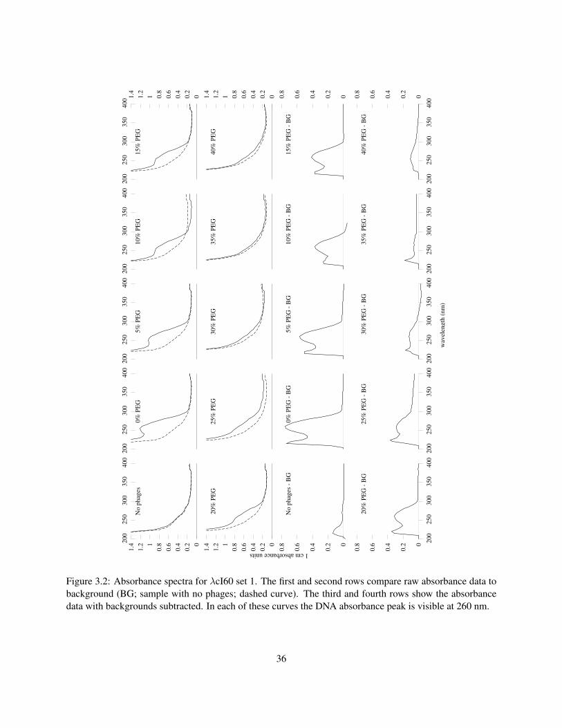
1 cm absorbance units

wav

elen

gth

(n

m)

0

0.2

0.4

0.6

0.8 1

1.2

1.4 2

00

25

0 3

00

35

0 4

00

No

ph

ages

20

0 2

50

30

0 3

50

40

0

0%

PE

G

20

0 2

50

30

0 3

50

40

0

5%

PE

G

20

0 2

50

30

0 3

50

40

0

10

% P

EG

0 0.2

0.4

0.6

0.8

1 1.2

1.4

20

0 2

50

30

0 3

50

40

0

15

% P

EG

0

0.2

0.4

0.6

0.8 1

1.2

1.4

20

% P

EG

25

% P

EG

30

% P

EG

35

% P

EG

0 0.2

0.4

0.6

0.8

1 1.2

1.4

40

% P

EG

0

0.2

0.4

0.6

0.8

No

ph

ages

- B

G

0

% P

EG

- B

G

5

% P

EG

- B

G

1

0%

PE

G -

BG

0 0.2

0.4

0.6

0.8

15

% P

EG

- B

G

0

0.2

0.4

0.6

0.8

20

0 2

50

30

0 3

50

40

0

20

% P

EG

- B

G

20

0 2

50

30

0 3

50

40

0

25

% P

EG

- B

G

20

0 2

50

30

0 3

50

40

0

30

% P

EG

- B

G

20

0 2

50

30

0 3

50

40

0

35

% P

EG

- B

G

20

0 2

50

30

0 3

50

40

0 0 0.2

0.4

0.6

0.8

40

% P

EG

- B

G

Figure 3.2: Absorbance spectra for λcI60 set 1. The first and second rows compare raw absorbance data tobackground (BG; sample with no phages; dashed curve). The third and fourth rows show the absorbancedata with backgrounds subtracted. In each of these curves the DNA absorbance peak is visible at 260 nm.

36

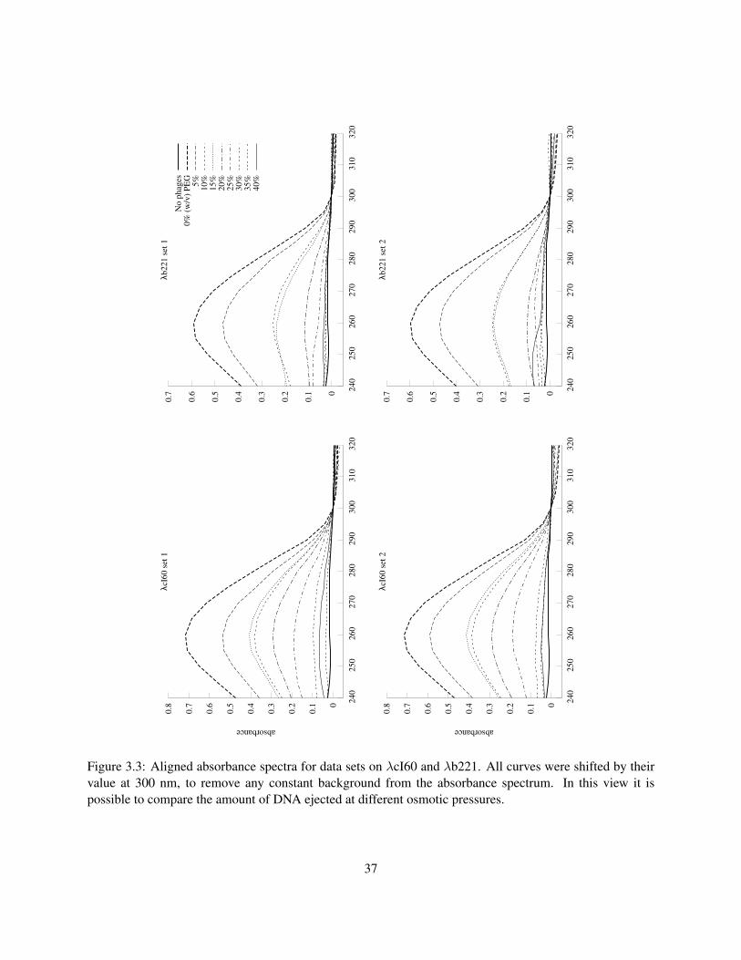
0

0.1

0.2

0.3

0.4

0.5

0.6

0.7

24

0 2

50

26

0 2

70

28

0 2

90

30

0 3

10

32

0

λb2

21

set

1

No

ph

ages

0%

(w

/v)

PE

G5

%1

0%

15

%2

0%

25

%3

0%

35

%4

0%

0

0.1

0.2

0.3

0.4

0.5

0.6

0.7

0.8

24

0 2

50

26

0 2

70

28

0 2

90

30

0 3

10

32

0

absorbance

λcI6

0 s

et 1

0

0.1

0.2

0.3

0.4

0.5

0.6

0.7

24

0 2

50

26

0 2

70

28

0 2

90

30

0 3

10

32

0

λb2

21

set

2

0

0.1

0.2

0.3

0.4

0.5

0.6

0.7

0.8

24

0 2

50

26

0 2

70

28

0 2

90

30

0 3

10

32

0

absorbance

λcI6

0 s

et 2

Figure 3.3: Aligned absorbance spectra for data sets on λcI60 and λb221. All curves were shifted by theirvalue at 300 nm, to remove any constant background from the absorbance spectrum. In this view it ispossible to compare the amount of DNA ejected at different osmotic pressures.

37

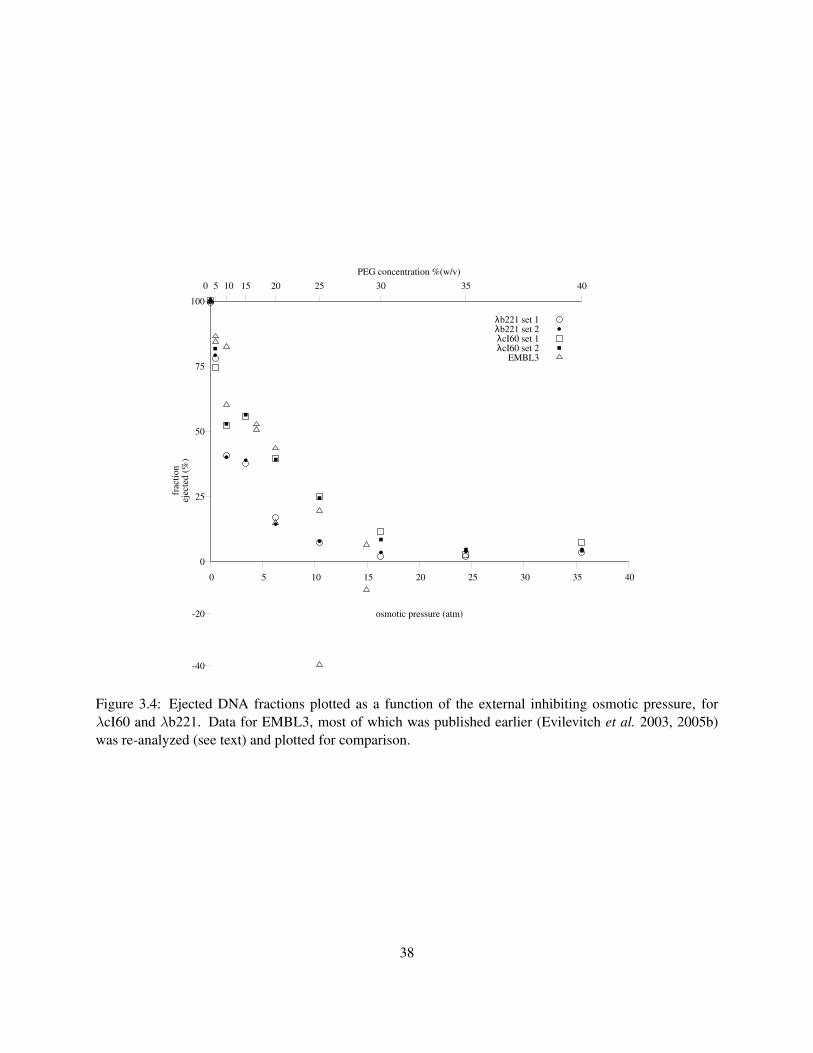
100

75

50

25

0

-20

-40

40 35 30 25 20 15 10 5 0

403530252015

frac

tio

nej

ecte

d (

%)

PEG concentration %(w/v)

0 5 10

osmotic pressure (atm)

λb221 set 1λb221 set 2λcI60 set 1λcI60 set 2

EMBL3

Figure 3.4: Ejected DNA fractions plotted as a function of the external inhibiting osmotic pressure, forλcI60 and λb221. Data for EMBL3, most of which was published earlier (Evilevitch et al. 2003, 2005b)was re-analyzed (see text) and plotted for comparison.

38

After these adjustments, the height of the peaks was considered to be linearly related to the amount of

DNA ejected from the capsid. When there is no PEG in the buffer, 100% of the DNA is ejected (Evilevitch

et al. 2005a), and when no phages are present, no DNA is ejected. Therefore, we can compute the fraction

of DNA that was ejected according to the following interpolation:

ejected fraction = 100% ·A260,with PEG −A260,no phages

A260,no PEG −A260,no phages. (3.4)

The ejected fraction is plotted in Figure 3.4. In this figure, we see that with increasing pressure, the amount

of ejected DNA decreases, as expected based on the above argument about force balance. At all pressures

the ejected fraction for λcI60 was larger than for λb221; this is consistent with the theory that λb221 should

have a lower pressure.

Interestingly, the ejected fraction was almost constant or possibly slightly increasing for both phages be-

tween 1.5 and 3.3 atm: this bump in the data appeared in all datasets taken on several preparations of phages

using equipment at both UCLA and Caltech (not shown), so we are sure that it is a real phenomenon and not

experimental noise. Careful examination of the ejected fraction using finer divisions in PEG concentration

reveals what appears to be a smooth rise followed by a fall, but the origin of this feature is unknown (Koehler

and Phillips 2005). Theoretically, a flat segment of the graph suggests a transition between two states of the

system, for example different geometrical arrangements of the DNA within the capsid. However, in the

absence of more data, we will not be able to suggest any specific theoretical explanation. In particular, the

sharp kink in the theoretical ejection force does not correspond to this feature.

Figure 3.5 shows a different way of looking at the data: by subtracting the amount of ejected DNA from

the genome length, we can derive the amount of DNA remaining in the capsid. In this view, any model of

the DNA within the capsid predicts that the datapoints will all fall on a single curve until the full genome

length is reached, and this is in fact what the figure shows. It is also compared to the theory of Section 2.1.3,

using the approximate relation of Equation 3.3. The theoretical curve falls close to the data, predicting a

force that is always within a factor of two of the measurements.

3.1.2 Error analysis

Errors in the measurements resulted from several sources, each of which was tested. We are only con-

cerned about getting errors right within about 50%, so, since 1mg ≈ 1µL, we can use mg and µL units

interchangeably.

39

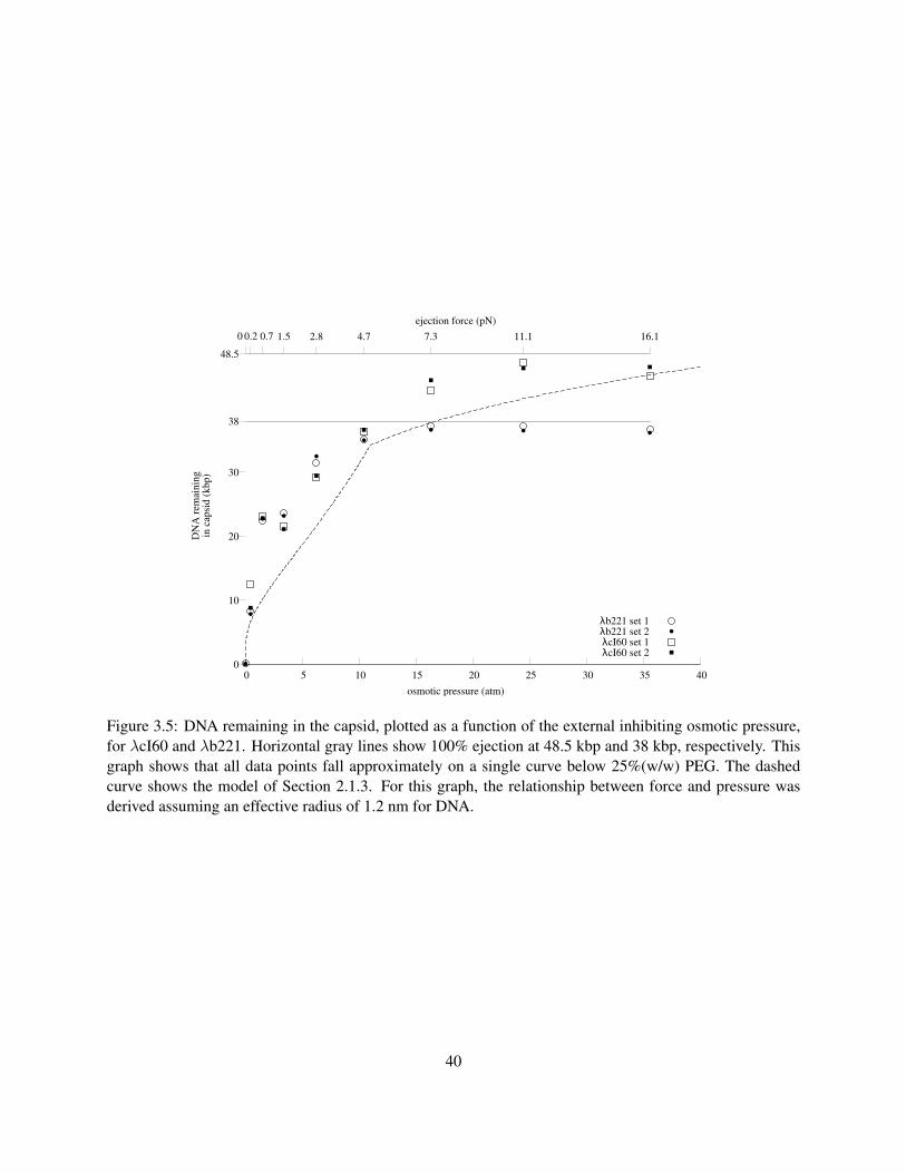
48.5

38

30

20

10

0 40 35 30 25 20 15 10 5 0

16.111.17.34.72.81.5

DN

A r

emai

nin

gin

cap

sid

(k

bp

)

osmotic pressure (atm)

ejection force (pN)

0 0.2 0.7

λb221 set 1λb221 set 2λcI60 set 1λcI60 set 2

Figure 3.5: DNA remaining in the capsid, plotted as a function of the external inhibiting osmotic pressure,for λcI60 and λb221. Horizontal gray lines show 100% ejection at 48.5 kbp and 38 kbp, respectively. Thisgraph shows that all data points fall approximately on a single curve below 25%(w/w) PEG. The dashedcurve shows the model of Section 2.1.3. For this graph, the relationship between force and pressure wasderived assuming an effective radius of 1.2 nm for DNA.

40

• Weighing PEG. This is the first weighing step; each tube was carefully weighed within 0.3 mg:

σPEG = 0.3 µL.

• Weighing TM. As a second step, this is more difficult, so the error is set at 0.4 mg: σTM = 0.4 µL.

• Pipetting LamB. This is done with a wide-mouth tip, so it is the largest source of pipetting error. For

pipetting 10 µL of LamB, a 5% error is estimated: σLamB = 0.5 µL.

• The spectrophotometer, when used with plastic cuvettes, has an error that we measured at 0.007; be-

tween one measurement and another, the absorbance values that we measure vary by about that much.

But to calculate an ejected fraction we multiply the spectrophotometer reading by our calibration, so

we have an error in the measured percentage of

σspec = 100% · 0.007abs100% − abs0%

. (3.5)

• Pipetting λ is done with a narrow tip. It has been estimated from tests of repeated pipetting that

this can be done with a precision of about 2%, resulting in a 2% error in the final measured ejection

percentage. We write this is

σλ = 0.02 · (measured ejection %) . (3.6)

From these numbers we can compute an error in the total volume of the sample. Since the total volume

is a sum of all of the volumes added together, the errors add as follows:

σtot =(σ2

PEG + σ2TM + σ2

LamB) 1

2 = 0.7 . (3.7)

The x-error is the error in osmotic pressure due to an error in PEG concentration. Since the PEG weight

fraction is given by

φPEG = mPEG/vtot , (3.8)

the error in this quantity is

σφPEG = φPEG

{(σPEG

mPEG

)2

+(

σtot

vtot

)2} 1

2

, (3.9)

41

and we get the error in osmotic pressure from the dependence of pressure on PEG concentration:

σx = σΠ =dΠdφ

· φPEG

{(σPEG

mPEG

)2

+(

σtot

vtot

)2} 1

2

=dΠdφ

· φPEG

{(0.3

mPEG

)2

+(

0.7200

)2} 1

2

. (3.10)

(Note: 200 µL is the sample volume.) Next, the y-error is the combined effect of an error in the spectropho-

tometer, in the quantity of phage used, and in the total volume (since a higher total volume dilutes the phage

and weakens the signal):

σy ={

σ2spec + σ2

λ +(100% · σtot

200

)} 12

. (3.11)

Equations 3.1.2 and 3.1.2 should take into account all of the errors in the experiment. It should be noted

that in the computation of σx there is a bit of redundancy: σPEG appears twice because it is incorporated in

the value of σtot. We do not expect this to be a significant problem, and the level of accuracy desired here

does not warrant an error analysis any more pedantic than what has been presented.

3.1.3 Discussion

The theoretical predictions and our experimental results are qualitatively similar: force increases with pack-

ing density up to the point where the entire genome is packed within the phage, and in the range over which

it increases, it depends only on the amount of DNA in the capsid, even as the genome length is modified.

There is also a quantitative agreement. It is remarkable that the theory comes so close, quantitatively, to ex-

periment, since it was derived only using information from experiments not performed on phages. No fitting

was required to make the theory match the data. In fact, we believe that a good model must be compared to

the data without using fitting: any parameter in a model can be estimated if its meaning is well-understood,

and if it is not well-understood, it does not belong in a good model.

The experiment described in this section provides a useful step toward understanding the physics of the

DNA ejection process in λ. However, it is an equilibrium experiment: ejection was allowed to proceed

until the internal DNA compression force balanced the external osmotic force, over a period of ∼1 hr. The

disadvantage of that approach is that we do not learn anything about the dynamics of the ejection process,

which are just as critical as the pressure in determining the survival of the phage: a phage that injects its

DNA too slowly could have a slower overall lifecycle and be outcompeted by faster phages. In Section 3.2

we will discuss a series of experiments designed to reveal the dynamics of ejection, with particular regard

for comparison to the theoretical models of Section 2.2.

42

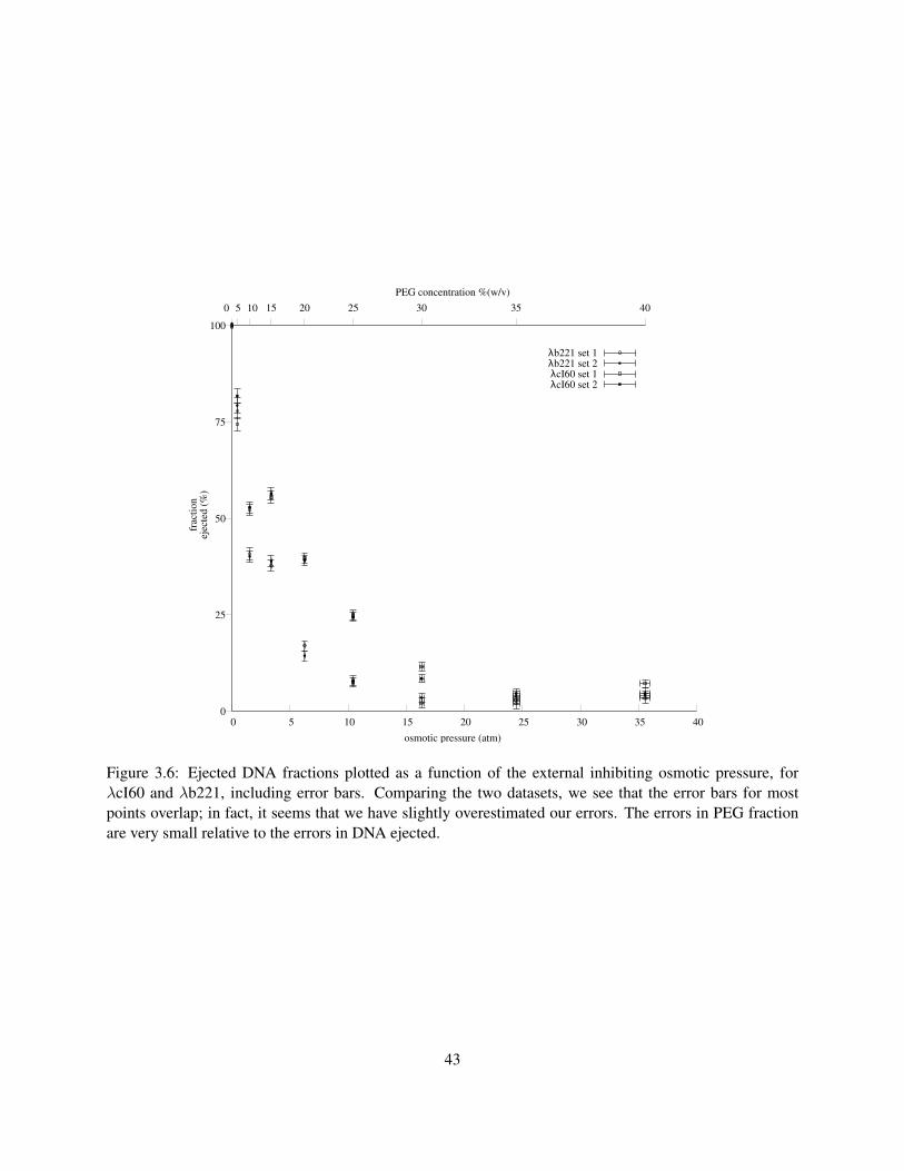
100

75

50

25

0 40 35 30 25 20 15 10 5 0

403530252015

frac

tio

nej

ecte

d (

%)

osmotic pressure (atm)

PEG concentration %(w/v)

0 5 10

λb221 set 1λb221 set 2λcI60 set 1λcI60 set 2

Figure 3.6: Ejected DNA fractions plotted as a function of the external inhibiting osmotic pressure, forλcI60 and λb221, including error bars. Comparing the two datasets, we see that the error bars for mostpoints overlap; in fact, it seems that we have slightly overestimated our errors. The errors in PEG fractionare very small relative to the errors in DNA ejected.

43

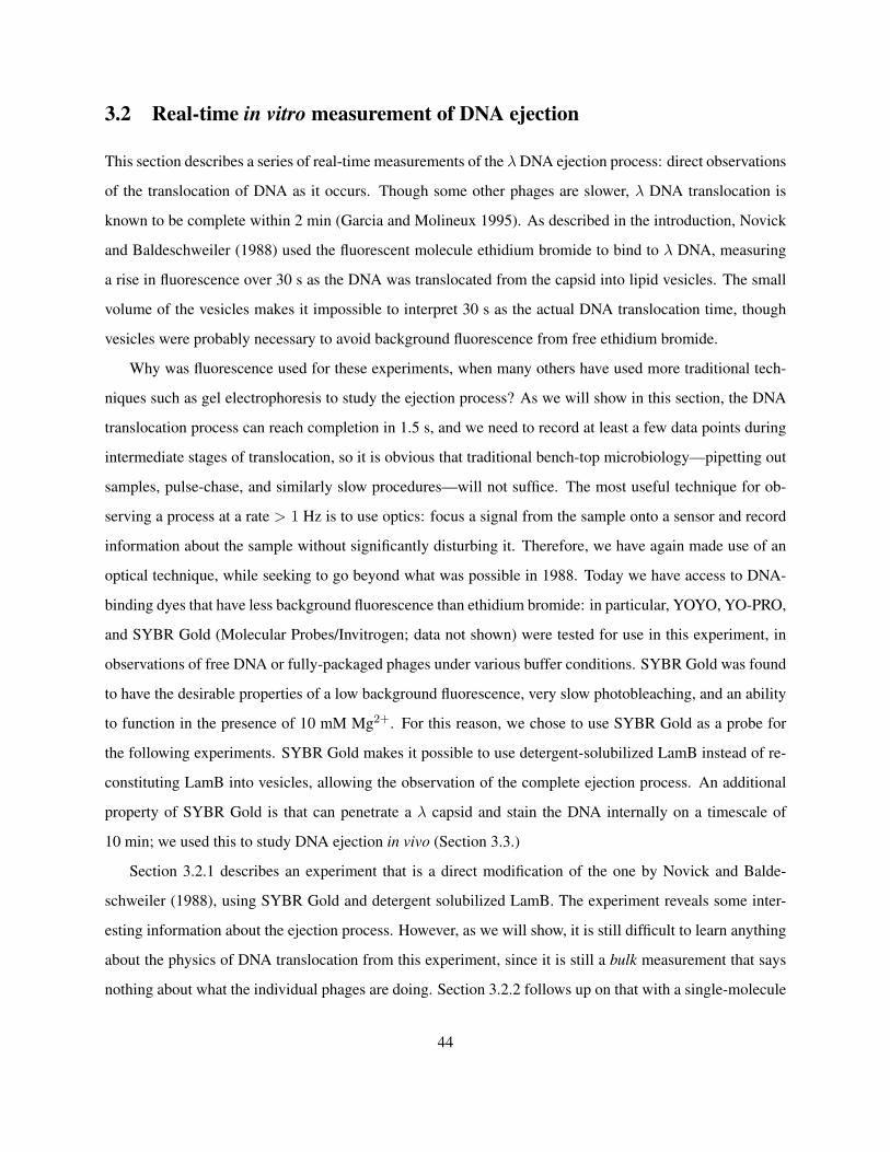
3.2 Real-time in vitro measurement of DNA ejection

This section describes a series of real-time measurements of the λ DNA ejection process: direct observations

of the translocation of DNA as it occurs. Though some other phages are slower, λ DNA translocation is

known to be complete within 2 min (Garcia and Molineux 1995). As described in the introduction, Novick

and Baldeschweiler (1988) used the fluorescent molecule ethidium bromide to bind to λ DNA, measuring

a rise in fluorescence over 30 s as the DNA was translocated from the capsid into lipid vesicles. The small

volume of the vesicles makes it impossible to interpret 30 s as the actual DNA translocation time, though

vesicles were probably necessary to avoid background fluorescence from free ethidium bromide.

Why was fluorescence used for these experiments, when many others have used more traditional tech-

niques such as gel electrophoresis to study the ejection process? As we will show in this section, the DNA

translocation process can reach completion in 1.5 s, and we need to record at least a few data points during

intermediate stages of translocation, so it is obvious that traditional bench-top microbiology—pipetting out

samples, pulse-chase, and similarly slow procedures—will not suffice. The most useful technique for ob-

serving a process at a rate > 1 Hz is to use optics: focus a signal from the sample onto a sensor and record

information about the sample without significantly disturbing it. Therefore, we have again made use of an

optical technique, while seeking to go beyond what was possible in 1988. Today we have access to DNA-

binding dyes that have less background fluorescence than ethidium bromide: in particular, YOYO, YO-PRO,

and SYBR Gold (Molecular Probes/Invitrogen; data not shown) were tested for use in this experiment, in

observations of free DNA or fully-packaged phages under various buffer conditions. SYBR Gold was found

to have the desirable properties of a low background fluorescence, very slow photobleaching, and an ability

to function in the presence of 10 mM Mg2+. For this reason, we chose to use SYBR Gold as a probe for

the following experiments. SYBR Gold makes it possible to use detergent-solubilized LamB instead of re-

constituting LamB into vesicles, allowing the observation of the complete ejection process. An additional

property of SYBR Gold is that can penetrate a λ capsid and stain the DNA internally on a timescale of

10 min; we used this to study DNA ejection in vivo (Section 3.3.)

Section 3.2.1 describes an experiment that is a direct modification of the one by Novick and Balde-

schweiler (1988), using SYBR Gold and detergent solubilized LamB. The experiment reveals some inter-

esting information about the ejection process. However, as we will show, it is still difficult to learn anything

about the physics of DNA translocation from this experiment, since it is still a bulk measurement that says

nothing about what the individual phages are doing. Section 3.2.2 follows up on that with a single-molecule

44

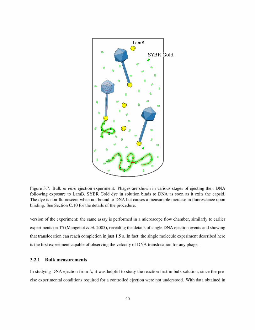
Figure 3.7: Bulk in vitro ejection experiment. Phages are shown in various stages of ejecting their DNAfollowing exposure to LamB. SYBR Gold dye in solution binds to DNA as soon as it exits the capsid.The dye is non-fluorescent when not bound to DNA but causes a measurable increase in fluorescence uponbinding. See Section C.10 for the details of the procedure.

version of the experiment: the same assay is performed in a microscope flow chamber, similarly to earlier

experiments on T5 (Mangenot et al. 2005), revealing the details of single DNA ejection events and showing

that translocation can reach completion in just 1.5 s. In fact, the single molecule experiment described here

is the first experiment capable of observing the velocity of DNA translocation for any phage.

3.2.1 Bulk measurements

In studying DNA ejection from λ, it was helpful to study the reaction first in bulk solution, since the pre-

cise experimental conditions required for a controlled ejection were not understood. With data obtained in

45

bulk, data acquisition and processing is much simpler than with single molecule data, and numerous issues

such as surface preparation are not present, making it much easier to try different reaction conditions before

moving to a single molecule measurement. We decided to use a variation of the earlier bulk fluorescence

experiment (Novick and Baldeschweiler 1988), but with sufficient dye present to monitor the entire ejec-

tion process. Unlike the former experiment, the construction of lipid vesicles was not necessary, because

the LamB was detergent solubilized and SYBR Gold has a negligible background fluorescence even when

dispersed throughout the solution. The detailed procedure for DNA ejection is given in Section C.10; see

also Figure 3.7. Essentially, a mixture of SYBR Gold dye and LamB was prepared in several wells of a

96-well plate. Phages were added simultaneously to the wells with a multi-channel pipette, and data acqui-

sition commenced immediately afterward. After the fluorescence signal stabilized, indicating that ejection

was complete, an additional set of phage aliquots was added in the same way, and data acquisition resumed.

This addition allows us to confirm that the dye was not exhausted during ejection of the first aliquot.

Assuming that solubilized LamB is a 141 kDa trimer, we calculated a final concentration of 2 · 1013

trimers/mL, far greater than the phage concentration, so that the rate of the ejection reaction was indepen-

dent of phage concentration. Such a high concentration was also required to make the rate independent of

the LamB concentration (data not shown.)

To gain an understanding of the effects of various ions on the ejection process, we compared ejection in

two buffers, with either Mg2+ or Na2+ ions at a concentration of 10 mM (see Protocols). What we expect

to see is that the force driving ejection will be significantly reduced in the Mg buffer as compared to the Na

buffer. These ions are significantly less concentrated than those within an E. coli cell, but the cytoplasmic

concentrations are not relevant for the ejection process, which takes place when the capsid is bound to the

outer surface of the cell.

Figure 3.8 shows the results of our real-time bulk ejection assay. The bulk experiment reveals several

interesting features of the ejection process. Most importantly, the fluorescence level, which is proportional

to the amount of DNA that has been released by phages, closely follows an inverted exponential curve, with

a fast initial increase that levels off as it approaches a maximum value. The process proceeds much more

quickly for λcI60 than for λb221, which seems intuitively reasonable, since λcI60 has a higher DNA density

resulting in a greater pressure (see Section 3.1.) However, the ejection process in λcI60 should actually

take more time: after a single λcI60 has released ∼10 kbp of its DNA, it becomes equivalent to a full

λb221 capsid, so its remaining DNA translocation time should be identical to the total translocation time for

46

1

0.8

0.6

0.4

0.2

0 5000 4000 3000 2000 1000 0

flu

or.

sig

nal

(re

lati

ve

un

its)

elapsed time (s)

λcI60, NaλcI60, Mgλb221, Naλb221, Mg

λcI60, Mg, no LamB

1

0.5

0 1200 800 400 0

more λ added

Figure 3.8: Characterization of ejection with bulk fluorescence. Fluorescence was measured in 5 s intervalsbeginning immediately after bacteriophages λb221 or λcI60 were pipetted into an ejection solution contain-ing SYBR Gold and LamB (see Section C.10). Here we plot the fluorescence relative to its final value forboth phages when the ejection is performed in Mg and Na buffer. The plots show that fluorescence increasesquickly at first, when many phages are ejecting their DNA, then nearly flattens out, approaching a maxi-mum value, as the ejections reach completion. Regardless of buffer, the maximum ejection is reached muchmore slowly for λcI60 than for λb221. For both phages, the Mg buffer also results in a significantly slowerejection. The signal does not completely flatten out at the end of the experiment, since SYBR Gold slowlypenetrates the capsids of phages that fail to eject their DNA. Inset: a second aliquot of phages was addedafter the first ejection was complete, resulting in an additional rise in fluorescence apparently identical tothe first. This shows that the SYBR Gold and LamB were not significantly depleted by the first addition ofphages. In the inset we show the signal that is measured when no LamB is included in the buffer. The curveswere fit to exponentials yielding time constants of 46, 94, 298, and 2870 s, respectively.

47

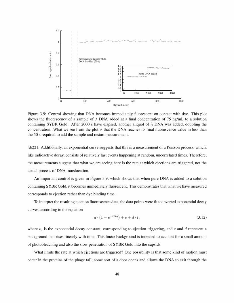
0

0.2

0.4

0.6

0.8

1

1.2

0 200 400 600 800 1000

flu

or.

sig

nal

(re

lati

ve

un

its)

elapsed time (s)

measurement pauses whileDNA is added (50 s)

0 0.2 0.4 0.6 0.8

1 1.2 1.4 1.6 1.8

4000 3000 2000 1000 0

more DNA added

Figure 3.9: Control showing that DNA becomes immediately fluorescent on contact with dye. This plotshows the fluorescence of a sample of λ DNA added at a final concentration of 75 ng/mL to a solutioncontaining SYBR Gold. After 2000 s have elapsed, another aliquot of λ DNA was added, doubling theconcentration. What we see from the plot is that the DNA reaches its final fluorescence value in less thanthe 50 s required to add the sample and restart measurement.

λb221. Additionally, an exponential curve suggests that this is a measurement of a Poisson process, which,

like radioactive decay, consists of relatively fast events happening at random, uncorrelated times. Therefore,

the measurements suggest that what we are seeing here is the rate at which ejections are triggered, not the

actual process of DNA translocation.

An important control is given in Figure 3.9, which shows that when pure DNA is added to a solution

containing SYBR Gold, it becomes immediately fluorescent. This demonstrates that what we have measured

corresponds to ejection rather than dye binding time.

To interpret the resulting ejection fluorescence data, the data points were fit to inverted exponential decay

curves, according to the equation

a · (1− e−t/t0) + c + d · t , (3.12)

where t0 is the exponential decay constant, corresponding to ejection triggering, and c and d represent a

background that rises linearly with time. This linear background is intended to account for a small amount

of photobleaching and also the slow penetration of SYBR Gold into the capsids.

What limits the rate at which ejections are triggered? One possibility is that some kind of motion must

occur in the proteins of the phage tail; some sort of a door opens and allows the DNA to exit through the

48

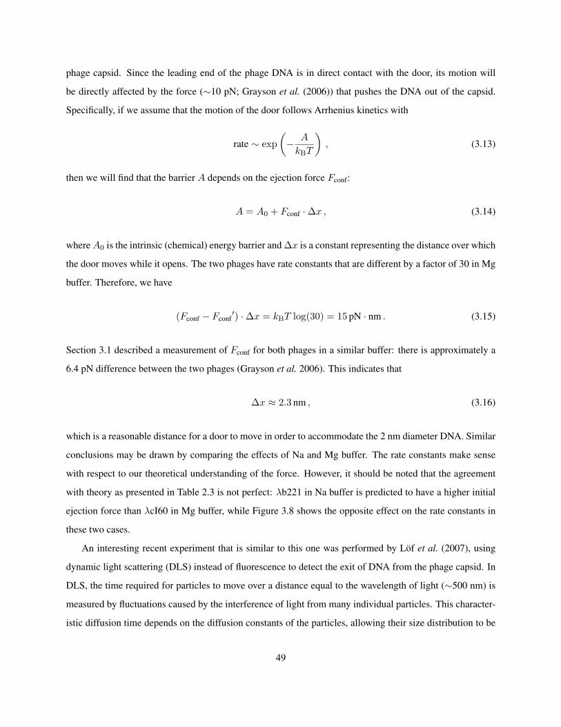
phage capsid. Since the leading end of the phage DNA is in direct contact with the door, its motion will

be directly affected by the force (∼10 pN; Grayson et al. (2006)) that pushes the DNA out of the capsid.

Specifically, if we assume that the motion of the door follows Arrhenius kinetics with

rate ∼ exp(− A

kBT

), (3.13)

then we will find that the barrier A depends on the ejection force Fconf:

A = A0 + Fconf ·∆x , (3.14)

where A0 is the intrinsic (chemical) energy barrier and ∆x is a constant representing the distance over which

the door moves while it opens. The two phages have rate constants that are different by a factor of 30 in Mg

buffer. Therefore, we have

(Fconf − Fconf′) ·∆x = kBT log(30) = 15 pN · nm . (3.15)

Section 3.1 described a measurement of Fconf for both phages in a similar buffer: there is approximately a

6.4 pN difference between the two phages (Grayson et al. 2006). This indicates that

∆x ≈ 2.3 nm , (3.16)

which is a reasonable distance for a door to move in order to accommodate the 2 nm diameter DNA. Similar

conclusions may be drawn by comparing the effects of Na and Mg buffer. The rate constants make sense

with respect to our theoretical understanding of the force. However, it should be noted that the agreement

with theory as presented in Table 2.3 is not perfect: λb221 in Na buffer is predicted to have a higher initial

ejection force than λcI60 in Mg buffer, while Figure 3.8 shows the opposite effect on the rate constants in

these two cases.

An interesting recent experiment that is similar to this one was performed by Lof et al. (2007), using

dynamic light scattering (DLS) instead of fluorescence to detect the exit of DNA from the phage capsid. In

DLS, the time required for particles to move over a distance equal to the wavelength of light (∼500 nm) is

measured by fluctuations caused by the interference of light from many individual particles. This character-

istic diffusion time depends on the diffusion constants of the particles, allowing their size distribution to be

49

determined.

Both the fluorescence experiment and the DLS experiment suffer from difficulties in interpretation due

to the fact that they are performed in bulk. There are two problems with this approach. First, data produced

in a bulk experiment is typically just a single variable that varies with time, such as the total fluorescence or

the height of a DLS peak, which must be interpreted in terms of a model of what is actually happening at the

microscopic scale. Here, we have interpreted the data as a sum of an exponential and a linear background,

where just the exponential contains the quantity of interest. However, the penetration of DNA into the

capsid may produce a background that is not linear, as binding sites for dye within the capsid become

used up. Lof et al. assumed that a “kink” in the data was due to the end of ejection and the beginning of

DNA diffusion away from the phage. However, it is not clear how such diffusion could be observed in a

DLS experiment, since the signal at each timepoint in DLS is itself produced by motions of the scattering

particles of around 500 nm; the method requires that after each timepoint, the relative positions of all of

the scattering particles are essentially randomized. Second, any bulk assay is unable to reveal what is

happening to single particles, instead producing an average property over the entire sample. We addressed

that issue here by assuming that the signal represented the total number of phages that had ejected their

DNA. However, if DNA translocation also takes a significant amount of time, the observed signal will be

a combination (mathematically, a convolution) of the triggering and ejection times. The DLS experiment

was also almost certainly observing triggering, not translocation. To see this, suppose all phages had ejected

50% of their DNA. The DLS signal would show that all of the phages had significantly reduced diffusion

constants, resulting in a characteristic time located somewhere between that of fully packaged phages and

that of free DNA; we have independently found that these two times are well separated and easy to resolve

by DLS (data not shown.) However, what was observed by Lof et al. is that the phage peak reduced in

intensity; no shift in the peak is mentioned. If the triggering was measured in the DLS experiments, it is

very difficult to understand, as was shown, that DNA binding proteins could have an effect. Curiously, there

is also no mention of the appearance of a free DNA peak after the DNA is ejected from the capsid.

All of the problems typical of bulk experiments can be resolved by performing an appropriately designed

single molecule experiment. Normally, it would be impossible to visualize phage DNA ejections directly by

microscopy, but the fluorescent dye allows microscopic visualization, as we will see in the next section.

50

Figure 3.10: Single-molecule in vitro ejection experiment. Phages are adhered to the surface of a microscopecoverslip. A solution containing LamB and SYBR Gold dye is introduced through a constant fluid flow,triggering DNA ejection. As the DNA emerges from the capsid, it immediately becomes fluorescent andmay be visualized by microscopy. See Section C.11 for the details of the procedure.

51

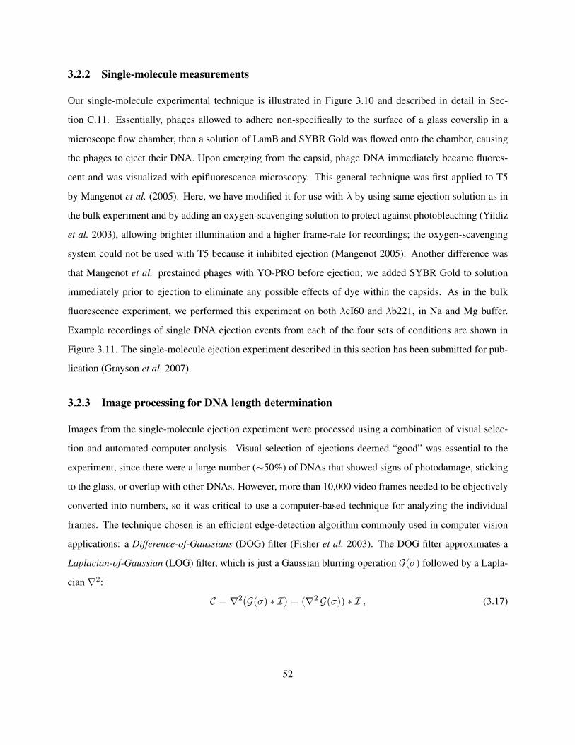
3.2.2 Single-molecule measurements

Our single-molecule experimental technique is illustrated in Figure 3.10 and described in detail in Sec-

tion C.11. Essentially, phages allowed to adhere non-specifically to the surface of a glass coverslip in a

microscope flow chamber, then a solution of LamB and SYBR Gold was flowed onto the chamber, causing

the phages to eject their DNA. Upon emerging from the capsid, phage DNA immediately became fluores-

cent and was visualized with epifluorescence microscopy. This general technique was first applied to T5

by Mangenot et al. (2005). Here, we have modified it for use with λ by using same ejection solution as in

the bulk experiment and by adding an oxygen-scavenging solution to protect against photobleaching (Yildiz

et al. 2003), allowing brighter illumination and a higher frame-rate for recordings; the oxygen-scavenging

system could not be used with T5 because it inhibited ejection (Mangenot 2005). Another difference was

that Mangenot et al. prestained phages with YO-PRO before ejection; we added SYBR Gold to solution

immediately prior to ejection to eliminate any possible effects of dye within the capsids. As in the bulk

fluorescence experiment, we performed this experiment on both λcI60 and λb221, in Na and Mg buffer.

Example recordings of single DNA ejection events from each of the four sets of conditions are shown in

Figure 3.11. The single-molecule ejection experiment described in this section has been submitted for pub-

lication (Grayson et al. 2007).

3.2.3 Image processing for DNA length determination

Images from the single-molecule ejection experiment were processed using a combination of visual selec-

tion and automated computer analysis. Visual selection of ejections deemed “good” was essential to the

experiment, since there were a large number (∼50%) of DNAs that showed signs of photodamage, sticking

to the glass, or overlap with other DNAs. However, more than 10,000 video frames needed to be objectively

converted into numbers, so it was critical to use a computer-based technique for analyzing the individual

frames. The technique chosen is an efficient edge-detection algorithm commonly used in computer vision

applications: a Difference-of-Gaussians (DOG) filter (Fisher et al. 2003). The DOG filter approximates a

Laplacian-of-Gaussian (LOG) filter, which is just a Gaussian blurring operation G(σ) followed by a Lapla-

cian ∇2:

C = ∇2(G(σ) ∗ I) = (∇2 G(σ)) ∗ I , (3.17)

52

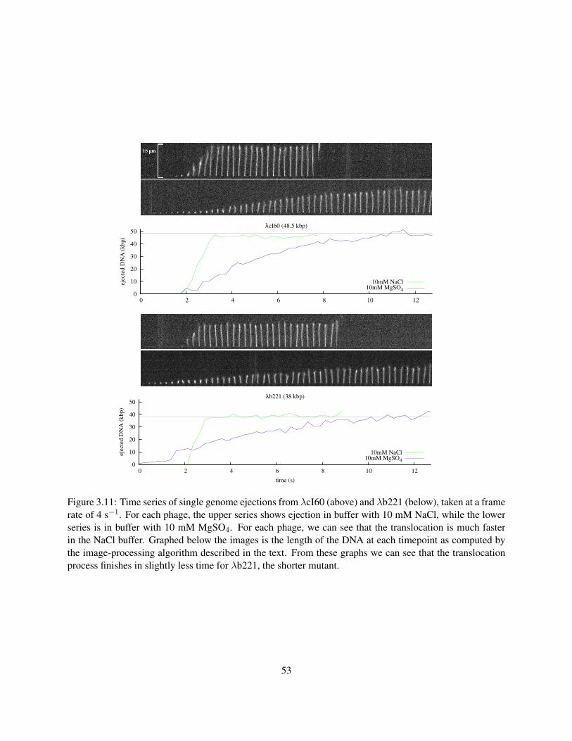
50

40

30

20

10

0 0 2 4 6 8 10 12

ejec

ted

DN

A (

kb

p)

λcI60 (48.5 kbp)

10mM NaCl10mM MgSO4

50

40

30

20

10

0 0 2 4 6 8 10 12

ejec

ted

DN

A (

kb

p)

time (s)

λb221 (38 kbp)

10mM NaCl10mM MgSO4

Figure 3.11: Time series of single genome ejections from λcI60 (above) and λb221 (below), taken at a framerate of 4 s−1. For each phage, the upper series shows ejection in buffer with 10 mM NaCl, while the lowerseries is in buffer with 10 mM MgSO4. For each phage, we can see that the translocation is much fasterin the NaCl buffer. Graphed below the images is the length of the DNA at each timepoint as computed bythe image-processing algorithm described in the text. From these graphs we can see that the translocationprocess finishes in slightly less time for λb221, the shorter mutant.

53

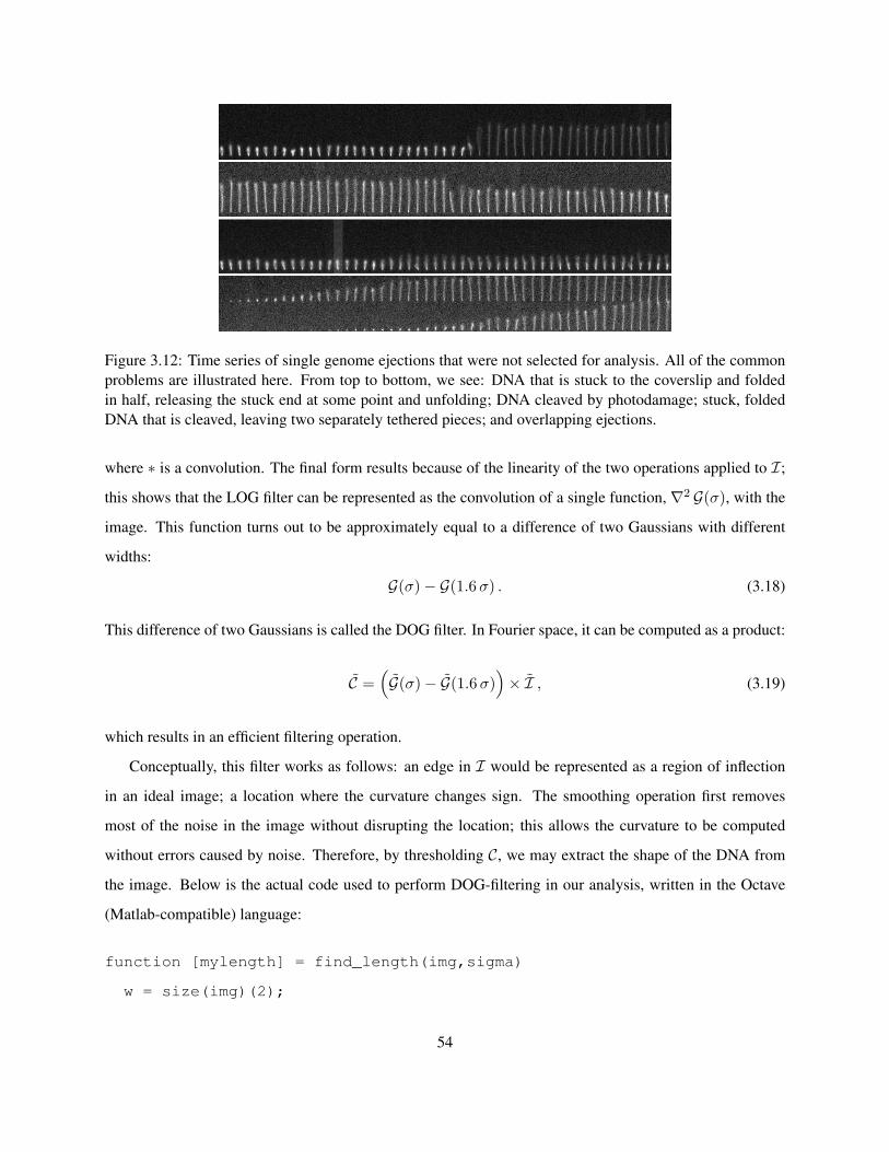
Figure 3.12: Time series of single genome ejections that were not selected for analysis. All of the commonproblems are illustrated here. From top to bottom, we see: DNA that is stuck to the coverslip and foldedin half, releasing the stuck end at some point and unfolding; DNA cleaved by photodamage; stuck, foldedDNA that is cleaved, leaving two separately tethered pieces; and overlapping ejections.

where ∗ is a convolution. The final form results because of the linearity of the two operations applied to I;

this shows that the LOG filter can be represented as the convolution of a single function, ∇2 G(σ), with the

image. This function turns out to be approximately equal to a difference of two Gaussians with different

widths:

G(σ)− G(1.6 σ) . (3.18)

This difference of two Gaussians is called the DOG filter. In Fourier space, it can be computed as a product:

C =(G(σ)− G(1.6 σ)

)× I , (3.19)

which results in an efficient filtering operation.

Conceptually, this filter works as follows: an edge in I would be represented as a region of inflection

in an ideal image; a location where the curvature changes sign. The smoothing operation first removes

most of the noise in the image without disrupting the location; this allows the curvature to be computed

without errors caused by noise. Therefore, by thresholding C, we may extract the shape of the DNA from

the image. Below is the actual code used to perform DOG-filtering in our analysis, written in the Octave

(Matlab-compatible) language:

function [mylength] = find_length(img,sigma)

w = size(img)(2);

54

h = size(img)(1);

## generate the filter function

g1 = zeros(h,w);

g2 = zeros(h,w);

for i=1:h

for j=1:w

ii = min(i-1,h+1-i);

jj = min(j-1,w+1-j);

g1(i,j) = exp(-(ii**2+jj**2)/(2*sigma**2));

g2(i,j) = exp(-(ii**2+jj**2)/(2*(sigma*1.6)**2));

end

end

g1 /= sum(sum(g1));

g2 /= sum(sum(g2));

dog = g1-g2;

## compute the curvature, C

dog_f = fft2(dog);

img_f = fft2(img);

C = real(ifft2(img_f.*dog_f));

## compute the thresholded image, T

cutoff = 0.2 * max(max(C));

T = curvature > cutoff;

...

mylength = rightedge - leftedge;

55

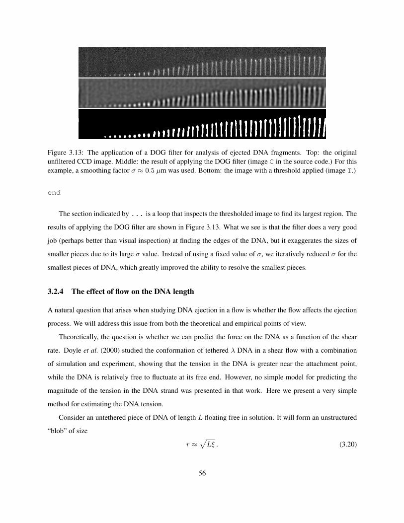
Figure 3.13: The application of a DOG filter for analysis of ejected DNA fragments. Top: the originalunfiltered CCD image. Middle: the result of applying the DOG filter (image C in the source code.) For thisexample, a smoothing factor σ ≈ 0.5 µm was used. Bottom: the image with a threshold applied (image T.)

end

The section indicated by ... is a loop that inspects the thresholded image to find its largest region. The

results of applying the DOG filter are shown in Figure 3.13. What we see is that the filter does a very good

job (perhaps better than visual inspection) at finding the edges of the DNA, but it exaggerates the sizes of

smaller pieces due to its large σ value. Instead of using a fixed value of σ, we iteratively reduced σ for the

smallest pieces of DNA, which greatly improved the ability to resolve the smallest pieces.

3.2.4 The effect of flow on the DNA length

A natural question that arises when studying DNA ejection in a flow is whether the flow affects the ejection

process. We will address this issue from both the theoretical and empirical points of view.

Theoretically, the question is whether we can predict the force on the DNA as a function of the shear

rate. Doyle et al. (2000) studied the conformation of tethered λ DNA in a shear flow with a combination

of simulation and experiment, showing that the tension in the DNA is greater near the attachment point,

while the DNA is relatively free to fluctuate at its free end. However, no simple model for predicting the

magnitude of the tension in the DNA strand was presented in that work. Here we present a very simple

method for estimating the DNA tension.

Consider an untethered piece of DNA of length L floating free in solution. It will form an unstructured

“blob” of size

r ≈√

Lξ . (3.20)

56

Near the coverslip, the DNA experiences shear flow—a flow with linearly increasing velocity—characterized

by the shear parameter j. For example, a value j = 10 s−1 means that at a distance of 2 µm from the cover-

slip, the velocity is j ·2µm = 20µm · s−1. The force on the DNA depends on the value of j. Let us make the

assumption that a portion of the DNA at the free end, having length L0, is under negligible tension, while

the remainder, of length L − L0, is fully extended. The tension in the extended DNA comes from the free

end, which forms a ball of size√

0.34 nm/bp · L0ξ. If the ball lies flush against the wall, it occupies a space

out to a distance r. The average velocity of the flow over this region is vavg = jr/2. The force on the ball

can be very roughly approximated with the Stokes formula

Fdrag = 6πηrvavg . (3.21)

How much force is required to fully extend a piece of DNA? When we say that DNA is extended, we mean

that it is no longer free to bend significantly under thermal motion; this requires the addition of free energy

on the order of 1 kT for each persistence length ξ that is to be extended, so the tension is

Fextension ≈ 1kT/ξ = 0.1 pN . (3.22)

This simplistic estimate predicts a tension that is independent of the amount of DNA that is extended.

Assuming that Fdrag balances Fextension, we can compute the amount of DNA in the ball:

L0 = kT/(3πηjξ2

). (3.23)

For the values of shear used in this experiment (see below) of 57 s−1 and 14 s−1, this expression leads to

values for L0 of 9.1 kbp and 37 kbp, respectively, which are satisfyingly close to our calibrated values of

L0 (Table 3.1). This suggests that the model is close to being correct, implying a force of 0.1 pN that is

insignificant compared to the typical value of Fconf expected to be driving DNA ejection, approximately

10 pN. At the very end of ejection, the driving force will eventually drop below 0.1 pN, but since we do not

understand what causes DNA to remain attached to the capsid for such a long time at the end of the ejection

process, it is not clear what effect, if any, the additional force from the flow will have on detachment.

For further validation that the flow does not have a significant effect on the ejection process, we have

performed the ejection assay under various flow rates, comparing the trajectories of DNA translocation that

result. Specifically, Figure 3.14 shows the recordings of DNA ejection events obtained under two shear

57

50

40

30

20

10

0 0 5 10 15 20 25

ejec

ted

DN

A (

kb

p)

time (s)

λcI60 (48.5 kbp), effect of flow in 10mM MgSO4

40 uL/min10 uL/min

40

30

20

10

05040302010 0

DN

A v

elo

city

(k

bp

/s)

DNA remaining in capsid (kbp)

λcI60 (48.5 kbp), effect of flow in 10mM MgSO4

40 uL/min10 uL/min

Figure 3.14: The effect of flow on DNA ejection. Top: an overlay of trajectories recorded under flowsof 40 µL/ min and 10 µL/min. The trajectories fall roughly over each other, within the accuracy of theexperiment, though the data is noisier at the lower flow rate. Bottom: comparison of the velocities measuredfor the two flow rates. Except for what appears to be systematic error in the middle of the graph, thevelocities are closely aligned. In any case, the translocation velocity at the higher flow rate does not appearto be faster than at the lower flow rate.

58

rates that differ by a factor of 4, as well as a velocity profile. What we see from the figure is that the DNA

translocation process does not seem to be significantly affected by the flow.

3.2.5 Length calibration

The procedure discussed so far describes how we made real-time observations of the bacteriophage λ ejec-

tion process using fluorescence microscopy. The result of these experiments is a measurement of the amount

of DNA that has emerged from the capsid, quantified in terms of xpx, the number of pixels imaged by the

CCD. The magnification factor of the microscope under our imaging conditions was calibrated:

xreal = xpx · 66 nm/px . (3.24)

However, the DNA is not ever stretched out to its contour length of L · 0.34 nm/bp, so we can not directly

compute the length of the DNA in bp from our microscope measurements. The theoretical discussion (Sec-

tion 3.2.2) of the state of the DNA in a flow suggests the general form of the relation between L and xreal, but

the theory is not solid enough to make direct quantitative predictions. Instead, we have left one parameter

free and applied fitting to experimental data on pieces of DNA with known lengths. As a final step, we have

compared the value of the fitting parameter to the rough theoretical predictions. This flexible calibration

procedure gives us confidence that we have some theoretical understanding of the DNA extension, without

sacrificing the quality of our results by forcing it to conform to an inaccurate theory.

The detailed experimental procedure for recording DNA calibration data is given in Section C.14. Essen-

tially, following the technique of Han et al. (2007), biotinylated λ DNA was cut with appropriate restriction

enzymes into pieces of various sizes, from 3.5 kbp to the full-length of 48.5 kbp. The biotin at the left

end of the DNA allowed an attachment to streptavidin within a flow chamber, and the tethered DNA was

observed under the same flow rates and using precisely the same buffers as in the in vitro ejection exper-

iment. For each tethering experiment and set of conditions, several DNA tethers were identified within a

100-frame (25 s) video and analyzed using the same image-processing subroutine that was applied in the

ejection experiment. It was necessary to exclude incorrectly-sized pieces from the analysis; we assume that

these correspond to either incomplete digestion, non-specific digestion, or non-specifically tethered pieces of

DNA. Some pieces of DNA broke due to photodamage within 25 s; the portion of the video after the break-

ing event was excluded from analysis. Figure 3.16 shows the distribution of xpx values for each measured

L.

59

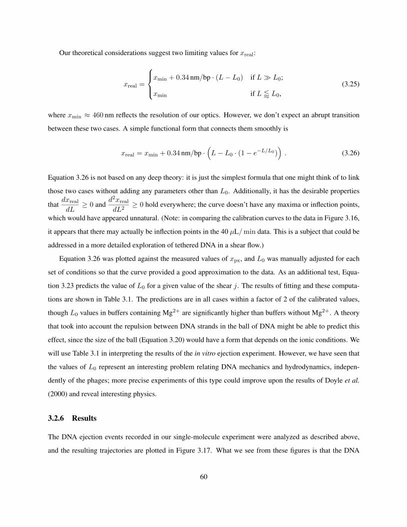
Our theoretical considerations suggest two limiting values for xreal:

xreal =

xmin + 0.34 nm/bp · (L− L0) if L � L0;

xmin if L / L0,(3.25)

where xmin ≈ 460 nm reflects the resolution of our optics. However, we don’t expect an abrupt transition

between these two cases. A simple functional form that connects them smoothly is

xreal = xmin + 0.34 nm/bp ·(L− L0 · (1− e−L/L0)

). (3.26)

Equation 3.26 is not based on any deep theory: it is just the simplest formula that one might think of to link

those two cases without adding any parameters other than L0. Additionally, it has the desirable properties

thatdxreal

dL≥ 0 and

d2xreal

dL2≥ 0 hold everywhere; the curve doesn’t have any maxima or inflection points,

which would have appeared unnatural. (Note: in comparing the calibration curves to the data in Figure 3.16,

it appears that there may actually be inflection points in the 40 µL/ min data. This is a subject that could be

addressed in a more detailed exploration of tethered DNA in a shear flow.)

Equation 3.26 was plotted against the measured values of xpx, and L0 was manually adjusted for each

set of conditions so that the curve provided a good approximation to the data. As an additional test, Equa-

tion 3.23 predicts the value of L0 for a given value of the shear j. The results of fitting and these computa-

tions are shown in Table 3.1. The predictions are in all cases within a factor of 2 of the calibrated values,

though L0 values in buffers containing Mg2+ are significantly higher than buffers without Mg2+. A theory

that took into account the repulsion between DNA strands in the ball of DNA might be able to predict this

effect, since the size of the ball (Equation 3.20) would have a form that depends on the ionic conditions. We

will use Table 3.1 in interpreting the results of the in vitro ejection experiment. However, we have seen that

the values of L0 represent an interesting problem relating DNA mechanics and hydrodynamics, indepen-

dently of the phages; more precise experiments of this type could improve upon the results of Doyle et al.

(2000) and reveal interesting physics.

3.2.6 Results

The DNA ejection events recorded in our single-molecule experiment were analyzed as described above,

and the resulting trajectories are plotted in Figure 3.17. What we see from these figures is that the DNA

60

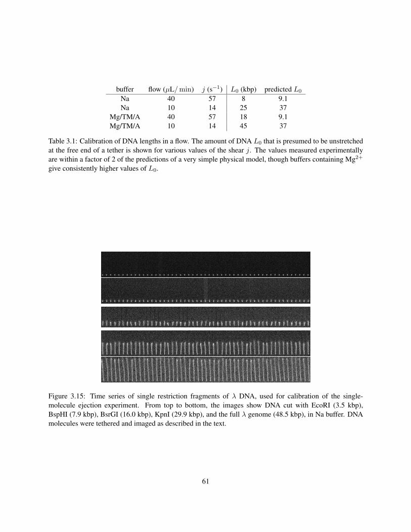
buffer flow (µL/ min) j (s−1) L0 (kbp) predicted L0

Na 40 57 8 9.1Na 10 14 25 37

Mg/TM/A 40 57 18 9.1Mg/TM/A 10 14 45 37

Table 3.1: Calibration of DNA lengths in a flow. The amount of DNA L0 that is presumed to be unstretchedat the free end of a tether is shown for various values of the shear j. The values measured experimentallyare within a factor of 2 of the predictions of a very simple physical model, though buffers containing Mg2+

give consistently higher values of L0.

Figure 3.15: Time series of single restriction fragments of λ DNA, used for calibration of the single-molecule ejection experiment. From top to bottom, the images show DNA cut with EcoRI (3.5 kbp),BspHI (7.9 kbp), BsrGI (16.0 kbp), KpnI (29.9 kbp), and the full λ genome (48.5 kbp), in Na buffer. DNAmolecules were tethered and imaged as described in the text.

61

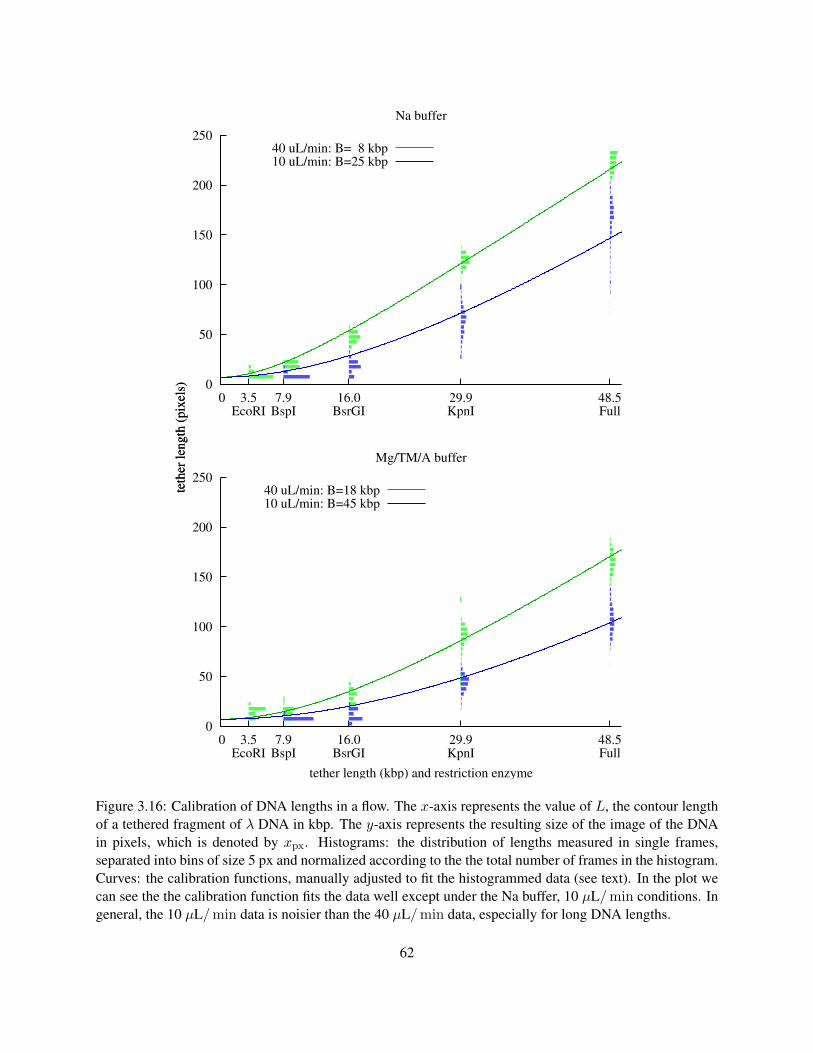
0

50

100

150

200

250

48.5Full

29.9KpnI

16.0BsrGI

7.9BspI

3.5EcoRI

0

Na buffer

teth

er l

eng

th (

pix

els)

40 uL/min: B= 8 kbp10 uL/min: B=25 kbp

0

50

100

150

200

250

48.5Full

29.9KpnI

16.0BsrGI

7.9BspI

3.5EcoRI

0

tether length (kbp) and restriction enzyme

Mg/TM/A buffer

teth

er l

eng

th (

pix

els)

40 uL/min: B=18 kbp10 uL/min: B=45 kbp

Figure 3.16: Calibration of DNA lengths in a flow. The x-axis represents the value of L, the contour lengthof a tethered fragment of λ DNA in kbp. The y-axis represents the resulting size of the image of the DNAin pixels, which is denoted by xpx. Histograms: the distribution of lengths measured in single frames,separated into bins of size 5 px and normalized according to the the total number of frames in the histogram.Curves: the calibration functions, manually adjusted to fit the histogrammed data (see text). In the plot wecan see the the calibration function fits the data well except under the Na buffer, 10 µL/ min conditions. Ingeneral, the 10 µL/ min data is noisier than the 40 µL/ min data, especially for long DNA lengths.

62

translocation process is significantly faster than what was observed in bulk by us as well as by Novick and

Baldeschweiler (1988) and Lof et al. (2007). For λcI60, the ejection time is 1.5 s in Na buffer and 8–11 s

in Mg buffer. This validates our conclusion that the bulk experiments measure the triggering process rather

than the translocation itself; due to the stochastic nature of triggering, single-molecule experiments are the

only way to get at the dynamics of translocation.

Figure 3.17 shows that the ejections are reproducible: all of the differences between the trajectories

at one set of conditions can be attributed to experimental noise or photodamage. This situation provides

a contrast with phage T5 (Mangenot et al. 2005), where DNA pausing dominated the observed ejection

process, and the velocity between steps was too high to be resolved. The one exception to the reproducibility

of trajectories is that there is a long pause at the very end of ejection: though almost all of the DNA has

emerged from the capsid in a few seconds, it is often not completely released for as long as several minutes.

This could be caused, for example, by the 12 bp single-stranded overhang of λ DNA forming hydrogen

bonds with proteins in the capsid. However, the present technique does not have the resolution to address

exactly how much of the DNA is left inside during the pause.

The translocation speed is a basic quantity of the ejection process that we can compute for the first time

based on the results of this experiment. The speed is plotted in Figure 3.18. What we see from the graph

is that most of the variation in speed is explained by the difference in buffer conditions: in a given buffer,

the speed is only determined by how much DNA remains in the capsid, independent of the original genome

length. The graphs reveal that a maximum of about 60 kbp/s is reached in NaCl buffer, while the maximum

in MgSO4 buffer is about 17 kbp/s. The simplest explanation for this is that the force was predicted to

be higher for NaCl buffer in Section 2.1.3. However, the maximum speed does not occur at the beginning

of ejection, where we expect the force to be highest, but rather at an intermediate stage of ejection. This

can be seen particularly clearly for λcI60 in Figure 3.11; there appears to be a long period of very slow

translocation when only a small amount of DNA has emerged from the capsid.

Figure 3.19 shows a plot of the inverse of velocity, which may be integrated to compute a total translo-

cation time. This results in values from 1.2 to 11.6 s, depending on the phage and buffer type, which may

be compared to the original time series plots in Figure 3.11.

Section 2.2 introduced the concept of a mobility parameter µ that determines how fast the DNA moves

in proportion to the force, and various models were proposed to predict how µ might vary with the amount

of DNA within the capsid. Our measurements of velocity now provide a way to test for the models, which

63

50

40

30

20

10

0 0 5 10 15 20 25

ejec

ted

DN

A (

kb

p)

λcI60 (48.5 kbp)

10mM NaCl 10mM MgSO4

50

40

30

20

10

0 0 5 10 15 20 25

ejec

ted

DN

A (

kb

p)

λb221 (38 kbp)

10mM NaCl 10mM MgSO4

50

40

30

20

10

0 0 5 10 15 20 25

ejec

ted

DN

A (

kb

p)

time (s)

λcI60 (48.5 kbp), other buffers

Buffer A TM buffer

Figure 3.17: Graphs of trajectories of genome ejection, comparing NaCl and MgSO4 buffers and twogenome lengths. Additionally, TM buffer (used for the experiment described in Section 3.1) and BufferA, which contains both NaCl and MgSO4 (Smith et al. 2001) are compared to the standard buffers. Thetranslocation trajectories are reproducible for all phages, without any random features (such as pauses) otherthan what is attributable to experimental noise. As in Figure 3.11, it is clear that the ejection is faster in Nabuffer than in Mg buffer, and translocation of the λb221 genome takes slightly less time than λcI60. Interest-ingly, TM buffer yields the same dynamics as Mg buffer, while buffer A has a behavior that is intermediatebetween the Na and Mg buffers.

64

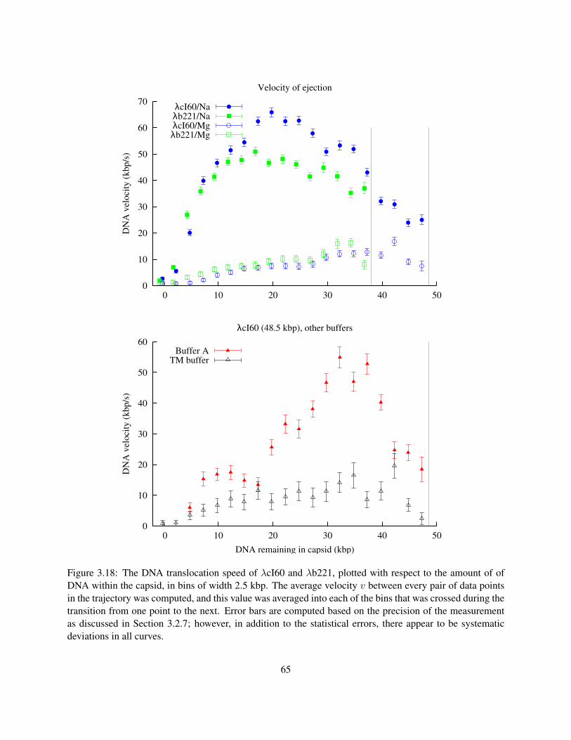
70

60

50

40

30

20

10

05040302010 0

DN

A v

elo

city

(k

bp

/s)

Velocity of ejection

λcI60/Naλb221/NaλcI60/Mgλb221/Mg

60

50

40

30

20

10

05040302010 0

DN

A v

elo

city

(k

bp

/s)

DNA remaining in capsid (kbp)

λcI60 (48.5 kbp), other buffers

Buffer ATM buffer

Figure 3.18: The DNA translocation speed of λcI60 and λb221, plotted with respect to the amount of ofDNA within the capsid, in bins of width 2.5 kbp. The average velocity v between every pair of data pointsin the trajectory was computed, and this value was averaged into each of the bins that was crossed during thetransition from one point to the next. Error bars are computed based on the precision of the measurementas discussed in Section 3.2.7; however, in addition to the statistical errors, there appear to be systematicdeviations in all curves.

65

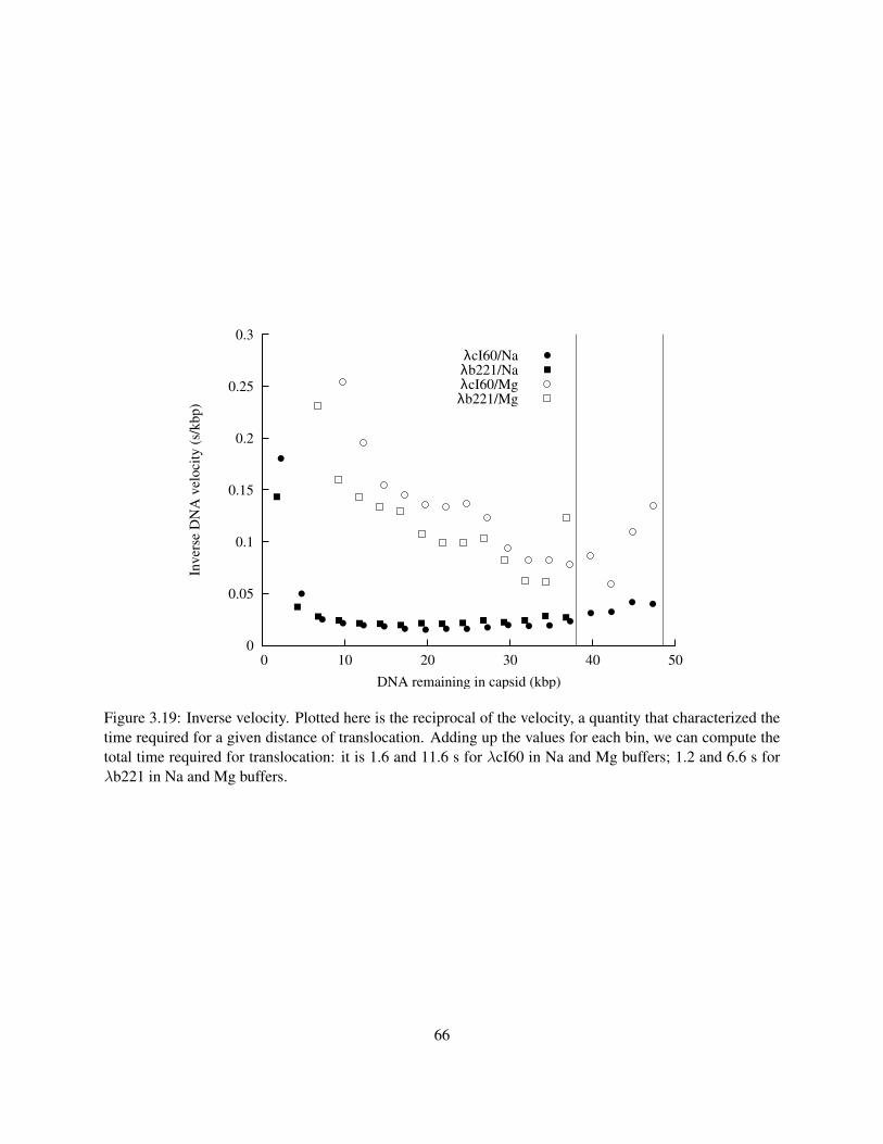
0

0.05

0.1

0.15

0.2

0.25

0.3

5040302010 0

Inv

erse

DN

A v

elo

city

(s/

kb

p)

DNA remaining in capsid (kbp)

λcI60/Naλb221/NaλcI60/Mgλb221/Mg

Figure 3.19: Inverse velocity. Plotted here is the reciprocal of the velocity, a quantity that characterized thetime required for a given distance of translocation. Adding up the values for each bin, we can compute thetotal time required for translocation: it is 1.6 and 11.6 s for λcI60 in Na and Mg buffers; 1.2 and 6.6 s forλb221 in Na and Mg buffers.

66

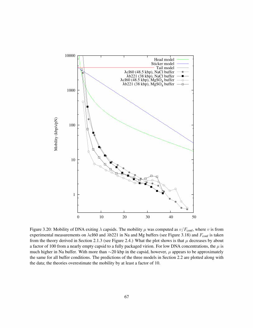
1

10

100

1000

10000

0 10 20 30 40 50

Mo

bil

ity

(k

bp

/s/p

N)

Head modelSticker model

Tail modelλcI60 (48.5 kbp), NaCl bufferλb221 (38 kbp), NaCl buffer

λcI60 (48.5 kbp), MgSO4 bufferλb221 (38 kbp), MgSO4 buffer

Figure 3.20: Mobility of DNA exiting λ capsids. The mobility µ was computed as v/Fconf, where v is fromexperimental measurements on λcI60 and λb221 in Na and Mg buffers (see Figure 3.18) and Fconf is takenfrom the theory derived in Section 2.1.3 (see Figure 2.4.) What the plot shows is that µ decreases by abouta factor of 100 from a nearly empty capsid to a fully packaged virion. For low DNA concentrations, the µ ismuch higher in Na buffer. With more than ∼20 kbp in the capsid, however, µ appears to be approximatelythe same for all buffer conditions. The predictions of the three models in Section 2.2 are plotted along withthe data; the theories overestimate the mobility by at least a factor of 10.

67

0

2

4

6

8

10

12

14

16

18

0 50 100 150 200 250

λcI60 10mM NaCl, t0 = 79s

time since first ejection (s)

tota

l num

ber

of

ejec

tions

0

5

10

15

20

25

30

0 50 100 150 200 250

λcI60 10mM MgSO4, t0 = 116s

time since first ejection (s)

tota

l num

ber

of

ejec

tions

0

5

10

15

20

0 50 100 150 200 250

λb221 10mM NaCl, t0 = 166s

time since first ejection (s)

tota

l num

ber

of

ejec

tions

0

2

4

6

8

10

12

14

16

18

20

22

0 50 100 150 200 250

λb221 10mM MgSO4, t0 not measurable

time since first ejection (s)

tota

l num

ber

of

ejec

tions

Figure 3.21: The number of ejections that have been triggered as a function of time; virtual bulk resultsfrom single-molecule data. For each ejection experiment, the total number of observed ejections (startedwith the first at t = 0) is plotted as a function of time; these are the same ejections that were used for theanalysis above. Within each of the plots is an exponential least-squares fit a(1− exp(−t/t0)) + c, where t0represents the triggering time constant.

68

we present in Figure 3.20. What the plot shows is that the mobility is strongly dependent on the amount

of DNA in the capsid, dropping by a factor of more than 100 as the DNA density is increased from near

zero to that of a fully-packed capsid. The plot also compares the theoretical predictions of Section 2.2 to

the experimental data; what we see is that the theoretical models generally predict a much higher mobility

than what was measured experimentally. The model of DNA-DNA hydrodynamic drag in the head (see

Section 2.2.2) predicts a curve that has a similar shape to the data, though it is higher by about an order

of magnitude. We infer from this result that most of the friction during DNA ejection in λ is probably

due to interactions within the head, but that the magnitude of the drag is not modeled accurately by simply

extrapolating macroscopic viscosity down to the molecular level.

An interesting exercise is to use the single-molecule results to generate virtual bulk data: by adding up

the number of ejections that have happened as a function of time, we can compute what we would expect to

find if we measured the total fluorescence of the ejection solution. However, unlike a true bulk experiment,

the virtual bulk data has no background due to effects other than DNA ejection. For example, fluorescence

due to penetration of dye into unejected capsids simply does not enter the total that is calculated according to

this method. Using the virtual bulk data, we can perform a similar analysis to what was done in Section 3.2.1.

Here, we fit each of the curves to an exponential

a · (1− e−t/t0) + c , (3.27)

which is the same as Equation 3.12 but without the linear term d · t. (We still need the constant term c to

account for the fact that the exponential does not start at 0, due to our choice of t = 0.) In Na buffer, for

example, the two phages have values of t0 that are different by a factor of 166/79 = 2.1; this implies

(Fconf − Fconf′) ·∆x = kBT log(2.1) = 3.2 pN · nm . (3.28)

Table 2.3 predicts a difference in force of 70.7− 37.4 = 33.3 pN; this implies

∆x = 0.1 nm . (3.29)

This is about an order of magnitude smaller than the value given in Section 3.2.1, approximately the right

distance if the transition state corresponds to the rupture of a hydrogen bond. It is more likely to be close

to the correct value, since, as discussed above, there are no problems with the interpretation of the data.

69

However, here again we see that the agreement with theory is not perfect, as λb221 in Na buffer is found to

have a lower rate than λcI60 in Mg buffer, the opposite of what was predicted.

3.2.7 Error analysis

Figure 3.22 shows measurements of the DNA length over time for pieces of DNA with a known length. The

points scatter about 1–2 kbp away from the known value, due to errors from data acquisition and image

processing. We have calculated the standard deviation of measurements of the lengths at σx = 1.2 kbp

for Na buffer and 1.6 kbp for Mg buffer, and from Figure 3.16 we can see that the errors are typical of a

wide range of DNA fragments in the two buffers; we will assume that these values of σx hold for all of our

measurements of both tethers and translocating DNA. What this means is that the error for a single velocity

measurement is

σv =√

2σx

∆t=

6.8 kbp/s for Na buffer;

9.1 kbp/s for Mg buffer.(3.30)

Note that in addition to σv, which is a measure of the scattering error, there is a systematic error due to the

fact that the average of the data points in Figure 3.22 is not exactly the expected value. This systematic error

is not indicated by the error bars, but we can see that the value is of the same order of magnitude as σv. As

shown in Figure 3.16, this is simply an indication that our calibration curve does not accurately represent

the experimental data.

For the velocity measurement, the average velocity between every sequential pair of data points was

computed and averaged into bins based on the positions that were crossed between the two points. The

average velocity in a bin has an error that is reduced from σv by a factor of√

N , where N is the number of

samples in the bin. This reduced value, σv/√

N , is what is plotted as the error in Figure 3.18.

70

35.0

32.5

30.0

27.5

25.0 0 5 10 15 20 25

time (s)

Mg buffer

teth

er l

eng

th (

kb

p)

35.0

32.5

30.0

27.5

25.0 0 5 10 15 20 25

Na buffer

teth

er l

eng

th (

kb

p)

mean +/- standard deviationexpected value (29.9 kbp)

Figure 3.22: Errors in measuring the DNA tether length. The expected length of a tethered fragment of λDNA is shown with a dashed gray line. The data points are derived from individual video frames of suchtethers, processed as described in the text, and the red lines indicate the standard deviation σx of the data,which is 1.2 kbp for Na buffer and 1.6 kbp for Mg buffer. Approximately 1/3 of the data points deviate fromthe mean more than ±σ, as expected for a Gaussian distribution.

71

3.3 Real-time in vivo measurement of DNA ejection

The experiment described in Section 3.2 reveals information about how the DNA exits a λ capsid in vitro,

driven by internal forces. However, this says little about the transfer of DNA in vivo, since there will be

additional forces acting on the DNA that could speed up or slow down translocation. In Section 2.3.1, we

assumed a value of Π = 0.3 pN/nm2 for the osmotic pressure in E. coli. This osmotic pressure will produce

a force the resists the translocation of DNA. To see the magnitude of this force, suppose that the pressure is

applied directly to the cross-sectional area of DNA. This would result in a force of Π · πr2DNA ≈ 1 pN. This

value is actually a significant amount of force: by examining Figure 3.5, we see that it is enough to hold

about half of the λ genome in the capsid, leading to the question of what is responsible for translocating the

remainder of the DNA.

Brownian diffusion is not expected to complete translocation: 1 kBT = 4.28 pN nm of energy is enough

to move 4.28/0.3 nm = 14 nm—only 42 bp—against the osmotic pressure. This suggests a two-stage

translocation mechanism, where Fconf drives the first stage, and some other force is responsible for finishing

translocation. Section 2.3 has already presented one suggestion for the second step of translocation: a model

in which the DNA is pulled into the cell by the osmotically-driven influx of water through the phage tail.

Another force was shown to be present in phage T7, where RNA polymerase is responsible for translocating

almost the entire genome (Garcia and Molineux 1995; Molineux 2001; Kemp et al. 2004). In the case of

φ29, there is evidence for a division of the translocation into two stages, where the first stage is driven by

Fconf and the mechanism of the second stage is unknown (Gonzalez-Huici et al. 2004). However, DNA

ejection has never been observed at the single molecule level, which makes it hard to draw conclusions

about the details of the translocation mechanism. In particular, λ is known to eject its complete genome in

vivo in less than 2 min (Garcia and Molineux 1995), though we showed in Section 3.2.1 that initiation of

ejection itself can take minutes; this means that it is probably impossible to resolve the details of the in vitro

translocation process with a bulk experiment.

Specific stages of the viral infection process have been observed at the single molecule level in vivo

in eukaryotic systems. In one study, the entry of individual influenza viruses was observed using a two-

color fluorescence technique where the viral membrane and cellular clathrin involved in endocytosis were

separately labeled with dyes of different spectra. What was found in this study is that two-thirds of the

time, influenza virions enter via clathrin-mediated endocytosis (Rust et al. 2004). A second microscopy

study followed single RNAs of influenza viruses during movement through the cytoplasm and nucleus,

72

using fluorescent dye attached to the RNAs (Babcock et al. 2004). It is interesting that the infection process

has been studied successfully at the single-particle level for influenza, while such views of bacteriophages

remain elusive.

A series of experiments involving fluorescently labeled phages points toward the possibility of studying

the phage infections at the single-molecule level. Most interest in fluorescent phages comes from their

applications as biological sensors for bacteria: Goodridge et al. (1999) showed that phages specific to E. coli

O157:H7 could be labeled with the fluorescent DNA stain YOYO-1, and that their binding to cells could

be monitored. Huang et al. (2001) observed the capsids of individual bacteriophages, using covalently

linked Alexa 488 dye. Mosier-Boss et al. (2003) stained phage P22 with the dye SYBR Gold, observing its

binding to Salmonella typhimurium. Phage PP01 can be made to express GFP, allowing the visualization of

its binding to O157:H7 (Oda et al. 2004). Recently, Lee et al. (2006) used SYBR Green I to stain phages

specific to the host Microlunatus phosphovorus. In general, when the phages are stained and allowed to bind

to bacterial hosts, they are seen distributed around the cell surface. However, in the Mosier-Boss et al. study,

it was observed that P22 phages actually injected stained DNA into the cell interiors. Though the authors

were not interested in recording a movie of the process, it suggested that we should try to make real time

observations of ejection using microscopy of fluorescently stained phages.

3.3.1 Results

There are two challenges involved in the visualization of λ DNA ejection in vivo. First, healthy, growing

cells must be held in place for visualization over several hours. The agarose pad method, described com-

pletely in Section C.4 (see also Figure 3.23), describes a method for growing cells under the microscope.

Essentially, a thin rectangular slab of agarose is prepared with M9 minimal medium and glucose as a carbon

source. A drop of diluted E. coli is added to the top and allowed to dry slightly before placement of the

pad onto a microscope coverslip for visualization. The microscope stage is heated to 37◦C to encourage

cell growth. The second challenge is making the phages visible in fluorescence microscopy. We applied a

two-color technique, using Cy5 (red emission) to stain the capsid protein and SYBR Gold (green emission)

to stain the DNA. Laser excitation with 488 nm and 735 nm then allowed the simultaneous visualization

of both components, which meant that we could distinguish between ejection and mere unbinding of the

phage. Figure 3.24 shows the kind of recordings that we were able to perform with this method.

The agarose pad technique successfully allowed cells to grow with a doubling time of 1 h, somewhat

73

Figure 3.23: Single-molecule in vivo ejection experiment. Phages pre-stained with SYBR Gold and Cy5are adhered to cells, which are then sandwiched between an agarose pad and a microscope coverslip. As aphage ejects its DNA into a cell, the change in fluorescence may be visualized. See Section C.12 for thedetails of the procedure.

more slowly than the typical time in well-aerated broth of 20–30 min. Phages bound readily to cells and

could be observed to completely cover the cell surface. However, it was important to use a much lower

density of phages for these observations in order to track individual particles. Three types of phage binding

events were observed: phages could bind and then detach from the cells, bind and remain bound, or bind

and release their DNA. Figure 3.24 shows that a bound phage moves toward the poles during cell growth,

suggesting that new cell wall material is produced at the septum. In one case, we were able to observe what

appeared to be a phage ejecting its DNA into the cytoplasm: the fluorescence from SYBR Gold on the DNA

disappeared over about 1 h, while the Cy5-stained capsid remained continuously visible. The cells in this

sample were not growing rapidly, and it is likely that the ejection we observed was significantly different

from what is normal for healthy cells. Interestingly, under some conditions the DNA fluorescence actually

spread from the capsid to a ring around the cell, as if DNA had been ejected into the cytoplasm (image not

shown), but the results were not easily reproducible.

74

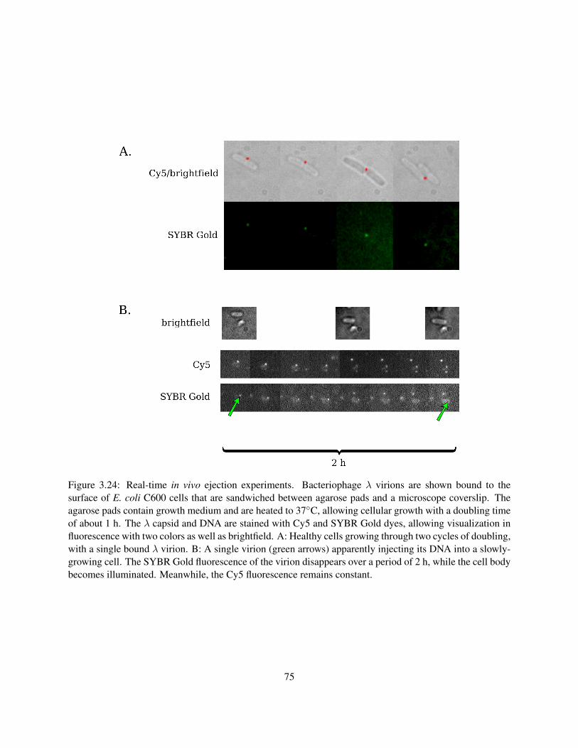
Figure 3.24: Real-time in vivo ejection experiments. Bacteriophage λ virions are shown bound to thesurface of E. coli C600 cells that are sandwiched between agarose pads and a microscope coverslip. Theagarose pads contain growth medium and are heated to 37◦C, allowing cellular growth with a doubling timeof about 1 h. The λ capsid and DNA are stained with Cy5 and SYBR Gold dyes, allowing visualization influorescence with two colors as well as brightfield. A: Healthy cells growing through two cycles of doubling,with a single bound λ virion. B: A single virion (green arrows) apparently injecting its DNA into a slowly-growing cell. The SYBR Gold fluorescence of the virion disappears over a period of 2 h, while the cell bodybecomes illuminated. Meanwhile, the Cy5 fluorescence remains constant.

75

3.3.2 Discussion

In this section, we have shown that it is possible to fluorescently label the protein capsid and DNA of λ

phages, allow them to bind to cells, and observe the phage/cell complexes over a period of hours of rapid

growth. Observing cell growth was necessary to assure that the cells were healthy and subject to DNA

injection; the agarose pad technique provided an ideal method for trapping cells under the microscope

for such a long period of time. The two-color staining of phages allows them to be uniquely identified

within a background of fragmented particles and free dye molecules, meaning that this technique might

have applications in the development of biosensors based on phage adhesion.

In several experiments, we saw what appeared to be λ DNA ejection, but the results were not conclusive.

In particular, the DNA was ejected over a 2 h timescale, much slower than the known rate of DNA ejection

from λ. It is possible that more experiments of this type would result in observations of the natural ejection

process. However, there is also a possibility that the fluorescent dyes or the observation conditions are

interfering with ejection somehow. Some experiments have been done in our lab to see whether internal

SYBR Gold affects the ejection process, but these are currently incomplete.

A future application of this experimental technique is presented by human viruses that are similar to bac-

teriophages. For example, herpes simplex virus 1 (HSV-1) has an icosahedral capsid and dsDNA genome;

it would be possible to stain the capsid and genome with exactly the same protocol that was followed here

and observe the particles inserting their DNA somehow into human cells.

76

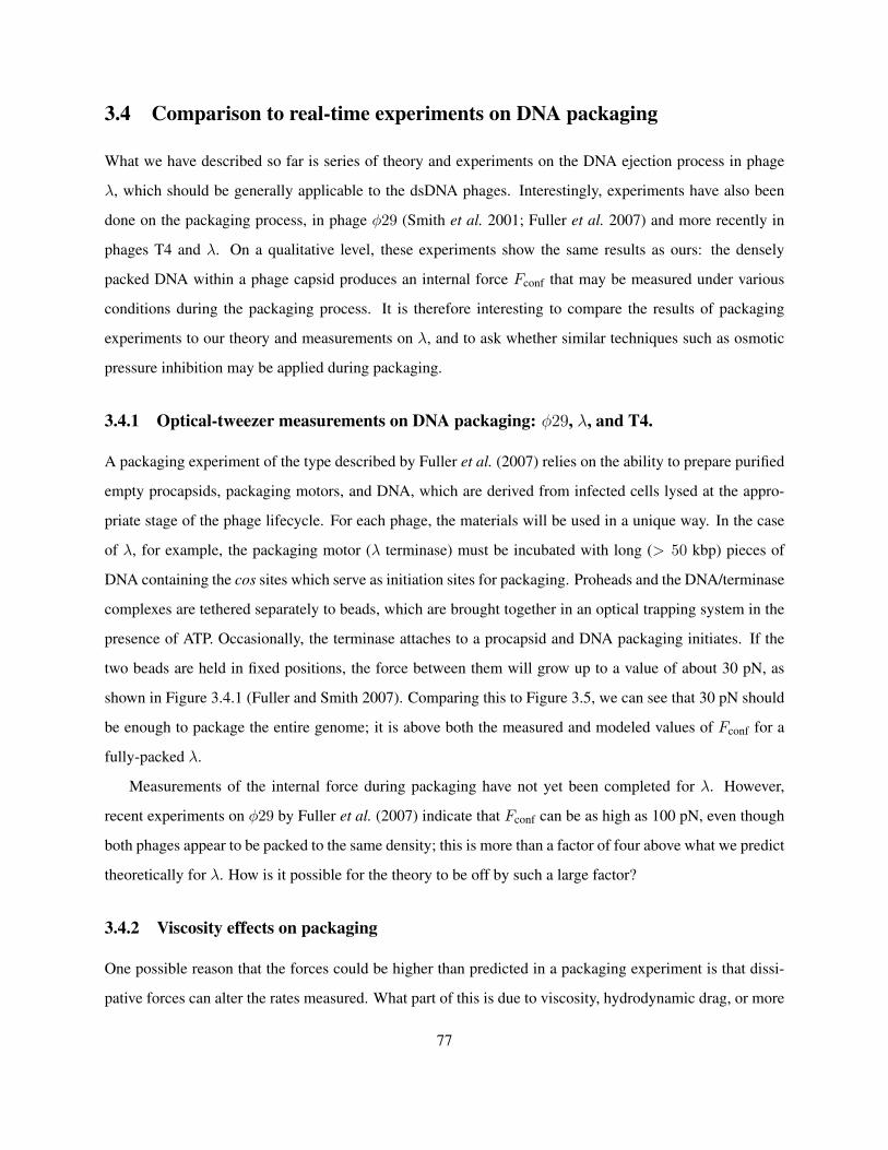
3.4 Comparison to real-time experiments on DNA packaging

What we have described so far is series of theory and experiments on the DNA ejection process in phage

λ, which should be generally applicable to the dsDNA phages. Interestingly, experiments have also been

done on the packaging process, in phage φ29 (Smith et al. 2001; Fuller et al. 2007) and more recently in

phages T4 and λ. On a qualitative level, these experiments show the same results as ours: the densely

packed DNA within a phage capsid produces an internal force Fconf that may be measured under various

conditions during the packaging process. It is therefore interesting to compare the results of packaging

experiments to our theory and measurements on λ, and to ask whether similar techniques such as osmotic

pressure inhibition may be applied during packaging.

3.4.1 Optical-tweezer measurements on DNA packaging: φ29, λ, and T4.

A packaging experiment of the type described by Fuller et al. (2007) relies on the ability to prepare purified

empty procapsids, packaging motors, and DNA, which are derived from infected cells lysed at the appro-

priate stage of the phage lifecycle. For each phage, the materials will be used in a unique way. In the case

of λ, for example, the packaging motor (λ terminase) must be incubated with long (> 50 kbp) pieces of

DNA containing the cos sites which serve as initiation sites for packaging. Proheads and the DNA/terminase

complexes are tethered separately to beads, which are brought together in an optical trapping system in the

presence of ATP. Occasionally, the terminase attaches to a procapsid and DNA packaging initiates. If the

two beads are held in fixed positions, the force between them will grow up to a value of about 30 pN, as

shown in Figure 3.4.1 (Fuller and Smith 2007). Comparing this to Figure 3.5, we can see that 30 pN should

be enough to package the entire genome; it is above both the measured and modeled values of Fconf for a

fully-packed λ.

Measurements of the internal force during packaging have not yet been completed for λ. However,

recent experiments on φ29 by Fuller et al. (2007) indicate that Fconf can be as high as 100 pN, even though

both phages appear to be packed to the same density; this is more than a factor of four above what we predict

theoretically for λ. How is it possible for the theory to be off by such a large factor?

3.4.2 Viscosity effects on packaging

One possible reason that the forces could be higher than predicted in a packaging experiment is that dissi-

pative forces can alter the rates measured. What part of this is due to viscosity, hydrodynamic drag, or more

77

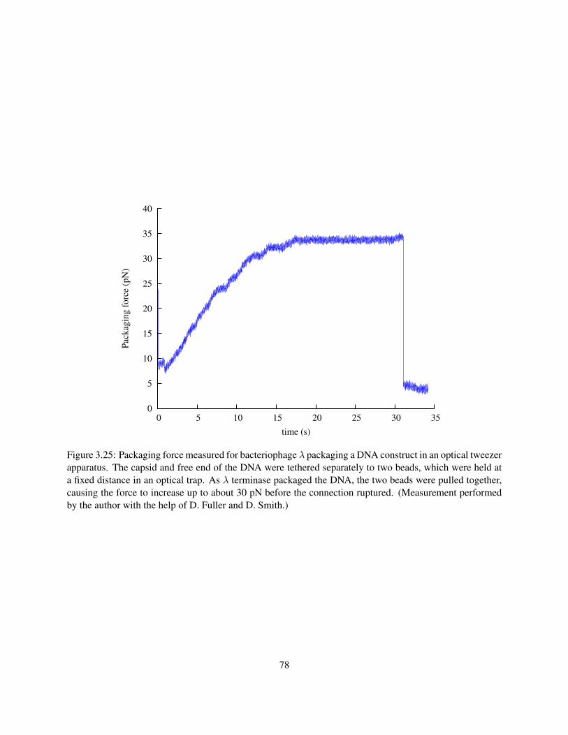
0

5

10

15

20

25

30

35

40

0 5 10 15 20 25 30 35

Pac

kag

ing

fo

rce

(pN

)

time (s)

Figure 3.25: Packaging force measured for bacteriophage λ packaging a DNA construct in an optical tweezerapparatus. The capsid and free end of the DNA were tethered separately to two beads, which were held ata fixed distance in an optical trap. As λ terminase packaged the DNA, the two beads were pulled together,causing the force to increase up to about 30 pN before the connection ruptured. (Measurement performedby the author with the help of D. Fuller and D. Smith.)

78

specific and unpredictable frictional forces?

Ejection experiments measure how fast the DNA exits a capsid when there is no motor pushing it in; the

DNA is only subject to the force from internal pressure and friction. From these measurements, it appears

that the DNA experiences more friction when the DNA density is higher, which makes sense if this friction

is due to interactions between the strands. The highest friction would then be encountered when the capsid

is fully packaged, potentially leading to errors in estimating the internal forces near the end of packaging.

In Section 3.2, we found that the mobility of DNA in a fully packaged λ capsid is about 0.5 kbp/s/pN,

independent of the buffer conditions. If φ29 encounters a similar mobility when packaging its DNA at 100–

200 kbp/s, the frictional force will be 0.05–0.1 pN, far less than the force due to pressure. Another way

of saying the same thing is that the velocities measured during single-molecule ejection experiments (as

well as slipping events during packaging) are 10–100 times higher than what is observed during packaging.

Section 2.2 predicted a mobility greater than 10 kbp/s/pN, which means that the theoretical friction is even

lower than what we measured. From both the theoretical and experimental points of view, friction appears

unlikely to play a role.

3.4.3 Osmotic pressure effects on packaging

In addition to the DNase protection assay of Section 3.1, osmotic pressure can also be used to inhibit ejection

in real-time packaging experiments, which may be useful in comparing the two experiments. In particular,

PEG concentrations of up to 10% may be applied without disrupting the packaging reaction (Fuller and

Smith 2007). There are some subtle differences between applying pressure in these different experiments;

in this section I will look carefully at what effects are important in each case.

In equilibrium, an osmotic pressure across a semi-permeable membrane sets up a hydrostatic pressure so

that the potential for water everywhere corresponds to its concentration. An osmotic pressure of, say, 10 atm

implies that there is a hydrostatic pressure of 10 atm everywhere along this semipermeable membrane,

attempting to shrink the region inaccessible to the osmolyte. In the case of PEG, which is not able to

penetrate a phage capsid, in a single-molecule packaging experiment, the excluded volume is Vbeads +

Vcapsid + VDNA. Of course, the volumes of the capsids and beads are not going to change, so the only part

that is relevant is VDNA. This does not actually correspond to the actual volume of the DNA, but to the

volume around the DNA that is excluded to PEG. As in Section 3.1, we add half the PEG monomer size of

79

0.4 nm to the DNA radius, estimating this as a cylinder of radius 1.2 nm:

VDNA ≈ π(1.2 nm)2 · L . (3.31)

For PEG with %(w/w) weight-weight fraction w, the osmotic pressure at each PEG concentration can be

determined with the empirical formula of Equation 3.2. For w = 10% at 25◦C, we find

Π = 1.8 atm = 0.2 pN/nm2 , (3.32)

which results in a force on the DNA of

F = Ππ(1.2 nm)2 = 0.8 pN . (3.33)

Effectively, this 0.8 pN will be added to the force that the motor can produce during packaging. Unfortu-

nately, we do not expect to be able to observe such a small force in the packaging experiments. If the PEG

concentration could be increased to w = 30%, we would expect an observable value of 10 pN.

3.4.4 Quantitative disagreement between theory and experiment for φ29

Our theoretical calculations predict that Fconf, the internal force on the λ DNA, is 15–40 pN, depending

on the buffer conditions. Table 2.1.2 indicates that φ29 should have a somewhat lower internal pressure.

How can we account for the recent measurements of forces in φ29 as high as 100 pN? In this section we

will carefully check the assumptions of the theory, testing whether these measurements are really out of the

range of our theoretical expectations.

Bending, as we saw in Section 2.1.4, has only a small effect on the force, even though the most sharply

bent DNA is bent to an extremely small radius. Assuming an inverse-spool model for the DNA, we expect

a force due to bending alone of 1 pN. Unless the DNA somehow gets hopelessly tangled as it is packaged,

causing Ravg to be around 2 nm, it is hard to see how bending could contribute significantly to the force.

One possibility would be if the end of the DNA is fixed during packaging, causing a huge buildup of strain

as the DNA is twisted into the capsid by the packaging motor. However, it is not known for any phage

whether the motor applies such a twist or whether the end of the DNA is fixed (Hugel et al. 2007).

Another potential source of error in our estimate of the force is that the capsid size is not known precisely.

80

Cryo-EM is probably not able to measure distances to better than 5%, and our understanding of the interface

between the DNA and the capsid is similarly unclear. For example, in φ29 there appears to be a gap of a few

nm, reducing the volume of accessible to DNA. A 5% overestimate of linear dimensions would mean that the

capsid is actually 86% of the volume estimated by cryo-EM. We can compute Fconf for λ capsids containing

1/0.86 = 116% times the full genome, finding 35 pN and 99 pN in Mg and Na buffer, respectively.

Considering these values and the values listed in Figure 2.3, the variation of the force predicted by theory

is actually very large, extending from 43–99 pN for an Na+ buffer and 15–35 pN for an Mg2+ buffer. The

values of 100 and 60 pN, measured by Fuller et al. (2007) in two similar buffers, still seem to be slightly

out of the range of what is predicted, but they are not high enough for us to be sure that unknown effects are

responsible.

81

Chapter 4

Implications and future work

This thesis presents a combination of theoretical and experimental results that together improve our under-

standing of the ejection process in bacteriophage λ and the other tailed dsDNA phages.

In Section 2.1, we compared a variety of models that predict a force pushing the DNA out during

translocation; the predicted force is close to the actual force measured by osmotic pressure inhibition in

Section 3.1. What we have learned, by comparing λ mutants with different genomes, is that the force

pushing DNA out of the capsid during in vitro DNA ejection is entirely due to the amount of DNA within

the capsid, independent of the original genome length. A model based purely on experiments on bulk DNA,

which ignores the effect of DNA bending, is sufficient to explain the force pushing the DNA out: this force

starts at about 10 pN for a fully-packed λ virion, but drops rapidly to about 1 pN after 50% of the DNA has

been ejected.

Section 2.2 addressed the dynamics of translocation, making predictions based on several sources of

friction for how fast the DNA would exit the capsid, which was compared to actual in vitro velocity mea-

surements in Section 3.2. What we have learned from these experiments is that the DNA is driven by

internal pressure, but it is limited by a source of friction that is dependent on the DNA density. The density

dependence implies that friction is due to DNA-DNA or DNA-capsid interactions in the head, rather than

in the tail. A model using the equations of hydrodynamics predicts about 10 times less friction than what

we measured experimentally. Most of our work focuses on DNA translocation, the process by which the

DNA moves out of the capsid, rather than triggering, the opening of some sort of molecular door that allows

translocation to begin. Figure 3.21 shows that we are also able to learn something about triggering from the

in vitro experiment: we see that triggering is a stochastic, Poisson-distributed process and that the phages

expected to have higher internal pressure undergo a faster triggering.

82

DNA translocation is fundamentally different in vivo, as discussed in Section 2.3 and Section 3.3. The

experimental work presented here has not been completed satisfactorily, but it suggests a path for future

work on bacteriophage ejection. We have shown that it is possible to separately label both the capsid and

genome of λ, and we have made initial observations of what may be DNA ejection events. However, the

ejection process we observed was far too slow to be representative of the natural ejection process. The speed

may be reduced due to an artifact of staining the DNA, or it may have to do with the growth state of the

bacteria. In either case, we believe that more experimentation with the staining solution and the growth

conditions will soon make it possible to see single ejections from λ or other species.

We conclude by suggesting several paths in which this research could be taken:

Perhaps most interestingly from a biological point of view, we would like to know how the DNA translo-

cation mechanism described here for phages relates to eukaryotic and especially human viruses. The virus

HSV-1 (See Table 2.1.2) is an obvious candidate for future work, as it has properties very similar to those

of the tailed bacteriophages. It is believed that HSV-1 capsids translocate their DNA into the nucleus via

the nuclear pore complex (Cardone et al. 2007), and based on our estimates of the packing density, it seems

likely that internal force from DNA compression plays a role in the translocation process. Experiments

are underway in various places to study this ejection process using real-time microscopy (Newcomb 2006;

Canaria and Bearer 2007).

The DNA tethering experiments described here suggest further physical chemistry study of the dynamics

of a tethered polymer under shear flow. We would particularly like to know about the ionic effects: why

is the DNA stretched out to a greater length in a buffer containing Na+ in one containing Mg2+? The

persistence length does not change much between these two buffers (Hagerman 1988). Doyle et al. (2000)

suggested that there was a periodic oscillation in the length of the DNA, but we have not seen evidence for

this; longer measurements and a careful mathematical analysis could help us determine whether the DNA is

best described by fluctuations about an average structure or by cyclical motion through a series of unstable

conformations.

The equilibrium pressure measurements and the real-time ejection experiments present an arena in which

a variety of questions about phage ejection may be addressed. We have used just a few buffers and variants

of λ in this study, but it would be interesting to try the experiments at various ratios of Na+ to Mg2+, to

explore the effect of DNA condensing agents such as spermine, to examine the effect of temperature, and to

try various ejection-mutants of λ and possibly LamB. All of the experiments described here are possible not

83

only in λ but also in phages T5 (Letellier et al. 2004) and SPP1 (Sao-Jose et al. 2004), which have purifiable

receptor proteins that cause ejection in vitro. However none of the experiments have been reported for

all three phages, so there is much comparative work left to be done. Beyond these phages, others could

potentially be studied using purified cell walls (Anderson 2005).

Bacteriophage capsids support a pressure that is probably close to the maximum possible without rup-

ture (Purohit et al. 2005). A recent study showed a correlation between the density of the genome within

bacteriophages and their instability under heating (Paepe and Taddei 2006); similar, unpublished data on a

variety of phage P2 deletion mutants has been communicated to me (Bertani 2005). It would be very inter-

esting to devise a theoretical model for the stability of capsids at high temperature. One point of comparison

would be phage HK97, which has a “chainmail” structure of crosslinked proteins; it has been suggested

that heating experiments on this phage could determine whether or not the unique structure gives HK97 an

increased stability (Gan 2006).

As a final point, we believe that the language used in describing the bacteriophage ejection process in this

thesis represents an important new way of looking at bacteriophages. In particular, we have demonstrated

from a number of points of view the importance of the packing ratio α introduced in Section 2.1.2; most

of the details of the ejection process depend only on α. As a humorous example of how this language is

becoming more widely used in the field, a phage was recently reported to have a value of α = 1.9 (Seaman

and Day 2007). We don’t understand how it is possible for the DNA to take up 90% more space than is

available within the capsid, but we are excited that people are beginning to think along these lines. We are

looking forward to continuing the discussion about the relationship between DNA packing and the ejection

process as the field develops.

84

Chapter 5

Acknowledgments

5.1 People

5.1.1 Collaborators

I have worked directly with the following people on this project:

• Alexander Evilevitch taught me his experimental technique during several sessions at UCLA that

extended until late in the night.

• Lin Han, a member of the Phillips lab, has been a constant help with all parts of the lab work. She

specifically contributed the protocol and technique for DNA tethering, described in Section C.14.

• Mandar Inamdar, a member of the Phillips lab, worked directly with me in deriving the physical

parameters used in Section 2.1 and was constantly of help in trying out new theoretical ideas and

suggesting directions that I could take the experiments.

• William Gelbart is a close collaborator who has worked with me on all aspects of this project. He and

Chuck Knobler lead a group of virus researchers at UCLA with which I have exchanged numerous

ideas.

• Charles Knobler is a close collaborator who has worked with me on all aspects of this project. His

ability to understand the critical details of this project has always made discussions with him essential.

• Joseph Koehler was an undergraduate summer student in the Phillips lab in 2005.

• Jane Kondev is a member of my thesis committee who participated directly in the modeling project

described in Section 2.1.

85

• Corinne Ladous was a member of the Phillips lab until 2005 who helped in all aspects of running the

lab. In addition to many other contributions, she helped me improve the precision of the protocol for

measuring ejection pressure given in Section C.7.

• Catie Lichten was a student at the MBL Physiology course who worked with me on an attempt to

measure the injection of DNA into cells in real time.

• Ian Molineux has collaborated with me on many aspects of the project, particularly the development

of the toilet-flush model.

• Kelsey Nelson-James was an undergraduate summer student in the Phillips lab who worked with me

in 2003.

• Rob Phillips has been my advisor on this project since 2002, when I enrolled at Caltech.

• Prashant Purohit was a collaborator on the work described in Section 2.1 who also provided constant

feedback on the experimental efforts.

• Erdal Toprak was another student at the MBL Physiology course who worked on the observation of

phage injection and also helped me later at UIUC.

• Zachary Travis was a high-school summer student in the Phillips lab in 2004, who investigated the

possibility of using fragmented cell membranes to cause ejection in phages for which the receptor

protein is unknown.

• Tabita Winter was a visitor in the Phillips lab, 2006–2007. She participated in the experiment of

Section 3.2 and made a major effort to get the in vivo experiments of Section 3.3 to work reliably.

5.1.2 Helpful Discussions

I would like to thank the following people for extremely helpful and enlightening discussions:

• Scott Fraser is a member of my thesis committee who is an expert on imaging techniques and also

laboratory electronics. We have had many useful discussions.

• Giuseppe Bertani is a member of my thesis committee and a local expert on λ and other phages. His

unpublished work on the relationship between pressure in P2 and its stability against thermal rupture

was part of the inspiration for this work.

86

• Zhen-Gang Wang is a member of my thesis committee and an expert in polymer physics. We have

had many productive discussions about the modeling of phage DNA.

• Elizabeth Bertani introduced me to field-inversion electrophoresis.

• Li Tai Fang is working on a continuation of the in vitro ejection experiments, and we discuss our

progress regularly.

• Lu Gan discussed issues about phage pressure with me on many occasions.

• Alexander Grosberg suggested the computation of mobility presented in Figure 3.20 as well as devis-

ing the sticking model of Section 2.2.3.

• Taekjip Ha was gave me several suggestions during my time at UIUC, especially over the weekly

social hours in his lab.

• Mindy Hoffman helped me get started using the facilities at UIUC.

• Heun Jin Lee is a postdoctoral researcher in the lab who has been very helpful and patient discussing

various things with me and who conducted a class in which I learned the basics of microscope optics.

• Sua Myong suggested the use of Cy5 for observing capsid fluorescence (Section 3.3) and kindly

donated a quantity of the dye that was sufficient for all of my experiments.

• Yan Poon helped me with the entire LamB protein purification procedure.

• Michael Rubinstein, along with Alexander Grosberg (above), gave me useful suggestions about the

mobility computation.

• Tristan Ursell is a student in the lab who has been of particular help with the microscope facility where

the experiments of Section 3.2 were performed.

• Jonathan Widom has talked to us many times about issues relating to DNA bending. Discussions with

his group were particularly memorable.

• Paul Wiggins was a student in the lab who was always willing to discuss my project and provided

many useful ideas.

• David Wu is a student in the lab who has been of great help especially with any optics-related issues.

87

5.2 Help with materials and facilities

5.2.1 Strains

• LamB and the pop154 E. coli strain: Alexandra Graff and Emir Berkane.

• λb221cI26, λcI60, and E. coli C600: Michael Feiss.

5.2.2 Laboratory space and materials

Essential parts of the project were performed in the laboratories of:

• Scott Fraser; the Beckman Imaging Center, Caltech.

• Grant Jensen; the Broad Center Cryo-EM facility, Caltech.

• Steven Mayo; his lab is located next to ours, and we are constantly sharing equipment, space, and

supplies.

• Douglas Rees; his lab provided equipment essential to our purification of LamB.

• Paul Selvin; I visited his lab for two months in 2006 to work on the in vivo ejection experiments.

• Stephen Quake; his lab was essential in helping ours grow between 2002 and 2005, and we have

maintained a constant channel of communication.

5.3 Funding

• A grant from the Keck Foundation (Rob Phillips)

• An NIH Director’s Pioneer Award (Rob Phillips)

• An NSF Graduate Research Fellowship (Paul Grayson)

• NSF grant CMS-0301657 (Rob Phillips)

• NSF grant CHE-0400363 (Charles Knobler and William Gelbart)

• Financial support from The Swedish Foundation for International Cooperation in Research and Higher

Education and the Swedish Research Council (Alexander Evilevitch)

88

Appendix A

Glossary

λb221 λb221cI26, a clear-plaque deletion mutant of phage λ with a 38 kbp genome.

λcI60 A clear-plaque mutant with a 48.5 kbp genome.

atm Atmospheres (105 Pa.)

bp Base-pair of DNA or RNA.

Buffer A 50mM TRIS 50mM NaCl 5mM MgSO4 pH 7.8 (See Section C.11.)

kbp 1000 bp.

Mg buffer 10mM TRIS 10mM MgSO4 pH 7.8 (See Section C.11.)

Na buffer 10mM TRIS 10mM NaCl pH 7.8 (See Section C.11.)

pN 10−12 N.

px Pixels.

TM buffer 50mM TRIS 10mM MgSO4 pH 7.4 (See Section C.13.)

89

Appendix B

Mathematical variables

Π0 The hypothetical pressure at zero spacing between DNA strands.

ds Center-to-center spacing between sections of hexagonally packed DNA.

Fconf Force due the internal conformation of the DNA; dGconf/dx.

Ffric Force on translocating DNA due to friction.

Fhead Drag force due to water flowing between sections of DNA in the head.

Fosm Force on translocating DNA due to osmotic pressure within the cell.

Ftail Drag force due to water flowing between the DNA and tail.

Gconf Free energy of the DNA within the capsid, due to its internal conformation.

j The shear flow parameter near the surface of the slide; dv/dz.

kB Boltzmann’s constant; kBT ≈ 4.28 pN · nm at 37◦C.

LDNA Total length of DNA.

Ltail Length of the tail tube.

Rcapsid Radius of the capsid interior (it is assumed to be spherical.)

rDNA Radius of a strand of DNA; 1 nm.

Rin Radius of the innermost DNA loops in the inverse-spool model.

rPEG The size of a PEG monomer, approximately 0.4 nm.

Rtail Radius of the interior of the tail tube.

VDNA Volume of a strand of DNA; 0.34 nm · πr2DNA.

Vcapsid Volume of the capsid.

90

Appendix C

Protocols

Note: The following protocols are copied directly from our group wiki. Therefore, some may have been

edited directly by my collaborators.

91

C.1 Bacteriophage propagation

C.1.1 Background

This procedure is the the equivalent of single-colony propagation of bacterial cell lines: single-plaque prop-

agation of phages. It is a process that is necessary for growing any genetically pure species, because it

greatly lowers the chance of the line being contaminated with a fast-growing mutant or a foreign species of

phage. To some extent, the genetic purity of a phage sample can be assessed by running DNA or protein

gels and looking for differences.

C.1.2 Materials

• 1 titer plate with distinct, clearly visible plaques

• TM buffer

• Chloroform

C.1.3 Procedure

1. Put 100ul TM buffer in a tube.

2. Using a wide-mouth pipette tip, gently remove one plaque from the plate, taking the agar below along.

3. Blow out the agar plug into the TM buffer.

4. Add a tiny drop of chloroform to the tube to kill any live cells.

5. Store for (probably) up to two years at 4◦. It is a good idea to make new stock every couple of months

or so.

92

C.2 Extraction of phage DNA

C.2.1 Background

Be careful of phenol! It can cause chemical burns. Wear gloves, work in the fume hood, and dispose of

chemicals in proper waste containers.

C.2.2 Materials

• CsCl purified phages in buffer with at most 10mM Mg

• 1.5 M TRIS 0.15 M EDTA pH 8.5

• phenol or phenol:chloroform:isoamyl alcohol solution

• chloroform

C.2.3 Procedure

1. Add 0.1 volumes of the the TRIS/EDTA solution to 1 volume of phages.

2. Leave phages at room temperature for 10 min—from this point on, use a wide mouth tip to pipette

phage DNA.

3. Add 1 volume of phenol to phages using a glass pipette.

4. Mix gently by tapping the side until it attains the appearance of a salad dressing—phenol/water col-

loidal suspension.

5. Spin briefly to separate phases:

• top phase: water + DNA

• bottom phase: phenol + protein

6. Carefully remove DNA phase with a wide-mouth pipette.

7. Add 1 volume of chloroform using a glass pipette.

8. Mix gently (you will not get a suspension this time).

9. Carefully remove DNA phase with a wide-mouth pipette.

93

C.3 Field inversion gel electrophoresis

This method for separating DNA in the range of 20-100 kbp is described in detail by Birren et al. (1990).

Essentially, 100 V is applied to the gel in the forward direction for 0.8 s, followed by 60 V in the backward

direction for 0.8 s. The slight differences between the mobilities of long DNA strands are amplified by the

differential steps, and over a period of 20 h, a high-quality separation is achieved. We use a custom-built

PWM field-inverter to perform this task in the lab and can locate bands to a precision of 100 bp.

C.3.1 Procedure

1. Prepare 0.5x TBE 1% agarose gel.

2. Load samples (remember first to heat and λ DNA samples to 65◦C and cool on ice to melt cohesive

ends).

3. Connect input of inverter box to standard gel power supply.

4. Connect gel box inputs to inverter outputs (only run one gel at a time).

5. Turn on inverter.

6. Set power supply to 100V and timer to 20 h.

7. Take care to check the periodic appearance of bubbles before leaving the gel room!

94

C.4 Growing cells on agarose pads

C.4.1 Materials

• Agarose

• M9 minimal salts media + glucose

• Standard slides and coverslips

C.4.2 Procedure

1. Prepare 1% agarose with M9 media in a 15 mL tube. The tube may be microwaved to melt the agarose.

2. Pour 3 mL agarose solution onto a slide and carefully cover with another slide, sandwiching the

agarose in between the two slides.

3. Wait until agarose has solidified

4. Gently pull the slides apart to expose a section of agarose, and excise it with a coverslip, transferring

this “pad” to another slide.

5. Put a drop of bacteria on the pad, allowing 5 minutes to dry.

6. Using the coverslip, flip the pad onto an observation dish.

7. Apply a fragment of a coverslip to the top of the agarose pad to limit drying and shrinking.

8. Seal observation dish with parafilm.

9. The sample may now be observed through a microscope objective on a heated stage. Cells should

grow with a doubling time less than 1 h.

95

C.5 Lambda plate lysis

C.5.1 Supplies

• 3 Section C.6, warmed to 37◦C

• phage stock

• rapidly growing host bacteria at an OD600 of about 0.1

• molten top agar at 45◦C

C.5.2 Procedure

1. Add 10,000, 100,000, and 1M phages to 1 mL of cells in a 15 mL Falcon tube.

2. Allow 30 min for binding at room temperature.

3. Add 10 mL top agar to each tube, invert to mix, and pour immediately onto the plates.

4. Incubate at 37◦C for 6–8 hours, until plaques almost cover the plates. (We use three different concen-

trations to make sure that we hit that regime on one of them.)

5. Add 1 drop of chloroform and TM buffer to cover plate, let set at room temperature for 2 hours or in

the cold room overnight.

6. Using a glass coverslip to direct the flow, carefully pour the buffer (containing phages) into a falcon

tube.

7. (Optional) Treat with DNase, RNase, and lysozyme to improve the phage yield and remove bacterial

junk.

8. Spin 1000 g, 10 min to pellet intact bacteria.

9. Save supernatant, which contains the phages.

96

C.6 Lambda plate lysis plates

• 10 g tryptone

• 5 g NaCl

• 2.5 g MgSO4 (which corresponds to a final concentration of roughly 10 mM)

• 20 mg FeSO4 (which corresponds to a final concentration of roughly 4 uM)

• 13 mg CaCl2 (which corresponds to a final concentration of roughly 75 uM)

• 20 g agar

• 2 mg thiamine

• water to 1 L

Mix ingredients except thiamine, and autoclave. Add sterile-filtered thiamine solution as agar is cooling

down, then pour plates half full with about 100 ml solution in each plate.

97

C.7 Osmotic pressure inhibition assay

C.7.1 Materials

• TM buffer with 1% n-octyl-oligo-oxyethylene (oPOE, Alexis Biochemicals #500-002-L005)

• TM buffer with 50% (w/w) polyethylene glycol (PEG) and 0.5% (oPOE)

• CsCl purified λ phages at a concentration of 1012 pfu/mL

• 2 mg/mL DNase I

• 20 µg/mL Section C.8 in TM buffer 1% oPOE

C.7.2 Procedure

Many samples should be prepared simultaneously at an analytical balance. Every step of the following

procedure has been optimized to reduce the error, which comes primarily from the difficulty in pipetting the

viscous PEG solution. If the steps are followed precisely, it is possible to set the concentration of PEG in

each tube to a precision of approximately 0.1%. The experiment should be tested to be independent of the

final concentration of LamB, which is the most variable parameter in the procedure.

For a 200 µL sample with x% PEG:

1. Add x mg PEG solution to 1.7 mL Eppendorf tubes at an analytical balance. The volume will be

x/1.09 µL.

2. Add 1.0024(20-x/1.09-10-1-25) mg TM buffer 1% PEG at the balance.

3. Add 10 µL phages (to the side of the tube, with an narrow-mouth tip; no mixing!)

4. Add 1 µL DNase (in the same way.)

5. Close tube and rotate slowly for several minutes to mix the solutions.

6. Add 25 µL LamB solution and mix quickly by pipetting up and down for about a minute, until the

solution is clear.

7. Incubate 1 h, 37◦C.

98

8. Centrifuge 20 h at 18,000 g.

9. Immediately after centrifugation, gently remove 120 µL supernatant to plastic UV cuvette (Ocean

Optics).

10. Measure OD260 on the spectrophotometer.

99

C.8 Purification of LamB

C.8.1 Background

This protocol uses E. coli K12 with the lamB gene from Shigella sonnei 3060 to generate concentrated lamB

protein (Graff et al. 2002). Mixing purified lamB with lambda phage causes the phage to immediately eject

their DNA into the solution. This protocol was given to me by Alex Evilevitch, but I believe it originates

with A. Graff’s lab in Basel, Switzerland.

C.8.2 Materials

• The pop154 strain of E. coli (write our lab if you want some)

• Several liters of (1x) LB medium

• Breaking buffer

– 1.34 g (50 mM) sodium phosphate

– 0.58 g (100 mM) sodium chloride

– 0.07 g (2 mM) EDTA

– 5 g sucrose

– Water to 100 ml

• 200 mM sodium phosphate buffer, pH 7.5. This can be used to make the other buffers—2 ml for a

100 ml 20 mM solution

– 26.8 g (1M) sodium phosphate

– Water to 500 ml

Adjust the pH to 7.5 then autoclave.

• Pre-extraction buffer I minus detergent. After homogenization you add 0.3% oPOE. For 20 ml solu-

tion this is 60 µL oPOE.

– 10 ml (20 mM) 200 mM sodium phosphate buffer

– Double-distilled water to 100 mL

100

• Preextraction buffer II

– 10 mL (20 mM) 200mM sodium phosphate buffer

– 500 µL (0.5%) oPOE

– Double-distilled water to 100 mL

• Extraction buffer

– 10 mL (20 mM) 200 mM sodium phosphate

– 3 mL (3%) oPOE

– Double-distilled water to 100 mL

C.8.3 Procedure

1. Start a preculture with 5 ml of LB.

2. Then 2.5 mL to 2x (1 mL pop154 + 1 mL glycerol), store at -80◦C.

3. 2.5 mL + 17.5 mL LB + 0.2% maltose at 37◦C for 6 hours

4. Put 5 mL of this culture in 2 L of LB + 0.2% maltose (use 5 L Erlenmeyer bottles) (you can make 2x

2 L with 2x 5 mL), incubate overnight.

5. Take the 4 L overnight culture and spin down on 4◦C for 30 min, 5000 rpm.

6. Take up the pellet in breaking buffer (10 mL for 1 g of pellet.)

7. Bring cells to the french press (pass 2x the supernatant) or use sonicator.

8. Spin for 10 min, 7000 rpm to remove the non-broken membranes.

9. Spin down in the ultracentrifuge at 18◦C for 40 min, 30 krpm (pellet = cell envelopes.)

10. Bring pellets into 20 mL preextraction buffer I, homogenize (first with the mixer and then add the

detergent) and incubate it for 50 min at 40◦C.

11. Spin down like step 8.

12. Bring pellets into 20 ml preextraction buffer II and incubate like step 9.

101

13. Spin down like step 8.

14. Bring pellets into 20 ml extraction buffer and incubate at 37◦C for 40 to 60 minutes.

15. Spin down in the ultracentrifuge (like step 8) and keep the supernatant = LamB.

16. Make a gel as a control (10ul + SDS sample buffer on RT and 95◦C for 10 min.)

17. Dialyse against 1% oPOE + Na phosphate buffer pH 7.5

18. Column affinity purification (amylose resin from NEB), elution with 20% maltose in 1% oPOT + Na

phosphate buffer pH 7.5.

19. Remove maltose by dialysis against 1% oPOE + Na phosphate buffer pH 7.5.

102

C.9 Purification of λ

C.9.1 Supplies

• 10 mL of phages at 1011/mL or more

• TM buffer

• CsCl

C.9.2 Differential sedimentation

1. Spin phages at 1000 g, 10 min to pellet intact any precipitated junk (DNA, bacteria, etc.)

2. Spin supernatant at 30 krpm for 2.5 h in the 60 Ti rotor. Turn off the brake for this spin so that the

phages can come to a gentle stop; be ready to take them out as soon as the spinning stops.

3. Gently pour supernatant off, wiping the last drops with a Kimwipe. There should be a visible white

pellet in the bottom of the tube.

4. Add 1–2 mL of TM buffer to the top of the pellet.

5. Allow 2 h at 4◦C or overnight for phages to dissolve into the pellet.

6. Remove liquid (and scrape off any remaining pellet) using a plastic transfer pipette; store in an Ep-

pendorf tube.

7. Spin at 1000 g, 10 min to pellet junk.

8. Save supernatant or use immediately for CsCl gradient.

C.9.3 CsCl gradient

1. Prepare CsCl/phage mixture at density of the phages. You will want to experiment with this; I use

1.388 g CsCl powder + 1.612 mL phage/TM solution, mixed directly together in a 3 mL swinging-

bucket centrifuge tube.

2. Spin in TLS-55 overnight at 30 krpm.

3. If there is a layer of greasy junk on the top of the liquid, remove it with tweezers first.

103

4. You should see a bright white band in the middle of the liquid. Carefully remove it and some sur-

rounding CsCl solution with a pipette, but avoid mixing up the layers.

5. Dialyze against TM buffer to remove CsCl. Note: phage T4 is susceptible to osmotic shock, so for T4

you must dialyze rather than spin-filtering and diluting.

104

C.10 Real-time in vitro bulk ejection

C.10.1 Materials

• Buffers (see Section C.11 for a suggested list)

• CsCl purified phages (we will assume they are 5*1011 pfu/mL)

• SYBR Gold diluted by a factor of 103 in 10 mM Mg 10mM TRIS pH 7.8

• oPOE

• LamB at 100 ng/µL

C.10.2 Procedure

1. Into each well, pipette the following:

• 2 µL oPOE (1% final concentration)

• 2 µL 103 diluted SYBR (105 final dilution)

• 5 µL LamB (2.5 mg/mL final concentration)

• buffer to a total volume of 200 µL

You will want to prepare controls with some of these ingredients missing or doubled.

2. Put plate in Safire2 reader (Tecan), allow to warm up to 37◦C.

3. Start Magellan and set properly: bottom (epi) fluorescence mode, 495 nm excitation, 540 nm emission,

10 nm bandwidth. Measurements should be taken every 5 s.

4. Pipette 10 uL 1:50 diluted phages (109 pfu/mL final concentration) into all wells simultaneously,

pipette up and down once to clean tips, and stir 10 times to mix. This is the critical step, and it’s very

hard to get it perfect! If you introduce any bubbles or have regions with different densities of reagents,

then you will see big jumps or ugly fluctuations on top of your beautiful data, making it very hard to

interpret. Mix quickly but very, very thoroughly.

5. Begin the read immediately (within 5 s of adding phages).

6. After 1 hour or so, add another load of phages to make sure that dye and LamB were not used up.

105

C.11 Real-time in vitro single molecule ejection

C.11.1 Initial preparation upstairs

1. Drill two holes in slides with diamond bit, arranged to match the double-stick spacers. Go really

slowly and use water to cool the drill bit. I find that withdrawing the drill bit every second or so helps

a lot.

2. Put #1 24x60 mm coverslips in a slide holder with 0.5% alconox, heat to 85–96◦C 30–60 min.

3. Turn on mercury lamp, camera (coolsanp FX), syringe pump (new era pump systems) downstairs.

4. Rinse drilled slides in ethanol and water, dry.

5. Epoxy tubes to holes in slides, with left side 1 cm, right side 5 cm.

6. Epoxy tubes to eppendorf tubes, making two loading tubes.

7. Prepare the following solutions as necessary:

• 1:1000 SYBR in buffer without Mg2+ such as PBS

• 10 mM TRIS 10 mM NaCl pH 7.8

• 10 mM TRIS 10 mM MgSO4 pH 7.8

• 50 mM TRIS 50 mM NaCl 5mM MgSO4 pH 7.8: buffer A (Smith et al. 2001).

• 50 mM TRIS 10 mM MgSO4 pH 7.4: TM buffer (Evilevitch et al. 2003).

• 500 µL step I (warm to 37 for 15 min and agitate gently to remove bubbles):

– 1 · 1010 pfu/ml λcI60(5 ul of a 1 · 1012 pfu/mL CsCl stock)

– 5 · 106 diluted 0.1 µm fluorescent beads (1 uL of 104 diluted beads)

– 4 µg/mL DNase I (1 µL of 2 mg/mL stock)

– 10 mM TRIS 10 mM MgSO4 pH 7.8

• gloxy (keep on ice):

– 17 mg glucose oxidase (found in -20◦C freezer) (SIGMA G2133-10KU)

– 60 µL catalase (found at 4◦C) (Roche 10681325)

– 140 µL 10 mM TRIS 10 mM MgSO4 pH 7.8

106

• 800 uL step II (keep at RT):

– whatever buffer you want to study for the ejection (792 uL)

– 1% oPOE (8 µL)

• 600 µL step III (keep at RT, do not leave for more than a couple of hours):

– 580 µL of the same buffer as above

– 6 µL oPOE

– 6 µL SYBR 1:1000

– 6 µL gloxy

– 6 µL βME

8. When epoxy is hardened (10 min), shave off the tubes on the bottom of the slide.

9. Set hot plate to 3 or 4.

10. In very clean beakers, rinse coverslips twice with pure water.

11. Blow dry and carefully assemble chamber.

12. To clean loading tube, fill it with ethanol, push about 200 µL through with your thumb, pour out, fill

with water, push about 200 µL through, pour out, and suck out the remaining water from the end with

a Kimwipe.

13. Add step I with loading tube through the short tube to fill each slide chamber. I find that pushing a bit

on the top of the tube with my thumb helps to get it in. If necessary, you can borrow the 1 mL syringe

from Lin to pull it from the other side.

14. Disconnect, clean loading tube, and close to keep dust out.

C.11.2 Downstairs at the microscope

1. Take the following downstairs:

• slide chambers filled with step I

• loading tubes

• 100 ng/uL LamB (on ice)

107

• 20% glucose (on ice)

• tube for waste disposal

2. Additionally, take to the microscope area:

• a beaker for sink waste disposal

• Kimwipes

• ethanol and water squeeze bottles

3. Place a slide chamber on the stage. Do not add oil yet.

4. Load syringe with 100 uL of water.

5. Make sure syringe is securely on the syringe pump and that the white button has snapped into position

(pump back and forth a bit to be sure.)

6. Connect syringe to long connector tube and connect that to long tube of the chamber.

7. Set syringe pump to 40 uL/min.

8. Microscope setup:

• 100x

• small hole slide holder

• DIC polarizers/analyzer removed

• filtercube B

• 4x magnifier tube removed

• room very dark

• camera level

• light source perfectly focused on the test objective

9. Gently tighten the back screw on the syringe pump, so that a bit of fluid is squeezed out of the chamber.

Watch for bubbles rising out of that end.

10. Tape loading tube to the front of the condenser.

108

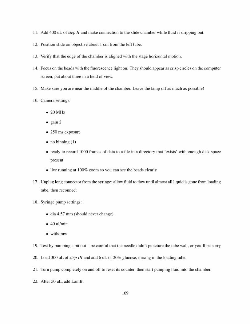
11. Add 400 uL of step II and make connection to the slide chamber while fluid is dripping out.

12. Position slide on objective about 1 cm from the left tube.

13. Verify that the edge of the chamber is aligned with the stage horizontal motion.

14. Focus on the beads with the fluorescence light on. They should appear as crisp circles on the computer

screen; put about three in a field of view.

15. Make sure you are near the middle of the chamber. Leave the lamp off as much as possible!

16. Camera settings:

• 20 MHz

• gain 2

• 250 ms exposure

• no binning (1)

• ready to record 1000 frames of data to a file in a directory that ’exists’ with enough disk space

present

• live running at 100% zoom so you can see the beads clearly

17. Unplug long connector from the syringe; allow fluid to flow until almost all liquid is gone from loading

tube, then reconnect

18. Syringe pump settings:

• dia 4.57 mm (should never change)

• 40 ul/min

• withdraw

19. Test by pumping a bit out—be careful that the needle didn’t puncture the tube wall, or you’ll be sorry

20. Load 300 uL of step III and add 6 uL of 20% glucose, mixing in the loading tube.

21. Turn pump completely on and off to reset its counter, then start pumping fluid into the chamber.

22. After 50 uL, add LamB.

109

23. Turn on fluorescence.

24. Quickly focus on the beads and begin acquisition within 30 s.

25. Watch carefully and adjust focus as necessary during acquisition. Your background should be less

than 180.

26. After movie, turn up speed to 640, pump through some ethanol to clean.

27. Empty syringe into waste container.

28. Put the loading tube aside and use the other clean one for a second experiment.

29. When you’re done, clean up everything and wipe the objective with lens paper.

30. Clean loading tubes especially well because residual SYBR Gold may stain your next sample prema-

turely!

110

C.12 Real-time in vivo single molecule ejection

This procedure is designed to make it possible to visualize the transfer of DNA from single phage λ particles

into host E. coli cells. The strategy is inspired by the microscopic observations of Mosier-Boss et al. (2003)

and Mangenot et al. (2005), who indicated the possibility that fluorescently stained phages could eject their

DNA into cells.

C.12.1 Materials

• NHS-Cy5 (Amersham) 5% (w/v) in DMSO

• PBS buffer

• TM buffer

• SYBR Gold diluted 1:1000 in PBS (Invitrogen)

• CsCl purified λ virions (unpurified samples contain a number of empty heads or unattached tails.)

• E. coli growing rapidly at an optical density of 0.1

• Gloxy (see Section C.11.)

C.12.2 Procedure

1. Spin-filter phages at 10,000 g 3x, replacing buffer each time with 200 µL PBS.

2. Mix 0.2 µL of Cy5 and 2 µL SYBR Gold 1:1000 with the phage solution (the solution will turn a

bright blue or pink).

3. Incubate at 4◦C in the dark for 2 h.

4. Spin-filter phages at 10,000 g 3x in small Amicon spin columns, replacing buffer each time with

200 µL TM buffer.

5. Under the microscope, check that phages are stained correctly.

6. Mix 10 µL phages with 20 µL TM buffer and 10 µL freshly grown cells at an OD600 of 0.5, allow to

stand 10 min at 4◦C to bind.

111

7. Apply 2 µL of cells to an agarose pad (see Section C.4.)

8. Add 1 µL gloxy to the pad, allowing to dry briefly.

9. Transfer pad to observation dish, cover with a fragment of a coverslip, and observe under the micro-

scope. A stage heater at 37◦C is used to warm the sample so that cells may grow.

112

C.13 TM buffer

TM buffer is

• 50 mM TRIS

• 10 mM MgSO47H2O

• pH 7.4

C.13.1 Procedure (10x)

1. Mix ingredients for 500 mL of 10x concentrated TM (30.3 g TRIS, 12.3 g MgSO47H2O) into a little

less than 400 mL.

2. Adjust pH to 7.4 with HCl.

3. Adjust volume to exactly 500 mL.

4. Vacuum-filter and store at 4◦C.

113

C.14 Tethering DNA fragments

The 12-bp overhang on the right end of the lambda genome has the sequence CCCGCCGCTGGA. We take

advantage of the A at the end of the genome in this protocol by using biotinylated dUTP, which is then

streptavidin-tethered to a microscope coverslip. Biotin-streptavidin tethering is used because it is signif-

icantly more detergent resistant than digoxigenin-antidigoxigenin tethering. Adapted from a protocol by

Robert Bao, 2002.

C.14.1 Materials

• 36 µL 0.5 mg/mL λ DNA

• 2.5 µL 1 mM dUTP-biotin

• 2.5 µL 1 mM dATP

• 2.5 µL 1 mM dGTP

• 2.5 µL 1 mM dCTP

• 8 µL 10x EcoPol buffer

• 2 µL Klenow (exo−)

• water to 80 µL

• various restriction enzymes

• 5 mg/mL streptavidin

• Na buffer

• Mg buffer

• flow chamber

C.14.2 Preparing labeled λ-bio DNA stock

1. Mix water, buffer, DNA, dNTPs, and Klenow, pipetting gently with a wide-mouth tip to mix.

114

2. Incubate at 37◦C, 20 min.

3. Add 3 µL EDTA.

4. Heat to 70◦C, 10 min.

5. Ice, 4 min.

6. Dialyze 1 hour on a Millipore filter disc floating on TNE buffer (shiny side up.)

7. Store frozen at -20◦C.

C.14.3 Cutting the DNA

1. Mix the following:

• 18 µL water

• 2 µL 10x buffer (such as NEbuffer 1)

• 1 µL λ-bio from above

• 0.2 µL restriction enzyme (such as EcoRI)

2. Incubate 37◦C 30 min.

3. Dilute with 80 µL Na buffer.

4. Store frozen or (probably) use immediately.

C.14.4 Tethering the DNA fragment

1. Dilute 1µL streptavidin in 250 µL Mg buffer.

2. Flow streptavidin solution onto chamber, incubate 30 min at room temperature.

3. Wash twice with 400 µL Mg buffer.

4. Flow on digested DNA (from above, in Na buffer.)

5. Wash once with 400 µL Na buffer.

6. Flow on observation buffer and measure length in microscope.

115

C.15 Titering

C.15.1 Background

“Titering” a phage means measuring the concentration of phage in a given solution. In typical laboratory

situations, phage concentrations vary over a huge range, from less than 1/ml to over 1013/ml, and we need

a system that can fairly precisely measure the concentration over this whole range. The way we do it is by

diluting the samples so that we have a few hundred in a tube, then adsorb the phage to bacteria and spread

them on a plate. Bacteria will grow everywhere but be killed off in circles (plaques) surrounding the location

of the few hundred phages: these will appear clear or turbid, with a size that depends dramatically on the

species of phage.

Phage concentrations are measured by the ability to form plaques, i.e., in plaque-forming-units/ml, or

pfu/ml. In general, when doing a titer, you follow a procedure that maximizes this number, so that it

represents the true number of active phage within the sample. Things that you should watch out for (because

they can decrease the plaque count) include: lack of time for phage to bind to cells, lack of receptor sites on

cells, dead cells binding to phage, excessive pipetting or vortexing, etc.

This procedure works almost identically for λ and phi29, with the appropriate choice of host cell for

each phage. Probably it will work for others, too.

C.15.2 Materials

• phage solution to be tested

• small LB agar plates at 37◦

• semi-solid LB agar (LB with 7 g/L agar) + 10 mM MgSO4, melted in the microwave and held at

42–46◦

• 1 ml of rapidly growing cells in LB (for lambda: C600; for phi29: su+44). OD600 should be approx-

imately 0.1. (This is when you can first see the growing cells in a 5 mL tube.)

• 10 mM MgSO4

116

C.15.3 Procedure (repeat for each sample to be titered)

1. Put 1 mL 10mM MgSO4 into eppendorf tubes labeled A, B, maybe C, and if you really need it make

a D.

2. Add 1 µL of phage to A (it is diluted to 10−3 of the original concentration) and gently invert 12 times

to mix.

3. Mix 1 µL of A into B (10−6), etc.

4. Prepare several tubes containing 0.1 mL of cell solution.

5. Put the desired quantities of phage from A, B, and C into the cell tubes. For example, if you ex-

pect to have around 1010/mL, you might try 100, 10, and 1 ul of B. If you have no idea about the

concentration, use 10 µL each of A, B, and C for a good first try.

6. Shake the tubes gently to mix the solution and wait for 30min at room temperature (or on ice?) to

allow phages to adsorb to cells.

7. Meanwhile, label the plates!

8. Add 1 mL of warm, molten agar to each tube, one at a time, and pour each quickly onto a correspond-

ingly labeled warm plate.

9. Swirl to make sure it covers the whole plate and quickly rest it on a horizontal surface.

10. Incubate overnight (37◦C for E. coli) and count plaques.

You will you know you are doing a good job when all of the plaques are exactly the same size; smaller

plaques mixed in with the big ones correspond to phages that had not adsorbed when they were mixed into

the agar.

117

Bibliography

N. L. Abbot, D. Blankschtein, and T. A. Hatton. Protein partitioning in two-phase aqueous polymer systems.

2. On the free energy of mixing globular colloids and flexible polymers. Macromolecules, 25(15):3917–

31, 1992.

I. Ali, D. Marenduzzo, and J. M. Yeomans. Dynamics of polymer packaging. J Chem Phys, 121(17):

8635–41, 2004.

D. Anderson. Personal communication, 2005.

J. Arsuaga, R. K. Tan, M. Vazquez, D. W. Sumners, and S. C. Harvey. Investigation of viral DNA packaging

using molecular mechanics models. Biophys Chem, 101:475–84, 2002.

H. P. Babcock, C. Chen, and X. Zhuang. Using single-particle tracking to study nuclear trafficking of viral

genes. Biophys J, 87(4):2749–58, 2004.

J. Benjamin, B. K. Ganser-Pornillos, W. F. Tivol, W. I. Sundquist, and G. J. Jensen. Three-dimensional

structure of HIV-1 virus-like particles by electron cryotomography. J Mol Biol, 346(2):577–88, 2005.

S. Benzer. Fine structure of a genetic region in bacteriophage. Proc Natl Acad Sci U S A, 41(6):344–54,

1955.

G. Bertani. Personal communication, 2005.

B. W. Birren, M. I. Simon, and E. Lai. The basis of high resolution separation of small DNAs by asymmetric-

voltage field inversion electrophoresis and its application to DNA sequencing gels. Nucleic Acids Res, 18

(6):1481–87, 1990.

D. Boal. Mechanics of the Cell. Cambridge University Press, Cambridge, UK, 2002.

C. Canaria and E. Bearer. Personal communication, 2007.

118

G. Cardone, D. C. Winkler, B. L. Trus, N. Cheng, J. E. Heuser, W. W. Newcomb, J. C. Brown, and A. C.

Steven. Visualization of the herpes simplex virus portal in situ by cryo-electron tomography. Virology,

361(2):426–34, 2007.

M. E. Cerritelli, B. Cheng, A. H. Rosenberg, C. E. McPherson, F. P. Booy, and A. C. Steven. Encapsidated

conformation of bacteriophage T7 DNA. Cell, 91:271–80, 1997.

J. Chang, P. Weigele, J. King, W. Chiu, and W. Jiang. Cryo-EM asymmetric reconstruction of bacteriophage

P22 reveals organization of its DNA packaging and infecting machinery. Structure, 14(6):1073–82, 2006.

F. H. Crick, L. Barnett, S. Brenner, and R. J. Watts-Tobin. General nature of the genetic code for proteins.

Nature, 192:1227–32, 1961.

E. K. Davydova, K. M. Kazmierczak, and L. B. Rothman-Denes. Bacteriophage N4-coded, virion-

encapsulated DNA-dependent RNA polymerase. Methods Enzymol, 370:83–94, 2003.

C. Delamarche, D. Thomas, J. P. Rolland, A. Froger, J. Gouranton, M. Svelto, P. Agre, and G. Calamita.

Visualization of AqpZ-mediated water permeability in Escherichia coli by cryoelectron microscopy. J

Bacteriol, 181(14):4193–7, 1999.

T. Dokland and H. Murialdo. Structural transitions during maturation of bacteriophage lambda capsids. J

Mol Biol, 233(4):682–94, 1993.

P. S. Doyle, B. Ladoux, and J. L. Viovy. Dynamics of a tethered polymer in shear flow. Phys Rev Lett, 84

(20):4769–72, 2000.

P. Dufner, L. Jermutus, and R. R. Minter. Harnessing phage and ribosome display for antibody optimisation.

Trends Biotechnol, 24(11):523–9, 2006.

W. C. Earnshaw and S. C. Harrison. DNA arrangement in isometric phage heads. Nature, 268(5621):

598–602, 1977.

A. Evilevitch, L. Lavelle, C. M. Knobler, E. Raspaud, and W. M. Gelbart. Osmotic pressure inhibition of

DNA ejection from phage. PNAS, 100:9292–5, 2003.

A. Evilevitch, M. Castelnovo, C. M. Knobler, and W. M. Gelbart. Measuring the force ejecting DNA from

phage. Journal of Physical Chemistry B, 108(21):6838–43, 2004.

119

A. Evilevitch, J. W. Gober, M. Phillips, C. M. Knobler, and W. M. Gelbart. Measurements of DNA lengths

remaining in a viral capsid after osmotically suppressed partial ejection. Biophysical Journal, 88(1):

751–6, 2005a.

A. Evilevitch, C. M. Knobler, and W. M. Gelbart. Personal communication, 2005b.

M. Feiss, R. A. Fisher, M. A. Crayton, and C. Egner. Packaging of the bacteriophage λ chromosome: Effect

of chromosome length. Virology, 77:281–93, 1977.

J. Filee, F. Tetart, C. A. Suttle, and H. M. Krisch. Marine T4-type bacteriophages, a ubiquitous component

of the dark matter of the biosphere. Proc Natl Acad Sci U S A, 102(35):12471–6, 2005.

R. Fisher, S. Perkins, A. Walker, and E. Wolfart. Spatial filters—laplacian/laplacian of gaussian.

http://homepages.inf.ed.ac.uk/rbf/HIPR2/, 2003.

R. E. Franklin and R. G. Gosling. The structure of sodium thymonucleate fibres. I. The influence of water

content. Acta Cryst, 6:678–685, 1953.

J. A. Fuhrman. Marine viruses and their biogeochemical and ecological effects. Nature, 399(6736):541–8,

1999.

D. Fuller and D. Smith. Personal communication, 2007.

D. N. Fuller, J. P. Rickgauer, S. Grimes, P. J. Jardine, D. L. Anderson, and D. E. Smith. Ionic effects on viral

DNA packaging and portal motor function in bacteriophage φ29. In preparation, 2007.

I. S. Gabashvili and A. Grosberg. Bacteriophage DNA reptation. Biofizika, 36(5):788–93, 1991.

I. S. Gabashvili and A. Grosberg. Dynamics of double stranded DNA reptation from bacteriophage. J

Biomol Struct Dyn, 9(5):911–20, 1992.

L. Gan. Personal communication, 2006.

H. G. Garcia, P. Grayson, L. Han, M. Inamdar, J. Kondev, P. C. Nelson, R. Phillips, J. Widom, and P. A.

Wiggins. Biological consequences of tightly bent DNA: The other life of a macromolecular celebrity.

Biopolymers, 85(2):115–30, 2007.

L. R. Garcia and I. J. Molineux. Rate of translocation of bacteriophage T7 DNA across the membranes of

Escherichia coli. J Bacteriol, 177(14):4066–76, 1995.

120

V. Gonzalez-Huici, M. Salas, and J. M. Hermoso. The push-pull mechanism of bacteriophage φ29 DNA

injection. Molecular Microbiology, 52(2):529–540, 2004.

L. Goodridge, J. Chen, and M. Griffiths. Development and characterization of a fluorescent-bacteriophage

assay for detection of Escherichia coli O157:H7. Appl Environ Microbiol, 65(4):1397–404, 1999.

A. Graff, M. Sauer, P. V. Gelder, and W. Meier. Virus-assisted loading of polymer nanocontainer. Proc Natl

Acad Sci U S A, 99(8):5064–8, 2002.

P. Grayson and I. J. Molineux. Is phage DNA “injected” into cells - biologists and physicists can agree. To

appear in Current Opinion in Microbiology, 2007.

P. Grayson, A. Evilevitch, M. M. Inamdar, P. K. Purohit, W. M. Gelbart, C. M. Knobler, and R. Phillips. The

effect of genome length on ejection forces in bacteriophage lambda. Virology, 348(2):430–6, 2006.

P. Grayson, T. Winther, L. Han, and R. Phillips. The speed of a genome exiting a bacteriophage: real time

observations of lambda DNA ejection in vitro. Submitted to Proc Nat Acad Sci, 2007.

P. J. Hagerman. Flexibility of DNA. Annu. Rev. Biophys. Biophys. Chem., 17:265–86, 1988.

L. Han, S. Blumberg, and R. Phillips. Tethered particle method something. In preparation, 2007.

R. W. Hendrix. Hot new virus, deep connections. Proc Natl Acad Sci U S A, 101(20):7495–6, 2004.

A. D. Hershey and M. Chase. Independent functions of viral protein and nucleic acid in growth of bacterio-

phage. J Gen Physiol, 36(1):39–56, 1952.

S. D. Hicks and C. L. Henley. Irreversible growth model for virus capsid assembly. Phys Rev E Stat Nonlin

Soft Matter Phys, 74(3 Pt 1):031912, 2006.

K. Homma, S. Fukuchi, Y. Nakamura, T. Gojobori, and K. Nishikawa. Gene cluster analysis method iden-

tifies horizontally transferred genes with high reliability and indicates that they provide the main mecha-

nism of operon gain in 8 species of gamma-proteobacteria. Mol Biol Evol, 24(3):805–13, 2007.

S. Huang, S. J. Hayes, and P. Serwer. Fluorescence microscopy of single viral capsids. J Struct Biol, 135

(3):270–80, 2001.

121

J. F. Hubert, L. Duchesne, C. Delamarche, A. Vaysse, H. Gueun, and C. Raguenes-Nicol. Pore selectivity

analysis of an aquaglyceroporin by stopped-flow spectrophotometry on bacterial cell suspensions. Biol

Cell, 97(9):675–86, 2005.

T. Hugel, J. Michaelis, C. L. Hetherington, P. J. Jardine, S. Grimes, J. M. Walter, W. Falk, D. L. Anderson,

and C. Bustamante. Experimental test of connector rotation during DNA packaging into bacteriophage

ϕ29 capsids. PLoS Biol, 5(3):e59, 2007.

M. M. Inamdar, W. M. Gelbart, and R. Phillips. Dynamics of DNA ejection from bacteriophage. Biophys J,

91(2):411–20, 2006.

W. Jiang, J. Chang, J. Jakana, P. Weigele, J. King, and W. Chiu. Structure of epsilon15 bacteriophage reveals

genome organization and DNA packaging/injection apparatus. Nature, 439(7076):612–6, 2006.

I. Katsura. Tail assembly and injection. In R. W. Hendrix, J. W. Roberts, F. W. Stahl, and R. A. Weisberg,

editors, Lambda II, pages 331–346. Cold Spring Harbor, N.Y., 1983.

P. Kemp, M. Gupta, and I. J. Molineux. Bacteriophage T7 DNA ejection into cells is initiated by an enzyme-

like mechanism. Molecular Microbiology, 53(4):1251–65, 2004.

J. Kindt, S. Tzlil, A. Ben-Shaul, and W. M. Gelbart. DNA packaging and ejection forces in bacteriophage.

Proc Natl Acad Sci USA, 98(24):13671–4, 2001.

G. Knaysi. Elements of bacterial cytology, pages 155–67. Comstack Publishing Company, Inc., Ithaca, NY,

2nd edition, 1951.

J. Koehler and R. Phillips. Personal communication, 2005.

R. Koning, S. van den Worm, J. R. Plaisier, J. van Duin, J. P. Abrahams, and H. Koerten. Visualization by

cryo-electron microscopy of genomic RNA that binds to the protein capsid inside bacteriophage MS2. J

Mol Biol, 332(2):415–22, 2003.

T. G. Ksiazek, D. Erdman, C. S. Goldsmith, S. R. Zaki, T. Peret, S. Emery, S. Tong, C. Urbani, J. A. Comer,

W. Lim, P. E. Rollin, S. F. Dowell, A. E. Ling, C. D. Humphrey, W. J. Shieh, J. Guarner, C. D. Paddock,

P. Rota, B. Fields, J. DeRisi, J. Y. Yang, N. Cox, J. M. Hughes, J. W. LeDuc, W. J. Bellini, and L. J.

Anderson. A novel coronavirus associated with severe acute respiratory syndrome. N Engl J Med, 348

(20):1953–66, 2003.

122

J. C. LaMarque, T. V. Le, and S. C. Harvey. Packaging double-helical DNA into viral capsids. Biopolymers,

73(3):348–55, 2004.

G. C. Lander, L. Tang, S. R. Casjens, E. B. Gilcrease, P. Prevelige, A. Poliakov, C. S. Potter, B. Carragher,

and J. E. Johnson. The structure of an infectious P22 virion shows the signal for headful DNA packaging.

Science, 312(5781):1791–5, 2006.

S. H. Lee, M. Onuki, H. Satoh, and T. Mino. Isolation, characterization of bacteriophages specific to

Microlunatus phosphovorus and their application for rapid host detection. Lett Appl Microbiol, 42(3):

259–64, 2006.

K. N. Lentz, A. D. Smith, S. C. Geisler, S. Cox, P. Buontempo, A. Skelton, J. DeMartino, E. Rozhon,

J. Schwartz, V. Girijavallabhan, J. O’Connell, and E. Arnold. Structure of poliovirus type 2 Lansing

complexed with antiviral agent SCH48973: comparison of the structural and biological properties of

three poliovirus serotypes. Structure, 5(7):961–78, 1997.

L. Letellier, P. Boulanger, L. Plancon, P. Jacquot, and M. Santamaria. Main features on tailed phage, host

recognition and DNA uptake. Frontiers in Bioscience, 9:1228–339, 2004.

D. Lof, K. Schillen, B. Jonsson, and A. Evilevitch. Forces controlling the rate of DNA ejection from phage

lambda. J Mol Biol, 368(1):55–65, 2007.

S. E. Luria and M. Delbruck. Mutations of bacteria from virus sensitivity to virus resistance. Genetics, 28

(6):491–511, 1943.

A. P. Lyubartsev and L. Nordenskiold. Monte carlo simulation study of ion distribution and osmotic pressure

in hexagonally oriented DNA. Journal of Physical Chemistry, 99:10373–82, 1995.

S. Mangenot. Personal communication, 2005.

S. Mangenot, M. Hochrein, J. Rdler, and L. Letellier. Real-time imaging of DNA ejection from single phage

particles. Curr Biol, 15(5):430–5, 2005.

G. Manning. Limiting laws and counterion condensation in polyelectrolyte solutions I. Colligative proper-

ties. J Chem Phys, 51(3):924–33, 1969.

123

D. Marenduzzo and C. Micheletti. Thermodynamics of DNA packaging inside a viral capsid: the role of

DNA intrinsic thickness. J Mol Biol, 330(3):485–92, 2003.

D. Marsh. Scaling and mean-field theories applied to polymer brushes. Biophysical Journal, 86:2630–2633,

2004.

M. McCarty and O. T. Avery. Studies on the chemical nature of the substance inducing transformation

of pneumococcal types: II. Effect of desoxyribonuclease on the biological activity of the transforming

substance. Journal of Experimental Medicine, 83(2):89–96, 1946.

S. Meijer and A. Feenstra. CCMV overview. http://gcg.tran.wau.nl/ccmv-overview/CCMV.html, 11 1998.

B. E. Michel. Evaluation of the water potentials of solutions of polyethylene glycol 8000 both in the absence

and presence of other solutes. Plant Physiology, 72:66–70, 1983.

I. Molineux. No syringes please, ejection of T7 DNA from the virion is enzyme driven. Molecular Micro-

biology, 40(1):1–8, 2001.

M. L. Morse, E. M. Lederberg, and J. Lederberg. Transduction in escherichia coli K-12. Genetics, 41(1):

142–56, 1956.

P. A. Mosier-Boss, S. H. Lieberman, J. M. Andrews, F. L. Rohwer, L. E. Wegley, and M. Breitbart. Use of

fluorescently labeled phage in the detection and identification of bacterial species. Appl Spectrosc, 57(9):

1138–44, 2003.

S. Mukhopadhyay, B. S. Kim, P. R. Chipman, M. G. Rossmann, and R. J. Kuhn. Structure of west nile virus.

Science, 302(5643):248, 2003.

N. E. Murray and K. Murray. Manipulation of restriction targets in phage lambda to form receptor chromo-

somes for DNA fragments. Nature, 251(5475):476–81, 1974.

F. Neidhardt, editor. Escherichia Coli and Salmonella Typhimurium. ASM Press, Washington, DC, 1996.

W. Newcomb. Personal communication, 2006.

H. B. Newcombe. Origin of bacterial variants. Nature, 164(4160):150–1, 1949.

S. L. Novick and J. D. Baldeschweiler. Fluorescence measurement of the kinetics of DNA injection by

bacteriophage λ into liposomes. Biochemistry, 27:7919–24, 1988.

124

M. Oda, M. Morita, H. Unno, and Y. Tanji. Rapid detection of Escherichia coli O157:H7 by using green

fluorescent protein-labeled PP01 bacteriophage. Appl Environ Microbiol, 70(1):527–34, 2004.

T. Odijk. Hexagonally packed DNA within bacteriophage T7 stabilized by curvature stress. Biophys. J., 75

(3):1223–7, 1998.

T. Odijk. Statics and dynamics of condensed DNA within phages and globules. Philos Transact A Math

Phys Eng Sci, 362(1820):1497–517, 2004.

Y. A. O’Shea and E. F. Boyd. Mobilization of the Vibrio pathogenicity island between Vibrio cholerae

isolates mediated by CP-T1 generalized transduction. FEMS Microbiol Lett, 214(2):153–7, 2002.

M. D. Paepe and F. Taddei. Viruses’ life history: Towards a mechanistic basis of a trade-off between survival

and reproduction among phages. PLoS Biol, 4(7):e193, 2006.

J. S. Parkinson and R. J. Huskey. Deletion mutants of bacteriophage lambda. I. Isolation and initial charac-

terization. J Mol Biol, 56(2):369–84, 1971.

V. A. Parsegian, R. P. Rand, N. L. Fuller, and D. C. Rau. Osmotic stress for the direct measurement of

intermolecular forces. Methods in Enzymology, 127:400–16, 1986.

R. Podgornik, H. H. Strey, D. C. Rau, and V. A. Parsegian. Watching molecules crowd: DNA double helices

under osmotic stress. Biophys Chem, 57(1):111–21, 1995.

R. R. Pollitzer. Cholera studies. V. Bacteriophage investigations. Bull World Health Organ, 13(1):1–25,

1955.

M. Ptashne. A Genetic Switch. Blackwell, Oxford, United Kingdom, 1992.

P. K. Purohit, J. Kondev, and R. Phillips. Mechanics of DNA packaging in viruses. PNAS, 100:3173–8,

2003.

P. K. Purohit, M. M. Inamdar, P. D. Grayson, T. M. Squires, J. Kondev, and R. Phillips. Forces during

bacteriophage DNA packaging and ejection. Biophysical Journal, 2005. In press.

A. Rambach and P. Tiollais. Bacteriophage lambda having EcoRI endonuclease sites only in the nonessential

region of the genome. Proc Natl Acad Sci U S A, 71(10):3927–30, 1974.

125

D. Raoult, S. Audic, C. Robert, C. Abergel, P. Renesto, H. Ogata, B. L. Scola, M. Suzan, and J. M. Claverie.

The 1.2-megabase genome sequence of Mimivirus. Science, 306(5700):1344–50, 2004.

D. C. Rau, B. Lee, and V. A. Parsegian. Measurement of the repulsive force between polyelectrolyte

molecules in ionic solution: hydration forces between parallel DNA double helices. PNAS, 81(9):2621–5,

1984.

G. Rice, L. Tang, K. Stedman, F. Roberto, J. Spuhler, E. Gillitzer, J. E. Johnson, T. Douglas, and M. Young.

The structure of a thermophilic archaeal virus shows a double-stranded DNA viral capsid type that spans

all domains of life. Proc Natl Acad Sci U S A, 101(20):7716–20, 2004.

S. C. Riemer and V. A. Bloomfield. Packaging of DNA in bacteriophage heads: some considerations on

energetics. Biopolymers, 17(3):785–94, 1978.

F. Rohwer. Global phage diversity. Cell, 113(2):141, 2003.

M. Rubinstein and A. Grosberg. Personal communication, 2007.

M. J. Rust, M. Lakadamyali, F. Zhang, and X. Zhuang. Assembly of endocytic machinery around individual

influenza viruses during viral entry. Nat Struct Mol Biol, 11(6):567–73, 2004.

C. Sao-Jose, C. Baptista, and M. A. Santos. Bacillus subtilis operon encoding a membrane receptor for

bacteriophage SPP1. J Bacteriol, 186(24):8337–46, 2004.

P. F. Seaman and M. J. Day. Isolation and characterization of a bacteriophage with an unusually large

genome from the Great Salt Plains National Wildlife Refuge, Oklahoma, USA. FEMS Microbiol Ecol,

60(1):1–13, 2007.

D. Smith, S. Tans, S. Smith, S. Grimes, D. Anderson, and C. Bustamante. The bacteriophage phi29 portal

motor can package DNA against a large internal force. Nature, 413:748–52, 2001.

A. J. Spakowitz and Z. G. Wang. DNA packaging in bacteriophage: is twist important? Biophys J, 88(6):

3912–23, 2005.

J. A. Speir, S. Munshi, G. Wang, T. S. Baker, and J. E. Johnson. Structures of the native and swollen forms

of cowpea chlorotic mottle virus determined by X-ray crystallography and cryo-electron microscopy.

Structure, 3(1):63–78, 1995.

126

J. B. Stock, B. Rauch, and S. Roseman. Periplasmic space in Salmonella typhimurium and Escherichia coli.

J Biol Chem, 252(21):7850–61, 1977.

H. H. Strey, V. A. Parsegian, and R. Podgornik. Equation of state for DNA liquid crystals: Fluctuation

enhanced electrostatic double layer repulsion. Phys Rev Lett, 78(5):895, 1997.

H. H. Strey, R. Podgornik, D. C. Rau, and V. A. Parsegian. DNA–DNA interactions. Curr Opin Struct Biol,

8(3):309–13, 1998.

Y. Tao, N. H. Olson, W. Xu, D. L. Anderson, M. G. Rossmann, and T. S. Baker. Assembly of a tailed

bacterial virus and its genome release studied in three dimensions. Cell, 95(3):431–7, 1998.

M. Thomas, J. R. Cameron, and R. W. Davis. Viable molecular hybrids of bacteriophage lambda and

eukaryotic DNA. Proc Natl Acad Sci U S A, 71(11):4579–83, 1974.

P. Tiollais, M. Perricaudet, U. Pettersson, and L. Philipson. Propagation in E. coli of bacteriophage lambda

with integrated fragments of adenovirus 2 DNA. Gene, 1(1):49–63, 1976.

S. Tzlil, J. T. Kindt, W. M. Gelbart, and A. Ben-Shaul. Forces and pressures in DNA packaging and release

from viral capsids. Biophysical Journal, 84(3):1616–27, 2003.

J. D. Watson and F. H. Crick. Molecular structure of nucleic acids; a structure for deoxyribose nucleic acid.

Nature, 171(4356):737–8, 1953.

E. Weisstein. Laminar flow. http://scienceworld.wolfram.com/physics/LaminarFlow.html, 2005.

World Health Organization. Smallpox. http://www.who.int/mediacentre/factsheets/smallpox/en/, 2007.

A. Yildiz, J. N. Forkey, S. A. McKinney, T. Ha, Y. E. Goldman, and P. R. Selvin. Myosin V walks hand-

over-hand: single fluorophore imaging with 1.5-nm localization. Science, 300(5628):2061–5, 2003.

R. Zandi, D. Reguera, R. F. Bruinsma, W. M. Gelbart, and J. Rudnick. Origin of icosahedral symmetry in

viruses. Proc Natl Acad Sci U S A, 101(44):15556–60, 2004.

V. Zarybnicky. Mechanism of T-even DNA ejection. J Theor Biol, 22(1):33–42, 1969.

C. Zurla, A. Franzini, G. Galli, D. Dunlap, D. Lewis, S. Adhya, and L. Finzi. Novel tethered particle motion

analysis of CI protein-mediated DNA looping in the regulation of bacteriophage lambda. Journal of

Physics: Condensed Matter, 18(14):S225–34, 2006.

127