the donaldson-thomas theory of via the …jbryan/papers/k3xe.pdf · the donaldson-thomas theory of...

THE DONALDSON-THOMAS THEORY OF K3× E VIA THETOPOLOGICAL VERTEX.

JIM BRYAN

ABSTRACT. We give a general overview of the Donaldson-Thomas invariants of ellipticfibrations and their relation to Jacobi forms. We then focus on the specific case of where thefibration is S×E, the product of aK3 surface and an elliptic curve. Oberdieck and Pand-haripande conjectured [11] that the partition function of the Gromov-Witten/Donaldson-Thomas invariants of S × E is given by minus the reciprocal of the Igusa cusp form ofweight 10. For a fixed primitive curve class in S of square 2h − 2, their conjecture pre-dicts that the corresponding partition functions are given by meromorphic Jacobi forms ofweight −10 and index h − 1. We calculate the Donaldson-Thomas partition function forprimitive classes of square -2 and of square 0, proving strong evidence for their conjecture.

Our computation uses reduced Donaldson-Thomas invariants which are defined as the(Behrend function weighted) Euler characteristics of the quotient of the Hilbert schemeof curves in S × E by the action of E. Our technique is a mixture of motivic and toricmethods (developed with Kool in [4]) which allows us to express the partition functions interms of the topological vertex and subsequently in terms of Jacobi forms. We computeboth versions of the invariants: unweighted and Behrend function weighted Euler charac-teristics. Our Behrend function weighted computation requires us to assume Conjecture18 in [4].

1. AN OVERVIEW OF DONALDSON-THOMAS THEORY FOR ELLIPTIC FIBRATIONS.

Let X be a quasi-projective non-singular Calabi-Yau threefold over C. The Donaldson-Thomas invariants are a virtual count of sheaves on X . They are invariant under defor-mations and they are the mathematical counterpart of counting BPS states in type IIBtopological string theory compactified on X . Of particular importance is the case wherethe sheaves are ideal sheaves of curves. Then the Donaldson-Thomas invariants “countcurves”, encoding subtle information about the enumerative geometry of X .

We can identify the moduli space of ideal sheaves of curves with

Hilbβ,n(X) = {Z ⊂ X : [Z] = β ∈ H2(X), n = χ(OZ)}

the Hilbert scheme of proper subschemes ofX with fixed homology class and holomorphicEuler characteristic. To obtain a curve count, we would like to determine the “number ofpoints” in Hilbβ,n(X). One way to assign an integer to a C-scheme, which generalizes thenumber of points in a zero dimensional scheme, is the topological Euler characteristic ofthe scheme with its complex analytic topology. This gives rise to the “naıve Donaldson-Thomas invariant” which we denote by

DT β,n(X) = e(Hilbβ,n(X)).

Date: January 30, 2018.1

2 JIM BRYAN

The term “invariant” is somewhat of a misnomer for this quantity since in general, it is notinvariant under deformations1 of X .

Topological Euler characteristic is insensitive to the singularities and non-reduced struc-ture of the Hilbert scheme and to get a true deformation invariant, these must be taken intoaccount. Instead, we define the Donaldson-Thomas invariant as a weighted Euler charac-teristic:

DTβ,n(X) =∑k∈Z

k · e(ν−1(k))

whereν : Hilbβ,n(X)→ Z

is the Behrend function. The Behrend function is an integer-valued constructible func-tion, defined for any C-scheme, which is sensitive to non-reducedness and singularities.Behrend proves [1] that this definition of DTβ,n(X) agrees with the traditional definitiongiven by the degree of the virtual fundamental class [10], which is a deformation invariant2.

It will be notationally convenient to treat an Euler characteristic weighted by a con-structible function as a Lebesgue integral, where the measurable sets are constructible sets,the measurable functions are constructible functions, and the measure of a set is given byits Euler characteristic. In this language, one writes

DTβ,n(X) =

∫Hilbβ,n(X)

ν de.

In general, Donaldson-Thomas invariants are extremely hard to compute. However, theconnection to physics, has provided several conjectures suggesting that the invariants havea rich structure. A particularly beautiful instance of this is a conjecture of Huang, Katz,and Klemm [9] (see also [8]) which can be roughly expressed as the following slogan:

Generating functions for the Donaldson-Thomas invariants of ellipti-cally fibered Calabi-Yau threefolds are given by the Fourier expansionsof Jacobi forms.

To give more details, suppose that X is elliptically fibered, that is π : X → S is a flatfamily of genus one curves over a smooth surface S with a section σ : S → X . For a curveclass β in S, we let

β + dE ∈ H2(X)

be the curve class given by σ∗(β) + d[π−1(pt)], that is a class in the base plus d times thefiber class. We define a partition function

ZDTβ (X) =

∑n,d

DTβ+dE,n(X) qd+12KS ·β (−p)n.

Then the Huang-Katz-Klemm conjecture is

Conjecture 1.1. Let S be Fano3 and let h be the arithmetic genus of β. Then

ZDTβ (X)

ZDT0 (X)

1Although, from general considerations, DTβ,n(X) is a constructible function on the deformation space ofX and hence it is an invariant of the generic member of each deformation type.

2The traditional definition is only for projective X . When X is only quasi-projective, the weighted Eulercharacteristic definition is well defined, but no longer guarenteed to be a deformation invariant.

3It is not clear what the optimal hypotheses on π : X → S should be. In [9], they primary consider thecase of Fano S and where all fibers π−1(pt) are irreducible, but they discuss other cases, including the trivialfibrations studied in this paper.

THE DONALDSON-THOMAS THEORY OF K3× E VIA THE TOPOLOGICAL VERTEX. 3

is a Jacobi form of index h− 1 and weight l = l(S, β) and with variables

q = exp (2πiτ) , p = exp (2πiz) .

We make several remarks:• A Jacobi form is a two variable generization of modular forms which depend on

both a modular parameter τ ∈ H and an elliptic parameter z ∈ C. Jacobi forms aremeromorphic functions on H× C satisfying a modular transformation law underthe action of SL2(Z) and an elliptic transformation law under lattice translations(see [7]).

• The denominator in the conjecture is ZDT0 (X) is the partition function for the fiber

class invariants. An explicit expression for this series has been computed by Toda[17].

• This conjecture reveals that the Donaldson-Thomas invariants have a beautifulinternal structure and a suprising connection with number theory. Additionally,the conjecture is a powerful computational tool: since the Jacobi forms of a fixedweight and degree form a finite dimensional vector space, the conjecture reducesan infinite number of computations down to a finite number. In [9], several explicitpredictions are made and partially checked.

• A proof of the elliptic transformation law was given by Oberdieck and Shen usinga fiberwise Fourier-Mukai transform and wall-crossing techniques [14]. Oberdieckand Shen were able to use their result to confirm several cases of the Huang-Katz-Klemm conjecture.

• The variable change p = exp (2πiz) is close to the variable change p = exp (iλ)which (conjecturally) equates the Donaldson-Thomas partition function to theGromov-Witten partition function[10]. So while Donaldson-Thomas invariantsof an elliptically fibered Calabi-Yau threefold are the coefficients of the Fourierexpansion of a Jacobi form, the Gromov-Witten invariants are essentially the co-efficients of the Taylor expansion of the same Jacobi form.

• A proof for a the local version of the conjecture (where X is a local elliptic sur-face), was given in [4].

2. THE CASE OF K3× E: OVERVIEW

In this paper we focus on the simpliest possible elliptically fibered Calabi-Yau threefold,namely where X = S × E where S is a K3 surface and E is an elliptic curve. In [11],Oberdieck and Pandharipande conjectured that the partition function for the curve countinginvariants of X is given by −1/χ10, minus the reciprocal of the weight 10 Igusa cuspform4,5 . The relevant curve counting invariants include modified versions of Gromov-Witten invariants and stable pairs invariants. In this paper, we define modified Donaldson-Thomas invariants of X . Our definition is given by taking the Euler characteristic of thequotient of the Hilbert scheme of curves on X by the action of the elliptic curve (weconsider both the Behrend function weighted and unweighted Euler characteristics). Ourinvariants are expected to be equal to the invariants defined via stable pairs in [11].

4Oberdieck and Pandharipande were the first to formulate a mathematically precise conjecture, but the ap-pearence of the Igusa cusp form in closely related partition functions in physics dates back to the mid-nineties[6].

5Since this paper was originally written in 2015, Oberdieck and Pixton have given a complete proof of thisconjecture using methods (different from ours) from both Donaldson-Thomas theory and Gromov-Witten theory[13].

4 JIM BRYAN

We employ an approach to computing these invariants which uses a mixture of motivicand toric methods (technology developed with M. Kool in [4]). We show that these meth-ods yield complete computations for the partition functions of X in the case where S isK3 surface with a primitive curve class of square−2 or of square 0 (assuming Conj. 18 [4]in the Behrend function weighted case). The resulting partition functions are given by theJacobi forms F−2∆−1 and −24℘∆−1 respectively where F is a Jacobi theta function, ∆is the discriminant modular form, and ℘ is the Weierstrass ℘ function. This agrees with theprediction from by the Oberdieck-Pandharipande conjecture thus proving their conjecturefor primitive curve classes in the K3 of square −2 or 0.

Our general computational strategy is the following. Donaldson-Thomas invariants aregiven by weighted Euler characteristics of Hilbert schemes. We stratify the Hilbert schemeusing the geometric support of the curves and we compute Euler characteristics of strataseparately. Many of the strata acquire actions of E or C∗ (that were not present globally)and we restrict to the fixed point loci. We are able to further stratify the fixed point lociand those strata sometimes acquire further actions. Iterating this strategy, we reduce thecomputation to subschemes which are formally locally given by monomial ideals. Theseare counted using the topological vertex. New identities for the topological vertex lead toclosed formulas. To incorporate the Behrend function into this strategy, we must assumethe conjecture formulated in [4, Conj. 18]. This is a general conjecture regarding thebehavior of the Behrend function at subschemes given locally by monomial ideals.

3. THE CASE OF K3× E: DEFINITIONS, CONJECTURES, AND RESULTS.

As above, letX = S × E

where S is a non-singular K3 surface with a primitive curve class β of square

β2 = 2h− 2.

We call h the genus of the K3 surface. Let

β + dE ∈ H2(X)

denote the class iS∗(β)+iE∗(d[E]) where iS : S → X and iE : E → X are the inclusionsobtained from choosing points s ∈ S and e ∈ E.

It is worth emphasizing:

The ordinary Donaldson-Thomas invariants DTβ+dE,n(X) are all zero.

This can be seen in two different ways:

(1) The action of E on Hilbβ+dE,n(X) is fixed point free, consequently its (Behrendfunction6 weighted) Euler characteristic is zero.

(2) There exists deformations of S which make β non-algebraic. Under this deforma-tion, the Hilbert scheme Hilbβ+dE,n(X) becomes empty. Since DTβ+dE,n(X) isdeformation invariant it must be zero.

Remarkably, the above two issues can be solved simultaneously by taking the weightedEuler characteristic of the quotient of the Hilbert scheme.

6The value of the Behrend function at a closed point of a scheme only depends on the local ring of that point,therefore the Behrend function of a scheme is invariant under any group action.


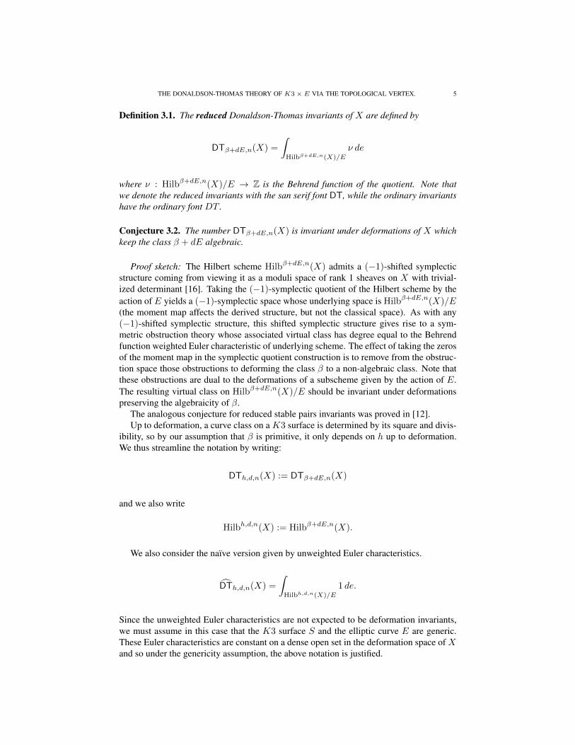
Definition 3.1. The reduced Donaldson-Thomas invariants of X are defined by

DTβ+dE,n(X) =

∫Hilbβ+dE,n(X)/E

ν de

where ν : Hilbβ+dE,n(X)/E → Z is the Behrend function of the quotient. Note thatwe denote the reduced invariants with the san serif font DT, while the ordinary invariantshave the ordinary font DT .

Conjecture 3.2. The number DTβ+dE,n(X) is invariant under deformations of X whichkeep the class β + dE algebraic.

Proof sketch: The Hilbert scheme Hilbβ+dE,n(X) admits a (−1)-shifted symplecticstructure coming from viewing it as a moduli space of rank 1 sheaves on X with trivial-ized determinant [16]. Taking the (−1)-symplectic quotient of the Hilbert scheme by theaction of E yields a (−1)-symplectic space whose underlying space is Hilbβ+dE,n(X)/E(the moment map affects the derived structure, but not the classical space). As with any(−1)-shifted symplectic structure, this shifted symplectic structure gives rise to a sym-metric obstruction theory whose associated virtual class has degree equal to the Behrendfunction weighted Euler characteristic of underlying scheme. The effect of taking the zerosof the moment map in the symplectic quotient construction is to remove from the obstruc-tion space those obstructions to deforming the class β to a non-algebraic class. Note thatthese obstructions are dual to the deformations of a subscheme given by the action of E.The resulting virtual class on Hilbβ+dE,n(X)/E should be invariant under deformationspreserving the algebraicity of β.

The analogous conjecture for reduced stable pairs invariants was proved in [12].Up to deformation, a curve class on a K3 surface is determined by its square and divis-

ibility, so by our assumption that β is primitive, it only depends on h up to deformation.We thus streamline the notation by writing:

DTh,d,n(X) := DTβ+dE,n(X)

and we also write

Hilbh,d,n(X) := Hilbβ+dE,n(X).

We also consider the naıve version given by unweighted Euler characteristics.

DTh,d,n(X) =

∫Hilbh,d,n(X)/E

1 de.

Since the unweighted Euler characteristics are not expected to be deformation invariants,we must assume in this case that the K3 surface S and the elliptic curve E are generic.These Euler characteristics are constant on a dense open set in the deformation space of Xand so under the genericity assumption, the above notation is justified.

6 JIM BRYAN

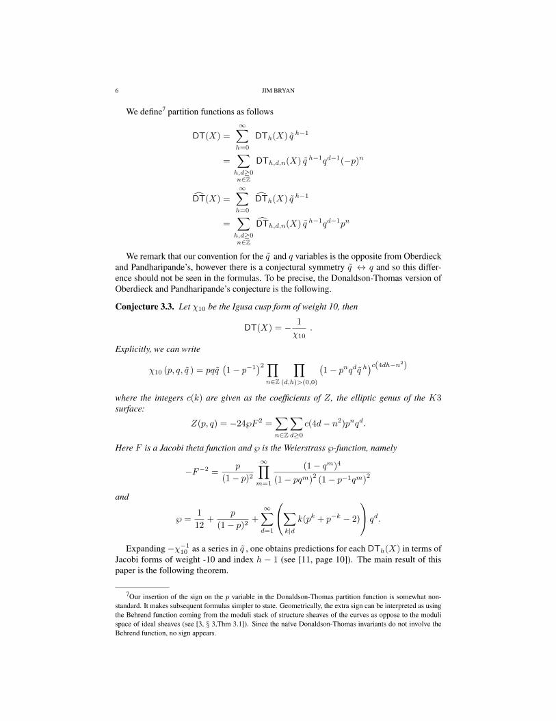
We define7 partition functions as follows

DT(X) =

∞∑h=0

DTh(X) q h−1

=∑h,d≥0n∈Z

DTh,d,n(X) q h−1qd−1(−p)n

DT(X) =

∞∑h=0

DTh(X) q h−1

=∑h,d≥0n∈Z

DTh,d,n(X) q h−1qd−1pn

We remark that our convention for the q and q variables is the opposite from Oberdieckand Pandharipande’s, however there is a conjectural symmetry q ↔ q and so this differ-ence should not be seen in the formulas. To be precise, the Donaldson-Thomas version ofOberdieck and Pandharipande’s conjecture is the following.

Conjecture 3.3. Let χ10 be the Igusa cusp form of weight 10, then

DT(X) = − 1

χ10.

Explicitly, we can write

χ10 (p, q, q ) = pqq(1− p−1

)2 ∏n∈Z

∏(d,h)>(0,0)

(1− pnqdq h

)c(4dh−n2)

where the integers c(k) are given as the coefficients of Z, the elliptic genus of the K3surface:

Z(p, q) = −24℘F 2 =∑n∈Z

∑d≥0

c(4d− n2)pnqd.

Here F is a Jacobi theta function and ℘ is the Weierstrass ℘-function, namely

−F−2 =p

(1− p)2∞∏m=1

(1− qm)4

(1− pqm)2

(1− p−1qm)2

and

℘ =1

12+

p

(1− p)2+

∞∑d=1

∑k|d

k(pk + p−k − 2)

qd.

Expanding −χ−110 as a series in q , one obtains predictions for each DTh(X) in terms ofJacobi forms of weight -10 and index h − 1 (see [11, page 10]). The main result of thispaper is the following theorem.

7Our insertion of the sign on the p variable in the Donaldson-Thomas partition function is somewhat non-standard. It makes subsequent formulas simpler to state. Geometrically, the extra sign can be interpreted as usingthe Behrend function coming from the moduli stack of structure sheaves of the curves as oppose to the modulispace of ideal sheaves (see [3, § 3,Thm 3.1]). Since the naıve Donaldson-Thomas invariants do not involve theBehrend function, no sign appears.


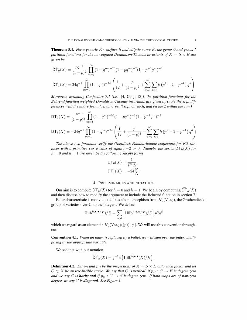
Theorem 3.4. For a generic K3 surface S and elliptic curve E, the genus 0 and genus 1partition functions for the unweighted Donaldson-Thomas invariants of X = S × E aregiven by

DT0(X) =pq−1

(1− p)2∞∏m=1

(1− qm)−20(1− pqm)−2(1− p−1qm)−2

DT1(X) = 24q−1∞∏m=1

(1− qm)−24

1

12+

p

(1− p)2+

∞∑d=1

∑k|d

k(pk + 2 + p−k

)qd

Moreover, assuming Conjecture 7.1 (i.e. [4, Conj. 18]), the partition functions for theBehrend function weighted Donaldson-Thomas invariants are given by (note the sign dif-ferences with the above formulae, an overall sign on each, and on the 2 within the sum)

DT0(X) =−pq−1

(1− p)2∞∏m=1

(1− qm)−20(1− pqm)−2(1− p−1qm)−2

DT1(X) = −24q−1∞∏m=1

(1− qm)−24

1

12+

p

(1− p)2+

∞∑d=1

∑k|d

k(pk − 2 + p−k

)qd

The above two formulas verify the Oberdieck-Pandharipande conjecture for K3 sur-

faces with a primitive curve class of square −2 or 0. Namely, the series DTh(X) forh = 0 and h = 1 are given by the following Jacobi forms

DT0(X) =1

F 2∆,

DT1(X) = −24℘

∆.

4. PRELIMINARIES AND NOTATION.

Our aim is to compute DTh(X) for h = 0 and h = 1. We begin by computing DTh(X)and then discuss how to modify the argument to include the Behrend function in section 7.

Euler characteristic is motivic: it defines a homomorphism fromK0(VarC), the Grothendieckgroup of varieties over C, to the integers. We define

Hilbh,•,•(X)/E =∑n,d

[Hilbh,d,n(X)/E

]pnqd

which we regard as an element inK0(VarC)((p))[[q]]. We will use this convention through-out:

Convention 4.1. When an index is replaced by a bullet, we will sum over the index, multi-plying by the appropriate variable.

We see that with our notation

DTh(X) = q−1e(

Hilbh,•,•(X)/E).

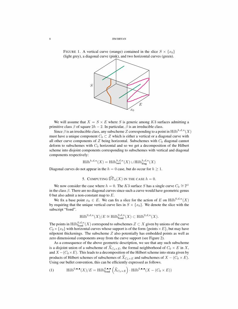
Definition 4.2. Let pS and pE be the projections of X = S × E onto each factor and letC ⊂ X be an irreducible curve. We say that C is vertical if pE : C → E is degree zeroand we say C is horizontal if pS : C → S is degree zero. If both maps are of non-zerodegree, we say C is diagonal. See Figure 1.

8 JIM BRYAN

FIGURE 1. A vertical curve (orange) contained in the slice S × {x0}(light grey), a diagonal curve (pink), and two horizontal curves (green).

S

E

x0

We will assume that X = S × E where S is generic among K3 surfaces admitting aprimitive class β of square 2h− 2. In particular, β is an irreducible class.

Since β is an irreducible class, any subschemeZ corresponding to a point in Hilbh,d,n(X)must have a unique component C0 ⊂ Z which is either a vertical or a diagonal curve withall other curve components of Z being horizontal. Subschemes with C0 diagonal cannotdeform to subschemes with C0 horizontal and so we get a decomposition of the Hilbertscheme into disjoint components corresponding to subschemes with vertical and diagonalcomponents respectively:

Hilbh,d,n(X) = Hilbh,d,nvert (X) tHilbh,d,ndiag (X)

Diagonal curves do not appear in the h = 0 case, but do occur for h ≥ 1.

5. COMPUTING DTh(X) IN THE CASE h = 0.

We now consider the case where h = 0. The K3 surface S has a single curve C0∼= P1

in the class β. There are no diagonal curves since such a curve would have geometric genus0 but also admit a non-constant map to E.

We fix a base point x0 ∈ E. We can fix a slice for the action of E on Hilb0,d,n(X)by requiring that the unique vertical curve lies in S × {x0}. We denote the slice with thesubscript “fixed”.

Hilb0,d,n(X)/E ∼= Hilb0,d,nfixed (X) ⊂ Hilb0,d,n(X).

The points in Hilb0,d,nfixed (X) correspond to subschemes Z ⊂ X given by unions of the curve

C0×{x0} with horizontal curves whose support is of the form {points×E}, but may havenilpotent thickenings. The subscheme Z also potentially has embedded points as well aszero dimensional components away from the curve support (see Figure 2).

As a consequence of the above geometric description, we see that any such subschemeis a disjoint union of a subscheme of XC0×E , the formal neighborhood of C0 × E in X ,andX−(C0×E). This leads to a decomposition of the Hilbert scheme into strata given byproducts of Hilbert schemes of subschemes of XC0×E and subschemes of X − (C0 ×E).Using our bullet convention, this can be efficiently expressed as follows.

(1) Hilb0,•,•(X)/E = Hilb0,•,•fixed

(XC0×E

)·Hilb0,•,•(X − (C0 × E))


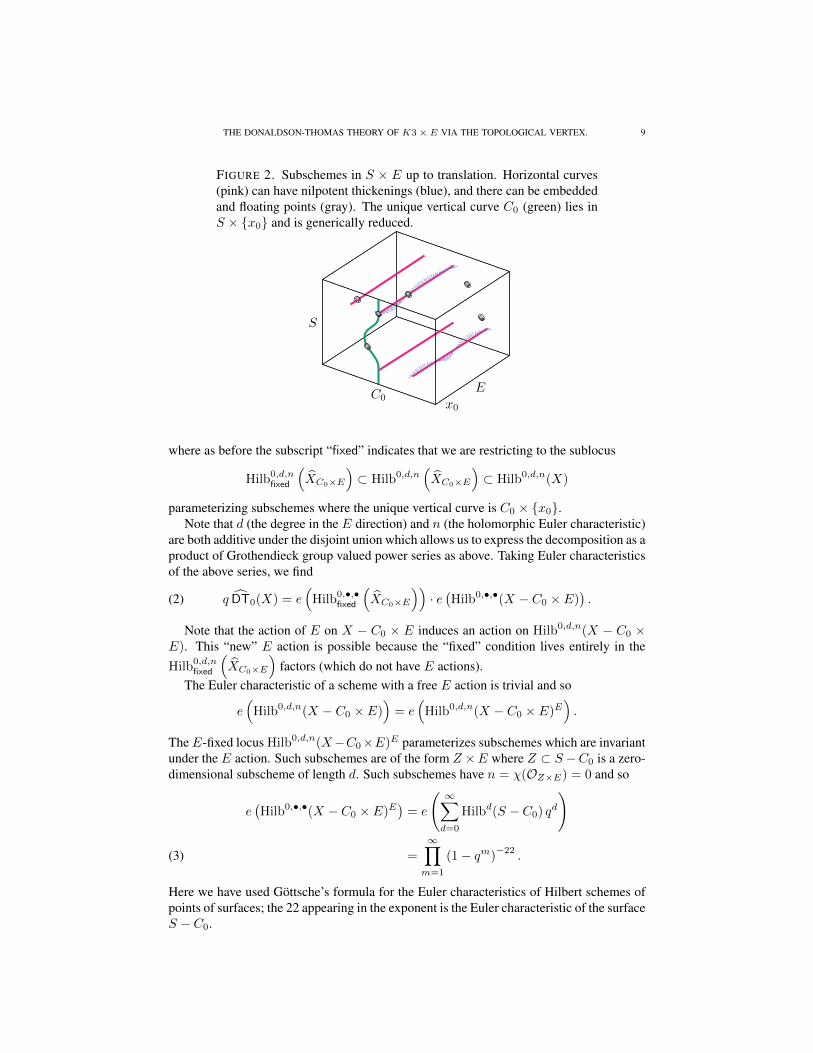
FIGURE 2. Subschemes in S × E up to translation. Horizontal curves(pink) can have nilpotent thickenings (blue), and there can be embeddedand floating points (gray). The unique vertical curve C0 (green) lies inS × {x0} and is generically reduced.

S

E

x0C0

where as before the subscript “fixed” indicates that we are restricting to the sublocus

Hilb0,d,nfixed

(XC0×E

)⊂ Hilb0,d,n

(XC0×E

)⊂ Hilb0,d,n(X)

parameterizing subschemes where the unique vertical curve is C0 × {x0}.Note that d (the degree in the E direction) and n (the holomorphic Euler characteristic)

are both additive under the disjoint union which allows us to express the decomposition as aproduct of Grothendieck group valued power series as above. Taking Euler characteristicsof the above series, we find

(2) q DT0(X) = e(

Hilb0,•,•fixed

(XC0×E

))· e(Hilb0,•,•(X − C0 × E)

).

Note that the action of E on X − C0 × E induces an action on Hilb0,d,n(X − C0 ×E). This “new” E action is possible because the “fixed” condition lives entirely in theHilb0,d,n

fixed

(XC0×E

)factors (which do not have E actions).

The Euler characteristic of a scheme with a free E action is trivial and so

e(

Hilb0,d,n(X − C0 × E))

= e(

Hilb0,d,n(X − C0 × E)E).

TheE-fixed locus Hilb0,d,n(X−C0×E)E parameterizes subschemes which are invariantunder the E action. Such subschemes are of the form Z ×E where Z ⊂ S −C0 is a zero-dimensional subscheme of length d. Such subschemes have n = χ(OZ×E) = 0 and so

e(Hilb0,•,•(X − C0 × E)E

)= e

( ∞∑d=0

Hilbd(S − C0) qd

)

=

∞∏m=1

(1− qm)−22

.(3)

Here we have used Gottsche’s formula for the Euler characteristics of Hilbert schemes ofpoints of surfaces; the 22 appearing in the exponent is the Euler characteristic of the surfaceS − C0.

10 JIM BRYAN

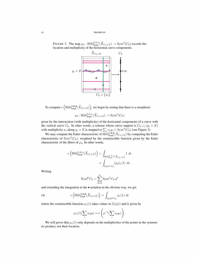
FIGURE 3. The map ρd : Hilb0,d,nfixed (XC0×E) → Symd(C0) records the

location and multiplicity of the horizontal curve components.

XC0×E C0

yi × E aiyi

C0 × {x0}

To compute e(

Hilb0,•,•fixed (XC0×E)

), we begin by noting that there is a morphism

ρd : Hilb0,d,nfixed (XC0×E)→ Symd(C0)

given by the intersection (with multiplicity) of the horizontal components of a curve withthe vertical curve C0. In other words, a scheme whose curve support is C0 ∪i (yi × E)

with multiplicity ai along yi × E is mapped to∑i aiyi ∈ Symd(C0) (see Figure 3).

We may compute the Euler characteristic of Hilb0,•,•fixed (XC0×E) by computing the Euler

characteristic of Symd(C0), weighted by the constructible function given by the Eulercharacteristic of the fibers of ρd. In other words,

e(

Hilb0,d,nfixed (XC0×E)

)=

∫Hilb0,d,n

fixed (XC0×E)

1 de

=

∫Symd C0

(ρd)∗(1) de.

Writing

Sym• C0 =

∞∑d=0

Symd C0 qd

and extending the integration to the • notation in the obvious way, we get

(4) e(

Hilb0,•,•fixed (XC0×E)

)=

∫Sym• C0

ρ∗(1) de

where the constructible function ρ∗(1) takes values in Z((p)) and is given by

ρ∗(1)(∑i

aiyi) = e

(ρ−1(

∑i

aiyi)

).

We will prove that ρ∗(1) only depends on the multiplicities of the points in the symmet-ric product, not their location.


Proposition 5.1. There exists a universal series F (a) ∈ Z[[p]] such that the constructiblefunction ρ∗(1) is given by

ρ∗(1)(∑

aiyi

)=

p

(1− p)2∏i

F (ai).

Deferring the proof of the proposition for the moment, we apply the following lemmaregarding weighted Euler characteristics of symmetric products.

Lemma 5.2. Let T be a scheme and let Sym•(T ) =∑∞d=0 Symd(T ) qd. Suppose that

G is a constructible function on Symd(T ) of the form G(∑i aiyi) =

∏i g(ai) where by

convention g(0) = 1. Then∫Sym• T

G de =

( ∞∑a=0

g(a) qa

)e(T )

.

This lemma is a consequence of the fact that symmetric products define a pre-lambdaring structure on the Grothendieck group of varieties and the Euler characteristic homo-morphism is compatible with that structure. An elementary proof is given in [4].

Applying Lemma 5.2 to Proposition 5.1 and combining with equations (2), (3), and (4)and we see that

(5) q DT0(X) =p

(1− p)2

( ∞∑a=0

F (a) qa

)2

·∞∏m=1

(1− qm)−22.

To finish the computation of DT0(X), we need to prove Proposition 5.1 and computethe series

∑a F (a)qa.

5.1. Proof of Proposition 5.1 and the computation of∑a F (a)qa. The fiber ρ−1(

∑aiyi)

parameterizes subschemes supported on XC0×E which have fixed curve support

C0 × x0 ∪i {yi} × Ewhere the multiplicity of the subscheme along {yi} × E is ai. Such a subscheme isuniquely determined8 by its restriction to the formal neighborhoods X{yi}×E and theircomplement U in XC0×E . The resulting stratification leads to a product decompositionfor the Grothendieck group valued power series ρ−1(

∑aiyi) giving the product formula

in Proposition 5.1. The factor p(1 − p)−2 comes from the contribution of U and it is theseries for the Hilbert scheme of subschemes of XC0×E with fixed curve support C0 × x0(no curves in the E direction). The moduli for this Hilbert scheme comes from floatingpoints and embedded points (see [4] for details).

The series F (a) is given by

F (a) = (1− p) · e(

Hilb0,a,•(X{yi}×E

))where


)⊂ Hilb0,a,•(X)

is the locus parameterizing subschemes Z whose curve support is given by the union ofC0 × {x0} and an a-fold thickening of {yi} × E and such that all embedded points of

8This follows from fpqc descent since the set U and the sets X{yi}×E form a fpqc cover. Since C0 × x0 isreduced there are no conditions on the overlaps of the cover. Thus the subscheme is uniquely determined by itsrestriction to the cover.

12 JIM BRYAN

Z are supported on X{yi}×E . The prefactor (1 − p) comes from the contribution of thecomplement U : the overall contribution of U is given by p(1 − p)−2+l where l is thenumber of yi’s and so we have redistributed the l copies of (1− p) into the F (ai) factors.

SinceX{yi}×E

∼= Spec (C[[u, v]])× E,we get an action of (C∗)2 on the corresponding Hilbert scheme. Only the (C∗)2 fixedpoints contribute to the Euler characteristic so

F (a) = (1− p) · e(


)(C∗)2)= (1− p)

∑α`a

e(

Hilb0,α,•(X{yi}×E

))where Hilb0,α,•

(X{yi}×E

)parameterizes subschemes whose curve component is the

unique curve given by the union of C0 × {x0} and Zα × E where Zα ⊂ Spec(C[[u, v]])is the length a subscheme given by the monomial ideal determined9 by the partition α ` a.

To compute e(

Hilb0,α,•(X{yi}×E

))we can now integrate over the fibers of the con-

structible morphismσ : Hilb0,α,•

(X{yi}×E

)→ Sym•E

which is defined by recording the length and locations of the embedded points. We thusget ∫

Hilb0,α,•(X{yi}×E)de =

∫Sym• E

σ∗(1) de.

The constructible function σ∗(1) is a product of local contributions which only depend onthe length of the embedded point and whether or not the location of the embedded pointis x0 or not (recall that x0 is where the curve C0 × {x0} is attached to the curve Zα × E). Writing the series for the local contributions at x0 and at the general point as V∅(1)α(p)and V∅∅α(p) respectively, and applying Lemma 5.2 we get∫

Sym• E

σ∗(1) de =(V∅(1)α(p)

)· (V∅∅α(p))

e(E−x0)

=V∅(1)α(p)

V∅∅α(p).

The above naming of the local contributions is not accidental — the generating func-tions for the contributions are given by the topological vertex. In general, the topologicalvertex Vµ1µ2µ3(p) can be defined as the generating function of the Euler characteristics

of the Hilbert schemes Hilbn(C3

0, {µ1, µ2, µ3})

, which by definition parameterize sub-

schemes of C3 given by adding at the origin a length n embedded point to the fixed curveZµ1∪ Zµ2

∪ Zµ3. Here Zµi is supported on the ith coordinate axis and given by the

monomial ideal determined by the partition µi in the transverse directions. Because (C∗)3

acts on these Hilbert schemes, their Euler characteristics can be computed by counting(C∗)3 fixed points, namely monomial ideals. This leads to the combinatorial interpreta-tion of Vµ1µ2µ3

(p) — it is the generating function for the number of 3D partitions withasymptotic legs given by {µ1, µ2, µ3}.

9i.e. identifying the partition α with its Ferrer’s diagram α ⊂ (Z≥0)2, the ideal of Zα is generated by the

monomials uivj where (i, j) 6∈ α.


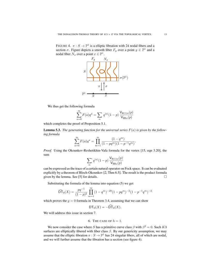
FIGURE 4. π : S → P1 is a elliptic fibration with 24 nodal fibers and asection σ. Figure depicts a smooth fiber Fy over a point y ∈ P1 and anodal fiber Nx over a point x ∈ P1.

Fy

y

Nx

x

σ(P1)

π σ

P1

S

We thus get the following formula∞∑a=0

F (a)qa =∑α

q|α|(1− p)V∅(1)α(p)

V∅∅α(p)

which completes the proof of Proposition 5.1.

Lemma 5.3. The generating function for the universal series F (a) is given by the follow-ing formula

∞∑a=0

F (a)qa =

∞∏m=1

(1− qm)

(1− pqm)(1− p−1qm).

Proof. Using the Okounkov-Reshetikhin-Vafa formula for the vertex [15, eqn 3.20], thesum ∑

α

q|α|(1− p)V∅(1)α(p)

V∅∅α(p)

can be expressed as the trace of a certain natural operator on Fock space. It can be evaluatedexplicitly by a theorem of Bloch-Okounkov [2, Thm 6.5]. The result is the product formulagiven by the lemma. See [5] for details. �

Substituting the formula of the lemma into equation (5) we get

DT0(X) =pq−1

(1− p)2∞∏m=1

(1− qm)−20(1− pqm)−2(1− p−1qm)−2

which proves the g = 0 formula in Theorem 3.4, assuming that we can show

DT0(X) = −DT0(X).

We will address this issue in section 7.

6. THE CASE OF h = 1.

We now consider the case where S has a primitive curve class β with β2 = 0. Such K3surfaces are elliptically fibered with fiber class β. By our genericity assumption, we mayassume that the elliptic fibration π : S → P1 has 24 singular fibers, all of which are nodal,and we will further assume that the fibration has a section (see figure 4).

14 JIM BRYAN

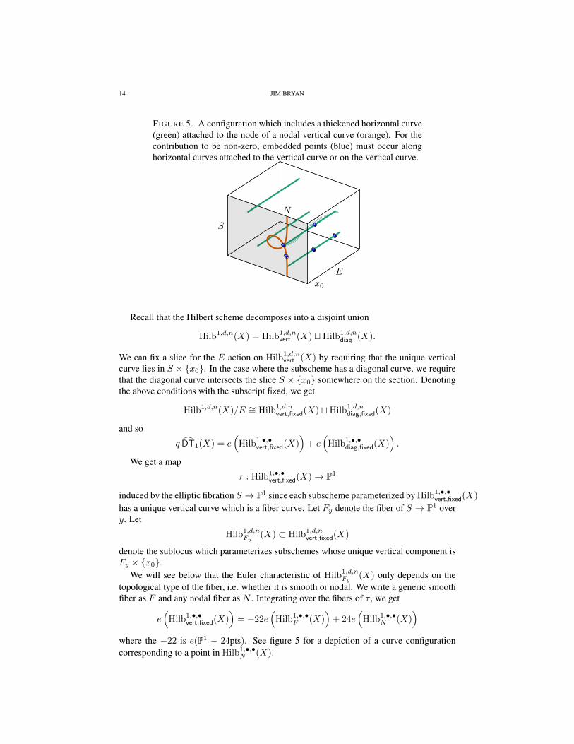
FIGURE 5. A configuration which includes a thickened horizontal curve(green) attached to the node of a nodal vertical curve (orange). For thecontribution to be non-zero, embedded points (blue) must occur alonghorizontal curves attached to the vertical curve or on the vertical curve.

N

S

E

x0

Recall that the Hilbert scheme decomposes into a disjoint union

Hilb1,d,n(X) = Hilb1,d,nvert (X) tHilb1,d,n

diag (X).

We can fix a slice for the E action on Hilb1,d,nvert (X) by requiring that the unique vertical

curve lies in S × {x0}. In the case where the subscheme has a diagonal curve, we requirethat the diagonal curve intersects the slice S × {x0} somewhere on the section. Denotingthe above conditions with the subscript fixed, we get

Hilb1,d,n(X)/E ∼= Hilb1,d,nvert,fixed(X) tHilb1,d,n

diag,fixed(X)

and so

q DT1(X) = e(

Hilb1,•,•vert,fixed(X)

)+ e

(Hilb1,•,•

diag,fixed(X)).

We get a map

τ : Hilb1,•,•vert,fixed(X)→ P1

induced by the elliptic fibration S → P1 since each subscheme parameterized by Hilb1,•,•vert,fixed(X)

has a unique vertical curve which is a fiber curve. Let Fy denote the fiber of S → P1 overy. Let

Hilb1,d,nFy

(X) ⊂ Hilb1,d,nvert,fixed(X)

denote the sublocus which parameterizes subschemes whose unique vertical component isFy × {x0}.

We will see below that the Euler characteristic of Hilb1,d,nFy

(X) only depends on thetopological type of the fiber, i.e. whether it is smooth or nodal. We write a generic smoothfiber as F and any nodal fiber as N . Integrating over the fibers of τ , we get

e(


)= −22e

(Hilb1,•,•

F (X))

+ 24e(

Hilb1,•,•N (X)

)where the −22 is e(P1 − 24pts). See figure 5 for a depiction of a curve configurationcorresponding to a point in Hilb1,•,•

N (X).


The computation of e(

Hilb1,•,•F (X)

)and e

(Hilb1,•,•

N (X))

follows the same strategy

as the computation of e(

Hilb0,•,•fixed (X)

)done in section 5. We use the product decompo-

sitions

Hilb1,•,•F (X) = Hilb1,•,•

F

(XF×E

)·Hilb1,•,• (X − F × E)(6)

Hilb1,•,•N (X) = Hilb1,•,•

N

(XN×E

)·Hilb1,•,• (X −N × E)(7)

and we use the extra E actions on the second factors to deduce

e(

Hilb1,•,•F (X)

)= e

(Hilb1,•,•

F

(XF×E

))·∞∏m=1

(1− qm)−24

e(

Hilb1,•,•N (X)

)= e

(Hilb1,•,•

N

(XN×E

))·∞∏m=1

(1− qm)−23

where 24 = e(S − F ) and 23 = e(S −N).Proceeding as we did in section 5, we use the maps

ρ : Hilb1,•,•F

(XF×E

)→ Sym•(F )

ρ : Hilb1,•,•N

(XN×E

)→ Sym•(N)

which record the location and multiplicity of the horizontal components. The argumentproceeds exactly as it did in section 5 with F and N playing the role of C0.

The result for the smooth fiber case is the following:∫Hilb1,•,•

F (XF×E)de =

∫Sym•(F )

ρ∗(1) de

=(p1/2(1− p)−1

)e(F )

·

( ∞∑a=0

F (a)qa

)e(F )

(8)

= 1.

This result comports with the heuristic thatF acts on XF×E and hence on Hilb1,•,•F

(XF×E

)and so the Euler characteristic is 0 except for the unique F -fixed subscheme, i.e. the sub-scheme consisting of just the curve F × {x0} with no added horizontal components orembedded points. However, this is only a heuristic: F does not act algebraically on theformal neighborhood XF×E since the elliptic fibration is not isotrivial10.

The situation for nodal fibers is a little different because of the presence of the nodalpoint z ∈ N . The constructible function ρ∗(1), which is given by taking the Euler charac-teristic of the fibers of the map

ρ : Hilb1,•,•N

(XN×E

)→ Sym•N,

has the following form. Let y1, . . . , yl be non-singular points of N and let z ∈ N bethe nodal point. Then ρ−1(bz +

∑aiyi) parameterizes subschemes of X , supported on

XN×E , which have fixed curve support

N × {x0} ∪ {z} × E ∪i {yi} × E

10However, see section 7 for the action of a related group.

16 JIM BRYAN

where the multiplicity along {z} × E is b and the multiplicity along {yi} × E is ai.Such a subscheme is determined by its restriction to the formal neighborhoods X{z}×E ,X{y1}×E , . . . , X{yl}×E and their complement U . The contribution of the Euler character-istic of U is given by

(1− p)−e(N◦) = (1− p)l

where N◦ = N − {z, y1, . . . , yl}. Therefore we see that

ρ∗(1)(bz +∑

aiyi) = N(b)

l∏i=1

F (ai)

where F (a) is as in section 5, and

N(b) = e(

Hilb1,b,•(X{z}×E

))where

Hilb1,b,n(X{z}×E

)⊂ Hilb1,b,n(X)

is the sublocus parameterizing subschemes Z whose curve support is given by the unionof N × {x0} and a b-fold thickening of {z} × E and such that all embedded points aresupported on X{z}×E .

So pushing the integral to Sym•N and applying lemma 5.2 we get∫Hilb1,•,•

N (XN×E)1 de =

∫Sym•N

ρ∗(1)de

=

∫Sym•(N−{z})

∏i

F (ai) de ·∫Sym•({z})

N(b) de

=

( ∞∑a=0

F (a)qa

)e(N−{z})·

( ∞∑b=0

N(b)qb

).

Note that e(N − {z}) = 0 so that the F (a) term doesn’t contribute.We compute the N(b) contribution by using the (C∗)2 action on

X{z}×E ∼= Spec(C[[u, v]])× E

and arguing as in section 5. We find∞∑b=0

N(b)qb =

∞∑b=0

e(

Hilb1,b,•(X{z}×E

))qb

=

∞∑b=0

∑β`b

e(

Hilb1,β,•(X{z}×E

))qb

=∑β

q|β|V(1)(1)β(p)

V∅∅β(p).

We see that fact that the curve N has a node is manifest in the term in the numerator:the vertex V(1)(1)β(p) is counting curve configurations which are locally monomial at thenodal point {z} × {x0} where the curve is degree 1 along the two branches of the nodeand has the monomial thickening given by β along the E direction.


Putting this and the earlier computations together, we find that the total contribution ofthe components with vertical curves is given by the following:

e(


)=− 22

∞∏m=1

(1− qm)−24 + 24

∞∏m=1

(1− qm)−23 ·∑β

q|β|V(1)(1)β(p)

V∅,∅,β(p)

= 24

∞∏m=1

(1− qm)−24

1

12− 1 +

∞∏m=1

(1− qm)∑β

q|β|V(1)(1)β(p)

V∅,∅,β(p)

.

Proposition 6.1. The following identity holds:∞∏m=1

(1− qm)∑β

q|β|V(1)(1)β(p)

V∅∅β(p)= 1 +

p

(1− p)2+

∞∑d=1

∑k|d

k(pk + p−k)qd.

Proof sketch: Using the Okounkov-Reshetikhin-Vafa formula for the topological vertex[15, Eqn 3.20], and some standard combinatorics, one can rewrite the left hand side ofthe above equation so that it is given in terms of Bloch-Okounkov’s 2-point correlationfunction [2, Eqn 5.2]. Namely, one can show that it is given by 1 − F (t1, t2) in the limitwhere t1 and t2 approach p and p−1 respectively. The limit can be evaluated explicitlyusing [2, Thm 6.1] and this leads to the right hand side of the formula. Details can befound in [5].

Plugging in the proposition’s formula into the previously obtained equation, we see thatthe non-diagonal contribution to DT1(X) is given as

e(


)= 24

∞∏m=1

(1−qm)−24

1

12+

p

(1− p)2+

∞∑d=1

∑k|d

k(pk + p−k)qd

6.1. Diagonal contributions. To finish our computation of DT1(X), it remains to com-pute e

(Hilb1,•,•

diag,fixed(X))

.Let C ⊂ X be a diagonal curve. The projections onto the factors of X = S×E induce

maps

pS :C → Fy

pE :C → E

where Fy is a fiber curve, and the maps have degree 1 and some d > 0 respectively. Fycannot be a nodal fiber since then C would have geometric genus 0 and consequently itwould not admit a non-constant map to E. The above maps induce a map

f : Fy → E

which must be unramified by the Riemann-Hurwitz formula. Thus the diagonal curve Cis contained in the surface Fy × E and is given by the graph of the map f . Recall that wefixed a slice for the E action on Hilb1,d,n

diag (X) by requiring that the diagonal curve meetsSx0

at the section; this is equivalent to requiring that f(s) = x0 where s ∈ Fy is thesection point on Fy . Up to automorphisms, such a map f must be a group homomorphismof the corresponding elliptic curves. Assuming that E is generic, so that the only non-trivial automorphism is given by x 7→ −x, we see that every diagonal curve (with the fixedcondition) is of the form

{(z, f(z)) ∈ Fy × E} or {(z,−f(z)) ∈ Fy × E}

18 JIM BRYAN

where f : Fy → E is a group homomorphism.The number of group homomorphisms of degree d to a fixed elliptic curveE is given by∑k|d k. This classical fact can be seen by counting index d sublattices of Z⊕ Z. For each

such cover, F → E, the domain elliptic curve will occur exactly 24 times in the fibrationS → P1. So we find that the total number of diagonal curves having degree d in the Edirection is

2 · 24∑k|d

k.

Each such diagonal curve can be accompanied by horizontal curves (with thickenings) aswell as embedded points. The contribution of these components of the Hilbert scheme iscomputed in exactly the same way as the contribution of the curves with a smooth verticalcomponent F . Recall that e

(Hilb1,•,•

F (X))

=∏∞m=1(1 − qm)−24. Taking into account

the degree of the diagonal curves, we thus find

e(

Hilb1,•,•diag,fixed(X)

)=

∞∏m=1

(1− qm)−24

2 · 24 ·∞∑d=1

∑k|d

kqk

.

Finally, adding the vertical and diagonal contributions together we arrive at

DT1(X) = 24q−1∞∏m=1

(1− qm)−24

1

12+

p

(1− p)2+

∞∑d=1

∑k|d

k(pk + p−k + 2)qd

.

Note that this formula is off from the desired formula for DTh=1(X) by an overall mi-nus sign and a minus sign on the 2. In fact we will see in section 7 that due to the Behrendfunction, the contribution of the diagonal components carry the opposite sign of the con-tribution of the vertical components. Denoting the contribution to DT1(X) coming fromHilb1,•,•

vert,fixed(X) and from Hilb1,•,•diag,fixed(X) by DT1,vert(X) and DT1,diag(X) respectively,

we find that we need to show

DT1(X) = −DT1,vert(X) + DT1,diag(X).

7. PUTTING IN THE BEHREND FUNCTION

The goal of this section is to prove, assuming Conjecture 7.1, the relations

DT0(X) = −DT0(X)

DT1(X) = −DT1,vert(X) + DT1,diag(X)

which is all that is needed to complete the proof of Theorem 3.4.

7.1. Overview. Our general strategy for computing DT(X), the unweighted Euler char-acteristics of the Hilbert schemes, utilized the following general scheme.

(1) Using the geometric support of curves (and/or points) of the subschemes, we strat-ified Hilb(X) such that the strata could be written as products of simpler Hilbertschemes.

(2) We utilized actions of C∗ or E which could be defined on individual factors in thestratification to discard strata not fixed by the action and restrict to fixed points.

(3) We found that some strata were parameterized by symmetric products, and wepushed forward the Euler characteristic computation to the symmetric productswhere we used Lemma 5.2.


(4) After possibly iterating steps (1)–(3), we reduced the computation to countingdiscrete subscheme configurations, namely those which are given formally locallyby monomial ideas. These we counted with the topological vertex.

In order to incorporate the weighting by ν, the Behrend function, into the Euler charac-teristics in the above strategy, we need to modify steps (2) and (4).

For (2) to apply to ν-weighted Euler characteristics, we need to know that ν, restrictedto the relevant stratum S ⊂ Hilb(X), is invariant under the action of the group. We can dothis by showing that the group (or possibly a modification of the group) acts on the formalneighborhood of S inside of Hilb(X). This works since the value of the Behrend functionat a point only depends on the formal neighborhood of the point.

To modify step (4), the final step, we will need to know the value of the Behrend functionat subschemes given formally locally by monomial ideals. In particular, we want to showthe value is given by ±1, where the sign alternates as n increases. This will account forthe relatively simple relationship between DT(X) and DT(X).

We are only partially able to succeed with the above modification. In the first twoiterations of steps (1), (2), and (3) of the strategy, we succeed in extending the actions ofthe group (or related group) to the formal neighborhood of the strata. However, in the finaliteration of (1)-(3), the (C∗)3 action we used on the strata does not obviously extend totheir formal neighborhoods (quite possibly such an extension does not exist). To remedythis situation, we must assume a conjecture first formulated in [4, Conj 18].

7.2. Elaboration. Let us expand on the above discussion to highlight the issues.In the first two iterations of steps (1), (2), and (3), we stratified by the curve support of

the subschemes. These strata decompose into the product given by the equations (1), (6),and (7) where the second factors correspond to connected components of the curve withpure vertical support. This factor admits an extra E action, and we wish to show that thisaction extends to the formal neighborhoods of the strata.

The formal neighborhood of a closed point in Hilb(X) parameterizes infinitesimal de-formations of the subscheme corresponding to the closed point. Connected components ofa subscheme deform independently from each other and consequently the products givenin equations (1), (6), and (7) extend to their formal neighborhoods, as do the E actions.

The first factor in the products (1), (6), and (7) correspond to subschemes supported inXC×E where C is the curve in the slice S × x0, which is either C0 (for h = 0), or N or F(for h = 1). This stratum was further stratified by the location of the vertical componentsof such curves. Each of these strata admits a C∗ × C∗ induced by the action

X{y}×E ∼= SpecC[[x, y]]× E,the formal neighborhood of a vertical component. This action does not obviously extendto the formal neighborhood of the strata in the Hilbert scheme. The basic issue is thefollowing.

A subscheme in X whose reduced support is

C × x0 ∪ y × Eand whose multiplicies along C × x0 and y ×E is 1 and some a ≥ 1 on E respectively isuniquely determined by its restrictions to

Xy×E and XC×X0− {y × x0}.

The action of C∗ × C∗ on Xy×E thus induces an action on this strata. However, it isnot clear if the action on this stratum extends to an action on its formal neighborhood due

20 JIM BRYAN

to (for example) the possibility of obstructed infinitesimal deformations of the subschemesmoothing the node.

We can circumvent this problem by using somewhat different group actions. In the caseof h = 0, the C∗ × C∗ action on Xy×E does extend to an action on XC0×E . The reasonis that C0 is a smooth −2 curve in a surface and consequently its formal neighborhoodin the surface is isomorphic to the formal neighborhood of the zero section in the totalspace of T ∗P1. This formal scheme carries an C∗ × C∗ action which can be choosen tobe compatible with the one on Xy×E . This then induces an action on Hilb(XC0×E)/Ewhich naturally extends to its formal neighborhood in Hilb(X)/E.

In the case of h = 1, we can also construct global group actions on XC×E , but differentfrom the C∗ × C∗ action previously used. For C = F , a smooth elliptic curve, we pre-viously noted that the action of F on F × E given by translation on the first factor, doesnot extend to XF×E . The reason is that the linear system of F in S induces a non-trivialelliptic fibration S → P1 and thus a non-trivial fibration SF → SpecC[[t]]. However,after choosing a section of the above map, SF is a group scheme over SpecC[[t]] and theMordell-Weil group of sections acts (freely) on SF , and thus on XF×E = SF × E. Thisinduces an action of the Mordell-Weil group on Hilb(XF×E)/E which extends to its for-mal neighborhood and is free whenever the degree in the vertical direction is non-zero. TheMordell-Weil group is an an extension of the group F by an additive group and so its orbitshave Euler characteristic zero. Consequently the conclusion expressed by equation (8) forthe usual Euler characteristics also applies to the ν-weighted Euler characteristics.

Similarly, the Mordell-Weil group of sections of SN → SpecC[[t]] acts on Hilb(XN×E)/Eand its formal neighborhood. This group is an extension of C∗ (the group of the nodalfiber) by an additive group and hence necessarily splits. Thus we get an action of C∗ onHilb(XN×E)/E which is compatible with the Behrend function. The fixed points are sub-schemes whose vertical part has support in X{z}×E where z ∈ N is the node. Moreover,the C∗ action here is given by λ(x, y) = (λx, λ−1y) for a suitable choice of isomor-phism X{z}×E ∼= E × SpecC[[x, y]]. The fixed subschemes under this action correspondto subschemes whose maximal Cohen-Macaulay subscheme is formally locally given bymonomial ideals.

Via the above, we have shown that the ν-weighted Euler characteristics of the Hilbertschemes are equal to the ν-weighted Euler characteristics of the locus in the Hilbert schemeparameterizing subschemes whose maximal Cohen-Macaulay subscheme is given formallylocally by monomial ideals.

In the final iteration of steps (1)-(3), we were able to further reduce to subschemeswhose embedded points are also local monomial. To achieve this we further stratifiedour strata by the location of the embedded points. We then used the action of (C∗)3 onthe formal neighborhoods of the embedded points to construct a (C∗)3 action on thesesubstrata. Unfortunately, we are unable to show that this action on the substrata extends toa formal neighborhood of the substrata. Consequently, we cannot show that the Behrendfunction is compatible with the action.

To circumvent this problem, we will assume the validity of the following conjecture,restated from [4, Conj 18]. Let Y be any quasi-projective Calabi-Yau threefold. LetC ⊂ Ybe a (not necessarily reduced) Cohen-Macaulay curve with proper support. Assume that


the singularities of Cred are locally toric11. Let

Hilbn(Y,C) = {Z ⊂ Y such that C ⊂ Z and IC/IZ has finite length n}.Note that Hilbn(Y,C) ⊂ Hilb(Y ) and let ν denote the Behrend function on Hilb(Y ).

Conjecture 7.1 ([4]).∫Hilbn(Y,C)

ν de = (−1)nν([C])

∫Hilbn(Y,C)

de,

where ν([C]) is the value of the Behrend function at the point [C] ∈ Hilb(Y ).

This conjecture allows us to promote the remaining part of our Euler characteristiccomputation to ν-weighted Euler characteristic, once we compute the value of the Behrendfunction at locally monomial Cohen-Macaulay subschemes. Suppose we could show thatvalue was always (−1)n where n is the holomorphic Euler characteristic of the subscheme,then, because of the (−p) built directly into the definition of DTg(X), we could concludethat DTg(X) = DTg(X) for h = 0 and h = 1. We will show this is nearly true: in fact theBehrend function has value −(−1)n for all curves in the h = 0 case and for those withoutdiagonal components in the h = 1 case. Curves with diagonal components have the sign(−1)n.

7.3. The Behrend function at Cohen-Macaulay subschemes. The only Cohen-Macaulaysubschemes which contribute to the invariants in our counting scheme are all of the fol-lowing form:

(1) Z × E,(2) C0 × x0 ∪ Z × E (h = 0),(3) N × x0 ∪ Z × E (h = 1), and(4) C, a diagonal curve (necessarily reduced)

where Z ⊂ S is a zero dimensional subscheme of length d. For each of these cases, weshow these subschemes lie in a smooth, open locus of the corresponding component of theHilbert scheme and hence the value of Behrend function is given by (−1)D where D is thedimension of that open set.

This is entirely parallel to the analysis in sections 8 and 9 of [4]. Namely, we constructan explicit D-dimensional family of such subschemes and we then show that the family issmooth by showing the Zariski tangent space also has dimension D.

Proposition 7.2. The following families of subschemes have the given dimensions and areopen sets of Hilbert scheme which are smooth at subschemes given locally by monomialideals.

(1) The locus of schemes of the form Z × E has dimension 2d, where Z ⊂ S is alength d zero-dimensional subscheme.

(2) The locus of schemes of the form C0 × x0 ∪ Z × E has dimension 2d− k, whereZ ⊂ S is a length d zero-dimensional subscheme such that length(C0 ∩ Z) = k.

(3) The locus of schemes of the form C×x0∪Z×E has dimension 2d−k+1, whereZ ⊂ S is a length d zero-dimensional subscheme such that length(C ∩ Z) = kand C ∈ |F | is any curve in the class F (including N ).

(4) The locus of diagonal curves has dimension 0.

11This means that formally locally Cred is either smooth, nodal, or the union of the three coordinate axes.That is at p ∈ Cred ⊂ Y the ideal ICred

⊂ OY,p is given by (x1, x2), (x1, x2x3), or (x1x2, x2x3, x1x3) forsome isomorphism OY,p ∼= C[[x1, x2, x3]].

22 JIM BRYAN

Proof. The family (1) is paramterized by Hilbd(S) which has dimension 2d. The family(2) is parameterized by the locus of points [Z] ∈ Hilbd(S) given by the codimensioncondition that length(Z ∩ C0) = k. This is smooth of dimension 2d− k by [4, Thm 20].The family (3) is parameterized by the locus of points [Z] ∈ Hilbd(S) such that length(Z∩C) = k for some C ∈ |F |. This family maps to |F | ∼= P1 with fibers of dimension 2d− k(again by [4, Thm 20]).

To complete the proof of the proposition, we want to show these sets are open andsmooth at the monomial ideals. It suffices to show that the dimension of the Zariski tan-gent space is of the given dimension. The tangent space of the Hilbert scheme at a givensubscheme Z is given by the group Hom(IZ ,OZ) ∼= Ext1(IZ , IZ). These Ext groupscan be computed at monomial ideals using the technique of [4, § 9]. Indeed, the proofof Thm 21 in [4] applies with minor modifications to the cases (1)-(3). Finally it is easyto see that a diagonal curve C ⊂ X is scheme-theoretically isolated up to translation byE. For example, since C is smooth and reduced, the Zariski tangent space is given byH0(C,NC/X). Here C is given as the graph of some homomorphism f : Fy → E andthus NC/X is given as the non-trivial extension of f∗NF/S ∼= OC by NC/Fy×E ∼= OC .Therefore H0(C,NC/X) ∼= C which corresponds to the translations by E. �

Using the normalization exact sequence, one easily computes n, the holomorphic Eulercharacteristic of the subschemes given by the four families in Proposition 7.2. Namely,

n =

0 for family (1)1− k for family (2)−k for family (3)0 for family (4)

Since the value of the Behrend function at a smooth point of dimension D is (−1)D, theabove formulas, along with Proposition 7.2 gives us

ν =

(−1)2d = 1 = (−1)n for family (1)(−1)2d−k = (−1)−k = −(−1)n for family (2)(−1)2d−k+1 = (−1)−k+1 = −(−1)n for family (3)(−1)0 = 1 = (−1)n for family (4)

In the h = 0 case, the locally monomial Cohen-Macaulay subschemes which contributeto the ν-weighted Euler characteristics are disjoint unions of curves in family (1) and asingle curve in family (2). Thus, they always come with the sign −(−1)n and we canconclude

DT0(X) = −DT0(X).

In the h = 1 case, the locally monomial Cohen-Macaulay subschemes without a diagonalcomponent which contribute to the ν-weighted Euler characteristics are disjoint unions ofcurves in family (1) with a single curve in family (3). Thus the contribution of the non-diagonal curves to DTh=1(X) is given by −DT1,vert(X).

Finally, locally monomial Cohen-Macaulay subschemes with a diagonal curve whichcontribute to the ν-weighted Euler characteristic are disjoint unions of curves in family(1) with a single curve in family (4). Thus the contribution of the diagonal curves toDTh=1(X) is given by DT1,diag(X).


Putting it all together we see that

DT0(X) = −DT0(X)

DT1(X) = −DT1,vert(X) + DT1,diag(X)

as desired which completes the proof of Theorem 3.4.

Acknowledgements. I’d like to thank George Oberdieck, Rahul Pandharipande, andYin Qizheng for invaluable discussions. I’ve also benefited with discussions with TomCoates, Sheldon Katz, Martijn Kool, Davesh Maulik, Tony Pantev, Balazs Szendroi, An-dras Szenes, and Richard Thomas. The computational technique employed in this paperwas developed in collaboration with Martijn Kool whom I owe a debt of gratitude. I wouldalso like to thank the Institute for Mathematical Research (FIM) at ETH for hosting myvisit to Zurich, and for Matematisk Institutt, UiO and Jan Christophersen for organizingthe 2017 Abel Symposium.

REFERENCES

[1] Kai Behrend. Donaldson-Thomas type invariants via microlocal geometry. Ann. of Math. (2), 170(3):1307–1338, 2009. arXiv:math/0507523.

[2] Spencer Bloch and Andrei Okounkov. The character of the infinite wedge representation. Adv. Math.,149(1):1–60, 2000. arXiv:alg-geom/9712009.

[3] Tom Bridgeland. Hall algebras and curve-counting invariants. J. Amer. Math. Soc., 24(4):969–998, 2011.arXiv:1002.4374.

[4] Jim Bryan and Martijn Kool. Donaldson-Thomas invariants of local elliptic surfaces via the topologicalvertex. arXiv:math/1608.07369.

[5] Jim Bryan, Martijn Kool, and Benjamin Young. Trace identities for the topological vertex. Selecta Mathe-matica, Jan 2017. arXiv:math/1603.05271.

[6] Robbert Dijkgraaf, Erik Verlinde, and Herman Verlinde. Counting dyons in N = 4 string theory. NuclearPhys. B, 484(3):543–561, 1997. arXiv:hep-th/9607026.

[7] Martin Eichler and Don Zagier. The theory of Jacobi forms, volume 55 of Progress in Mathematics.Birkhauser Boston, Inc., Boston, MA, 1985.

[8] Min-xin Huang, Sheldon Katz, and Albrecht Klemm. Elliptically fibered Calabi-Yau manifolds and the ringof Jacobi forms. Nuclear Phys. B, 898:681–692, 2015.

[9] Min-xin Huang, Sheldon Katz, and Albrecht Klemm. Topological string on elliptic CY 3-folds and the ringof Jacobi forms. J. High Energy Phys., (10):125, front matter+78, 2015. arXiv:math/1501.04891.

[10] D. Maulik, N. Nekrasov, A. Okounkov, and R. Pandharipande. Gromov-Witten theory and Donaldson-Thomas theory. I. Compos. Math., 142(5):1263–1285, 2006. arXiv:math.AG/0312059.

[11] G. Oberdieck and R. Pandharipande. Curve counting on K3 × E, the Igusa cusp form χ10, and de-scendent integration. In K3 surfaces and their moduli, volume 315 of Progr. Math., pages 245–278.Birkhauser/Springer, [Cham], 2016. arXiv:math/1411.1514.

[12] Georg Oberdieck. On reduced stable pair invariants. arXiv:math/1605.04631.[13] Georg Oberdieck and Aaron Pixton. Holomorphic anomaly equations and the Igusa cusp form conjecture.

arXiv:math/1706.10100.[14] Georg Oberdieck and Junliang Shen. Curve counting on elliptic Calabi-Yau threefolds via derived cate-

gories. arXiv:math/1608.07073.[15] Andrei Okounkov, Nikolai Reshetikhin, and Cumrun Vafa. Quantum Calabi-Yau and classical crystals. In

The unity of mathematics, volume 244 of Progr. Math., pages 597–618. Birkhauser Boston, Boston, MA,2006. arXiv:hep-th/0309208.

[16] Tony Pantev, Bertrand Toen, Michel Vaquie, and Gabriele Vezzosi. Shifted symplectic structures. Publ.Math. Inst. Hautes Etudes Sci., 117:271–328, 2013. arXiv:math/1111.3209.

[17] Yukinobu Toda. Stability conditions and curve counting invariants on Calabi-Yau 3-folds. Kyoto J. Math.,52(1):1–50, 2012. arXiv:math/1103.4229.

DEPARTMENT OF MATHEMATICS, UNIVERSITY OF BRITISH COLUMBIA, ROOM 121, 1984 MATHEMAT-ICS ROAD, VANCOUVER, B.C., CANADA V6T 1Z2

the donaldson-thomas theory of via the …jbryan/papers/k3xe.pdf · the donaldson-thomas theory of...

Documents