the dream framework: a logic-inspired approach to

The DReAM framework:a logic-inspired approach to

reconfigurable system modeling

PhD in Institutions, Markets and Technologies

Curriculum in Computer Science

XXX Cycle

By

Alessandro Maggi

2020

mailto:[email protected]

The dissertation of Alessandro Maggi is approved.

Program Coordinator: Rocco De Nicola, IMT School for Advanced Stud-ies Lucca

Supervisor: Prof. Rocco De Nicola, IMT School for Advanced StudiesLucca

Supervisor: Prof. Joseph Sifakis, Univ. Grenoble Alpes

The dissertation of Alessandro Maggi has been reviewed by:

Prof. Martin Wirsing, Ludwig-Maximilians-Universitat Munchen

Prof. Roberto Bruni, University of Pisa

In beloved memory of my grandmother,Annunziata Mastracca (June 3, 1921 - November 20, 2016)

Contents

Acknowledgements x

Vita and Publications xiii

Abstract xv

1 Introduction 11.1 Motivation . . . . . . . . . . . . . . . . . . . . . . . . . . . . 11.2 Problem statement . . . . . . . . . . . . . . . . . . . . . . . 31.3 Main contributions . . . . . . . . . . . . . . . . . . . . . . . 51.4 Outline . . . . . . . . . . . . . . . . . . . . . . . . . . . . . . 71.5 Origin of the material . . . . . . . . . . . . . . . . . . . . . . 8

2 Preliminaries 92.1 Approaches to software systems modeling . . . . . . . . . 10

2.1.1 Process Description Languages . . . . . . . . . . . . 112.1.2 Architecture Description Languages . . . . . . . . . 12

2.2 Approaches to components coordination . . . . . . . . . . 152.2.1 Exogenous coordination paradigms . . . . . . . . . 152.2.2 Endogenous coordination paradigms . . . . . . . . 16

2.3 BIP-based Formalisms . . . . . . . . . . . . . . . . . . . . . 172.3.1 BIP: Behavior, Interaction, Priority . . . . . . . . . . 172.3.2 Dynamic BIP . . . . . . . . . . . . . . . . . . . . . . 222.3.3 Dynamic Reconfigurable BIP . . . . . . . . . . . . . 25

vii

3 The L-DReAM framework 293.1 PIL-based systems . . . . . . . . . . . . . . . . . . . . . . . . 30

3.1.1 Propositional Interaction Logic (PIL) . . . . . . . . . 303.1.2 Interacting Components . . . . . . . . . . . . . . . . 313.1.3 Systems of components . . . . . . . . . . . . . . . . 323.1.4 Disjunctive and Conjunctive styles in PIL . . . . . . 34

3.2 L-DReAM Syntax and Semantics . . . . . . . . . . . . . . . 363.2.1 Static systems with PILOps . . . . . . . . . . . . . . 373.2.2 Disjunctive and Conjunctive styles in PILOps . . . 503.2.3 Parametric architectures and dynamic systems . . . 55

3.3 Encoding other formalisms . . . . . . . . . . . . . . . . . . 64

4 The DReAM framework 704.1 Structuring architectures . . . . . . . . . . . . . . . . . . . . 72

4.1.1 Component Types and component Instances . . . . 724.1.2 Motif modeling . . . . . . . . . . . . . . . . . . . . . 76

4.2 The DReAM coordination language . . . . . . . . . . . . . . 804.2.1 Declaration expansion for coordination terms . . . 814.2.2 Reconfiguration operations . . . . . . . . . . . . . . 834.2.3 Disjunctive and Conjunctive styles in DReAM . . . 884.2.4 Operational semantics . . . . . . . . . . . . . . . . . 91

4.3 Example systems . . . . . . . . . . . . . . . . . . . . . . . . 924.3.1 Coordinating flocks of interacting robots . . . . . . 924.3.2 Coordinating flocks of robots with stigmergy . . . . 954.3.3 Reconfigurable ring . . . . . . . . . . . . . . . . . . 964.3.4 Simple platooning protocol for automated highways 100

5 Executable implementation 1075.1 The jDReAM core architecture . . . . . . . . . . . . . . . . . 1085.2 The jDReAM extended architecture . . . . . . . . . . . . . . 1155.3 Use cases in practice . . . . . . . . . . . . . . . . . . . . . . 119

5.3.1 Coordinating flocks of robots . . . . . . . . . . . . . 1195.3.2 Reconfigurable ring . . . . . . . . . . . . . . . . . . 1225.3.3 Simple platooning protocol . . . . . . . . . . . . . . 124

viii

6 Concluding considerations 1296.1 Summing up . . . . . . . . . . . . . . . . . . . . . . . . . . . 1296.2 Related works . . . . . . . . . . . . . . . . . . . . . . . . . . 1326.3 Future work . . . . . . . . . . . . . . . . . . . . . . . . . . . 134

A Proofs 136A.1 Disjunctive to conjunctive transformation in PIL . . . . . . 136

B jDReAM code examples 139B.1 Coordinating flocks of interacting robots . . . . . . . . . . . 139B.2 Simple platooning protocol for automated highways . . . . 142

ix

Acknowledgements

The memory of the first time I walked through the walls ofLucca knowing I was there to stay is still vividly impressed inmy mind. It has been quite a long journey from that day, fullof twists and turns as any meaningful road in life truly worthtraveling along is. Seeing it through has been a challengingfeat, one that would have not been possible without the con-tribution and support of many people.

A major thank you goes to the SysMA research unit of IMT forhaving me and, more specifically, to its director Prof. RoccoDe Nicola, who introduced me to the field of formal meth-ods and process calculi guiding me through the PhD withpatience, kindness, and his signature constructive optimism.I owe him a lot both professionally and personally for his con-tinuous support and understanding.

Another major thank you goes to Prof. Joseph Sifakis, whoI must credit first and foremost for his inventive ideas thatsparked my interest and shaped all the work that led me tothis accomplishment. To him goes all my appreciation for hispassionate support, priceless insights, and frank exchangeswe had.

I am likewise grateful to the attention my external referees,Prof. Roberto Bruni and Prof. Martin Wirsing, have put intomy work, pushing me to keep improving it further.

Another thank you goes to Dr. Marinella Petrocchi and Prof.Francesco Tiezzi, who guided me in the first steps of the PhDwith a fruitful and stimulating collaboration which taught me

x

many important lessons on scientific research.

The most significant turning point in this path has undoubt-edly been my acceptance of a position at the Bank of Italyhalfway-through the PhD. Despite the challenge of continu-ing my research activity alongside the commitment of a full-time job, I managed to overcome it also thanks to the supportof many colleagues in the Bank.

In particular, I would like to thank the former head of theSupervision Inspectorate Dr. Carmelo Lattuca and the head ofthe On-site Inspection Planning Division Dr. Paolo Bernardinifor authorizing an extended leave from work which allowedme to finish my study period at the School.

I would also like to thank all the members of the Applied Re-search Team of the General Directorate for Information Tech-nology, where I currently work as a research staff member,and specifically the head of the unit Dr. Marco Benedetti andhis deputy Dr. Luigi Bellomarini for their understanding andopen support to my external research activities.

No journey is truly complete without travel companions. I amtruly grateful I had the opportunity to meet so many along theway, I want to take the time to thank the ones who are dearerto me one by one in no particular order.

Hanin, my dear coffee-pal, for all the coffees, the quality movieand TV-series recommendations, and especially the meaning-ful and inspirational conversations we had; Paolo, for sharingmany priceless moments, both fun and emotional, as well asone of the most peculiar cooking sessions involving a chickenand a can of beer; Luca, for all the funny moments and shower-related puns, as well as for being the best roommate one couldhope for; Valentina, for her ability of combining rock-solid de-termination with contagious glee, and for being the best part-

xi

ner in interdisciplinary projects and team-based card games;Valerio, for his self-irony, his infectious laughter, and his un-bounded passion for lemons; Vitaly, for his ever-so-slightlydecipherable poker-face and his big heart; Anita, for her en-thusiasm, kindness, and for being always there to help others;Claudia, for the shared immeasurable enthusiasm for tabletop-and video-games.

Most importantly, to all of them, thank you for your friend-ship and for the time we spent together.

Next, I wish to thank my closest friends, Francesco, Germanoand Valerio, who have always been there for me even whenwe were far apart and had less opportunities to hang out.

Many thanks to the brilliant “team members” Fabio and Saimir,always ready to pitch new ideas and arrange epic reunionsacross space and time ever since we met at the university.

Thank you also to the eclectic duo from my past life as juniorphysicist, Riccardo and Valerio, with whom I will always re-member some of the most peculiar moments of our life spentin a laboratory.

I also owe many thanks to my parents and my aunt Nuccia fortheir unconditional support and encouragement throughoutthese years.

Last, but definitely not least, I thank from the bottom of myheart my soulmate and wife Michela, who has always beenby my side encouraging me to do my best and to follow mydreams, giving me strength throughout this journey.

xii

Vita

March 22, 1985 Born, Rome, Italy

2008 Bachelor Degree in PhysicsFinal mark: 106/110Sapienza University of Rome, Rome, Italy

2008-2010 Collaborator journalistSoura Magazine, Unexplored Publishing LLC, Dubai,United Arab Emirates

2009-2015 Collaborator journalistNotebook Italia, Trani, Italy

2010 Bachelor Degree in Computer EngineeringFinal mark: 110/110Roma Tre, Rome, Italy

2013 Master Degree in Computer EngineeringFinal mark: 110/110 cum laudeSapienza University of Rome, Rome, Italy

2013-2015 PhotographerRPM Proget, Rome, Italy

2014 Business TechnologistCapgemini Italia, Rome, Italy

since 2014 PhD Candidate in Computer ScienceIMT School for Advanced Studies Lucca, Lucca, Italy

2016-2019 Administrative assistantSupervision Inspectorate, Bank of Italy, Rome, Italy

since 2019 ICT research staff memberApplied Research Team, Bank of Italy, Rome, Italy

xiii

Publications

1. R. De Nicola, A. Maggi, M. Petrocchi, A. Spognardi, and F. Tiezzi. “Twit-lang(er): Interactions Modeling Language (and Interpreter) for Twitter”.In: Proceedings of the 13th International Conference of Software Engineering andFormal Methods. Springer, 2015.

2. A. Maggi, M. Petrocchi, A. Spognardi, and F. Tiezzi. “A language-basedapproach to modelling and analysis of Twitter interactions”. In: Journal ofLogical and Algebraic Methods in Programming, vol. 87, 2017.

3. [43] R. De Nicola, A. Maggi, and J. Sifakis. “DReAM: dynamic reconfig-urable architecture modeling”. In: International Symposium on LeveragingApplications of Formal Methods. Springer, 2018.

4. [37] A. Maggi, R. De Nicola, and J. Sifakis. “A Logic-Inspired Approachto Reconfigurable System Modelling”. In: From Reactive Systems to Cyber-Physical Systems. Springer, 2019.

5. [18] R. De Nicola, A. Maggi, and J. Sifakis. “The DReAM framework fordynamic reconfigurable architecture modelling: theory and applications”.In: International Journal on Software Tools for Technology Transfer, 2020.

xiv

Abstract

Modern systems evolve in unpredictable environments andhave to continuously adapt their behavior to changing con-ditions. The DReAM (Dynamic Reconfigurable ArchitectureModeling) framework has been designed to address these re-quirements by offering the tools for modeling reconfigurabledynamic systems effectively.

At its core, the framework allows component-based architec-ture design leveraging a rule-based language, inspired fromInteraction Logic. The expressiveness of the language allowsus to define the behavior of both components and componentsaggregates encompassing all aspects of dynamicity, includingparametric multi-modal coordination of components and re-configuration of their structure and population.

DReAM allows the description of both endogenous/modu-lar and exogenous/centralized coordination styles and soundtransformations from one style to the other, while adopting afamiliar and intuitive syntax. To better model dynamic mobilesystems, the framework is further extended with two struc-turing concepts: motifs - independent dynamic architecturescoordinating components assigned to them - and maps - graph-like data structures modeling the topology of the environmentand parametrizing coordination between components.

The jDReAM Java project has been developed to provide anexecution engine with an associated library of classes andmethods that support system specifications conforming to theDReAM syntax. It allows to develop runnable systems com-bining the expressiveness of the rule-based notation with theflexibility of this widespread programming language

xv

Chapter 1

Introduction

1.1 Motivation

Depending on the perspective from which we examine a software sys-tem, we could consider it a procedure made of instructions that a machinecan understand and execute, a mathematical function that maps an in-put to an output, a circuit of elements in which data and control signalsflow through ports appropriately wired, and so on. Different aspects andproperties emerge by adopting one perspective or the other. The sameapplies if we shift our attention on the approaches to design such systems.Depending on the level of abstraction that we choose to adopt for eachelement that contributes to the definition of what a system does, we haveto account for a trade-off between expressive power, practical viability interms of actual instantiation and implementation, ease of human under-standing, and verifiability of desired properties (such as correctness andliveness).

Modern programming languages have reached a level of diffusionand maturity that arguably grants sufficient readability of code in addi-tion to high expressiveness and efficient execution. On the other hand,the challenges posed by the limits of verifiability of their broad capabili-ties and rich data types limits the kind of guarantees that we can obtain,so errors and unexpected behaviors are checked mostly during testing

1

and get patched even after the program is released. This is a standardpractice in the industry, and while there is no reason to require that everysingle line of code of every software has to be error-free from the day ofrelease, there are two exceptions that require additional guarantees:

1. critical systems whose correctness has direct implications for humanhealth and safety: potential faults have to be tracked and fixed be-fore they manifest during execution, as the consequences can bemajor and irreversible;

2. open systems executing in an unpredictable environment and coor-dinating with third-party agents not known a priori: correctnesschecks of system code could be not enough as unexpected, erro-neous behaviors can emerge from the interaction with external enti-ties.

The ever increasing complexity of modern software systems has changedthe perspective of software designers who now have to consider newclasses of them, consisting of a large number of interacting componentsand featuring complex interactions. These systems are usually distributed,heterogeneous, decentralized and interdependent, and are operating inan unpredictable environment. Such level of complexity calls for new ap-proaches to software design taking advantage of decomposition, indirec-tion and adaptation, as the lack of rigorous methodologies and formallygrounded modeling frameworks increases the risks of undesirable inter-ference and unpredictable outcomes. To cope with these issues, softwareneeds to be developed in such a way that systems can continuously adaptto internal changes and to changes in their operating environment.

The notion of “adaptation” directly ties in with that of “reconfigura-tion” capability, which allows to capture the dynamic aspects of modernsoftware already at design-time. Integrating these capabilities in the de-sign process is even more challenging for frameworks that aim at model-ing architectures, as they require to support both parametric systems in-stantiations and dynamic reconfigurations of their inner structure and oftheir coordination patterns. Software architectures are crucial in softwaredevelopment as they represent the fundamental structures upon which

2

individual systems are built. Effective architecture modeling supportsefficient and correct development by encouraging modularity, separationof concerns, and rationalization of recurring scenarios into “patterns” and“styles”. Despite the challenges, these benefits are all the more neededfor the classes of systems that we described. Architecture modeling lan-guages should be expressive enough to support these features while offer-ing an intuitive syntax and clear design methodologies in order to fostertheir practical use.

1.2 Problem statement

One of the main challenges that formalized approaches to complex sys-tems specification have to face is how to capture their dynamic aspectsand how to integrate them in a rigorous and controlled way in the designprocess. Dynamism, indeed, plays a crucial role in these modern systemsand can be guaranteed by exploiting the expressive power offered by thethree following features:

1. the parametric description of interactions between instances of com-ponents for a given system configuration;

2. the reconfiguration involving creation/deletion of components andmanagement of their interaction according to a given architecturalstyle;

3. the migration of components between predefined architectural styles.

The first feature implies the ability of describing the coordination ofsystems that are parametric with respect to the number of instances oftypes of components; examples of such systems are Producer-Consumersystems with m producers and n consumers or Ring systems consistingof n identical interconnected components.

The second feature is related to the ability of reconfiguring systemsby creating or deleting components and managing their interactions tak-ing into account the dynamically changing conditions. In the case of areconfigurable ring this would require having the possibility of removing

3

a component which self-detects a failure and of adding it back after recov-ery. Added components are subject to specific interaction rules accordingto their type and their position in the system. This is especially true formobile components which are subject to dynamic interaction rules de-pending on the state of their neighborhood.

The third aspect is related to the vision of “fluid architectures” [24]or “fluid software” [55]. The underlying idea is that applications and“smart” objects live in an environment which corresponds to an architec-tural style that defines how these entities behave and interact. Systems’dynamicity is modeled by allowing such entities to migrate among differ-ent environments; this dynamic migration allows a disciplined and easy-to-implement management of dynamically changing coordination rules.For instance, self-organizing systems may adopt different architecturalstyles to adapt their behavior in order to guarantee global properties.

The different approaches to architectural modeling and the new trendsand needs are reviewed in detailed surveys such as [13, 16, 38, 39, 45].Here, we consider two criteria for the classification of existing approaches:exogenous vs. endogenous and conjunctive vs. disjunctive modeling.

Exogenous modeling assumes that components are architecture-agnosticand guarantee a strict separation between a component behavior and itscoordination. Coordination is specified globally by rules applied to setsof components. The rules involve synchronization of events betweencomponents and associated data transfer. This approach is adopted byArchitecture Description Languages (ADL) [38]. It has the advantage ofproviding a global view of the coordination mechanisms and their prop-erties.

Endogenous modeling requires adding explicit coordination primitivesin the code describing components behavior. Components are composedthrough their interfaces, which are used to expose their coordination ca-pabilities. An advantage of endogenous coordination is that it does not re-quire programmers to explicitly build a global coordination model. How-ever, validating a coordination mechanism and studying its propertiesbecomes much harder without such a model.

Conjunctive modeling uses logic to express coordination constraints

4

between components. In particular, it allows modular description of com-pound systems as one can associate with each component its coordinationconstraints. The global coordination of a system can then be obtained asthe conjunction of individual constraints of its constituent components.

Disjunctive modeling consists in explicitly specifying system coordina-tion as the union of executable coordination mechanisms such as sema-phores, function call and connectors.

Merits and limitations of the two approaches are well understood.Conjunctive modeling allows abstraction and modular description butit is exposed to the risk of inconsistency in case there is no architecturesatisfying the specification. Conversely, disjunctive modeling by con-struction does not expose system designers to this risk, but requires thedefinition of monolithic connectors that usually have strong dependen-cies with other parts of the system and thus have limited reusability.

Many approaches for software architecture modeling have been pro-posed in literature with varying degrees of formalization, but to the bestof our knowledge none of them provides a generalized foundation ca-pable of capturing all the listed modeling criteria while also supportingdynamic reconfiguration and architectural style changes at runtime.

1.3 Main contributions

This thesis details two closely connected formal frameworks for the spec-ification of software architectures which natively support dynamism andadvanced reconfiguration capabilities. Both offer rigorous methodologiesfor architecture design by adopting a logic-based modeling language thatis expressive and powerful enough to support different approaches tocoordination and all the key features required to capture dynamicity. Assuch, the two frameworks do not impose limits to the coordination andcomputation styles, allowing instead to formalize sound transformationsbetween different design approaches.

L-DReAM - Light Dynamic Reconfigurable Architecture Modeling -is the most “unstructured” of the two frameworks aimed at capturing

5

all the core aspects of the underling modeling language with minimaloverhead.

In L-DReAM a system is a hierarchical structure of components. Eachnon-atomic component hosts a “pool” of components and defines thecoordination rules that regulate the way they interact and evolve. Theoverall structure of systems can also change as components can leaveand join different pools. Components will thus be subject to differentcoordination rules as they change their position in the hierarchy.

L-DReAM rules include an interaction constraint, modeled as a for-mula of the Propositional Interaction Logic (PIL) [11], and some opera-tions allowing data transfer as well as more complex reconfigurations ofthe component’s state. Parametric coordination between classes of com-ponents is achieved through the introduction of the concepts of componenttypes - blueprints for actual components - and component instances createdfrom specific types. Their coordination is characterized by rules in a firstorder extension to PIL with quantification over instance variables of agiven type.

DReAM - Dynamic Reconfigurable Architecture Modeling - can bethought as a specialization of L-DReAM to model systems that do not re-quire unbounded, free-form structures of components, but instead adoptsa hierarchy that adequately fits concrete systems and integrates additionalparametrization structures that make the design of dynamic and mobilearchitectures more intuitive and efficient.

In DReAM, a system consists of instances of types of components or-ganized in hierarchies of “motifs”. Component instances can migratebetween motifs depending on specific conditions. Thus, a given type ofcomponent can be subject to different rules when it is in a “ring” mo-tif or in a “pipeline” one. Motifs themselves are typed, and each motifinstance can migrate from one to another, dynamically changing theirhierarchy and thus potentially affecting all the underlying components.Using motifs allows a natural description of self-organizing systems.

Coordination rules in a motif are defined according to the same corelanguage used by L-DReAM. To enhance the expressiveness of the differ-

6

ent kinds of dynamism, each motif is also equipped with a “map”, whichis a graph defining the topology of the interactions in the motif. Compo-nents are associated with locations of the map via an addressing function@ which defines the position @(c) in the map of any component instancec associated with the motif. Additionally, each location is equipped witha local memory that can be accessed by components and used as a sharedmemory. Maps are also very useful to express mobility, in which casethe connectivity relation of the map represents possible moves of compo-nents. Finally, DReAM allows us to modify maps by adding or removinglocations and edges, as well as to dynamically create and delete compo-nent instances.

1.4 Outline

The rest of the thesis is organized as follows.Chapter 2 gives an overview of the “setting” in which the problem

of defining software intensive systems has been faced so far, focusingon how different approaches handle the architectural aspects of systemdefinitions, how they capture dynamic characteristics of the systems atruntime, and to what extent they support adaptation through reconfigu-ration of their structure and behavior. This chapter will also present someof the main formalisms that have inspired the development of the twoframeworks described in this thesis.

Chapter 3 introduces L-DReAM, a “light” variant of the DReAM frame-work that shares its approach on coordination of components but retainsa simpler syntax and a looser structure, making it very flexible and moresuitable to study fundamental properties of the underlying language. Thepresentation of the framework is done incrementally, starting from a sim-ple static setting where components interact according to formulas of thePropositional Interaction Logic (PIL), and proceeding upwards by firstadding data transfer between components and then reconfiguration ca-pabilities.

Chapter 4 presents the fully-structured DReAM framework detailingits key concepts and features, both in terms of their role in addressing the

7

requirements for dynamic and reconfigurable architecture modeling aswell as in the way they tie in with fundamental L-DReAM concepts. Tohighlight the distinguishing characteristics of DReAM with respect to itslight variant and other formalisms, we discuss few specific use cases thattake full advantage of the capabilities of the framework.

Chapter 5 describes the prototype Java-based modeling and executionframework jDReAM with a detailed overview of its architecture. The corecomponents of jDReAM implement the abstract syntax of L-DReAM andits operational semantics, while a dedicated library extends the API inorder to support DReAM specifications natively.

The concluding Chapter summarizes the main contributions and re-sults, briefly highlights similarities and differences between related worksand the presented frameworks, and discusses directions for future workboth from a theoretical and practical standpoint.

1.5 Origin of the material

The contents of this Thesis refer to and expand upon the following publi-cations:

[43] R. De Nicola, A. Maggi, and J. Sifakis. “DReAM: dynamic recon-figurable architecture modeling”. In: International Symposium onLeveraging Applications of Formal Methods. Springer, 2018.

[37] A. Maggi, R. De Nicola, and J. Sifakis. “A Logic-Inspired Approachto Reconfigurable System Modelling”. In: From Reactive Systems toCyber-Physical Systems. Springer, 2019.

[18] R. De Nicola, A. Maggi, and J. Sifakis. “The DReAM frameworkfor dynamic reconfigurable architecture modelling: theory and ap-plications”. In: International Journal on Software Tools for TechnologyTransfer, 2020.

8

Chapter 2

Preliminaries

Software systems have reached a level of complexity that calls for morerigorous approaches to software design. When applied to classes of sys-tems that globally consist of countless interacting components and featurecomplex interaction patterns, the lack of rigorous methodologies and for-mally grounded frameworks for modeling them increases the risks ofundesirable interference and unpredictable outcomes. These risks areamplified by the fact that these systems are usually distributed, heteroge-neous, interdependent, and are operating in unpredictable environments.To cope with these issues, software needs to be developed in order tocontinuously adapt to internal changes and to external ones happeningin the environment.

Correct design of such systems, even those traditionally not classifiedas “critical”, is becoming more and more important as they become in-creasingly interconnected and the fault of few can cause ripple effects onmany others. This challenge has been faced by practitioners using twovery distinct approaches:

1. a “production-centric” approach revolving mainly on organizationalframeworks for the software life-cycle management that leveragebest practices to guide software design and development;

2. a “formal” approach providing sound mathematical models of com-

9

putation that can be used to specify software systems and verifyqualitative and quantitative properties theoretically.

Discussing the merits and limitations of the former approach is beyondthe scope of this Thesis, which will focus on the latter instead.

This Chapter is organized as follows.Section 2.1 presents an overview of two different approaches to soft-

ware modeling, namely Process Description Languages and Architecture De-scription Languages.

Section 2.2 shifts the perspective to coordination paradigms forcomponent-based software modeling, comparing the exogenous coordina-tion approach with the endogenous one.

Section 2.3 focuses on the BIP framework and some of the main rep-resentatives of its derived formalisms showing how they relate with thetaxonomy discussed in Section 2.2. This will also provide the basis uponwhich the frameworks discussed in this Thesis have been devised.

2.1 Approaches to software systems modeling

To formalize a system specification there are many approaches that canbe adopted which depend on the perspective that we assume. We couldfocus on the description of how individual elements of a system behaveby defining precise rules that allow to reconstruct the exact executiontrajectory down to its sequence of states. However, if we are more inter-ested in capturing dependency relationships between components thatconstitute a system and how they interact with one another, we mightadopt instead an approach that highlights the overall structure of thesystem and treats other aspects with coarser approximation. These arejust two examples in a wide range of different dimensions in which it ispossible to organize the many formalisms and frameworks that allow towrite software-intensive system specifications. Among these, two broadcategories relating to the two orthogonal perspectives that we have justintroduced are Process Description Languages and Architecture DescriptionLanguages.

10

2.1.1 Process Description Languages

Process Description Languages (PDLs) are backed by a rich theory de-veloped in the last three decades that formalizes the semantics of concur-rent programming allowing to understand various functional and non-functional aspects of concurrent, distributed and mobile systems.

As of now there exist a large number of instances of PDLs, but over-all they share a common ground: they can be generally described asaction-based formalisms relying on behavioral operators that support com-positionality and abstraction, where the meaning of process terms is for-mally defined via structural operational semantics rules that induce astate transition graph over the process term.

Compositionality and abstraction are key concepts in the formalismas they enable the definition of behavioral equivalences. Such equivalencespermit manipulations at syntax and semantics level that allow to focuson specific aspects of a system and to fix the necessary granularity of thespecification by possibly abstracting from unnecessary details. By exploit-ing them it is possible to verify whether a system behavior conforms to agiven specification, i.e., a reference model describing the expected abstractbehavior of an application. This approach is generally called equivalencechecking.

PDLs, when equipped with an operational semantics, do support alsoanother kind of verification technique known as model checking. The goalof this approach is to verify whether a given system satisfies some proper-ties, often expressed via an appropriate logic. The fundamental differencebetween model checking and equivalence checking lies in the fact thatproperties need not be a full specification of the intended behavior, butthey might deal with specific characteristics of the system (e.g. deadlockfreedom).

Notable representatives of PDLs well recognized in scientific literatureare, among others, CSP (Communicating Sequential Processes) [28, 29],CCS (Calculus of Communicating Systems) [40] and π-calculus [41].

The expressive power and flexibility of this class of formalisms lentthemselves to extensions that go beyond the initial scope of modeling

11

functional system behavior. Few examples of them allowing to capturequantitative features are timed and probabilistic process calculi [3, 26, 44].

2.1.2 Architecture Description Languages

Architecture description languages (ADLs) are formal languages that can beused to represent the architecture of a software-intensive system. Withthe term architecture we refer to the description of the components thatcomprise a system, the behavioral specifications of those components,and the patterns and mechanisms for their interactions. Note that a sin-gle system is usually composed of more than one type of component:modules, tasks, functions, etc. An architecture can choose the type ofcomponents most appropriate or informative, or it can include multipleviews of the same system, each illustrating different components.

As software architectures became a dominating theme in large systemdevelopment and acquisition, methods for unambiguously specifyingthem have become more and more important. The main notions werealready identified in the early ’90s [25, 57]: components abstracting com-putations and data repositories, connectors abstracting the interactionprotocols used among components. Since then, a rich research literaturehas accompanied the development of several ADLs, experimenting withdifferent approaches to architecture specification.

Despite the efforts put into place by the scientific community, rigor-ous approaches to software architectures have yet to reach mainstreamattention within the community of developers. Indeed, as highlighted in[38] and [58], the process of software development in the industry hasbeen heavily influenced by organizational frameworks fostering “agile”methodologies that encourage quick iterations and fast prototyping, buthas not yet tied these practices with formalized frameworks that bind ar-chitectural descriptions with their implementations. In fact, practitionersare still heavily relying on informal circle-and-line drawings and semi-formal approaches that exhibit very weak support for architecture speci-fication such as UML [32]. This makes traceability between architecturaldocumentation and actual code ambiguous and challenging, diminish-

12

ing the incentive to keep the former up-to-date with the latter, which inturn discourages a wider adoption of structured approaches addressingarchitectural aspects of software design like ADLs.

However, agile development is not inherently in contrast with rigor-ous architecture description approaches. The reasons behind the “resis-tance” to ADLs adoption are manifold. On one hand the constellation ofproposed languages and their different characteristics prevents potentialadopters to get a clear picture of what each one has to offer and how usingthem could be beneficial in the scope of software development. Further-more surveys on the main acknowledged ADLs [17, 22, 47] have revealedthe presence of “gaps” in the formal semantics associated to some of thelanguages, thus making early analysis of system architectures in such in-stances difficult or even impossible. Paired with what seems to be one ofthe biggest obstacles in the adoption - i.e. the complexity of the languagesand the absence of an industrial standard [38] - this results in spotty usageof the more sophisticated languages for architectures specification.

Commonalities and discriminators among ADLs

Early architecture description languages such as ArTek [56], CODE [42],COMMUNITY [21], Darwin [36], Demeter [48], Modechart [34], PSDL/-CAPS [8], Rapide [35], Resolve [19], UniCon [54] and Wright [4], providedan already rich and diversified collection of approaches to the problembefore the turn of the century.

Comparative studies [17] showed how each language agreed on anumber of common aspects that contributed to an empirical notion ofwhat constitutes an ADL, and conversely exhibited differentiating fac-tors that traced back to the area of expertise of the groups behind theirdevelopment.

Among the common characteristics shared by most of these ADLs itis worth mentioning:

– presence of a formally-defined graphical and textual syntax (usuallyaccompanied with the respective semantics);

13

– capability to handle data flow and control flow as interconnectionmechanisms;

– support for creation, validation and refinement of architectures;

– ability to represent hierarchical levels of detail and to handle multipleinstantiations of templates;

– absence of significant support for capturing design rationale and/orhistory.

Among the discriminant aspects which differentiated these earlyADLs the following stand out:

– ability to handle real-time constructs at the architectural level;

– support for specification of particular architectural styles;

– ability to allow a user to define new types of components and connectors,define new statements and represent non-architectural information;

– possibility of user-defined definitions of the concept of “consis-tency”;

– ability to handle variability at the level of architecture instantiation;

– support to systems analysis.

The last point of discrimination deserves additional attention becauseproviding means to perform analysis of architectures is in fact one of themain arguments supporting the usage of ADLs against general-purposelanguages like UML.

Indeed while most of the languages supported analysis capabilities,in their initial versions few of them provided actual tools to perform ar-chitecture analysis. Among those which offered such tools, the approachto analysis was also very different between one another. For instance,Rapide features a discrete-event simulator based on partially-orderedsets of event behaviors, while Modechart uses a model-checker to verify

14

whether a system description guarantees, prohibits or is compatible witha given logical assertion.

More recent languages for architecture design - such as AADL [20],ADR [15], Alloy [33], CONNECT [31], COSA [46], PiLar [53], PRISMA[49] and SOFA [52] - proved to offer consistently a broader coverage offeatures while balancing out complexity by narrowing their scope (e.g.,enabling specification of architectural styles but limiting it to their coor-dination patterns, or offering complete typing of structural concepts andequivalence relations between them but only for static parametric sys-tems). As shown in [47], the diversification process involved mainly thefocus on specific capabilities of the language or the support tools, but theycan be roughly arranged in two broad categories: the component-only ap-proach and the component-and-connector one. We will go into more detailson them and how they compare to each other in section 2.2.

2.2 Approaches to components coordination

In section 2.1 we provided an overview of two broad categories of ap-proaches to model software-intensive systems. Another way of lookingat them is focusing on the way coordination between elements of such sys-tems is realized, i.e., how to define which actions synchronize/interleaveand under which circumstances. We can single out two main coordina-tion paradigms, namely the exogenous and the endogenous ones.

2.2.1 Exogenous coordination paradigms

The exogenous approach to coordination assumes that components arearchitecture-agnostic, self-contained building blocks that can be com-bined to form a complex system by “gluing” them together. The gluehere is what defines coordination between components, and can be spec-ified in multiple ways, e.g. by means of specific connectors that defineexplicitly which components can interact, under which conditions and towhat effect.

This paradigm guarantees a strict separation between a component

15

behavior and its coordination capabilities with other components. Assuch, it is conceptually closer to the domain of ADLs.

One of the main advantages of the exogenous approach is that com-ponents can be designed individually as they are architecture and coordi-nation agnostic, and thus support code reuse. The architecture defininghow components interact and communicate (i.e., the glue) can be de-signed separately, and to do so only some knowledge of the interface ofthe involved components (i.e., the minimal information that character-izes their endpoints for interaction) is required. An approach that can beconsidered a representative of this paradigm is REO [5], which indeedfocuses purely on the composition of connectors abstracting the innerbehavior of components.

This “global” perspective from which coordination between compo-nents is defined offers full expressive power to realize any interactionpattern, but for large systems it can make architecture specification cum-bersome as it cannot always be developed incrementally.

2.2.2 Endogenous coordination paradigms

The endogenous approach requires adding explicit coordination primitivesin the code describing components behavior.

Many PDLs can be related to this approach: for example all thosewhere synchronization between components happens by matching com-patible actions embedded in their individual behaviors (e.g., the interfaceparallel operator in CSP). Systems specified with this paradigm can bebuilt incrementally by composing individual components via specific op-erators such as the parallel composition and the interface parallel.

An advantage of endogenous coordination is that it does not requireprogrammers to explicitly build a global coordination model when writ-ing the specification of a system. The coordination model emerges asthe result of the composition of individual behaviors in which the com-munication actions are embedded. However, validating a coordinationmechanism and studying its properties becomes much harder withoutsuch a coordination model, requiring specific techniques (such as model

16

checking for process calculi) that usually can only be applied to subsetsof a system, simplified versions of it, or under specific hypotheses.

2.3 BIP-based Formalisms

BIP can be considered a “close relative” of ADLs in which systems aredefined as sets of components glued together using connectors. Despitesharing some structuring concepts and a fundamentally exogenous coor-dination approach, BIP differentiates from many ADLs in that it offersa fully formalized operational semantics, a mathematical model to rep-resent, combine and analyze interactions, and a comprehensive set oftools for code synthesis, embedding and verification. This makes BIP aviable choice to design and model different classes of systems, but alsoa robust platform upon which several modeling formalisms have beenbuilt - including the frameworks covered by this Thesis.

2.3.1 BIP: Behavior, Interaction, Priority

BIP was developed to model heterogeneous real-time component-basedsystems. Within the framework, components are obtained as the super-position of three layers that give name to the framework itself: Behavior,Interaction between transitions of the behavior in the form of a set of con-nectors, and Priority to describe the scheduling policies of interactions.

The framework is designed to allow incremental construction of sys-tems starting from atomic components (see figure 2) combined througha parametrized binary composition operator [27] that acts on each respec-tive layers separately and preserves deadlock-freedom. Parameters areused to define new interactions as well as new priority rules between thecomposed components.

BIP also supports heterogeneity by providing two mechanisms forstructuring interaction: rendezvous for strong synchronization, and broad-cast for weak synchronization.

17

Atomic components The structured syntax of atomic components isreported in figure 1. Atomic components in BIP are characterized by:

– a set of ports P = {p1 . . . pn}, names used for synchronization withother components;

– a set of control states S = {s1 . . . sk}, denoting locations at whichcomponents wait for synchronization;

– a set of variables V used to store data;

– a set of transitions modeling atomic computation steps, each onebeing a tuple of the form (s1, p, gp, fp, s2) representing a step fromcontrol state s1 to s2 with guard gp (Boolean condition on V ) andinternal computation fp on V .

It should be noted that guards and statements in the behavior of the com-ponent are C expressions and statements, respectively, and that they arerestricted with the assumption of atomicity for transitions (e.g. they haveno side-effects and their termination is guaranteed).

transition means that the associated guard is true and theinternal computation microstep is empty. The syntax foratomic components in BIP is the following:

atom::=component component id

port port id+

[data type id data id+]behavior{state state id

{on port id [provided guard][do statement] to state id}+}+

endend

That is, an atomic component consists of a declaration fol-lowed by the definition of its behavior. Declaration consistsof ports and data. Ports are identifiers and for data, basic Ctypes can be used. In the behavior, guard and statementare C expressions and statements respectively. We assumethat these are adequately restricted to respect the atomicityassumption for transitions e.g. no side effects, guaranteedtermination.

Behavior is defined by a set of transitions. The keywordstate is followed by a control state and the list of outgoingtransitions from this state. Each transition is labelled by aport identifier followed by its guard, function and a targetstate.

The BIP description of the reactive component of fig-ure 1 is:

component Reactiveport in, outdata int x, ybehavior

state emptyon in provided 0 < x do y:=f(x) to full

state fullon out to empty

endend

2.2. Connectors and Interactions

Components are built from a set of atomic componentswith disjoint sets of names for ports, control states, variablesand transitions.

Notation: We simplify the notation for sets of portsin the following manner. We write p1|p2|p3|p4 for theset {p1, p2, p3, p4} by considering that singletons are com-posed by using the associative and commutative operation|.

A connector γ is a set of ports of atomic componentswhich can be involved in an interaction. We assume that

connectors contain at most one port from each atomic com-ponent. An interaction of γ is any non empty subset of thisset. For example, if p1, p2, p3 are ports of distinct atomiccomponents, then the connector γ = p1|p2|p3 has seveninteractions: p1, p2, p3, p1|p2, p1|p3, p2|p3, p1|p2|p3. Eachnon trivial interaction i.e., interaction with more than oneport, represents a synchronization between transitions la-beled with its ports.

Following results in [11], we introduce a typing mech-anism to specify the feasible interactions of a connector γ,in particular to express the following two basic modes ofsynchronization:

• Strong synchronization or rendezvous, when the onlyfeasible interaction of γ is the maximal one, i.e., it con-tains all the ports of γ.

• Weak synchronization or broadcast, when feasible in-teractions are all those containing a particular portwhich initiates the broadcast. That is, if γ = p1|p2|p3

and the broadcast is initiated by p1, then the feasibleinteractions are p1, p1|p2, p1|p3, p1|p2|p3.

The typing mechanism distinguishes between completeand incomplete interactions with the following restriction:All the interactions containing some complete interactionare complete; dually, all the interactions contained in in-complete interactions are incomplete. An interaction of aconnector is feasible if it is complete or if it is maximal.

Preservation of completeness by inclusion of interactionsallows a simple characterization of interaction types. It issufficient, for a connector γ to give the set of its minimalcomplete interactions. For example, if γ = p1|p2|p3|p4 andthe minimal complete interactions are p1 and p2|p3, then theset of the feasible interactions are p1, p2|p3, p1|p4, p2|p3|p4,p1|p2|p3, p1|p2|p3|p4.

If the set of the complete interactions of a connector isempty, that is all its interactions are incomplete, then syn-chronization is by rendezvous. Broadcast through a portp1 triggering transitions labeled by ports p2, . . . , pn can bespecified by taking p1 as the only minimal complete inter-action.

The syntax for connectors is the following:

interaction ::= port id+

connector::=connector conn id = port id+

[complete = interaction+][behavior

{on interaction [provided guard] [do statement]}+

end]

That is, a connector description includes its set of ports fol-lowed by the optional list of its minimal complete interac-tions and its behavior. If the list of the minimal complete

Figure 1: Abstract syntax for atomic components [9]

Figure 2 illustrates an example of an atomic BIP component with twoports (in and out), two control states (empty and full), two variables (x andy), and two transitions (in and out). Notice that the transition in fromcontrol state empty to full has a guard and a statement associated to it,requiring that the variable x is greater than 0 to activate and causing y toget assigned the value f(x) as a result.

18

behavior and structure (connectors and priority rules).

• It uses a parameterized binary composition operator oncomponents. The product of two components consistsin composing their corresponding layers separately.Parameters are used to define new interactions as wellas new priority rules between the composed compo-nents [11, 13]. The use of such a composition opera-tor allows incremental construction. That is, any com-pound component can be obtained by successive com-position of its constituents. This is a generalization ofthe associativity/commutativity property for composi-tion operators whose parameters depend on the orderof composition.

• It encompasses heterogeneity. It provides a power-ful mechanism for structuring interactions involvingstrong synchronization (rendezvous) or weak synchro-nization (broadcast). Synchronous execution is charac-terized as a combination of properties of the three lay-ers. Finally, timed components can be obtained fromuntimed components by applying a structure preserv-ing transformation of the three layers.

• It allows considering the system construction pro-cess as a sequence of transformations in a three-dimensional space: Behavior × Interaction ×Priority. A transformation is the result of the su-perposition of elementary transformations for each di-mension. This provides a basis for the study of prop-erty preserving transformations or transformations be-tween subclasses of systems such as untimed/timed,asynchronous/synchronous and event-triggered/data-triggered.

The paper is structured as follows. Section 2 presents theBIP language and the underlying concepts for componentcomposition. Section 3 presents the operational semanticsof the language and associated tools for execution and anal-ysis. Section 4 shows that timed and synchronous systemscorrespond to particular classes of BIP components. This isillustrated by examples provided in Section 5. Finally, Sec-tion 6 discusses some more fundamental issues about thecomponent construction space and its properties.

2. The BIP language — Basics for ComponentComposition

The BIP language supports a methodology for buildingcomponents from:

• atomic components, a class of components with behav-ior specified as a set of transitions and having emptyinteraction and priority layers. Triggers of transitions

include ports which are action names used for synchro-nization.

• connectors used to specify possible interaction pat-terns between ports of atomic components.

• priority relations used to select amongst possible inter-actions according to conditions depending on the stateof the integrated atomic components.

We provide a description of the main features of the lan-guage.

2.1. Atomic Components

An atomic component consists of:

• A set of ports P = {p1 . . . pn}. Ports are action namesused for synchronization with other components.

• A set of control states S = {s1 . . . sk}. Control statesdenote locations at which the components await forsynchronization.

• A set of variables V used to store (local) data.

• A set of transitions modeling atomic computa-tion steps. A transition is a tuple of the form(s1, p, gp, fp, s2), representing a step from controlstate s1 to s2. It can be executed if the guard (booleancondition on V ) gp is true and some interaction in-cluding port p is offered. Its execution is an atomicsequence of two microsteps: 1) an interaction includ-ing p which involves synchronization between compo-nents with possible exchange of data, followed by 2)an internal computation specified by the function fp onV . That is, if v is a valuation of V after the interaction,then fp(v) is the new valuation when the transition iscompleted.

full

emptyin

[0<x]y:=f(x)

in

out

out

Figure 1. An atomic component.

Figure 1 shows an atomic reactive component with twoports in, out, variables x, y, and control states empty, full.At control state empty, the transition labeled in is possibleif 0 < x. When an interaction through in takes place, thevariable x is eventually modified and a new value for y iscomputed. From control state full, the transition labeledout can occur. The omission of guard and function for this

(a) Graphical representation



port port id+



endend







endend


















end]


(b) Description in BIP

Figure 2: An atomic component in BIP (2a) and its formal description (2b)[9]

Connectors and interactions Components are built from sets of atomiccomponents with disjoint sets of names for ports, control states, variablesand transitions.

A connector γ is a set of ports of atomic components which can beinvolved in an interaction. Assuming that connectors contain at most oneport from each atomic components in the system, an interaction of γ isany non empty subset of this set. Each interaction involving more thanone port represents a synchronization between transitions labeled withits ports.

As already mentioned, interactions of a connector γ can express twobasic modes of synchronization:

19

– strong synchronization or rendezvous: the only feasible interaction ofγ is the maximal one (e.g. see figure 3);

– weak synchronization or broadcast: all the feasible interactions arethose containing a particular port which initiates the broadcast (e.g.see figure 4).

interactions is omitted, then this is considered to be empty.Connectors may have behavior specified as for transitions,by a set of guarded commands associated with feasible in-teractions. If α = p1|p2|...|pn is a feasible interaction thenits behavior is described by a statement of the form: on αprovided Gα do Fα, where Gα and Fα are respectively aguard and a statement representing a function on the vari-ables of the components involved in the interaction. As foratomic components, guards and statements are C expressionand statements respectively.

The execution of α is possible if Gα is true. It atom-ically changes the global valuation v of the synchronizedcomponents to Fα(v).

x1

x2

x3

p1

p2

p3

p1

p2

p3

(a) (b)

x1

x2

x3

C1 C2

Figure 2. Interaction types.

We use a graphical notation for connectors in the form oftrees. The leaves are singleton interactions and the higherlevel nodes are synchronization types. We denote an incom-plete interaction by a bullet and a complete interaction by atriangle. For example, consider the connector C1 describedbelow:

connector C1 = p1|p2|p3

behavioron p1|p2|p3 provided ¬(x1 = x2 = x3)do x1, x2, x3 := MAX(x1, x2, x3)

end

It represents a strong synchronization between p1, p2 andp3 which is graphically represented in figure 2(a), where thesingleton incomplete interactions p1, p2, p3 are marked bybullets. The behavior for the interaction p1|p2|p3 involves adata transfer between the interacting components: the vari-ables xi are assigned the maximum of their values if theyare not equal.

The following connector describes a broadcast initiatedby p1. The corresponding graphical representation is shownin fig 2(b).


complete = p1

behavioron p1 do skipon p1|p2 do x2 := x1

on p1|p3 do x3 := x1

on p1|p2|p3 do x2, x3 := x1

end

This connector describes transfer of value from x1 to x2 andx3.

Notice that contrary to other formalisms, BIP does notallow explicit distinction between inputs and outputs. Forsimple data flow relation, variables can be interpreted asinputs or outputs. For instance, x1 is an output and x2, x3

are inputs in C2.

2.3. Priorities

Given a system of interacting components, priorities areused to filter interactions amongst the feasible ones depend-ing on given conditions. The syntax for priorities is the fol-lowing:

priority::=priority priority id [if cond] interaction < interaction

That is, priorities are a set of rules, each consisting ofan ordered pair of interactions associated with a condition(cond). The condition is a boolean expression in C on thevariables of the components involved in the interactions.When the condition holds and both interactions are enabled,only the higher one is possible. Conditions can be omittedfor static priorities. The rules are extended for compositionof interactions. That is, the rule begin1 < begin2 meansthat any interaction of the form begin2|q has higher priorityover interactions of the form begin1|q where q is an inter-action.

2.4. Compound Components

A compound component allows defining new compo-nents from existing sub-components (atoms or compounds)by creating their instances, specifying the connectors be-tween them and the priorities. The syntax of a compoundcomponent is defined by:

compound::=component component id

{contains type id {instance id[parameters]}+}+

[connector+][priority+]

end

The instances can have parameters providing initial valuesto their variables through a named association.

An example of a compound component named Systemis shown in figure 3. It is the serial connection of threereactive components, defined as:

component Systemcontains Reactive r1, r2, r3

connector C1 = r1.in




x1

x2

x3

p1

p2

p3

p1

p2

p3

(a) (b)

x1

x2

x3

C1 C2





end




complete = p1



on p1|p2|p3 do x2, x3 := x1

end



are inputs in C2.

2.3. Priorities









end






Figure 3: A connector representing strong synchronization between the com-ponents involved in BIP (3a) and its formal description (3b) [9]



x1

x2

x3

p1

p2

p3

p1

p2

p3

(a) (b)

x1

x2

x3

C1 C2





end




complete = p1



on p1|p2|p3 do x2, x3 := x1

end



are inputs in C2.

2.3. Priorities









end








x1

x2

x3

p1

p2

p3

p1

p2

p3

(a) (b)

x1

x2

x3

C1 C2





end




complete = p1



on p1|p2|p3 do x2, x3 := x1

end



are inputs in C2.

2.3. Priorities









end






Figure 4: A connector representing weak synchronization between the com-ponents involved in BIP (4a) and its formal description (4b) [9]

A connector description includes its set of ports followed by the op-tional list of its minimal complete interactions and its behavior (figure 5).The latter can be specified by a set of guarded commands associated withfeasible interactions like for transitions of atomic components.

20



port port id+



endend







endend


















end]


Figure 5: Abstract syntax for connectors [9]

Priorities Priorities are used to filter interactions among the feasibleones depending on given conditions (refer to figure 6 for their syntax).Namely, priorities are a set of rules consisting of ordered pairs of inter-actions associated with a condition on the variables of the componentsinvolved in the interactions: when the condition holds and both interac-tions are enabled, only the one with higher priority is possible.



x1

x2

x3

p1

p2

p3

p1

p2

p3

(a) (b)

x1

x2

x3

C1 C2





end




complete = p1



on p1|p2|p3 do x2, x3 := x1

end



are inputs in C2.

2.3. Priorities









end





Figure 6: Syntax for priorities [9]

Architectures in BIP

Generally speaking, an architecture can be considered as an operator Athat, applied to a set of components B, realizes a composite componentA (B) that satisfies a characteristic property Φ.

The need of combining multiple architectural solutions over a set ofcomponents to achieve some global property by defining an operator “⊕”for architecture composition is stressed in [6].

In other words, if we consider two architectures A1 and A2 enforc-ing respectively properties Φ1 and Φ2 on a set of components B - that isA1 (B) |= Φ1 and A2 (B) |= Φ2 - then it is desirable that the composedarchitecture A1 ⊕A2 applied to the same set of components satisfies bothproperties - i.e. (A1 ⊕A2) (B) |= Φ1 ∧ Φ2.

21

In this formalization, architectures are solutions to specific coordina-tion problems associated to the relevant properties that must hold. Es-sentially, an architecture enforces constraints on the possible interactionsover the ports of the components involved. For instance, in the examplereported in figure 7, the architecture ensuring mutual exclusion betweenthe working components is the one that allows only the interactions be-tween the following pairs of ports: {b1, b12} , {b2, b12} , {f1, f12} , {f2, f12}.

5

Intuitively, an architecture A enforces coordination constraints on the com-ponents in B. The interface PA of an architecture A contains all ports of thecoordinating components C and some additional ports, which must belong tothe components in B. In the application A(B), the ports belonging to PA canonly participate in the interactions defined by the interaction model � of A.Ports that do not belong to PA are not restricted and can participate in anyinteraction. In particular, they can join the interactions in � (see (3)). If theinterface of the architecture covers all ports of the system, i.e. P = PA, we have2P\PA = {;} and the only interactions allowed in A(B) are those belonging to �.Finally, the definition of �0 k �00, above, requires that an interaction from eachof �0 and �00 be involved in every interaction belonging to �0 k �00. To enableindependent progress in (3), one must have ; 2 �. (Notice that ; 2 2P\PA holdsalways.)

work

sleep

f1

b1

B1

f1

b1

work

sleep

f2

b2

B2

f2

b2

taken

free

f12

f12

b12

b12

C12

(a) (b)

Fig. 1: Component (a) and coordinator (b) for Ex. 1 (the initial states of thecomponents are shaded).

Example 1 (Mutual exclusion). Consider the components B1 and B2 in Fig. 1(a).In order to ensure mutual exclusion of their work states, we apply the ar-chitecture A12 = ({C12}, P12, �12), where C12 is shown in Fig. 1(b), P12 ={b1, b2, b12, f1, f2, f12} and �12 =

�;, {b1, b12}, {b2, b12}, {f1, f12}, {f2, f12}

.

The interface P12 of A12 covers all ports of B1, B2 and C12. Hence, theonly possible interactions are those explicitly belonging to �12. Assuming thatthe initial states of B1 and B2 are sleep, and that of C12 is free, neither ofthe two states (free, work, work) and (taken, work, work) is reachable, i.e. themutual exclusion property (q1 6= work)_ (q2 6= work)—where q1 and q2 are statevariables of B1 and B2 respectively—holds in A12(B1, B2).

Let B3 be a third component, similar to B1 and B2, with the inter-face {b3, f3}. Since b3, f3 62 P12, the interaction model of the applicationA12(B1, B2, B3) is �12 k

�;, {b3}, {f3}

. (We omit the interaction {b3, f3}, since

b3 and f3 are never enabled in the same state and, therefore, cannot be fired si-multaneously.) Thus, the component A12(B1, B2, B3) is the unrestricted productof the components A12(B1, B2) and B3. The application of A12 enforces mutual

(a) components

5

Intuitively, an architecture A enforces coordination constraints on the com-ponents in B. The interface PA of an architecture A contains all ports of thecoordinating components C and some additional ports, which must belong tothe components in B. In the application A(B), the ports belonging to PA canonly participate in the interactions defined by the interaction model � of A.Ports that do not belong to PA are not restricted and can participate in anyinteraction. In particular, they can join the interactions in � (see (3)). If theinterface of the architecture covers all ports of the system, i.e. P = PA, we have2P\PA = {;} and the only interactions allowed in A(B) are those belonging to �.Finally, the definition of �0 k �00, above, requires that an interaction from eachof �0 and �00 be involved in every interaction belonging to �0 k �00. To enableindependent progress in (3), one must have ; 2 �. (Notice that ; 2 2P\PA holdsalways.)

work

sleep

f1

b1

B1

f1

b1

work

sleep

f2

b2

B2

f2

b2

taken

free

f12

f12

b12

b12

C12

(a) (b)

Fig. 1: Component (a) and coordinator (b) for Ex. 1 (the initial states of thecomponents are shaded).

Example 1 (Mutual exclusion). Consider the components B1 and B2 in Fig. 1(a).In order to ensure mutual exclusion of their work states, we apply the ar-chitecture A12 = ({C12}, P12, �12), where C12 is shown in Fig. 1(b), P12 ={b1, b2, b12, f1, f2, f12} and �12 =

�;, {b1, b12}, {b2, b12}, {f1, f12}, {f2, f12}

.

The interface P12 of A12 covers all ports of B1, B2 and C12. Hence, theonly possible interactions are those explicitly belonging to �12. Assuming thatthe initial states of B1 and B2 are sleep, and that of C12 is free, neither ofthe two states (free, work, work) and (taken, work, work) is reachable, i.e. themutual exclusion property (q1 6= work)_ (q2 6= work)—where q1 and q2 are statevariables of B1 and B2 respectively—holds in A12(B1, B2).

Let B3 be a third component, similar to B1 and B2, with the inter-face {b3, f3}. Since b3, f3 62 P12, the interaction model of the applicationA12(B1, B2, B3) is �12 k

�;, {b3}, {f3}

. (We omit the interaction {b3, f3}, since

b3 and f3 are never enabled in the same state and, therefore, cannot be fired si-multaneously.) Thus, the component A12(B1, B2, B3) is the unrestricted productof the components A12(B1, B2) and B3. The application of A12 enforces mutual

(b) coordinator

Figure 7: A simple “mutual exclusion” example scenario [6]

The composition operator defined in [6] is associative, commutativeand idempotent. The characteristic properties that are considered aresafety and liveness.

2.3.2 Dynamic BIP

BIP is quite a mature framework that provides robust features and com-prehensive tools to model and develop a variety of systems. However,

22

like many other ADLs, it lacks effective means to represent dynamic archi-tectures. This category of architectures is necessary to model reconfigurableand adaptive systems, defined as the composition of components subject todynamically changing architectural constraints.

One proposed solution developed to support correct and robust mod-eling of such systems is Dy-BIP [12], a language that can be considered asan extension of BIP natively supporting the design of dynamic architec-tures.

While Dy-BIP is inspired by BIP, to the best of our knowledge atthe current stage it maintains marginal similarities with the originallanguage and needs to be extended in order to be able to model evenbasic real systems.

Dy-BIP retains the concepts of systems of (atomic) components in-teracting through sets of ports, but it does not encompass priorities norconnectors.

To realize dynamic architectures, atomic components provide inter-action constraints for each possible transition and history variables thatparametrize them keeping track of already executed interactions. Giventhat each constraint is associated to one port and defines which condi-tions must hold for it to be involved in an interaction, the coordinationparadigm adopted in Dy-BIP can be considered endogenous (i.e., systemcoordination is the result of the combination of each individual interac-tion constraint associated to each port). These constraints are expressedusing Propositional Interaction Logic (PIL) [11], which is characterizedby the following syntax:

Ψ ::= true | p ∈ h | p | ¬Ψ | Ψ1 ∧ Ψ2 (2.1)

where p ∈ P is a port and h ∈ H is an history variable.

To allow the generalization of constraints to parametric system witha finite number of components, PIL is extended to “First-Order Proposi-tional Interaction Logic” (FOIL) with first order quantifiers over instances

23

of component types:

Ψ ::= true | x.p ∈ h | x.p | x = y | x = self | ¬Ψ | Ψ1 ∧ Ψ2 | ∀x : T.Ψ (x)(2.2)

where T is a component type, which represents a set of component in-stances with the same interface of ports and behavior, and x, y are vari-ables ranging over component instances in the scope of their respectivequantifier.

The composition semantics uses a centralized execution engine whichgathers current state interaction constraints from all atomic components,then builds and solves the global system of constraints finding the set ofmaximally satisfying interactions. Finally one of them is selected andexecuted atomically by all involved components, and the process restartsover the newly reached global state.

To give a glimpse of the language and how it can be used to designsoftware architectures, we will present and comment a simple examplefrom [12].

Example 2.3.1. Let us consider a simple system consisting of two typesof components: Masters and Slaves. Each Master performs two sequentialrequests to two different Slaves and then performs some computationwith them. Figures 8 and 9 show the representation of such types inDy-BIP.

Each component instance in the system is a transition system sharingthe graph representation of its component type. Action names - referredto as ports - are associated with interaction constraints, which are used torestrict the choice of allowed interactions, and history variable updates tokeep track of already executed interactions.

Interaction constraints are defined by the syntax of FOIL (2.2), but arewritten via more convenient abbreviations that express causal, acceptanceand filtering constraints. In figure 8, the req port belonging to the transitionfrom s1 to s2 presents three different abbreviations:

– Require Slave.get is a causal constraint that expresses the require-ment for a port get, belonging to a component instance whose typeis Slave, to be present in the interaction in order for req to partici-pate;

24

s1 s2 s3

req req

compute

reqRequire Slave.getAccept Slave.getUnique Slave.getUpdate h1

reqRequire x.get [x : Slave | x.get /∈ h1]Accept x.get [x : Slave | x.get /∈ h1]Unique Slave.getUpdate h2

computeRequire x.work y.work [x : Slave | x.get ∈ h1] [y : Slave | y.get ∈ h2]Accept x.work y.work [x : Slave | x.get ∈ h1] [y : Slave | y.get ∈ h2]

Figure 8: Master type

– Accept Slave.get is an acceptance constraint that excludes frompossible interactions all ports that are not a get of a Slave compo-nent type;

– Unique Slave.get is a filtering constraint that forbids the participa-tion of req in an interaction with more than one instance of compo-nent type Slave with port get.

Richer variants of these abbreviation can involve more than one port/-type combination (e.g. the constraint associated to the compute port oftype Master in figure 8) or include conditions over history variables (e.g.the constraint associated to the work port of type Slave in figure 9).

2.3.3 Dynamic Reconfigurable BIP

Dynamic Reconfigurable BIP(DR-BIP) [7] is an extension of BIP con-ceived to support the development of component-based systems support-ing various degree of dynamism, including the ability to change manyaspects of the system configuration at run-time.

25

s4 s5

get

work

getRequireMaster.reqAcceptMaster.reqUniqueMaster.reqUpdate h

workRequire x.compute [x : Master | x.get ∈ h]Accept Slave.work x.compute [x : Master | x.get ∈ h]

Figure 9: Slave type

It has been developed concurrently and independently with the frame-works presented in this Thesis, yet they share many core concepts as theydraw inspiration from the same premises and aim at addressing the sameproblems.

DR-BIP draws inspiration from Dy-BIP in the way it models inter-actions among BIP components, but uses a distinct approach to handledynamic changes in the system configuration. More specifically, DR-BIPuses an exogenous coordination paradigm much closer to the ones char-acterizing ADLs offering strict separation between behavior and architec-ture.

One of the core-concepts of the framework is the architectural motif,which is the minimal building block describing an architecture in DR-BIP.A motif is characterized by:

– a set of components, contributing to the behavior of the motif;

– interaction rules for components in the motif;

– reconfiguration rules that modify the motif’s configuration;

26

– a graph-like data structure called map consisting of interconnectedpositions;

– a deployment function that relates components in the motif to posi-tions in its map.

Figure 10 presents the abstract structure of a motif and a simple example.4 Rim El Ballouli, Saddek Bensalem, Marius Bozga, and Joseph Sifakis

Deployment

Map

Interaction rules

Reconfiguration rules

Behavior

Fig. 1: Motif Concept


Map H

when |B| 10do x := B.create(C,idle),

n:=H.extend(), D(x) := n

Deployment D

b2b1

Behavior B

Interaction rules

when D(x1) 7! D(x2)sync x1.out x2.in

b3

Fig. 2: Motif Example

Motifs are structurally organized as the deployment of component instanceson a logical map as illustrated in Fig. 1. Maps are arbitrary graph-like structuresconsisting of interconnected positions. Deployments relate components to posi-tions on the map. The definition of the motif is completed by two sets of rules,defining interactions and reconfiguration actions of the following generic forms:

interaction-rule ::= reconfiguration-rule ::=sync-rule-name(formal-args) ⌘ do-rule-name(formal-args) ⌘

[ when rule-constraint ] [ when rule-constraint ]sync interaction-ports do reconfiguration-action+

[ interaction-guard !interaction-action+ ]

Both sets of rules are interpreted on the current motif configuration. Formal-args denotes (sets of) component instances and defines the scope of the rule.Rule-constraint defines the conditions under which the rule is applicable. Con-straints are essentially boolean combinations on deployment and map constraintsbuilt from formal-args. An interaction rule also defines the set of interacting ports(interaction-ports), the interaction guard (interaction-guard) and the associatedinteraction actions (interaction-action). The guard and the action define respec-tively a triggering condition and an update of the data of components partici-pating in the interaction. Finally, a reconfiguration rule defines reconfigurationactions (reconfiguration-action) to update the content of the motif. Such actionsinclude creation/deletion of component instances, and change of their deploy-ment on the map as well as change of the map itself, i.e. adding/removing mappositions and their interconnection.

Fig. 2 illustrates the proposed motif concept for describing a dynamic ringarchitecture. Three components b1, b2, b3 are deployed into a three-positioncircular map. Given the deployment function D, the interaction rule reads asfollows: for components x1, x2 deployed on adjacent nodes D(x1) 7! D(x2)

(a) Abstract structure of a motif

4 Rim El Ballouli, Saddek Bensalem, Marius Bozga, and Joseph Sifakis

Deployment

Map

Interaction rules


Behavior

Fig. 1: Motif Concept


Map H

when |B| 10do x := B.create(C,idle),

n:=H.extend(), D(x) := n

Deployment D

b2b1

Behavior B

Interaction rules

when D(x1) 7! D(x2)sync x1.out x2.in

b3

Fig. 2: Motif Example

Motifs are structurally organized as the deployment of component instanceson a logical map as illustrated in Fig. 1. Maps are arbitrary graph-like structuresconsisting of interconnected positions. Deployments relate components to posi-tions on the map. The definition of the motif is completed by two sets of rules,defining interactions and reconfiguration actions of the following generic forms:

interaction-rule ::= reconfiguration-rule ::=sync-rule-name(formal-args) ⌘ do-rule-name(formal-args) ⌘

[ when rule-constraint ] [ when rule-constraint ]sync interaction-ports do reconfiguration-action+

[ interaction-guard !interaction-action+ ]

Both sets of rules are interpreted on the current motif configuration. Formal-args denotes (sets of) component instances and defines the scope of the rule.Rule-constraint defines the conditions under which the rule is applicable. Con-straints are essentially boolean combinations on deployment and map constraintsbuilt from formal-args. An interaction rule also defines the set of interacting ports(interaction-ports), the interaction guard (interaction-guard) and the associatedinteraction actions (interaction-action). The guard and the action define respec-tively a triggering condition and an update of the data of components partici-pating in the interaction. Finally, a reconfiguration rule defines reconfigurationactions (reconfiguration-action) to update the content of the motif. Such actionsinclude creation/deletion of component instances, and change of their deploy-ment on the map as well as change of the map itself, i.e. adding/removing mappositions and their interconnection.

Fig. 2 illustrates the proposed motif concept for describing a dynamic ringarchitecture. Three components b1, b2, b3 are deployed into a three-positioncircular map. Given the deployment function D, the interaction rule reads asfollows: for components x1, x2 deployed on adjacent nodes D(x1) 7! D(x2)

(b) Example of an architectural motif

Figure 10: Architectural motifs in DR-BIP [7]

Systems are built combining multiple motifs and even “overlapping”them: indeed, the same components can be bound to several motifs atthe same time, but they can also migrate from one motif to another atrun-time.

Each motif encapsulates its own coordination and reconfiguration ca-pabilities in the form of interaction and reconfiguration rules, respectively.These two types of rules that define how a motif evolves determine adichotomy that is reflected in the operational semantics of DR-BIP sys-tems: the execution of “interaction steps” has no effect on the architecture,which in turn is modified explicitly via “reconfiguration steps” that haveno impact on the state of individual components. This concept is summa-rized in figure 11.

27

6 Rim El Ballouli, Saddek Bensalem, Marius Bozga, and Joseph Sifakis

only on its internal structure and associated rules. Furthermore, several motifscan synchronize all together to jointly perform a reconfiguration of the system.Coordination between motifs is therefore possible either implicitly by means ofshared components or explicitly by means of inter-motif reconfiguration rules.

The inter-motif reconfiguration rules allow joint reconfiguration of severalmotif instances. They also allow two additional types of actions, respectivelycreation and deletion of motif instances, and exchanging component instancesbetween motifs.

b1

b2

c1 c2

c4 c3

b1

b2

c1 c2 c3

c4

b1

b2

c1 c2

c4 c3

b3

c5

Fig. 4: An example : system reconfigurations

Fig. 4 provides an overallview on the structure and evo-lution of a motif-based sys-tem. The initial configuration(left) consists of six inter-acting components organizedusing three motifs (indicatedwith dashed lines). The cen-tral motif contains compo-nents b1 and b2 connected ina ring. The upper motif con-tains components b1, c1, c2,c3, with b1 being connected to all others. The lower motif contains connectedcomponents b2, c4. The second system configuration (in the middle) shows theevolution following a reconfiguration step. Component c3 migrated from the up-per motif to the lower motif, by disconnecting from b1 and connecting to b2.The central motif is not impacted by the move. The third system configuration(right) shows one more reconfiguration step. Two new components have beencreated b3 and c5. The central motif now contains one additional component b3,interconnected along b1 and b2 forming a larger ring. Furthermore, a new motifis created containing b3 and c5.

2.3 Execution Model

b b0

m

m0

↵Interaction

Reconfiguration ⇢

Behavior

Configuration

Fig. 5: Reconfiguration vs Interaction Steps

The behavior of motif-basedsystems in DR-BIP is de-fined in a compositional man-ner. Every motif defines itsown set of interactions basedon its local structure. Thisset of interactions and theinvolved components remainunchanged as long as the mo-tif does not execute a recon-figuration action. Hence in the absence of reconfigurations, the system keeps afixed static architecture and behaves like an ordinary BIP system. The execu-tion of interactions has no e↵ect on the architecture. In contrast to interactions,system and/or motif reconfigurations rules are used to define explicit changes

Figure 11: System evolution: reconfiguration vs interaction [7]

System parametrisation is realized not only via maps, but also bytyping components and motifs. Indeed, DR-BIP is equipped with thenotions of component types and motif types, which serve as blueprints tocreate new instances from a given type.

In addition to “local” reconfiguration actions, DR-BIP provides rulesfor inter-motif reconfiguration that allow creation/deletion of motif in-stances and migration of component instances between motifs. These en-able dynamic modification of entire architectural styles at run-time, suchas migrating all the component instances of a system to another motif in-stance characterized by completely different interaction/reconfigurationrules or map.

28

Chapter 3

The L-DReAM framework

This chapter introduces the L-DReAM framework [37], a “light” variantof the DReAM framework [18, 43] for modeling Dynamic ReconfigurableArchitectures, which will be presented later in Chapter 4. Both frame-works rely on a logic-based modeling language which is expressive andpowerful enough to support different approaches to coordination andprovides all the key features required to capture dynamism. L-DReAMdifferentiates from DReAM mainly by “blurring” the separation betweenbehavior and coordination of components, and by offering a reduced setof parametrization data structures by default.

In L-DReAM a system is a hierarchical structure of components. Thelatter are characterized by an interface of ports serving as endpoints forinteractions, a store of local variables, and a rule describing componentsbehavior. Furthermore, each non-atomic component hosts a “pool” ofcomponents and defines the coordination rules that regulate how mem-bers of the pool interact and evolve. The overall structure of systems canalso change as components are created and deleted, or leave and join dif-ferent pools. Components will thus be subject to different coordinationrules as they change their position in the hierarchy.

L-DReAM rules include an interaction constraint, modeled as a for-mula of the Propositional Interaction Logic (PIL) [11], and some opera-tions allowing data transfer as well as more complex reconfigurations of

29

the component’s state. Parametric coordination between classes of com-ponents is achieved through the introduction of the concepts of componenttypes - blueprints for actual components - and component instances createdfrom specific types. Their coordination is characterized by rules in a firstorder extension to PIL with quantification over instance variables of agiven type.

In L-DReAM there is no separation between behavior and coordina-tion of components. In fact, L-DReAM rules are used to coordinate sub-components in a compound’s pool and to characterize both the behaviorand the capabilities of components. Furthermore, the possibility of hav-ing compounds hosting other compounds in their pool allows to treatevery element in the hierarchy uniformly, to the point where the overallsystem itself is a component.

All this allows L-DReAM to be expressive while boasting a stream-lined and uniform operational semantics, making it suitable for theoreti-cal analysis and comparison with other formalisms.

3.1 PIL-based systems

This section reviews some of the fundamental building blocks needed tounderstand the foundations of L-DReAM focusing on the semantics ofPropositional Interaction Logic (PIL) applied to simplified systems whereno operation is carried out (i.e., no data transfer and no reconfiguration).

3.1.1 Propositional Interaction Logic (PIL)

At its core, PIL is a “specialized” version of propositional logic where theatoms are port names that characterize the interface of components in asystem. This allows us to define how components coordinate by shiftingthe perspective from connectors to interactions. In other words, if wedefine an interaction as a set of ports obtained by composing interfaces ofcomponents, PIL can be used to express which interactions are allowedthrough a logical formula.

30

Let P be the domain of ports. The formulas of Propositional Interac-tion Logic Ψ ∈ PIL(P) are defined by the following syntax:

(PIL formula) Ψ ::= true | p ∈ P | ¬Ψ | Ψ1 ∧ Ψ2 (3.1)

We will also use the derived logical connectives ∨ and⇒with the classicalmeaning.

The models of the logic are interactions on the set of ports P . Thesemantics is defined by the following satisfaction relation |= between aninteraction a and a PIL formula:

a |=true for any a

a |=p if p ∈ aa |=Ψ1 ∧ Ψ2 if a |= Ψ1 ∧ a |= Ψ2

a |=¬Ψ if a 2 Ψ

(3.2)

A monomial∧

p∈I p ∧∧p∈J ¬p with I ∩ J = ∅ characterizes a set ofinteractions a such that:

1. the positive terms correspond to required ports for the interaction tooccur;

2. the negative terms correspond to inhibited ports to which the inter-action is “closed”;

3. the non-occurring terms are optional ports.

When the set of optional ports is empty, the monomial is a single interac-tion and it is characterized by

∧p∈a p ∧∧p /∈a ¬p.

Given the set of ports P , two formulas Ψ1, Ψ2 ∈ PIL(P) are equivalent(i.e., Ψ1 ≡ Ψ2) if a |= Ψ1 ⇔ a |= Ψ2 for any a ⊆ 2P .

3.1.2 Interacting Components

A system model in PIL is the composition of interacting components. Eachcomponent B is a transition system characterized by an interface P , i.e.,a vocabulary of port names, a set of states S, and a set of transitions

31

between such states labeled with an atom of PIL(P ). Interacting com-ponents are completely coordination-agnostic, as there is no additionalcharacterization to ports and states beyond their names (e.g. we do notdistinguish between input/output ports or synchronous/asynchronouscomponents).

Definition 3.1.1 (Interacting component). LetP and S respectively be thedomain of ports and states.

A component is a transition system B = (P, S, T, s0 ) where:

– P ⊆ P : finite set of ports;

– S ⊆ S: finite set of states;

– T ⊆ S × P × S: finite set of transitions 〈s, p, s ′〉, where p ∈ P ands, s ′ ∈ S;

– s0 ∈ S: the initial state.

It is assumed that the sets of ports and states of different components aredisjoint.

As a result of participating in an interaction awith port p, a componentB = (P, S, T, s0 ) can change state from s to s ′ if there exists a transition〈s, p, s ′〉 ∈ T . Alternatively if a ∩ P = ∅, then we say that the compo-nent stays “idle” not changing its current state while the interaction isperformed.

This can be expressed through the following inference rule:

(p ∈ a ∧ 〈s, p, s ′〉 ∈ T ) ∨ (a ∩ P = ∅ ∧ s ′ = s)

sa−→ s ′

(3.3)

3.1.3 Systems of components

In this simple framework a system specification is characterized by a setof interacting components Bi = (Pi, Si, Ti, s0i) for i ∈ [1, n]. The state γ ofa system is the set of the current states of each constituent component:

γ = {si ∈ Si}i∈[1..n] (3.4)

Given the finite set of ports of a system P =⋃i∈[1..n] Pi, an interaction a

is any finite subset of P such that:

32

– every port pi ∈ a belongs to a component Bi of the system;

– every component Bi participates in the interaction a at most withone port, i.e., if pi ∈ a and pj ∈ a (with pi 6= pj ), then Bi 6= Bj fori, j ∈ [1..n].

The set of all interactions I (P ) is a subset of 2P .Given a system consisting of components B1 . . . Bn, the set of allowed

interactions for the system can be characterized by a formula Ψ ∈ PIL(P ).The operational semantics of the system from a configuration γ to γ′ isthen defined by the following rule:

a |= Ψ sia−→ s ′i for si ∈ γ γ′ = {s ′i}i∈[1..n]

γa−→ γ′

(3.5)

where si is the current state of component Bi.Two PIL systems made of the same set of interacting components and

characterized by PIL formulas Ψ1, Ψ2 are equivalent if Ψ1 ≡ Ψ2.

Example 3.1.1 (Basic client-server interactions). Let us consider a sim-ple system consisting of two components: a Client and a Server . Theinteraction between the two components represents the typical “client-server” pattern where the client sends a request to the server, and then theserver replies with the requested content. We assume that the exchangesbetween the two components are fully synchronous.

Figure 12 provides a graphical representation of the LTS of such com-ponents.

ready wait

post

get

(a) The Client component

wait busy

accept

return

(b) The Server component

Figure 12: Client and Server components

33

The set of interactions that we allow to model the described behaviorat any give state of the system is the following:

A = {{post , accept} , {get , return} , ∅}

where the empty interaction represents the ability of the components tostay idle without interacting.

Instead of writing A explicitly, we can represent it using PIL with thefollowing formula:

Ψ1 = (post ∧ accept) ∨ (get ∧ return)

∨ (¬post ∧ ¬get ∧ ¬accept ∧ ¬return)

An alternative way of expressing the same constraint but using a different“style” is the following:

Ψ2 = (post ⇒ accept) ∧ (accept ⇒ post)

∧ (get ⇒ return) ∧ (return ⇒ get)

It is straightforward to see that Ψ2 ≡ Ψ1 given the basic properties ofpropositional logic operators. Nonetheless, we will see that as the com-plexity of the systems we need to specify grows, choosing to model inter-actions with one approach or the other can have meaningful implicationsin the design process.

3.1.4 Disjunctive and Conjunctive styles in PIL

The problem of designing a system that has to evolve through a set ofgiven interactions using PIL as coordination language can be approachedin many ways, as there are multiple ways of writing formulas that pro-duce equivalent systems. We distinguish two very different styles thatcan be adopted when describing allowed interactions, which we call dis-junctive and conjunctive.

The disjunctive style approach is based on the idea of starting from aninitial formula which does not allow any interaction for the components.From this “false” atom, the capabilities of the components are incremen-tally extended by using the logical “or” ∨ to combine formulas that modelindividual interaction patterns. In other words, each sub-formula candescribe an interaction in its entirety. The PIL formula Ψ1 in example

34

3.1.1 adopts this style to define which interactions are allowed within thesystem.

The conjunctive style approach starts from the opposite premise, i.e.,by assuming that any interaction is allowed. From this “true” atom, thecapabilities of the components are incrementally restricted by using thelogical “and” ∧ to combine formulas that model individual contributionsto interaction patterns and the relevant requirements that must hold. Toguarantee incremental composability of conjunctive constraints, each for-mula must always be satisfied by the “idling” interaction a0 = ∅, so thatthere always exists at least one model for the conjunction of any twoconjunctive style PIL formulas Ψ1 ∧ Ψ2.

A methodology for writing conjunctive specifications proposed in [11]considers that each term of the conjunction is a formula of the form p ⇒Ψp , where the implication is interpreted as a causality relation: for p tobe true, it is necessary that the formula Ψp holds and this defines theinteraction patterns of other components in which the port p needs to beinvolved. We have already seen an application of this approach when wedefined Ψ2 in example 3.1.1. Other examples are the rendezvous betweenp1 , p2 and p3 , modeled by the formula f1 = (p1 ⇒ p2 ) ∧ (p2 ⇒ p3 ) ∧(p3 ⇒ p1 ), and the broadcast from a sending port t towards receivingports r1 , r2 , which is defined by the formula f2 = (t ⇒ true)∧(r1 ⇒ t)∧(r2 ⇒ t). The non-empty solutions of the latter are the interactions {t},{t , r1}, {t , r2} and {t , r1 , r2}.

Notice that, by applying this methodology, we can associate to a com-ponent with interface P a constraint

∧p∈P (p ⇒ Ψp) that characterizes the

set of interactions where some port of the component may be involved.Thus, if a system consists of components B1 , . . . ,Bn with interfacesP1, . . . , Pn respectively, then the PIL formula

∧i∈[1,n]

∧p∈Pi

(p ⇒ Ψp) ex-presses a global interaction constraint. Such a constraint can be putin a disjunctive form by simply expanding the implications and rear-ranging the terms using the associativity and distributivity propertiesof logical ∧,∨ operators until the disjunctive normal form is obtained(where monomials characterize global interactions). This means, for in-stance, that we can have an equivalent disjunctive representation of f1

35

as f ′1 = (p1 ∧ p2 ∧ p3 ) ∨ (¬p1 ∧ ¬p2 ∧ ¬p3 ). Notice that the disjunctiveform obtained in this manner contains the monomial

∧p∈P ¬p, where

P =⋃i∈[1..n] Pi, which is satisfied by the idling interaction. This triv-

ial remark shows that in the PIL framework it is possible to express in-teraction constraints of each component separately and compose themconjunctively to get global disjunctive constraints.

The inverse operation, i.e., projecting a disjunctive coordinationmodel into the individual contribution for each port of each component,is only possible if the former allows global idling. This condition deter-mines the limits of the conjunctive/compositional approach.

Formally, a global disjunctive constraint Ψ can be transformed into theconjunction of a series of conjunctive constraints of the form p ⇒ Ψp , eachexpressing a contribution to the global interaction from the perspectiveof each port p in the system, if and only if ∅ |= Ψ (refer to A.1 for the fullproof).

To translate a disjunctive formula Ψ satisfying the aforementionedcondition into a conjunctive form

∧p∈P (p ⇒ Ψp), we just need to choose

Ψp = Ψ [p = true] obtained from Ψ by substituting true to p. Considerbroadcasting from port p to ports q and r (Fig. 13). The possible inter-actions are characterized by the active ports {p} , {p, q} , {p, r} , {p, q , r}and ∅ (i.e., idling). The disjunctive style formula is: (¬p ∧ ¬q ∧ ¬r) ∨(p ∧ ¬q ∧ ¬r) ∨ (p ∧ q ∧ ¬r) ∨ (p ∧ ¬q ∧ r) ∨ (p ∧ q ∧ r) = (¬q ∧ ¬r) ∨ p.The equivalent conjunctive formula is: (q ⇒ p) ∧ (r ⇒ p) that simplyexpresses the causal dependency of ports q and r from p.

3.2 L-DReAM Syntax and Semantics

L-DReAM can be thought as an enriched version of the simple PIL frame-work of interacting components presented in section 3.1. Componentslose their characterization as labeled transition systems, but are equippedwith a set of local variables to store and transfer data, a set of “hosted”components, and a coordination rule that defines both how the compo-nent evolves and under which constraints the other components hosted init can interact. For non-parametric systems, coordination rules are written

36

T V U

(SRNYRGXMZI��PSGEP��GSRWXVEMRXW�

)MWNYRGXMZI��KPSFEP��GSRWXVEMRX�

Figure 13: Broadcast example: disjunctive vs conjunctive specification

using a syntax which extends PIL in order to encompass state predicatesand operations realizing transfer of data between components. Paramet-ric and fully dynamic systems are then modeled by further expandingthe coordination language with first-order quantifiers over componentvariables and reconfiguration operations that allow to add/remove com-ponents from a system or even “migrate” them from one host to another.

This section presents the framework incrementally by first introducingthe syntax and the semantics of L-DReAM in the simple scenario of static,non-parametric systems, and then expanding it to encompass parametricsystem instantiation and dynamic reconfiguration.

3.2.1 Static systems with PILOps

PILOps components and coordination rules

The building blocks of a L-DReAM system are components, which are char-acterized by an interface (i.e. a set of port names), a store (i.e. a set of localvariables), a pool (i.e. a set of constituent sub-components) and a behaviorrule. We refer to components with an empty pool as atomic, whereas wecall compound any non-atomic component (see figure 14).

Definition 3.2.1 (L-DReAM Component). Let C, P and X respectively bethe domain of components, ports and local variable names. A componentis a tuple c = (P,X, r, γ0 ) with

37

p1

storeA

Component A

x1 x2

x3 x4

poolA

ruleA

p2 p3

interfaceA

Comp. B

Comp. C

Comp. D

Figure 14: A schematic representation of a L-DReAM compound (i.e., non-atomic component)

– interface P ⊆ P : finite set of ports;

– store X ⊆ X : finite set of local variables;

– rule r: constraint built according to the syntax in (3.6) characteriz-ing the behavior of the component and the coordination betweenconstituents of its pool;

– initial state γ0 ∈ Γ.

The state γ ∈ Γ of component c is the tuple γ =(σ,C,ΓC

), where:

– σ : X 7→ V is the valuation function for the set of local variables X ;

– C ⊆ C is the pool of c, i.e., a set of components that c coordinates;

– ΓC = {γci}ci∈C and γci is the state of component ci in the pool of c.

38

We will use Γ to denote the set of all states. It is assumed that the sets ofports and local variables of different components are disjoint.

Furthermore, we do not allow any component to belong to the poolsof two different compounds nor to its own pool.

We will adopt a “dot” notation to express the notion of “ownership”between elements, e.g. c.p will refer to a port p in the interface of c, c.X

to the set of local variables of c, and γc .C to the pool of c for state γc .Given two components c and c′, we say that:

– c is a child of c′ if c ∈ γc′ .C;

– c is the parent of c′ if c′ is a child of c;

– c is a descendant of c′ (i.e., c ∈ Descendants(c′)) if c is a child of c′ orif the parent of c is a descendant of c′;

– c is an ancestor of c′ (i.e., c ∈ Ancestors(c′)) if c′ is a descendant of c.

Behavior and coordination of components are realized only throughL-DReAM rules, which are expressed in PILOps [18, 43]. PILOps formulasare constructed by combining terms with either the conjunction operator& or the disjunction operator ‖. Each term is essentially a guarded commandcomposed of a PIL formula, which encodes a constraint on ports involvedin interactions and on states of the associated components, and an opera-tion to be performed when the formula is satisfied. The syntax for PILOpsrules is thus defined as follows:

(PILOps rule) r ::= Ψ → ∆ | r1 & r2 | r1 ‖ r2

(PIL formula) Ψ ::= true | p | π | ¬Ψ | Ψ1 ∧ Ψ2

(operation set) ∆ ::= skip | {δ} |∆1 ∪∆2

(3.6)

where:

– operators & and ‖ are associative and commutative, and & has higherprecedence than ‖;

– π : Γ 7→ {true, false} is a state predicate;

– skip is the “inaction” (i.e., the identity transformation for a state);

39

– δ : Γ 7→ Γ is an operation that transforms the state γ of a component;

– the set union operator ∪ has the traditional meaning, except for howit handles the special operation set skip:

skip ∪∆ =

{skip if ∆ ≡ ∅∆ otherwise

(3.7)

As for PIL, the models of the logic are interactions a, i.e. finite subsetsof the universe of port names P such that no two ports belong to the samecomponent. To determine whether an interaction is admissible for a givenPILOps rule, we define a satisfaction relation parametric in the state γ ofthe component “owning” the rule. This relation ignores operations andessentially translates the PILOps rule to a PIL formula by substitutingterms Ψ → ∆ with Ψ and changing operators &, ‖ with the logical ∧,∨.The resulting formula will be a conjunction/disjunction of port namesand state predicates that can be checked against a and γ.

Formally, the satisfaction relation is defined by extending (3.2) withthe new terms of the syntax (3.6), obtaining the following set of rules:

a |=γΨ → ∆ if a |=γ Ψ

a |=γr1 & r2 if a |=γ r1 and a |=γ r2

a |=γr1 ‖ r2 if a |=γ r1 or a |=γ r2

a |=γtrue for any a

a |=γp if p ∈ aa |=γπ if π(γ) = true

a |=γΨ1 ∧ Ψ2 if a |=γ Ψ1 and a |=γ Ψ2

a |=γ¬Ψ if a 2γ Ψ

(3.8)

Before discussing how operations are tied to PIL formulas, let us de-fine the evaluation of their operands on a given component state. Let γ =(σ,C,ΓC

)be the state of a component c,X its store, Yj and σj respectively

the pool and valuation function of component cj ∈ Dc = Descendants(c).

40

The evaluation ∆↓γ is then defined by the following rules:

skip↓γ≡ skip

{δ}↓γ≡{δ [σ(x ) /x ]x∈X [σj(y) /y ]cj∈Dc,y∈Yj

}

(∆1 ∪∆2)↓γ≡ (∆1 ↓γ) ∪ (∆2 ↓γ)(3.9)

By exhaustively applying (3.9) to an operation set ∆, references to localvariables of components are replaced with their evaluation.

Given an admissible interaction a for a component c in state γ, theoperations to be performed under a, γ are either:

– for rules combined with “&”: the set of all the operations - evaluatedunder state γ - associated to all PIL formulas if everyone of themholds for (a, γ), or none at all if at least one formula does not;

– for rules combined with “‖”: the set of all the operations - evaluatedunder state γ - associated to PIL formulas satisfied by (a, γ).

The set of operations JrKa,γ to be performed for r under (a, γ) is definedaccording to the following rules:

JΨ → ∆Ka,γ =

{{∆↓γ} if a |=γ Ψ

∅ otherwise

Jr1 & r2Ka,γ =

{Jr1Ka,γ ∪ Jr2Ka,γ if a |=γ r1 and a |=γ r2

∅ otherwise

Jr1 ‖ r2Ka,γ = Jr1Ka,γ ∪ Jr2Ka,γ

(3.10)

Notice that from 3.10 follows that if JrKa,γd = ∅ for any a, it means thatγd is a deadlock state for a system coordinated by rule r, as there is nointeraction a that satisfies r.

Rules 3.10 allow to define a notion of semantic equivalence betweenL-DReAM rules:

r1 = r2 iff Jr1Ka,γ = Jr2Ka,γ for any a, γ (3.11)

i.e., two rules r1, r2 are equivalent if and only if, for any interaction a andcomponent state γ, Jr1Ka,γ = Jr2Ka,γ .

41

Performing the set of operations ∆ = JrKa,γ = {δ1, . . . , δn} on a com-ponent c with state γ produces a set of states

{γ′j}j∈[1..n!]

. Each γ′j is theresult of the application of an operation δ′j to γ, where δ′j is obtained asthe composition of all δi ∈ ∆ in a given order.

Formally, given ∆ = {δ1, . . . , δn}, let the symmetric group S∆ of allthe n! permutations on the set of operations ∆ be:

S∆ ={(δαj(1) · · · δαj(n)

)}j∈[1..n!]

(3.12)

where αj(i) is the j-th permutation of the index i. Then, the application∆ (γ) produces the set

{γ′j}j∈[1..n!]

as follows:

∆ (γ) ={(δαj(1) ◦ · · · ◦ δαj(n)

)(γ)}j∈[1..n!]

(3.13)

where:

–(δαj(1) · · · δαj(n)

)∈ S∆ for j ∈ [1..n!];

– the operator ◦ is the function composition (e.g. f ◦ g (x) = f (g (x))).

Operations δ in PILOps are assignments on local variables of compo-nents involved in an interaction. Their syntax is x := f (y1 , . . . , yk ), wherex ∈ X is the local variable subject to the assignment and f : Vk 7→ V, isa function on local variables y1 , . . . , yk (yi ∈ X ) on which the assignedvalue depends.

Assuming that operations are always evaluated under a given compo-nent state according to (3.9), we define the semantics of the application ofassignments c.x := f (y1 , . . . , yk ) to the state γ of c as:

(c.x := f (y1 , . . . , yk ))↓γ (γ) =

= (c.x := f (v1, . . . , vk))(σ,C,ΓC

)

=(σ [c.x 7→ f (v1, . . . , vk)] , C,ΓC

)(3.14)

where vi is the value of local variable yi in state γ.Notice that by evaluating every operation on the same state γ, the set

of states obtained by the application of an operations set ∆ to γ accordingto (3.13) has more than one (distinct) element only if ∆ contains two

42

or more assignments on the same local variable. Indeed, only in thiscase applying all the assignments in different orders produces differentresulting states.

Lastly, we allow the definition of operation sets in the form of condi-tional statements (i.e., “if ... then ... else ...”) and iterative loops (i.e., ”for ...do ...”). These statements are never executed as-is, as they are expandedto sets of actual operations during the evaluation. The syntax and evalu-ation semantics enriching rules (3.9) are the following:

(IF(π)THEN

{∆t

}ELSE

{∆e

})↓γ≡

{∆t ↓γ if π (γ) = true

∆e ↓γ otherwise(3.15)

(FOR

(i ∈ [n..m]

)DO

{∆i

})↓γ≡

m⋃

i′=n

(∆i [i′/i])↓γ (3.16)

Operational semantics of components

Having introduced the syntax of PILOps and formally characterized thesemantics of the operations, we can define the evolution of a L-DReAMcomponent c from state γ with the following operational semantics rule:

a |=γ r ∀γi ∈ γ.ΓC : γia−→ γ′i

γ′′ ∈ JrKa,γ(γ.σ, γ.C, {γ′i}ci∈γ.C

)

γa−→ γ′′

c = (P,X, r, γ0 ) (3.17)

where γ′′ is an element of the set of states obtained according to (3.13)by applying the operations ∆ = JrKa,γ to the intermediate state γ′ =(γ.σ, γ.C, {γ′i}ci∈γ.C

).

Rule (3.17) can be intuitively understood as follows: component c

changes state from γ to γ′′ through interaction a provided that every com-ponent ci in its pool changes state to γ′i through a, and that γ′′ is the stateof c reached from γ′ (i.e. the initial state γ of c with the updated states ofcomponents in its pool) by applying the operations to be performed fora, γ when a is a model of the rule r under state γ. Rule (3.17) applies toany component. For atomic components with empty pools, the interme-diate state will be equal to the initial state, i.e. γ ≡ γ′. For compounds,

43

it is worth pointing out that a must be an admissible interaction both forthe component c, and for every descendant of c.

Notice that the final state γ′′ is selected with no specific criterion, there-fore the effects of multiple operations on component configurations aregenerally non-deterministic. This behavior is mitigated by the snapshotsemantics resulting from the evaluation of the operands (3.9) using theinitial state γ when computing the set of operations to perform accordingto (3.10), which prevents the inversion of access/update operations ondistinct local variables from producing different outcomes. This limitsnon-determinism in L-DReAM to the application of multiple assignmentson the same local variable, as we have previously mentioned when defin-ing the application of operation sets to component states.

A system model can be seen as a hierarchical tree structure where theleaves are atomic components and the rest of the nodes are compoundsthat aggregate child components in their pools. As such, the system itselfis the root component c0 of this structure, and the initial state γ0 of a systemcoincides with the initial state of c0 . By applying rule (3.17) to γ0 wecan characterize the evolution of the whole system. Being the root ofthe system’s hierarchy, c0 is “orphan” (i.e., has no parent compound)and it is the ancestor of every component in the system. Note that wedid not explicitly define a notion of “scope” on port names and localvariables, but we shall assume that the rule of a component will onlymention ports/variables belonging to itself or to its descendants.

Axioms for PILOps rules

The following axioms hold for PILOps rules:

& is associative, commutative and idempotent (3.18)

Ψ1 → ∆1 & Ψ2 → ∆2 = Ψ1 ∧ Ψ2 → ∆1 ∪∆2 (3.19)

r & true→ skip = r (3.20)

‖ is associative, commutative and idempotent (3.21)

Ψ → ∆1 ‖ Ψ → ∆2 = Ψ → ∆1 ∪∆2 (3.22)

Ψ1 → ∆ ‖ Ψ2 → ∆ = Ψ1 ∨ Ψ2 → ∆ (3.23)

44

Absorption: r1 ‖ r2 = r1 ‖ r2 ‖ r1 & r2 (3.24)

Distributivity: r & (r1 ‖ r2) = r & r1 ‖ r & r2 (3.25)

Disjunctive Normal Form (DNF):

Ψ1 → ∆1 ‖ Ψ2 → ∆2 =

= Ψ1 ∧ ¬Ψ2 → ∆1 ‖ Ψ2 ∧ ¬Ψ1 → ∆2 ‖ Ψ1 ∧ Ψ2 → ∆1 ∪∆2 (3.26)

Note that PILOps strictly contains PIL as a formula Ψ can be repre-sented by Ψ → skip. If we focus on its specific & and ‖ operators though,there are additional similarities and important differences worth pointingout. The operator & is the extension of conjunction with neutral elementtrue→ skip and ‖ is the extension of the disjunction with a distributivityaxiom (3.25) and an absorption axiom (3.24). The latter replaces the usualabsorption axioms for disjunction and conjunction. Lastly, note that theDNF is obtained by application of the axioms, and there is no conjunctivenormal form.

Example 3.2.1 (Server with two Nodes). In example 3.1.1 we started rep-resenting a simple client-server system by modeling the synchronousinteractions between these two components using PIL. While from theclient’s perspective a server can be considered a single entity, we knowthis is just an abstraction offered by a service interface which “hides” apossibly much more complex back-end. We thus expand the given sce-nario modeling in more details the latter portion of the system where wehave a Server component that, given some input data, accepts requests toprocess it and returns a result. Furthermore, we assume that the requestedcomputation can be easily parallelized, therefore our Server will use twodistinct computational Node components to perform the operations.

Since each Node is effectively an integral part of the Server from an ex-ternal point of view, we will model them as atomic components belongingto the Server ’s pool. Their specification will be:

Nodek =({receivek , returnk} , {datak , resultk} , rk,({datak 7→ null, resultk 7→ null} , ∅, ∅

))

meaning that:

– the interface consists of two ports: receivek (to signal that Nodek

can receive new data from the Server ) and returnk (to send back theresult of the computation to the Server );

45

– the store has two local variables: datak (storing the data to be pro-cessed) and resultk (storing the results of the computation);

– the initial state of Nodek has its local variables mapped to null andan empty pool (i.e., they are atomic components).

Let f(x ) be the function representing the computation that each Node hasto perform on input x . Rules rk can be defined as follows:

rk =datak = null ∧ resultk = null ∧ receivek → skip

‖datak 6= null→ {resultk := f(datak ), datak := null}‖

resultk 6= null ∧ returnk → {resultk := null}‖¬receivek ∧ ¬returnk → skip

This means that a Node can:

– receive new input data when both the variable used to store it andthe one where the result is saved are empty (null);

– compute the result and store it when its data local variable is initial-ized (resetting the input data);

– return the results when computed (resetting the result variable);

– avoid participating in an interaction (negation of all its ports withno associated operation).

Note that a transfer of values between components is achieved by access-ing their respective stores through assignment operations. In this particu-lar instance, rk does not involve any transfer of data, as the specificationof Nodek simply assumes that someone can assign values to the datak

variables and read values from resultk .The component that will actually perform such operations is the

Server :

Server =({accept , reduce, return} , {input , output} , rs,(σ0, {Node1 ,Node2} ,

{γN10 , γN2

0

}))

46

meaning that:

– the interface of the Server consists of three ports: accept (to acceptnew requests), reduce (to get the results back from the nodes), andreturn (to notify that the response to the request is ready);

– the store of the Server has two local variables: input (storing all thedata to be processed) and output (storing the complete results of thecomputation);

– the initial state is characterized by some valuation function σ0 andby a pool containing Node1 and Node2 (with their respective initialconfigurations).

Let split(x , k) be a functions that, given an input value x , splits it into twochunks and returns the k-th, and merge(x , y) one that does the oppositereturning a value by merging x and y . Rule rs can be specified as follows:

rs =input = null ∧ accept → output := null

‖input 6= null ∧ output = null ∧ receive1 ∧ receive2

→ {data1 := split (input , 1) , data2 := split (input , 2)}‖

reduce ∧ return1 ∧ return2 → {output := merge (result1 , result2 )}‖

output 6= null ∧ return → {input := null}‖¬accept ∧ ¬reduce ∧ ¬return → skip

We can describe the behavior of the Server induced by the rule rs asfollows:

– it can accept a request (accept) when its variable storing the input isnot initialized (input = null), resetting at the same time the outputvariable;

– when its input variable has a value (input 6= null), it can have bothNode1 and Node2 synchronize through receivek , initializing theirdatak local variables;

47

– it can synchronize with both nodes through their returnk ports andits reduce port, assigning to output the value obtained by mergingthe individual results of each Nodek ;

– it can signal that the response to the original request is ready (return)when the output variable is initialized, resetting the input variablein the process;

– it can skip participating in an interaction (negation of all ports withno operation).

Let us consider a concrete case where the f(x ) that a Nodek computesis a simple “character count” function (returning the number of charactersin x excluding spaces), and the merge(x , y) is the sum x + y . To representthe evolution of a system where its root component is the Server , we willstart from a configuration where its input variable is already initialized:

σ0 = {input 7→ “hello DReAM!”, output 7→ null}

From here we evaluate which valid interactions A can transform the cur-rent state of the system according to (3.17). Since the premise requiresthat each a ∈ A can transform the state of each Nodek first, we check forinteractions satisfying r1, r2 over the interfaces of Node1 , Node2 . Giventhat datak = null for k = [1, 2], the results are:

An = {∅, {receive1} , {receive2} , {receive1 , receive2}}

Next, we consider the Server ’s rule rs: for this rule in the current Serverstate, the admissible interactions are:

As = {∅, {receive1 , receive2} , {reduce, return1 , return2}}

Only one of these non-empty interactions can model the Server ’s rule rsand both r1, r2, that is a0 = {receive1 , receive2}. There are no other admis-sible interactions in the current state, so this is the one that is performed.

Given that JrkKa0,Nodek .γ0 ≡ skip, the intermediate state producedby the execution of operations associated to each rule of Nodek will beidentical to Server .γ0 .

Then, we evaluate the operations that will be carried out according tothe Server ’s rule rs:

JrsKa0,Server .γ′0 = {data1 := split(input , 1), data2 := split(input , 2)}

48

By applying the operations to Server .γ′0 we obtain the new stateServer .γ1 :

Server .γ1 =({input 7→ “hello DReAM!”, output 7→ null} , {Node1 ,Node2} ,{Node1 .γ1 ,Node2 .γ1}

)

Node1 .γ1 =({data1 7→ “hello ”, result1 7→ null} , ∅, ∅

)

Node2 .γ1 =({data2 7→ “DReAM!”, result2 7→ null} , ∅, ∅

)

In the new state, the only admissible interaction is now the emptyinteraction a1 = ∅. At Node level, since datak 6= null, each one willperform:

JrkKa1,Nodek .γ1 = {resultk := f(datak ), datak := null} (3.27)

Given that f (“hello′′) = 5 and f (“DReAM !′′) = 6, the new stateServer .γ2 will be:

Server .γ2 =({input 7→ “hello DReAM!”, output 7→ null} , {Node1 ,Node2} ,{Node1 .γ2 ,Node2 .γ2}

)

Node1 .γ2 =({data1 7→ null, result1 7→ 5} , ∅, ∅

)

Node2 .γ2 =({data2 7→ null, result2 7→ 6} , ∅, ∅

)

From state Server .γ2 , the admissible interactions for Node1 andNode2 become:

An = {∅, {return1} , {return2} , {return1 , return2}}

while for the Server component:

As = {∅, {receive1 , receive2} , {reduce, return1 , return2}}

which leaves as the only non-empty admissible interaction the set of portsa2 = {reduce, return1 , return2}. As a result, each Nodek will reset itsresultk variable with the assignment:

JrkKa2,Nodek .γ2 = {resultk := null}

The Server will perform output := 11 given that

merge (result1 , result2 ) = 5 + 6 = 11

49

producing the new state Server .γ3 :

Server .γ3 =({input 7→ “hello DReAM!”, output 7→ 11} , {Node1 ,Node2} ,{Node1 .γ3 ,Node2 .γ3}

)

Node1 .γ3 =({data1 7→ null, result1 7→ null} , ∅, ∅

)

Node2 .γ3 =({data2 7→ null, result2 7→ null} , ∅, ∅

)

Now the Server can synchronize with an external “client” componentthrough the return port and start over. �

3.2.2 Disjunctive and Conjunctive styles in PILOps

The approach shown in section 3.1.4 to write conjunctive-style rules byusing logical implications in PIL formulas does not translate directly toPILOps as the semantics of operations is the same of (parallel) guardedcommands: at each state one or more guards can be satisfied by the se-lected interaction, and for all those that do the associated operation iscarried out. Instead, the idea behind the conjunctive characterization ofadmissible interactions is that, in order to guarantee composability, eachand every formula must hold for any admissible interaction.

Suppose we have a component c that can interact through its portp only provided that some constraint Ψp holds: a causal PIL formulathat we could write for a conjunctive style specification is Ψ = p ⇒ Ψp .Furthermore, suppose we want a local variable x of c to increment itsvalue as a result of c interacting through its port p: ∆ = {x := x + 1}. Ifwe were to build a L-DReAM term by associating ∆ as a “consequence”of Ψ , we would obtain p ⇒ Ψp → {x := x + 1}. This however doesnot model the intended behavior: operations in ∆ are carried out if theformula Ψ holds, and given that Ψ in conjunctive style is an implicationof the form p ⇒ Ψp , this rule would cause ∆ to be executed for anyadmissible interaction (i.e., even those where p is not involved at all).

Indeed, a minimal contribution to a rule written in conjunctive styleneeds to combine two PILOps rules: one defining which port of the com-ponent is offered for participation in the interaction, the other underwhich conditions it will participate and which operations will be per-

50

formed as a result. These can be extended in order to also describe opera-tions triggered by predicates on the state of a component independentlyfrom its participation in an interaction, defining a conjunctive term.

Definition 3.2.2 (Conjunctive term). Let c = (P,X, r, γ0 ) be an L-DReAMcomponent according to definition 3.2.1. A conjunctive term for c is de-fined as:

ρB Ψρ → ∆ρ , (¬ρ→ skip ‖ ρ ∧ Ψρ → ∆ρ) (3.28)

where:

– ρ ::= p ∈ P | π (X) is the premise of the term, and is either a port inthe interface of c or a predicate on its local variables;

– Ψρ is the requirement of the term, which is either true if ρ = π or aPIL formula otherwise;

– ∆ρ is the consequence of the term.

A conjunctive term is consistent if its consequence only modifies the stateof c or of any of its descendants. That is, ∆ρ is either skip or it onlycontains assignments of the form x := f (Y ), with x ∈ X or x ∈ c′.Xwhere c′ ∈ Descendants(c).

Definition 3.2.2 allows for two types of conjunctive terms:

1. p B Ψp → ∆p : defining the coordination constraint for the involve-ment of the port p in an interaction and the associated operations;

2. π B true→ ∆π : defining the operations that transform the state ofa component when it satisfies π.

A PILOps rule can be written in conjunctive style by using consistentconjunctive terms as sub-rules, joined via the & operator.

No additional notation is required to write rules in disjunctive style:it is sufficient to combine base terms of PILOps rules (3.6) with the ‖operator.

Rules written using the conjunctive style have a direct translation toan equivalent disjunctive style rule. Consider for instance, the combina-tion of two conjunctive terms on ports p and q :

(p B Ψp → ∆p) & (q B Ψq → ∆q) =

51

= (¬p → skip ‖ p ∧ Ψp → ∆p) & (¬q → skip ‖ q ∧ Ψq → ∆q) =

= ¬p ∧ ¬q → skip ‖ p ∧ ¬q ∧ Ψp → ∆p ‖ q ∧ ¬p ∧ Ψq → ∆q ‖p ∧ q ∧ Ψp ∧ Ψq → ∆p ∪∆q

The disjunctive form obtained from the application of the distributivityaxiom (3.25) is the union of four terms corresponding to the canonicalmonomials on p and q and leading to the execution of operation ∆p , ∆q ,both or none. It is easy to see that for a set of ports P the conjunctive form

&p∈P

(¬p → skip ‖ p ∧ Ψp → ∆p) (3.29)

is equivalent, according to (3.11), to the disjunctive form

n

I∪J=P

( ∧

pi∈Ipi ∧ Ψpi ∧

∧

pj∈J¬pj →

⋃

pi∈I∆pi

)(3.30)

where∧i∈∅ Ψ = true, and

⋃i∈∅∆pi

= skip. Similarly, for the conjunctionof terms with premise π ∈ Π we have:

&π∈Π

(¬π → skip ‖ π → ∆π) ≡n

I∪J=Π

( ∧

πi∈Iπi ∧

∧

πj∈J¬πj →

⋃

πi∈I∆πi

)

(3.31)The converse does not hold. Given a disjunctive specification r it is

not always possible to get an equivalent conjunctive one, even if ∅ |=γ r

for any γ. If we have a rule of the formfk∈K Ψk → ∆k over a set of ports

P with ∆k 6= skip, it can be put in the canonical form, i.e., the union ofcanonical terms of the form

∧i∈I pi

∧j∈J ¬pj → ∆IJ . It is easy to see that

for this form to be obtained as the combination of consistent conjunctiveterms, a sufficient condition is that for each port pi there exists an oper-ation ∆pi such that ∆IJ =

⋃i∈I ∆pi and pi B Ψpi → ∆pi is consistent.

This condition also determines the limits of the conjunctive/composi-tional approach for PILOps. That is, in order to express a disjunctive rulewith a conjunctive equivalent, it must be possible to deconstruct the setof operations of the former rule in subsets of operations each modifyingonly the state of a component having a port as premise in the associatedconjunctive term.

52

As an example, let two components c1 , c2 be:

c1 =({p} , {x} , true→ skip, γ10

)

c2 =({u, v} , ∅, true→ skip, γ20

)

Consider a system defined as a compound having c1 , c2 in its pool andcharacterized by the following disjunctive coordination rule:

r = p ∧ u → x := 1 ‖ p ∧ v → x := 2 ‖ ¬p ∧ ¬u ∧ ¬v → skip

The admissible interactions for r are {p, u, v} , {p, u} , {p, v}, and theidling. Let us try to transform r into a combination of conjunctive terms,one for each port in the system:

r′ = p B Ψp → ∆p & u B Ψu → ∆u & v B Ψv → ∆v

Reasoning on the models of the interaction logic, we can easily concludethat:

– Ψp = u ∨ v : port p requires either u or v ;

– Ψu = p: port u requires p;

– Ψv = p: port v requires p.

The problem of completing the translation of r into a conjunctive speci-fication now becomes choosing the appropriate operation sets for eachconjunctive term such that JrKa = Jr′Ka for any a (3.11):

JrK{p,u,v} = Jr′K{p,u,v} =⇒∆p ∪∆u ∪∆v = {x := 1, x := 2}JrK{p,u} = Jr′K{p,u} =⇒∆p ∪∆u = {x := 1}JrK{p,v} = Jr′K{p,v} =⇒∆p ∪∆v = {x := 2}

JrK∅ = Jr′K∅ = skip

while for any other interaction on ports p, u and v : JrKa = Jr′Ka = ∅.The only choice that makes r and r′ semantically equivalent is ∆p =

skip, ∆u = {x := 1} and ∆v = {x := 2}, however this produces twoconjunctive terms that are not consistent since both consequences affect alocal variable of c1 but have a port of c2 as premise.

53

Example 3.2.2 (Server with two Nodes - conjunctive style). We will nowrevisit Example 3.2.1 and define coordination rules adopting the conjunc-tive style. Rules rk of Nodek can be redefined as follows:

r′k =receivek B datak = null ∧ resultk = null→ skip

&

datak 6= nullB true→ {resultk := f(datak ), datak := null}&

returnk B resultk 6= null→ {resultk := null}

The Server rule rs can be rewritten in the conjunctive form r′s:

r′s =accept B input = null→ {output := null}&

receive1 B receive2 ∧ input 6= null ∧ output = null

→ {data1 := split (input , 1)}&

receive2 B receive1 ∧ input 6= null ∧ output = null

→ {data2 := split (input , 2)}&

reduce B return1 ∧ return2

→ {output := merge (result1 , result2 )}&

return1 B reduce → skip

&

return2 B reduce → skip

&

return B output 6= null→ {input := null}

Notice that each sub-rule in the disjunctive rule rs coordinating Node1

and Node2 has been decomposed in the highlighted conjunctive sub-rulesin r′s. For instance, receivek B receivek ′ ∧ input 6= null ∧ output = null→datak := split (input , k) models the constraint from the perspective ofNodek , whose receivek port is being offered for interaction. Accordingly,the assignment datak := split (input , k) modifies only the store of Nodek

54

as the premise of the term involves one of its ports. The conjunctiveterm having the port reduce as premise characterizes instead an internalbehavior of the Server that needs to merge the individual results of bothNode components to produce the output, and as such it is isolated in aseparate sub-rule. �

3.2.3 Parametric architectures and dynamic systems

Now we expand the language introduced in section 3.2.1 allowing L-DReAM to describe dynamic system architectures with an arbitrary (fi-nite) number of components.

To have a modeling language with sufficient expressive power to de-scribe classes of systems with an arbitrary number of components whilesupporting dynamic reconfiguration of their structure, L-DReAM is en-riched on three fronts:

1. The concepts of component type and component instance are intro-duced in order to decouple the architecture specification from theinstanced system;

2. A first-order extension, with quantifiers over component instances,of the logic used in (3.6) is considered;

3. Appropriate operations to create and delete component instances,and to migrate them from one pool to another are introduced.

Definition 3.2.3 (L-DReAM Component Type). Let P and X respectivelybe the domain of port and local variable names. A component type is atuple b = (P,X, r, γ0 ) where:

– interface P ⊆ P is a finite set of ports;

– store X ⊆ X is a finite set of local variables;

– rule r is a constraint built according to the syntax in (3.33) that char-acterizes the behavior of the component instances of this type andthe coordination between constituents of their pools;

– initial state γ0 ∈ Γ of the form γ0 =(σ0, ∅, ∅

)(i.e., where the pool of

b is empty).

55

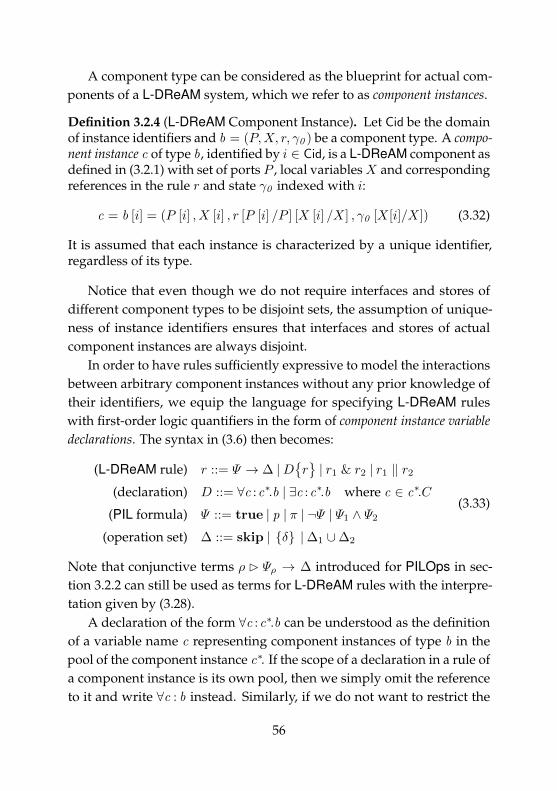
A component type can be considered as the blueprint for actual com-ponents of a L-DReAM system, which we refer to as component instances.

Definition 3.2.4 (L-DReAM Component Instance). Let Cid be the domainof instance identifiers and b = (P,X, r, γ0 ) be a component type. A compo-nent instance c of type b, identified by i ∈ Cid, is a L-DReAM component asdefined in (3.2.1) with set of ports P , local variablesX and correspondingreferences in the rule r and state γ0 indexed with i:

c = b [i] = (P [i] , X [i] , r [P [i] /P ] [X [i] /X] , γ0 [X[i]/X]) (3.32)

It is assumed that each instance is characterized by a unique identifier,regardless of its type.

Notice that even though we do not require interfaces and stores ofdifferent component types to be disjoint sets, the assumption of unique-ness of instance identifiers ensures that interfaces and stores of actualcomponent instances are always disjoint.

In order to have rules sufficiently expressive to model the interactionsbetween arbitrary component instances without any prior knowledge oftheir identifiers, we equip the language for specifying L-DReAM ruleswith first-order logic quantifiers in the form of component instance variabledeclarations. The syntax in (3.6) then becomes:

(L-DReAM rule) r ::= Ψ → ∆ |D{r}| r1 & r2 | r1 ‖ r2

(declaration) D ::= ∀c :c∗.b | ∃c :c∗.b where c ∈ c∗.C



(3.33)

Note that conjunctive terms ρ B Ψρ → ∆ introduced for PILOps in sec-tion 3.2.2 can still be used as terms for L-DReAM rules with the interpre-tation given by (3.28).

A declaration of the form ∀c :c∗.b can be understood as the definitionof a variable name c representing component instances of type b in thepool of the component instance c∗. If the scope of a declaration in a rule ofa component instance is its own pool, then we simply omit the referenceto it and write ∀c : b instead. Similarly, if we do not want to restrict the

56

type of the component instance in the declaration, we simply omit it andwrite ∀c : c∗ (or ∀c if the scope of the variable c is the pool of the samecomponent). ∃c :c∗.b can be interpreted similarly.

Note that ports p and predicates π in PIL formulas can now be para-metric with respect to the instance variables defined in the enclosed dec-laration (e.g. a rule with a declaration ∀c : b can refer to a port p of allcomponent instances c that match the declaration, using the dot notationc.p).

Under the assumption that L-DReAM systems have a finite numberof component instances, each declaration in the rule of a component in-stance can be removed by transforming the rule itself into a combinationof rules (via the & and ‖ operators for the universal and existential quanti-fiers, respectively) where the instance variable is replaced with the actualcomponent instances of the given type in the given pool. We refer to thistransformation as the declaration expansion

⟨⟨r⟩⟩γ

of rule r of a compo-nent instance with state γ =

(σ,C,ΓC

), which is formally defined by the

following rules:⟨⟨Ψ → ∆

⟩⟩γ

= Ψ → ∆⟨⟨∀c :c∗.b

{r}⟩⟩

γ= &

b[i]∈c∗.C

⟨⟨r [b [i] /c]

⟩⟩γ

⟨⟨∀c :c∗

{r}⟩⟩

γ=&∀b

⟨⟨∀c :c∗.b

{r}⟩⟩

γ

⟨⟨∃c :c∗.b

{r}⟩⟩

γ=

n

b[i]∈c∗.C

⟨⟨r [b [i] /c]

⟩⟩γ

⟨⟨∃c :c∗

{r}⟩⟩

γ=

n

∀b

⟨⟨∃c :c∗.b

{r}⟩⟩

γ

⟨⟨r1 & r2

⟩⟩γ

=⟨⟨r1

⟩⟩γ

&⟨⟨r2

⟩⟩γ⟨⟨

r1 ‖ r2

⟩⟩γ

=⟨⟨r1

⟩⟩γ‖⟨⟨r2

⟩⟩γ

(3.34)

where r [b [i] /c] is the rule r after applying the substitution of the instancevariable c with the actual instance b [i].

Example 3.2.3 (Server with n Nodes - declaration expansion). Let us ex-pand Example 3.2.1 and 3.2.2 by considering a scenario where we have avariable pool of Node component instances that one Server instance canuse to handle the computation.

57

We will define the component types Server and Node as follows:

Server = ({accept , reduce, return} , {input , output} , rs, γ0 )

Node = ({receive, return} , {id , data, result} , rn, γ0 )

where we introduced the local variable id to keep track of the identifierof Node instances ready to process their Server ’s input, and the outputvariable is now an array of values (where output [i] represents the i-thelement of the array).

Consider now a system with the same initial configuration describedin Example 3.2.1, where we have one Server instance - Server [0] - and twoNode instances - Node[1],Node[2]. The initial state γ0 of Server [0] will be:

Server [0].γ0 =({input 7→ “hello DReAM!”, output 7→ null} ,{Node[1],Node[2]} , {Node[1].γ0 ,Node[2].γ0}

)

Let us define a fragment r of rule rs of the Server component typemodeling how Node instances are fed input data to be processed usingthe conjunctive style:

r = ∀c :Node{

c.receive B input 6= null ∧ output = null

→ {c.data := split (input , poolSize(this) , c.id)}}

where we extended the split function in order to parametrize the splittingdegree with the number of components in the Server ’s pool (referencedthrough the function poolSize(c)). The declaration expansion of rule runder state Server [0].γ0 is performed by generating a new rule for eachNode instance in the pool of Server and substituting it in place of theinstance variable c:⟨⟨r⟩⟩γ0

= Node[1].receive B input 6= null ∧ output = null

→ {Node[1].data := split (input , poolSize(Server [0]) ,Node[1].id)}&

Node[2].receive B input 6= null ∧ output = null

→ {Node[2].data := split (input , poolSize(Server [0]) ,Node[2].id)}

�

To encompass the additional step of declaration expansion in the de-scription of the behavior of a L-DReAM component, the inference rule

58

(3.17) used to describe the operational semantics of the static version ofthe language needs to be modified accordingly:

∀ci ∈ c.C : ci .γa−→ ci .γ

′ c.γ′ =(c.σ, c.C, {ci .γ′}ci∈c.C

)

a |=c.γ

⟨⟨c.r⟩⟩

c.γc.γ′′ ∈ J

⟨⟨c.r⟩⟩

c.γKa,c.γ (c.γ′)

c.γa−→ c.γ′′

(3.35)

Rule (3.35) now requires that, at each state of a component instance, theproblem of finding an interaction that satisfies its coordination rule issolved after it is reduced to the static, non-parametric case by expandingthe declarations.

Semantics of reconfiguration operations

Since the higher-order language now allows us to express constraintswithout prior knowledge of the individual component instances in a sys-tem, reconfiguration operations are extended in order to allow dynamicvariations in the population of component instances. We thus have threenew operations:

– create (c :b, cs , g)[∆c

]: to create a new component instance of type

b, add it to the pool of component instance cs , and bind it to theinstance variable c within the scope of the operation set ∆c which isthen executed, where g is a generator attribute which can be used todistinguish multiple creation operations with the same parameters;

– delete(c): to delete the component instance c;

– migrate (c, cs): to migrate component instance c to the pool of cs

(removing it from the pool where it previously belonged).

Note that the “create” operation can be written using the short-hand notation create(b, cs , g) when no chained operation has to beperformed after the new instance is created (i.e., create(b, cs , g) ≡create (c :b, cs , g)

[skip

]).

59

To formalize the semantics of the application of the new operationson a component state, let us first define the “binding” support operation:

bind (c, cs) (c.γ) =

{(σ,C ⊕ c,ΓC ⊕ c.γ

)if cs = c(

σ,C,Γ′C)

otherwise(3.36)

where:

– Γ′C = {bind (c, cs) (γi) | γi ∈ ΓC};

– S ⊕ s ≡ S ∪ {s} is the set addition operation.

Note that this operation, which adds c to the pool of cs , is not explicitlyused within L-DReAM rules as its use can produce states where a compo-nent belongs to the pool of two different compounds or to its own pool(which we do not allow).

Having defined the support operation bind, the state transformationinduced by the application of each operation on the component statec.γ =

(σ,C,ΓC

)can now be formalized as follows:

create (c :b, cs , g)[∆c

](c.γ) = (∆c [b[f ] /c])↓γ′ (γ′) (3.37)

where:

– f ∈ Cid is a fresh instance identifier;

– γ′ = bind (b[f ] , cs) (c.γ).

delete(c) (c.γ) =

{(σ,C c,ΓC c.γ

)if c ∈ C(

σ,C,Γ′C)

otherwise(3.38)

where:

– Γ′C = {delete(c) (γi) | γi ∈ ΓC};

– S s ≡ S \ {s} is the set removal operation.

migrate (c, cs) (c.γ) = bind (c, cs) (delete(c) (c.γ)) (3.39)

60

Notice that the generator attribute g has no effect on the semantics ofthe “create” operation (3.37), but contributes to the (implicit) structuralequivalence between operations. Formally:

create (c′1 :b1 , c1 , g1)[∆c′1

]≡ create (c′2 :b2 , c2 , g2)

[∆c′2

]

⇓b1 = b2 and c1 = c2 and g1 = g2

(3.40)

Different choices for this attribute allow to define whether a L-DReAMrule can create multiple instances of the same component type in thesame pool. This can be used to different effect. Consider as an examplethe following rules:

r1 =∀c :c0 .b{true→ {create(b, c0 , 0)}

}

r2 =∀c :c0 .b{true→ {create(b, c0 , c.id)}

}

Assume that c0 hosts two component instances of type b in its pool inits current state γ, respectively with instance identifier equal to 1 and2. The declaration expansion of these two rules in γ according to (3.34)produces:

⟨⟨r1

⟩⟩γ

= true→ {create(b, c0 , 0)}& true→ {create(b, c0 , 0)}⟨⟨r2

⟩⟩γ

= true→ {create(b, c0 , 1)}& true→ {create(b, c0 , 2)}

If we now compute the respective sets of operations to be performed forthe two rules according to (3.10), we get:

J⟨⟨r1

⟩⟩γKγ = {create(b, c0 , 0)}

J⟨⟨r2

⟩⟩γKγ = {create(b, c0 , 1) , create(b, c0 , 2)}

Indeed, the two rules could have been interpreted as follows:

– r1: if c0 hosts at least an instance of type b in its pool, then createanother instance;

– r2: for every instance of type b hosted in the pool of c0 , create a newinstance.

61

The adoption of a snapshot semantics guarantees that component ref-erences are always resolved according to the snapshot, so any operationcan still be carried out even if a delete/migrate operation on the involvedinstance is executed before it. This means, for example, that the execu-tion of the set of operations ∆ = {delete(c) , c′.x := c.x} produces a statewhere c is no longer present and variable c′.x has the same value thatc.x had prior to being deleted, regardless of the order in which the twooperations are resolved.

Conjunctive style in L-DReAM

The full L-DReAM framework relies on the same conjunctive term (3.28)defined for PILOps in section 3.2.2 to build coordination rules using theconjunctive style.

The notion of being “consistent”, which we attributed to conjunctiveterms with operations that only modify the state of the component in-volved in their premise or of any of its descendants, still applies.

Considering the reconfiguration operations introduced in the dy-namic framework, a conjunctive term on component c of the formρc B Ψρc → ∆ρc associated to the rule of component cr is consistent ifits consequence ∆ρc ≡ skip or if it only contains operations δ that verify:

– create (c :b, cs , g)[∆c

]: cs = c, and ρc B true→ ∆c is consistent;

– delete(c): c ∈ Descendants(c)⊕ c;

– migrate (c, cs): c = c, and cs ∈ Descendants(cr )⊕ cr .

Example 3.2.4 (Server with dynamic instantiation of Nodes). Recall theextended scenario presented by Example 3.2.3. We will now integrate thedefinition of the Server and Node component types with their L-DReAMrules using the conjunctive style. Rule rn of the type Node will be essen-tially the same as rk in Example 3.2.2:

rn =receive B data = null ∧ result = null→ skip

&

data 6= nullB true→ {result := f(data), data := null}&

62

return B result 6= null→ {result := null}

Since all the ports and local variables mentioned in rn will be local to eachNode instance, no scoping or quantification is needed.

On the other hand rs will now have to deal with an arbitrary numberof nodes. Recall that the service that we want our Server to provide isthe “character count” function. Let us define rs as the conjunction of thefollowing six sub-rules r1& . . .&r6:

r1 = ∀c :Node{

accept B input = null

→ {output := null, delete(c)}}

Rule r1 implements the output reset of the Server as in the non-parametriccase of Example 3.2.2, but it also deletes every Node instance.

r2 = input 6= null ∧ poolSize(this) = 0B true

→{FOR

(i = 1..length(input)/5

)DO

{

create (c :Node, self, i)[c.id := i

]}}

Rule r2 is completely new to the parametric variant, and it is used tocreate as many Node instances as needed (e.g. in this case one every fivecharacters in input).

r3 = ∀c :Node{

c.receive B input 6= null ∧ output = null

→ c.data := split (input , poolSize(this) , c.id)}

Rule r3 is exactly the same rule as r discussed in Example 3.2.3 describinghow Node components receive input data from the Server .

r4 = ∀c :Node{

reduce B c.return → {output [c.id ] := c.result}}

Rule r4 characterizes how processed data is collected by the Server bycollecting the results in its output local variable.

r5 = return B output 6= null→ {input := null}

Rule r5 is left unchanged from the non-parametric case.

r6 = ∀c :Node{∀c′ :Node

{c.receive B c′.receive → skip

}}

&

∀c :Node{

c.return B reduce → skip}

63

Lastly, r6 enforces strong synchronization between all Node instanceswhen interacting through the receive port, and between the Server andall its nodes through the return and reduce ports (the latter is, in fact,the result of the combination of the second conjunctive term of r6 withr4). �

3.3 Encoding other formalisms

The “loose” characterization of individual components and the freedomto hierarchically compose them makes L-DReAM extremely flexible andcapable of describing a variety of systems and programming paradigms.

Consider for example a labeled transition system (S,L, T ) definedover the states S, labels L and transitions T ⊂ S×L×S. One of the possi-ble modeling of an LTS as a L-DReAM atomic component c = (P,X, r, γ0 )

is the following:

– every label l ∈ L has a corresponding port pl ∈ P ;

– every state s ∈ S has a corresponding local variable xs ∈ X ;

– for every transition 〈si, li, s′i〉 ∈ T there is a ruler =

fi

(xsi ∧ pli →

{xsi := false, xs′i := true

}).

L-DReAM can also be used in an imperative, sequential fashion. To doso, one possibility is to simply add a “program counter” local variable pc

in the store of each component type and conjunct the appropriate pred-icate over it in the requirements of each conjunctive term describing itsbehavior:

rseq = &i

(pi B (Ψ ′i ∧ pc = i)→ ∆i ∪ {pc := pc + 1}) (3.41)

More generally, by using the conjunctive style L-DReAM can be usedas an endogenous coordination language comparable to process calculirelying on a single associative parallel composition operator. Considerfor instance the CCS [40] process P0 defined as the parallel compositionof two processes P1 and P2 that can synchronize over the actions q and u:

P0 = P1 | P2

64

P1 = q.u.0 P2 = q.u.0

where 0 is the inaction. To translate this simple system in L-DReAM wedefine three components ci , each one modeling the process Pi:

c0 =({τ} , ∅, r0,

(∅, {c1 , c2} , {γc1 , γc2 }

))

c1 = ({q , u} , {pc1} , r1, γc1 )

c2 = ({q , u} , {pc2} , r2, γc2 )

where the pool of c0 hosts c1 and c2 .Rules r1, r2 will model a simple sequential process according to (3.41):

r1 = q B (pc1 = 1)→ {pc1 := 2}&

u B (pc1 = 2)→ {pc1 := 3}r2 = q B (pc2 = 1)→ {pc2 := 2}

&

u B (pc2 = 2)→ {pc2 := 3}

The rule r0 of the root component c0 will instead characterize the seman-tics of the CCS parallel composition, which provides that two parallel pro-cesses can synchronize over the matching actions (in this case representedby the interactions {q , q} and {u, u}) causing the system to perform aninternal action τ :

r0 = τ B (q ∧ q) ∨ (u ∧ u)→ skip

Notice that r0 still allows interleaving between c1 and c2 just like for P0.Another way of modeling communicating sequential processes in L-

DReAM is to equip every component with two ports in , out and char-acterize the communication channel (or the action label in CCS) with aspecific local variable chan . This allows to model even more complexsynchronization mechanisms of calculi like π-calculus [41] and one of itsmain features: channel mobility. Let us consider a simple process that wewill call again P0, representing the parallel composition of three processes

65

P1, P2 and P3:

P0 = P1 | P2 | P3

P1 = q(x).x 〈v〉 .0 P2 = q 〈u〉 .0 P3 = u(y).0

The idea is that P1 wants to communicate with P3, but initially can onlycommunicate with P2. Through the output/input pair of actions q 〈u〉and q(x), P2 can send the channel u to P1 which then allows it to send amessage to P3 by binding u to x.

To represent this system in L-DReAM, we will first define the rootcomponent type b0 as before:

b0 =({τ} , ∅, r0,

(∅, ∅, ∅

))

To model the other processes, we will instead define three componenttypes b1 , b2 and b3 :

b1 =({in, out} , {pc, chan, val , x} , r1, γ

10

)

b2 =({in, out} , {pc, chan, val} , r2, γ

20

)

b3 =({in, out} , {pc, chan, y} , r3, γ

10

)

where the initial states γ10 , γ20 and γ30 are respectively:

γ10 =({pc 7→ 1, chan 7→ “q”, val 7→ null, x 7→ null} , ∅, ∅

)

γ20 =({pc 7→ 1, chan 7→ “q”, val 7→ “u”} , ∅, ∅

)

γ30 =({pc 7→ 1, chan 7→ “u”, y 7→ null} , ∅, ∅

)

Rules r1, r2 and r3 will again model sequential processes, but will nowalso handle channel names and value output:

r1 = in B (pc = 1)→ {x := val , chan := x , val := “v”, pc := 2}&

out B (pc = 2)→ {pc := 3}r2 = out B (pc = 1)→ {pc := 2}r3 = in B (pc = 1)→ {pc := 2}

66

The assignments on the chan variable here are used to indicate the chan-nel name associated with the preceding interaction constraint, while theval variable is used to store the channels being passed.

Synchronization and actual value passing is instead implemented byrule r0 of the root component c0 :

r0 = ∃c{∃c′{τ B c.in ∧ c′.out → skip

}}

&

∀c{∃c′{

c.in B c′.out ∧ c.chan = c′.chan → {c.val := c′.val}}}

This rule characterizes both the behavior of the root component type b0

- which performs τ if two instances of any type interact via ports in andout - and the coordination between components in its pool - i.e., for oneto interact with port in there must be another one participating with portout with matching values for their local variables chan . For the sake ofsimplicity, we are omitting further parts of rule r0 to enforce only binarysynchronization between component instances.

L-DReAM can be also used to model capabilities of many other pro-cess algebras relying on more complex and flexible strategies to realizecommunication and coordination between components than simple chan-nels matching. For instance, specifications written with the AbC calculus[1, 2] can be translated to L-DReAM preserving most of the features of thesource language.

In AbC, a system is a set of parallel components equipped with a setof attributes. Communication happens in a broadcast fashion with thecaveat that only components that satisfy some predicates over specificattributes do receive the message given that also the sender satisfies otherpredicates. The core actions of the language that characterize its commu-nication paradigm are the input and output actions:

(input) Π1 (x)

(output) (E)@Π2

where x is a sequence of “placeholders” for the received values and E

is a sequence of expressions representing the values being sent. Π are

67

predicates, which can be defined over attributes only (i.e. for outputactions) or also over received values (i.e. for input actions). A simpleexample of matching input/output actions in AbC could be:

– (x > 1 ∧ color = blue)(x, y): bind two values to variables x, y frommessages having x > 1 and coming from components with attributecolor equal to blue;

– (2, 0)@(color = red): send values 2, 0 to all components with at-tribute color equal to red.

Broadcast communication can be easily implemented in L-DReAM.To maintain uniformity with AbC where actions are defined at compo-nent level, we can adopt the conjunctive style and define two rules thatimplement its input/output actions:

(input) ∀c{∃c′{

c.in B c′.out ∧Π1(c′.E)→{

c.x := c′.E}}}

(output) ∀c{∃c′{

c.out B c′.in ∧Π2 → skip}}

where we assume that:

– the interface of all component types includes two ports in, out ;

– the store of all component types contains local variables describingattributes, values being passed through messages, and the variablesthat are bound to values being passed;

– the predicates Π1,Π2 are equivalent to the respective AbC counter-parts, with the appropriate references to local variables modelingattributes and values being passed.

Going back to the simple example mentioned above, we could translatethe given pair of input/output actions as:

(x > 1 ∧ color = blue)(x, y)

↓∀c{∃c′{

c.in B (c′.out ∧ c′.x > 1 ∧ c′.color = blue)

→{

c.x := c′.x , c.y := c′.y}}}

68

(2, 0)@(color = red)

↓∀c{∃c′{

c.out B (c′.in ∧ c′.color = red)→ skip}}

There are many more nuances to AbC that we are not representinghere, such as the fact that the in action is blocking while the out actionis not. To model this, we need to combine the previously mentionedencoding of the in and out actions with the approach described earlier tosimulate sequential processes in L-DReAM.

69

Chapter 4

The DReAM framework

The L-DReAM framework introduced in Chapter 3 provides a flexible ap-proach to the specification of dynamic and reconfigurable systems. Thelight structure imposed on components and compounds makes it veryclose to a minimal extension to the language used to define its rules,which allows to study it effectively with little overhead. However, thedesign of most “real” systems does not necessarily benefit from the sim-plicity of the adopted formalism. Specialized elements of the languageaddressing common use cases and specific needs can indeed ease the taskof system modeling.

This Chapter presents DReAM (Dynamic Reconfigurable Architecturemodeling) [18, 43], a specialized version of L-DReAM that is equippedwith features supporting effective design of dynamic system architec-tures. DReAM uses the same logic-based modeling language of its “light”counterpart, inheriting its expressive power and flexibility. The systemstructure, however, is no longer a uniform hierarchy of components. In-stead, ti consists of instances of types of components organized in hierar-chies of motifs (see figure 15). Each motif defines how hosted componentsinteract and reconfigure via coordination rules. Thus, a given type of com-ponent can be subject to different rules when it is in a “ring” motif or ina “pipeline” one. Motifs themselves are typed, and each motif instancecan “migrate” from one to another, dynamically changing their hierarchy

70

Motif m1

coordination rule

r1

coordination rule

Map

n1 n2

n4 n5

n3

Pool

c6c7

c8

c9

m5

coordination rule

Motif m2

DReAM System (Motif m0)

r2

r0

Map

n1

n2

n3

c Component instance Component Types n Map NodeMotif Types

Pool

c1c2

c3

m3

c5

c4 m4

Figure 15: Overview of a DReAM system

and thus potentially affecting all the underlying components. Coordina-tion rules in a motif are expressed using the same formalism adopted forL-DReAM rules in (3.33). Component instances can also migrate betweenmotifs, allowing to switch seamlessly coordination style at runtime.

To enhance expressiveness of the different kinds of dynamism, eachmotif is equipped with a map, which is a graph defining the topology ofthe interactions in the motif. To parametrize coordination terms for thenodes of the map, an addressing function @ is provided which defines theposition @(c) in the map of any component instance c associated with themotif. Additionally, each node is equipped with a local memory that canbe accessed by components and used as a shared memory. Maps are alsovery useful to express mobility, in which case the connectivity relation ofthe map represents possible moves of components. Finally, the languageallows to modify maps by adding or removing nodes and edges, as wellas to dynamically create and delete component instances.

71

4.1 Structuring architectures

A DReAM system is made of atomic components, each one characterizedby a behavior, a data store for local variables, and an interface of ports tointeract and coordinate with other components. The system architecturethat realizes their coordination is structured with hierarchies of “motifs”,each representing an independent architecture with its own coordinationrules and data structures for parametrization.

The support for dynamic reconfiguration allows systems to modifytheir architecture at runtime by creating, deleting, and migrating bothcomponents and motifs. This allows to model changes in the populationof entities in the system but also seamless switching of architectural styles.

In this section we will introduce and formally define the entities thatcharacterize the structure of a DReAM system.

4.1.1 Component Types and component Instances

The basic elements of DReAM systems are instances of component types.Component types in DReAM are essentially a mix between L-DReAMcomponent types (Definition 3.2.3) and basic interacting components (Def-inition 3.1.1).

Concretely, DReAM component types are labeled transition systemsequipped with a store (i.e., a set of local variables) and an interface (i.e., a setof ports). Transitions connect control locations of the LTS, and their labelsare transition rules built from a fragment of PILOps (P,X) that we willcall t-PILOps:

(t-PILOps rule) t ::= Φ→ ∆

(PIL atom) Φ ::= idle(P ) | p ∈ P(operation set) ∆ ::= skip | {x := f(X)} |∆1 ∪∆2

(4.1)

where:

– idle(P ) ≡ ∧p∈P ¬p is a notation to represent the PIL monomial

obtained by the conjunction of all the negated ports in P ;

– x ∈ X is a local variable.

72

For the sake of conciseness, we will omit the the operation part of thetransition rule when ∆ = skip (i.e., Φ ≡ Φ→ skip).

The models of the fragment and semantics of operations are the sameas static PILOps defined in section 3.2.1, with the difference that the effectof the application of operations to components states ∆ (γ) is limited tothe valuation function of the component (as DReAM components do nothost other components like L-DReAM compounds, and operation setsassociated to transition only contain assignments).

Having introduced t-PILOps, we can now formally define what a com-ponent type is in DReAM.

Definition 4.1.1 (DReAM Component Type). Let S be the set of all com-ponent control locations, X the set of all local variables, and P the set ofall ports. A component type ct is a transition system ct := (P,X, S, T, γ0 ),where:

– interface P ⊆ P : finite set of ports;

– store X ⊆ X : finite set of local variables;

– S ⊆ S: finite set of control locations;

– T ⊆ S× t-PILOps(P,X)×S: finite set of transitions 〈s, t, s ′〉, wheret ∈ t-PILOps(P,X);

– initial state γ0 ∈ Γ of the form γ0 = (s0 , σ0), with s0 ∈ S andσ0 : X 7→ V is a valuation function for local variables in X .

Each component type has one implicit loop transition 〈s, idle(P ) , s〉 foreach control location s ∈ S. This transition represents the inaction, i.e.,the ability of instances of component type ct of not participating in inter-actions by not changing their state. For the sake of simplicity, we assumethat no transition other than the idle ones are labeled with the PIL formula“idle(P )” (i.e., every non-idle transition is labeled with a port name).

Just like in L-DReAM, component instances are obtained from a com-ponent type by renaming its control locations, ports and local variableswith a unique identifier.

Definition 4.1.2 (DReAM Component Instance). Let Cid be the domainof component identifiers and ct = (P,X, S, T, γ0 ) be a component type.

73

A component instance c of type ct , identified by i ∈ Cid, is obtained byrenaming the set of control locations, ports and local variables of thecomponent type ct with the identifier i, that is:

c , ct [i] = (P [i], X[i], S[i], T [i], γ0 [i]) (4.2)

where:

– the initial state γ0 [i] is obtained from γ0 = (s0 , σ0) by replacingthe initial control location s0 with the renamed s0 [i] ∈ S[i] and byreplacing the domain of σ0 with X[i];

– transitions T [i] are obtained from T by replacing control locations,ports and local variables with their renamed instances:

T [i] ={〈s[i], t[i], s ′[i]〉 |〈s, t, s ′〉 ∈ T, t[i] = t [p[i]/p] [x[i]/x] ∀p ∈ P,∀x ∈ X

}

Without loss of generality, we assume that instance identifiers uniquelyrepresent a component instance regardless of its type.

The state γc of a component instance c is therefore defined as the pairγc = (c.s, c.σ), where c.σ is the valuation function of the variables c.X . Σdenotes the domain of all valuation functions, while we can refer to theset of all possible valuation functions for component instance c with c.Σ.

We use the same notation to denote ports, control locations, states andvariables belonging to a given component instance (e.g. c.p ∈ c.P ). Giventhat, by construction, each instance identifier is uniquely associated to onecomponent instance, we have that sets of ports, control location and localvariables of different component instances are disjoint, i.e. c.P ∩ c′.P = ∅for c 6= c′.

From their “internal” behavioral standpoint, component instances areessentially interacting components (Def. 3.1.1) with transitions possiblyenriched with sets of assignments. As a result, the operational seman-tics of interactions for component instances is defined according to thefollowing rule:

a |= Φ→ ∆ 〈c.s, Φ→ ∆, c.s ′〉 ∈ c.T c.σ′ = ∆ (c.σ)

(c.s, c.σ)a−→ (c.s ′, c.σ′)

(4.3)

74

It is worth pointing out that the hierarchical structuring of L-DReAMcomponents does not apply here, meaning that all DReAM component in-stances are in fact L-DReAM atomic components. The role of compoundsas aggregates of atomic components defining how they interact, coordi-nate and reconfigure, is instead embodied by the specialized concept ofmotif.

Example 4.1.1 (Client-Server architecture with back-end nodes: compo-nent types). Recall the scenario presented in chapter 3 by examples 3.2.1-3.2.4 where we defined a portion of a client-server architecture withServer components receiving data fed to Node components to processand then return the result of the computation. Here we are going tomodel the same general scenario using the DReAM framework. Insteadof focusing only on the “server-side” of the system, now we also modelthe clients querying the service offered by the servers that we defined inthe simple PIL scenario of example 3.1.1.

We start by re-defining the component types Client , Server and Node .

Client component type: clients are simple two-stages automatons thatpost data to servers and then get the result back once ready (figure 16).The operation ∆get associated to the transition from wait to ready handlesthe consumption of the result from the service and generates new data .Additionally, each client has a local variable server to store the identifierof the server queried.

ready wait

post

get → ∆get

data = v0

result = nullserver = null

store:

Figure 16: The Client component type

Server component type: servers accept requests and return results fromClient components, and handle the computation in a distributed fashionby mapping input data to Node instances and reducing the individual re-sults to a single output with operation ∆red (figure 17). The buffer vari-

75

able is an array used to store individual results returned from nodes (i.e.buffer : V 7→ V). Each server keeps also track of the identifier of the clientthat requested the current computation in the local variable client .

wait

busy

linked

done

accept map

reduce → ∆redreturn

input = nullbuffer = ∅output = nullclient = null

store:

Figure 17: The Server component type

Node component type: nodes are modeled with a two-stage automatonthat can receive new data to process, and can return the computationresult when done (figure 18). To ensure that the result is forwarded tothe correct server instance (if more than one is present), each node alsostores the identifier of the server that requested the computation in thelocal variable server .

wait ready

receive

return

data = nullresult = nullserver = null

store:

Figure 18: The Node component type

4.1.2 Motif modeling

A motif characterizes an independent dynamic architecture defined by acoordination rule and parametrized by a data structure called map. Just likecomponent types serve as blueprints for actual executable componentinstances, motif type definitions can be used to create executable motifinstances.

76

Definition 4.1.3 (Motif Type). A motif type mt is a pair mt := (r, µ0),where r is the coordination rule characterizing the interaction and recon-figuration architecture of mt , and µ0 is the initial configuration of the mapassociated to the motif.

A motif can host and coordinate component instances as well as othernested motifs. We refer to the combined set of motifs and componentshosted in another motif as its pool. Every entity hosted in a motif is alsoassociated to its map. A map is a set of locations and a connectivity relationbetween them. It is the structure over which computation is distributedand defines a system of coordinates for hosted components and motifs,which are correlated to locations via an address function. It can represent aphysical structure, such as a geographic map, or some conceptual struc-ture, e.g., the cellular structure of a memory. Additionally, each locationhas a local memory that can written to or read from.

Formally, a map in DReAM is a pair (µ0,F), where µ0 is its initialconfiguration and F is a set of utility functions (e.g. predicates on reacha-bility from one location to another, expressions that return the number ofedges connected to a location, etc). HavingM and C respectively as thedomain of motifs and component instances, the configuration µ of a mapin DReAM is specified as a graph µ =

(N,E, ω,@

), where:

– N is a set of nodes or locations (possibly infinite);

– E is a set of (possibly directed) edges subset of N ×N that definesthe connectivity relation between nodes;

– ω : N 7→ V is a valuation function that associates nodes to values,realizing the map memory;

– @ :M∪ C → N is a (partial) address function binding motifs andcomponents to nodes n ∈ N .

If the map memory is empty, then the only available information for alocation is its name. Otherwise, the memory can be shared by differententities and used for their coordination.

The relation E defines a concept of neighborhood, which is used inmany applications to express coordination constraints or directions for

77

moving components. When these additional topological relations arenot needed and E = ∅, the map can be still used as a simple indexingstructure.

As we mentioned, maps can be used to model a physical environmentwhere components are moving. For example, we can model a discretetwo-dimensional space with an array map N = {(i, j) | i, j ∈ N} × {f, o},where the pairs (i, j) represent coordinates and the symbols f and o standrespectively for free and obstacle. We can model the movement of c, suchthat @(c) = ((i, j), f), to a position (i + a, j + b) provided that there is apath from (i, j) to (i+ a, j + b) consisting of free locations.

A map is also equipped with a set of useful functions F . These mayrange from predicates over the map nodes and edges (e.g., a predicatethat evaluates to true if there exists a sequence of edges connecting twonodes), to selectors that return a specific location having a specific prop-erty (e.g., a function that evaluates to the node with the highest numberof adjacent edges).

Definition 4.1.4 (Motif Instance). Let mt = (r, µ0) be a motif type and Midthe domain of motif identifiers. A motif instance mt [i ] is obtained from mt byrenaming the constituent elements of the initial map configuration mt .µ0

with the identifier i ∈ Mid and all their occurrences in the coordinationrule r:

m , mt [i ] = (r [µ0[i]/µ0] , µ[i]) (4.4)

where µ0[i] = (N [i], E [N [i]/N ] , ω [N [i]/N ] ,@ [N [i]/N ]).The state γm of a motif instance m is the combination of a map config-

uration µ with the sets of hosted motifs M , component instances C, andrespective current states:

γm = (M,C,ΓM ,ΓC , µ) (4.5)

where ΓM = {γmi}mi∈M and ΓC = {γci}ci∈C .

We assume that each motif and component instance is hosted in ex-actly one motif instance, i.e. γm1 .M ∩ γm2 .M = ∅ and γm1 .C ∩ γm2 .C = ∅for any m1 6= m2 .

Like with components, we assume that motif identifiers uniquely sin-gle out motif instances regardless of their type.

78

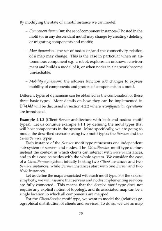
By modifying the state of a motif instance we can model:

– Component dynamism: the set of component instancesC hosted in themotif (or in any descendant motif) may change by creating/deletingor migrating components and motifs;

– Map dynamism: the set of nodes or/and the connectivity relationof a map may change. This is the case in particular when an au-tonomous component e.g. a robot, explores an unknown environ-ment and builds a model of it, or when nodes in a network becomeunreachable;

– Mobility dynamism: the address function µ.@ changes to expressmobility of components and groups of components in a motif.

Different types of dynamism can be obtained as the combination of thesethree basic types. More details on how they can be implemented inDReAM will be discussed in section 4.2.2 where reconfiguration operationsare introduced.

Example 4.1.2 (Client-Server architecture with back-end nodes: motiftypes). Let us continue example 4.1.1 by defining the motif types thatwill host components in the system. More specifically, we are going tomodel the described scenario using two motif types: the Service and theClientService types.

Each instance of the Service motif type represents one independentsub-system of servers and nodes. The ClientService motif type definesinstead the context in which clients can interact with Service instances,and in this case coincides with the whole system. We consider the caseof a ClientService system initially hosting two Client instances and twoService instances, while Service instances start with one Server and twoNode instances.

Let us define the maps associated with each motif type. For the sake ofsimplicity, we will assume that servers and nodes implementing servicesare fully connected. This means that the Service motif type does notrequire any explicit notion of topology, and its associated map can be asingle location to which all components are mapped.

For the ClientService motif type, we want to model the (relative) ge-ographical distribution of clients and services. To do so, we use as map

79

for the motif a graph with N locations, to which Client and Service in-stances are assigned, linked by edges that represent the notion of topolog-ical proximity in the connectivity network. For the initial configurationµ0 = (N,E, ω,@) we have:

µ0 = ({n0, . . . , n3} , {(n0, n2) , (n1, n2) , (n1, n3)} , ∅,@0)

that isN is a set of 4 locations andE is a set of 3 edges connecting them asin figure 19. The initial address function @0 maps clients and services insuch a way that each client’s location is linked with at least one locationmapped to a service:

@0 = {Client1 7→ n0,Client2 7→ n1,Service1 7→ n2,Service2 7→ n3}

The support functions F of the map only includes a predicate

n0

n2 n3

Client1 Client2n1

Service1 Service2

ClientService map

Figure 19: The initial configuration of the map of ClientService motif type

isEdge(n1, n2

)that evaluates to true only if (n1, n2) ∈ E. This predi-

cate will allow us to test “reachability” of services by clients when wedefine the coordination rules of the ClientService motif type.

4.2 The DReAM coordination language

The coordination language modeling interactions between componentsis, for the most part, independent from the abstract system structure. Con-sequently, the coordination language introduced in section 3.2.3 is sharedbetween L-DReAM and DReAM.

80

Given the domain of ports P and the set of all possible system statesΓ , the DReAM coordination language is therefore obtained from (3.33) byreplacing the generic compound c∗ with the motif m in the scope of thedeclarations:

(DReAM rule) r ::= Ψ → ∆ |D{r}| r1 & r2 | r1 ‖ r2

(declaration) D ::= ∀m :ms .mt | ∃m :ms .mt | ∀c :ms .ct | ∃c :ms .ct



(4.6)where declarations define the context of the associated rule by declaringquantified (∀|∃) variables for motifs (m) and components (c) associatedto instances of a given type (mt and ct , respectively) hosted in a “scope”motif ms .

Note that predicates π now include map functions in F with Booleancodomain (e.g., the isEdge

(n1, n2

)predicate used in example 4.1.2) and

can use other map functions in equality/inequality relations (e.g., hav-ing defined the function tail(m) that returns the last location in a mapmodeling an ordered sequence of nodes, we can define a predicate thatis satisfied when the component c is located in this last location as@(c) = tail(m)).

A DReAM coordination rule is well formed if all motifs and componentvariables appearing in the scope of declarations, PIL formulas and associ-ated operations, are defined in a declaration. From now on, we will onlyconsider well formed terms.

Just like in L-DReAM, given a system state, a DReAM rule can betranslated to an equivalent one by performing a declaration expansion step,which expands the quantifiers and replaces variables with actual motifand component instances.

4.2.1 Declaration expansion for coordination terms

Given that DReAM systems host a finite number of motif and componentinstances, first-order logic quantifiers can be eliminated by enumeratingevery one of them according to the type specified in each declaration. We

81

thus define the declaration expansion⟨⟨r⟩⟩γm

of rule r in motif m understate γm by adapting rules (3.34) as follows:

⟨⟨Ψ → ∆

⟩⟩γm

= Ψ → ∆⟨⟨∀m :ms .mt

{r}⟩⟩

γm= &

mt[i]∈γms .M

⟨⟨r [ct [i ]/c]

⟩⟩γm

⟨⟨∃m :ms .mt

{r}⟩⟩

γm=

n

mt[i]∈γms .M

⟨⟨r [mt [i ]/m]

⟩⟩γm

⟨⟨∀c :ms .ct

{r}⟩⟩

γm= &

ct[i]∈γms .C

⟨⟨r [ct [i ]/c]

⟩⟩γm

⟨⟨∃c :ms .ct

{r}⟩⟩

γm=

n

ct[i]∈γms .C

⟨⟨r [ct [i ]/c]

⟩⟩γm

⟨⟨r1 & r2

⟩⟩γm

=⟨⟨r1

⟩⟩γm

&⟨⟨r2

⟩⟩γm⟨⟨

r1 ‖ r2

⟩⟩γm

=⟨⟨r1

⟩⟩γm‖⟨⟨r2

⟩⟩γm

(4.7)

where:

– ms is either a descendant of m or they coincide;

– r [mt [i ]/m] is the substitution of the motif variable m with the actualinstance mt [i ] in rule r;

– r [ct [i ]/c] is the substitution of the component variable c with theactual instance ct [i ] in rule r.

For the sake of conciseness, (4.6) and (4.7) do not mention additionalnotations that can be used to ease declaration writing. For instance, ex-plicit reference to the motif hosting the instance variable can be omit-ted when the term is associated to the motif itself (otherwise referencedthrough the this keyword). Similarly, if the rule has to apply to groupsof instances regardless of their type, the component type can be omittedin the declaration.

By applying (4.7) exhaustively under a given system state, any rulecan be transformed into an equivalent one only involving actual motifsand component instances free of declarations. Notice that this transfor-mation is only practically feasible at runtime when the exact hierarchy ofcomponent and motif instances is known.

82

4.2.2 Reconfiguration operations

In addition to the “assignment” operation already introduced for PILOpsin section 3.2.1, DReAM supports more complex reconfiguration opera-tions which enable component, map and mobility dynamism by allowingtransformations of a motif configuration at run-time. Some of them arenatural extensions of the ones introduced for L-DReAM in section 3.2.3,while others are entirely new and exclusive to DReAM.

We will now list all the main operations that enable reconfigurationcapabilities breaking them down into three classes of dynamism:

1. Motif dynamism can be realized using the following statements:

– create(m :mt ,ms , n, g)[∆m

]: to create a new motif instance of

type mt at node n of the map of motif ms , binding it to thevariable m within the scope of the operation ∆m , which isthen executed;

– delete(m): to delete motif instance m (and all its descendants).

2. Component dynamism can be realized using the following state-ments:

– create(c :ct ,ms , n, g)[∆c

]: to create a component instance of

type ct at node n of the map of motif ms , binding it to thevariable c within the scope of the operation ∆c , which is thenexecuted;

– delete(c): to delete component instance c.

3. Map dynamism can be realized using the following statements:

– addNode(n,ms , g)[∆n

]: to create a new location in the config-

uration of the map of motif ms , binding it to variable n withinthe scope of the operation ∆n, which is then executed;

– rmNode(n,ms): to remove node n from the configuration of themap of motif ms , along with incident edges, mapped motifsand components;

83

– addEdge(n1, n2,ms): to add the edge (n1, n2) to the configura-tion of the map of motif ms ;

– rmEdge(n1, n2,ms): to remove the edge (n1, n2) from the con-figuration of the map of motif ms .

4. Mobility dynamism can be realized using the following statements:

– move(m, n): to change the position of motif instance m to noden in the map of motif ms ;

– move(c, n): to change the position of component instance c tonode n in the map of motif ms .

5. Dynamic changes of architectural constraints can be realized withthe following statements:

– migrate(m,ms , n): to move a motif instance m to node n in themap of the motif instance ms ;

– migrate(c,ms , n): to move a component instance c to node n inthe map of the motif instance ms .

where g is a generator attribute that is used to discriminate multiple oper-ations with the same parameters as in the L-DReAM “create” operation(described in section 3.2.3).

Semantics of reconfiguration operations

The application of the listed reconfiguration operations on the state of amotif produces a new state. Let m be a motif and m.γ = (M,C,ΓM ,ΓC , µ)

be its state, where µ =(N,E, ω,@

)is the configuration of the associated

map. To formalize the transformation induced by the application of eachdifferent reconfiguration operation on the state m.γ, let us first definethe semantics of the application of the support “binding” operations asfollows:

bind (m,ms , n) (m.γ) =

{(M ⊕m, C,ΓM ⊕m.γ0 ,ΓC , µ

′) if ms = m

(M,C,Γ′M ,ΓC , µ) otherwise(4.8)

84

where:

– µ′ =(N,E, ω,@ [m 7→ n]

);

– Γ′M = {bind (m,ms , n) (γi) | γi ∈ ΓM};

– S ⊕ s ≡ S ∪ {s} is the set addition operation.

bind (c,ms , n) (m.γ) =

{(M,C ⊕ c,ΓM ,ΓC ⊕ c.γ0 , µ

′) if ms = m


where:

– µ′ =(N,E, ω,@ [c 7→ n]

);

– Γ′M = {bind (c,ms , n) (γi) | γi ∈ ΓM}.

bindNode(n,ms) (m.γ) =

{(M,C,ΓM ,ΓC , µ

′) if ms = m


where:

– µ′ =(N ⊕ n,E, ω,@

);

– Γ′M = {bindNode(n,ms) (γi) | γi ∈ ΓM}.

As already mentioned for L-DReAM, the bind and bindNode operations areintroduced to simplify the presentation of the semantics of more complexreconfiguration operations, which we will now detail.

create(m :mt ,ms , n, g)[∆m

](m.γ) = (∆m [mt [f ] /m])↓γ′m (γ′m) (4.11)

where:

– f ∈ Mid is a fresh motif instance identifier;

– γ′m = bind (mt [f ] ,ms , n) (m.γ).

85

delete(m) (m.γ) =

{(M m, C,ΓM m.γ,ΓC , µ

′) if m ∈M(M,C,Γ′M ,ΓC , µ) otherwise

(4.12)

where:

– µ′ =(N,E, ω,@ [m 7→ ⊥]

), i.e., remove m from the domain of @;

– Γ′M = {delete(m) (γi) | γi ∈ ΓM};

– S s ≡ S \ {s} is the set removal operation.

create(c :ct ,ms , n, g)[∆c

](m.γ) = (∆c [ct [f ] /c])↓γ′m (γ′m) (4.13)

where:

– f ∈ Cid is a fresh component instance identifier;

– γ′m = bind (ct [f ] ,ms , n) (m.γ).

delete(c) (m.γ) =

{(M,C c,ΓM ,ΓC c.γ, µ′) if C ∈ C(M,C,Γ′M ,ΓC , µ) otherwise

(4.14)

where:

– µ′ =(N,E, ω,@ [c 7→ ⊥]

), i.e., remove c from the domain of @;

– Γ′M = {delete(c) (γi) | γi ∈ ΓM}.

addNode(n,ms , g)[∆n

](m.γ) = (∆n [n′/n])↓γ′m (γ′m) (4.15)

where:

– n′ is a new map location;

– γ′m = bindNode(n′,ms) (m.γ).

rmNode(n,ms) (m.γ) =

{(M ′, C ′,ΓM ′ ,ΓC′ , µ′) if ms = m


86

where:

– the map configuration µ′ is obtained from µ by: removing node n,removing all edges incident to n, removing the valuation for n fromω, and keeping only the the mappings towards location differentfrom n in the addressing function @:

µ′ =(N n, {(n1, n2) | (n1, n2) ∈ E : n1 6= n ∧ n2 6= n} ,

ω [n 7→ ⊥] , {(e 7→ ni) | (e 7→ ni) ∈ @ : ni 6= n})

– M ′ = M \ {m | m ∈M : @(m) = n};

– C ′ = C \ {c | c ∈ C : @(c) = n};

– Γ′M = {rmNode(n,ms) (γi) | γi ∈ ΓM}.

addEdge(n1, n2,ms) (m.γ) =

{(M,C,ΓM ,ΓC , µ

′) if ms = m


where:

– µ′ =(N,E ⊕ (n1, n2) , ω,@

)if n1, n2 ∈ N , otherwise µ′ = µ;

– Γ′M = {addEdge(n1, n2,ms) (γi) | γi ∈ ΓM}.

rmEdge(n1, n2,ms) (m.γ) =

{(M,C,ΓM ,ΓC , µ

′) if ms = m


where:

– µ′ =(N,E (n1, n2) , ω,@

)if n1, n2 ∈ N , otherwise µ′ = µ;

– Γ′M = {rmEdge(n1, n2,ms) (γi) | γi ∈ ΓM}.

move(m, n) (m.γ) =

{(M,C,ΓM ,ΓC , µ

′) if m ∈M(M,C,Γ′M ,ΓC , µ) otherwise

(4.19)

87

where:

– µ′ =(N,E, ω,@ [m 7→ n]

)if n ∈ N , otherwise µ′ = µ;

– Γ′M = {move(m, n) (γi) | γi ∈ ΓM}.

move(c, n) (m.γ) =

{(M,C,ΓM ,ΓC , µ

′) if c ∈ C(M,C,Γ′M ,ΓC , µ) otherwise

(4.20)

where:

– µ′ =(N,E, ω,@ [c 7→ n]

)if n ∈ N , otherwise µ′ = µ;

– Γ′M = {move(c, n) (γi) | γi ∈ ΓM}.

migrate(m,ms , n) (m.γ) = bind (m,ms , n) (delete(m) (m.γ)) (4.21)

migrate(c,ms , n) (m.γ) = bind (c,ms , n) (delete(c) (m.γ)) (4.22)

4.2.3 Disjunctive and Conjunctive styles in DReAM

As we have seen, DReAM inherits the core coordination language to de-fine its rules from L-DReAM. As such, the two frameworks naturallyshare also the different approaches on system specification that we calleddisjunctive and conjunctive presented in sections 3.1.4 and 3.2.2. Notably,the coordination language defined in (4.6) is enriched with the same con-junctive term formalized in definition 3.2.2.

The notion of “consistency”, introduced for conjunctive PILOps terms,is also extended to encompass the richer set of reconfiguration operationsand the different system structure. That is, having ρc be either a port c.p

or a predicate π (c.X), we consider a conjunctive term ρc B Ψρc → ∆ρc tobe consistent if its consequence ∆ρc is equal to skip, or if it only containsoperations δ that do not modify the state of components different from c

nor their addressing in the relevant map. Concretely, this allows ∆ρc toinclude any operation that modifies the state of c and of its ancestors aslong as it does not delete, move, or migrate another component instance,nor it performs an assignment on one of its local variables.

A DReAM rule for motif m is written using the conjunctive style bycombining consistent conjunctive terms with the & operator.

88

Example 4.2.1 (Client-Server architecture with back-end nodes: coordi-nation rules). In example 4.1.2 we described the general architectureof the system and the initial configuration of the map for motif typeClientService. Now we define the coordination rules that realize the in-teraction patterns described qualitatively in example 4.1.1 adopting theconjunctive style.

Let us start with rule rcs of the ClientService motif type. The interac-tions that need to be modeled are of two kinds, both involving a Clientinstance and a Server instance: one that starts a task on the client’s data,and one that transfers the results of the task back to the client. We can sep-arate rcs into two sub-rules each modeling the two kinds of interactionslisted:

– rule r1cs, which models the strong synchronization between clients

and servers that are mapped to connected locations in the map al-lowing the former to send data to process to the latter:

r1cs =∀c :Client

{∃s :Service.Server

{

c.post B s.accept ∧ isEdge(@(c) ,@(s)

)

→ {c.server := s.id}}}

&

∀s :Service.Server{∃c :Client

{

s.accept B c.post ∧ isEdge(@(c) ,@(s)

)

→ {s.client := c.id , s.input := c.data}}}

– rule r2cs, which models the strong synchronization between clients

and servers that are mapped to connected locations in the map al-lowing the former to receive the results of the computation fromthe latter:

r2cs =∀c :Client

{∃s :Service.Server

{

c.get B s.return ∧ isEdge(@(c) ,@(s)

)∧ (s.id = c.server)

→ {c.result := s.output}}}

&

∀s :Service.Server{∃c :Client

{

s.return B c.get ∧ isEdge(@(c) ,@(s)

)∧ (c.id = s.client)

→ skip}}

89

Notice that in the declaration of the component variable s we used acompressed notation that implicitly defines the scope of the variable inany Service motif instance:

∀c :mt .ct{r}≡ ∀m :mt

{∀c :m.ct

{r}}

∃c :mt .ct{r}≡ ∃m :mt

{∃c :m.ct

{r}}

To ensure that the initial synchronization between a client and a serverdoes not involve more than one instance of each, we also add a rule ofthe form:

r3cs = atMost(1,Client .post) & atMost(1,Service.Server .accept)

where atMost(k,mt .ct .p) is a macro notation for a rule that is satisfied byinteractions in which there are at most k component instances of type ctin a motif of type mt participating with port p:

atMost(k,mt .ct .p) , ∀m :mt

{∀c0 , . . . , ck :m.ct

{

c0 .p B∨

i,j∈[0..k],i6=jci = cj ∨

∨

i∈[1..k]

¬ci .p → skip

}}

(4.23)By combining these three sub-rules we obtain rcs = r1

cs & r2cs & r3

cs.To complete the specification, we need to define the coordination rule

rs for motif type Service. Since the interactions involve one Server com-ponent instance and some Node component instances in a two-phase ren-dezvous synchronization, we can define rs using the same “structure” weused for rcs, i.e., dividing it into two sub-rules:

– rule r1s , which models the strong synchronization between servers

and nodes, allowing the former to send data to process to the latter:

r1s =∀s :Server

{∃n :Node

{

s.map B n.receive → skip}}

&

∀n :Node{∃s :Server

{

n.receive B s.map

→ {n.server := s.id ; n.data := s.input}}}

90

where, for the sake of simplicity, we have assumed that serverstransfer all the input data to each node.

– rule r2s , which models the strong synchronization between servers

and nodes allowing the former to receive the results of the compu-tation from the latter:

r2s =∀s :Server

{∃n :Node

{

s.reduce B n.return → {s.buffer [n.id ] := n.result}}}

&

∀n :Node{∃s :Server

{

n.return B s.reduce ∧ (n.server = s.id)→ skip}}

We apply similar restrictions as the ones in r3cs on the number of servers

allowed to participate in an interaction:

r3s = atMost(1,Server .map) & atMost(1,Server .reduce)

which combined with the other two sub-rules produces rs = r1s & r2

s & r3s .

4.2.4 Operational semantics

As described in 4.1.2, motifs are equipped with rules r of the coordinationlanguage which are used to compose motif and component instancesassigned to them and regulate their interactions. A motif instance m

can evolve from state γm to state γ′′m by performing a transition labeledwith the interaction a and characterized by the application of the set ofoperations J

⟨⟨r⟩⟩γm

Ka,γm iff a |=⟨⟨r⟩⟩γm

. Formally this is encoded by thefollowing inference rule:

a |=γm

⟨⟨r⟩⟩γm

γma−→ γ′m γ′′m ∈ J

⟨⟨r⟩⟩γm

Ka,γm (γ′m)

γma

γ′′mm = (r, µ0)

(4.24)where:

– recall that rule (4.3) defines the semantics of individual componentinstances; γm

a−→ γ′m expresses the capability of the motif m to

91

evolve to state γ′m when its hosted motif and component instancesevolve with a:

∀γmi∈ ΓM : γmi

aγ′mi

∀γc ∈ ΓC : γca−→ γ′c

(M,C,ΓM ,ΓC , µ)a−→(M,C,

{γ′mi

}M,{γ′ci}C, µ) (4.25)

– J⟨⟨r⟩⟩γm

Ka,γm (γ′m) is the set of motif configurations obtained accord-ing to (3.10) and (3.13) by applying the operations ∆ = J

⟨⟨r⟩⟩γm

Ka,γmto the motif configuration γ′m .

Rules (4.24-4.25) can be intuitively understood as follows: a motif m

evolves through interaction a, provided it satisfies its coordination rule,if all its hosted motifs and component instances can also evolve througha making m reach an intermediate state γ′m ; as a consequence, the finalstate γ′′m reached by m is obtained by applying the operations in its coor-dination rule evaluated in its initial state to the intermediate state γ′m .

Definition 4.2.1 (DReAM system). Let Tm and Tc be respectively aset of motif types and component types. A DReAM system is a tuple(Tm ,Tc ,mr ) where mr is the root motif.

The operational semantics of a DReAM system is defined by the infer-ence rule (4.24) applied to the state γmr

of the root motif mr .

4.3 Example systems

We will now present how some simple application scenarios can be mod-eled using the DReAM coordination language.

4.3.1 Coordinating flocks of interacting robots

Consider a system with N robots moving in a square grid, each one withgiven initial location and initial movement direction as represented infigure 20. Robots are equipped with a sensor that can detect other peerswithin a specific range ρ and assess their direction: when this happens,the robot changes its own direction accordingly.

92

We require that robots maintain a timestamp of their last interactionwith another peer: when two robots are within the range of their sensors,their direction is updated with the one having the highest timestamp. Forthe sake of simplicity we also assume that the grid is, in fact, a torus withno borders.

x

r5

0

1

2

3

4

5

0 1 2 3 4 5

r8 r9

r2r1 r3

r4 r6

r7

y

nodeaddress

Figure 20: Initial system configuration for grid size s = 6

To model these robots in DReAM we will define a Robot componenttype as the one represented in figure 21. Each Robot maintains a localclock that is incremented by 1 through an assignment operation everytime an instance interacts with port tick .

93

s0 tick → {clock := clock + 1}clock = 0range = ρts = 0dir = [dx, dy]

store:

Figure 21: The Robot component type

A motif that realizes the described scenario can be defined with theconjunction of two coordination terms: one that enforces synchronizationbetween every Robot instance through port tick allowing informationexchange when possible, and another that enables all Robot instancesperforming a tick to move:

r = ∀c :Robot{

c.tick B true→ {move(c,@(c) + c.dir)}}

&

∀c1 , c2 :Robot{

c1 .tick B c2 .tick

→ IF(c1 6= c2 ∧@(c1 )↔ @(c2 ) < c1 .range

∧ (c1 .ts < c2 .ts ∨ (c1 .ts = c2 .ts ∧ c1 < c2 )))THEN

{c1 .dir := c2 .dir , c1 .ts := c1 .clock

}}

where:

– we use a map whose nodes are addressed via size-two integer ar-rays [x, y];

– we are using a n1 ↔ n2 function that returns the euclidean distancebetween two points in an n-dimensional space;

– in the inequality c1 < c2 we use instance variables c1 , c2 in placeof their respective integer instance identifiers.

The coordination rule r, which adopts the conjunctive style, can be intu-itively understood breaking it into two parts:

1. every robot c can interact with its port c.tick , and if it does it alsomoves according to its stored direction c.dir ;

94

2. for every robot c1 to interact with its port c1 .tick , every robot c2

must also participate in the interaction with its port c2 .tick (i.e.interactions through port tick are strictly synchronous). Further-more, for every pair of distinct (c1 6= c2 ) robots c1 , c2 interactingthrough their respective tick ports: if they are closer than a givenrange (@(c1 ) ↔ @(c2 ) < c1 .range) and either c1 has updated itsdirection less recently (c1 .ts < c2 .ts) or they have updated theirdirections at the same time but c2 has a higher instance identifier(c1 .ts = c2 .ts ∧ c1 < c2 ), then c1 will update its direction andtimestamp using c2 ’s.

Notice that if the direction of a robot is updated at a given time, the robotwill move according to this new direction only during the next clock cyclebecause of the adopted snapshot semantics.

Since all robots synchronize on the same “clock”, many of them mightupdate their respective directions differently at the same time: adding the“tiebreaker” on the instance identifier when timestamps are equal allowsdata exchange even in these cases.

Multiple updates of the direction of a robot c can still happen whenmore than one peer with higher timestamp (or equal timestamp, buthigher instance identifier) is within its range: this event does not affectthe assignment on c.ts , which only depends on the clock, but ultimatelycauses the direction of c to be updated nondeterministically with one ofthe directions of the robots in range according to the semantics of theapplication of operation sets (3.13).

4.3.2 Coordinating flocks of robots with stigmergy

We consider a variant of the previous problem by using stigmergy [51].Instead of letting robots sense each other, we will allow them to “mark”their locations with their direction and an associated timestamp. In thisway, each time a robot moves to a node in the map it will either updateits direction with the one stored in the node or update the one associatedwith the node with the direction of the robot (depending on whether thetimestamp stored in the node memory is more recent than the last time

95

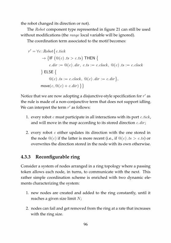
the robot changed its direction or not).The Robot component type represented in figure 21 can still be used

without modifications (the range local variable will be ignored).The coordination term associated to the motif becomes:

r′ = ∀c :Robot{

c.tick

→{IF(@(c) .ts > c.ts

)THEN

{

c.dir := @(c) .dir , c.ts := c.clock , @(c) .ts := c.clock}ELSE

{

@(c) .ts := c.clock , @(c) .dir := c.dir},

move(c,@(c) + c.dir)}}

Notice that we are now adopting a disjunctive-style specification for r′ asthe rule is made of a non-conjunctive term that does not support idling.We can interpret the term r′ as follows:

1. every robot c must participate in all interactions with its port c.tick ,and will move in the map according to its stored direction c.dir ;

2. every robot c either updates its direction with the one stored inthe node @(c) if the latter is more recent (i.e., if @(c) .ts > c.ts) oroverwrites the direction stored in the node with its own otherwise.

4.3.3 Reconfigurable ring

Consider a system of nodes arranged in a ring topology where a passingtoken allows each node, in turns, to communicate with the next. Thisrather simple coordination scheme is enriched with two dynamic ele-ments characterizing the system:

1. new nodes are created and added to the ring constantly, until itreaches a given size limit N ;

2. nodes can fail and get removed from the ring at a rate that increaseswith the ring size.

96

empty full

in → ∆pl

init → ∆pl

out

payload = nullbuffer = null

store:

Figure 22: The Node component type

The Node component type is represented in figure 22. Each Node hastwo local variables: payload , that holds the next value to send, and buffer ,that stores the last value received. The payload variable is initialized viathe operation ∆pl associated to the transitions that change the controllocation of a Node from empty to full , which will contain an assignmentof the form payload := v, where v is a value that the Node wants to transferto its neighbor. The out and in ports are used intuitively to model the sendand receive actions that a Node can perform with its neighbors in the ring,while the init port is used to handle more conveniently the bootstrappingof the system when all nodes are in the initial empty control location.

The motif that will model the system needs to be equipped with anappropriate map to represent the ring topology of interest, which is essen-tially a cyclic directed graph with just one cycle. The functions associatedto this kind of map will have to allow adding and removing map locationsby also updating the set of edges in order to preserve the initial propertiesof the graph. Furthermore, we assume that initially each Node instancehas a one-to-one correspondence with a location. Figure 23 illustrates agraphical representation of the ring with four Node instances, where thedata flow and relationship between component instances and locationsof the map are highlighted in green. Having these ingredients, we candefine a coordination term r that realizes the described behavior adoptingthe conjunctive style. This allows us to be compositional in our designprocess, so we will make use of this advantage and divide the problem ofdefining r into three simpler sub-problems.

First, we will model how the ring grows and shrinks as new Node

instances are created and removed. As we previously mentioned, we

97

out

in

in

out

outin

out in

N1 @N1

N4

N3

N2

@N2

@N3

@N4

Figure 23: A representation of a ring with four Node instances and the corre-sponding map

will design the system in such a way that one new Node is added tothe ring map as long as its size is less than N . At the same time, anyNode instance in the system can terminate and get removed from thering with probability D

(ring.size

N

)2, where D ∈ [0, 1]. When this happens,

the ring will automatically reconfigure to preserve the overall structureas illustrated in figure 24. To keep the example simple, we encode theinformation required to model this behavior directly within the motif: theconstants N andD will be statically defined within the coordination termr, and the current ring size will be obtained from a property of the map(i.e., the number of its locations). We can encode this behavior with thefollowing rule:

r1 = ring .size < N B true

→{addNode(n, this, g)

[create(Node, this, n)

]}

&

∀c :Node{rand < D (ring .size/N)

2 B true

→ {rmNode(@(c) , this)}}

where rand ∈ [0, 1] is a random number.Next, we will define how components interact and transfer data. Com-

munication is binary between neighboring nodes in the ring: a Node ni

98

out

in

in

out

outin

out in

N1 @N1

N4

N3

N2

@N2

@N3

@N4

(a) N3 and the location @(N3) are deleted

out

in

outin

out in

N1 @N1

N4

N2

@N2

@N4

(b) and the map reconfigures to pre-serve the ring

Figure 24: How the system handles Node deletion

can send data to a Node nj only if the edge (@(ni) ,@(nj )) belongs to thering map (which we express with the predicate isEdge

(ni ,nj

)). Addition-

ally, the node sending data and the one receiving it have to participate inthe interaction with ports out and in , respectively. We can encode theseconstraints in the following way:

r2 = ∀c1 , c2 :Node{

c1 .out B isEdge(c1 , c2

)∧ c2 .in → skip

}

&

∀c1 , c2 :Node{

c1 .in B isEdge(c2 , c1

)∧ c2 .out

→ {c1 .buffer := c2 .payload}}

Lastly, we need to handle the transient situations when all nodes arein the empty (initial) control location. We can model a system with asingle passing token by defining a coordination term that allows just oneNode instance to perform an init provided that every other Node instanceis empty and stays idle :

r3 = ∀c1 , c2 :Node{

c1 .init B c1 = c2 ∨ (c2 .empty ∧ c2 .idle )→ skip}

This term will come into play after the creation of the very first Node

99

instance in the ring and in the event that the Node instance holding thetoken gets removed from the ring.

The overall coordination rule r of the motif modeling the system willbe the conjunction of the given rules:

r = r1 & r2 & r3

4.3.4 Simple platooning protocol for automated high-ways

Platooning protocols aim at addressing the problem of coordinating col-lections of vehicles autonomously while guaranteeing some desired prop-erties (e.g., human safety, fuel efficiency, traffic intensity, and so on). Herewe will model a simple platooning protocol inspired by [10, 30].

Let us consider a scenario where we have a one-way road where au-tonomous cars move. Cars are organized in platoons, i.e., groups of oneor more cars next to one-another proceeding at the same speed. Each pla-toon has one leader car, that is the car leading the platoon. While moving,a platoon can:

– join another platoon, if the distance between their leading/trailingcars is below a certain threshold d: after the platoons join, the cruis-ing speed is set to the value of the slower one (i.e., the one that wason the front);

– split into two separate platoons, if for instance a car has to decreaseits speed in order to exit the road via an intersection: the speed ofthe platoon in front is increased by a factor ∆s, while the one in theback is decreased by the same factor ∆s.

To model the system we define two motif types: the Road and thePlatoon . The Platoon motifs define how cars bound to the specific motifinstance move and keep track of their relative position within the platoon.One Road motif instance represents the whole system, and coordinatesall the Platoon instances it hosts.

We model cars as component instances of the type Car . A car keepstrack of its speed and position on the road, and has an interface towards

100

other cars to signal the initiation of a joining/splitting procedure, theacknowledgment of another car’s joining/splitting, and the completionof either procedures. Figure 25 provides a complete representation of theCar component type.

s0 sbsa

initSplit

closeSplit

ackSplit

initJoin

finishJoin

ackJoin pos = π0

speed = v0

store:

Figure 25: The Car component type

The Platoon motif type is characterized by a map that models the trainof cars using an indexed linked list, where each location is referenced by aunique integer address and is meant to be occupied by one car (figure 26).

0 1 2 3

Car0 Car1 Car2 Car3

pool

map

leader tail

Figure 26: A representation of the Platoon map

The coordination rule rP associated to the motif in this simple scenariodefines:

1. how each car in the platoon updates its position based on its currentspeed;

2. the requirement of having more than 1 car for any of them to triggerthe splitting of the platoon;

101

3. the synchronization between all cars in the platoon when the join-ing/splitting maneuvers are performed.

This can be encoded in the DReAM coordination language using the con-junctive style as follows:

rP = ∀c :Car{true→ {c.pos := c.pos + c.speed ×∆t}

}(4.26)

&

∀c :Car{

c.initSplit B poolSize(this) > 1

∧ leader(this) 6= c ∧ rand(0, 1) < psplit → skip}

(4.27)

&

∀c :Car{∀c′ :Car

{c.ackJoin B c′.ackJoin → skip

}}(4.28)

&


{c.initJoin B c′.initJoin → skip

}}(4.29)

&


{c.finishJoin B c′.finishJoin → skip

}}(4.30)

&

∀c :Car{∃c′ :Car

{c.ackSplit B c′.initSplit → skip

}}(4.31)

&


{c.initSplit B c′.ackSplit ∨ c = c′ → skip

}}

(4.32)

where:

– poolSize(m) is a function that returns the number of componentsand motifs hosted in m ;

– leader(m) ∈ F is a function of the Platoon map that returns theentity assigned to the first position (0-indexed) of the map of motifm ;

– rand(0, 1) is a function that returns a random number between 0

and 1;

102

– psplit is the probability that a car can initiate a splitting maneuverat any given time (for simplicity we are assuming this being a pa-rameter of the system).

Sub-rules (4.26-4.27) directly implement the policies described in 1-2. Sub-rules (4.28-4.30) force the symmetric synchronization of all the cars in theplatoon when a join maneuver is initiated, acknowledged, or completed.Lastly (4.31-4.32) prescribe a splitting platoon to have all its cars but oneacknowledge the split that the latter is initiating.

As we are keeping track of the positions of cars with local variables,the topological features of the Road motif map are not used. This simpli-fies the rules of the motif and saves us from having to apply discretizationto the space of positions.

We start by defining the rules that realize the join procedure. Thegeneral idea is that when a platoon approaches another one ahead of it,the former adjust its speed and then every car in it migrates to the latter.This procedure is thus broken into two parts:

1. the first part defines how cars of a platoon initiate a join procedure,which requires that the leading car of the platoon is “close enough”to the tailing car of another platoon (i.e., the distance must be belowa given threshold ∆j) and that its leader acknowledges the join:

r1j = ∀p :Platoon

{∀c :p.Car

{∃p′ :Platoon

{

c.initJoin B (0 < tail(p′).pos − leader(p).pos ≤ ∆j)

∧ p 6= p′ ∧ leader(p′).ackJoin

→{addNode(p′, c) ,

c.speed := leader(p′).speed ,

@(c).newLeader := leader(p′) ,

@(c).newLoc := mapSize(p′) + @(c)}}}}

&

∀p :Platoon{∃p′ :Platoon

{

leader(p) .ackJoin B (0 < tail(p).pos − leader(p′).pos ≤ ∆j)

∧ leader(p′) .initJoin → skip}}

103

Notice that when the conjunctive term of the first subformula issatisfied, the following operations are performed:

– a new location is created in the map of p′;

– the variable c.speed of the car in the rear platoon p is set to thespeed of the leading car in the platoon on front (p′);

– the map memory at location @(c) is used to store temporaryinformation regarding the identity of the leader car in the pla-toon on the front and the new location index that the car willoccupy in the map of p′ (note here that @(c) in the sum oper-ation is overloaded and used here as the index of the locationwhere c is mapped in platoon p).

2. the second part defines how the join is finalized with the involvedcars migrating to the platoon on the front:

r2j = ∀p :Platoon

{∀c :p.Car

{∃p′ :Platoon

{

c.finishJoin B leader(p′).finishJoin

∧ (leader(p′) = @(c).newLeader ∨ p = p′)

→{IF(p 6= p′

)THEN

{

migrate(c, p′,@(c).newLoc) , delete(p)}}}}}

The requirement of the conjunctive term guarantees that the joinis finalized with the appropriate platoon, and the operations per-formed migrate each car to the stored new location before deletingmotif p (notice that the delete operation will be carried out once foreach car in motif p, but the effect will be equivalent as if only onedelete operation is performed).

The platoon splitting procedure is more complex as it requires thecreation of one new Platoon instance with the appropriate number of lo-cations to host the cars leaving their original platoon before any migrationbetween the two can effectively happen. We propose a possible way tomodel this procedure by breaking it into three conjunctive rules:

104

1. the first rule defines the capability of any car in a platoon to initiatethe splitting maneuver, resulting in the creation of a new platoon:

r1s = ∀p :Platoon

{∀c :p.Car

{

c.initSplit B true

→{

c.speed := c.speed × (1−∆s) ,

create(p′ :Platoon, this,@(p) , g)[

addNode(n, p′, c)[migrate(c, p′, n)

],

FOR(i ∈ (@(c) ,mapSize(p))

)DO

{addNode(p′, i)

}],

rmNode(@(c) , this)}}}

When a car initiates a splitting maneuver, first it decreases its speed,then a new platoon p′ is created. Within the context of p′, a newlocation is created to which the car migrates, and then a “for” loopadds one node for each remaining nodes in the map of platoon p

positioned after the one hosting the component that initiated thesplit procedure. Finally, outside the local scope of the operations onthe new motif instance, the location where the car c was originallyassigned is removed;

2. the second rule defines how the cars of a platoon involved in asplitting maneuver synchronize and acknowledge its initiation:

r2s = ∀p :Platoon

{∀c :p.Car

{∃c′ :p.Car

{

c.ackSplit B c′.initSplit

→{IF(@(c) > @(c′)

)THEN

{

@(c).newLeader := c,

@(c).newLoc := @(c)−@(c′) ,

c.speed := c.speed × (1−∆s)}ELSE

{c.speed := c.speed × (1 +∆s)

}}}}}

Every car acknowledging a split needs to account for it in a differentway depending on its position in the platoon relative to the car that

105

initiates the maneuver. To implement this, an “if” conditional state-ment in r2

s operations allows only cars in the back of the splittingpoint to store the new leader and location of the rest of the splittingcars, while also modifying their speed by a factor of (1−∆s). Col-laterally, the rest of the cars not leaving the platoon increase theirspeed by a factor of (1 +∆s);

3. the last rule completes the procedure by migrating all the cars thatwere behind the one which initiated the splitting to the platoonwhere the latter is now leading:

r3s = ∀p :Platoon

{∀c :p.Car

{∃p′ :Platoon

{

c.closeSplit B@(c).newLeader = null

∨ (leader(p′).closeSplit ∧@(c).newLeader = leader(p′))

→{IF(@(c).newLeader 6= null

)THEN

{

migrate(c, p′,@(c).newLoc) ,

rmNode(@(c) , p)}}}}}

The rule allows all splitting cars (including the one that initiatedthe procedure) to synchronize via port closeSplit . Cars that are notalready in the new platoon (i.e. those that have stored in their mapnode the information regarding their new leader and position) arefinally migrated to their new location and their old location is re-moved.

Overall, the Road motif will be characterized by a coordination ruleobtained from the conjunction of the rules that we defined so far:

rR = r1j & r2

j & r1s & r2

s & r3s

106

Chapter 5

Executable implementation

The DReAM framework has been implemented in Java as an executionengine with an associated library of classes and methods that supportsystem specification conforming to the DReAM syntax. The first versionof this implementation has been presented in [18].

This Chapter presents jDReAM, an all-new implementation of theframework rebuilt from the ground up in order to support both DReAMand L-DReAM specifications. Currently jDReAM consists of roughly 200classes organized in more than 20 packages. A detailed documentationof all its constituent elements is beyond the scope of this Thesis: herewe discuss only the main building blocks of the platform. We first illus-trate the “core” architecture of the solution which implements the exe-cution engine and defines the foundational classes required to encodeL-DReAM specifications. We then describe an additional set of packagesand libraries that extend the core module in order to support DReAMspecifications. While the development of jDReAM is still active, thesource code is available on GitHub and accessible at the following url:https://github.com/ZephonSoul/j-dream.

To represent the main elements of jDReAM and their relationshipswe will adopt a graphical syntax coherent with UML conceptual classdiagrams (see figure 27). To ensure a readable presentation of each keyconcept, each diagram is going to focus on a specific “package” of the

107

https://github.com/ZephonSoul/j-dream

AbstractClass

Package

Class

!<<interface!>>Interface

Package association

Dependency

Realization

Inheritance

Class association(with multiplicity)

n!/*

Relations Entities

Figure 27: Reference schematics syntax inspired by UML class diagrams

jDReAM library. Classes and interfaces that are detailed in specific dia-grams are color-coded across the different figures where they are refer-enced.

To show the effectiveness of our framework, we use jDReAM to im-plement, execute and evaluate relevant example systems discussed inChapters 4. The classes implementing the simple use cases described atthe end of this Chapter are also available in the project repository.

5.1 The jDReAM core architecture

The key elements that constitute the “core” of the jDReAM implementa-tion are illustrated in figure 28, and comprise:

– the ExecutionEngine class, which implements the operationalsemantics;

– the execution strategies package, which leverages the Strat-egy design pattern [23] to implement different approaches for ad-missible interaction selection;

– the output handlers package, providing helper classes for theExecutionEngine logging and presentation facilities;

108

– the entities package, containing all the classes that define thestructure of L-DReAM components;

– the coordination package, which provides the implementationof all the elements of the coordination language as Java artifacts,including PIL formulas and operations;

– the expressions package, that mainly supports the classes ofthe coordination package by implementing arithmetic and set-theory expressions.

executionstrategies

ExecutionEngine

outputhandlers

entities

coordination

constraints

operations

expressions

values

Figure 28: Package overview of the jDReAM core architecture

This set of software packages supports the specification of executable sys-tems conforming to the L-DReAM abstract syntax which evolve accordingto its operational semantics described in Chapter 3.

To have a more precise idea of the inner workings of jDReAM, we willillustrate the contents and function of the two main packages that consti-tute the core architecture: the entities and coordination packages.

109

The entities package

Being an object-oriented programming language, the class-object dualismin Java is conceptually very close to the type-instance pair of L-DReAMcomponents. This is also one of the reasons that guided the choice of thisprogramming language as a first platform to develop jDReAM instead ofselecting other options using different paradigms that would have beenperhaps a better fit for the implementation of the underlying coordina-tion logic. To leverage Java’s native mechanism of generalization, each

«interface»Entity

1

«interface»Rule

*

pool

1store

*

interfaceAbstract

LightComponent

«interface»CoordinatingEntity

«interface»InteractingEntity

VarStore

Port

Figure 29: Simplified class diagram of the entities package

L-DReAM component type corresponds to a Java class. To streamlinetheir definition, each user-specified component type must implement anEntity interface that encapsulates all the required methods for a com-ponent instance to work with jDReAM. Two extensions to the Entityinterface are provided:

1. CoordinatingEntity: implemented by compound entities (i.e.,objects that host a pool of other entities and have coordination rulesto define how they interact);

110

2. InteractingEntity: implemented by entities that are equippedwith an interface to interact with other entities.

Many of these functions, common to all L-DReAM components, are factor-ized in an abstract class AbstractLightComponent which implementsboth interfaces. Additionally, it also provides a number of methods con-tributing to the implementation of the semantics of L-DReAM. This allowsthe user to extend the abstract class and just override its constructor byleveraging the ones in its superclass.

The interface and pool of a L-DReAM component are implemented asJava collections of Port and Entity instances, while the store is realizedwith a dedicated VarStore Java class composed by LocalVariable in-stances. All of them are defined within the AbstractLightComponentclass as instance variables.

Lastly, the L-DReAM rule that defines the component behavior and thecoordination constraints over the components in its pool is also stored inan instance variable of AbstractLightComponent and it is describedvia the Rule interface of the coordination package.

Figure 29 presents the main elements of the entities package thathave just been described in the form of a simplified class diagram.

The coordination package

The coordination package contains a collection of classes and sub-packages that implement the L-DReAM language itself. At top-level itprovides the Rule interface, which represents any L-DReAM rule thatcan be built using the syntax in (3.33). Concretely, a Rule can be eitherinstanced as a Term (either disjunctive or conjunctive), a FOILRule (i.e.,a Rule bound to a Declaration), or a combination of rules in the formof either a conjunction (AndRule) or disjunction (OrRule). This is illus-trated in figure 30.

Classes implementing terms contain instance variables that define con-straints on the interaction and local variables, as well as operations thatare performed when the former hold. These two concepts are abstractedthrough the use of the Formula and Operation interfaces, respectively.

111

«interface»Rule

Interaction

1

1

Term

«interface»Formula

«interface»Operation

1

constraint

1

requirement

1

ConjunctiveTerm

«interface»Instance<T>

1

1

FOILRule AbstractRule

scope

variable

Declaration AndRule OrRule

Figure 30: Simplified class diagram of the coordination package

112

1


AbstractFormula

AbstractUnaryFormula

1NotFormula

*

AbstractEnnaryFormula

PortReference

PortAtom

AndFormula

OrFormula


«interface»Predicate

«interface»Expression

Figure 31: Simplified class diagram of the constraints package

Classes that implement these interfaces are dependent on another inter-face: the Instance<T>. This parametric interface decouples referencesto individual elements of the framework from their actual Class instance.In the scope of L-DReAM, this is used to define component variables andlocal variable references when defining the coordination rules.

Figures 31 and 32 expand the contents of the constraints and op-

erations sub-packages presenting the main classes that implement theFormula and Operation interfaces. It is worth noting that many ele-ments of these packages have a dependency towards the Expressioninterface, which encapsulates the facilities offered by the expressionspackage providing the classes that implement algebraic expressions overlocal variables and values in L-DReAM.

113


AbstractOperation

*OperationsSequence

value 1

variable

1

Assign

scope

1

newParent1

Migrate

1DeleteInstance

1

chainedOp

1scopeCreate

Instance



else

1

then

1

condition 1IfThenElse

iteration

1

init1

stop

1

ForLoop


Skip

Figure 32: Simplified class diagram of the operations package

114

5.2 The jDReAM extended architecture

Since DReAM can be considered a specialized version of L-DReAM,the core libraries of jDReAM could already be used as-is to implementDReAM specifications with very little approximation. This would how-ever prove to be inefficient, as many choices that have been made in orderto tailor DReAM to more “concrete” systems also allow many opportu-nities for optimization and complexity reduction. One of such examplesis the choice of defining the behavior of atomic components with a la-beled transition system instead of relying uniquely on coordination rules,which add to the complexity of the global coordination model that theexecution engine has to build and solve at each execution cycle.

To take advantage of these opportunities and have an API for DReAMthat is closer to its Java implementation, the core packages presentedin section 5.1 are extended to encompass DReAM’s structuring conceptssuch as motifs and maps.

Given the number of shared concepts between the two theoreticalframeworks and the modularity of the elements of the core architecture,many of them translate directly to the extended architecture and are sim-ply “imported”.

There are however substantial additions to three packages presentedin figure 28: the entities, operations and expressions packages.In the following diagrams new/modified classes are marked with a redbookmark to distinguish them from the ones belonging to the jDReAMcore.

The extended entities package

In L-DReAM, components seamlessly act as both coordinating andinteracting entities depending on their definition and state. This isreflected by the implementation of the AbstractLightComponent

class which extends both CoordinatingEntity and InteractingEn-tity interfaces in jDReAM (see figure 29). In DReAM, motifs andcomponents implement one of the two interfaces each. Two abstractclasses (AbstractMotif and AbstractComponent) implement com-

115

«interface»Entity

«interface»CoordinatingEntity

«interface»InteractingEntity

pool

*

1 1

AbstractMotif

store

1

interface

*

AbstractComponent

«interface»Rule

«interface»Map

Port

VarStore

LTS

Figure 33: Simplified class diagram of the extended entities package

mon methods and instance variables relevant to the respective conceptsof the framework. Notably, AbstractComponent now relies on an LTS

object to define its behavior and interaction capabilities instead of usinga general coordination rule, and AbstractMotif maintains a referenceto an associated Map object in an instance variable. These extensions aresummarized in figure 33 (where we omitted classes and relationships onlyrelevant to L-DReAM). The LTS class (figure 34) is composed of Transi-

*

current

1

LTS

ControlLocation

source1

target11

Transition Term

«interface»Rule

Figure 34: Class diagram of the LTS class

tion objects, which directly model DReAM transitions associating two

116

ControlLocation objects (i.e., source and target of the transition) witha t-PILOps rule, which is implemented with a static Term of the coordi-nation language.

«interface»Map

*

*

AbstractMap«interface»MapEdge

source* 1

MapNode VarStore«interface»Entity

Figure 35: Class diagram of the maps package

At a general level, DReAM maps are graphs with memory associatedto each node, but in practice we have shown how having specific mapimplementations enriched with utility functions allows to simplify thedefinition of coordination rules and system modeling. The maps package(figure 35) therefore defines a general interface that every “map” real-ization has to implement, and an AbstractMap that defines instancevariables and utility methods shared among most Map implementations.MapNode instances that model map locations store references to objectsimplementing the Entity interface (i.e., either motifs or componentsassociated to the location) and are equipped with a VarStore just likecomponents.

The extended operations package

As both frameworks share the same underling coordination language,the coordination package and its constraints sub-package do notrequire substantial extensions to support DReAM specifications.

The operations package, on the other hand, is enriched with vari-ants of the Migrate and CreateInstance operations that implement

117


AbstractOperation

*OperationsSequence

value 1

variable

1

Assign

Migrate

1DeleteInstance

1

chainedOpCreateInstance



else

1

then

1

condition 1IfThenElse

iteration

1

init1

stop

1

ForLoop


Skip

1scope 1

location

scope

1newLocation

1

newParent

11

TriggerTransition

Transition

Figure 36: Simplified class diagram of the extended operations package

118

map reconfigurations (e.g., creation/deletion of nodes and edges), as rep-resented in figure 36. Notice that references to MapNode objects are han-dled with classes extending the parametric Instance<T> interface likefor entities and local variables. An additional TriggerTransition op-eration is also defined in order to handle firing of components’ transitionsuniformly with other operations.

The extended expressions package

As previously mentioned, the classes in the expressions package im-plement arithmetic and set-theory expressions. These involve constantvalues and sets of values, but also handle references to them in the form,for instance, of local variables.

In the core architecture of jDReAM, few classes depend on this pack-age, mainly the ones implementing the Predicate interface and theAssign class realizing the assignment operation.

In the extended jDReAM architecture, the expressions package isenriched with additional classes in order to handle the new structuringconcepts added at the entities level, i.e., maps and control locationsin the behavior of components.

5.3 Use cases in practice

5.3.1 Coordinating flocks of robots

Recall the two examples presented in 4.3.1 and 4.3.2 describing two sys-tems of robots exploring a bi-dimensional space trying to converge to asingle “flock” where all its members move in the same direction.

We used jDReAM to implement both variants (with and without stig-mergy) and studied their behavior with different initial settings. For com-parison purposes, in both cases we fixed the number of robots in thesystem to 9 and we chose a specific initial direction for each one of them.The mapping of the robots to a grid of size s× s is realized in such a waythat they are uniformly spaced both horizontally and vertically. We chosegrid sizes proportional to 3 for uniformity.

119

Refer to section B.1 of the Appendix for the listings of the Java classesdefined using jDReAM for the “interacting robots” example.

Interacting robots without stigmergy

In this first case, we executed the system multiple times while varyingthe size s of the grid and the communication range for a fixed number ofrobots. During each execution, we monitored the number of flocks (i.e.,the number of groups formed by robots moving in the same direction).Intuitively, we expect to observe a faster convergence in the movementdirections as the size of the grid shrinks and/or as the communicationrange increases.

The graphs in figure 37 show the trend in the number of flocks overtime for different system setups. Indeed, the results confirm our expec-

0 5 10 15 201

2

3

4

5

6

7

8

n° o

f flo

cks

clock

s=6 s=9 s=12 s=15 s=18 s=21 s=24

(a) range = 3

0 5 10 15 201

2

3

4

5

6

7

8

n° o

f flo

cks

clock

s=6 s=9 s=12 s=15 s=18 s=21 s=24

(b) range = 4

0 5 10 15 201

2

3

4

5

6

7

8

n° o

f flo

cks

clock

s=6 s=9 s=12 s=15 s=18 s=21 s=24

(c) range = 5

0 5 10 15 201

2

3

4

5

6

7

8

n° o

f flo

cks

clock

s=6 s=9 s=12 s=15 s=18 s=21 s=24

(d) range = 6

Figure 37: Trends in the number of flocks over time at different communica-tion ranges

tations: the adopted initial setup procedure of the robot’s positions anddirections allows them to converge to an homogeneous flock within 20clock ticks, a number which decreases as we increase the communicationrange. There is also an opposite trend when increasing the size of the

120

grid, although it is interesting to see that there are several exceptions tothis rule (e.g. for range = 3 convergence on the grid s = 6 takes moretime than on the grid s = 9; the same applies for s = 12 vs s = 15 ands = 18 vs s = 21).

Coordinating robots with stigmergy

For a comparison with the systems of 5.3.1, we fixed the same parametersregarding number of robots, initial directions, set of tested grid sizes andmapping criterion also in the case of robots coordinating using stigmergy.

We expected a similar correlation between convergence time and gridsize as in the case for communicating robots. Indeed, this is confirmedby the graph in figure 38, which shows the trends in the number of flocksfor different grid sizes.

It is worth observing that convergence time and grid size are, again,not always directly proportional: here it is noticeable how the robotsconverge to a single flock for grid sizes equal to 15 and 21 in roughlyhalf the time it takes for them to converge on the smaller grid with s =

12. The graphs in figure 39 compare directly the convergence trends

0 10 20 30 40 50 60 70 801

2

3

4

5

6

7

8

n° o

f flo

cks

clock

s=6 s=9 s=12 s=15 s=18 s=21 s=24

Figure 38: Evolution of the number of flocks over time at different commu-nication ranges

using the two approaches on grids of different sizes. From these we

121

can appreciate how the stigmergy-based solution performs roughly on-par with the interaction-based one for small maps, progressively losingground to the latter as the map becomes larger. This comparison alsohelps to better visualize how the implementation not resorting on sensorsinitially requires some time to populate the map with information whichis proportional with the size of the map itself.

0 2 4 6 8 101

2

3

4

5

6

7

8

n° o

f flo

cks

clock

range=3 range=4 range=5 range=6 stigmergy

(a) s = 6

0 2 4 6 8 10 121

2

3

4

5

6

7

8

n° o

f flo

cks

clock


(b) s = 9

0 2 4 6 8 10 12 14 16 181

2

3

4

5

6

7

8

n° o

f flo

cks

clock


(c) s = 15

0 5 10 15 20 251

2

3

4

5

6

7

8

n° o

f flo

cks

clock


(d) s = 21

Figure 39: Comparison between the two approaches at different grid sizes

5.3.2 Reconfigurable ring

We executed the reconfigurable ring example presented in 4.3.3 using thejDReAM Java API. Like in the use cases modeling the flocks of robotsstudied in 5.3.1, we monitored a simple metric of the system to evaluateits overall behavior, but in this case we chose the size of the ring (i.e.,the number of active Node instances). Choosing the system parametersN = 20 andD = 0.5, the probability that the ring will grow in size at eachiteration can be easily computed as pg(n) = (1− pd (n))

n, where n is thecurrent size of the ring and pd(n) = 0.5 · (n/20)

2 is the probability thatat least one node will get deleted. Table 1 displays the values of pg forn ranging from 1 to N . Figure 40 visualizes the results produced by the

122

poolSize(ring) Growth prob.1 99.8750%2 99.0025%3 96.6628%4 92.2368%5 85.3215%6 75.8613%7 64.2465%8 51.3219%9 38.2605%10 26.3076%

poolSize(ring) Growth prob.11 16.4656%12 9.2420%13 4.5731%14 1.9555%15 0.7058%16 0.2090%17 0.0490%18 0.0087%19 0.0011%20 0.0001%

Table 1: Growth probability at varying ring sizes for N = 20 and D = 0.5

first 200 iterations of the execution engine. The graph shows a behaviorthat is in line with what we were expecting from the system for the givenN and D: the probability of the ring to steadily grow towards the sizecap falls below 25% once the population of nodes surpasses 10, and thelikelihood that the growth is going to be negated by at least one Node

instance getting deleted exceeds 95% when the size of the ring reaches 13.

0 50 100 150 200

2

4

6

8

10

12

14

ring

size

execution cycles

Figure 40: Evolution of the number of nodes in the ring

123

5.3.3 Simple platooning protocol

To evaluate the simple platooning protocol described in 4.3.4, we haveconstructed a set of test scenarios by choosing different values for thefollowing initial parameters:

– nP : the number of platoons in the system;

– nC : the number of cars per platoon in the system (assuming nC tobe initially the same for all platoons);

– sC : the speed of every car;

– dC : the distance between two adjacent cars within a platoon;

– dP : the distance between two adjacent platoons;

– ∆j : the minimum distance between two adjacent platoons to triggerthe “join” maneuver;

– ∆s: the speed modification factor applied in the splitting maneuver;

– psplit: the probability that a car can initiate a “split” maneuver atany given time (provided it is not the leader of its platoon).

Additionally, the symmetry of the initial conditions can be altered byhaving sC , dC and dP randomly distributed around their mean valueswith chosen variance.

We kept parameters nP and nC small enough to ease the analysis ofthe execution traces in relation to the behavior of individual components.From these traces we extracted, at each execution step, the number ofdistinct platoons on the road and both the position as well as the speed ofeach car. To this end, we opted to have a total of 12 Car instances initiallysplit in 2, 3, 4 and 6 different platoons.

We ran the system for 100 execution cycles with fully-symmetric initialconditions that guaranteed no triggering of joining maneuvers unless atleast a platoon split happens first. This allows us to appreciate the effectof the split probability psplit on the behavior of the system.

124

Given how the coordination rules and behaviors are defined in 4.3.4,the only event that alters the cruising speed of cars in the system is thesplitting maneuver. This is well represented in figure 41, showing theevolution of the average speed of cars in the system with different initialgroupings into platoons. Although performing a split increases the speed

0 2 0 4 0 6 0 8 0 1 0 02 0

2 5

3 0

3 5

4 0

4 5

avg s

peed

(∆x/c

ycle)

c y c l e

a v g s p e e d ( p S p l i t = 0 . 1 ) a v g s p e e d ( p S p l i t = 0 . 2 ) a v g s p e e d ( p S p l i t = 0 . 5 ) a v g s p e e d ( p S p l i t = 1 . 0 )

(a) nP = 2, nC = 6

0 2 0 4 0 6 0 8 0 1 0 02 0

2 5

3 0

3 5

4 0

4 5

avg s

peed

(∆x/c

ycle)

c y c l e


(b) nP = 3, nC = 4

0 2 0 4 0 6 0 8 0 1 0 02 0

2 5

3 0

3 5

4 0

4 5

avg s

peed

(∆x/c

ycle)

c y c l e


(c) nP = 4, nC = 3

0 2 0 4 0 6 0 8 0 1 0 02 0

2 5

3 0

3 5

4 0

4 5

avg s

peed

(∆x/c

ycle)

c y c l e


(d) nP = 6, nC = 2

Figure 41: Average speed of cars in the system for different values of psplit(sC = 40, dC = 15, dP = 30, ∆j = 25, ∆s = 0.2)

of the cars in front of the one initiating the maneuver, the cars slowingdown are eventually reached by a trailing platoon. This causes more andmore cars to slow down and join the slower platoon, and even if somecars can still split and increase their speed, the way we modeled thisspeed-up as a fixed ratio of the current speed makes regaining the lostvelocity more difficult.

125

This behavior is confirmed across all the tested configurations of thesystem, where we observed an average speed decrease ranging from 30

to 50% after 100 execution cycles. As expected, lower split probabilitiesgenerally resulted in higher average final speed. It is interesting to notethat the initial fragmentation of the same amount of cars in more distinctplatoons does not change the relative speed trend dramatically, exceptfor the corner case psplit = 1. Indeed, as leader cars cannot initiate a splitmaneuver, having more platoons effectively reduces the number of carsthat can potentially trigger the procedure. E.g., for nP = 2, 10 cars canpotentially initiate a splitting, whereas for nP = 6 this number reducesto 6. With two platoons of six cars each and an individual psplit = 0.1,the probability that at least one split happens is about 65%, whereas withsix platoons of size two and double psplit the combined probability is lessthan 74% (where we computed the overall probability of at least one splithappening for n eligible cars with 1− (1− psplit)n).

Figure 42 shows the complementary picture of the evolution of thenumber of platoons in the system.

Another test of the protocol that can be easily performed is to fix thesplit probability and introduce noise in the initial configurations to sim-ulate a more “realistic” scenario with cars entering the road at differentspeeds and not perfectly distanced between one-another. This was per-formed by sampling sC , dC and dP from random uniform distributionsU (a, b) (where a and b are the boundaries of the distribution). Figure 43shows another way of visualizing the evolution of the resulting systemsby plotting the individual positions of all cars at different initial settingsfor nP and nC .

Refer to section B.2 of the Appendix for the listings of the Java classesdefined using jDReAM to model the presented use case.

126

0 2 0 4 0 6 0 8 0 1 0 02

3

4

5

6

7

8

9

1 0

1 1

1 2

n plat

oons

c y c l e

n p l a t o o n s ( p S p l i t = 0 . 1 ) n p l a t o o n s ( p S p l i t = 0 . 2 ) n p l a t o o n s ( p S p l i t = 0 . 5 ) n p l a t o o n s ( p S p l i t = 1 . 0 )

(a) nP = 2, nC = 6

0 2 0 4 0 6 0 8 0 1 0 02

3

4

5

6

7

8

9

1 0

1 1

1 2

n plat

oons

c y c l e


(b) nP = 3, nC = 4

0 2 0 4 0 6 0 8 0 1 0 02

3

4

5

6

7

8

9

1 0

1 1

1 2

n plat

oons

c y c l e


(c) nP = 4, nC = 3

0 2 0 4 0 6 0 8 0 1 0 02

3

4

5

6

7

8

9

1 0

1 1

1 2

n plat

oons

c y c l e


(d) nP = 6, nC = 2

Figure 42: Number of distinct platoons in the system for different values ofpsplit (sC = 40, dC = 15, dP = 30, ∆j = 25, ∆s = 0.2)

127

0 2 0 4 0 6 0 8 0 1 0 00

1 0 0 0

2 0 0 0

3 0 0 0

4 0 0 0

5 0 0 0

6 0 0 0

x

c y c l e

C a r [ 1 ] C a r [ 2 ] C a r [ 3 ] C a r [ 4 ] C a r [ 5 ] C a r [ 6 ] C a r [ 7 ] C a r [ 8 ] C a r [ 9 ] C a r [ 1 0 ] C a r [ 1 1 ] C a r [ 1 2 ]

(a) nP = 2, nC = 6

0 2 0 4 0 6 0 8 0 1 0 00

1 0 0 0

2 0 0 0

3 0 0 0

4 0 0 0

5 0 0 0

6 0 0 0

x

c y c l e


(b) nP = 3, nC = 4

0 2 0 4 0 6 0 8 0 1 0 00

1 0 0 0

2 0 0 0

3 0 0 0

4 0 0 0

5 0 0 0

6 0 0 0

x

c y c l e


(c) nP = 4, nC = 3

0 2 0 4 0 6 0 8 0 1 0 00

1 0 0 0

2 0 0 0

3 0 0 0

4 0 0 0

5 0 0 0

6 0 0 0

x

c y c l e


(d) nP = 6, nC = 2

Figure 43: Positions of individual cars over 100 execution cycles (sC =U(35, 45), dC = U(12.5, 17.5), dP = U(20, 40), ∆j = 25, ∆s = 0.2,psplit = 0.2)

128

Chapter 6

Concluding considerations

6.1 Summing up

The availability of adequate tools to develop complex systems that in-teract with one-another and have to react/adapt to unpredictable envi-ronments is a challenging feat, yet it is increasingly becoming a strictrequirement as ex post correctness proves to be unmanageable to verifyand major bugs get too expensive to fix. Addressing this issue at the ar-chitecture design level allows us to offer an adequate trade-off betweenthe implementation-specific dependencies inherent to code programmingand synthesis, and the general principles of “sound” design based on bestpractices and architectural patterns.

In this Thesis we have presented two frameworks for the descrip-tion of dynamic reconfigurable systems supporting their incremental con-struction according to a hierarchy of structuring concepts. Both rely onthe same coordination language inspired by propositional and first-orderlogic to define interactions and reconfigurations of components that con-stitute a system. We have shown how the expressive power of this for-mal language is sufficient to support many coordination patterns andto capture all the key features of dynamic systems. By not imposing apriori limits to the coordination and computation styles that can be repre-sented with this language, we presented intuitions on how sound trans-

129

formations between different design approaches can be formalized. Morespecifically, we outlined methodologies to approach coordination of com-ponents using a compositional approach that we called conjunctive style- where the global constraint that defines admissible interactions is ob-tained from the conjunction of individual constraints associated to eachcomponent - and a connectors-centric approach that we called disjunctivestyle - where the whole interaction model is defined by the union of con-straints that implement a specific coordination mechanism. At the sametime, by studying the relationship between conjunctive and disjunctivestyles, we have shown that while they are both equally expressive forinteractions without data transfer, the disjunctive style is more expressivewhen interactions involve data transfer and reconfigurations.

L-DReAM provides the most “general” platform for architecture spec-ification, as it captures the core elements of the underling modeling lan-guage with minimal overhead. DReAM is essentially a specialized versionof L-DReAM that fixes some base design decisions and offers additionalparametrization features, making the specification of dynamic and mobilearchitectures more straightforward and efficient.

Both frameworks model systems as aggregates of coordinating com-ponents. In L-DReAM these aggregates are completely symmetric: a com-ponent can host other components defining a hierarchy in which eachaggregate (i.e., compound) defines the coordination rules that regulatethe way in which other components downward in the hierarchy interactand evolve. DReAM systems are instead defined as hierarchies of motifscoordinating atomic components. Motifs represent independent dynamicarchitectures that define how their underlying components interact andreconfigure.

Both frameworks guarantee enhanced expressiveness and incremen-tal modifiability thanks to the following features:

Incremental modifiability: Coordination rules associated with com-ponents in an aggregate (either a compound or a motif) can be modi-fied and composed independently. Components can be defined indepen-dently of their context of use. Self-organization can be modeled by com-bining coordinating aggregates, i.e., system modes for which particular

130

interaction rules hold.

Expressiveness: This is inherited from BIP as the possibility to di-rectly specify any kind of static coordination without modifying the in-volved components or adding extra coordinating components. Regardingdynamic coordination, the proposed language directly encompasses theidentified levels of dynamicity by supporting typing and the expressivepower of first order logic. Nonetheless, explicit handling of quantifiers islimited to declarations that link variable names to actual instances.

Abstract Semantics: The language relies on an operational semanticsthat admits a variety of implementations between two extreme cases.One consists in pre-computing a global interaction constraint appliedto an unstructured set of component instances and choosing the enabledinteractions and the corresponding operations for a given configuration.The other consists in computing separately interactions for aggregates ofcomponents and combining them.

DReAM differentiates from L-DReAM by changing two of its core con-cepts: atomic components and compounds. The behavior of an atomiccomponent in DReAM is explicitly defined as a labeled transition systeminstead of being encoded using the core coordination language, whichmakes the definition of multi-stage automatons more intuitive. Motifs areobtained from L-DReAM compounds by stripping them of their interfaceand local variables while equipping them with a map to parametrize com-ponent coordination and allowing to access utility functions to simplifymap access and management. These differences are the result of specificchoices tailored to the classes of actual systems and use cases that theframework aims at modeling, while also allowing concrete implementa-tions that are more resource-efficient. These include adaptive systems,where the focus is not in the ability of capturing precisely how all theinternals work but rather how their macroscopic behavior needs to reactand adapt to changes in the environment, or collaborative mobile sys-tems, where the focus is to study and guide emerging collective behaviorwhile varying the topology and coordination rules underneath.

Lastly, we provided an experimental validation of the theoreticalframeworks by presenting the prototype implementation jDReAM and

131

studying how it handles some simple yet relevant examples modeled us-ing DReAM. While at this maturity stage jDReAM is meant to representonly a “proof of concept” of an executable environment, there are manyopportunities for improvement and extension of its features that make ita viable ground for future development.

6.2 Related works

L-DReAM and DReAM allow both conjunctive and disjunctive style mod-eling of dynamic reconfigurable systems. They inherit the expressivenessof the coordination mechanisms of BIP [11] as they directly encompassmultiparty interaction and extend previous work on modeling parametricarchitectures in Dy-BIP [12] in many respects. In both frameworks interac-tions involve not only transferal of values but also encompass reconfigu-ration. DReAM takes this one step further and supports self-organization“out of the box” by relying on the notions of maps and motifs.

BIP is a mature framework that leverages connectors to model interac-tions among components and define the computation flow between them.System definitions can be parametric, but connectors remain essentially“static” and defined from a somewhat “global” perspective by matchingports from different components. This restriction allows BIP to synthe-size very efficient executable runtimes from system specifications, butprevents it from modeling dynamic systems effectively.

Dy-BIP was introduced with the intent of addressing the efficientspecification of dynamic systems sharing some ground theory and ter-minology with BIP. It uses previous work on the encoding of BIP con-nectors with PIL, but instead of specifying them from a global perspec-tive it adopts a more “compositional” approach by attaching interactionconstraints to the ports of components. From these, a global interactionconstraint is built at each system state as the conjunction of individualconstraints, and the interaction that is performed is a solution to it.

L-DReAM and DReAM adopt a coordination language that, just likeDy-BIP, is built on the foundation of PIL, but gives the designer morefreedom on how to use it to the point of allowing any style between two

132

“extremes” that we referred to as disjunctive and conjunctive.

When the disjunctive style is adopted, both frameworks can be con-sidered as exogenous coordination languages, e.g., like an ADL. To thebest of our knowledge L-DReAM and DReAM surpass existing exogenouscoordination frameworks in that hey offer a well-thought and method-ologically complete set of primitives and concepts to model parametric,dynamic and reconfigurable system architectures.

When the conjunctive style is adopted, they can be used as endoge-nous coordination languages comparable to process calculi to the extentthat they rely on a single associative parallel composition operator. InDReAM and L-DReAM this operator is logical conjunction. It is easy toshow that for existing process calculi parallel composition is a specializa-tion of conjunction in Interaction Logic. For CCS [40] the causal rulesare of the form p ⇒ true ∧ p ⇒ true, where p and p are input and out-put port names corresponding to port symbol p. In this context, strongsynchronization can also be modeled without resorting to restriction byusing causal rules like p⇒ p ∧ p⇒ p. For CSP [14], the interface paralleloperator parametrized by the shared channel a can be modeled in PIL bydefining a set of ports A implementing a and using causal rules of theform ai ⇒

∧aj∈A aj for all ai ∈ A.

We have briefly hinted at how we can model some aspects of otherricher calculi that offer the possibility of modeling dynamic infrastruc-tures via channel passing, such as π-calculus [41], using L-DReAM withits reconfiguration operations. The same applies for formalisms withricher communication models, such as AbC [1], offering multicast com-munications by selecting groups of partners according to predicates overtheir attributes. Attribute-based interaction can be simulated by our inter-action mechanism involving guards on the exchanged values and atomictransfer of values.

Both frameworks were designed with autonomy in mind, especiallyDReAM. As such, it has some similarities with languages for autonomoussystems, in particular robotic systems such as Buzz [50, 51]. Nonetheless,we believe that the presented frameworks are more general as they donot rely on assumptions about the timed synchronous cyclic behavior of

133

components.Finally, DReAM shares the same conceptual framework with DR-BIP

[7]. The latter is an extension of BIP with component dynamism and re-configuration. As such it adopts an exogenous and imperative approachbased on the use of connectors.

6.3 Future work

The presented frameworks have been developed with due attention tosound formal definitions of their core concepts and empirically validatedthrough the implementation of an execution engine paired with librariesthat support the translation of L-DReAM and DReAM specifications toJava. These two tracks still require further work for the frameworks toreach maturity.

From the theoretical standpoint, early intuitions on the relationshipbetween conjunctive and disjunctive style need to be investigated in orderto formalize under which conditions disjunctive rules can be convertedto conjunctive ones. Furthermore, while the language adopted to definecoordination rules allows to enforce properties on interactions by con-struction, the formal approach adopted by the framework enables theuse of (possibly automated) analysis techniques that would also allowverification of structural and behavioral properties of specifications. Thedevelopment of such techniques is a key step to take full advantage ofthe frameworks and support their actual application. The capability ofL-DReAM to capture and model several elements of other process de-scription languages hinted in section 3.3 can also benefit from a morethrough selection of comparable languages to define sound transforma-tions from one to the other, not only to test the ability of the framework tocapture different paradigms but also to verify to what extent it is possibleto map them in a taxonomy of coordination approaches induced by thedichotomy of styles “conjunctive vs disjunctive”. Further research ques-tions are concerned with the study of congruence and similarity relationsfor L-DReAM and DReAM systems.

From the implementation standpoint, the reworked jDReAM library

134

offers many opportunities for improvement and extension. From a us-ability perspective, the framework would greatly benefit from an inte-grated development environment capable of compiling a domain spe-cific language closer to the theoretical syntax of L-DReAM and DReAMinto Java code that uses the jDReAM API. This environment should alsobe enriched with plug-ins to monitor the jDReAM execution engine andsimulate the execution of complex systems with convenient graphicalinterfaces. Under the hood, there are several optimizations and furtherdevelopments that can be done to improve the performance of the en-gine. One of these is to enable support for multi-processing by allowingcompounds and motifs to have dedicated execution engines running ondifferent processes (and possibly different machines), organizing themin hierarchies matching the system structure with parent processes col-lecting the computation of their descendants. Having the possibility ofturning on and off this feature would enable us to exploit parallelism todivide the problem of computing the global coordination constraint intosmaller problems for complex systems with complicated structures with-out suffering from the unneeded synchronization overhead when dealingwith “flatter” systems that cannot benefit as much from parallelization.Lastly, as the coordination language is fully represented with dedicatedclasses implementing the syntax of the interaction logic, developing atranslator to propositional logic over port names could allow the integra-tion of third-party state-of-the-art solvers to increase the performance ofthe engine in finding solutions to the global coordination constraints.

135

Appendix A

Proofs

A.1 Disjunctive to conjunctive transformationin PIL

A global disjunctive constraint Ψ can be transformed into the conjunctionof a series of conjunctive constraints of the form p ⇒ Ψp if and only if∅ |= Ψ .

Proof. Let P be the set of ports over which the formula Ψ is defined.The necessity of ∅ being a model of Ψ in order to have a corresponding

conjunctive formulation is trivial, as ∅ is always a model for any conjunc-tive formula

∧p∈P p ⇒ Ψp , and two PIL formulas are equivalent if and

only if they are satisfied by the same interactions.To prove the condition is also sufficient, we first observe that

∅ |= Ψ ⇒ Ψ ≡ Ψ ∨∧

p∈P ′¬p (A.1)

where P ′ ⊆ P .Let us write Ψ in the disjunctive normal form:

Ψ =

n∨

i=1

∧

pi∈Pi

pi ∧∧

qi∈Qi

¬qi

(A.2)

where Pi, Qi ⊆ P .

136

From (A.1), it follows that we can use the logical disjunction to com-bine Ψ with any monomial consisting only of inhibited ports. In particular,we can consider an equivalent formula Ψ ′ defined in the following way:

Ψ ′ = Ψ ∨∧

p∈P¬p (A.3)

By applying De Morgan’s law, we can transform Ψ ′ in the form:

Ψ ′ =

n∨

i=1

∧

pi∈Pi

pi ∧∧

qi∈Qi

¬qi

∨

∧

p∈P¬p =

=n∧

i=1

∧

pi∈Pi

pi ∧∧

qi∈Qi

¬qi

∧

∨

p∈Pp =

=n∧

i=1

∨

pi∈Pi

¬pi ∨∨

qi∈Qi

qi

∧

∨

p∈Pp

(A.4)

From here, we can apply the distributivity property of the logical con-junction obtaining:

n∧

i=1

∨

pi∈Pi

¬pi ∨∨

qi∈Qi

qi

∧

∨

p∈Pp =

=∨

p∈Pj∈Ji∈I

∧

pi∈Pi

¬pi ∧∧

qj∈Qj

qj ∧ p

(A.5)

where I ∪ J = [1..n] and I ∩ J = ∅.By applying again De Morgan’s law until we remove the negations we

137

obtain the conjunctive normal form:

∨

p∈PI,J

∧

pi∈Pi

¬pi ∧∧

qj∈Qj

qj ∧ p

=

=∧

p∈PI,J

∧

pi∈Pi

¬pi ∧∧

qj∈Qj

qj ∧ p

=

=∧

p∈PI,J

∨

pi∈Pi

pi ∨∨

qj∈Qj

¬qj ∨ ¬p

=

=∧

p∈PI,J

p ⇒

∨

pi∈Pi

pi ∨∨

qj∈Qj

¬qj

(A.6)

which is indeed an equivalent conjunctive-style formula.

138

Appendix B

jDReAM code examples

B.1 Coordinating flocks of interacting robots

The following code snippets show one possible way of implementing thecomponent types described in section 4.3.1 using the jDReAM libraries.

We start with the definition of the Robot class, which implements thecomponent type by the same name extending the AbstractComponentclass. The constructor is parametrized with the parent Entity that willhost it in its pool (i.e., the root motif of the example), the sensor’s rangeand the robot’s initial direction.

public class Robot extends AbstractComponent {

public Robot(Entity parent,double range,int dirx,int diry) { super(parent);

setInterface(new Port("tick",this));

setStore( new VarStore( new LocalVariable("clock",new NumberValue(0)), new LocalVariable("range",new NumberValue(range)), new LocalVariable("ts",new NumberValue(0)), new LocalVariable("dir",new ArrayValue(dirx,diry))));

setBehavior(newBehavior(getInterface(),getStore()));

}

...

139

public class Robot extends AbstractComponent {

public Robot(Entity parent, double range, int dirx, int diry) { super(parent);

setInterface(new Port("tick", this));

setStore( new VarStore( new LocalVariable("clock", new NumberValue(0)), new LocalVariable("range", new NumberValue(range)), new LocalVariable("ts", new NumberValue(0)), new LocalVariable("dir", new ArrayValue(dirx, diry))) );

setBehavior(newBehavior(getInterface(), getStore()));

}

...

private static LTS newBehavior( Map<String, Port> cInterface, VarStore store) { Map<ControlLocation, Set<Transition>> transitions = new HashMap<>(); ControlLocation currentControlLocation = new ControlLocation("s0");

transitions.put(currentControlLocation, new HashSet<>()); transitions.get(currentControlLocation) .add( new Transition( currentControlLocation, new Term( new PortAtom(cInterface.get("tick")), new Assign( new VariableActual(store.getLocalVariable("clock")), new Sum( new VariableActual(store.getLocalVariable("clock")), new NumberValue(1)))), currentControlLocation));

return new LTS(transitions, currentControlLocation); }}

Next, we show the definition of the class implementing the motif coordi-nating all the robots. The constructor accepts as parameters the size ofthe square grid used to initialize the map, and the sensor’s range for allRobot instances. An array of initial directions for each Robot instance ischosen and used to setup the initial configuration of the motif.

public class InteractiveRobots extends AbstractMotif {

public InteractiveRobots(int size,double range) { super(new GridMap(size,size));

int[][] dirs = {{0,1},{1,1},{1,0},{1,-1},{0,0}, {0,-1},{-1,-1},{-1,0},{-1,1}}; int[][] addrs = new int[9][2]; int step = size/3;

for (int i=0; i<3; i++) { for (int j=0; j<3; j++) { addrs[i*3+j][0] = step*j; addrs[i*3+j][1] = step*i; } }

for (int i=0; i<9; i++) { Entity robot = new Robot(this,range,dirs[i][0],dirs[i][1]); addToPool(robot); setEntityPosition(robot,map.getNodeForAddress(new ArrayValue(addrs[i]))); }

...

140

The specification is completed by defining the rules that coordinate themovement of robots and their direction update:

...

EntityInstanceActual scope = new EntityInstanceActual(this);

Declaration allRobots = new Declaration( Quantifier.FORALL, scope, new TypeRestriction(Robot.class)); EntityInstanceRef c = allRobots.getVariable();

Rule r1 = new FOILRule(allRobots, new ConjunctiveTerm( new PortReference(c,"tick"), Tautology.getInstance(), new Move(c, new MapNodeForAddress(scope, new Sum( new MapNodeAddress(new MapNodeForEntity(c)), new VariableRef(c,"dir"))))));

Declaration allRobots1 = new Declaration( Quantifier.FORALL, scope, new TypeRestriction(Robot.class)); EntityInstanceRef c1 = allRobots1.getVariable();

Declaration allRobots2 = new Declaration( Quantifier.FORALL, scope, new TypeRestriction(Robot.class)); EntityInstanceRef c2 = allRobots2.getVariable();

Rule r2 = new FOILRule(allRobots1, new FOILRule(allRobots2, new ConjunctiveTerm( new PortReference(c1,"tick"), new PortReference(c2,"tick"), new IfThenElse( new And( new LessThan( new MapNodeDistance( new MapNodeForEntity(c1), new MapNodeForEntity(c2)), new VariableRef(c1,"range")), new Or( new LessThan( new VariableRef(c1,"ts"), new VariableRef(c2,"ts")), new And( new Equals( new VariableRef(c1,"ts"), new VariableRef(c2,"ts")), new LessThan( new InstanceIdentifier(c1), new InstanceIdentifier(c2))))), new OperationsSequence( new Assign(new VariableRef(c1,"dir"), new VariableRef(c2,"dir")), new Assign(new VariableRef(c1,"ts"), new VariableRef(c1,"clock"))))))); setRule(new AndRule(r1,r2)); }}

141

B.2 Simple platooning protocol for automatedhighways

The following code snippets show one possible way of implementing thecomponent types described in section 4.3.4 using the jDReAM libraries.

First, we define a class implementing the component type Car byextending the AbstractComponent class:

public class Car extends AbstractComponent {

public static NumberValue splitProb = new NumberValue(0.2);

public Car(Entity parent,double position,double speed) { super(parent);

setInterface(new Port("initSplit"),new Port("ackSplit"), new Port("closeSplit"),new Port("initJoin"), new Port("ackJoin"),new Port("finishJoin"));

setStore(new VarStore( new LocalVariable("id",new NumberValue(id)), new LocalVariable("pos",new NumberValue(position)), new LocalVariable("speed",new NumberValue(speed))));

setBehavior(newBehavior(getInterface(),getStore())); }

private static LTS newBehavior(Map<String,Port> cInterface,VarStore store) { Map<ControlLocation,Set<Transition>> transitions = new HashMap<>(); ControlLocation currentControlLocation = new ControlLocation("cruising");

ControlLocation c1, c2;

c1 = currentControlLocation; c2 = new ControlLocation("splitting"); transitions.put(c1,new HashSet<>()); transitions.get(c1).add(new Transition(c1, new Term(new And( new LessThan(new RandomNumber(),splitProb), new PortAtom(cInterface.get("initSplit")))),c2)); transitions.get(c1).add(new Transition(c1, new Term(new PortAtom(cInterface.get("ackSplit"))),c2)); transitions.put(c2,new HashSet<>()); transitions.get(c2).add(new Transition(c2, new Term(new PortAtom(cInterface.get("closeSplit"))),c1)); c2 = new ControlLocation("joining"); transitions.put(c2,new HashSet<>()); transitions.get(c1).add(new Transition(c1, new Term(new PortAtom(cInterface.get("initJoin"))),c2)); transitions.get(c1).add(new Transition(c1, new Term(new PortAtom(cInterface.get("ackJoin"))),c2)); transitions.get(c2).add(new Transition(c2, new Term(new PortAtom(cInterface.get("finishJoin"))),c1));

return new LTS(transitions,currentControlLocation); }}

142

Here you can see that the probability of initiating a splitting maneuverand the corresponding condition on the port initSplit are handled bythe Car components themselves instead of leaving them to the Platoon

motifs as in sub-rule (4.27) of rP . The latter is instead defined by declaringa Platoon class extending the AbstractMotif class.

public class Platoon extends AbstractMotif {

public Platoon(Entity parent,Entity[] initialPool) { super(parent, Arrays.stream(initialPool).collect(Collectors.toSet()), new ArrayMap(initialPool.length)); map.setOwner(this);

for (int i=0; i<initialPool.length; i++) setEntityPosition(initialPool[i],((ArrayMap)map).getNodeAtIndex(i));

setRule(newRule(this)); }

@Override public MapNode createMapNode() { MapNode newNode = super.createMapNode(); newNode.getStore().setVarValue("newLeader",new NumberValue(-1)); newNode.getStore().setVarValue("newLoc",new NumberValue(-1)); return newNode; }

...

private static Rule newRule(AbstractMotif current) { EntityInstanceActual scope = new EntityInstanceActual(current);

Declaration cars = new Declaration( Quantifier.FORALL, scope, new TypeRestriction(Car.class)); EntityInstanceRef c = cars.getVariable();

Rule r1 = new FOILRule(cars, new Term( new Assign( new VariableRef(c,"pos"), new Sum( new VariableRef(c,"pos"), new VariableRef(c,"speed")))));

cars = new Declaration( Quantifier.FORALL, scope, new TypeRestriction(Car.class)); c = cars.getVariable();

Rule r2 = new FOILRule(cars, new ConjunctiveTerm( new PortReference(c,"initSplit"), new And( new GreaterThan(new PoolSize(scope),new NumberValue(1)), new Not( new Equals( new VariableRef(new MapPropertyRef<>(scope,"head"),"id"), new VariableRef(c,"id"))))));

Declaration cars1 = new Declaration( Quantifier.FORALL, scope, new TypeRestriction(Car.class)); var c1 = cars1.getVariable(); Declaration cars2 = new Declaration( Quantifier.FORALL, scope, new TypeRestriction(Car.class)); var c2 = cars2.getVariable();

Notice that we are overriding the createMapNode method of the super-class in order to equip every location in the associated map with the localvariables newLeader and newLoc. The creation of the rule coordinatingthe components in the motif is delegated to the static method newRule,which returns a Rule object directly implementing (4.26-4.32):

...

private static Rule newRule(AbstractMotif current) { EntityInstanceActual scope = new EntityInstanceActual(current);

Declaration cars = new Declaration( Quantifier.FORALL, scope, new TypeRestriction(Car.class)); EntityInstanceRef c = cars.getVariable();

Rule r1 = new FOILRule(cars, new Term(new Assign(new VariableRef(c,"pos"), new Sum( new VariableRef(c,"pos"), new VariableRef(c,”speed”)))));

...


Rule r2 = new FOILRule(cars, new ConjunctiveTerm( new PortReference(c,"initSplit"), new And( new GreaterThan(new PoolSize(scope),new NumberValue(1)), new Not( new Equals( new VariableRef(new MapPropertyRef<>(scope,"head"),"id"), new VariableRef(c,"id"))))));

Declaration cars1 = new Declaration( Quantifier.FORALL, scope, new TypeRestriction(Car.class)); var c1 = cars1.getVariable(); Declaration cars2 = new Declaration( Quantifier.FORALL, scope, new TypeRestriction(Car.class)); var c2 = cars2.getVariable(); Rule r3 = new FOILRule(cars1, new FOILRule(cars2, new ConjunctiveTerm( new PortReference(c1,"ackJoin"), new PortReference(c2,"ackJoin"))));

cars1 = new Declaration( Quantifier.FORALL, scope, new TypeRestriction(Car.class)); c1 = cars1.getVariable(); cars2 = new Declaration( Quantifier.FORALL, scope, new TypeRestriction(Car.class)); c2 = cars2.getVariable(); Rule r4 = new FOILRule(cars1, new FOILRule(cars2, new ConjunctiveTerm( new PortReference(c1,"initJoin"), new PortReference(c2,"initJoin"))));

cars1 = new Declaration( Quantifier.FORALL, scope, new TypeRestriction(Car.class));

143

...


Rule r2 = new FOILRule(cars, new ConjunctiveTerm( new PortReference(c,"initSplit"), new And( new GreaterThan(new PoolSize(scope),new NumberValue(1)), new Not(new Equals( new VariableRef(new MapPropertyRef<>(scope,"head"),"id"), new VariableRef(c,"id"))))));

Declaration cars1 = new Declaration( Quantifier.FORALL, scope, new TypeRestriction(Car.class)); var c1 = cars1.getVariable(); Declaration cars2 = new Declaration( Quantifier.FORALL, scope, new TypeRestriction(Car.class)); var c2 = cars2.getVariable(); Rule r3 = new FOILRule(cars1, new FOILRule(cars2, new ConjunctiveTerm( new PortReference(c1,"ackJoin"), new PortReference(c2,"ackJoin"))));

cars1 = new Declaration( Quantifier.FORALL, scope, new TypeRestriction(Car.class)); c1 = cars1.getVariable(); cars2 = new Declaration( Quantifier.FORALL, scope, new TypeRestriction(Car.class)); c2 = cars2.getVariable(); Rule r4 = new FOILRule(cars1, new FOILRule(cars2, new ConjunctiveTerm( new PortReference(c1,"initJoin"), new PortReference(c2,"initJoin"))));

cars1 = new Declaration( Quantifier.FORALL, scope, new TypeRestriction(Car.class)); c1 = cars1.getVariable(); cars2 = new Declaration( Quantifier.FORALL, scope, new TypeRestriction(Car.class)); c2 = cars2.getVariable(); Rule r5 = new FOILRule(cars1, new FOILRule(cars2, new ConjunctiveTerm( new PortReference(c1,"finishJoin"), new PortReference(c2,"finishJoin"))));

...

144

...

cars1 = new Declaration( Quantifier.FORALL, scope, new TypeRestriction(Car.class)); c1 = cars1.getVariable(); cars2 = new Declaration( Quantifier.EXISTS, scope, new TypeRestriction(Car.class)); c2 = cars2.getVariable(); Rule r6 = new FOILRule(cars1, new FOILRule(cars2, new ConjunctiveTerm( new PortReference(c1,"ackSplit"), new PortReference(c2,"initSplit"))));

cars1 = new Declaration( Quantifier.FORALL, scope, new TypeRestriction(Car.class)); c1 = cars1.getVariable(); cars2 = new Declaration( Quantifier.FORALL, scope, new TypeRestriction(Car.class)); c2 = cars2.getVariable(); Rule r7 = new FOILRule(cars1, new FOILRule(cars2, new ConjunctiveTerm( new PortReference(c1,"initSplit"), new Or( new SameInstance(c1,c2), new PortReference(c2,"ackSplit")))));

return new AndRule(r1,r2,r3,r4,r5,r6,r7); }}

Lastly, the Road motif type is also implemented by defining a sub-classof AbstractMotif with a rule implementing rR:

public class Road extends AbstractMotif {

public Value speedUp; public Value speedDown;

public Road(Set<Entity> pool,double joinDistance,double speedDelta) { super(null,pool,new DummyMap()); map.setOwner(this); MapNode node = map.getNodes().stream().findFirst().get(); pool.stream().forEach(e -> map.setEntityMapping(e,node)); speedUp = new NumberValue(1+speedDelta); speedDown = new NumberValue(1-speedDelta);

EntityInstanceActual scope = new EntityInstanceActual(this); Declaration platoons1 = new Declaration( Quantifier.FORALL, scope, new TypeRestriction(Platoon.class)); EntityInstanceRef p1 = platoons1.getVariable(); Declaration cars = new Declaration( Quantifier.FORALL, p1, new TypeRestriction(Car.class)); EntityInstanceRef c = cars.getVariable(); Declaration platoons2 = new Declaration( Quantifier.EXISTS, scope, new TypeRestriction(Platoon.class)); EntityInstanceRef p2 = platoons2.getVariable();

...

145

...

MapNodeRef n = new MapNodeRef();

Rule join1 = new FOILRule(platoons1, new FOILRule(cars, new FOILRule(platoons2, new ConjunctiveTerm( new PortReference(c,"initJoin"), new And( new Not(new SameInstance(p1,p2)), new LessThan( new NumberValue(0), new Difference( new VariableRef( new MapPropertyRef<>(p2,"tail"),"pos"), new VariableRef( new MapPropertyRef<>(p1,"head"),"pos")), new NumberValue(joinDistance)), new PortReference( new MapPropertyRef<>(p2,"head"),"ackJoin")), new CreateMapNode(p2,n, new OperationsSequence( new Assign(new VariableRef(c,"speed"), new VariableRef( new MapPropertyRef<>(p2,"head"),"speed")), new Assign( new VariableRef( new MapNodeForEntity(c),"newLeader"), new VariableRef( new MapPropertyRef<>(p2,"head"),"id")), new Assign( new VariableRef(new MapNodeForEntity(c),"newLoc"), new Sum( new MapSize(p2), new VariableRef( new MapNodeForEntity(c),”index"))))))))); platoons1 = new Declaration( Quantifier.FORALL, scope, new TypeRestriction(Platoon.class)); p1 = platoons1.getVariable(); platoons2 = new Declaration( Quantifier.EXISTS, scope, new TypeRestriction(Platoon.class)); p2 = platoons2.getVariable();

Rule join1b = new FOILRule(platoons1, new FOILRule(platoons2, new ConjunctiveTerm( new PortReference(new MapPropertyRef<>(p1,"head"),"ackJoin"), new And( new PortReference(new MapPropertyRef<>(p2,"head"),"initJoin"), new LessThan( new NumberValue(0), new Difference( new VariableRef( new MapPropertyRef<>(p1,"tail"),"pos"), new VariableRef( new MapPropertyRef<>(p2,"head"),"pos")), new NumberValue(joinDistance)))))); ...

146

...

platoons1 = new Declaration( Quantifier.FORALL, scope, new TypeRestriction(Platoon.class)); p1 = platoons1.getVariable(); cars = new Declaration( Quantifier.FORALL, p1, new TypeRestriction(Car.class)); c = cars.getVariable(); platoons2 = new Declaration( Quantifier.EXISTS, scope, new TypeRestriction(Platoon.class)); p2 = platoons2.getVariable();

Rule join2 = new FOILRule(platoons1, new FOILRule(cars, new FOILRule(platoons2, new ConjunctiveTerm( new PortReference(c,"finishJoin"), new And( new PortReference( new MapPropertyRef<>(p2,"head"),"finishJoin"), new Or( new Equals( new VariableRef( new MapPropertyRef<>(p2,"head"),"id"), new VariableRef( new MapNodeForEntity(c),"newLeader")), new SameInstance(p1,p2))), new IfThenElse( new Not(new SameInstance(p1,p2)), new OperationsSequence( new MigrateMotif(c,p2, new MapNodeVarEquals(p2,"index",new VariableRef( new MapNodeForEntity(c),"newLoc"))), new DeleteInstance(p1)))))));

platoons1 = new Declaration( Quantifier.FORALL, scope, new TypeRestriction(Platoon.class)); p1 = platoons1.getVariable(); cars = new Declaration( Quantifier.FORALL, p1, new TypeRestriction(Car.class)); c = cars.getVariable(); p2 = new EntityInstanceRef();

n = new MapNodeRef(); VariableRef i = new VariableRef("i");

Rule split1 = new FOILRule(platoons1, new FOILRule(cars, new ConjunctiveTerm( new PortReference(c,"initSplit"), new OperationsSequence( new Assign( new VariableRef(c,"speed"), new Product(new VariableRef(c,"speed"),speedDown)), new CreateMotifInstance(Platoon.class,scope, new MapNodeActual(((DummyMap)this.map).getNode()),p2, new OperationsSequence( new CreateMapNode(p2,n, new MigrateMotif(c,p2,n)), ...

147

... new ForLoop(i, new Sum( new NumberValue(1), new VariableRef( new MapNodeForEntity(c),"index")), new MapSize(p1), new CreateMapNode(p2)))), new DeleteMapNode(new MapNodeForEntity(c))))));

platoons1 = new Declaration( Quantifier.FORALL, scope, new TypeRestriction(Platoon.class)); p1 = platoons1.getVariable(); Declaration cars1 = new Declaration( Quantifier.FORALL, p1, new TypeRestriction(Car.class)); EntityInstanceRef c1 = cars1.getVariable(); Declaration cars2 = new Declaration( Quantifier.EXISTS, p1, new TypeRestriction(Car.class)); EntityInstanceRef c2 = cars2.getVariable();

Rule split2 = new FOILRule(platoons1, new FOILRule(cars1, new FOILRule(cars2, new ConjunctiveTerm( new PortReference(c1,"ackSplit"), new PortReference(c2,"initSplit"), new IfThenElse( new GreaterThan( new VariableRef(new MapNodeForEntity(c1),"index"), new VariableRef(new MapNodeForEntity(c2),"index")), new OperationsSequence( new Assign( new VariableRef( new MapNodeForEntity(c1),"newLeader"), new VariableRef(c2,"id")), new Assign( new VariableRef( new MapNodeForEntity(c1),"newLoc"), new Difference( new VariableRef( new MapNodeForEntity(c1),"index"), new VariableRef( new MapNodeForEntity(c2),"index"))), new Assign( new VariableRef(c1,"speed"), new Product( new VariableRef(c1,"speed"),speedDown))), new Assign( new VariableRef(c1,"speed"), new Product(new VariableRef(c1,”speed"),speedUp)) )))));

platoons1 = new Declaration( Quantifier.FORALL, scope, new TypeRestriction(Platoon.class)); p1 = platoons1.getVariable(); cars = new Declaration( Quantifier.FORALL, p1, new TypeRestriction(Car.class)); c = cars.getVariable();

...

148

...

platoons2 = new Declaration( Quantifier.EXISTS, scope, new TypeRestriction(Platoon.class)); p2 = platoons2.getVariable();

Rule split3 = new FOILRule(platoons1, new FOILRule(cars, new FOILRule(platoons2, new ConjunctiveTerm( new PortReference(c,"closeSplit"), new Or( new And( new Equals( new VariableRef( new MapNodeForEntity(c),"newLeader"), new VariableRef( new MapPropertyRef<>(p2,"head"),"id")), new PortReference( new MapPropertyRef<>(p2,"head"),"closeSplit")), new Equals( new VariableRef( new MapNodeForEntity(c),"newLeader"), new NumberValue(-1))), new IfThenElse( new Not( new Equals( new VariableRef( new MapNodeForEntity(c),"newLeader"), new NumberValue(-1))), new OperationsSequence( new MigrateMotif(c,p2, new MapNodeVarEquals(p2,"index", new VariableRef( new MapNodeForEntity(c),"newLoc"))), new DeleteMapNode(new MapNodeForEntity(c))))))));

setRule(new AndRule(join1,join1b,join2,split1,split2,split3));

}}

The tests ran in section 5.3.3 and presented in figure 41 have been gen-erated and executed by running the jDReAM ExecutionEngine as fol-lows:

Platooning road = generateConfiguration(pN[i],cN[i],avgS[i],avgSVar[i], avgCS[i],avgCSVar[i],avgPS[i],avgPSVar[i],jD[i],sD[i]);

String output = String.format( "platooning_%d_%d_%.2f_%.2f_%.2f_%.2f_%.2f_%.2f_%.2f_%.2f_%dc.json", pN[i],cN[i],avgS[i],avgSVar[i],avgCS[i],avgCSVar[i],avgPS[i], avgPSVar[i],jD[i],sD[i],cycles[i]);

ExecutionEngine ex = new ExecutionEngine( road,GreedyStrategy.getInstance(),new ConsoleOutput(),100,output);

ex.run();

149

Bibliography

[1] Yehia Abd Alrahman, Rocco De Nicola, and Michele Loreti. “Onthe Power of Attribute-Based Communication”. In: Proceedings ofFormal Techniques for Distributed Objects, Components, and Systems -FORTE 2016 - 36th IFIP WG 6.1 In’l Conference. 2016, pp. 1–18.

[2] Yehia Abd Alrahman et al. “A calculus for attribute-based com-munication”. In: Proceedings of the 30th Annual ACM Symposium onApplied Computing, Salamanca, Spain, April 13-17, 2015. ACM, 2015,pp. 1840–1845.

[3] Luca Aceto et al. Reactive systems: modelling, specification and verifi-cation. cambridge university press, 2007.

[4] Robert Allen and David Garlan. “A formal basis for architecturalconnection”. In: ACM Transactions on Software Engineering andMethodology (1997).

[5] Farhad Arbab. “Reo: a channel-based coordination model for com-ponent composition”. In: Math. Struct. Comput. Sci. 14.3 (2004),pp. 329–366.

[6] Paul Attie et al. “A general framework for architecture composabil-ity”. In: Software Engineering and Formal Methods. Springer, 2014,pp. 128–143.

[7] Rim El Ballouli et al. “Four Exercises in Programming DynamicReconfigurable Systems: Methodology and Solution in DR-BIP”.In: Proceedings of the 8th International Symposium on Leveraging Ap-plications of Formal Methods. Vol. 11246. Lecture Notes in ComputerScience. Springer, 2018, pp. 304–320.

[8] Patrick J. Barnes et al. Prototyping hard real-time Ada systems in aclassroom environment. Tech. rep. 1992.

150

[9] Ananda Basu, Marius Bozga, and Joseph Sifakis. “Modeling het-erogeneous real-time components in BIP”. In: Proceedings of the4th IEEE International Conference on Software Engineering and FormalMethods. IEEE. 2006, pp. 3–12.

[10] Carl Bergenhem. “Approaches for facilities layer protocols for pla-tooning”. In: 2015 IEEE 18th International Conference on IntelligentTransportation Systems. IEEE. 2015, pp. 1989–1994.

[11] Simon Bliudze and Joseph Sifakis. “The algebra of connectors -structuring interaction in BIP”. In: IEEE Transactions on Computers57.10 (2008), pp. 1315–1330.

[12] Marius Bozga et al. “Modeling dynamic architectures using Dy-BIP”. In: Proceedings of the 11th International Conference on SoftwareComposition. Springer. 2012, pp. 1–16.

[13] Jeremy S. Bradbury. “Organizing definitions and formalisms fordynamic software architectures”. In: Technical Report 477 (2004).

[14] Stephen D. Brookes, Charles A. R. Hoare, and Andrew W. Roscoe.“A theory of communicating sequential processes”. In: Journal ofthe ACM (JACM) 31.3 (1984), pp. 560–599.

[15] Roberto Bruni et al. “A Formal Support to Business and Archi-tectural Design for Service-Oriented Systems”. In: Rigorous Soft-ware Engineering for Service-Oriented Systems - Results of the SEN-SORIA Project on Software Engineering for Service-Oriented Comput-ing. Vol. 6582. Lecture Notes in Computer Science. Springer, 2011,pp. 133–152.

[16] Arvid Butting et al. “A Classification of Dynamic Reconfigura-tion in Component and Connector Architecture Description Lan-guages”. In: Proceedings of the 4th International Workshop on Inter-play of Model-Driven and Component-Based Software Engineering. 2017,p. 13.

[17] Paul C. Clements. “A survey of architecture description languages”.In: Proceedings of the 8th international workshop on software specificationand design. IEEE Computer Society. 1996, p. 16.

[18] Rocco De Nicola, Alessandro Maggi, and Joseph Sifakis. “TheDReAM framework for dynamic reconfigurable architecture mod-elling: theory and applications”. In: International Journal on SoftwareTools for Technology Transfer (2020), pp. 1–19.

151

[19] Stephen H. Edwards et al. “Part II: Specifying components in RE-SOLVE”. In: ACM SIGSOFT Software Engineering Notes 19.4 (1994),pp. 29–39.

[20] Peter H. Feiler, David P. Gluch, and John J. Hudak. The architectureanalysis & design language (AADL): An introduction. Tech. rep. DTICDocument, 2006.

[21] Jose Luiz Fiadeiro and T. S. E. Maibaum. “Categorical Semantics ofParallel Program Design”. In: Sci. Comput. Program. 28.2-3 (1997),pp. 111–138.

[22] Ariel D. Fuxman. “A survey of architecture description languages”.In: Reports from CSC2108 Automatic Verification (2000).

[23] Erich Gamma. Design patterns: elements of reusable object-orientedsoftware. Pearson Education India, 1995.

[24] David Garlan. “Software architecture: a travelogue”. In: Proceed-ings of the on Future of Software Engineering. ACM, 2014, pp. 29–39.

[25] David Garlan and Mary Shaw. “An introduction to software archi-tecture”. In: Advances in Software Engineering and Knowledge Engi-neering. Ed. by V. Ambriola and G. Tortora. Vol. I. World ScientificPublishing Company, New Jersey, 1993.

[26] Stephen Gilmore and Jane Hillston. “The PEPA workbench: Atool to support a process algebra-based approach to performancemodelling”. In: International Conference on Modelling Techniques andTools for Computer Performance Evaluation. Springer. 1994, pp. 353–368.

[27] Gregor Goßler and Joseph Sifakis. “Composition for Component-Based Modeling”. In: Proceedings of the 1st International Symposiumon Formal Methods for Components and Objects. Vol. 2852. LectureNotes in Computer Science. Springer, 2002, pp. 443–466.

[28] Charles A. R. Hoare. Communicating Sequential Processes. UpperSaddle River, NJ, USA: Prentice-Hall, Inc., 1985.

[29] Charles A. R. Hoare. “Communicating sequential processes”. In:Communications of the ACM 21.8 (1978), pp. 666–677.

[30] Ann Hsu et al. Design of platoon maneuver protocols for IVHS. UCBerkeley: California Partners for Advanced Transportation Tech-nology, 1991.

152

[31] Valerie Issarny, Amel Bennaceur, and Yerom-David Bromberg.“Middleware - layer connector synthesis: Beyond state of the artin middleware interoperability”. In: Formal Methods for Eternal Net-worked Software Systems. Springer, 2011, pp. 217–255.

[32] James Ivers et al. Documenting component and connector views withUML 2.0. Tech. rep. DTIC Document, 2004.

[33] Daniel Jackson. “Alloy: a lightweight object modelling notation”.In: ACM Trans. Softw. Eng. Methodol. 11.2 (2002), pp. 256–290.

[34] Farnam Jahanian and Aloysius K. Mok. “Modechart: A specifi-cation language for real-time systems”. In: IEEE Transactions onSoftware Engineering 20.12 (1994), pp. 933–947.

[35] David C. Luckham et al. “Partial orderings of event sets and theirapplication to prototyping concurrent, timed systems”. In: Journalof systems and Software 21.3 (1993), pp. 253–265.

[36] Jeff Magee and Jeff Kramer. “Dynamic structure in software archi-tectures”. In: Proceedings of the Fourth ACM SIGSOFT Symposium onthe Foundations of Software Engineering. 1996.

[37] Alessandro Maggi, Rocco De Nicola, and Joseph Sifakis. “A Logic-Inspired Approach to Reconfigurable System Modelling”. In: FromReactive Systems to Cyber-Physical Systems. Vol. 11500. Lecture Notesin Computer Science. Springer, 2019, pp. 181–201.

[38] Ivano Malavolta et al. “What industry needs from architecturallanguages: A survey”. In: IEEE Transactions on Software Engineering39.6 (2013), pp. 869–891.

[39] Nenad Medvidovic, Eric M Dashofy, and Richard N Taylor. “Mov-ing architectural description from under the technology lamppost”.In: Information and Software Technology 49.1 (2007), pp. 12–31.

[40] Robin Milner. A Calculus of Communicating Systems. Vol. 92. LectureNotes in Computer Science. Springer, 1980.

[41] Robin Milner, Joachim Parrow, and David Walker. “A calculus ofmobile processes, I”. In: Information and computation 100.1 (1992),pp. 1–40.

[42] Peter Newton and James C. Browne. “The CODE 2.0 graphical par-allel programming language”. In: Proceedings of the 6th internationalconference on Supercomputing. ACM. 1992, pp. 167–177.

153

[43] Rocco De Nicola, Alessandro Maggi, and Joseph Sifakis. “DReAM:Dynamic Reconfigurable Architecture Modeling”. In: Proceedings ofthe 8th International Symposium on Leveraging Applications of FormalMethods. Vol. 11246. Lecture Notes in Computer Science. Springer,2018, pp. 13–31.

[44] Xavier Nicollin and Joseph Sifakis. “An overview and synthesis ontimed process algebras”. In: International Conference on ComputerAided Verification. Springer. 1991, pp. 376–398.

[45] Peyman Oreizy et al. “Issues in modeling and analyzing dynamicsoftware architectures”. In: Proceedings of the International Work-shop on the Role of Software Architecture in Testing and Analysis. 1998,pp. 54–57.

[46] Mourad Oussalah, Adel Smeda, and Tahar Khammaci. “An Ex-plicit Definition of Connectors for Component-Based Software Ar-chitecture”. In: Proceedings of the 11th IEEE International Conferenceon the Engineering of Computer-Based Systems. IEEE, 2004, pp. 44–51.

[47] Mert Ozkaya and Christos Kloukinas. “Are we there yet? Analyz-ing architecture description languages for formal analysis, usability,and realizability”. In: Proceedings of the 39th EUROMICRO Confer-ence on Software Engineering and Advanced Applications (SEAA). IEEE.2013, pp. 177–184.

[48] Jens Palsberg, Cun Xiao, and Karl Lieberherr. “Efficient implemen-tation of adaptive software”. In: ACM Transactions on ProgrammingLanguages and Systems (TOPLAS) 17.2 (1995), pp. 264–292.

[49] Jennifer Perez. “PRISMA: Aspect-Oriented Software Architec-tures”. PhD thesis. Department of Information Systems and Com-putation, Polytechnic University of Valencia, 2006.

[50] Carlo Pinciroli and Giovanni Beltrame. “Buzz: An extensible pro-gramming language for heterogeneous swarm robotics”. In: Pro-ceedings of 2016 IEEE/RSJ International Conference on Intelligent Robotsand Systems. IEEE. 2016, pp. 3794–3800.

[51] Carlo Pinciroli, Adam Lee-Brown, and Giovanni Beltrame. “Buzz:An extensible programming language for self-organizing heteroge-neous robot swarms”. In: arXiv preprint arXiv:1507.05946 (2015).

[52] Frantisek Plasil and Stanislav Visnovsky. “Behavior protocols forsoftware components”. In: Software Engineering, IEEE Transactionson 28.11 (2002), pp. 1056–1076.

154

[53] Carlos E. C. Quintero et al. “Coordination in a reflective architec-ture description language”. In: Proceedings of the 5th InternationalConference on Coordination Models and Languages. Vol. 2315. LectureNotes in Computer Science. Springer, 2002, pp. 141–148.

[54] Mary Shaw et al. “Abstractions for Software Architecture and Toolsto Support Them”. In: IEEE Transactions on Software Engineering 21(1995), pp. 314–335.

[55] Antero Taivalsaari, Tommi Mikkonen, and Kari Systa. “Liquid soft-ware manifesto: the era of multiple device ownership and its impli-cations for software architecture”. In: Proceedings of the 38th Com-puter Software and Applications Conference. IEEE. 2014, pp. 338–343.

[56] Allan Terry et al. “Overview of Teknowledge’s domain-specificsoftware architecture program”. In: ACM SIGSOFT Software Engi-neering Notes 19.4 (1994), pp. 68–76.

[57] Alexander L. Wolf et al. “Foundations for the Study of SoftwareArchitecture”. In: ACM SIGSOFT Software Engineering Notes 17(1992), pp. 40–52.

[58] Chen Yang, Peng Liang, and Paris Avgeriou. “A systematic map-ping study on the combination of software architecture and agile de-velopment”. In: Journal of Systems and Software 111 (2016), pp. 157–184.

Unless otherwise expressly stated, all original material of whatevernature created by Alessandro Maggi and included in this thesis, islicensed under a Creative Commons Attribution NoncommercialShare Alike 3.0 Italy License.

Check creativecommons.org/licenses/by-nc-sa/3.0/it/ for the legalcode of the full license.

Ask the author about other uses.

http://creativecommons.org/licenses/by-nc-sa/3.0/it/




mailto:[email protected]

the dream framework: a logic-inspired approach to

Documents