the dune-fem-dg framework
TRANSCRIPT

Extendible and Efficient Python Framework for SolvingEvolution Equations with Stabilized Discontinuous GalerkinMethods
Andreas Dedner, Robert Klofkorn∗
Abstract This paper discusses a Python interface for the recently published DUNE-FEM-DG module which provides highly efficient implementations of the Discontinuous Galerkin(DG) method for solving a wide range of non linear partial differential equations (PDE).Although the C++ interfaces of DUNE-FEM-DG are highly flexible and customizable, asolid knowledge of C++ is necessary to make use of this powerful tool. With this workeasier user interfaces based on Python and the Unified Form Language are provided to openDUNE-FEM-DG for a broader audience. The Python interfaces are demonstrated for bothparabolic and first order hyperbolic PDEs.
Keywords DUNE, DUNE-FEM, Discontinuous Galerkin, Finite Volume, Python,Advection-Diffusion, Euler, Navier-Stokes
MSC (2010): 65M08, 65M60, 35Q31, 35Q90, 68N99In this paper we introduce a Python layer for the DUNE-FEM-DG1 module [14] which
is available open-source. The DUNE-FEM-DG module is based on DUNE [5] and DUNE-FEM [20] in particular and makes use of the infrastructure implemented by DUNE-FEM forseamless integration of parallel-adaptive Finite Element based discretization methods.
DUNE-FEM-DG focuses exclusively on Discontinuous Galerkin (DG) methods for var-ious types of problems. The discretizations used in this module are described by two mainpapers, [17] where we introduced a generic stabilization for convection dominated problemsthat works on generally unstructured and non-conforming grids and [9] where we introduceda parameter independent DG flux discretization for diffusive operators. DUNE-FEM-DG hasbeen used in several applications (see [14] for a detailed list), most notably a comparisonwith the production code of the German Weather Service COSMO has been carried out fortest cases for atmospheric flow ([8,49]). The focus of the implementation is on Runge-KuttaDG methods using mainly a matrix-free approach to handle implicit time discretizationswhich is a method especially used for convection dominated problems.
Andreas DednerUniversity of Warwick, UKE-mail: [email protected]
Robert Klofkorn (∗corresponding author)Lund University, Box 118, 22100 Lund, SwedenE-mail: [email protected]
1https://gitlab.dune-project.org/dune-fem/dune-fem-dg.git
arX
iv:2
009.
1341
6v2
[cs
.MS]
29
Mar
202
1

2 Andreas Dedner, Robert Klofkorn∗
Many software packages provide implementations of DG methods, for example, deal.II ([4]),feel++ ([27]), Nektar++ ([34]), FLEXI ([31]), Fenics ([44]), or Firedrake ([48]). However,most of these packages do not combine the complete set of the following features:
– a wide range of different DG schemes for time dependent diffusion, advection-diffusion,and purely hyperbolic problems;
– a variety of grids ranging from dedicated Cartesian to fully unstructured in 2, and 3space dimensions;
– dynamic local refinement and coarsening of the grid;– parallel computing capabilities with dynamic load balancing;– rapid prototyping using a Python front-end;– open-source licenses.
All of the above feature are available in the framework described here. It is based on theDistributed and Unified Numerics Environment (DUNE), which provides one of the mostflexible and comprehensive grid interfaces available. The interfaces allows to convenientlyswitch grid implementations (not just just element types), without the need to re-write ap-plication code. Various different implementations support all kinds of grid structures fromCartesian grids to polyhedral grids, all with their own optimized data structure and imple-mentation. This is a very unique feature of the DUNE framework, which is also available inthe DUNE-FEM-DG package described in this paper.
So far, a shortcoming of DUNE-FEM-DG has been the template heavy and relativelycomplicated C++ user interfaces, leading to a steep learning curve for implementing newmodels and applications or coupling of such. To simplify the usage of the software especiallyfor new users, recent development (e.g. [19]) have focused on adding a Python layer on topof DUNE-FEM-DG. Low level Python bindings were introduced for the DUNE grid interfacein [23] and a detailed tutorial providing high level access to DUNE-FEM is also available[16]. The software can now be completely installed from the Python Package Index andused from within Python without requiring the users to change and compile any of the C++code themselves. The bindings are setup so that the flexibility of the DUNE framework isnot compromised, while at the same time providing a high level abstraction suitable forrapid prototyping of new methods. In addition a wide range of mathematical models can beeasily investigated with this software which can be described symbolically using the domainspecific Unified Form Language (UFL) [1].
The Fenics project pioneered the Unified From Language for the convenient formulationof weak forms of PDEs. Over time other finite element frameworks, for example, firedrake[48] or ExaStencils ([32]) adopted UFL to transform the weak forms into C or C++ code thatassembles resulting linear and linearized forms into matrix structures, for example providedby packages like PETSc ([3]). To our knowledge only a few packages exists based on UFLthat consider convection dominated evolution equations. For example, in [33] UFL is usedto describe weak forms for the compressible Euler and Navier-Stokes equations but only inthe stationary setting. Another example is [51] where shallow water applications are consid-ered. A package that also provides Python bindings (not using UFL) with a strong focus onhyperbolic problems is [45], where higher order Finite-Volume schemes are the method ofchoice. To our best knowledge this is the first package which combines high level scriptingsupport with efficient stabilized Discontinuous Galerkin methods for solving the full rangeof pure hyperbolic systems, through advection dominated problems, to diffusion equations.
UFL is flexible enough to describe some DG methods like the interior penalty methoddirectly. While this is also an option within DUNE-FEM-DG, we focus on a slightly differentapproach in this paper, where we use UFL to describe the strong from of the equation, simi-

Python Framework for Solving Evolution Equations with Stabilized DG 3
lar to [33]. The model description in UFL is then used in combination with pre-implementeddiscretizations of a variety of different DG schemes to solve the PDE. This approach allowsus to also provide DG methods that can not be easily described within UFL, including in-teresting diffusion discretization like CDG, CDG2, BR2, or even LDG, but also providesan easier framework to introduce complex numerical fluxes and limiters for advection dom-inated problems. For the time discretization DUNE-FEM-DG uses a method of lines ap-proach, providing the user with a number of Strong Stability Preserving (SSP) implicit,explicit, and IMEX schemes. Overall the package thus offers not only a strong base forbuilding state of the art simulation tools but it also allows for the development of new meth-ods and comparative studies of different method. In addition, parallelization and adaptivity,including hp adaptivity, can be used seamlessly with all available methods.
Motivation and aim of this paper
This paper describes a collaborative effort to establish a test and research environment forDG methods based on DUNE and DUNE-FEM for advection-diffusion problems rangingfrom advection dominated to diffusion only problems. The aim here is to provide easy accessto a comprehensive collection of existing methods and techniques to serve as a startingpoint for new developments and comparisons without having to reinvent the wheel. This iscombined with the easy access to advanced features like the availability of different gridelement types, not limited to dimensions less than or equal to three, hp adaptation, andparallel computation with both distributed (e.g. MPI) and shared memory (e.g. OpenMP)parallelization, with excellent scalability [38] even for large core counts and very good on-core efficiency in terms of floating point operations per second [14]. Python has become awidespread programming language in the scientific computing community including the usein industry we see great potential in improving the scientific development of DG methodsby providing access to state of the art research tools which can be used through the Pythonscripting language, backed up by an efficient C++ back-end.
The focus of this paper is to describe the different parts of the framework and how theycan be modified by the user in order to tailor the code to their needs and research interests.In this paper we will mainly look at advection dominated evolution equations because mostdiffusion dominated problems can be often completely described within a variational frame-work for which the domain specific language UFL is very well suited and the standard codegeneration features available in DUNE-FEM are thus sufficient. For advection dominatedproblems additional ingredients are often required, e.g., for stabilization, that do not fit thevariational framework. This aspect of the algorithm will be a central part of this paper. Thedevelopment and improvement of the DG method in general or the high performance com-puting aspect of the underlying C++ framework, which has been investigated previously, areoutside the scope of this work.
The paper is organized as follows. In Section 1 we briefly recall the main building blocksof the DG discretization of advection diffusion problems. In Section 2 we introduce thenewly developed Python based model interface. In Section 3 we investigate the performanceimpact of using Python scripting and conclude with discussing the extensibility of the ap-proach in Section 4. Installation instructions are given in Appendix A and additional codeexamples are available in Appendix B and C.

4 Andreas Dedner, Robert Klofkorn∗
1 Governing Equations, Discretization, and Stabilization
We consider a general class of time dependent nonlinear advection-diffusion-reaction prob-lems for a vector valued function U : (0,T )×Ω →Rr with r ∈N+ components of the form
∂tU = L (U) := −∇ ·(Fc(U)−Fv(U ,∇U)
)+Si(U)+Se(U) in (0,T ]×Ω (1)
in Ω ⊂ Rd , d = 1,2,3. Suitable initial and boundary conditions have to be added. Fc de-scribes the convective flux, Fv the viscous flux, Si a stiff source term and Se a non-stiffsource term. Note that all the coefficients in the partial differential equation are allowed todepend explicitly on the spatial variable x and on time t but to simplify the presentationwe suppress this dependency in our notation. Also note that any one of these terms is alsoallowed to be zero.
For the discretization we use a method of lines approach based on first discretizingthe differential operator in space using a DG approximation and then solving the resultingsystem of ODEs using a time stepping scheme.
1.1 Spatial Discretization
Given a tessellation Th of the computational domain Ω with ∪K∈Th K = Ω we introduce apiecewise polynomial space Vh = v ∈ L2(Ω ,Rr) : v|K ∈ [Pk(K)]r, K ∈Th for some k ∈N, where Pk(K) is a space containing all polynomials up to degree k. Furthermore, we de-note with Γi the set of all intersections between two elements of the grid Th and accordinglywith Γ the set of all intersections, also with the boundary of the domain Ω .
A major advantage of the discontinuous Galerkin methods over other finite-elementmethods is that there is little restriction on the combination of grids and discrete spacesone can use. Due to the low regularity requirements of discontinuous Galerkin methodswe can use any form of grid elements, from (axis aligned or general) cubes, simplices, togeneral polyhedrons. The best choice will depend on the application. In addition differentlocal adaptation strategies can be considered as part of the underlying grid structure, e.g.,conforming refinement using red-green or bisection strategies, or simple nonconformingrefinement.
For approximation purposes the discrete spaces are generally chosen so that they con-tain the full polynomials of a given degree on each element. But even after having fixed thespace, the actual set of basis functions used to represent the space, can have a huge impacton the performance of the scheme. Central here is the structure of the local mass matrixon each element of the grid. During the time evolution, this has to be inverted in each timestep, so efficiency here can be crucial. So a possible choice is to use a polynomial spacewith basis functions orthonormalized over the reference elements in the grid. If the geomet-ric mapping between physical grid elements and these reference element is affine then theresulting local mass matrix is a very simple diagonal matrix. If the mapping is not affinethen the mass matrix depends non trivially on the element under consideration and will of-ten be dense. In this case another approach is to use Lagrange type basis functions wherethe interpolation points coincide with a suitable quadrature for the mass matrix. The caseof non affine mapping is especially relevant for cube grids and here tensor product quadra-ture points can be used to construct the Lagrange type space. A possible approach is to usea tensor product Gaussian rule which results in a diagonal mass matrix for each elementin the grid with a trivial dependency on the element geometry. This is due to the fact that

Python Framework for Solving Evolution Equations with Stabilized DG 5
this quadrature is accurate up to order 2k+ 1 so that it can be used to exactly compute themass matrix
∫ϕiϕ j = ∑q ωqϕi(xq)ϕ j(xq) = ∑q ωqδiqδ jq = ωiδi j which will therefore be di-
agonal with diagonal elements only depending on the integration element at the quadraturepoints. In addition, if all the other element integrals needed to evaluate the spatial operatoruse the same quadrature, the interpolation property of the basis functions can be used tofurther speedup evaluation. All of this is well known and for example investigated in [42].A second common practise is to use the points of a tensor product Lobatto-Gauss-Legendre(LGL) quadrature (see e.g. [41]). In this case the evaluation of the intersection integrals inthe spatial operator can also be implemented more efficiently. To still retain the simple struc-ture of the mass matrix requires to use the same Lobatto-Gauss-Legendre rule to compute∫
ϕiϕ j. Since this rule is only accurate up to order 2k−1 this results in an underintegrationof the mass matrix similar to mass lumping; this does not seem to influence the accuracyof the scheme. This approach is often referred to a spectral discontinuous Galerkin method[42,41].
After fixing the grid and the discrete space, we seek Uh ∈Vh by discretizing the spatialoperator L (U) in (1) with either Dirichlet, Neumann, or Robin type boundary conditionsby defining for all test functions ϕ ∈Vh,
〈ϕ,Lh(Uh)〉 := 〈ϕ,Kh(Uh)〉+ 〈ϕ, Ih(Uh)〉 (2)
with the element integrals
〈ϕ,Kh(Uh)〉 := ∑E∈Th
∫E
((Fc(Uh)−Fv(Uh,∇Uh)) : ∇ϕ +S(Uh) ·ϕ
), (3)
with S(Uh) = Si(Uh)+Se(Uh) and the surface integrals (by introducing appropriate numer-ical fluxes Fc, Fv for the convection and diffusion terms, respectively)
〈ϕ, Ih(Uh)〉 := ∑e∈Γi
∫e
(Fv(Uh, [[Uh]]e)
T : ∇ϕe +Fv(Uh,∇Uh)e : [[ϕ]]e)
−∑e∈Γ
∫e
(Fc(Uh)− Fv(Uh,∇Uh)
): [[ϕ]]e, (4)
with Ue, [[U ]]e denoting the classic average and jump of U over e, respectively.The convective numerical flux Fc can be any appropriate numerical flux known for stan-
dard finite volume methods. e.g. Fc could be simply the local Lax-Friedrichs flux function(also known as Rusanov flux)
FcLLF
(Uh)|e := Fc(Uh)e +λe
2[[Uh]]e (5)
where λe is an estimate of the maximum wave speed on intersection e. One could alsochoose a more problem tailored flux (i.e. approximate Riemann solvers). Different optionsare implemented in DUNE-FEM-DG (cf. [14]).
A wide range of diffusion fluxes Fv can be found in the literature and many of thesefluxes are available in DUNE-FEM-DG, for example, Interior Penalty and variants, LocalDG, Compact DG 1 and 2 as well as Bassi-Rebay 1 and 2 (cf. [9,14]).
6 Andreas Dedner, Robert Klofkorn∗
1.2 Temporal discretization
To solve the time dependent problem (1) we use a method of lines approach in which theDG method described above is first used to discretize the spatial operator and then a solverfor ordinary differential equations is used for the time discretization, see [14]. After spatialdiscretization, the discrete solution Uh(t)∈Vh has the form Uh(t,x) = ∑i U i(t)ϕ i(x). We geta system of ODEs for the coefficients of U(t) which reads
U ′(t) = f (U(t)) in (0,T ] (6)
with f (U(t)) = M−1Lh(Uh(t)), M being the mass matrix which is in our case is blockdiagonal or even the identity, depending on the choice of basis functions. U(0) is given bythe projection of U0 onto Vh. For the type of problems considered here the most popularchoices for the time discretization are based around the ideas of Strong Stability PreservingRunge-Kutta methods (SSP-RK) (for details see [14]). Depending on the problem SSP-RK method are available for treating the ODE either explicitly, implicitly, or by additivelysplitting the right hand an implicit/explicit (IMEX) treatment is possible. In an example forsuch a splitting L (U) = Le(U) +Li(U) the advection term would be treated explicitlywhile the diffusion term would be treated implicitly. In addition the source term could besplit as well leading to operators of the form
Le(U) :=−∇ ·Fc(U)+Se(U) and Li(U) := ∇ ·Fv(U ,∇U))+Si(U) (7)
Of course other splittings are possible but currently not available through the Python bind-ings.
We implement the implicit and semi-implicit Runge-Kutta solvers using a Jacobian-freeNewton-Krylov method (see [40]).
1.3 Stabilization
The RK-DG method is stable when applied to linear problems such as linear hyperbolicsystems; however for nonlinear problems spurious oscillations occur near strong shocks orsteep gradients. In this case the RK-DG method requires some extra stabilization. In fact,it is well known that only the first order scheme (k = 0) produces a monotonic structure inthe shock region. Many approaches have been suggested to make this property available inhigher order schemes, without introducing the amount of numerical viscosity, which is sucha characteristic feature of first order schemes. Several approaches exist, among those areslope limiters [13,36,17,43,26] and for a comprehensive literature list we refer to [50]. An-other popular stabilization technique is the artificial diffusion (viscosity) approach [28,37,47,30,24] and others. Further techniques exists, such as a posteriori techniques to stabilizethe DG method [21] or order reduction [25].
In the following, we focus on an approach based on limiting combined with a troubledcell indicator. We briefly recall the main steps since these are necessary to understand thecode design decision later on. Note that an artificial diffusion approach could be used easilyby adding a suitable diffusion operator to the model described above.
A stabilized discrete operator is constructed by concatenation of the DG operator Lhfrom (2) and a stabilization operator Πh, leading to a modified discrete spatial operatorLh(Uh) := (Lh Πh)(Uh). The stabilizations considered in this work can be computedelement wise based only on data from neighboring elements thus not increasing the stencil
Python Framework for Solving Evolution Equations with Stabilized DG 7
of the operator. Given a DG function Uh we call U∗h = Πh(Uh) the stabilized DG functionand we call UE = Uh|E the restriction of a function Uh on element E and denote with UEits average. Furthermore, we call e the intersection between two elements E,K for K ∈NE ,with NE being the set of neighbors of E and IE the set of intersections of E with it’sneighbors.
The stabilized solution should fulfil the following requirements:
1. Conservation property, i.e. UE = U∗E2. Physicality of U∗E (i.e. values of U∗E belong to the set of states, i.e. positive density etc.)
at least for all quadrature points used to compute element and surface integrals.3. Identity in ”smooth” regions, i.e. in regions where the solution is ”smooth” we have
U∗h =Uh. This requires an indicator for the smoothness of the solution.4. Consistency for linear functions, i.e. if the average values of Uh on E and its neighbors
are given by the same linear function LE then U∗E = LE on E.5. Minimal stencil, i.e. the stabilized DG operator shall have the same stencil as the original
DG operator (only direct neighboring information in this context).6. Maximum-minimum principle and monotonicity, i.e. in regions where the solution is not
smooth the function U∗E should only take values between minK∈NE UK and maxK∈NE UK .
These requirements are built into the stabilization operator in different ways. Require-ment 5 simply limits the choice of available reconstruction methods, e.g. higher order finitevolume reconstructions could not be used because of the potentially larger stencil that wouldbe needed which is not desired here. For example, requirement 2 and 3 form the so calledtroubled cell indicator that triggers whether a stabilized solution has to be computed. Thestabilization then consists of two steps
1. We define the set of troubled cells by
TC(Uh) := E ∈Th : JE(Uh)> TOL or UE has unphysical values (8)
with JE being a smoothness indicator detailed in (11) and TOL a threshold that can beinfluenced by the user.
2. (a) If E /∈ TC(Uh) then U∗E =UE , i.e. the operator Πh is just the identity.(b) Construction of an admissible DG function if E ∈ TC(Uh). In this case the DG
solution on E needs to be altered until E is no longer a troubled cell. In this workwe guarantee this by restricting ourselves to the reconstruction of limited linearfunctions based on the average values of Uh on E and it’s neighbors, similar to 2ndorder MUSCL type finite volume schemes when used with piecewise constant basisfunctions.
1.4 Adaptivity
Due to the regions of steep gradients and low regularity in the solution, advection dominatedproblems benefit a lot from the use of local grid refinement and coarsening. In the exampleshown here we use a residual type estimator where the adaptation process is based on theresidual of an auxiliary PDE
∂tη(t,x,U)+∇ · (F(t,x,U,∇U)) = S(t,x,U,∇U) (9)

8 Andreas Dedner, Robert Klofkorn∗
where for example η ,F,S could simply be taken from one of the components of the PDE orcould be based on an entropy, entropy flux pair. We now define the element residual to be
η2E =h2
E‖Rvol‖2L2(E)+
12 ∑
e∈IE
(he‖Re2‖
2L2(e)+
1he‖Re1‖
2L2(e)
)(10)
where Rvol is a discretized version of the interior residual indicating how accurate the dis-cretized solution satisfies the auxiliary PDE at every interior point of the domain for twotimesteps tn and tn+1,
Rvol :=1
tn+1− tn
(η(tn+1, ·,Un+1)−η(tn, ·,Un)
)+
12
∇ ·(F(tn, ·,Un)+F(tn+1, ·,Un+1)
)− 1
2(S(tn, ·,Un)+S(tn+1, ·,Un+1)
).
and we have jump indicators
Re2 :=12[[F(tn, · · ·)+F(tn+1, · · ·)]]e Re1 :=
12[[η(tn, · · ·)+η(tn+1, · · ·)]]e.
This indicator is just one of many possible choices, e.g., simply taking the jump of Uh overintersections will often lead to very good results as well. We have had very good experienceswith this indicator as shown here based on earlier work (see [15]) where we used a similarindicator. Related work in this direction can be found in [21] where a similar indicator wasderived.
1.5 Summary of building blocks and limitations
– Grid structure: As discussed in Section 1.1 DG method have very few restrictions onthe underlying grid structure. Although more general method have been implementedbased on DUNE-FEM-DG we restrict our attention here on method that can be imple-mented using direct neighboring information only. This excludes for example direct im-plementation of the local DG method and also more general reconstruction procedures.From a parallelization point of view, the use of a minimal stencil is beneficial for manycore architectures, but crucially available unstructured grids in DUNE only implementthis ghost cell approach and arbitrary overlap is only available for Cartesian grids. Inthe next section we will show results for Cartesian, general cube and simplex grids, andalso some results using polyhedral elements.
– Space: DG methods are variational methods based on discrete function spaces definedover the given grid. As mentioned in Section 1.1 the efficiency of an implementationwill depend not only on the space used but also on the choice of basis functions. We willshow results for a number of different choices in the following section.
– Numerical fluxes: the discretization of both the diffusion and advective terms, involveboundary integrals where the discrete solution is not uniquely defined requiring the useof numerical fluxes. As mentioned, we only consider methods with a minimal stencil sothat fluxes have to be used which depend only on the traces of the discrete solution onboth sides of the interface. In the package presented here a large number of fluxes forthe diffusion are available (including but not limited to (non-symmetric) interior penalty,Bauman-Oden, Bassy-Rebay 1 and 2, Compact DG 1 and 2). Since we are focusing onadvection dominated problems we will not discuss this aspect further. For the advective

Python Framework for Solving Evolution Equations with Stabilized DG 9
numerical flux, the simplest choice for the advective flux is the Local-Lax-Friedrichs orRusanov flux from equation (5) which requires little additional input from the user andin combination with higher order schemes generally gives good results. For the Eulerequations of gas dynamics a number of additional fluxes are available in DUNE-FEM-DG, including well known fluxes like HLL, HLLC, and HLLEM. Since using a problemspecific flux for the hyperbolic flux can be a good way to guarantee that the method hassome additional properties, e.g., well balancing for shallow water flow, we will shortlytouch on the possibility of implementing new numerical fluxes in the following section.
– Stabilization: as was discussed in some detail in the previous section, our stabilizationapproach is based on a troubled cell indicator (combining a smoothness indicator with acheck on physicallity at quadrature points) and a reconstruction process of the solutionin troubled cells. While at the time of writing it is not straightforward to implement anew reconstruction strategy without detailed knowledge of the C++ code, it is fairly easyfor a Python user to provide their own troubled cell indicator which is demonstrated inthe next section.
– Time evolution: after the spatial discretization, the resulting ordinary differential equa-tion is solved using a Runge-Kutta as already mentioned. DUNE-FEM-DG provides anumber of explicit, implicit, and IMEX SSP-RK method up to order four. But since thispart of the algorithm is not so time critical compared to the evaluating the discrete spa-tial operator we will also show in the following section how a different time evolutionmethod can be implemented on the Python side.
In the following we will describe how the different building blocks making up the DGmethod can be provided by the user, starting with some very simple problems, requiring littleinput from the user and slowly building up the complexity. We are not able to provide thefull code listings in each case but a tutorial with all the test cases presented here is availableas discussed in Appendix A and also available from [18].
2 Customizing the DG method using the Python Interface
In the following we describe how to use the DG methods provided by DUNE-FEM-DGbased on the mathematical description provided in the previous section. The setup of a sim-ulation always follows the same structure which is similar to the discussion in Section 1.The corresponding Python code is discussed in Section 2.1. First a gridView is constructedgiven a description of (coarse) tessellation of the computational domain. The same basicdescription can often be used to define grids with different properties, i.e., different elementtypes or refinement strategies. This gridView is then used to construct a discrete space -again different choices are available as discussed in Section 1.1. The space is then used toconstruct the discrete version of the spatial operator L in (1). Following the method of linesapproach this discrete operator is then used to construct an ODE solver. The section con-cludes with the basic time loop which evolves the solution from t = 0 to t = T . If not statedotherwise, all the examples in this section are based on the code described in Section 2.1.The details of the PDE we want to solve are encoded in a Model class. This contains onlyinformation about the continuous problem, i.e., not about the discretization details. All at-tributes that can be set on this class are summarized in Appendix B. Its main purpose is todefine the boundary conditions, fluxes, and source term functions defining the spatial opera-tor L in (1). It is then used to construct the discrete spatial operator. For a scalar first orderhyperbolic problem for example this requires the definition of Fc, shown here for a simplelinear advection problem:

10 Andreas Dedner, Robert Klofkorn∗
Basic Model class for advection problem with constant velocity (1,2)class Model:
dimRange = 1 # scalar problemdef F_c(t,x,U): # advective flux
return as_matrix ( [[ U[0],2*U[0] ]] )
We add additional information like the description of the computational domain, the finaltime of simulation T and the initial conditions not strictly required for the spatial operator.This simplifies the description of the setup process in the next section. In our fist example inSection 2.2 we start with a similar advection problem as the one given above and then stepby step how the Model class is extended to include additional features, like the stabilization,and adaptivity. In Section 2.3 we show how a vector valued PDE is implemented using theexample of the Euler equations of gas dynamics. In this section we also include an exampleshowing how a source term is added and also how a diffusive flux is added by providing animplementation of the compressible Navier-Stokes equations.
In the next two sections we demonstrate how to extend the existing code. In Section 2.4we discuss how to implement a different troubled cell indicator and in Section 2.5 how auser defined time stepper can be used.
We conclude this section with a discussion on the use of different spaces and grid struc-tures (Section 2.6) and show a simulation for an advection-diffusion-reaction problem inSection 2.7.
If not mentioned otherwise, the results presented in the following are obtained using aCartesian grid with a forth order polynomial space spanned by orthonormal basis function.We use the local Lax Friedrichs flux (5) for the advection term and the CDG2 method [9] forthe problems with diffusion. The troubled cell indicator is based on a smoothness indicatordiscussed in [17]. The reconstruction is computed based on a linear programming problemas described in [10]. Finally, we use a standard third order SSP Runge-Kutta method for thetime evolution [29].
2.1 Simulation setup
First we need to choose the grid structure and the computational domain. For simplicity weconcentrate here on problems defined on 2D intervals [xl ,xr]× [yb,yt ] and use an axis alignedcube grid capable of non-conforming refinement, with nx,ny elements in x and y direction,respectively. The space consists of piecewise polynomials of degree p = 4 spanned by anorthonormal basis over the reference element [0,1]2. This can be setup with a few lines ofPython code:
Setting up the grid and discrete function spacefrom dune. alugrid import aluCubeGrid as gridfrom dune.fem.view import adaptiveLeafGridView as view # needed for adaptive simulationfrom dune.fem.space import dgonb
gridView = view( grid( Model. domain ) )gridView . hierarchicalGrid . globalRefine (3) # refine a possibly coarse initial gridspace = dgonb( gridView , dimRange =Model.dimRange , order=4 ) # degree p = 4U_h = space. interpolate (Model.U0 , name=" solution ")
As already mention, the Model class combines information on the PDE and as seen abovealso provides a description of the domain, the number of components of the PDE to solveand the initial conditions U0 defined as a UFL expression. Examples will be provided inthe next sections, an overview of all attributes on this class is given in Appendix B. The

Python Framework for Solving Evolution Equations with Stabilized DG 11
discrete function U_h will contain our solution at the current time level and is initialized byinterpolating U0 into the discrete function space.
After setting up the grid, the space, and the discrete solution, we define the DG operatorand the default Runge-Kutta time stepper:
Setting up the spatial operator and the time evolution schemefrom dune.femdg import femDGOperatorfrom dune.femdg.rk import femdgStepper
operator = femDGOperator (Model , space , limiter =None)stepper = femdgStepper (order=3, operator = operator ) # consistency order 3
The Model class is used to provide all required information to the DG operator. In addition,the constructor of the DG operator takes a number of parameters which will be describedthroughout this section as required (see also Appendix B). In our first example we willrequire no stabilization so the limiter argument is set to None. In the final line of code,we pass the constructed operator to the time stepper together with the desired order (for thefollowing simulations we use methods of consistency order 3). Finally, a simple loop is usedto evolve the solution from the starting time (assumed to be 0) to the final time T (which isagain a property of the Model class):
Time loopt = 0while t < Model. endTime :
dt = stepper (U_h)t += dt
The call method on the stepper evolves the solution Uh from the current to the next time stepand returns the size ∆ t for the next time step. In the following we will describe the Modelclass in detail and show how the above code snippets have to be modified to include addi-tional features like stabilization for nonlinear advection problems or adaptivity. We will notdescribe each problem in detail, the provided code should give all the required information.
2.2 Linear advection problem
In the following we solve a linear advection problem and explain various options for sta-bilization and local grid adaptivity. The advection velocity is given by (−y,x) so that theinitial conditions are rotated around the origin. The initial conditions consist of three partswith different regularity: a cone, the characteristic function of a square and a slotted circle.Using UFL these can be easily defined:
Velocity and initial conditions for three body advection problemfrom dune.ufl import cellfrom dune.grid import cartesianDomainfrom ufl import *
x = SpatialCoordinate ( cell(2) ) # setup a 2d problemy = x - as_vector ([ 0.5,0.5 ])velocity = as_vector ([-y[1],y[0]]) # velocity
# setup for ’three body problem’# body 1: cubecube = ( conditional ( x[0]>0.6, 1., 0. ) * conditional ( x[0]<0.8, 1., 0. )*
conditional ( x[1]>0.2, 1., 0. ) * conditional ( x[1]<0.4, 1., 0. ) )# body 2: slotted cylinder with center (0.5,0.75) and radius 0.1cyl = ( conditional ( (x[0] - 0.5)**2 + (x[1] - 0.75)**2 < 0.01 , 1.0, 0.0 ) *
( conditional ( abs(x[0] - 0.5) >= 0.02 , 1.0, 0.0)*conditional ( x[1] < 0.8, 1.0, 0.0) + conditional ( x[1] >= 0.8, 1., 0.) ) )
# body 3: smooth hump with center (0.25,0.5)

12 Andreas Dedner, Robert Klofkorn∗
(a) none (b) default stabilization
Fig. 1: Three body advection problem at time t = π . (a) without stabilization and (b) withlimiter based stabilization. Color range based on minimum and maximum values of discretesolution.
hump = ( conditional ( (x[0] - 0.25)**2 + (x[1] - 0.5)**2 < 0.01 , 1.0, 0.0 ) *2/3*(0.5 + cos(pi * sqrt( (x[0] - 0.25)**2 + (x[1] - 0.5)**2 ) / 0.15 )) )
We will solve the problem on the time interval [0,π] resulting in half of a rotation.
2.2.1 Model description
Basic Model class for three body advection problemclass Model:
dimRange = 1endTime = piU0 = [cube+cyl+hump]domain = cartesianDomain ((0,0) ,(1,1) ,(10 ,10))def F_c(t,x,U):
return as_matrix ( [[ *( velocity *U[0]) ]] )def maxWaveSpeed (t,x,U,n):
return abs(dot(velocity ,n))# simple ’dirchlet’ boundary conditions on all boundariesboundary = range (1,5): lambda t,x,U: as_vector ([0])
Note that to use the local Lax-Friedrichs flux from (5) we need to define the analytical fluxfunction F_c(t,x,U) and the maximum wave speed maxWaveSpeed(t,x,U,n) in the Modelclass of the hyperbolic problem. This function is also used to provide an estimate for thetime step based on the CFL condition, which is returned by the stepper. The stepper alsoprovides a property deltaT which allows to fix a time step to use for the evolution. A resultfor the described three body problem is presented in Fig. 1 (left) and Fig. 2 (left).
2.2.2 Stabilization
It is well known that the DG method with a suitable numerical flux is stable when applied tolinear advection problems like the one studied here. But it does produce localized over and

Python Framework for Solving Evolution Equations with Stabilized DG 13
undershoots around steep gradients. While this is not necessarily a problem for linear equa-tions, it can be problematic in some instances, e.g., when negative values are not acceptable.More crucially this behavior leads to instabilities in the case of nonlinear problems. There-fore, a stabilization mechanism has to be provided. As mentioned in Section 1.3, we use areconstruction approach combined with a troubled cell indicator.
The implementation available in DUNE-FEM-DG is based on a troubled cell indicatorusing a smoothness indicator suggested in [43]: this indicator accumulates the integral ofthe jump of some scalar quantity derived from Uh denoted with φ(UE ,UK) over all inflowboundaries of E (defined as the intersection where some given velocity v and the normal nehave opposite signs), i.e.
JE(Uh) := ∑e ∈IE ,v ·ne < 0
( ∫e φ(UE ,UK)ds
αd(k)h(k+1)/4E |e|
), (11)
αd(k) = 2125 d5k denotes a scaling factor, hE is the elements diameter and |e| the area of the
intersection between the two elements E and K. Please note the slight derivation from thenotation in [17] by denoting the smoothness indicator in (11) with JE instead of SE .
A cell E is then flags as troubled if JE(Uh) > TOL where TOL si a threshold that canbe set by the user. As default we use TOL = 1. On such troubled cells a reconstructionof the solution is used to obtain a suitable approximation. Two reconstruction methods areimplemented, one described in [17] and extended to general polyhedral cells in [39] andan optimization based strategy described in [10] based on ideas from [46]. Both strategiescorrespond to 2nd order MUSCL type finite volume schemes when used with piecewiseconstant basis functions.
Therefore, the stabilization mechanism available in DUNE-FEM-DG requires the userto provide some additional information in the Model class, i.e. a scalar jump function ofthe solution φ(U ,V ) between two elements E and K (jump(t,x,U,V) in the Model) and asuitable velocity v required to compute the smoothness indicator given in equations (11):
Additional methods on Model class used for stabilization (advection problemModel.jump = lambda t,x,U,V: U - VModel. velocity = lambda t,x,U: velocity
We now need to construct the operator to include stabilization:
Setting up the spatial operator to include stabilizationoperator = femDGOperator (Model , space , limiter =" default ")U_h = space. interpolate (Model.U0 , name=" solution ")operator . applyLimiter (U_h) # apply limiter to initial solution
A result for three body problem including a stabilization is presented in Fig. 1 (b) and Fig. 2(b-d).
Although over- and undershoots are clearly reduced by the stabilization approach thereare still some oscillations clearly visible. They can be removed by basing the troubled cellindicator on a physicality check, e.g., requiring that the solution remains in the interval [0,1].So (possibly instead of the jump,velocity) attributes we add
Adding a phyiscality check to the Model (three body advection)Model. physical = lambda t,x,U: (
conditional ( U[0]>-1e-8, 1.0, 0.0 ) *conditional ( U[0]<1.0+1e-8, 1.0, 0.0 ) )
to the code. Another alternative is to use the approach detailed in [52,12] which required toadd a tuple with upper and lower bounds for each component in the solution vector to theModel and to change the limiter parameter in the operator constructor:

14 Andreas Dedner, Robert Klofkorn∗
(a) none (b) default stabilization
(c) default & physical (d) scaling
Fig. 2: Top view of three body advection problem at time t = π . (a) without stabilization,(b) with default limiter based stabilization using, (c) using physicality check on top of thedefault limiter to reduce oscillations, and (d) using a scaling limiter. Values above 1+10−3
or below−10−3 indicate oscillations and are colored in grey and black, respectively. Withoutstabilization over and undershoots were around 20% (see Figure 1) and completely removedby adding the physicality check.
Use of spatial operator using reconstruction approach based on scaling of higher momentsModel. lowerBound = [0] # the scalar quantity should be positiveModel. upperBound = [1] # the scalar quantity should be less then one
operator = femDGOperator (Model , space , limiter =" scaling ")
The resulting plots using the scaling limiter and simply limiting in cells where the solutionis below zero or above one, are shown in Fig. 2.
2.2.3 Adaptivity
We use dynamic local refinement and coarsening of the grid to improve the efficiency ofour simulation. Elements are marked for refinement or coarsening based on an elementwiseconstant indicator as discussed in Section 1.4. Although this is a more general feature ofthe DUNE-FEM framework on which the package is based, adaptivity is such an importanttool to improve efficiency of schemes for the type of problems discussed here, that we willdescribe how to use it in some detail:

Python Framework for Solving Evolution Equations with Stabilized DG 15
The grid modification requires an indicator indicator computed between time stepswhich provides the information for each cell whether to keep it as it is, refine it, or coarsenit. To this end DUNE-FEM provides a very simple function
function for flagging cells for refinement or coarseningdune.fem. markNeighbors (indicator , refineTol , coarsenTol , minLevel , maxLevel )
The indicator provides a number ηE ≥ 0 on each element E which is used to determineif an element is to be refined or coarsened. An element E is refined, if it’s level in the gridhierarchy is less then minLevel and ηE >refineTol; it is coarsened if it’s level is greaterthen maxLevel and ηE <coarsenTol; otherwise it remains unchanged. In addition if a cell isto be refined all its neighboring cells are refined as well, so that important structures in thesolution do not move out of refined regions during a time step. If the initial grid is suitablyrefined, then one can take maxLevel=0. The choice for minLevel will depend on the problemand has to be chosen carefully since increasing minLevel by one can potentially double theruntime simply due to the reduction in the time step due to the CFL condition. At the momentwe do not provide any spatially varying time step control. We usually choose coarsenTolsimply as a fraction of refineTol. In our simulation we use coarsenTol=0.2*refineTol.This leaves us needing to describe our choice for indicator and refineTol.
In the results shown here. the indicator (ηE)E is based on the residual of an auxiliaryscalar PDE
∂tη(t,x,U)+∇ · (F(t,x,U,∇U)) = S(t,x,U,∇U).
The function η , flux F and source S are provided in a subclass Indicator of the Model class.For the advection problem we will simply use the original PDE:
Adding method to the Model (three body advection) used for residual indicatorclass Indicator :
def eta(t,x,U): return U[0]def F(t,x,U,DU): return Model.F_c(t,x,U)[0]def S(t,x,U,DU): return 0
Model. Indicator = Indicator
The indicator is now computed by applying an operator mapping the DG space onto a finitevolume space resulting an elementwise constant value for the indicator which we can use torefine/coarsen the grid:
Setting up the residual indicator# previous version used three global refinement stepsmaxLevel = 3 # maximal allowed level for grid refinementun = U_h.copy () # to store solution at previous time
from dune.fem.space import finiteVolumefrom dune.ufl import Constantfrom dune.fem import markNeighbors , adaptfrom dune.fem. operator import galerkin
indicatorSpace = finiteVolume ( gridView )indicator = indicatorSpace . interpolate (0,name=" indicator ")u, phi = TrialFunction (space), TestFunction ( indicatorSpace )dt , t = Constant (1,"dt"), Constant (0,"t")x, n = SpatialCoordinate (space), FacetNormal (space)hT , he = MaxCellEdgeLength (space), avg( CellVolume (space) ) / FacetArea (space)
eta , F, S = Model. Indicator .eta , Model. Indicator .F, Model. Indicator .Seta_new , eta_old = eta(t+dt ,x,u), eta(t,x,un)etaMid = ( eta(t,x,un) + eta(t+dt ,x,u) ) / 2FMid = ( F(t,x,un ,grad(un)) + F(t+dt ,x,u,grad(u)) ) / 2SMid = ( S(t,x,un ,grad(un)) + S(t+dt ,x,u,grad(u)) ) / 2Rvol = ( eta_new - eta_old )/dt + div(FMid) - SMidestimator = hT**2 * Rvol**2 * phi * dx +\

16 Andreas Dedner, Robert Klofkorn∗
he * inner(jump(FMid), n(’+’))**2 * avg(phi) * dS +\1/he * jump( etaMid )**2 * avg(phi) * dS
residualOperator = galerkin ( estimator )
In the following we refine the initial grid to accurately resolve the initial condition. We alsouse the initial indicator to fix a suitable value for the refineTol:
Initial grid adaptationmaxSize = gridView .size(0)*2**( gridView . dimension * maxLevel )
# initial refinementfor i in range ( maxLevel +1):
un. assign (U_h)dt = stepper (U_h)residualOperator .model.dt = dtresidualOperator (U_h , indicator )timeTol = gridView .comm.sum( sum( indicator . dofVector ) ) / Model. endTime /
maxSizehTol = timeTol * dtmarkNeighbors (indicator , refineTolerance =hTol , coarsenTolerance =0.2*hTol ,
minLevel =0, maxLevel = maxLevel )adapt(U_h)
U_h. interpolate (Model.U0)operator . applyLimiter (U_h)
Within the time loop we now also need to add the marking and refinement methods, werepeat the full time loop here:
Time loop including dynamic grid adaptationt = 0while t < Model. endTime :
un. assign (U_h)dt = stepper (U_h)residualOperator .model.dt = dtresidualOperator (U_h , indicator )hTol = timeTol * dtmarkNeighbors (indicator , refineTolerance =hTol , coarsenTolerance =0.1*hTol ,
minLevel =0, maxLevel = maxLevel )adapt(U_h)t += dt
Results on a dynamically adapted grid with and without stabilization are shown in Fig. 3and Fig. 4.
2.3 Compressible Euler and Navier-Stokes equations
We continue our presentation with a system of evolution equations. We focus on simulationsof the compressible Euler (and later Navier-Stokes) equations. We show results for twostandard test cases: the interaction of a shock with a low density region and the simulationof a Kelvin-Helmholtz instability with a density jump.
2.3.1 Model description
We start with the methods needed to describe the PDE, the local Lax-Friedrichs flux andtime step control, the troubled cell indicator, and the residual indicator, All the methodswere already discussed in the previous section:
Full Model class for Euler equations of gas dynamicsdim=2class Model:

Python Framework for Solving Evolution Equations with Stabilized DG 17
(a) adaptation & no stabilization (b) adaptation & default stabilization
Fig. 3: Top view of three body advection problem at time t = π using an adaptive grid.Left without stabilization and right with stabilization. Color range based on minimum andmaximum values of discrete solution.
gamma = 1.4dimRange = dim+2# helper functiondef toPrim (U):
v = as_vector ( [U[i]/U[0] for i in range(1,dim+1)] )kin = dot(v,v) * U[0] / 2pressure = (Model.gamma-1)*(U[dim+1]-kin)return U[0], v, pressure
def toCons (V):m = as_vector ( [V[i]*V[0] for i in range(1,dim+1)] )kin = dot(m,m) / V[0] / 2rE = V[dim+1]/(Model.gamma-1) + kinreturn as_vector ( [V[0],*m,rE] )
# interface methods for modeldef F_c(t,x,U):
rho , v, p = Model. toPrim (U)v = numpy.array(v)res = numpy. vstack ([ rho*v,
rho*numpy.outer(v,v) + p*numpy.eye(dim),(U[dim+1]+p)*v ])
return as_matrix (res)# for local Lax-Friedrichs fluxdef maxWaveSpeed (t,x,U,n):
rho , v, p = Model. toPrim (U)return abs(dot(v,n)) + sqrt(Model.gamma*p/rho)
# for troubled cell indicator: we use the jump of the pressuredef velocity (t,x,U):
_, v ,_ = Model. toPrim (U)return v
def jump(t,x,U,V):_,_, pU = Model. toPrim (U)_,_, pV = Model. toPrim (V)return (pU - pV)/(0.5*(pU + pV))
# negative density/pressure are unphysicaldef physical (t,x,U):
rho , _, p = Model. toPrim (U)
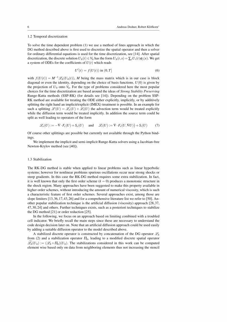
18 Andreas Dedner, Robert Klofkorn∗
(a) adaptation & no stabilization (b) adaptation & default stabilization
(c) adapted grid of a) (d) adapted grid of b)
Fig. 4: Top view of three body advection problem at time t = π using an adaptive grid.Left without stabilization and right with stabilization. Top shows solution with values above1+10−3 or below−10−3 are colored in grey and black, respectively. Bottom row shows cor-responding grid with solution colored according to their respective minimum and maximumvalues.
return conditional ( rho>1e-8, conditional ( p>1e-8 , 1, 0 ), 0 )
# for the residual indicator using the entropy equationclass Indicator :
def eta(t,x,U):_,_, p = Model. toPrim (U)return U[0]*ln(p/U[0]**Model.gamma)
def F(t,x,U,DU):s = Model. Indicator .eta(t,x,U)_,v,_ = Model. toPrim (U)return v*s
def S(t,x,U,DU):return 0
The next step is to fix the initial conditions and the end time for the two problems we wantto study. First for the shock bubble problem
Adding initial conditions for shock bubble problem to model class# shockgam = 1.4pinf , rinf = 5, ( 1-gam + (gam+1)*pinf )/( (gam+1) + (gam-1)*pinf )vinf = (1.0/sqrt(gam)) * (pinf - 1.)/ sqrt( 0.5*(( gam+1)/gam) * pinf +
0.5*(gam-1)/gam);Ul = Model. toCons ( [rinf ,vinf]+(dim-1)*[0]+[pinf] )Ur = Model. toCons ( [1]+dim*[0]+[1] )

Python Framework for Solving Evolution Equations with Stabilized DG 19
# bubblecenter , R2 = 0.5, 0.2**2bubble = Model. toCons ( [0.1]+dim*[0]+[1] )Model.U0 = conditional ( x[0]<-0.25 , Ul , conditional ( dot(x,x)<R2 , bubble , Ur) )Model. endTime = 0.5
To complete the description of the problem we need to define boundary conditions. For theadvection problem we used Dirichlet boundary conditions which are used as second statefor the numerical flux over the boundary segments. For this problem we will use Dirichletboundary conditions on the left and right boundary but want to use no flow boundary condi-tions on the top and bottom boundary (which will have an identifier of 3 on this domain):
Adding boundary conditions for shock bubble problem to Model classdef noFlowFlux (u,n):
_, _, p = Model. toPrim (u)return as_vector ([0]+[p*c for c in n]+[0])
Model. boundary = 1: lambda t,x,u: Ul ,2: lambda t,x,u: Ur ,3: lambda t,x,u,n: noFlowFlux (u,n)
Model. domain = ( reader .dgf , " shockbubble "+str(dim)+"d.dgf")
Next we describe initial conditions and boundary conditions for the Kelvin-Helmholtz insta-bility between two layers with a density jump where we use periodic boundary conditionsin the horizontal direction and reflective boundary conditions on the vertical boundaries:
Initial and boundary conditions for Kelvin-Helmholtz problemsigma = 0.05/sqrt(2)rho ,pres = conditional ( abs(x[1]-0.5)<0.25 ,2,1), 2.5u = conditional ( abs(x[1]-0.5)<0.25 ,0.5,-0.5)v = 0.1*sin(4*pi*x[0])*( exp(-(x[1]-0.25)**2/(2*sigma**2)) )Model.U0 = Model. toCons ([rho ,u,v,pres])def reflect (U,n):
n,m = as_vector (n), as_vector ([U[1],U[2]])mref = m - 2*dot(m,n)*nreturn as_vector ([U[0],*mref ,U[3]])
Model. boundary = 3: lambda t,x,U: reflect (U,[0,-1]),4: lambda t,x,U: reflect (U,[0,1])
Model. domain = ( reader .dgf , "kh.dgf")Model. endTime = 1.5
Now that we have set up the model class, the code presented for the advection problem forevolving the system and adapting the grid can remain unchanged.
Results for both test cases on locally adapted grids are shown in Fig. 5 and the middlecolumn of Fig. 6. The default setting works very well for the shock bubble interaction prob-lem. It turns out that in the Kelvin-Helmholtz case the stabilization is almost completelydetermined by the physicality check since the smoothness indicator shown here is based onthe pressure which in this case is continuous over the discontinuity. To increase the stabiliza-tion of the method it is either possible to reduce the tolerance in the troubled cell indicator orto use a different smoothness indicator all together, which is discussed in Section 2.4. Usingthe default setting for the indicator, very fine structures appear with considerable under- andovershoots developing as shown in the middle figure of Fig. 6. The minimum and maximumdensity are around 0.6 and 2.6, respectively. After increasing the sensitivity of the smooth-ness indicator, by passing a suitable parameter to the constructor of the operator to reducethe tolerance (using TOL = 0.2 here) the under- and overshoots are reduced to 0.8 and 2.4and some of the fine structure has been removed as shown on the right of Fig. 6. On the leftof the same figure we show results form a simulation using the indicator from [37] basedon the modal expansion of the density. Here minimum and maximum densities are 0.95 and2.1, respectively. More details of this indicator are provided in Section 2.4. As reference for
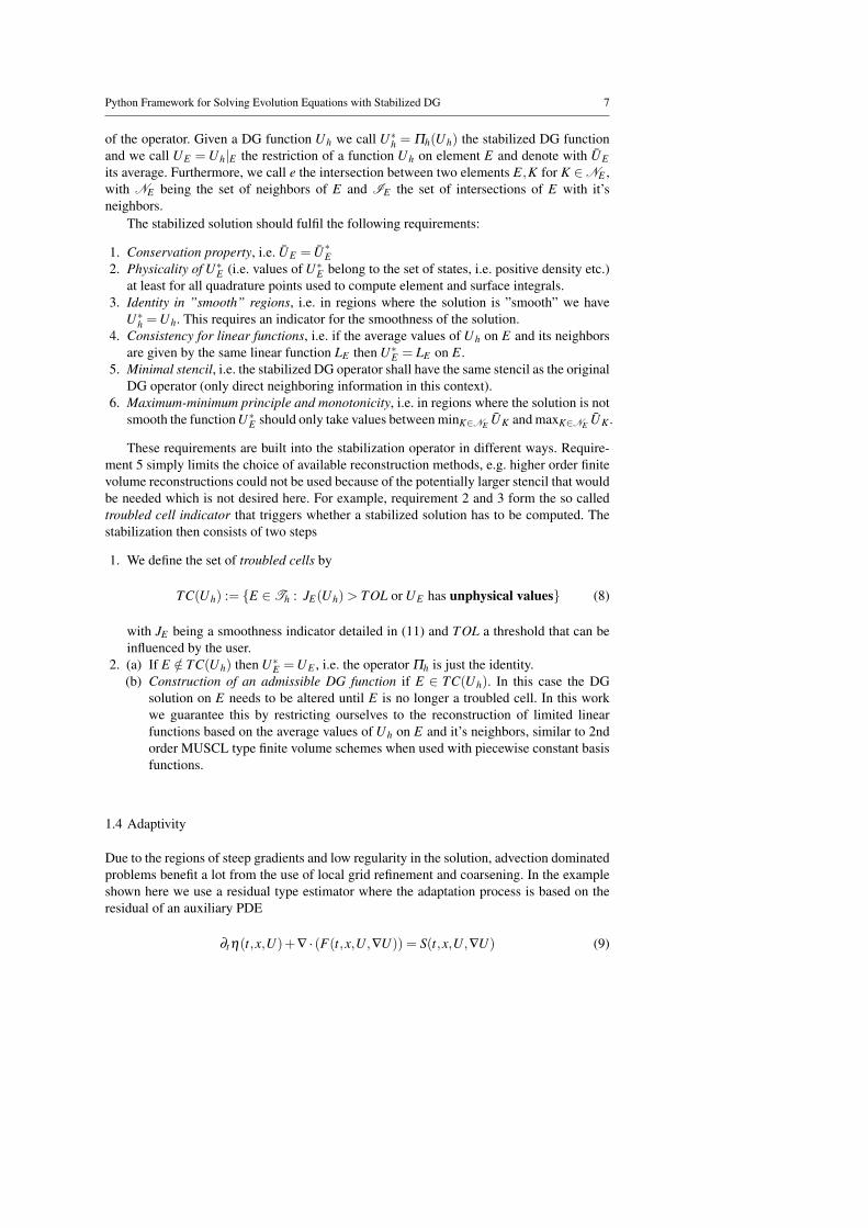
20 Andreas Dedner, Robert Klofkorn∗
Fig. 5: Shock bubble (actually column) interaction problem at t = 0.1 (left) and t = 0.5(right). Top figure shows the density and bottom figure the levels of the dynamically adaptedgrid.
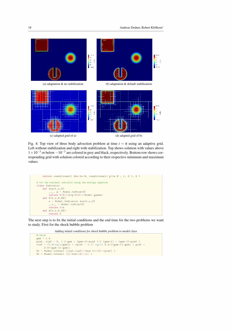
Fig. 6: Density (top) and grid levels (bottom) for Kelvin-Helmholtz instability at time t =1.5. In the initial setup the density in the upper layer is 2 and 1 in the lower layer. Themiddle figure shows the default setting for the troubled cell indicator which uses a toleranceof 1. The right figure shows results using a reduced tolerance of 0.2 so that more cellsare marked. On the left we show results obtained using the indicator from [37] based onthe modal expansion of the density. Details on how this indicator is added to the code isdiscussed in Section 2.4.
the Navier-Stokes simulation shown on the right of Fig. 8 density throughout the simulationwas in the range 0.97 and 2.1. This is discussed further in Section 2.4
2.3.2 Adding source terms
So far we have in fact simulated the interaction of a shock wave with a column of low densitygas and not in fact a bubble. To do the later would require to either extend the problem to3D (discussed in the next section) or to simulate the problem using cylindrical coordinates.This requires adding a geometric source term to the right hand side of the Euler equations.As pointed out in the introduction our model can take two types of source term depending

Python Framework for Solving Evolution Equations with Stabilized DG 21
Fig. 7: Shock bubble interaction problem in cylindrical coordinate at time t = 0.1 and t = 0.5.Density is shown in the top row and the adaptive grid in the bottom row.
upon the desired treatment in the time stepping scheme. Here we want to treat the sourceexplicitly so need to add an S_e method to the Model class:
Adding source term to Model class for Euler equations# geometric source term for cylindrical coordinatesdef source (t,x,U,DU):
_, v, p = Model. toPrim (U)return as_vector ([ - U[0] *v[1]/x[1],
- U[1] *v[1]/x[1], - U[2] *v[1]/x[1],-(U[3]+p)*v[1]/x[1] ])
Model.S_e = source# additional source term for residual indicatordef indicatorSource (t,x,U,DU):
s = Model. Indicator .eta(t,x,U)return - s * U[1]/U[0]/x[1]
Model. Indicator .S = indicatorSource
Results are shown in Fig. 7 which show a clear difference in the structure of the bubble atlater time compared to Fig. 5 which is matched by the structure of the full 3d simulationshown in Fig. 9.
2.3.3 Adding diffusion
Finally, we discuss the steps needed to add a diffusion term. This requires adding an ad-ditional method to the Model class. So to solve the compressible Navier-Stokes equationsinstead of the Euler equations the following method needs to be added (given a viscosityparameter µ):
Implementing Navier-Stokes by adding diffusion to Model class for Euler equationsdef F_v(t,x, U, DU):
assert dim == 2Pr = 0.72
rho , rhou , rhoE = U[0], as_vector ([U[j] for j in range(1,dim+1)]), U[dim+1]grad_rho = DU[0, :]grad_rhou = as_matrix ([[DU[j,:] for j in range (1, dim+1)]])[0]grad_rhoE = DU[dim+1,:]
grad_u = as_matrix ([[( grad_rhou [j,:]*rho - rhou[j]* grad_rho )/rho**2 for j inrange (dim)]])[0]
grad_E = ( grad_rhoE *rho - rhoE* grad_rho )/rho**2
tau = mu*( grad_u + grad_u .T - 2.0/3.0*tr( grad_u )* Identity (dim))K_grad_T = mu*Model.gamma/Pr*( grad_E - dot(rhou , grad_u )/rho)return as_matrix ([
[0.0, 0.0],[tau[0,0], tau[0,1]],[tau[1,0], tau[1,1]],

22 Andreas Dedner, Robert Klofkorn∗
Fig. 8: Diffusive Kelvin-Helmholtz instability with µ = 0 (Euler), µ = 0.0001, and µ =0.001 (from left to right). Top row shows density and bottom row the grid levels of theadaptive simulation. The smoothing effect of the viscosity is clearly visible compared tothe results shown for the Euler equations. Consequently, the small scale instabilities arecompletely suppressed and a coarser grid is used.
[dot(tau[0,:], rhou)/rho + K_grad_T [0], dot(tau[1,:], rhou)/rho +K_grad_T [1]] ])
As an example we repeat the simulation of the Kelvin-Helmholtz instability (see Fig. 8).Note that with the default setting for the stepper, an IMEX scheme is used where the dif-fusion is treated implicitly and the advection explicitly with a time step given by the CFLcondition. Consequently, we do not need to make any change to the construction of thespatial operator and time stepper shown in the code listing on Page 11.
2.4 User defined smoothness indicator
To exchange the smoothness indicator the construction of the operator has to be slightlychanged. Assuming that the indicator is defined in a source file modalindicator.hh whichdefines a C++ class ModalIndicator which takes the C++ type of the discrete function U_has template argument. This class needs to be derived from a pure virtual base class andoverride a single method. Then the construction of the operator needs to be changes to
Changing the smoothness indicator for the stabilization in the spatial operatorfrom dune. typeregistry import generateTypeNamefrom dune.femdg import smoothnessIndicator
# compile and load the module for the smoothness indicator - need the correct C++ typeclsName , includes = generateTypeName (" ModalIndicator ", U_h)# the ModelIndicator class has a default constructor (ctor) without argumentsindicator = smoothnessIndicator (clsName , [" modalindicator .hh"]+includes , U_h ,
ctorArgs =[])# construct the operatoroperator = femDGOperator (Model , space , limiter =[" default ",indicator ])
As an example we use here a smoothness indicator based on studying the decay proper-ties of the modal expansion of the solution on each cell following the ideas presented in[37]. For the following implementation we assume that we are using a modal basis functionset orthonormalized over the reference element. Then the C++ code required to computethe smoothness indicator based on the modal expansion of the density is given in the nextsnippets.

Python Framework for Solving Evolution Equations with Stabilized DG 23
template <class DiscreteFunction >struct ModalIndicator: public Dune::Fem:: TroubledCellIndicatorBase < DiscreteFunction >
using LocalFunctionType = DiscreteFunction :: LocalFunctionType ;ModalIndicator () double operator ()( const DiscreteFunction & U,
const LocalFunctionType & uEn) const override double modalInd = smoothnessIndicator ( uEn );return std::abs( modalInd ) > 1e-14? 1. / modalInd : 0.;
The actual computation of the indicator is carried out in the method smoothnessIndicatorbut is slightly too long to include here directly but is shown in Appendix C. It is important tonote that it requires very little knowledge of the DUNE programming environment or evenC++ since it relies mainly on the local degrees of freedom vector provided by the argumentuEn. Simulation results for the Kelvin-Helmholtz instability using this indicator are includedin Fig. 6.
2.5 User defined time stepping schemes
The DUNE-FEM package provides a number of standard strong stability preserving Runge-Kutta (SSP RK) solvers including explicit, diagonally implicit, and IMEX schemes of de-gree one to four. In the literature there is a wide range of additional suitable RK methods(having low storage or better CFL constants using additional stages for example). Further-more, multistep methods can be used. Also there are a number of other packages providingimplementations of timestepping methods. Since the computationally critical part of a DGmethod of the type described here lies in the computation of the spatial operator, the ad-ditional work needed for the timestepper can be carried out on the Python side with littleimpact. Furthermore, as pointed out in the introduction, it is often desirable to use Pythonfor rapid prototyping and to then reimplement the finished algorithm in C++ after a firsttesting phase to avoid even the slightest impact on performance. The following code snippetshows how a multistage third order RK method taken from [35] can be easily implementedin Python and used to replace the stepper used so far:
Implementation of time stepping method on Python sideclass ExplSSP3 :
def __init__ (self ,stages ,op ,cfl=0.45):self.op = opself.n = int(sqrt( stages ))self. stages = self.n*self.nself.r = self. stages -self.nself.q2 = op.space. interpolate (op.space. dimRange *[0],name="q2")self.tmp = self.q2.copy ()self.cfl = cfl * stages *(1-1/self.n)self.dt = None
def c(self ,i):return (i-1)/(self.n*self.n-self.n) \
if i<=(self.n+2)*(self.n-1)/2+1 \else (i-self.n-1)/(self.n*self.n-self.n)
def __call__ (self ,u,dt=None):if dt is None and self.dt is None:
self.op. stepTime (0,0)self.op(u, self.tmp)dt = self.op. timeStepEstimate [0]*self.cfl
elif dt is None:dt = self.dt
self.dt = 1e10

24 Andreas Dedner, Robert Klofkorn∗
Fig. 9: Adaptive 3D simulation of shock bubble interaction problem shown from two dif-ferent sides. The grid levels and the density distribution at time t = 0.5 is shown togetherwith the isosurface ρ = 1.5. The simulation was performed on a workstation using 8 proces-sors. The corresponding globally refined grid would have contained 1.5M elements resultingin 52M degrees of freedom. The grid shown here consists of 150.000 elements with about5.2M degrees of freedom.
fac = dt/self.ri = 1while i <= (self.n-1)*(self.n-2)/2:
self.op. stepTime (self.c(i),dt)self.op(u,self.tmp)self.dt = min(self.dt , self.op. timeStepEstimate [0]*self.cfl)u.axpy(fac , self.tmp)i += 1
self.q2. assign (u)while i <= self.n*(self.n+1)/2:
self.op. stepTime (self.c(i),dt)self.op(u,self.tmp)self.dt = min(self.dt , self.op. timeStepEstimate [0]*self.cfl)u.axpy(fac , self.tmp)i += 1
u. as_numpy [:] *= (self.n-1)/(2*self.n-1)u.axpy(self.n/(2*self.n-1), self.q2)while i <= self. stages :
self.op. stepTime (self.c(i),dt)self.op(u,self.tmp)self.dt = min(self.dt , self.op. timeStepEstimate [0]*self.cfl)u.axpy(fac , self.tmp)i += 1
self.op. applyLimiter ( u )self.op. stepTime (0,0)return dt
# use a four stage version of this stepperstepper = ExplSSP3 (4, operator )
Again the other parts of the code can remain unchanged. Results with this time steppingscheme are included in some of the comparisons shown in the next section (see Fig. 11 andFig. 12).
2.6 Different grids and spaces
One of the strengths of the DUNE framework on which we are basing the software presentedhere, is that it can handle many different types of grid structures. Performing a 3D simulationcan be as simple as changing the domain attribute in the Model class (Fig. 9).

Python Framework for Solving Evolution Equations with Stabilized DG 25
Fig. 10: Shock bubble interaction problem at t = 0.1 using different grid structures. A struc-tured simplex grid (left), a non affine cube grid (right), a polygonal grid (middle) consistingof the dual of the simplex grid on the left.
It is also straightforward to perform the simulations on for example a simplicial gridinstead of the cube grid used so far:
Changing the grid structure (simplex grid)from dune. alugrid import aluSimplexGrid as grid
gridView = view( grid( Model. domain ) )gridView . hierarchicalGrid . globalRefine (3) # refine a possibly coarse initial grid
It is even possible to use a grid consisting of general polygonal elements, by simply import-ing the correct grid implementation:
Changing the grid structure (polyhedral grid)from dune. polygongrid import polygonGrid as grid
A wide range of other grid types are available and a recent overview is given in [6] someexamples are shown in Fig. 10.
As pointed out in the previous section, the choice of the basis function set used to rep-resent the discrete solution can strongly influence the efficiency of the simulation. So farwe have used an orthonormal basis function set for the polynomial space over the referencecube [0,1]d . If the grid elements are all affine mapping of [0,1]d (i.e. parallelograms) thenthis is good choice, since it has the minimal number of degrees of freedom for a desiredapproximation accuracy while the mass matrix will be a very simple diagonal matrix onall elements. These properties always hold for simplicial elements when an orthonormalpolynomial basis over the reference simplex is used. As soon as the mapping between thereference element and a given element in the grid becomes non affine, both properties canbe lost. To achieve the right approximation properties in this case, it might be necessary,to use a tensor product polynomial space, increasing the number of degrees of freedom perelement considerably. Also an orthonormal set of basis function over the reference cube,will still lead to a dense mass matrix. This lead to a significant reduction in the efficiencyof the method, if the local mass matrix on each element can not be stored due to memoryrestrictions. A possible solution to this problem is to use a Lagrange type set of basis func-tions with interpolation points coinciding with a quadrature rule over the reference cube.We discussed this approach in some detail in Section 1.1. There we mentioned two choices
26 Andreas Dedner, Robert Klofkorn∗
for such quadrautre: the use of tensor product Gauss-Legendre rules which are optimal withrespect to accuracy. In the software framework presented here, it is straightforward to switchto this representation of the discrete space by replacing the construction of the space objectby
Changing the discrete space (dg space using Lagrange type basis functions)from dune.fem.space import dglagrangespace = dglagrange ( gridView , dimRange =Model.dimRange , order=4, pointType ="gauss" )
If the operator is constructed using this space, the suitable Gaussian quadrature is chosenautomatically. Note that this space is only well defined over a grid consisting of cubes. Asecond common choice, which corresponds to an underintegration of the mass matrix butfaster evaluation of surface integrals, is to use Lobatto-Gauss-Legendre (LGL) quadraturerules. Again switching to this Lagrange point set is straightforward
Changing the discrete space (dg space using spectral basis functions)space = dglagrange (gridView , dimRange =Model.dimRange , order=4, pointType =" lobatto ")
and again using this space in the construction of the spatial operator will result in the correctLGL quadrature being used.
In Fig. 11, 12 we compare L2 errors on a sequence of non affine cube grids (split into 2simplices for the simplicial simulation) using different sets of basis functions. We show boththe error in the L2 vs. the number of degrees of freedom (left) and vs. the runtime (right).The right plot also includes results from a simulation with the LGL method and the SSP3time stepper implemented in Python as discussed previously. The results of this simulationare not included on the left since they are broadly in line with the LGL simulation using the3 stage RK method available in DUNE-FEM-DG.
Summarizing the results from both Fig. 11, 12 it seems clear that the simulation on thesimplicial grid produces a slightly better error on the same grid but requires twice as manydegrees of freedom so that it is less efficient compared to the LGL or GL simulations. Alsoas expected, the runtime with the ONB basis on the cube grids is significantly larger dueto the additional cost of computing the inverse mass matrix on each element of the grid asdiscussed above. On an affine cube grid the runtime is comparable to the GL scheme on thesame grid but this is not shown here. Finally, due to the larger effective CFL constant thetime stepper implemented in Python is more efficient then the 3 stage method of the sameorder available in DUNE-FEM-DG.
In Fig. 13 we carry out the same experiment but this time using the orthonormal basis butvarying the troubled cell indicator. While all method seem to broadly converge in a similarfashion when the grids are refined, it is clear that the main difference in the efficiency isagain based on question if the grid elements are affine mappings of the reference element ornot. For a given grid structure the results indicate that using the modal indicator based onthe density is the most efficient for the given test case.
2.7 Reactive advection diffusion problem
We conclude with an example demonstrating the flexibility of the framework to combinedifferent components of the DUNE-FEM package to construct a scheme for a more complexproblem. As a simple example we use a chemical reaction type problem with linear advec-tion and diffusion where the velocity field is given by discretizing the solution to an ellipticproblem in a continuous Lagrange space. As mentioned this is still a simple problem but can

Python Framework for Solving Evolution Equations with Stabilized DG 27
0.001
0.01
0.1
1000 10000 100000
L2 e
rro
r
number of degrees of freedom
non affine GLnon affine LGLnon affine ONB
simplex
0.001
0.01
0.1
0.1 1 10 100 1000
L2 e
rro
r
total runtime
non affine GLnon affine LGLnon affine ONB
simplexnon affine LGL with 4stage RK
Fig. 11: Two rarefaction wave problem simulated from t = 0.05 to 0.12 on a sequence ofnon-affine cube and on simplicial grids with different representation for the discrete spacewith polynomial order 4.
0.01
100000 1x10⁶
L2 e
rro
r
number of degrees of freedom
non affine GLnon affine LGLnon affine ONB
simplex
0.01
10 100 1000 10000
L2 e
rro
r
total runtime
non affine GLnon affine LGLnon affine ONB
simplexnon affine LGL with 4stage RK
Fig. 12: Sod’s Riemann problem simulated from t = 0 to 0.2 on a sequence of non-affinecube and on simplicial grids with different representation for the discrete space with poly-nomial order 4.
0.01
100000 1x10⁶
L2 e
rro
r
number of degrees of freedom
none affine cube, jumpsimplex, jump
none affine cube, modal densitysimplex, modal density
none affine cube, modal pressuresimplex, modal pressure
0.01
100 1000 10000
L2 e
rro
r
total runtime
non affine cube, jumpsimplex, jump
non affine cube, modal densitysimplex, modal density
none affine cube, modal pressuresimplex, modal pressure
Fig. 13: Sod’s Riemann problem simulated from t = 0 to 0.2 using different troubled cellindicators. The simulations were performed on a sequence of grids consisting of non affinecubes (split into two triangles for simplicial simulations) using piecewise polynomials oforder 4 with the orthonormal basis. Shown are the errors measured in the L2 norm versusthe number of degrees of freedom (left) and the runtime (right).

28 Andreas Dedner, Robert Klofkorn∗
be seen as a template for coupled problems, e.g., transport in porous media setting or wherethe flow is given by solving incompressible Navier Stokes equations.
Let us first compute the velocity given as the curl of the solution to a scalar ellipticproblem:
Computing a velocity field given as curl of solution to Laplace problemstreamSpace = lagrange (gridView , order=order)Psi = streamSpace . interpolate (0,name=" streamFunction ")u,v = TrialFunction ( streamSpace ), TestFunction ( streamSpace )x = SpatialCoordinate ( streamSpace )form = ( inner(grad(u),grad(v)) - 5*sin(x[0])*sin(x[1]) * v ) * dxstreamScheme = galerkin ([form == 0, DirichletBC ( streamSpace ,0) ])streamScheme .solve( target =Psi)transportVelocity = as_vector ([-Psi.dx(1),Psi.dx(0)])
We use this velocity field to evolve three chemical components reacting through some non-linear reaction term and include some small linear diffusion:
Model class for chemical reaction problemfrom ufl import *from dune.ufl import DirichletBCfrom dune.fem.space import lagrangefrom dune.fem. scheme import galerkin
class Model:dimRange = 3# source term (treated explicitly)def S_e(t,x,U,DU):
# reaction termr = 10* as_vector ([U[0]*U[1], U[0]*U[1], -2*U[0]*U[1]])# source for component one and twoP1 = as_vector ([0.2*pi ,0.2*pi]) # midpoint of first sourceP2 = as_vector ([1.8*pi ,1.8*pi]) # midpoint of second sourcef1 = conditional (dot(x-P1 ,x-P1) < 0.2, 1, 0)f2 = conditional (dot(x-P2 ,x-P2) < 0.2, 1, 0)f = conditional (t<5, as_vector ([f1 ,f2 ,0]), as_vector ([0,0,0]))return f - r
# diffusion termdef F_v(t,x,U,DU):
return 0.02*DU# advection termdef F_c(t,x,U):
return as_matrix ([ [*(Model. velocity (t,x,U)*u)] for u in U ])def maxWaveSpeed (t,x,U,n):
return abs(dot(Model. velocity (t,x,U),n))# dirichlet boundary conditionsboundary = range (1,5): as_vector ([0,0,0])# initial conditionsU0 = [0,0,0]endTime = 10
Note that the source term includes both the chemical reaction and a source for the first twocomponents. The third component is generated by the first two interacting.
Due to the diffusion we do not need any stabilization of the form used so far. However,in this case a reasonable assumption is that all components remain positive throughout thesimulation, so the physicality check described above is still a useful feature. We can combinethis with the scaling limiter already described for the advection problem. To this end we needto add bounds to the model and change to the construction call for the operator:
Using scaling limiterModel. lowerBound = [0,0,0]operator = femDGOperator (Model , space , limiter =" scaling ")
Note that by default the stepper switches to a IMEX Runge-Kutta scheme if the Model classcontains both an advective and a diffusive flux. This behavior can be changed by using the

Python Framework for Solving Evolution Equations with Stabilized DG 29
Fig. 14: The three components of the chemical reaction system (left to right) at t = 4.5 (toprow) and t = 10 (bottom row). Velocity field included in middle figure.
rkType parameter in the constructor call for the stepper. A final remark concerning bound-ary conditions: here we use simple Dirichlet boundary conditions which are then used forboth the diffusive and advective fluxes on the boundary as outside cell value. We saw in aprevious example that we can also prescribe the advective flux on the boundary directly. Inthat example we used
Boundary conditionsModel. boundary [3] = lambda t,x,u,n: noFlowFlux (u,n)
If this type of boundary conditions is used we also need to prescribe the flux for the diffusionterm, so for an advection-diffusion problem we pass in a pair of fluxes at the boundary, e.g.,
Flux boundary conditions for advection-diffusion problemModel. boundary [3] = [ lambda t,x,U,n: inner( Model.Fc(t,x,Ubnd), n ),
lambda t,x,U,DU ,n: inner( Model.Fv(t,x,Ubnd ,DUbnd), n ) ]
Fig. 14 shows the results for the chemical reaction problem.
3 Efficiency of Python based auto-generated models
While Python is easy to use, its flexibility can lead to some deficiencies when it comes toperformance. In DUNE [23,16] a just-in-time compilation concept is used to create Pythonmodules based on the static C++ type of every object used, i.e. the models described inthe previous section are translated into C++ code based on the UFL descriptions in thevarious model methods which is then compiled and loaded as Python modules. This way weavoid virtualization of the DUNE interfaces and consequently one would expect very littleperformance impact as long as calls between Python and C++ are only done for long runningmethods. To verify this, we compare the performance of the approach shown here with thepreviously hand-coded pure C++ version described in [14].
As a test example we choose a standard Riemann problem (Sod, T = 0.1) for the Eulerequations solved on a series of different grid resolutions using forth order basis functions,

30 Andreas Dedner, Robert Klofkorn∗
Table 1: Runtime comparison of the C++ and the Python code for a simple test examplesolving the Euler equations in 2d with explicit time stepping and forth order polynomialsusing 1 and 4 thread(s).
4th order polynomials and 1 thread.SPGrid
code\ #el 1024 4096 16384
C++ 15.5 128.6 1045.4C++(UFL) 14.8 123.7 1013.2Python 14.8 123.9 1008.6
ALUGridcode\ #el 1024 4096 16384
C++ 17.3 145.6 1203.5C++(UFL) 17. 3 145.0 1199.3Python 19.5 163.3 1341.7
4th order polynomials and 4 threads.SPGrid
code\ #el 1024 4096 16384
C++ 4.43 35.7 291.2C++(UFL) 4.18 34.4 282.0Python 4.19 34.1 280.9
ALUGridcode\ #el 1024 4096 16384
C++ 4.79 39.9 331.3C++(UFL) 4.73 39.9 331.5Python 5.43 44.2 365.7
the default limiter, and explicit RK3 time stepping with CFL = 0.4. We use two differ-ent grid implementation, a dedicated Cartesian grid (SPGrid) and a fully unstructured grid(ALUGrid). The results are shown in Table 1 and should be taken with a grain of salt sincethese only present a preliminary comparison, as such measurements heavily depend on thehardware, compiler and compiler flags as well as selected mathematical problem. The re-sults presented here were produced on an Intel CPU i7-9750H @ 2.60GHz using g++-9.3and the following compiler flags:
-O3 - DNDEBUG - Wfatal - errors -march= native -fomit-frame- pointer -ftree- vectorize- fexpensive - optimizations --param large-unit-insns=500--param inline -unit- growth =500 --param max- inline -insns- single =500--param large- function - growth =500 --param large- function -insns=500
With our setting we observe that for the Cartesian grid (SPGrid) using the Python front-end leads to no performance loss. For the unstructured grid (ALUGrid) we observe a perfor-mance decrease of about 10%. This can be explained with the fact that for SPGrid all codecan be inlined in the just-in-time compiled Python module which uses the same compileroptimization flags as the normal C++ code. For ALUGrid, where a shared library exists, thisis not so straight forward. In the future we will experiment with link time optimization andtry to reduce implementation of small code snippets in the ALUGrid library.
4 Conclusion and outlook
In this paper we presented a comprehensive framework for the Discontinuous Galerkin (DG)method with an easy to use Python interface for model description and solver configuration.The framework covers different variants of existing DG methods and can be easily extendedto include improvements and new development of the methodology.
Although the DUNE-FEM-DG framework serves as a good starting point for high-performance DG solvers, the aim of this work is to demonstrate how the Python interfacesimplifies the simulation of a wide range of evolution equations as well as enabling the rapidprototyping of new methods, their testing and their comparison with other methods. For ex-ample, in almost all the tests presented here, computations were done using the same setting

Python Framework for Solving Evolution Equations with Stabilized DG 31
for the indicator and tolerance for adaptivity and the troubled cell detection, demonstratingthe robustness of the default setup. Of course the default setup will only be a suitable start-ing point and so most of the building blocks of the discretization can be straightforwardlyreplaced from within the Python script, often without requiring any or not much C++ knowl-edge. Also we would like to point out the implemented DG solver can be directly used ashigher (2nd) order Finite Volume (FV) scheme by replacing the DG space with a FV spaceconsisting of piecewise constant polynomials.
The Python interfaces are not yet fully reflecting the possibilities on the C++ side, forexample, the reconstruction in primary variables for the Euler equations is possible, but notyet available on the Python side. Another missing feature is that it is currently not possible onthe Python side to easily exchange the average operators in the discretization of the diffusiveterms as, for example, needed in some applications [15].
Another missing feature in Python is the assembly of Jacobian matrices during thenonlinear solve. This could be desirable for some applications or to test different existingsolvers. Although the feature is available in the C++ code it needs a few code alterations inthe underlying infrastructure package. This would also make it straightforward to then useother solver packages available in Python, e.g., scipy. For the compressible applications,which were the focus of this work, it is much more feasible to work with the Jacobian freenonlinear solvers and there robust and efficient preconditioning techniques are still a veryactive research topic. We are currently focusing on including ideas presented in [7] based onsubcell finite volume multigrid preconditioning.
The extension of the DGSEM methods to simplicial grids (see [11] for an overview)could be implemented with a few minor modifications. Based on earlier work [22] the nec-essary basis function implementations for arbitrary quadrature points are available but needto be integrated into the DUNE-FEM and DUNE-FEM-DG framework.
While DUNE-FEM provides a number of Runge-Kutta methods, we have shown herethat it is straightforward to add other time stepping algorithms on the Python side, a featurewhich should also allow to use other packages which provide bindings for Python, suchas the Assimulo package [2]. For IMEX schemes the splitting is at the moment still a bitrestricted focusing on the important case of implicitly treating the diffusion (and part ofthe source term) while using an explicit method for the advection. In some applicationsother types of splitting (e.g. horizontal explicit vertical implicit (HEVI) methods used inmeteorology) are of interest and will be made available in future releases.
Conflict of interest
On behalf of all authors, the corresponding author states that there is no conflict of interest.
References
1. Alnæs, M.S., Logg, A., Ølgaard, K.B., Rognes, M.E., Wells, G.N.: Unified Form Language: A domain-specific language for weak formulations of partial differential equations. CoRR abs/1211.4047 (2012).URL http://arxiv.org/abs/1211.4047
2. Andersson, C., Fuhrer, C., Akesson, J.: Assimulo: A unified framework for ODE solvers. Mathematicsand Computers in Simulation 116(0), 26 – 43 (2015). doi:10.1016/j.matcom.2015.04.007
3. Balay, S., Abhyankar, S., Adams, M.F., Brown, J., Brune, P., Buschelman, K., Dalcin, L., Dener, A.,Eijkhout, V., Gropp, W.D., Karpeyev, D., Kaushik, D., Knepley, M.G., May, D.A., McInnes, L.C., Mills,R.T., Munson, T., Rupp, K., Sanan, P., Smith, B.F., Zampini, S., Zhang, H., Zhang, H.: PETSc usersmanual. Tech. Rep. ANL-95/11 - Revision 3.14, Argonne National Laboratory (2020). URL https://www.mcs.anl.gov/petsc

32 Andreas Dedner, Robert Klofkorn∗
4. Bangerth, W., Hartmann, R., Kanschat, G.: deal.II – a general purpose object oriented finite elementlibrary. ACM Trans. Math. Softw. 33(4), 24/1–24/27 (2007). URL http://dealii.org/
5. Bastian, P., Blatt, M., Dedner, A., Engwer, C., Klofkorn, R., Kornhuber, R., Ohlberger, M., Sander, O.:A Generic Grid Interface for Parallel and Adaptive Scientific Computing. Part II: Implementation andTests in DUNE. Computing 82(2–3), 121–138 (2008). doi:10.1007/s00607-008-0004-9
6. Bastian, P., Blatt, M., Dedner, M., Dreier, N.A., Engwer Ch. Fritze, R., Graser, C., Gruninger, C., Kempf,D., Klofkorn, R., Ohlberger, M., Sander, O.: The Dune framework: Basic concepts and recent develop-ments. CAMWA (2020). doi:10.1016/j.camwa.2020.06.007
7. Birken, P., Gassner, G.J., Versbach, L.M.: Subcell finite volume multigrid preconditioning for high-orderdiscontinuous galerkin methods. International Journal of Computational Fluid Dynamics 33(9), 353–361(2019). doi:10.1080/10618562.2019.1667983
8. Brdar, S., Baldauf, M., Dedner, A., Klofkorn, R.: Comparison of dynamical cores for NWP models:comparison of COSMO and DUNE. Theoretical and Computational Fluid Dynamics 27(3-4), 453–472(2013). doi:10.1007/s00162-012-0264-z
9. Brdar, S., Dedner, A., Klofkorn, R.: Compact and stable Discontinuous Galerkin methods for convection-diffusion problems. SIAM J. Sci. Comput. 34(1), 263–282 (2012). doi:10.1137/100817528
10. Chen, L., Li, R.: An Integrated Linear Reconstruction for Finite Volume scheme on Unstructured Grids.J. Sci. Comput. 68, 1172–1197 (2016). doi:10.1007/s10915-016-0173-1
11. Chen, T., Shu, C.W.: Review Article: Review of Entropy Stable Discontinuous Galerkin Methods forSystems of Conservation Laws on Unstructured Simplex Meshes. CSIAM Transactions on AppliedMathematics 1(1), 1–52 (2020). doi:10.4208/csiam-am.2020-0003
12. Cheng, Y., Li, F., Qiu, J., Xu, L.: Positivity-preserving DG and central DG methods for ideal MHDequations. Journal of Computational Physics 238, 255 – 280 (2013). doi:10.1016/j.jcp.2012.12.019
13. Cockburn, B., Shu, C.W.: Runge-Kutta Discontinuous Galerkin methods for convection-dominated prob-lems. J. Sci. Comput. 16(3), 173–261 (2001)
14. Dedner, A., Girke, S., Klofkorn, R., Malkmus, T.: The DUNE-FEM-DG module. ANS 5(1) (2017).doi:10.11588/ans.2017.1.28602
15. Dedner, A., Kane, B., Klofkorn, R., Nolte, M.: Python framework for hp-adaptive discontinu-ous Galerkin methods for two-phase flow in porous media. AMM 67, 179 – 200 (2019).doi:10.1016/j.apm.2018.10.013
16. Dedner, A., Kloefkorn, R., Nolte, M.: Python bindings for the dune-fem module (2020).doi:10.5281/zenodo.3706994
17. Dedner, A., Klofkorn, R.: A Generic Stabilization Approach for Higher Order DiscontinuousGalerkin Methods for Convection Dominated Problems. J. Sci. Comput. 47(3), 365–388 (2011).doi:10.1007/s10915-010-9448-0
18. Dedner, A., Klofkorn, R.: The Dune-Fem-DG Module. https://gitlab.dune-project.org/dune-fem/dune-fem-dg (2019)
19. Dedner, A., Klofkorn, R.: A Python Framework for Solving Advection-Diffusion Problems. In:R. Klofkorn, E. Keilegavlen, F.A. Radu, J. Fuhrmann (eds.) Finite Volumes for Complex ApplicationsIX - Methods, Theoretical Aspects, Examples, pp. 695–703. Springer International Publishing, Cham(2020). doi:10.1007%2F978-3-030-43651-3 66
20. Dedner, A., Klofkorn, R., Nolte, M., Ohlberger, M.: A Generic Interface for Parallel and Adaptive Sci-entific Computing: abstraction Principles and the DUNE-FEM Module. Computing 90(3–4), 165–196(2010). doi:10.1007/s00607-010-0110-3
21. Dedner, A., Makridakis, C., Ohlberger, M.: Error control for a class of Runge-Kutta discontinuousGalerkin methods for nonlinear conservation laws. SIAM J. Numer. Anal. 45(2), 514–538 (2007).doi:10.1137/050624248
22. Dedner, A., Nolte, M.: Construction of Local Finite Element Spaces Using the Generic Reference Ele-ments. In: A. Dedner, B. Flemisch, R. Klofkorn (eds.) Advances in DUNE, pp. 3–16. Springer BerlinHeidelberg, Berlin, Heidelberg (2012). doi:10.1007/978-3-642-28589-9 1
23. Dedner, A., Nolte, M.: The Dune-Python Module. CoRR abs/1807.05252 (2018). URL http://arxiv.org/abs/1807.05252
24. Discacciati, N., Hesthaven, J.S., Ray, D.: Controlling oscillations in high-order Discontinuous Galerkinschemes using artificial viscosity tuned by neural networks. Journal of Computational Physics 409,109304 (2020). doi:10.1016/j.jcp.2020.109304
25. Dolejsı, V., Feistauer, M., Schwab, C.: On some aspects of the discontinuous Galerkin finite elementmethod for conservation laws. Mathematics and Computers in Simulation 61(3), 333 – 346 (2003).doi:10.1016/S0378-4754(02)00087-3
26. Dumbser, M., Balsara, D.S., Toro, E.F., Munz, C.D.: A unified framework for the construction of one-stepfinite volume and discontinuous Galerkin schemes on unstructured meshes. Journal of ComputationalPhysics 227(18), 8209 – 8253 (2008). doi:10.1016/j.jcp.2008.05.025

Python Framework for Solving Evolution Equations with Stabilized DG 33
27. The Feel++ Consortium: The Feel++ Book (2015). URL https://www.gitbook.com/book/feelpp/feelpp-book
28. Feistauer, M., Kucera, V.: A new technique for the numerical solution of the compressible Euler equa-tions with arbitrary Mach numbers. Benzoni-Gavage, Sylvie (ed.) et al., Hyperbolic problems. Theory,numerics and applications. Proceedings of the 11th international conference on hyperbolic problems,Ecole Normale Superieure, Lyon, France, July 17–21, 2006. Berlin: Springer. 523-531 (2008). (2008)
29. Gottlieb, S., Shu, C.W., Tadmor, E.: Strong Stability-Preserving High-Order Time Discretization Meth-ods. SIAM Rev. 43(1), 89–112 (2001). doi:10.1137/S003614450036757X
30. Guermond, J.L., Pasquetti, R., Popov, B.: Entropy viscosity method for nonlinear conservation laws.Journal of Computational Physics 230(11), 4248 – 4267 (2011). doi:10.1016/j.jcp.2010.11.043. Specialissue High Order Methods for CFD Problems
31. Hindenlang, F., Gassner, G.J., Altmann, C., Beck, A., Staudenmaier, M., Munz, C.D.: Explicit dis-continuous Galerkin methods for unsteady problems. Computers & Fluids 61, 86 – 93 (2012).doi:10.1016/j.compfluid.2012.03.006
32. Honig, J., Koch, M., Rude, U., Engwer, C., Kostler, H.: Unified generation of DG-kernels for differentHPC frameworks. In: I. Foster, G.R. Joubert, L. Kucera, W.E. Nagel, F. Peters (eds.) Advances in ParallelComputing, vol. 36, pp. 376–386. IOS Press BV (2020). doi:10.3233/APC200062
33. Houston, P., Sime, N.: Automatic Symbolic Computation for Discontinuous Galerkin Finite ElementMethods. SIAM Journal on Scientific Computing 40(3), C327–C357 (2018). doi:10.1137/17M1129751
34. Karniadakis, G., Sherwin, S.: Spectral/hp element methods for computational fluid dynamics. OxfordUniversity Press (2005). URL http://www.nektar.info/
35. Ketcheson, D.I.: Highly Efficient Strong Stability-Preserving Runge-Kutta Methods with Low-Storage Implementations. SIAM Journal on Scientific Computing 30(4), 2113–2136 (2008).doi:10.1137/07070485X
36. Klieber, W., Riviere, B.: Adaptive simulations of two-phase flow by discontinuous Galerkin methods.Comput. Methods Appl. Mech. Eng. 196(1-3), 404–419 (2006). doi:10.1016/j.cma.2006.05.007
37. Klockner, A., Warburton, T., Hesthaven, J. S.: Viscous shock capturing in a time-explicit discontinuousgalerkin method. Math. Model. Nat. Phenom. 6(3), 57–83 (2011). doi:10.1051/mmnp/20116303
38. Klofkorn, R.: Efficient Matrix-Free Implementation of Discontinuous Galerkin Methods for Compress-ible Flow Problems. In: A.H. et al. (ed.) Proceedings of the ALGORITMY 2012, pp. 11–21 (2012)
39. Klofkorn, R., Kvashchuk, A., Nolte, M.: Comparison of linear reconstructions for second-order fi-nite volume schemes on polyhedral grids. Computational Geosciences 21(5), 909–919 (2017).doi:10.1007/s10596-017-9658-8
40. Knoll, D.A., Keyes, D.E.: Jacobian-free Newton-Krylov methods: a survey of approaches and applica-tions. J. Comput. Phys. 193(2), 357–397 (2004)
41. Kopriva, D.A., Gassner, G.: On the quadrature and weak form choices in collocation type discon-tinuous galerkin spectral element methods. Journal of Scientific Computing 44, 136–155 (2010).doi:10.1007/s10915-010-9372-3
42. Kopriva, D.A., Woodruff, S.L., Hussaini, M.Y.: Computation of electromagnetic scattering with a non-conforming discontinuous spectral element method. International Journal for Numerical Methods inEngineering 53(1), 105–122 (2002). doi:10.1002/nme.394
43. Krivodonova, L., Xin, J., Remacle, J.F., Chevaugeon, N., Flaherty, J.E.: Shock detection and limitingwith discontinuous Galerkin methods for hyperbolic conservation laws. Appl. Numer. Math. 48(3-4),323–338 (2004). doi:10.1016/j.apnum.2003.11.002
44. Logg, A., Mardal, K.A., Wells, G.: Automated Solution of Differential Equations by the Finite ElementMethod: The FEniCS Book. Springer Publishing Company, Incorporated (2012)
45. Mandli, K.T., Ahmadia, A.J., Berger, M., Calhoun, D., George, D.L., Hadjimichael, Y., Ketcheson, D.I.,Lemoine, G.I., LeVeque, R.J.: Clawpack: building an open source ecosystem for solving hyperbolic pdes.PeerJ Computer Science 2, e68 (2016). doi:10.7717/peerj-cs.68
46. May, S., Berger, M.: Two-dimensional slope limiters for finite volume schemes on non-coordinate-aligned meshes. SIAM Journal on Scientific Computing 35(5), A2163–A2187 (2013).doi:10.1137/120875624
47. Persson, P.O., Peraire, J.: Sub-cell shock capturing for discontinuous galerkin methods. presented at 44thaiaa aerospace sciences meeting, aiaa-2006-0112, reno, nevada, Department of Aeronautics & Astronau-tics Massachusetts Institute of Technology (2006). doi:10.2514/6.2006-112
48. Rathgeber, F., Ham, D.A., Mitchell, L., Lange, M., Luporini, F., McRae, A.T.T., Bercea, G.T., Markall,G.R., Kelly, P.H.J.: Firedrake: Automating the Finite Element Method by Composing Abstractions. ACMTrans. Math. Softw. 43(3), 24:1–24:27 (2016). doi:10.1145/2998441
49. Schuster, D., Brdar, S., Baldauf, M., Dedner, A., Klofkorn, R., Kroner, D.: On discontinuous Galerkinapproach for atmospheric flow in the mesoscale with and without moisture. Meteorologische Zeitschrift23(4), 449–464 (2014). doi:10.1127/0941-2948/2014/0565
34 Andreas Dedner, Robert Klofkorn∗
50. Shu, C.W.: High order WENO and DG methods for time-dependent convection-dominated PDEs: Abrief survey of several recent developments. Journal of Computational Physics 316, 598 – 613 (2016).doi:10.1016/j.jcp.2016.04.030
51. Wallwork, J.G., Barral, N., Kramer, S.C., Ham, D.A., Piggott, M.D.: Goal-oriented error estimation andmesh adaptation for shallow water modelling. SN Applied Sciences 2 (2020). doi:10.1007/s42452-020-2745-9
52. Zhang, X., Shu, C.W.: On positivity-preserving high order discontinuous Galerkin schemes for com-pressible Euler equations on rectangular meshes. Journal of Computational Physics 229(23), 8918 –8934 (2010). doi:10.1016/j.jcp.2010.08.016
A Installation
The presented software is based on the upcoming DUNE release version 2.8. Installing the software describedin this paper can be done using the Package Installer for Python (pip). This method of installing the softwarehas been tested on different Linux systems and MAC OS Catalina. Installations on Windows systems requireto make use of the Windows Subsystem for Linux and, for example, Ubuntu as an operating system.
Prerequisites for the installation are
A A working compiler suite (C++, C) that supports C++ standard 17 (i.e. g++ version 8 or later or clangversion 10 or later)
B pkg-configC cmake version 3.13.3 or later (newer versions can be installed using pip),D git for downloading the software, andE a working Python 3 installation including the virtual environment module (venv).
The first step is to create a so called Python virtual environment which will contain all the installedsoftware and for later removal one only has to remove the folder containing the virtual environment.
1. Create a Python virtual environment, i.e.
python3 -m venv venv-femdg
This will create a virtual environment in the folder venv-femdg.2. Activate the virtual environment by
source venv- femdg/bin/ activate
The prompt of the shell will now contain the name of the virtual environment directory in parenthesis.The virtual environment can be deactivated by closing the shell or invoking the command deactivate.
3. To ensure consistent package installation upgrade pip first, i.e.
pip install -- upgrade pip
4. Install Python packages needed by scripts in this paper that are not listed as default dependencies ofDUNE-FEM-DG, i.e.
pip install matplotlib cmake
At this point cmake only needs to be installed if the system version is older than 3.13.3.5. Install DUNE-FEM-DG by simply using pip again, i.e.
pip install dune-fem-dg
This will also install all necessary other packages such as numpy, fenics-ufl, mpi4py and various DUNEpackages. Depending on the time of the day it might be a good idea to get a cup of coffee now, becausethis will take a few minutes since libraries and Python packages are now actually build.
6. Finally, the scripts used to produce the results presented in this paper can be downloaded by calling
python -m dune.femdg
This will create a folder femdg_tutorial containing various example programs. Note that the firstrun of each script will take relatively long since various C++ modules are compiled just-in-time.
The software can also be installed using the standard DUNE way of installing from source. A ready to useand up to date build script is found inside the dune-fem-dg git repository at https://gitlab.dune-project.org/dune-fem/dune-fem-dg/-/blob/master/scripts/build-dune-fem-dg.sh. This way of installation re-quires more in-depth knowledge of the DUNE build system and Linux expert knowledge in general.

Python Framework for Solving Evolution Equations with Stabilized DG 35
B Interfaces
Signature of femdgOperator:
def femDGOperator (Model , space , limiter =" default ",advectionFlux =" default ", diffusionScheme = "cdg2", parameters =None)
The Model class contains the description of the mathematical model to solve and is described below. Thespace parameter is one of the available Discontinuous Galerkin spaces available in the DUNE-FEM frame-work. We have limiter equal to None,"default","minmod","scaling", taking advectionFluxequal to "default" to use Local-Lax-Friedrichs scheme, for Euler there are some other fluxes available, thisparameter can also be used to pass in a user defined flux implementation. The parameter diffusionSchemecan be used to change the diffusive flux. The parameters is a dictonary where additional information canbe passed to the C++ code, e.g., the tolerance for the troubled cell indicator. Static methods on Model classpassed to femdgOperator:
class Model:dimRange = r# source term (treated explicitly)def S_e(t,x,U,DU) # return Rr
# source term (treated implicitly)def S_i(t,x,U,DU) # return Rr
# diffusion termdef F_v(t,x,U,DU) # return Rr,d
# advection termdef F_c(t,x,U): # return Rr,d
# max advection speed used in LLF fluxdef maxLambda (t,x,U,n) # return >= 0# boundary conditionsboundary = dict (...)# for physicality check in troubled cell indicatordef physical (t,x,U) # return bool# for jump smoothness indicatordef velocity (t,x,U) # return Rd
def jump(t,x,U,V) # return Rr
# for scaling limiterModel. lowerBound = # Rr
Model. upperBound = # Rr
The final ingredient is the time stepper:
def femdgStepper (*,order ,operator , rkType =None ,cfl=0.45 , parameters =None)
If rkType is None or "default" then the type of Runge-Kutta method used will depend on the methodsdefined on the Model class used to construct the operator. If no diffusive flux F_v was defined an explicitRK method is used, if a diffusive flux but no advective flux F_c is defined an implicit method is used, whileif both fluxes are present an IMEX scheme is employed. Again the parameter dictonary can be used to setfurther parameters read by the underlying C++ code.
C C++ code for modal troubled cell indicator
The full class for the modal indicator. The class needs to derive from a templated pure virtual base classDune::Fem::TroubledCellIndicatorBase<DiscreteFunction> and override a single method. Themain work is done in the private method smoothnessIndicator which sets up a least square problem tocompute a smoothness indicator following [37]. We assume that the degrees of freedom uEn[i] are modal.The modal decay is computed for the first component, i.e., uEn[0],uEn[dimRange],uEn[2*dimRange],...:
template < class DiscreteFunction >struct ModalIndicator: public Dune::Fem:: TroubledCellIndicatorBase < DiscreteFunction >
using LocalFunctionType = DiscreteFunction :: LocalFunctionType ;ModalIndicator () double operator ()( const DiscreteFunction & U,
const LocalFunctionType & uEn) const override double modalInd = smoothnessIndicator ( uEn );return std::abs( modalInd ) > 1e-14 ? 1. / modalInd : 0.0;
private :

36 Andreas Dedner, Robert Klofkorn∗
template < class LF>static double smoothnessIndicator (const LF& uLocal )
using ONB = Dune::Fem:: OrthonormalShapeFunctions <LF:: dimDomain >;const std:: size_t R = LF:: dimRange ; // will be using first componentconst std:: size_t P = uLocal .order ();const double area = uLocal . entity (). geometry (). volume ();const double factor = 1/std::sqrt( area ); // scaling (ONB over reference element)
// compute a 1D moments vector by averagingdouble q[P+1], b2[P+1];double f = 0;std:: size_t k = ONB::size(0); // number of moments of zero degree (is 1)q[0] = uLocal [0]* uLocal [0]; // constant part not useddouble l2norm2 = 0;for (std:: size_t i=1;i<=P;++i)
q[i] = 0;b2[i] = 0;double nofMoments = ONB::size(i)-k; // number of moments of ith degreefor (;k<ONB::size(i);++k) // averaging process
q[i] += uLocal [k*R]* uLocal [k*R] / nofMoments ;l2norm2 += uLocal [k*R]* uLocal [k*R] / nofMoments ;b2[i] += pow(1/ double (i),2*P) / nofMoments ;f += pow(1/ double (i),2*P) / nofMoments ;
for (std:: size_t i=1;i<=P;++i)
q[i] = std::sqrt( q[i] + l2norm2 *b2[i]/f ) / factor ;double maxQ = std::max( q[P], q[P-1] );
// find first ’significant’ modestd:: size_t significant = 0;for (std:: size_t i=P;i>=1;--i)
maxQ = std::max(maxQ , q[i]);if (maxQ>1e-14)
significant = i;break;
if ( significant ==0) return 1000; // constant, i.e., very smooth indeedif ( significant ==1) return 100; // linear, not enough info to fit
// least squares fit to obtain ’smoothness’ exponent ’s’Dune:: DynamicMatrix < double > matrix ( significant ,2);Dune:: DynamicVector < double > rhs( significant );for (std:: size_t r= significant ; r-->0; )
maxQ = std::max(maxQ , q[r+1]);rhs[r] = std::log( maxQ );matrix [r][0] = 1;matrix [r][1] = -std::log( double (r+1));
Dune:: FieldMatrix <double ,2,2> A; // LS matrixDune:: FieldVector <double ,2> b; // rhsfor (std:: size_t r=0;r<2;++r)
for (std:: size_t c=0;c<2;++c) A[r][c] = 0;for (std:: size_t k=0;k< significant ;++k)
A[r][c] += matrix [k][r]* matrix [k][c];b[r] = 0;for (std:: size_t k=0;k< significant ;++k)
b[r] += matrix [k][r]*rhs[k];Dune:: FieldVector <double ,2> x;A.solve(x,b);return x[1];
;