the dynamics of multimodal integration: the averaging ... · the dynamics of multimodal...
TRANSCRIPT
Psychon Bull RevDOI 10.3758/s13423-017-1255-2
THEORETICAL REVIEW
The dynamics of multimodal integration: The averagingdiffusion model
Brandon M. Turner1 · Juan Gao2 · Scott Koenig1 ·Dylan Palfy1 ·James L. McClelland2
© Psychonomic Society, Inc. 2017
Abstract We combine extant theories of evidence accumu-lation and multi-modal integration to develop an integratedframework for modeling multimodal integration as a pro-cess that unfolds in real time. Many studies have formulatedsensory processing as a dynamic process where noisy sam-ples of evidence are accumulated until a decision is made.However, these studies are often limited to a single sensorymodality. Studies of multimodal stimulus integration havefocused on how best to combine different sources of infor-mation to elicit a judgment. These studies are often limitedto a single time point, typically after the integration processhas occurred. We address these limitations by combiningthe two approaches. Experimentally, we present data thatallow us to study the time course of evidence accumulationwithin each of the visual and auditory domains as well as ina bimodal condition. Theoretically, we develop a new Aver-aging Diffusion Model in which the decision variable is themean rather than the sum of evidence samples and use it as abase for comparing three alternative models of multimodalintegration, allowing us to assess the optimality of this inte-gration. The outcome reveals rich individual differencesin multimodal integration: while some subjects’ data areconsistent with adaptive optimal integration, reweighting
Brandon M. Turner and Juan Gao contributed equally on thisproject.
� Brandon M. [email protected]
1 Department of Psychology, The Ohio State University,Columbus, OH 43210, USA
2 Department of Psychology, Stanford University, Stanford, CA94305, USA
sources of evidence as their relative reliability changes dur-ing evidence integration, others exhibit patterns inconsistentwith optimality.
Keywords Averaging diffusion model · Multimodalintegration · Cognitive modeling · Bayesian estimation
Introduction
Humans are constantly confronted with a diverse array ofsensory stimuli, each with their own properties known asfeatures. Often, features of a given sensory stimulus vary inthe types of perceptual information they convey. Ultimately,we process features with our senses, and depending on thetype of feature, we may process the feature in a differentpart of our brain. For example, visual features are processedthrough a visual network (i.e., a hierarchy) consisting of sev-eral brain regions (e.g., V1, V2), whereas auditory featuresare processed in an entirely different network (e.g., A1, A2).
Our ability to interact effectively with the world aroundus depends on how we extract features of stimuli and forma perception of them. This extraction process can be timeconsuming, so when faced with a life-and-death situation,it’s imperative that we extract the most important featuresof a stimulus first. The importance of a feature is its diag-nosticity, and it will depend on task demands. For example,when looking for a yellow fruit, tactile features like textureof the peel will be less important to the task demands thanthe visual features like color, and so a good strategy wouldinvolve increasing the importance of visual features whiledecreasing other features. Once we’ve extracted the mostimportant features, we can move on to other features suchas gustatory features, which would help use to distinguishbetween fruits of the same color (e.g. a banana and a lemon).
Psychon Bull Rev
In addition to the importance of features for given taskdemands, we must also consider the inconsistency of fea-tures as sometimes features can be diagnostic or misleading.For example, when looking for a ripe fruit, a yellow fea-ture is useful for fruits like bananas and lemons, but wouldlead us astray for fruits like limes. The two aspects ofstimulus features, diagnosticity and inconsistency, are oftencombined combined into the “signal-to-noise ratio”, andmore commonly referred to as reliability. To be successfulin a given task, an observer must extract the features of thestimulus, weigh them according to their reliability (i.e., theirsignal-to-noise ratio), and integrate them into a single repre-sentation that can be used to facilitate an accurate judgment.
Although little is known about how time interacts withfeature integration, a great deal is known about each of theirconstituent parts. For example, studies of simple percep-tual decision making tasks have revealed that the formationof a percept resembles a stochastic accumulation-to-boundprocess in which the accuracy of the judgment starts atchance and asymptotes within a second or two (Ratcliff,1978; Usher & McClelland, 2001; Ratcliff, 2006; Kieferet al., 2009; Gao et al., 2011). The general pattern of resultsis believed to arise from the gradual summation of noisyevidence for each of the response alternatives, and theseconclusions have been drawn from a variety of experimen-tal manipulations targeting the time course of the process(Usher & McClelland, 2001; Tsetsos et al., 2012), statisti-cal analyses of empirical choice response time distributions(Van Zandt & Ratcliff, 1995; Ratcliff & Smith, 2004),and evidence from single-unit neurophysiology (Shadlen &Newsome, 2001; Mazurek et al., 2003; Schall, 2003).
However, to reduce the complexity of the problem, moststudies in perceptual decision making are limited to uni-modal – typically visual – stimuli. Other lines of researchhave examined how information from two or more modal-ities (i.e., multimodal information) is combined to form ajudgment. Such research speaks to the assessment of reli-ability in the sense that the quality of each modality ofinformation can be experimentally manipulated. To fore-shadow, the general conclusion in this literature is thathumans and animals are able to integrate multimodal sen-sory information in an apparently optimal or near-optimalmanner (Ernst & Banks, 2002; Angelaki et al., 2009a; Wit-ten & Knudsen, 2005; Alais & Burr, 2004; Ma & Pouget,2008; van Beers et al., 1999; Knill, 1998). However, toour knowledge, these multimodal integration studies haveallowed a comfortable length of time in which to elicit ajudgment. Such a paradigm is limited because the result-ing data are manifestations of a representation that has beenformed well before a response has been initiated. Hence,these data only inform our understanding of the integrationprocess at its final time point, where presumably, all sourcesof information have been fully integrated.
The goal of the present article is to examine the timecourse of multimodal integration from both an experimen-tal and theoretical standpoint. Experimentally, we presentthe results from a multimodal perceptual decision-makingtask using the interrogation paradigm, where subjects arerequired to make a response indicating their judgment atexperimentally-controlled points in time. Such a paradigmreveals the time course of the multimodal integration pro-cess, which to our knowledge, has not yet been explored.Theoretically, we put forth a new model that describes howmultimodal integration might occur over time, and we useit to examine the nature of integration from a mechanisticperspective. We begin by first reviewing the relevant liter-ature from the perceptual decision making and multimodalintegration domains.
The time course of evidence accumulation
Although there are many studies investigating multialter-native decision making, when studying perceptual decisionmaking, it is often convenient to restrict the stimulus setto two alternatives. Typically, these tasks require subjectsto choose an appropriate direction of motion or orientation,such as providing a “left” or “right” response. Currently,the dominant theory of how observers perform these tasksis known as sequential sampling theory (Forstmann et al.,2016). Under this perspective, observers begin with a base-line level of “evidence” for each alternative. Because thisbaseline level is generally assumed to be independent ofthe stimuli themselves, the difference in the baselines foreach alternative reflects a bias in the decision process, and issubject to experimental manipulations (e.g., Noorbaloochiet al. 2015; Mulder et al. 2012; Van Zandt 2000; Turneret al. 2011). Following the presentation of the stimulus,observers accumulate evidence for each of the (two) alterna-tives sequentially through time (e.g., Ratcliff 1978; Vickerset al. 1985; Kiani et al. 2008; Laming 1968). Models ofperceptual decision making vary widely in the assumptionsthey make about the precise nature of how evidence accu-mulates (e.g., Ratcliff 1978; Usher and McClelland 2001;Brown and Heathcote 2005, 2008; Shadlen and Newsome2001; Merkle and Van Zandt 2006), but they usually assumethat the noise present in the integration process follows aGaussian distribution. Furthermore, at each time point, thesemodels assume that the state of evidence at time t is a noisysummation of all the evidence preceding t (i.e, the sumof the baseline evidence at time 0 up to t; Ditterich 2010;Purcell et al. 2010). Due to the assumptions about the noisein the process and the linear summation, the distribution ofthe sensory evidence variable at any time t also follows aGaussian distribution, whose mean and standard deviationincrease with t together in a linear fashion (Wagenmakers& Brown, 2007).

Psychon Bull Rev
Experimentally, a common approach to studying percep-tual decision making behavior is the so-called free responseparadigm. In this paradigm, subjects are given free reign indetermining the appropriate time to elicit a judgment. Often,subjects are provided with instructions emphasizing whichfactor in the task is most important, such as the speed oraccuracy of the response, but ultimately, the interpretationof these instructions is subject to a great deal of variabilityacross subjects (e.g., Ratcliff and Rouder 1998). The self-terminating nature of the free response paradigm requiresadditional elicitation mechanisms from models that embodythe core principles of sequential sampling theory. By far themost common assumption is a decision “threshold” that ter-minates the evidence accumulation process once one of theaccumulators reaches its value. At this point in time, a deci-sion is made that corresponds to the accumulator that firstreached the threshold.
Despite its productivity, the free response paradigmmakes it difficult to appreciate how the evidence accu-mulation process unfolds over time. One way to obtain amore detailed timeline of the evidence accumulation pro-cess is through the interrogation paradigm where subjectsare explicitly asked to make a decision at a prescribed setof time points (Gao et al., 2011; Kiani et al., 2008; Ratcliff,2006; Wickelgren, 1977). For reasons that we will discussin the next section, this paradigm is particularly well suitedfor studying perceptual decision making in the context ofmultimodal integration.
Multimodal integration
The interrogation procedure will continue to be a relevanttool, given recent proposals about the time course of mul-timodal integration. For example, many have proposed atemporal window of integration that helps decide whethertwo or more stimuli will be integrated as one. This windowmay act as a filtering mechanism: if two or more stimuli arereceived within a certain amount of time, they will be uni-fied into a single percept. However, if the temporal distancebetween stimuli is too long, each stimulus will correspond toa distinct percept (Colonius & Diederich, 2010; McDonaldet al., 2000; Rowland et al., 2007; Ohshiro et al., 2011; Burret al., 2009). To explain this integration dynamic, Coloniusand Diederich (2010) proposed the time-window of inte-gration model, that assumes multimodal perception startswith a race between peripheral sensory processes. If thesesensory processes finish together within a certain time win-dow, the stimuli will be integrated (Colonius & Diederich,2010). Although the time-window of integration model isuseful for identifying the boundary conditions of integra-tion, the uncertainty surrounding the bounds of this windowleave much to be desired. For example, some estimates ofthe window width range from 40 to 1500 ms (Colonius &
Diederich, 2010), which span the effective time period fordecision making in many perceptual decision making tasks.
There also exists an important terminological distinctionin multimodal integration involving the terms integrationand interplay. Integration refers to cases in which fea-tures converge together to form a single percept, whereasinterplay refers to cases where one stimulus affects the per-ception of another, but is not combined with it. For example,experiments have shown that touch at a given location canimprove judgments about color, even though touch cannotcarry color information and would not be integrated into atouch-color percept (Driver & Noesselt, 2008; Spence et al.,2004). These experiments rely on multimodal interplay andnot multimodal integration.
Perhaps the most inconsistent aspect of the literaturesurrounding multimodal integration is the issue of opti-mality. Many experiments on multimodal integration areconstructed around the issue of stimulus reliability, whichis commonly defined as the inverse of the stimulus vari-ance (Fetsch et al., 2011; Driver & Noesselt, 2008; Ernst& Banks, 2002; Drugowitsch et al., 2015). When combin-ing information from one or more sources, the brain mustacknowledge that inputs may vary not only in their modal-ity, but also in their reliability. Testing performance thenentails examining whether or not subjects can appropriatelyassign importance or “weight” in proportion to the reliabil-ity of stimulus features (Ma & Pouget, 2008). Apparently,the optimal method of assigning weights is to inverselyrelate them to the reliability of the features, and then com-bine the weighted representations according to Bayes rule(Fetsch et al., 2011; Pouget et al., 2002; Angelaki et al.,2009b; Battaglia et al., 2003; Angelaki et al., 2009a). How-ever, the process of assigning weights is difficult to studyexperimentally, especially in cases where cue reliability isbeing actively manipulated. In such cases, the assignmentof weights is likely to be a dynamic process, where weightvalues vary throughout the experiment. Experimenters havetested multimodal integration in a variety of settings, wherevisual, auditory, haptic, vestibular, proprioceptive, gusta-tory, or olfactory features serve as the stimuli. Despite thewealth of literature on the topic, however, the breadth ofexperimental manipulations make it difficult to concludethe robustness of the optimality of integration. Furthermore,there are several inconsistencies in the evaluation of howclosely predictions from a model using an optimal integra-tion algorithm must match the empirical data to still beconsidered optimal.
Both optimal and sub-optimal integration have beenobserved in many different paradigms, underscoring thedemand for further investigation. One specific examplethat is closely related to our experiment is an audio-visuallocalization task in which subjects are instructed to makea choice between left and right. Studies on multimodal
Psychon Bull Rev
integration argue that subjects keep track of the “estimation”of a stimulus; for example, the estimation of a car’s positionas it is driven somewhere either to the left or right of the per-ceiver. Suppose the estimation given visual information isgiven by p(x|v), and the estimation given independent audi-tory information is given by p(x|a). In this case, the optimalestimation based on both visual and auditory informationp(x|v, a) should follow Bayes’ rule. If both estimations areGaussian with means μv and μa and standard deviations σv
and σa , then the resulting optimal estimation should also beGaussian with mean
μoptb = μv
σ 2a
σ 2a + σ 2
v
+ μa
σ 2v
σ 2a + σ 2
v
σoptb =
√σ 2
a σ 2v
σ 2a + σ 2
v
Many authors, including Ernst and Banks (2002), Ange-laki et al. (2009b), Witten and Knudsen (2005), Alais andBurr (2004), and Ma and Pouget (2008) have explored thisformulation. As discussed more fully under hypothesis 1below, the weight on one modality (e.g., the visual modal-ity) is proportional to the relative size of the variance in theother modality (in this case, visual), so that the more reliablemodality – the one with the smaller variance – receives thegreater weight. To see how bimodal information can help,we can imagine the case of congruency, where the visualand auditory estimations are both centered at the actual loca-tion μ of the stimulus and are equally reliable with standarddeviation σ . The estimation based on bimodal informationwill then be centered at the same placeμwith a sharper stan-dard deviation σ/
√2. Therefore, the probability of making
the correct choice is higher with bimodal information.Audio-visual localization tasks sometimes produce pat-
terns of data that are considered optimal (Bresciani et al.,2008; Alais & Burr, 2004), and sometimes produce sub-optimal patterns (Bejjanki et al., 2011; Battaglia et al.,2003). To make things more confusing, a weighting strategythat may be optimal for some situations may not be optimalfor others. For example, Witten and Knudsen (2005) sug-gested that a particular sub-optimal pattern they observedwas evolutionarily appropriate, arguing that visual informa-tion, being inherently more reliable than other modalitiesin spatial tasks, should have relatively larger weights. Theyreasoned that while this weighting strategy may result insub-optimal performance in a particular setting, it couldstill be considered optimal from an integration stand point.Only when the visual cue becomes significantly less reliablethan its auditory counterpart does this particular weightingstrategy become sub-optimal (Battaglia et al., 2003).
Another example is the heading discrimination paradigmwhere subjects had to determine the direction they faced
using a combination of visual and vestibular information.In some cases, subjects optimally adjusted their weightsaccording to the changing reliability of the visual cue(Angelaki et al., 2009b) while some subjects integrated sub-optimally, assigning too much weight to either the visualor vestibular cue (Drugowitsch et al., 2015; Fetsch et al.,2011; Fetsch et al., 2009). As for other modalities, exper-iments have shown that primates may integrate visual andhaptic information optimally. For example, one such studyexamined visual, auditory, and haptic integration in therhesus monkey. This study selected the superior colliculusas a target for single-neuron recordings because previouswork involving sensory convergence in primates and catsidentified the superior colliculus as an important hub forintegration, likely due to its connections to various sensoryprocesses (Meredith & Stein, 1983; Jay & Sparks, 1984).In a bimodal condition involving visual and somatosensorycues, neurons in the superior colliculus optimally adjustedtheir sensitivity and firing patterns according to the reliabil-ity of each stimulus (Wallace et al., 1996). Another studyshowed a similar result in humans, demonstrating optimalvisual-haptic integration (Ernst & Banks, 2002). An addi-tional structure proposed to be a hub for integration is thedorsal medial superior temporal area, or the MSTd. TheMSTd is thought to receive vestibular and visual informa-tion related to self-motion and also plays a role in headingdiscrimination tasks (Gu et al., 2008). Single neuron record-ings during visual-vestibular integration tasks revealed thatthese cells may also optimally adjust their firing patternsand sensitivity in response to changes in the cue (Fetschet al., 2011; Angelaki et al., 2009b).
Filling the gap
From each of the sections above, we have emphasized theneed for considering two types of integration. The first typeof integration deals with the summation of noisy stimu-lus information from one time point to the next. This typeof integration gives rise to the latent evidence for eachresponse alternative, and ultimately determines the responseand response time in classic perceptual decision makingtasks. The second type of integration deals with how mul-tiple sources of information from different modalities arecombined to form a representation of, say, stimulus location.In this case, “integration” refers to the weighed, normalizedsum of the representations corresponding to each modality.In the sections outlined above, we have discussed formal,mathematical models that describe how each of these twotypes of integration might occur independently, but thequestion of how best to combine these models remains anopen question.
To address this question, and in order for the two linesof research to connect, we propose the Averaging Diffusion

Psychon Bull Rev
Model (ADM) for perceptual decision making. The modelis based on the central tenants of the classical diffusion deci-sion model (Ratcliff, 1978), as that model was originallyapplied to the interrogation procedure, but makes a differentassumption about how evidence is accumulated (i.e., inte-grated) over time. Instead of assuming that the evidenceis summed over time, the ADM assumes that the evidenceis averaged. This seemingly trivial modification has mean-ingful theoretical implications; specifically, ADM assumesthat perceptual decision making is inherently a denoising orfiltering process, such that the judgment of a certain fea-ture of the stimulus is based on a representation that getssharper over time. As will become clear below, this changeof perspective allows us to connect directly with modelsof multimodal integration, allowing for a fully integratedframework.
In addition to developing the ADM, we also present theresults of an experiment on multimodal integration withthree conditions: a visual only condition, an auditory onlycondition, and an audiovisual condition, in which congruentauditory and visual information are presented simultane-ously. In each condition, stimuli could be presented at fourlocations, two to the left of a reference point, and two tothe right, and in each case the participant’s task was todecide whether the location was left or right of the referencepoint. Crucially, the task was performed in the interroga-tion paradigm, where response cues occurred at either 75,150, 300, 450, 600, 1200, or 2000 milliseconds after stim-ulus onset. As discussed above, this paradigm provides uswith a rich dataset from which we can fully appreciate howmultimodal integration unfolds over time. We use the ADMframework to test different assumptions about how the rep-resentations formed in each of the two unimodal conditionsare combined to form a representation used in the bimodalcondition.
The rest of this article is organized in the following way.First, we present the details of the ADM, motivating its useby describing the accumulation process used in the classicDDM. This initial section describes how the ADM accu-mulates noisy evidence from unimodal stimuli, and howit diverges from the classic DDM. Second, we extend thepresentation of the ADM by discussing several ways inwhich multiple modalities of information can be integrated.Specifically, we propose three ways of performing modalityintegration, which creates three variants of the ADM. Third,we present the details of our experiment, and discuss the pat-terns present in the raw data. Finally, we compare the fit ofthe three variants of ADM via conventional model fit statis-tics (i.e., the Watanabe-Akaike information criterion), andprovide some interpretation for how modality integration isperformed across the data in our experiment. We close witha general discussion of the implications and limitations ofour results.
Model
The model is conceptually similar to the classic DDM (Rat-cliff, 1978), but has a slightly different assumption abouthow the distributions of sensory evidence are mapped ontoan overt response. We will now compare and contrast theclassic DDM with our averaging model.
The diffusion decision model
As mentioned in the introduction, many studies convergein demonstrating that – within a single modality – infor-mation integration across time is imperfect, in one or moredifferent ways. Furthermore, many studies have convergedon the idea of sequential sampling theory where observersgradually accumulate information to aid them in choosingamong several alternatives. Suppose there are two types ofstimuli SR and SL (e.g., a rectangle positioned to the rightor left of a central reference point, respectively), and twopossibilities of choice responses RR and RL. Many mod-els of decision making assume that, on the presentation of astimulus S, noisy samples of sensory evidence are accumu-lated throughout the course of the trial, and these samplesare integrated to guide the decision process. Perhaps oneof the simplest ways of describing this process of evidenceintegration is in terms of the differential equation
da(t) = μsdt + σwdW,
where a(t) is the value of the integrated evidence variable attime t , μs represents the mean of the noisy samples, and σw
is the standard deviation of within-trial sample-to-samplevariability in the samples of evidence. For the two types ofstimuli, we might arbitrarily assume that
μs ={
μ if S = SR
−μ if S = SL
Let us assume, following (Ratcliff, 1978) that subjects inte-grate according to this expression from the time the sensoryevidence starts to affect the evidence accumulators untilthe go cue precipitates a decision. This leads to a time-dependent distribution of the sensory evidence variable suchthat a(t) ∼ N (μ(t), σ (t)), where
μ(t) = μst
σ (t) = σw
√t .
When subjects are asked to provide a response, a rightwardchoice RR is thought to be made when the sensory evi-dence variable a(t) is greater than some criterion c(t), anda leftward choice RL is made otherwise.
The left panel of Fig. 1 illustrates how the distribu-tion of sensory evidence variable a(t) evolves over time
Psychon Bull Rev
DDM ADM
Tim
e (
sec)
0.0
0.5
1.0
1.5
2.0
'Left' 'Right'
− −4 2 0 2 4 −4 −2 0 2 4
0.0
0.5
1.0
1.5
2.0
Evidence Evidence
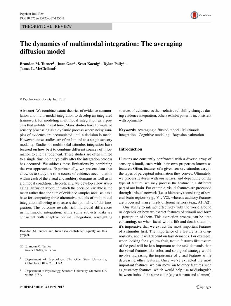
Fig. 1 A comparison of the DDM and the ADM. The left and right panels show a graphical illustration of the evolution of the sensory evidencestate a(t) (x-axis) as a function of time (y-axis) for the DDM (left panel) and the ADM (right panel). For illustrative purposes, we set σw = 0.8,σb = σ0 = 0, and μs = [−1.5, 1.5]
for the DDM. In the beginning, the distribution of evi-dence has relatively little variance, and the location ofpotential belief states are concentrated on μ(t). As timeincreases, the cumulative amount of moment-to-momentnoise increases, which directly impacts the dispersion of thesensory evidence variable a(t). Figure 1 also shows howthese representations interact with the criterion c(t), whichis illustrated by the vertical black line.
Independent of the value of c(t), the level of discrim-inability d ′(t) evolves according to the following equation:
d ′(t) = 2μst
σw
√t
= 2μs
√t
σw
.
As time increases, d ′(t) increases without bound, therebypredicting infinite discriminability (i.e., error-free perfor-mance) at long integration times. While very easy stimuliallow for error-free performance given sufficient process-ing time, the stimuli used in many psychophysical studiesdo not. Yet, the model as stated so far predicts that eventhe most difficult stimuli, if integrated for long enough,should allow error-free performance. There are now threeprominent approaches to addressing this deviation fromoptimality.
First, Ratcliff (1978) proposed that there may be vari-ability from trial to trial in the drift rate parameter. Thatis, a trial-specific value of μ is taken to be sampled froma Gaussian distribution with mean μs and standard devia-tion σb, where σb is referred to as the between-trial driftvariability parameter. While this between-trial variabilitycan be attributed to the stimulus itself, in many studies the
mean stimulus value (e.g., position in screen coordinates)does not vary at all from trial to trial, implying that somefactor internal to the observer (e.g., trial-to-trial variabil-ity in the representation of the reference position) must bethe source of the limitation on performance. Other findings(e.g., Ratcliff and McKoon 2008) suggest that, at the begin-ning of integration, the decision variable may have someinitial variability. Often this is also assumed to be Gaus-sian, with mean 0 and standard deviation σ0. Incorporatingthese additional sources of variability into the DDM, look-ing across many experimental trials, the distribution of theaccumulated evidence variable a(t) still evolves accordingto a normal distribution with mean μ(t) = μst , but itsstandard deviation is
σ(t) =√
σ 20 + σ 2
wt + σ 2b t2. (1)
With these assumptions, it follows that
limt→∞d ′(t) = 2μ
σb
. (2)
In other words, as t increases, the effects of both the ini-tial variability and the moment-to-moment or within-trialvariability become negligible, and accuracy is ultimatelylimited by the between-trial variability. Hence, the addi-tional sources of variability allow the model to account forthe leveling off of accuracy at long decision times.
The second – not mutually exclusive – possibility isthat subjects stop integrating evidence before the end ofa trial once the absolute value of the decision variable

Psychon Bull Rev
a(t) exceeds a decision threshold (Mazurek et al., 2003;Ratcliff, 2006). All models assume some stopping crite-rion for free-response paradigms, when the timing of theresponse is up to the subject. In the interrogation procedure,however, there is no need to stop integrating evidence beforethe go cue occurs, and stopping integration earlier can onlyreduce the discriminability d ′. The use of such a thresholdis still possible however, and it offers one way to explainwhy time-accuracy curves level off. However, we will notinvestigate models that use the thresholding process in thisarticle.
The third possibility is in the way information is inte-grated. While the DDM assumes that the evidence foreach alternative is accumulated in a perfectly anti-correlatedfashion, other models assume a competitive process amongaccumulators where the evidence for each alternative canarrive at different times (Vickers, 1979; Merkle and VanZandt, 2006), inhibit or excite the amount of evidencefor an opposing accumulator (Usher & McClelland, 2001;Brown & Heathcote, 2005; Shadlen & Newsome, 2001),or have a completely independent race process (Brown &Heathcote, 2008; Reddi & Carpenter, 2000). Furthermore,plausible mechanisms such as passive loss of evidence (i.e.,“leakage”) have been considered by other models with sim-ilar accumulation dynamics (Usher & McClelland, 2001;Wong & Wang, 2006). Across various architectures, rangesof parameter settings can allow these models to predict anatural leveling off of the time-accuracy curves. Althoughwe feel that the dynamics of these models are very inter-esting, we will not consider them further in this article.Instead, we will focus on an adaptation of the DDM withstarting-point, between-trial, and within-trial variability asreflected in Eq. 1 as it is very widely used and providesgood descriptive fits to behavioral data (Ratcliff &McKoon,2008).
The averaging diffusion model
We can now adapt the DDM as described above by trans-forming the decision variable into the framework often usedin multisensory integration studies by dividing the amountof accumulated evidence a(t) by the elapsed time t , mea-sured in seconds. We denote this new variable μ̂(t) becauseit is an estimate of the mean of the stimulus variable μ(t).The expected value of μ̂(t) is constant and equal to μs ,while its standard deviation decreases with the square rootof time: σ(t) = σw/
√t . The decrease in the standard
deviation of the estimate of the stimulus variable makes itless and less likely that the evidence value will be on thewrong side of the decision criterion at 0, therefore account-ing for the increase in d ′ as time increases. We call thistransformed version of the DDM the Averaging DiffusionModel (ADM), to represent the fact that the model assumes
participants attempt to estimate the mean of the stimulusinput value.
As in the standard DDM model discussed above, abetween-trial variability parameter σb can allow the ADMto account for limitations in performance (i.e., d ′ reachinga finite asymptotic value) as time increases. Also as in theDDM, the ADM can accommodate initial or starting pointvariability. For our purposes, we assume this initial vari-ability to be drawn from a Gaussian distribution with mean0 and standard deviation σ0. Incorporating these additionalsources of variability into the ADM, the expected value ofthe representation variable a(t) rapidly converges to μs ,while the standard deviation changes as follows:
σ(t) =√
σ 2b + σ 2
w
t+ σ 2
0
t2. (3)
This equation shows that as t increases, the initial variabilityσ0 and the moment-to-moment or within-trial variability σw
become negligible, leading σ(t) to converge to σb, such that
limt→∞d ′(t) = 2μs
σb
. (4)
Hence, as in the DDM, accuracy in the ADM is ultimatelylimited by the between-trial variability, allowing this modelto predict an asymptotic d ′ for large integration times.
The right panel of Fig. 1 illustrates how the distributionof sensory evidence variable a(t) evolves over time for theADM. In the beginning, the distribution of evidence is rel-atively more variable due to the initial starting point noise,making the location of potential beliefs disperse aroundμ(t) due to having only averaged a few noisy samples. Astime increases, the number of noisy samples increases, andthe estimate of the mean of the samples becomes more accu-rate. The model expresses this increased accuracy throughthe decrease in the variance of the representations. Similarto the DDM discussed above, in modeling responses thatoccur at particular times in our behavioral experiment, weassume the participant chooses one response alternative ifthe evidence variable a(t) is greater than a particular crite-rion at the time the response is triggered, and chooses theother response otherwise. In Fig. 1, the criterion c(t) is setto zero and is illustrated by the vertical line in both panels.
Accounting for bias and temporal delay in evidenceintegration
Two additional considerations unrelated to the main focusof our investigation need to be taken into account in pro-viding a complete fit to the experimental data (i.e., allresponse probabilities, not just discriminability data). Thefirst of these is the presence of biases (which vary betweenparticipants) that may favor one response over the other.
Psychon Bull Rev
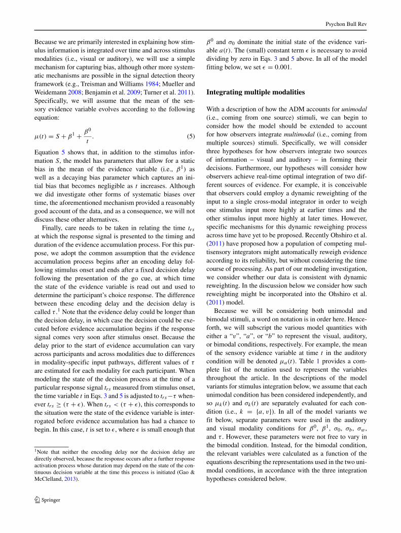
Because we are primarily interested in explaining how stim-ulus information is integrated over time and across stimulusmodalities (i.e., visual or auditory), we will use a simplemechanism for capturing bias, although other more system-atic mechanisms are possible in the signal detection theoryframework (e.g., Treisman and Williams 1984; Mueller andWeidemann 2008; Benjamin et al. 2009; Turner et al. 2011).Specifically, we will assume that the mean of the sen-sory evidence variable evolves according to the followingequation:
μ(t) = S + β1 + β0
t. (5)
Equation 5 shows that, in addition to the stimulus infor-mation S, the model has parameters that allow for a staticbias in the mean of the evidence variable (i.e., β1) aswell as a decaying bias parameter which captures an ini-tial bias that becomes negligible as t increases. Althoughwe did investigate other forms of systematic biases overtime, the aforementioned mechanism provided a reasonablygood account of the data, and as a consequence, we will notdiscuss these other alternatives.
Finally, care needs to be taken in relating the time trsat which the response signal is presented to the timing andduration of the evidence accumulation process. For this pur-pose, we adopt the common assumption that the evidenceaccumulation process begins after an encoding delay fol-lowing stimulus onset and ends after a fixed decision delayfollowing the presentation of the go cue, at which timethe state of the evidence variable is read out and used todetermine the participant’s choice response. The differencebetween these encoding delay and the decision delay iscalled τ .1 Note that the evidence delay could be longer thanthe decision delay, in which case the decision could be exe-cuted before evidence accumulation begins if the responsesignal comes very soon after stimulus onset. Because thedelay prior to the start of evidence accumulation can varyacross participants and across modalities due to differencesin modality-specific input pathways, different values of τ
are estimated for each modality for each participant. Whenmodeling the state of the decision process at the time of aparticular response signal trs measured from stimulus onset,the time variable t in Eqs. 3 and 5 is adjusted to trs−τ when-ever trs ≥ (τ + ε). When trs < (τ + ε), this corresponds tothe situation were the state of the evidence variable is inter-rogated before evidence accumulation has had a chance tobegin. In this case, t is set to ε, where ε is small enough that
1Note that neither the encoding delay nor the decision delay aredirectly observed, because the response occurs after a further responseactivation process whose duration may depend on the state of the con-tinuous decision variable at the time this process is initiated (Gao &McClelland, 2013).
β0 and σ0 dominate the initial state of the evidence vari-able a(t). The (small) constant term ε is necessary to avoiddividing by zero in Eqs. 3 and 5 above. In all of the modelfitting below, we set ε = 0.001.
Integrating multiple modalities
With a description of how the ADM accounts for unimodal(i.e., coming from one source) stimuli, we can begin toconsider how the model should be extended to accountfor how observers integrate multimodal (i.e., coming frommultiple sources) stimuli. Specifically, we will considerthree hypotheses for how observers integrate two sourcesof information – visual and auditory – in forming theirdecisions. Furthermore, our hypotheses will consider howobservers achieve real-time optimal integration of two dif-ferent sources of evidence. For example, it is conceivablethat observers could employ a dynamic reweighting of theinput to a single cross-modal integrator in order to weighone stimulus input more highly at earlier times and theother stimulus input more highly at later times. However,specific mechanisms for this dynamic reweighing processacross time have yet to be proposed. Recently Ohshiro et al.(2011) have proposed how a population of competing mul-tisensory integrators might automatically reweigh evidenceaccording to its reliability, but without considering the timecourse of processing. As part of our modeling investigation,we consider whether our data is consistent with dynamicreweighting. In the discussion below we consider how suchreweighting might be incorporated into the Ohshiro et al.(2011) model.
Because we will be considering both unimodal andbimodal stimuli, a word on notation is in order here. Hence-forth, we will subscript the various model quantities witheither a “v”, “a”, or “b” to represent the visual, auditory,or bimodal conditions, respectively. For example, the meanof the sensory evidence variable at time t in the auditorycondition will be denoted μa(t). Table 1 provides a com-plete list of the notation used to represent the variablesthroughout the article. In the descriptions of the modelvariants for stimulus integration below, we assume that eachunimodal condition has been considered independently, andso μk(t) and σk(t) are separately evaluated for each con-dition (i.e., k = {a, v}). In all of the model variants wefit below, separate parameters were used in the auditoryand visual modality conditions for β0, β1, σ0, σb, σw,and τ . However, these parameters were not free to vary inthe bimodal condition. Instead, for the bimodal condition,the relevant variables were calculated as a function of theequations describing the representations used in the two uni-modal conditions, in accordance with the three integrationhypotheses considered below.

Psychon Bull Rev
Table 1 Model parameters and other variables
Type Notation Description
β0 parameter for component of bias thatdecays over time
Modality β1 parameter representing static bias
Specific σ0 standard deviation of the trial-to-trialstarting point
Parameters σb standard deviation of the trial-to-trialmean drift
σw standard deviation of the within-trial vari-ability
τ the nondecision time parameter
S experimenter-controlled stimulus variable
Condition a(t) the amount of accumulated sensory evi-dence at time t
Specific μ(t) mean of the sensory evidence
Variables σ(t) standard deviation of the sensory evidence
ξ(t) dummy variable used to evaluate pre-dicted response probabilities
Integration α Estimated weight assigned to the visualinput in the SFW model
Variables α∗ optimal value of α for the SOW model
Notation and corresponding description of the parameters and othervariables used throughout the article. All six of the modality-specificparameters of the Averaging Diffusion Model (ADM) were estimatedseparately for the visual and auditory modalities, and all of the con-dition specific variables other that S are calculated separated for thevisual, auditory, and both conditions. Subscripts designating condi-tions are not included for simplicity. SFW: Static Free Weight; SOW:Static Optimal Weight
Hypothesis 1: Adaptive optimal weights
The first method of stimulus integration we investigated wasthe Adaptive Optimal Weights (AOW) model. The AOWmodel assumes that at each time point the observer com-bines the evidence from each of the two modalities in a waythat reflects the reliability of each modality. To do so, themodel relies on a term that expresses the ratio of variabil-ity within a specific modality relative to the total amountof variability in the inputs. For example, the variability inthe auditory representation is σ 2
a (t), whereas the total vari-ability in all the inputs is σ 2
a (t) + σ 2v (t). Hence, the ratio
of these variabilities is σ 2a (t)/
[σ 2
a (t) + σ 2v (t)
]. The intu-
ition behind this term is that as the auditory features of thestimulus become more noisy relative to the visual features,this term increases above 0.5, and as the auditory featuresbecome less noisy relative to the visual features, this termdecreases below 0.5. Using the relation
σ 2a (t)
σ 2a (t) + σ 2
v (t)+ σ 2
v (t)
σ 2a (t) + σ 2
v (t)= 1,
we can use the ratio of variabilities within each modalityto express how cues are combined in an optimal manner(e.g., Ma and Pouget 2008; Landy et al. 2011; Witten andKnudsen 2005). Building on this intuition, in the bimodalcondition, the mean μb(t) and standard deviation σb(t) ofthe stimulus representation are
μb(t) = μv(t)σ 2
a (t)
σ 2a (t) + σ 2
v (t)+ μa(t)
σ 2v (t)
σ 2a (t) + σ 2
v (t)(6)
σb(t) =√
σ 2a (t)σ 2
v (t)
σ 2a (t) + σ 2
v (t). (7)
Hence, the evidence variable in the bimodal conditionab(t) ∼ N (μb(t), σb(t)) will reflect the optimal weightedcombination of the two unimodal evidence variables aa(t)
and av(t). Equations 6 and 7 reflect a cue weighting strategythat is considered “optimal” in the sense that the modalitywith the least amount of variability is given a greater amountof weight when both modalities appear together, as in thebimodal condition. Equations 6 and 7 are also optimal in thesense that they produce the highest possible discriminabilityd ′(t) curve for each value of t .
The weighting terms applied to the visual and auditorymodalities in Eq. 6 may seem counterintuitive given thatthe variance for the visual stream is used in the numera-tor of the weighting term applied to the auditory mean (i.e.,the rightmost term), whereas the variance for the auditorystream appears in the numerator in the term applied to thevisual stream. The reason for this is that the variance in themodality is inversely related to the reliability of the cor-responding modality. As an example, suppose the auditorymodality is perfectly reliable such that σa = 0, and thevisual modality is not perfectly reliable such that σv = q
where q > 0. Here, regardless of the value of q, the weight-ing term applied to the visual modality becomes zero and allattention should go to the auditory modality. This is desir-able in the model because as in this example, the auditorymodality is weighted more heavily, as it is the more reliablemodality.
Hypothesis 2: Static optimal weights
The AOW model above maintains that observers base theirintegration strategy on the reliability of each unimodal fea-ture at the moment the decision must be made. Anotherpossibility is that subjects adopt a single fixed weightingpolicy that maximizes overall response accuracy across allpossible decision times. While the AOW policy will resultin optimal cue weighting at each time point, this alternativepolicy can be considered optimal subject to the constraintthat the weight assigned to each modality is fixed or staticregardless of the reliability of the unimodal evidence at any

Psychon Bull Rev
given moment. We refer to this strategy as the Static OptimalWeight (SOW) model.
For this and the subsequent model, a new parameter α isintroduced. As in the AOW model above, we parameterizethe weights associated with each modality so that they sumto one, or αv + αa = 1. Given this constraint, we (arbitrar-ily) choose α = αv to represent the weight allocated to thevisual modality, such that αa = 1 − α. Since α is assumedfixed for different time points during evidence accumula-tion, we use it to replace the time-specific terms in Eqs. 6and 7 to describe the mean and standard deviation of theevidence variable at time t as
μb(t) = αμv(t) + (1 − α)μa(t), and (8)
σb(t) =√
(ασv(t))2 + ((1 − α)σa(t))2, (9)
respectively.To determine the value of α that maximizes accuracy, we
first define a “response loss function” ξ(t), given by
ξ(t) ={1 − �(0|μb(t), σb(t)) if S > 0�(0|μb(t), σb(t)) if S < 0
(10)
Equation 10 calculates the probability of making a responsefor each of the different values of S, which can take any ofvalues {−2, −1, 1, 2} across trials (S is always the same forboth modalities within a trial). Specifically, if the stimulusis to the right (i.e., S is positive as in Fig. 1), ξ(t) is theproportion of the total area of the sensory evidence distribu-tion that is greater than zero, whereas if the stimulus is tothe left (i.e., S is negative as in Fig. 1), ξ(t) is the propor-tion of the area of the sensory evidence distribution that isless that zero. In both cases, ξ(t) represents the probabilityof making a response that is consistent with the true state ofthe stimulus. In other words, ξ(t) is the probability of mak-ing the correct response. In theory, we could calculate ξ(t)
at every possible time point and select the value of α thatoptimizes ξ(t) for every stimulus value, where
α∗ = argmaxα
(∫ ∞
0ξ(t)dt
). (11)
However, this may not lead to the actual optimal pol-icy given the set of specific time points sampled in ourexperiment. Therefore, we calculate α∗ by summing upthe probabilities at each (discrete) time point used in theexperiment:
α∗ = argmaxα
(∑t
ξ(t)
). (12)
Once α∗ has been determined, it is used in Eqs. 8 and 9 tocalculate μb(t) and σb(t).
Hypothesis 3: Static free weights
The weighting strategies used by the AOW model and theSOW both assume an optimal integration of unimodal cues,and these weighting strategies are both deterministic in thesense that they are completely determined by the parametersfrom the unimodal conditions, carried over directly into thebimodal condition. However, in the presence of two cues,observers may not necessarily integrate them optimally. Inone extreme, they may decide to rely exclusively on onecue over another, since considering both cues simultane-ously may impose extra processing demands on participants(cf. Witten and Knudsen 2005). Given these considera-tions, as well as some of the aforementioned discrepanciesin what is considered optimal, our third model explicitlyparameterizes the weighting process.
The inclusion of this additional model provides for astronger test of optimality of integration. The models con-sidered above are limited in the sense that they provideonly weak evidence about the extent to which a participant’sstrategy is optimal. That is, by assuming a deterministiccombination function, we can only evaluate the fidelityof our assumption by comparing the model fit to empir-ical data, but it does not give us the freedom to explorewhether some other cue-combination strategy is more likelyto account for the data. Because we have data from thisbimodal condition, instead of assuming a direct mappingfrom unimodal conditions to the bimodal one, we can inferthe most-likely weighting policy, conditional on the data.While in principle it is possible that participants choosenon-optimal weights for each value of the decision timeparameter t , considering this possibility would result inexcessive model freedom. Instead we consider the sim-ple possibility that each participant chooses a single valueof the fixed weighting parameter α, corresponding to afixed assignment of weight to signals arising from the audi-tory and visual modalities. As in the SOW model above,we parameterize the weights associated with each modal-ity so that they sum to one, and choose α to represent theweight allocated to the visual modality such that the weightassigned to the auditory modality is 1 − α. As in the SOWmodel, we describe the mean and standard deviation of theevidence variable at time t as
μb(t) = αμv(t) + (1 − α)μa(t), and (13)
σb(t) =√
(ασv(t))2 + ((1 − α)σa(t))2, (14)
respectively. We call this model the Static Free Weights(SFW) model, because the weight α is freely estimated ona subject-by-subject basis, but remains static or fixed for alltime points within each participants’ data.
Psychon Bull Rev
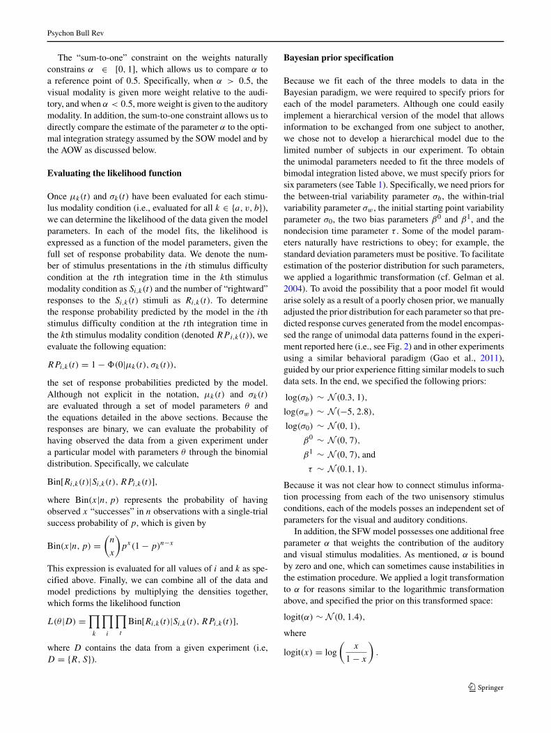
The “sum-to-one” constraint on the weights naturallyconstrains α ∈ [0, 1], which allows us to compare α toa reference point of 0.5. Specifically, when α > 0.5, thevisual modality is given more weight relative to the audi-tory, and when α < 0.5, more weight is given to the auditorymodality. In addition, the sum-to-one constraint allows us todirectly compare the estimate of the parameter α to the opti-mal integration strategy assumed by the SOWmodel and bythe AOW as discussed below.
Evaluating the likelihood function
Once μk(t) and σk(t) have been evaluated for each stimu-lus modality condition (i.e., evaluated for all k ∈ {a, v, b}),we can determine the likelihood of the data given the modelparameters. In each of the model fits, the likelihood isexpressed as a function of the model parameters, given thefull set of response probability data. We denote the num-ber of stimulus presentations in the ith stimulus difficultycondition at the t th integration time in the kth stimulusmodality condition as Si,k(t) and the number of “rightward”responses to the Si,k(t) stimuli as Ri,k(t). To determinethe response probability predicted by the model in the ithstimulus difficulty condition at the t th integration time inthe kth stimulus modality condition (denoted RP i,k(t)), weevaluate the following equation:
RPi,k(t) = 1 − �(0|μk(t), σk(t)),
the set of response probabilities predicted by the model.Although not explicit in the notation, μk(t) and σk(t)
are evaluated through a set of model parameters θ andthe equations detailed in the above sections. Because theresponses are binary, we can evaluate the probability ofhaving observed the data from a given experiment undera particular model with parameters θ through the binomialdistribution. Specifically, we calculate
Bin[Ri,k(t)|Si,k(t), RPi,k(t)],where Bin(x|n, p) represents the probability of havingobserved x “successes” in n observations with a single-trialsuccess probability of p, which is given by
Bin(x|n, p) =(
n
x
)px(1 − p)n−x
This expression is evaluated for all values of i and k as spe-cified above. Finally, we can combine all of the data andmodel predictions by multiplying the densities together,which forms the likelihood function
L(θ |D) =∏k
∏i
∏t
Bin[Ri,k(t)|Si,k(t), RPi,k(t)],
where D contains the data from a given experiment (i.e,D = {R, S}).
Bayesian prior specification
Because we fit each of the three models to data in theBayesian paradigm, we were required to specify priors foreach of the model parameters. Although one could easilyimplement a hierarchical version of the model that allowsinformation to be exchanged from one subject to another,we chose not to develop a hierarchical model due to thelimited number of subjects in our experiment. To obtainthe unimodal parameters needed to fit the three models ofbimodal integration listed above, we must specify priors forsix parameters (see Table 1). Specifically, we need priors forthe between-trial variability parameter σb, the within-trialvariability parameter σw, the initial starting point variabilityparameter σ0, the two bias parameters β0 and β1, and thenondecision time parameter τ . Some of the model param-eters naturally have restrictions to obey; for example, thestandard deviation parameters must be positive. To facilitateestimation of the posterior distribution for such parameters,we applied a logarithmic transformation (cf. Gelman et al.2004). To avoid the possibility that a poor model fit wouldarise solely as a result of a poorly chosen prior, we manuallyadjusted the prior distribution for each parameter so that pre-dicted response curves generated from the model encompas-sed the range of unimodal data patterns found in the experi-ment reported here (i.e., see Fig. 2) and in other experimentsusing a similar behavioral paradigm (Gao et al., 2011),guided by our prior experience fitting similar models to suchdata sets. In the end, we specified the following priors:
log(σb) ∼ N (0.3, 1),
log(σw) ∼ N (−5, 2.8),
log(σ0) ∼ N (0, 1),
β0 ∼ N (0, 7),
β1 ∼ N (0, 7), and
τ ∼ N (0.1, 1).
Because it was not clear how to connect stimulus informa-tion processing from each of the two unisensory stimulusconditions, each of the models posses an independent set ofparameters for the visual and auditory conditions.
In addition, the SFWmodel possesses one additional freeparameter α that weights the contribution of the auditoryand visual stimulus modalities. As mentioned, α is boundby zero and one, which can sometimes cause instabilities inthe estimation procedure. We applied a logit transformationto α for reasons similar to the logarithmic transformationabove, and specified the prior on this transformed space:
logit(α) ∼ N (0, 1.4),
where
logit(x) = log
(x
1 − x
).
Psychon Bull Rev
Ch
oic
e P
ro
ba
bility
Auditory Visual Both
Su
bje
ct
am
0.0 0.5 1.0 1.5 2.0
0.0
0.2
0.4
0.6
0.8
1.0
0.0 0.5 1.0 1.5 2.0
0.0
0.2
0.4
0.6
0.8
1.0
0.0 0.5 1.0 1.5 2.0
0.0
0.2
0.4
0.6
0.8
1.0
Su
bje
ct
hh
0.0 0.5 1.0 1.5 2.0
0.0
0.2
0.4
0.6
0.8
1.0
0.0 0.5 1.0 1.5 2.0
0.0
0.2
0.4
0.6
0.8
1.0
0.0 0.5 1.0 1.5 2.0
0.0
0.2
0.4
0.6
0.8
1.0
Su
bje
ct
jl
0.0 0.5 1.0 1.5 2.0
0.0
0.2
0.4
0.6
0.8
1.0
0.0 0.5 1.0 1.5 2.0
0.0
0.2
0.4
0.6
0.8
1.0
0.0 0.5 1.0 1.5 2.0
0.0
0.2
0.4
0.6
0.8
1.0
Su
bje
ct
la
0.0 0.5 1.0 1.5 2.0
0.0
0.2
0.4
0.6
0.8
1.0
0.0 0.5 1.0 1.5 2.0
0.0
0.2
0.4
0.6
0.8
1.0
0.0 0.5 1.0 1.5 2.0
0.0
0.2
0.4
0.6
0.8
1.0
Su
bje
ct
mb
0.0 0.5 1.0 1.5 2.0
0.0
0.2
0.4
0.6
0.8
1.0
0.0 0.5 1.0 1.5 2.0
0.0
0.2
0.4
0.6
0.8
1.0
0.0 0.5 1.0 1.5 2.0
0.0
0.2
0.4
0.6
0.8
1.0
Su
bje
ct
ms
0.0 0.5 1.0 1.5 2.0
0.0
0.2
0.4
0.6
0.8
1.0
0.0 0.5 1.0 1.5 2.0
0.0
0.2
0.4
0.6
0.8
1.0
0.0 0.5 1.0 1.5 2.0
0.0
0.2
0.4
0.6
0.8
1.0
Go Cue Delay (sec)
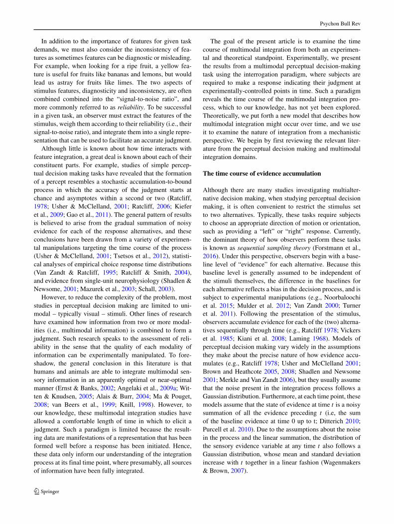
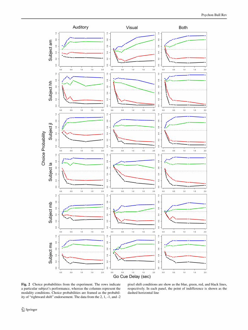
Fig. 2 Choice probabilities from the experiment. The rows indicatea particular subject’s performance, whereas the columns represent themodality conditions. Choice probabilities are framed as the probabil-ity of “rightward shift” endorsement. The data from the 2, 1, -1, and -2
pixel shift conditions are show as the blue, green, red, and black lines,respectively. In each panel, the point of indifference is shown as thedashed horizontal line
Psychon Bull Rev
This particular prior was chosen because it places approxi-mately equal weight for all values of α in the unit interval(i.e., the probability space), and as a consequence, it allowsus to be agnostic about the relative contributions of auditoryand visual stimulus cues in the bimodal stimulus condition.
Experiment
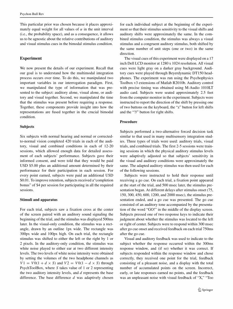
We now present the details of our experiment. Recall thatour goal is to understand how the multimodal integrationprocess occurs over time. To do this, we manipulated twoimportant variables in our interrogation paradigm. First,we manipulated the type of information that was pre-sented to the subject: auditory alone, visual alone, or audi-tory and visual together. Second, we manipulated the timethat the stimulus was present before requiring a response.Together, these components provide insight into how therepresentations are fused together in the crucial bimodalcondition.
Subjects
Six subjects with normal hearing and normal or corrected-to-normal vision completed 420 trials in each of the audi-tory, visual and combined conditions in each of 12-20sessions, which allowed enough data for detailed assess-ment of each subjects’ performance. Subjects gave theirinformed consent, and were told that they would be paidUSD $5.00 plus an additional amount determined by theirperformance for their participation in each session. Forevery point earned, subjects were paid an additional USD$0.01. To improve retention, subjects received a“completionbonus” of $4 per session for participating in all the requiredsessions.
Stimuli and apparatus
For each trial, subjects saw a fixation cross at the centerof the screen paired with an auditory sound signaling thebeginning of the trial, and the stimulus was displayed 500mslater. In the visual-only condition, the stimulus was a rect-angle, drawn by an outline 1px wide. The rectangle was300px wide and 100px high. On each trial, the rectanglestimulus was shifted to either the left or the right by 1 or2 pixels. In the auditory-only condition, the stimulus waswhite noise played to either ear at two different intensitylevels. The two levels of white noise intensity were obtainedby setting the volumes of the two headphone channels asV 1 = V 0(1 + d × S) and V 2 = V 0(1 − d × S) throughPsychToolBox, where S takes value of 1 or 2 representingthe two auditory intensity levels, and d represents the basedifference. The base difference d was adaptively chosen
for each individual subject at the beginning of the experi-ment so that their stimulus sensitivity to the visual shifts andauditory shifts were approximately the same. In the com-bined stimulus condition, the stimulus was always a visualstimulus and a congruent auditory stimulus, both shifted bythe same number of unit steps (one or two) in the samedirection.
The visual cues of this experiment were displayed on a 17inch Dell LCDmonitor at 1280 x 1024 resolution. All visualcues were light gray on a darker gray background. Audi-tory cues were played through Beyerdynamic DT150 head-phones. The experiment was run using the PsychophysicsToolbox v3 extensions of Matlab R2010b. Auditory controlwith precise timing was obtained using M-Audio 1010LTaudio card. Subjects were seated approximately 2.5 feetfrom the computer monitor in the experiment. Subjects wereinstructed to report the direction of the shift by pressing oneof two buttons on the keyboard, the “z” button for left shiftsand the “?/” button for right shifts.
Procedure
Subjects performed a two-alternative forced decision tasksimilar to that used in many multisensory integration stud-ies. Three types of trials were used: auditory trials, visualtrials, and combined trials. The first 2-5 sessions were train-ing sessions in which the physical auditory stimulus levelswere adaptively adjusted so that subjects’ sensitivity inthe visual and auditory conditions were approximately thesame. The adapted auditory stimulus was then used for eachof the following sessions.
Subjects were instructed to hold their response untilreceiving a go cue. On each trial, a fixation point appearedat the start of the trial, and 500 msec later, the stimulus pre-sentation began. At different delays after stimulus onset (75,150, 300, 450, 600, 1200, and 2000 msec), the stimulus pre-sentation ended, and a go cue was presented. The go cueconsisted of an auditory tone accompanied by the presenta-tion of the word “GO!” in the middle of the display screen.Subjects pressed one of two response keys to indicate theirjudgment about whether the stimulus was located to the leftor right of center. Subjects were to respond within 300 msecafter go cue onset and received feedback on each trial 750msafter the go cue.
Visual and auditory feedback was used to indicate to thesubject whether the response occurred within the 300msresponse window, and (if so) whether it was correct. Ifsubjects responded within the response window and chosecorrectly, they received one point for the trial, feedbackconsisting of a pleasant noise, and a display with the totalnumber of accumulated points on the screen. Incorrect,early, or late responses earned no points, and the feedbackwas an unpleasant noise with visual feedback of “X,” “Too

Psychon Bull Rev
early,” or “Too late” on the screen, respectively. The totaltime allotted for feedback of any type was 500ms.
Results
We now present the results of our analysis in five stages.First, we discuss the raw behavioral data because, as wementioned, multimodal integration experiments have notbeen reported with an interrogation paradigm. Second, wediscuss our results in terms of discriminability as mea-sured by signal detection theory model, and compare thesediscriminability measures to ones derived from assumingoptimal integration. Third, we present the results of ourthree model variants, showingmodel fits and model compar-ison statistics. Fourth, we examine the estimated posteriordistribution of the α parameters in our SFW model andcompare them to the optimal setting of α, determined byunimodal feature reliability. Finally, we discuss differencesacross the two modalities in the values of the time offsetparameter τ and the three variability parameters σb, σw,and σ0 and consider how these relate to differences in thetime-accuracy curves for the two modalities.
Raw data
We begin our analysis by examining the raw choice prob-abilities for each modality by shift condition. Figure 2shows the choice probabilities for each subject (rows) bymodality (columns) condition. The choice probabilities areframed as the probability of endorsing the “rightward shift”alternative. The blue, green, red, and black lines repre-sent the choice probabilities for the 2, 1, -1, and -2 pixelshift conditions, respectively, across each of the 7 go cuedelay conditions. In each panel, the point of indifference(i.e., the point at which each response alternative is equallypreferred) is shown as the dashed horizontal line.
Although Fig. 2 shows large individual differences inthe choice probabilities, some features of the data remainconsistent across subjects. First, the larger pixel shift con-ditions result in higher choice probabilities toward the cor-rect alternative, relative to the lower pixel shift conditions.Specifically, the blue and black lines – which represent the2 and -2 pixel shift conditions, respectively – are fartherfrom the point of indifference (0.5) than either the greenor red lines – which represent the 1 and -1 pixel shift con-ditions, respectively. A second general trend in the data isthat the choice probabilities tend to become more discrim-inable (i.e., move away from the point of indifference) as thego cue delay increases. The standard interpretation of thegradual increase in discriminability is that the cumulativesum of the noisy perceptual samples contains more signal
relative to noise over time. Analogously, the ADM pre-sented below describes how the average of these sampleshas a higher signal-to-noise ratio, allowing the representa-tion of the stimulus to be more discriminable over time.
Some features of the data are not consistent across sub-jects. For example, at the shortest go cue delay condition,we see that not all subjects begin at the point of indif-ference. This property suggests that some subjects (e.g.,Subjects hh and la) begin with an initial (rightward choice)bias for reasons that are unlikely to be a consequence ofthe stimuli. Another clear individual difference in the datais the maximum level of response probability for the alter-natives. For example, Subject mb never reaches a responseprobability of 0.8 for the rightward choices under any gocue delay, whereas Subject hh reaches much more extremechoice probabilities for even the shorter go cue delay condi-tions (e.g., a probability of 0.9 at go cue delay 0.6). The rateof response endorsement for each alternative will be morecarefully examined in the next section.
Discriminability analysis and optimality
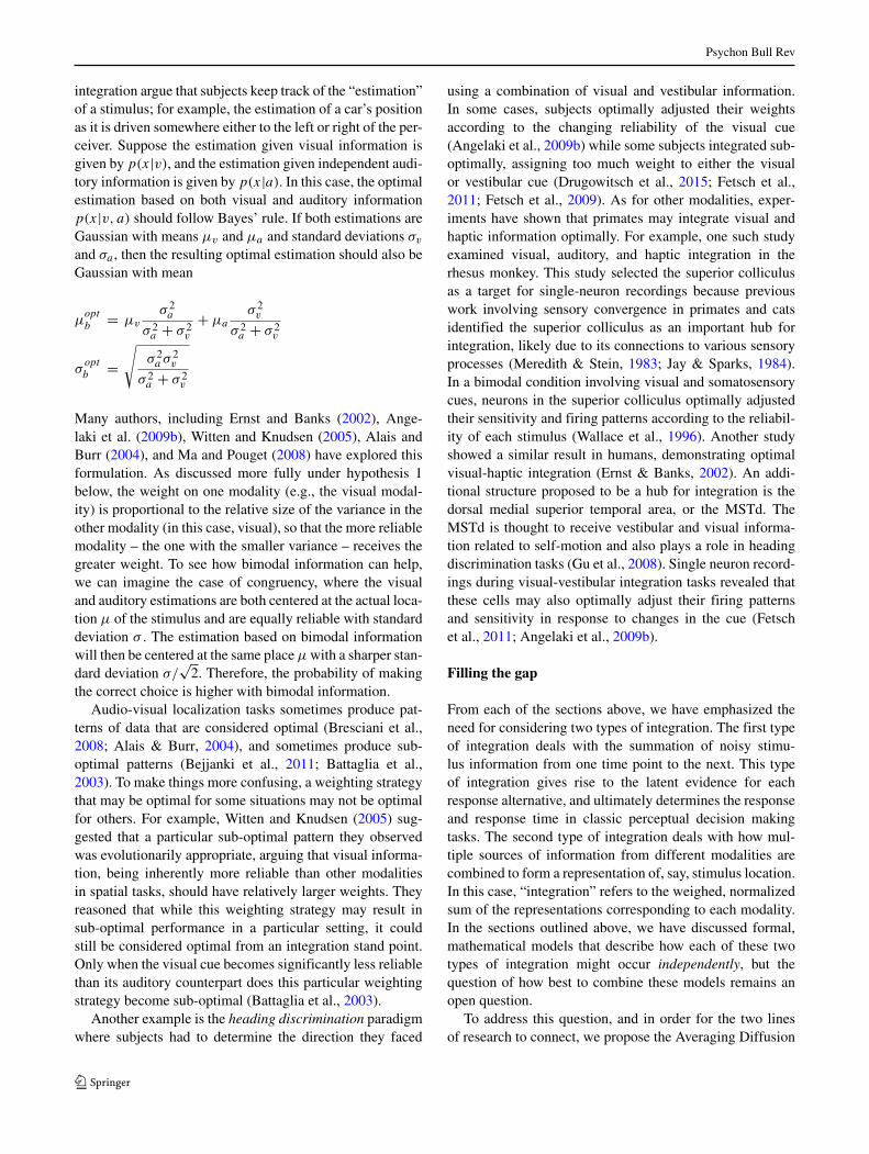
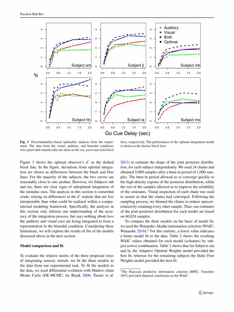
Rather than examining the probability of response endorse-ment, we can rely on summary statistics that characterize thelevel of discriminability for a particular condition. To do thisacross the four stimulus difficulty conditions, we assumedthe presence of four Gaussian distributions, each centered atthe location of the pixel shift conditions [−2, −1, 1, 2]. Wethen assumed that each Gaussian distribution had a standarddeviation parameter equal to σd , and a single decision crite-rion parameter was used as in the traditional signal detectiontheory model (Balakrishnan and MacDonald, 2001). Wethen freely estimated σd and the decision criterion for eachsubject at each interrogation time. Given these assumptions,the level of discriminability for the one-pixel shift conditionis d ′ = 2/σd , whereas discriminability in the two-pixel shiftcondition is d ′ = 4/σd . Figure 3 shows the calculated d ′ val-ues for each subject (shown as panels) in the two-pixel shiftcondition. The green, red, and blue lines represent the d ′curves for the auditory, visual, and both conditions, respec-tively, across all go cue delays. The general pattern acrosssubjects – echoed from Fig. 2 – is that d ′ increases as afunction of the go cue delay.
We can also examine the subjects’ performance relativeto the optimal integration model discussed above. Lettingd ′
v and d ′a denote the discriminability from the visual and
auditory conditions, respectively, the discriminability for theboth condition d ′
b under the assumptions of the optimalintegration model is
d ′b =
√d ′2
a + d ′2v.
Psychon Bull Rev
d'
Subject am Subject jl Subject mb
AuditoryVisualBothOptimal
Subject hh Subject la
0.0 0.5 1.0 1.5 2.0
01
23
4
0.0 0.5 1.0 1.5 2.0
01
23
4
0.0 0.5 1.0 1.5 2.0
01
23
4
0.0 0.5 1.0 1.5 2.0
4
0.0 0.5 1.0 1.5 2.0
01
23
01
23
4
0.0 0.5 1.0 1.5 2.0
01
23
4
Subject ms
Go Cue Delay (sec)Fig. 3 Discriminability-based optimality analysis from the experi-ment. The data from the visual, auditory, and bimodal conditions(two-pixel shift stimuli only) are show as the red, green and solid black
lines, respectively. The performance of the optimal integration modelis shown as the dashed black lines
Figure 3 shows the optimal observer’s d ′ as the dashedblack line. In the figure, deviations from optimal integra-tion are shown as differences between the black and bluelines. For the majority of the subjects, the two curves arereasonably close to one another. However, for Subjects mband ms, there are clear signs of suboptimal integration ofthe stimulus cues. The analysis in this section is somewhatcrude, relying on differences in the d ′ statistic that are lessinterpretable than what could be realized within a compu-tational modeling framework. Specifically, the analysis inthis section only informs our understanding of the accu-racy of the integration process, but says nothing about howthe auditory and visual cues are being integrated to form arepresentation in the bimodal condition. Considering theselimitations, we will explore the results of fits of the modelsdiscussed above in the next section.
Model comparison and fit
To evaluate the relative merits of the three proposed waysof integrating sensory stimuli, we fit the three models tothe data from our experimental task. To fit the models tothe data, we used differential evolution with Markov chainMonte Carlo (DE-MCMC; ter Braak 2006; Turner et al.
2013) to estimate the shape of the joint posterior distribu-tion, for each subject independently. We used 24 chains andobtained 5,000 samples after a burn-in period of 1,000 sam-ples. The burn-in period allowed us to converge quickly tothe high-density regions of the posterior distribution, whilethe rest of the samples allowed us to improve the reliabilityof the estimates. Visual inspection of each chain was usedto assure us that the chains had converged. Following thesampling process, we thinned the chains to reduce autocor-relation by retaining every other sample. Thus, our estimatesof the joint posterior distribution for each model are basedon 60,024 samples.
To compare the three models on the basis of model fit,we used theWatanabe-Akaike information criterion (WAIC;Watanabe 2010).2 For this statistic, a lower value indicatesa better model fit to the data. Table 2 shows the resultingWAIC values obtained for each model (columns) by sub-ject (rows) combination. Table 2 shows that for Subjects amand la, the Adaptive Optimal Weights model provided thebest fit, whereas for the remaining subjects the Static FreeWeights model provided the best fit.
2The Bayesian predictive information criterion (BPIC; Tomohiro2007) provided identical conclusions as the WAIC.
Psychon Bull Rev
Table 2 Watanabe-Akaike information criterion (WAIC) fit statisticsfor each method of stimulus modality integration (columns) by subject(rows)
Subject Adaptive Optimal Static Optimal Static Free
am 1002.5 (79.8) 1087.2 (114.1) 1117.8 (126.9)
hh 599.0 (31.1) 590.1 (30.4) 572.8 (26.2)
jl 645.2 (21.6) 644.6 (22.0) 599.6 (17.5)
la 578.5 (16.5) 587.6 (16.0) 586.7 (14.8)
mb 706.6 (27.1) 705.5 (30.6) 629.1 (18.4)
ms 652.3 (22.5) 590.2 (21.1) 577.0 (15.4)
The standard errors of each WAIC statistic appear in parentheses. Foreach subject, the boldWAIC value indicates the best fitting model
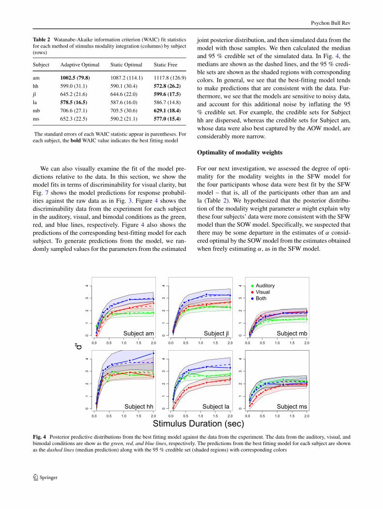
We can also visually examine the fit of the model pre-dictions relative to the data. In this section, we show themodel fits in terms of discriminability for visual clarity, butFig. 7 shows the model predictions for response probabil-ities against the raw data as in Fig. 3. Figure 4 shows thediscriminability data from the experiment for each subjectin the auditory, visual, and bimodal conditions as the green,red, and blue lines, respectively. Figure 4 also shows thepredictions of the corresponding best-fitting model for eachsubject. To generate predictions from the model, we ran-domly sampled values for the parameters from the estimated
joint posterior distribution, and then simulated data from themodel with those samples. We then calculated the medianand 95 % credible set of the simulated data. In Fig. 4, themedians are shown as the dashed lines, and the 95 % credi-ble sets are shown as the shaded regions with correspondingcolors. In general, we see that the best-fitting model tendsto make predictions that are consistent with the data. Fur-thermore, we see that the models are sensitive to noisy data,and account for this additional noise by inflating the 95% credible set. For example, the credible sets for Subjecthh are dispersed, whereas the credible sets for Subject am,whose data were also best captured by the AOW model, areconsiderably more narrow.
Optimality of modality weights
For our next investigation, we assessed the degree of opti-mality for the modality weights in the SFW model forthe four participants whose data were best fit by the SFWmodel – that is, all of the participants other than am andla (Table 2). We hypothesized that the posterior distribu-tion of the modality weight parameter α might explain whythese four subjects’ data were more consistent with the SFWmodel than the SOW model. Specifically, we suspected thatthere may be some departure in the estimates of α consid-ered optimal by the SOWmodel from the estimates obtainedwhen freely estimating α, as in the SFW model.
d' 0.0 0.5 1.0 1.5 2.0
Subject am Subject jl Subject mb
Subject hh Subject la Subject ms
01
23
4
0.0 0.5 1.0 1.5 2.0
01
23
4
0.0 0.5 1.0 1.5 2.0
01
23
4
0.0 0.5 1.0 1.5 2.0
01
23
4
0.0 0.5 1.0 1.5 2.0
01
23
4
0.0 0.5 1.0 1.5 2.0
01
23
4
Stimulus Duration (sec)
Auditory
Both
Visual
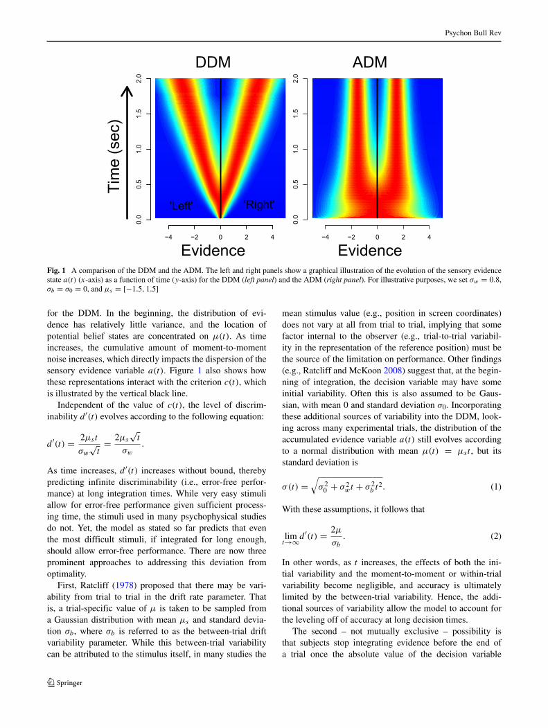
Fig. 4 Posterior predictive distributions from the best fitting model against the data from the experiment. The data from the auditory, visual, andbimodal conditions are show as the green, red, and blue lines, respectively. The predictions from the best fitting model for each subject are shownas the dashed lines (median prediction) along with the 95 % credible set (shaded regions) with corresponding colors
Psychon Bull Rev
α 0.0 0.5 1.0 1.5 2.0
0.0
0.2
0.4
0.6
0.8
1.0
Subject am
SFW
SOW
AOW
0.0 0.5 1.0 1.5 2.0
0.0
0.2
0.4
0.6
0.8
1.0
Subject jl
0.0 0.5 1.0 1.5 2.0
0.0
0.2
0.4
0.6
0.8
1.0
Subject mb
0.0 0.5 1.0 1.5 2.0
0.0
0.2
0.4
0.6
0.8
1.0
Subject hh
0.0 0.5 1.0 1.5 2.0
0.0
0.2
0.4
0.6
0.8
1.0
Subject la
0.0 0.5 1.0 1.5 2.0
0.0
0.2
0.4
0.6
0.8
1.0
Subject ms
Time (sec)
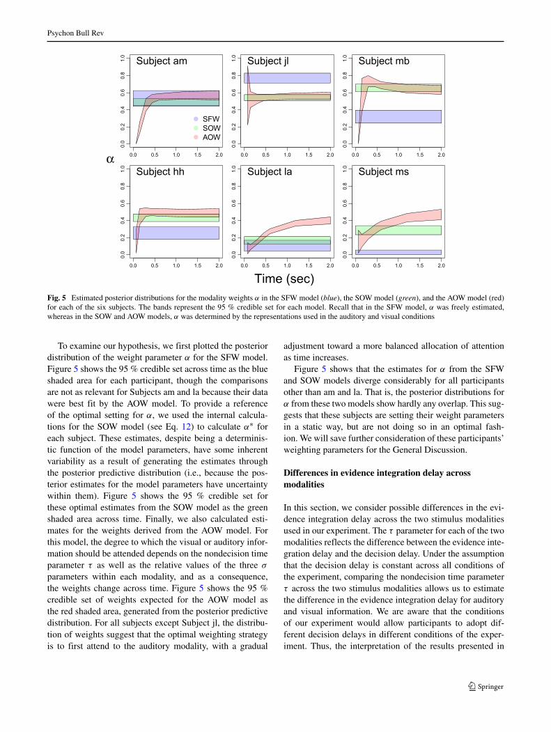
Fig. 5 Estimated posterior distributions for the modality weights α in the SFW model (blue), the SOW model (green), and the AOW model (red)for each of the six subjects. The bands represent the 95 % credible set for each model. Recall that in the SFW model, α was freely estimated,whereas in the SOW and AOW models, α was determined by the representations used in the auditory and visual conditions
To examine our hypothesis, we first plotted the posteriordistribution of the weight parameter α for the SFW model.Figure 5 shows the 95 % credible set across time as the blueshaded area for each participant, though the comparisonsare not as relevant for Subjects am and la because their datawere best fit by the AOW model. To provide a referenceof the optimal setting for α, we used the internal calcula-tions for the SOW model (see Eq. 12) to calculate α∗ foreach subject. These estimates, despite being a determinis-tic function of the model parameters, have some inherentvariability as a result of generating the estimates throughthe posterior predictive distribution (i.e., because the pos-terior estimates for the model parameters have uncertaintywithin them). Figure 5 shows the 95 % credible set forthese optimal estimates from the SOW model as the greenshaded area across time. Finally, we also calculated esti-mates for the weights derived from the AOW model. Forthis model, the degree to which the visual or auditory infor-mation should be attended depends on the nondecision timeparameter τ as well as the relative values of the three σ
parameters within each modality, and as a consequence,the weights change across time. Figure 5 shows the 95 %credible set of weights expected for the AOW model asthe red shaded area, generated from the posterior predictivedistribution. For all subjects except Subject jl, the distribu-tion of weights suggest that the optimal weighting strategyis to first attend to the auditory modality, with a gradual
adjustment toward a more balanced allocation of attentionas time increases.
Figure 5 shows that the estimates for α from the SFWand SOW models diverge considerably for all participantsother than am and la. That is, the posterior distributions forα from these two models show hardly any overlap. This sug-gests that these subjects are setting their weight parametersin a static way, but are not doing so in an optimal fash-ion. We will save further consideration of these participants’weighting parameters for the General Discussion.
Differences in evidence integration delay acrossmodalities
In this section, we consider possible differences in the evi-dence integration delay across the two stimulus modalitiesused in our experiment. The τ parameter for each of the twomodalities reflects the difference between the evidence inte-gration delay and the decision delay. Under the assumptionthat the decision delay is constant across all conditions ofthe experiment, comparing the nondecision time parameterτ across the two stimulus modalities allows us to estimatethe difference in the evidence integration delay for auditoryand visual information. We are aware that the conditionsof our experiment would allow participants to adopt dif-ferent decision delays in different conditions of the exper-iment. Thus, the interpretation of the results presented in
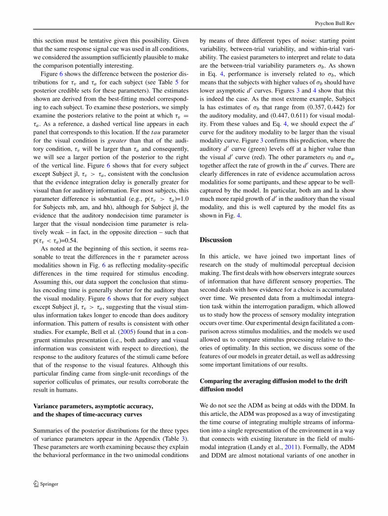
Psychon Bull Rev
this section must be tentative given this possibility. Giventhat the same response signal cue was used in all conditions,we considered the assumption sufficiently plausible to makethe comparison potentially interesting.
Figure 6 shows the difference between the posterior dis-tributions for τv and τa for each subject (see Table 5 forposterior credible sets for these parameters). The estimatesshown are derived from the best-fitting model correspond-ing to each subject. To examine these posteriors, we simplyexamine the posteriors relative to the point at which τv =τa . As a reference, a dashed vertical line appears in eachpanel that corresponds to this location. If the tau parameterfor the visual condition is greater than that of the audi-tory condition, τv will be larger than τa and consequently,we will see a larger portion of the posterior to the rightof the vertical line. Figure 6 shows that for every subjectexcept Subject jl, τv > τa , consistent with the conclusionthat the evidence integration delay is generally greater forvisual than for auditory information. For most subjects, thisparameter difference is substantial (e.g., p(τv > τa)=1.0for Subjects mb, am, and hh), although for Subject jl, theevidence that the auditory nondecision time parameter islarger that the visual nondecision time parameter is rela-tively weak – in fact, in the opposite direction – such thatp(τv < τa)=0.54.
As noted at the beginning of this section, it seems rea-sonable to treat the differences in the τ parameter acrossmodalities shown in Fig. 6 as reflecting modality-specificdifferences in the time required for stimulus encoding.Assuming this, our data support the conclusion that stimu-lus encoding time is generally shorter for the auditory thanthe visual modality. Figure 6 shows that for every subjectexcept Subject jl, τv > τa , suggesting that the visual stim-ulus information takes longer to encode than does auditoryinformation. This pattern of results is consistent with otherstudies. For example, Bell et al. (2005) found that in a con-gruent stimulus presentation (i.e., both auditory and visualinformation was consistent with respect to direction), theresponse to the auditory features of the stimuli came beforethat of the response to the visual features. Although thisparticular finding came from single-unit recordings of thesuperior colliculus of primates, our results corroborate theresult in humans.
Variance parameters, asymptotic accuracy,and the shapes of time-accuracy curves
Summaries of the posterior distributions for the three typesof variance parameters appear in the Appendix (Table 3).These parameters are worth examining because they explainthe behavioral performance in the two unimodal conditions
by means of three different types of noise: starting pointvariability, between-trial variability, and within-trial vari-ability. The easiest parameters to interpret and relate to dataare the between-trial variability parameters σb. As shownin Eq. 4, performance is inversely related to σb, whichmeans that the subjects with higher values of σb should havelower asymptotic d ′ curves. Figures 3 and 4 show that thisis indeed the case. As the most extreme example, Subjectla has estimates of σb that range from (0.357, 0.442) forthe auditory modality, and (0.447, 0.611) for visual modal-ity. From these values and Eq. 4, we should expect the d ′curve for the auditory modality to be larger than the visualmodality curve. Figure 3 confirms this prediction, where theauditory d ′ curve (green) levels off at a higher value thanthe visual d ′ curve (red). The other parameters σ0 and σw
together affect the rate of growth in the d ′ curves. There areclearly differences in rate of evidence accumulation acrossmodalities for some partipants, and these appear to be well-captured by the model. In particular, both am and la showmuch more rapid growth of d ′ in the auditory than the visualmodality, and this is well captured by the model fits asshown in Fig. 4.
Discussion
In this article, we have joined two important lines ofresearch on the study of multimodal perceptual decisionmaking. The first deals with how observers integrate sourcesof information that have different sensory properties. Thesecond deals with how evidence for a choice is accumulatedover time. We presented data from a multimodal integra-tion task within the interrogation paradigm, which allowedus to study how the process of sensory modality integrationoccurs over time. Our experimental design facilitated a com-parison across stimulus modalities, and the models we usedallowed us to compare stimulus processing relative to the-ories of optimality. In this section, we discuss some of thefeatures of our models in greater detail, as well as addressingsome important limitations of our results.
Comparing the averaging diffusion model to the driftdiffusion model
We do not see the ADM as being at odds with the DDM. Inthis article, the ADMwas proposed as a way of investigatingthe time course of integrating multiple streams of informa-tion into a single representation of the environment in a waythat connects with existing literature in the field of multi-modal integration (Landy et al., 2011). Formally, the ADMand DDM are almost notational variants of one another in

Psychon Bull Rev
De
nsity
Subject amp(τv > τa)=1.00
010
20
30
40
Subject jlp(τv > τa)=0.46
Subject mbp(τv > τa)=1.00
Subject hhp(τv > τa)=1.00
010
20
30
40
Subject lap(τv > τa)=0.89
−0.10 0.00 0.10 0.20
010
20
30
40
−0.10 0.00 0.10 0.20 −0.10 0.00 0.10 0.20
010
20
30
40
−0.10 0.00 0.10 0.20
01
02
03
04
0
−0.10 0.00 0.10 0.20 −0.10 0.00 0.10 0.20
01
02
03
04
0
Subject msp(τv a)=0.66
τv
> τ
− τa (sec)
Fig. 6 A comparison across modalities of the estimated posterior distribution for the nondecision time parameter τ . Each panel shows thedifference in τ between visual and auditory stimulus modalities for the best fitting model for each subject. Reference lines appear in each panelfor the point at which the two nondecision time parameters are equal. The units of τ are in seconds
the absence of a decision bound. As we discussed in theintroduction, both the mean and standard deviation of theevidence variable in the DDM are simply divided by t toobtain the mean and standard deviation of the evidence vari-able in the ADM. As a consequence, when diving the meanby the standard deviation, as one would when calculatingthe signal-to-noise ratio, the resulting d ′ measures are iden-tical across the two models because d ′(t) is proportional toμ(t)/σ (t) (see Eqs. 2 and 4).
The advantage of developing the ADM is that it can beextended to task in which participants are asked to indicatetheir estimate of the position of the stimulus on a contin-uum, as reflected in the ADM’s evidence variable a(t). Suchextensions are in line with recent developments of the DDMfor continuous elicitation paradigms (Smith, 2016).
Our experiment used an exogenous stopping rule viathe interrogation paradigm where subjects were requiredto respond immediately following a go cue. While thisparadigm is useful in understanding how the sensory vari-ables evolve over time, as presented here, the model is notsuited for endogenous stopping rules where subjects deter-mine when a choice should be made. These paradigms,often referred to as “free response” paradigms, are concep-tually quite similar to interrogation paradigms, but mod-els of this task require some mechanism to terminate the
information accumulation process. Typically, the termina-tion process is instantiated in a decision model such as theDDM through a response threshold parameter. Although ithas been argued that a response threshold mechanism couldunderly the decision dynamics in the interrogation paradigm(see Ratcliff 2006), we have ignored this possibility herebecause excellent fits to time-accuracy curves are oftenobtained without such a mechanism (see, e.g., Gao et al.2011, for a study that used a procedure very similar to theone used here). Because including the possibility of an earlytermination policy (i.e., prior to the go cue) would greatlyincrease the complexity of the ADM presented here, weopted for the simpler formulation in which the decision vari-able remains continuous until readout is triggered by the gocue. Future work could investigate ‘the incorporation of adecision bound into’ the ADM.
Weight parameters, optimality, and neglect
One surprising result from our analyses was the lack ofoptimality in the decision making process for four out ofour six subjects. Recall that we used two different defi-nitions of optimality when constructing variants of ADM.First, we used the classic definition of optimality whereweights are established on the basis of the variability (i.e.,
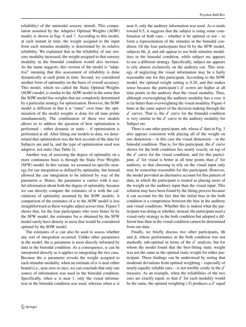
Psychon Bull Rev
reliability) of the unimodal sensory stimuli. This compu-tation assumed by the Adaptive Optimal Weights (AOW)model, is shown in Eqs. 6 and 7. According to this model,at each instant in time, the weight assigned to the inputfrom each stimulus modality is determined by its relativereliability. We explained that as the reliability of one sen-sory modality increased, the weight assigned to that sensorymodality in the bimodal condition would also increase.As the name suggests, this version of the model is “adap-tive” meaning that this assessment of reliability is donedynamically at each point in time. Second, we consideredanother form of optimality on the basis of overall accuracy.This model, which we called the Static Optimal Weights(SOW) model, is similar to the AOWmodel in the sense thatthe SOWmodel has weights that are completely determinedby a particular strategy for optimization. However, the SOWmodel is different in that it is “static” over time: the opti-mization of the model weights is done for all time pointssimultaneously. The combination of these two modelsallows us to address the question of how optimization isperformed – either dynamic or static – if optimization isperformed at all. After fitting our models to data, we deter-mined that optimization was the best account of the data forSubjects am and la, and the type of optimization used wasadaptive, not static (See Table 2).
Another way of assessing the degree of optimality on amore continuous basis is through the Static Free Weights(SFW) model. In this variant, we assumed no specific strat-egy for cue integration as defined by optimality, but insteadallowed the cue integration to be inferred by way of theparameter α. Hence, the parameter α carries with it use-ful information about both the degree of optimality, becausewe can directly compare the estimates of α with the cal-culations of optimality assumed by the SOW models. Acomparison of the estimates of α to the AOW model is lessstraightforward as these weights adjust across time. Figure 5shows that, for the four participants who were better fit bythe SFW model, the estimates for α obtained by the SFWmodel rarely have density in areas that would be consideredoptimal by the SOW model.
The estimates of α can also be used to assess whetherany sort of integration occurred. Unlike other parametersin the model, the α parameter is most directly informed bydata in the bimodal condition. As a consequence, α can beinterpreted directly as it applies to integrating the two cues.Because the α parameter reveals the weight assigned toeach stimulus modality, when an estimate of α is near eitherbound (i.e., near zero or one), we can conclude that only onesource of information was used in the bimodal condition.Specifically, when α is near 1, only the visual informa-tion in the bimodal condition was used, whereas when α is
near 0, only the auditory information was used. As α tendstoward 0.5, it suggests that the subject is using some com-bination of both cues – whether it be optimal or not – toform a representation of the stimulus in the bimodal con-dition. Of the four participants best fit by the SFW model,subjects hh, jl, and mb appear to use both stimulus modal-ities in the bimodal condition, whils subject ms appearsto use a different strategy. Specifically, subject ms appearsto rely almost exclusively on the auditory cue. This strat-egy of neglecting the visual information may be a fairlyreasonable one for this participant. According to the SOWmodel, the optimal weight setting is 0.28, and this makessense because the participant’s d’ scores are higher at alltime points in the auditory than the visual modality. Thus,although overweighting the auditory modality has a cost, itis far better than overweighting the visual modality. Figure 4hints at the same aspect of the decision making through thed ′ curves. That is, the d ′ curve for the bimodal conditionis very similar to the d ′ curve in the auditory modality forSubject ms.
There is one other participant, mb, whose d ′ data in Fig. 3also appears consistent with placing all of the weight onone dimension – in this case the visual dimension – in thebimodal condition. That is, for this participant, the d ′ curveshown for the both condition lies nearly exactly on top ofthe d ′ curve for the visual condition, and for this partici-pant, d ′ for visual is better at all time points than d ′ forauditory, so that choosing to rely on the visual input onlymay be somewhat reasonable for this participant. However,the model provided an alternative account for this pattern ofdata, in which the participant is treated as placing more ofthe weight on the auditory input than the visual input. Thissolution may have been found by the fitting process becauseit can account for the fact that the initial bias in the bothcondition is a compromise between the bias in the auditoryand visual conditions. Whether this is indeed what the par-ticipant was doing or whether, instead, the participant used avisual-only strategy in the both condition but adopted a dif-ferent bias than in the visual condition cannot be determinedfrom our data.
Finally, we briefly discuss two other participants, hhand jl, whose performance in the both condition was notmarkedly sub-optimal in terms of the d ′ analysis, but forwhom the model found that the best-fitting static weightwas not the same as the optimal static weight for either par-ticipant. These findings can be understood by noting thatmoderate deviations from optimal weighting – especially ofnearly-equally reliable cues – is not terribly costly in the d ′measure. As an example, when the reliabilities of the twocues are exactly equal, so that d ′ for each modality wouldbe the same, the optimal weighting (.5) produces a d ′ equal
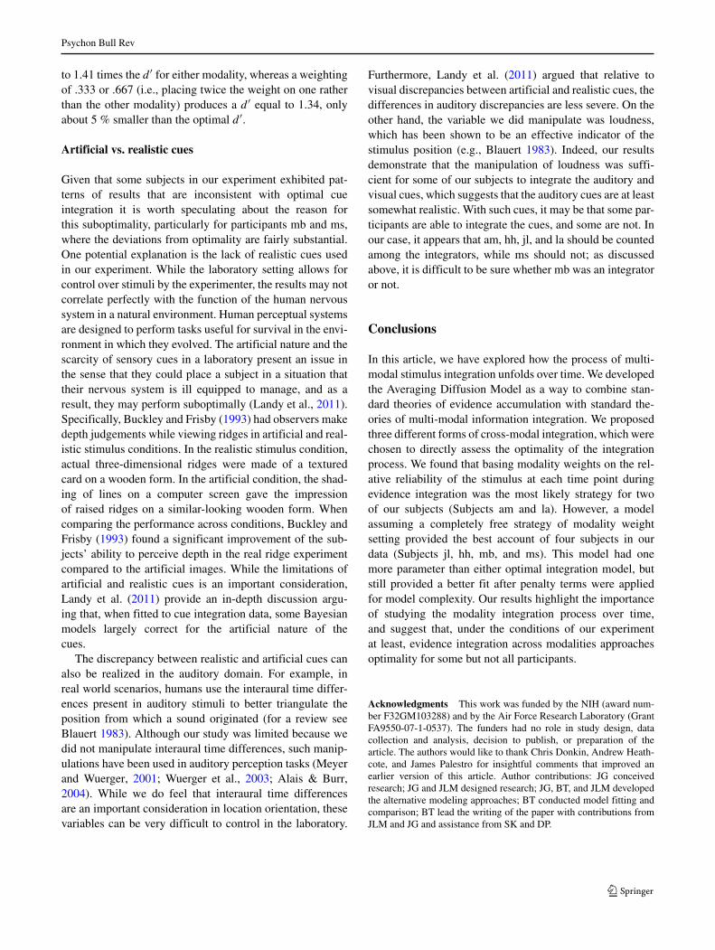
Psychon Bull Rev
to 1.41 times the d ′ for either modality, whereas a weightingof .333 or .667 (i.e., placing twice the weight on one ratherthan the other modality) produces a d ′ equal to 1.34, onlyabout 5 % smaller than the optimal d ′.
Artificial vs. realistic cues
Given that some subjects in our experiment exhibited pat-terns of results that are inconsistent with optimal cueintegration it is worth speculating about the reason forthis suboptimality, particularly for participants mb and ms,where the deviations from optimality are fairly substantial.One potential explanation is the lack of realistic cues usedin our experiment. While the laboratory setting allows forcontrol over stimuli by the experimenter, the results may notcorrelate perfectly with the function of the human nervoussystem in a natural environment. Human perceptual systemsare designed to perform tasks useful for survival in the envi-ronment in which they evolved. The artificial nature and thescarcity of sensory cues in a laboratory present an issue inthe sense that they could place a subject in a situation thattheir nervous system is ill equipped to manage, and as aresult, they may perform suboptimally (Landy et al., 2011).Specifically, Buckley and Frisby (1993) had observers makedepth judgements while viewing ridges in artificial and real-istic stimulus conditions. In the realistic stimulus condition,actual three-dimensional ridges were made of a texturedcard on a wooden form. In the artificial condition, the shad-ing of lines on a computer screen gave the impressionof raised ridges on a similar-looking wooden form. Whencomparing the performance across conditions, Buckley andFrisby (1993) found a significant improvement of the sub-jects’ ability to perceive depth in the real ridge experimentcompared to the artificial images. While the limitations ofartificial and realistic cues is an important consideration,Landy et al. (2011) provide an in-depth discussion argu-ing that, when fitted to cue integration data, some Bayesianmodels largely correct for the artificial nature of thecues.
The discrepancy between realistic and artificial cues canalso be realized in the auditory domain. For example, inreal world scenarios, humans use the interaural time differ-ences present in auditory stimuli to better triangulate theposition from which a sound originated (for a review seeBlauert 1983). Although our study was limited because wedid not manipulate interaural time differences, such manip-ulations have been used in auditory perception tasks (Meyerand Wuerger, 2001; Wuerger et al., 2003; Alais & Burr,2004). While we do feel that interaural time differencesare an important consideration in location orientation, thesevariables can be very difficult to control in the laboratory.
Furthermore, Landy et al. (2011) argued that relative tovisual discrepancies between artificial and realistic cues, thedifferences in auditory discrepancies are less severe. On theother hand, the variable we did manipulate was loudness,which has been shown to be an effective indicator of thestimulus position (e.g., Blauert 1983). Indeed, our resultsdemonstrate that the manipulation of loudness was suffi-cient for some of our subjects to integrate the auditory andvisual cues, which suggests that the auditory cues are at leastsomewhat realistic. With such cues, it may be that some par-ticipants are able to integrate the cues, and some are not. Inour case, it appears that am, hh, jl, and la should be countedamong the integrators, while ms should not; as discussedabove, it is difficult to be sure whether mb was an integratoror not.
Conclusions
In this article, we have explored how the process of multi-modal stimulus integration unfolds over time. We developedthe Averaging Diffusion Model as a way to combine stan-dard theories of evidence accumulation with standard the-ories of multi-modal information integration. We proposedthree different forms of cross-modal integration, which werechosen to directly assess the optimality of the integrationprocess. We found that basing modality weights on the rel-ative reliability of the stimulus at each time point duringevidence integration was the most likely strategy for twoof our subjects (Subjects am and la). However, a modelassuming a completely free strategy of modality weightsetting provided the best account of four subjects in ourdata (Subjects jl, hh, mb, and ms). This model had onemore parameter than either optimal integration model, butstill provided a better fit after penalty terms were appliedfor model complexity. Our results highlight the importanceof studying the modality integration process over time,and suggest that, under the conditions of our experimentat least, evidence integration across modalities approachesoptimality for some but not all participants.
Acknowledgments This work was funded by the NIH (award num-ber F32GM103288) and by the Air Force Research Laboratory (GrantFA9550-07-1-0537). The funders had no role in study design, datacollection and analysis, decision to publish, or preparation of thearticle. The authors would like to thank Chris Donkin, Andrew Heath-cote, and James Palestro for insightful comments that improved anearlier version of this article. Author contributions: JG conceivedresearch; JG and JLM designed research; JG, BT, and JLM developedthe alternative modeling approaches; BT conducted model fitting andcomparison; BT lead the writing of the paper with contributions fromJLM and JG and assistance from SK and DP.

Psychon Bull Rev
Appendix
Table 3 Estimates for Variance Parameters. Posterior summaries for the three variance parameters in the auditory and visual modalities for thebest fitting model for each subject
Auditory Visual
Subject σb σw σ0 σb σw σ0
am (1.977, 2.277) (0.000, 0.383) (0.468, 0.848) (1.530, 1.771) (0.000, 0.144) (0.576, 0.845)
hh (1.229, 1.428) (0.000, 0.508) (0.188, 0.347) (1.283, 1.481) (0.000, 0.196) (0.203, 0.303)
jl (1.595, 1.819) (0.000, 0.307) (0.360, 0.587) (1.411, 1.578) (0.000, 0.458) (0.387, 0.547)
la (1.429, 1.556) (0.000, 0.287) (0.183, 0.270) (1.563, 1.842) (0.000, 0.533) (0.775, 1.125)
mb (2.642, 3.181) (0.000, 0.666) (0.954, 1.568) (2.063, 2.426) (0.000, 0.486) (0.318, 0.627)
ms (1.721, 1.954) (0.000, 0.352) (0.390, 0.730) (1.615, 2.113) (0.000, 0.561) (0.930, 1.758)
Each summary presents the 95 % credible set for each parameter. Values less than 0.0005 were rounded to 0.000
Table 4 Estimates for Bias Parameters. Posterior summaries for the two bias parameters in the auditory and visual modalities for the best fittingmodel for each subject
Auditory Visual
Subject β0 β1 β0 β1
am (−0.086, −0.012) (0.271, 0.485) (−0.290, −0.165) (−0.267, −0.022)
hh (0.087, 0.150) (−0.392, −0.225) (0.167, 0.248) (−1.106, −0.877)
jl (−0.042, 0.011) (0.376, 0.550) (0.061, 0.113) (−0.617, −0.465)
la (0.088, 0.136) (−0.448, −0.311) (0.301, 0.477) (−0.735, −0.503)
mb (−0.262, −0.119) (−0.158, 0.122) (−0.026, 0.018) (−1.040, −0.826)
ms (0.037, 0.116) (−0.073, 0.108) (−0.222, −0.021) (0.144, 0.488)
Each summary presents the 95 % credible set for each parameter
Table 5 Estimates for Nondecision Time Parameters. Posterior sum-maries for the nondecision time parameters in the auditory and visualmodalities for the best fitting model for each subject
Subject Auditory τ Visual τ
am (−0.065, 0.021) (0.074, 0.123)
hh (0.022, 0.059) (0.056, 0.072)
jl (0.009, 0.064) (0.019, 0.054)
la (0.017, 0.043) (0.016, 0.093)
mb (−0.021, 0.062) (0.072, 0.118)
ms (−0.087, 0.012) (−0.107, 0.049)
Each summary presents the 95 % credible set for each parameter
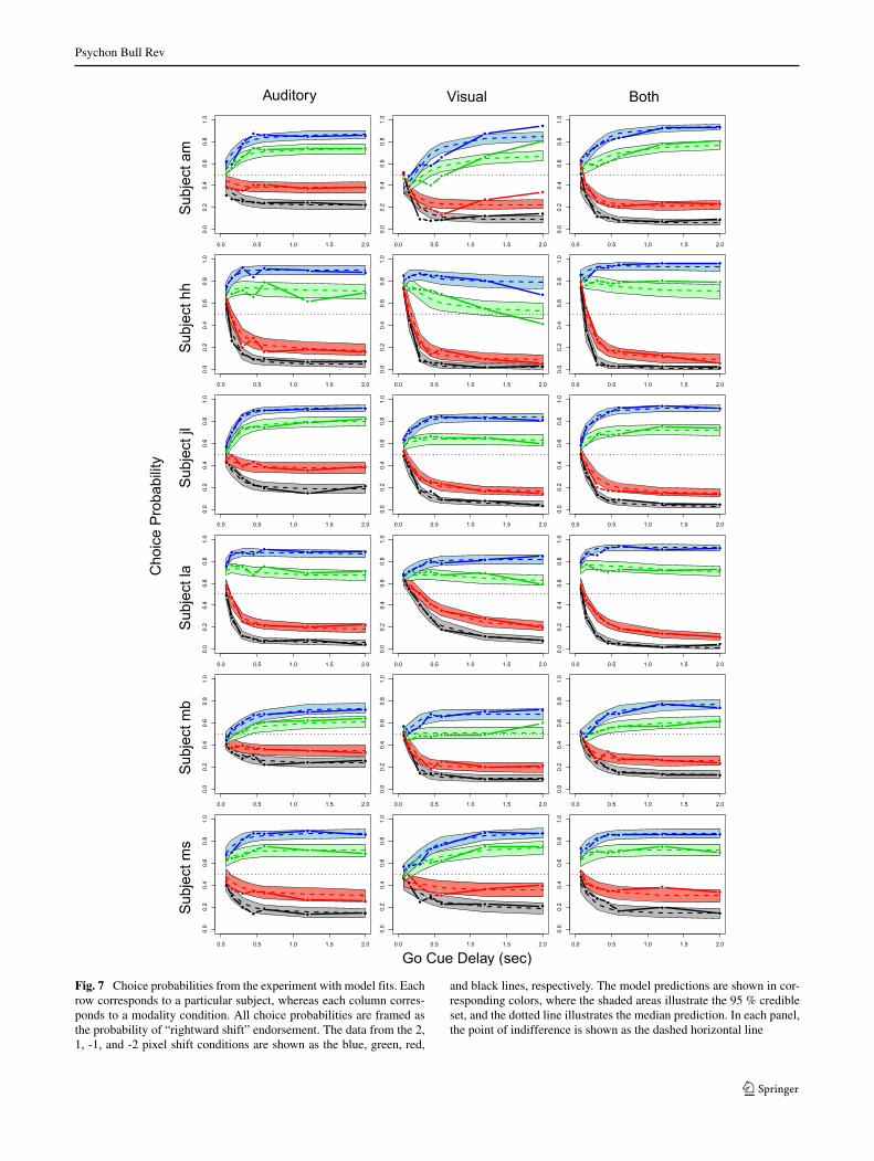
Psychon Bull Rev
Ch
oic
e P
ro
ba
bility
Auditory Visual Both
Su
bje
ct
am
0.0 0.5 1.0 1.5 2.0
0.0
0.2
0.4
0.6
0.8
1.0
0.0 0.5 1.0 1.5 2.0
0.0
0.2
0.4
0.6
0.8
1.0
0.0 0.5 1.0 1.5 2.0
0.0
0.2
0.4
0.6
0.8
1.0
Su
bje
ct
hh
0.0 0.5 1.0 1.5 2.0
0.0
0.2
0.4
0.6
0.8
1.0
0.0 0.5 1.0 1.5 2.0
0.0
0.2
0.4
0.6
0.8
1.0
0.0 0.5 1.0 1.5 2.0
0.0
0.2
0.4
0.6
0.8
1.0
Su
bje
ct
jl
0.0 0.5 1.0 1.5 2.0
0.0
0.2
0.4
0.6
0.8
1.0
0.0 0.5 1.0 1.5 2.0
0.0
0.2
0.4
0.6
0.8
1.0
0.0 0.5 1.0 1.5 2.0
0.0
0.2
0.4
0.6
0.8
1.0
Su
bje
ct
la
0.0 0.5 1.0 1.5 2.0
0.0
0.2
0.4
0.6
0.8
1.0
0.0 0.5 1.0 1.5 2.0
0.0
0.2
0.4
0.6
0.8
1.0
0.0 0.5 1.0 1.5 2.0
0.0
0.2
0.4
0.6
0.8
1.0
Su
bje
ct
mb
0.0 0.5 1.0 1.5 2.0
0.0
0.2
0.4
0.6
0.8
1.0
0.0 0.5 1.0 1.5 2.0
0.0
0.2
0.4
0.6
0.8
1.0
0.0 0.5 1.0 1.5 2.0
0.0
0.2
0.4
0.6
0.8
1.0
Su
bje
ct
ms
0.0 0.5 1.0 1.5 2.0
0.0
0.2
0.4
0.6
0.8
1.0
0.0 0.5 1.0 1.5 2.0
0.0
0.2
0.4
0.6
0.8
1.0
0.0 0.5 1.0 1.5 2.0
0.0
0.2
0.4
0.6
0.8
1.0
Go Cue Delay (sec)
Fig. 7 Choice probabilities from the experiment with model fits. Eachrow corresponds to a particular subject, whereas each column corres-ponds to a modality condition. All choice probabilities are framed asthe probability of “rightward shift” endorsement. The data from the 2,1, -1, and -2 pixel shift conditions are shown as the blue, green, red,
and black lines, respectively. The model predictions are shown in cor-responding colors, where the shaded areas illustrate the 95 % credibleset, and the dotted line illustrates the median prediction. In each panel,the point of indifference is shown as the dashed horizontal line

Psychon Bull Rev
References
Alais, D., & Burr, D. (2004). The ventriloquist effect results from near-optimal bimodal integration. Current Biology, 14, 257–262.
Angelaki, D.E., Gu, Y., & DeAngelis, G.C. (2009a). Multisensoryintegration: psychophysics, neurophysiology, and computation.Current Opinion in Neurobiology, 19, 452–458.
Angelaki, D.E., Klier, E.M., & Snyder, E.H. (2009b). A vestibular sen-sation: probabilistic approaches to spatial perception. Neuron, 64,448–461.
Balakrishnan, J., & MacDonald, J. (2001). Alternatives, misrepresen-tations of signal detection theory and an alternative approach tohuman image classification. Journal of Electronic Imaging, 10,376–384.
Battaglia, P.W., Jacobs, R.A., & Aslin, R.N. (2003). Bayesian integra-tion of visual and auditory signals for spatial localization. Journalof the Optical Society of America, 20, 1391–1397.
Bejjanki, V.R., Clayards, M., Knill, D.C., & Aslin, R.N. (2011). Cueintegration in categorical tasks: Insights from audio-visual speechperception. PloS One, 6, 1–12.
Bell, A., Meredith, A., Van Opstal, A.J., & Munoz, D.P. (2005). Cross-modal integration in the primate superior colliculus underlying thepreparation and initiation of saccadic eye movements. Journal ofNeurophysiology, 93, 3659–3673.
Benjamin, A.S., Diaz, M., &Wee, S. (2009). Signal detection with cri-terior noise: Applications to recognition memory. PsychologicalReview, 116, 84–115.
Blauert, J. (Ed.) (1983). Spatial Hearing. Cambridge: MIT Press.Bresciani, J.-P., Dammeier, F., & Ernst, M.O. (2008). Tri-modal inte-
gration of visual, tactile, and auditory signals for the perception ofsequences of events. Brain Research Bulletin, 75, 753–760.
Brown, S., & Heathcote, A. (2005). A ballistic model of choiceresponse time. Psychological Review, 112, 117–128.
Brown, S., & Heathcote, A. (2008). The simplest complete modelof choice reaction time: Linear ballistic accumulation. CognitivePsychology, 57, 153–178.
Buckley, D., & Frisby, J.P. (1993). Interaction of stereo, texture andoutline cues in the shape perception of three-dimensional ridges.Vision Research, 33, 919–933.
Burr, D., Silva, O., Cicchini, G.M., Banks, M.S., & Morrone, M.C.(2009). Temporal mechanisms of multimodal binding. Proceed-ings in Biological Sciences / The Royal Society, 276, 1761–1769.
Colonius, H., & Diederich, A. (2010). The optimal time window ofvisual-auditory integration: a reaction time analysis. Frontiers inIntegrative Neuroscience, 4, 1–11.
Ditterich, J. (2010). A comparison between mechanisms of multi-alternative perceptual decision making: Ability to explain humanbehavior, predictions for neurophysiology, and relationship withdecision theory. Frontiers in Neuroscience, 4, 184.
Driver, J., & Noesselt, T. (2008). Multisensory interplay revealscrossmodal influences on sensory specific brain regions, neuralresponses, and judgments. Neuron, 57, 11–23.
Drugowitsch, J., Pouget, A., DeAngelis, D.C., & Angelaki, D.E.(2015). Tuning the speed-accuracy trade-off to maximize rewardrate in multisensory decision-making. eLife 4.
Ernst, M.O., & Banks, M.S. (2002). Humans integrate visual and hap-tic information in a statistically optimal fashion. Nature, 415, 429–433.
Fetsch, C.R., Pouget, A., DeAngelis, G.C., & Angelaki, D.E. (2011).Neural correlates of reliability-based cue weighting during multi-sensory integration. Nature Neuroscience, 15, 146–154.
Fetsch, C.R., Turner, A.H., DeAngelis, G.C., & Angelaki, D.E. (2009).Dynamic reweighting of visual and vestibular cues during self-motion perception. Journal of Neuroscience, 29, 15601–15612.
Forstmann, B.U., Ratcliff, R., & Wagenmakers, E.-J. (2016). Sequen-tial sampling models in cognitive neuroscience: advantages, appli-cations, and extensions. Annual Review of Psychology, 67, 641–666.
Gao, J., & McClelland, J.L. (2013). Continuous decision states andtheir translation into action, unpublished article, Stanford Univer-sity.
Gao, J., Tortell, R., & McClelland, J.L. (2011). Dynamic integration ofreward and stimulus information in perceptual decision-making.PLoS ONE, 6, 1–21.
Gelman, A., Carlin, J.B., Stern, H.S., & Rubin, D.B. (2004). Bayesiandata analysis. New York: Chapman and Hall.
Gu, Y., Angelaki, D.E., & Deangelis, G.C. (2008). Neural corre-lates of multisensory cue integration in macaque MSTd. NatureNeuroscience, 11, 1201–1210.
Jay, M., & Sparks, D. (1984). Auditory receptive fields in primatesuperior colliculus shift with changes in eye position. Nature, 309,345–347.
Kiani, R., Hanks, T.D., & Shadlen, M.N. (2008). Bounded integrationin parietal cortex underlies decisions even when viewing durationis dictated by the environment. Journal of Neuroscience, 28, 3017–3029.
Kiefer, A.W., Riley, M.A., Shockley, K., Villard, S., & Van Orden,G.C. (2009). Walking changes the dynamics of cognitive estimatesof time intervals. Journal of Experimental Psychology: HumanPerception and Performance, 35, 1532–1541.
Knill, D. (1998). Discrimination of planar surface slant from texture:Human 1208 and ideal observers compared. Vision Research, 38,1683–1697.
Laming, D.R. (1968). Information theory of choice reaction time. NewYork: Wiley Press.
Landy, M.S., Banks, M.S., & Knill, D.C. (2011). Ideal-observermodels of cue integration Vol. 19. Oxford: Oxford UniversityPress.
Ma, W.J., & Pouget, A. (2008). Linking neurons to behavior in mul-tisensory perception: A computational review. Brain Research,1242, 4–12.
Mazurek, M.E., Roitman, J.D., Ditterich, J., & Shadlen, M.N. (2003).A role for neural integrators in perceptual decision making. Cere-bral Cortex, 13, 1257–1269.
McDonald, J.J., Teder-Slejrvi, W.A., & Hillyard, S.A. (2000). Invol-untary orienting to sound improves visual perception. Nature, 407,906–908.
Meredith, M., & Stein, B. (1983). Interactions among convergingsensory inputs in the superior colliculus. Science, 221, 389–91.
Merkle, E.C., & Van Zandt, T. (2006). An application of the pois-son race model to confidence calibration. Journal of ExperimentalPsychology: General, 135, 391–408.
Meyer, G.F., & Wuerger, S.M. (2001). Cross-modal integration ofauditory and visual motion signals. NeuroReport, 12, 2557–2560.
Mueller, S.T., & Weidemann, C.T. (2008). Decision noise: an expla-nation for observed violations of signal detection theory. Psycho-nomic Bulletin and Review, 15, 465–494.
Mulder, M.J., Wagenmakers, E.-J., Ratcliff, R., Boekel, W., &Forstmann, B.U. (2012). Bias in the brain: a diffusion modelanalysis of prior probability and potential payoff. Journal ofNeuroscience, 32, 2335–2343.
Noorbaloochi, S., Sharon, D., &McClelland, J.L. (2015). Payoff infor-mation biases a fast guess process in perceptual decision makingunder deadline pressure: Evidence from behavior, evoked poten-tials, and quantitative model comparison. Journal of Neuroscience,35, 10989–11011.
Ohshiro, T., Angelaki, D.E., & DeAngelis, G.C. (2011). A norMaliza-tion model of multisensory integration. Nature Neuroscience, 14,775–784.

Psychon Bull Rev
Pouget, A., Deneve, S., & Duhamel, J.-R. (2002). A computationalperspective on the neural basis of multisensory spatial representa-tions. Nature Reviews Neuroscience, 3, 741–747.
Purcell, B., Heitz, R., Cohen, J., Schall, J., Logan, G., & Palmeri,T. (2010). Neurally-constrained modeling of perceptual decisionmaking. Psychological Review, 117, 1113–1143.
Ratcliff, R. (1978). A theory of memory retrieval. PsychologicalReview, 85, 59–108.
Ratcliff, R. (2006). Modeling response signal and response time data.Cognitive Psychology, 53, 195–237.
Ratcliff, R., &McKoon, G. (2008). The diffusion decision model: The-ory and data for two-choice decision tasks. Neural Computation,20, 873–922.
Ratcliff, R., & Rouder, J.N. (1998). Modeling response times for two-choice decisions. Psychological Science, 9, 347–356.
Ratcliff, R., & Smith, P.L. (2004). A comparison of sequential sam-pling models for two-choice reaction time. Psychological Review,111, 333–367.
Reddi, B.A.J., & Carpenter, R.H.S. (2000). The influence of urgencyon decision time. Nature Neuroscience, 3, 827–830.
Rowland, B.A., Quessy, S., Stanford, T.R., & Stein, B.E. (2007). Mul-tisensory integration shortens physiological response latencies.Journal of Neuroscience, 7, 5879–5884.
Schall, J.D. (2003). Neural correlates of decision processes: neural andmental chronometry. Current Opinion in Neurobiology, 12, 182–186.
Shadlen, M.N., & Newsome, W.T. (2001). Neural basis of a perceptualdecision in the parietal cortex (area LIP) of the rhesus monkey.Journal of Neurophysiology, 86, 1916–1936.
Smith, P.L. (2016). Diffusion theory of decision making in continuousreport. Psychological Review, 123, 425–451.
Spence, C., McDonald, J., & Driver, J. (2004). Exogenous spatial-cuing studies of human crossmodal attention and multisensoryintegration. Oxford: Oxford University Press.
ter Braak, C.J.F. (2006). A Markov chain Monte Carlo version of thegenetic algorithm Differential Evolution: Easy Bayesian comput-ing for real parameter spaces. Statistics and Computing, 16, 239–249.
Tomohiro, A. (2007). Bayesian predictive information criterion for theevaluation of hierarchical bayesian and empirical bayes models.Biometrika, 94, 443–458.
Treisman, M., &Williams, T. (1984). A theory of criterion setting withan application to sequential dependencies. Psychological Review,91, 68–111.
Tsetsos, K., Gao, J., & McClelland, J.L. (2012). Using time-varyingevidence to test models of decision dynamics: Bounded diffusion
vs. the leaky competing accumulator model. Frontiers in Neuro-science, 6, 76–79.
Turner, B.M., Sederberg, P.B., Brown, S.D., & Steyvers, M. (2013). Amethod for efficiently sampling from distributions with correlateddimensions. Psychological Methods, 18, 368–384.
Turner, B.M., Van Zandt, T., & Brown, S.D. (2011). A dynamic,stimulus-driven model of signal detection. Psychological Review,118, 583–613.
Usher, M., & McClelland, J.L. (2001). On the time course of percep-tual choice: The leaky competing accumulator model. Psycholog-ical Review, 108, 550–592.
van Beers, R.J., Sittig, A.C., & Gon, J.J. (1999). Integration of pro-prioceptive and visual position-information: an experimentallysupported model. Nature Neuroscience, 81, 1355–1364.
Van Zandt, T. (2000). ROC Curves and confidence judgments in recog-nition memory. Journal of Experimental Psychology: Learning,Memory, and Cognition, 26, 582–600.
Van Zandt, T., & Ratcliff, R. (1995). Statistical mimicking of reactiontime distributions: Mixtures and parameter variability. Psycho-nomic Bulletin and Review, 2, 20–54.
Vickers, D. (1979). Decision processes in visual perception. NewYork: Academic Press.
Vickers, D., Burt, J., & Smith, P. (1985). Experimental paradigmsemphasizing state or process limitations: I. Effects on speed-accuracy tradeoffs. Acta Psychologica, 59, 129–161.
Wagenmakers, E.J., & Brown, S. (2007). On the linear relationbetween the mean and the standard deviation of a response timedistribution. Psychological Review, 114, 830–841.
Wallace, M.T., Wilkinson, L.K., & Stein, B.E. (1996). Represen-tation and integration of multiple sensory inputs in the pri-mate superior colliculus. Journal of Neurophysiology, 76, 1246–1266.
Watanabe, S. (2010). Asymptotic equivalence of Bayes cross val-idation and widely applicable information criterion in singularlearning theory. Journal of Machine Learning Research, 11, 3571–3594.
Wickelgren, W.A. (1977). Speed-accuracy tradeoff and informationprocessing dynamics. Acta Psychologica, 41, 67–85.
Witten, I.B., & Knudsen, E.I. (2005). Why seeing is believing: Merg-ing auditory and visual worlds. Neuron, 48, 489–496.
Wong, K.-F., & Wang, X.-J. (2006). A recurrent network mecha-nism of time integration in perceptual decisions. The Journal ofNeuroscience, 26, 1314–1328.
Wuerger, S.M., Hofbauer, M., & Meyer, G.F. (2003). The integrationof auditory and visual motion signals at threshold. Perception andPsychophysics, 65, 1188–1196.