THE DYNAMO & ALTERNATOR EMULATOR.

Dr. Hugo Holden. October 2011.

INTRODUCTION:

Electronic or electro-mechanical modules are used to control the field windings of dynamos or the rotor windings of

alternators so as to voltage regulate the output of these units to a stable value regardless of RPM and electrical load.

Accurate voltage regulation is essential to the stability of the vehicle’s electrical system and battery charging. In

general these regulators are tested in situ in conjunction with a rotating dynamo or alternator and require a rotating

machine to perform thorough testing. This can be inconvenient in both cars and especially inconvenient and

expensive in aeroplanes.

The device described in this paper emulates the electrical properties of the dynamo or alternator electronically with

no moving parts. This greatly simplifies the bench testing of the regulator units and also provides a Spice style

dynamo or alternator emulator schematic. This can assist the design of new regulator modules. A very useful feature

of this emulator is that it provides the insight into how the simple commercial industry standard two and three

transistor variable frequency alternator or dynamo voltage regulator modules actually work and why they have a

switching frequency and duty cycle control function. Also we examine fixed frequency regulators and the factors

which required their deployment in modern vehicles.

VOLTAGE REGULATOR TYPES:

Before looking at the requirements of a dynamo or alternator emulator it is worth looking at a brief history of

alternator and dynamo voltage regulators and how they changed with time. This change was driven by the

increasingly massive electrical energy demands in modern vehicles. Historically the first types of variable frequency

regulators controlled the dynamo or alternator output voltage using a relay style system where mechanical contacts

interrupted the field coil or rotor coil current.

Basically the dynamo or alternator’s output voltage controls the relay’s coil and at a given point the contacts open,

causing a fall in field current and a decrease in dynamo or alternator voltage output. So the relay would then close,

re-energising the field or rotor coils and the cycle would repeat. Due to the additional delays introduced by this

mechanical regulator system the field coil switching frequencies are a little slower around 25 Hz than the higher

50Hz when an electronic substitute of the variable frequency regulator type is used with a C40 dynamo for example.

Other features of electromechanical units include current sensing relays to interrupt the field current at some output

current level and a cut out relay to prevent the battery from discharging into the generating unit when the unit was

not rotating. This electromechanical technology was initially applied to dynamos and then later to alternator

regulators, except the latter did not require the cut out relay as the 3 phase output rectifiers serve this function.

Electromechanical regulator units were ultimately abandoned as they were not wonderfully reliable because the

regulator contacts would burn and wear with time and they would fall out of ideal adjustment. However it is possible

to solve this problem with a transistor amplifier on the contacts: see Saving the Lucas RB106 part 1 and part 2 on

worldphaco.net.

With time both the voltage and current regulators (if present) were replaced with transistor units in both alternator

and dynamo systems. Many dynamo systems were phased out by the time this happened in the mid 1960’s and early

70’s, so there are fewer examples of transistorised Dynamo regulators about. One is the extraordinarily well made

unit, the Bosch 30019, used in VW’s & Porsches. In this case a current limiter was employed and power diodes were

added to replace the cut out relay requirement. The overall unit then had identical functionality to the electronic

alternator regulators of the time and worked exactly as an N type alternator regulator, but controlled a dynamo

instead. Examination of the 30019 unit shows it to be an N type alternator regulator module combined with 3

massive power diodes. Generally the terminology was such that N type regulators switched the cold side of the field

coil or rotor to ground (negative) with the opposite side of the field coil or rotor winding connected to the dynamo or

alternator output. P type regulators had one side of the field coil or rotor is grounded (as it is in the C40 dynamo and

many American Alternators) and the regulator module switches the other coil connection to the generating unit’s

positive output, called the B or D terminal. New terminology relating to load switching would say that these

regulators had a high side or a low side field coil driver.

There are two general modern methods of voltage regulation for alternators and dynamos: Fixed Frequency and

Variable Frequency. It should be noted however that it is not the frequency of field coil or rotor switching that

controls the output voltage of the generating unit, rather it is the on-off duty cycle of the applied field coil voltage

which determines the average field coil current. This current creates the B field of the field coil or rotor and this

along with the rotational shaft speed (RPM) controls the dynamo or alternator’s output voltage. The basic equation

for the peak voltage obtained from the output of an alternator or dynamo is 0.1(RPM)BAN. Where B is the field

intensity, A the cross sectional area of the armature or stator windings and N is the number of turns on the stator or

rotor and RPM the revolutions per minute of the shaft. See article on Dynamos vs Alternators on

www.worldphaco.net. It should also be noted that variation of the switching frequency is not a disadvantage unless it

is so low say < 15Hz that the output ripple voltage increases, or say > 400Hz where the thermal losses increase due

to magnetic hysteresis, eddy currents and regulator output stage switching losses.

VARIABLE FREQUENCY REGULATION:

The original transistor regulation method was to use a two transistor high gain switching amplifier to control the

field winding in the variable frequency regulation mode. The input to the amplifier was divided down and voltage

subtracted by a zener diode. The input transistor would conduct at the regulation voltage (typically 14.2V) thereby

cutting off the bias to an output transistor which acts as a saturated switch to drive the field coil or rotor. One

advantage of this system was that the temperature coefficient of the zener could be used to balance that of the input

transistor’s Vbe temperature dependence. The overall thermal response (threshold switching voltage vs temperature)

could be set for a zero or small negative tempco as required. Many automotive voltage regulators are designed to

decrease their input threshold voltage (and lower the generating unit’s output voltage) a little with temperature

increases to allow for the way the lead acid battery’s internal resistance decreases with temperature elevation.

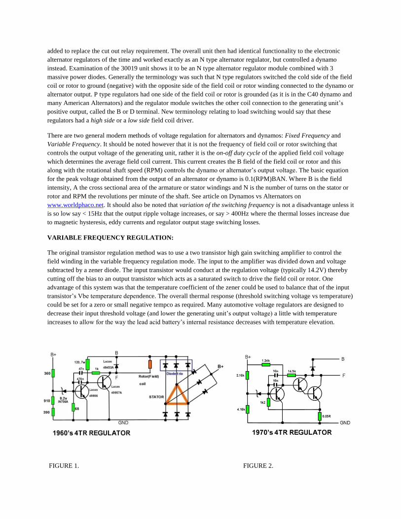
FIGURE 1. FIGURE 2.

It is worth looking at figures 1 and 2 above. Both are different, but they are of the same Alternator regulator part

number, the Lucas 4TR. They come in 3 and 4 terminal versions. One is a mid 1960’s manufacture, the other 1970’s

where they had gone to thick film technology and eliminated the high power bias resistor of their first design.

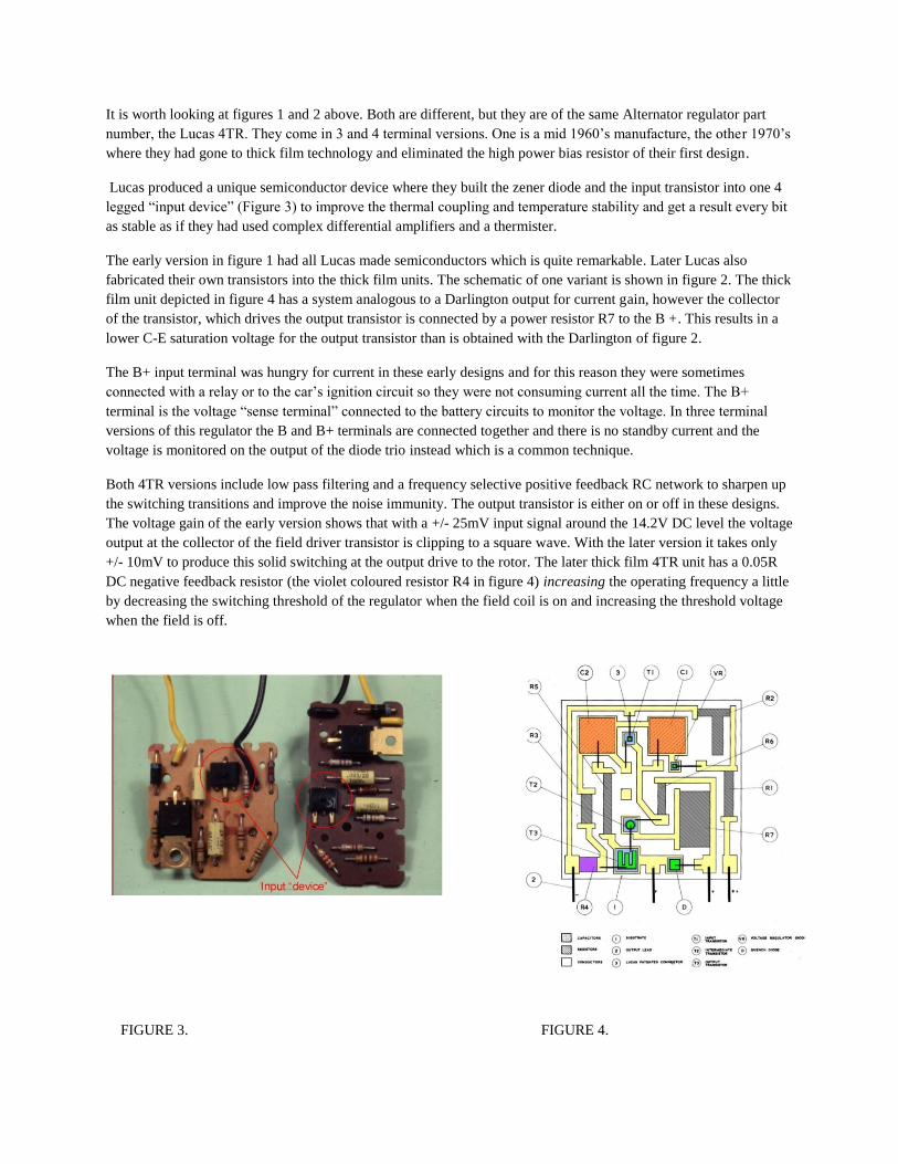
Lucas produced a unique semiconductor device where they built the zener diode and the input transistor into one 4

legged “input device” (Figure 3) to improve the thermal coupling and temperature stability and get a result every bit

as stable as if they had used complex differential amplifiers and a thermister.

The early version in figure 1 had all Lucas made semiconductors which is quite remarkable. Later Lucas also

fabricated their own transistors into the thick film units. The schematic of one variant is shown in figure 2. The thick

film unit depicted in figure 4 has a system analogous to a Darlington output for current gain, however the collector

of the transistor, which drives the output transistor is connected by a power resistor R7 to the B +. This results in a

lower C-E saturation voltage for the output transistor than is obtained with the Darlington of figure 2.

The B+ input terminal was hungry for current in these early designs and for this reason they were sometimes

connected with a relay or to the car’s ignition circuit so they were not consuming current all the time. The B+

terminal is the voltage “sense terminal” connected to the battery circuits to monitor the voltage. In three terminal

versions of this regulator the B and B+ terminals are connected together and there is no standby current and the

voltage is monitored on the output of the diode trio instead which is a common technique.

Both 4TR versions include low pass filtering and a frequency selective positive feedback RC network to sharpen up

the switching transitions and improve the noise immunity. The output transistor is either on or off in these designs.

The voltage gain of the early version shows that with a +/- 25mV input signal around the 14.2V DC level the voltage

output at the collector of the field driver transistor is clipping to a square wave. With the later version it takes only

+/- 10mV to produce this solid switching at the output drive to the rotor. The later thick film 4TR unit has a 0.05R

DC negative feedback resistor (the violet coloured resistor R4 in figure 4) increasing the operating frequency a little

by decreasing the switching threshold of the regulator when the field coil is on and increasing the threshold voltage

when the field is off.

FIGURE 3. FIGURE 4.

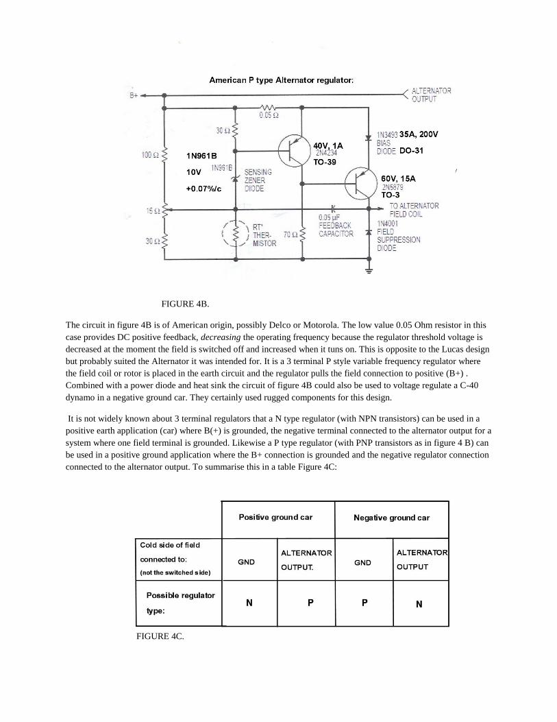
FIGURE 4B.

The circuit in figure 4B is of American origin, possibly Delco or Motorola. The low value 0.05 Ohm resistor in this

case provides DC positive feedback, decreasing the operating frequency because the regulator threshold voltage is

decreased at the moment the field is switched off and increased when it tuns on. This is opposite to the Lucas design

but probably suited the Alternator it was intended for. It is a 3 terminal P style variable frequency regulator where

the field coil or rotor is placed in the earth circuit and the regulator pulls the field connection to positive (B+) .

Combined with a power diode and heat sink the circuit of figure 4B could also be used to voltage regulate a C-40

dynamo in a negative ground car. They certainly used rugged components for this design.

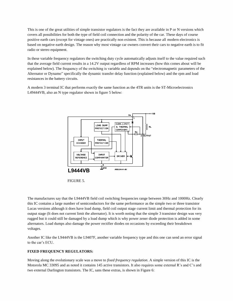
It is not widely known about 3 terminal regulators that a N type regulator (with NPN transistors) can be used in a

positive earth application (car) where B(+) is grounded, the negative terminal connected to the alternator output for a

system where one field terminal is grounded. Likewise a P type regulator (with PNP transistors as in figure 4 B) can

be used in a positive ground application where the B+ connection is grounded and the negative regulator connection

connected to the alternator output. To summarise this in a table Figure 4C:

FIGURE 4C.

This is one of the great utilities of simple transistor regulators is the fact they are available in P or N versions which

covers all possibilities for both the type of field coil connection and the polarity of the car. These days of course

positive earth cars (except for vintage ones) are practically non existent. This is because all modern electronics is

based on negative earth design. The reason why most vintage car owners convert their cars to negative earth is to fit

radio or stereo equipment.

In these variable frequency regulators the switching duty cycle automatically adjusts itself to the value required such

that the average field current results in a 14.2V output regardless of RPM increases (how this comes about will be

explained below). The frequency of the switching is variable and depends on the “electromagnetic parameters of the

Alternator or Dynamo” specifically the dynamic transfer delay function (explained below) and the rpm and load

resistances in the battery circuits.

A modern 3 terminal IC that performs exactly the same function as the 4TR units is the ST-Microelectronics

L49444VB, also an N type regulator shown in figure 5 below:

FIGURE 5.

The manufactures say that the L9444VB field coil switching frequencies range between 30Hz and 1000Hz. Clearly

this IC contains a large number of semiconductors for the same performance as the simple two or three transistor

Lucas versions although it does have load dump, field coil output stage current limit and thermal protection for its

output stage (It does not current limit the alternator). It is worth noting that the simple 3 transistor design was very

rugged but it could still be damaged by a load dump which is why power zener diode protection is added in some

alternators. Load dumps also damage the power rectifier diodes on occasions by exceeding their breakdown

voltages.

Another IC like the L9444VB is the L9407F, another variable frequency type and this one can send an error signal

to the car’s ECU.

FIXED FREQUENCY REGULATORS:

Moving along the evolutionary scale was a move to fixed frequency regulation. A simple version of this IC is the

Motorola MC 33095 and as noted it contains 145 active transistors. It also requires some external R’s and C’s and

two external Darlington transistors. The IC, sans these extras, is shown in Figure 6:

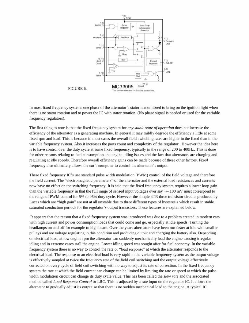
FIGURE 6.

In most fixed frequency systems one phase of the alternator’s stator is monitored to bring on the ignition light when

there is no stator rotation and to power the IC with stator rotation. (No phase signal is needed or used for the variable

frequency regulators).

The first thing to note is that the fixed frequency system for any stable state of operation does not increase the

efficiency of the alternator as a generating machine. In general it may mildly degrade the efficiency a little at some

fixed rpm and load. This is because in most cases the overall field switching rates are higher in the fixed than in the

variable frequency system. Also it increases the parts count and complexity of the regulator. However the idea here

is to have control over the duty cycle at some fixed frequency, typically in the range of 200 to 400Hz. This is done

for other reasons relating to fuel consumption and engine idling issues and the fact that alternators are charging and

regulating at idle speeds. Therefore overall efficiency gains can be made because of these other factors. Fixed

frequency also ultimately allows the car’s computer to control the alternator’s output.

These fixed frequency IC’s use standard pulse width modulation (PWM) control of the field voltage and therefore

the field current. The “electromagnetic parameters” of the alternator and the external load resistances and currents

now have no effect on the switching frequency. It is said that the fixed frequency system requires a lower loop gain

than the variable frequency in that the full range of sensed input voltages over say +/- 100 mV must correspond to

the range of PWM control for 5% to 95% duty cycle. However the simple 4TR three transistor circuits produced by

Lucas which are “high gain” are not at all unstable due to three different types of hysteresis which result in stable

saturated conduction periods for the regulator’s output transistors. These features are explained below.

It appears that the reason that a fixed frequency system was introduced was due to a problem created in modern cars

with high current and power consumption loads that could come and go, especially at idle speeds. Turning the

headlamps on and off for example to high beam. Over the years alternators have been run faster at idle with smaller

pulleys and are voltage regulating in this condition and producing output and charging the battery also. Depending

on electrical load, at low engine rpm the alternator can suddenly mechanically load the engine causing irregular

idling and in extreme cases stall the engine. Lower idling speed was sought after for fuel economy. In the variable

frequency system there is no way to control the rate or “load response” at which the alternator responds to the

electrical load. The response to an electrical load is very rapid in the variable frequency system as the output voltage

is effectively sampled at twice the frequency rate of the field coil switching and the output voltage effectively

corrected on every cycle of field coil switching with no way to adjust its rate of correction. In the fixed frequency

system the rate at which the field current can change can be limited by limiting the rate or speed at which the pulse

width modulation circuit can change its duty cycle value. This has been called the slew rate and the associated

method called Load Response Control or LRC. This is adjusted by a rate input on the regulator IC. It allows the

alternator to gradually adjust its output so that there is no sudden mechanical load to the engine. A typical IC,

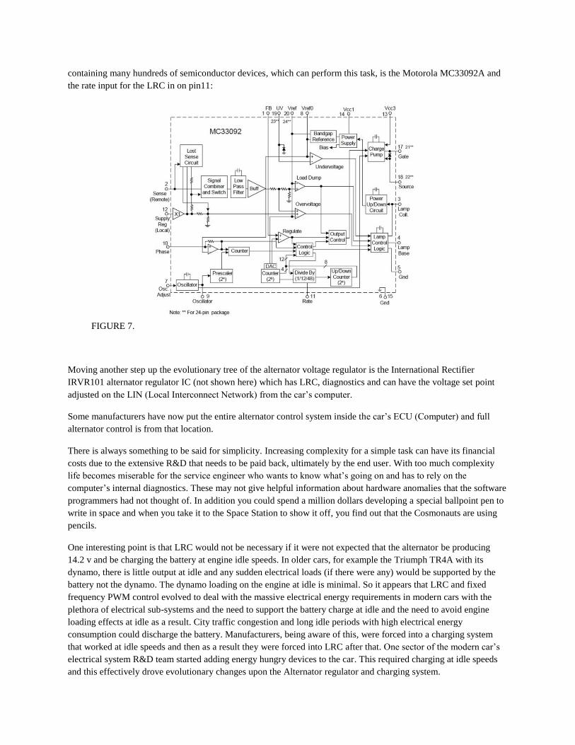
containing many hundreds of semiconductor devices, which can perform this task, is the Motorola MC33092A and

the rate input for the LRC in on pin11:

FIGURE 7.

Moving another step up the evolutionary tree of the alternator voltage regulator is the International Rectifier

IRVR101 alternator regulator IC (not shown here) which has LRC, diagnostics and can have the voltage set point

adjusted on the LIN (Local Interconnect Network) from the car’s computer.

Some manufacturers have now put the entire alternator control system inside the car’s ECU (Computer) and full

alternator control is from that location.

There is always something to be said for simplicity. Increasing complexity for a simple task can have its financial

costs due to the extensive R&D that needs to be paid back, ultimately by the end user. With too much complexity

life becomes miserable for the service engineer who wants to know what’s going on and has to rely on the

computer’s internal diagnostics. These may not give helpful information about hardware anomalies that the software

programmers had not thought of. In addition you could spend a million dollars developing a special ballpoint pen to

write in space and when you take it to the Space Station to show it off, you find out that the Cosmonauts are using

pencils.

One interesting point is that LRC would not be necessary if it were not expected that the alternator be producing

14.2 v and be charging the battery at engine idle speeds. In older cars, for example the Triumph TR4A with its

dynamo, there is little output at idle and any sudden electrical loads (if there were any) would be supported by the

battery not the dynamo. The dynamo loading on the engine at idle is minimal. So it appears that LRC and fixed

frequency PWM control evolved to deal with the massive electrical energy requirements in modern cars with the

plethora of electrical sub-systems and the need to support the battery charge at idle and the need to avoid engine

loading effects at idle as a result. City traffic congestion and long idle periods with high electrical energy

consumption could discharge the battery. Manufacturers, being aware of this, were forced into a charging system

that worked at idle speeds and then as a result they were forced into LRC after that. One sector of the modern car’s

electrical system R&D team started adding energy hungry devices to the car. This required charging at idle speeds

and this effectively drove evolutionary changes upon the Alternator regulator and charging system.

The transduction of fuel to mechanical energy by the engine is approximately 40% efficient and the alternator (or

dynamo) 60% efficient in the transfer mechanical to electrical energy, making the overall efficiency of the

transduction from petrol to electrical power about 24% efficient. As pointed out in my other articles this makes the

small cars from yesteryear with low electrical energy requirements more efficient than their new vehicle

counterparts despite the hype of energy efficient components like “more efficient alternators” in modern cars for

example. In the early car designs, mechanical power, taken directly from the engine, powers the carburation (fuel

delivery), the fuel pump and the radiator fan. Most of which are electrically powered in the modern vehicle. This

also makes the simple two and three transistor voltage regulators look very clever, very elegant and very efficient

compared to the complex IC’s with hundreds of semiconductors needed for LRC.

In general, for any given rotor or field coil power demand, the regulator (simple variable frequency or complex fixed

frequency) is not the major determinant of the voltage regulator induced ripple in the dynamo or alternator regulated

output, but rather the internal resistance properties of the dynamo or alternator and the load resistances to the battery

determine the ripple voltage due to voltage regulator activity. In the alternator there is also the 3 phase ripple of the

three phase rectification process and this can be quite significant under high alternator loads and inject audio

frequency whine into the car’s electrical system. Ripple from commutation in the dynamo system is fairly minor and

usually not problematic.

VARIABLE FREQUENCY REGULATOR STABILITY AND SWITCHING BEHAVIOUR:

Electrical Hysteresis type 1:

This is best illustrated by an equivalent circuit of a generator with the system resistances in figure 8 below. In my

dynamo test machine the wiring resistance Rw between the dynamo output and the battery has a resistance of about

0.04 Ohms. The small lead acid battery in the unit has internal resistance Rb of about 0.05 Ohms. (A typical car

sized battery is around 0.015 Ohms) The battery in the circuit below has a voltage represented by Vb and the

generating unit a voltage represented by Vg. The generating unit has an internal resistance Rg which is around 0.5

Ohms for the C40 dynamo. During charging the forward biased power rectifier has an effective resistance of around

0.01 Ohms over the range of currents from 1 to 30 A. The combination of resistances comprising Rb, Rw, Rd and

Rg results in an effective resistance Rt (the Thevenin resistance) that the voltage regulator sources field current

from. There is a voltage drop or voltage increase, due to Rt, with field coil switching on and off respectively. For

example with the field coil switching on and off, powered by the D (or B) terminal, with an average current of Q

amps, the switching transitions result in a voltage transient on the B or supply voltage equal to Q. Rt volts.

FIGURE 8.

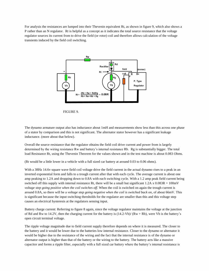
For analysis the resistances are lumped into their Thevenin equivalent Rt, as shown in figure 9, which also shows a

P rather than an N regulator. Rt is helpful as a concept as it indicates the total source resistance that the voltage

regulator sources its current from to drive the field (or rotor) coil and therefore allows calculation of the voltage

transients induced by the field coil switching.

FIGURE 9.

The dynamo armature output also has inductance about 1mH and measurements show less than this across one phase

of a stator by comparison and this is not significant. The alternator stator however has a significant leakage

inductance. (more about that below).

Overall the source resistance that the regulator obtains the field coil drive current and power from is largely

determined by the wiring resistance Rw and battery’s internal resistance Rb. Rg is substantially bigger. The total

load Resistance Rt, using the Thevenin Theorem for the values shown and in the test machine is about 0.083 Ohms.

(Rt would be a little lower in a vehicle with a full sized car battery at around 0.03 to 0.06 ohms).

With a 38Hz 14.6v square wave field coil voltage drive the field current in the actual dynamo rises to a peak in an

inverted exponential form and falls to a trough current after that with each cycle. The average current is about one

amp peaking to 1.2A and dropping down to 0.8A with each switching cycle. With a 1.2 amp peak field current being

switched off this supply with internal resistance Rt, there will be a small but significant 1.2A x 0.083R = 100mV

voltage step going positive when the coil switches off. When the coil is switched on again the trough current is

around 0.8A, so there will be a voltage step going negative when the coil is switched back on, of about 66mV. This

is significant because the input switching thresholds for the regulator are smaller than this and this voltage step

causes an electrical hysteresis at the regulators sensing input.

Battery charge current: Referring to figure 8 again, since the voltage regulator maintains the voltage at the junction

of Rd and Rw to 14.2V, then the charging current for the battery is (14.2-Vb)/ (Rw + Rb), were Vb is the battery’s

open circuit terminal voltage.

The ripple voltage magnitude due to field current supply therefore depends on where it is measured. The closer to

the battery and it would be lower due to the batteries low internal resistance. Closer to the dynamo or alternator it

would be higher due to the resistance of the wiring and the fact that the internal resistance is of the dynamo or

alternator output is higher than that of the battery or the wiring to the battery. The battery acts like a massive

capacitor and forms a ripple filter, especially with a full sized car battery where the battery’s internal resistance is

very low in the order of 0.015 Ohms rather than the 0.05 Ohms of the smaller motorcycle sized battery’s used in the

dynamo test machine.

Also when the power for the regulator module and the field coil is sourced via the diode trio in the alternator output

the source resistance at this point is a little higher due to the forward resistance properties of the smaller diodes of

the trio and the regulator induced ripple voltage here may be higher than when the regulator drives the field coil

directly from the battery circuit. So if the voltage is sensed from the diode trio also, as it often is, the running

frequency of regulator will be lower (increased Rt lowers the regulator’s running frequency- see below).

Summary of Rt:

As a result of the value of Rt, when the regulator output stage driving the field coil or rotor switches off the ripple

voltage jumps up by a value of Ipk.Rt where Ipk is the peak value of the climbing field current at the moment the

regulator switches off the field coil. Likewise when the regulator turns on and sinks current so the voltage transiently

drops down by Itr.Rt where Itr is the value that the field current had dropped down to prior to the regulator turning

the field coil back on again . Itr is less than Ipk so the negative going voltage spike of the regulator induced ripple

voltage is a little lower in amplitude than the positive going one (this will be seen in recordings below).

This common source resistance Rt means that with each on-off switching event of the regulator that the voltage that

the regulator is monitoring is altered by its own activity. This causes the regulator system to have electrical

hysteresis (called type 1 in this article) and helps the regulator to remain latched in one state until the output voltage

slopes back to the regulator’s threshold voltage. In addition there is another source of electrical hysteresis (type 2)

that encourages this behaviour too.

It should also be noted that the amplitude of the ripple voltage due to voltage regulator function is the same whether

or not the type of regulator is a variable frequency or a fixed frequency type as it relates to the field coil current

being taken from the supply for the on time of the switching cycle and not for the off time. During the off time the

field current still flows within he field coil and snubber diode circuit (not the regulator and battery circuit) and is

stabilised by the snubber diode across the field coil such that the rise of field current during the on time is similar to

the decay of field current in the off time. Higher frequency operation, typical in the fixed frequency systems results

in lower fluctuations of field coil current around the same average values, so the magnitude of the values of Ipk and

Itr tend to be more similar.

Electrical Hysteresis type 2:

One other cause of electrical hysteresis comes about as a result of the transit delay (Dt) of any signal via the standard

variable frequency regulator from its input to its output. Although this is not large for an electronic regulator, for

example 200 uS, it causes an additional electrical hysteresis. The input threshold voltage for the regulator which

corresponds to the moment that the regulator output switches is higher than 14.2V for a positive going input voltage

and lower than 14.2 volts for a negative going voltage input. Both causes of electrical hysteresis type 1 and 2 results

in the regulator adopting a stable switched on or off state while the dynamo or alternator output more gradually

changes its output voltage in response to the field current rising and falling as a result. Evaluating a simple two or

three transistor switching regulator shows that when the unit is driven by a square wave input there is a delay Dt

before the regulator output changes state. This delay relates to the time it takes for the output transistor to pass in

and out of saturation and due to the effect of the filter capacitor (integrator capacitor) from the collector to the base

of the input transistor. This is summarised in the diagram below Figure 10:

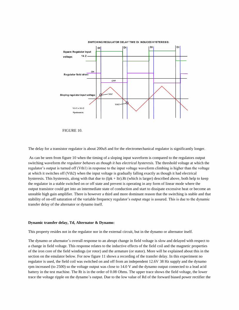
FIGURE 10.

The delay for a transistor regulator is about 200uS and for the electromechanical regulator is significantly longer.

As can be seen from figure 10 when the timing of a sloping input waveform is compared to the regulators output

switching waveform the regulator behaves as though it has electrical hysteresis. The threshold voltage at which the

regulator’s output is turned off (Vth1) in response to the input voltage waveform climbing is higher than the voltage

at which it switches off (Vth2) when the input voltage is gradually falling exactly as though it had electrical

hysteresis. This hysteresis, along with that due to (Ipk + Itr).Rt (which is larger) described above, both help to keep

the regulator in a stable switched on or off state and prevent is operating in any form of linear mode where the

output transistor could get into an intermediate state of conduction and start to dissipate excessive heat or become an

unstable high gain amplifier. There is however a third and more dominant reason that the switching is stable and that

stability of on-off saturation of the variable frequency regulator’s output stage is assured. This is due to the dynamic

transfer delay of the alternator or dynamo itself.

Dynamic transfer delay, Td, Alternator & Dynamo:

This property resides not in the regulator nor in the external circuit, but in the dynamo or alternator itself.

The dynamo or alternator’s overall response to an abrupt change in field voltage is slow and delayed with respect to

a change in field voltage. This response relates to the inductive effects of the field coil and the magnetic properties

of the iron core of the field windings (or rotor) and the armature (or stator). More will be explained about this in the

section on the emulator below. For now figure 11 shows a recording of the transfer delay. In this experiment no

regulator is used, the field coil was switched on and off from an independent 12.6V 38 Hz supply and the dynamo

rpm increased (to 2500) so the voltage output was close to 14.0 V and the dynamo output connected to a lead acid

battery in the test machine. The Rt is in the order of 0.08 Ohms. The upper trace shows the field voltage, the lower

trace the voltage ripple on the dynamo’s output. Due to the low value of Rd of the forward biased power rectifier the

ripple looks the practically same on both sides of the power rectifier and shorting the rectifier has little observable

effect.

Of note is the smaller commutator ripple appearing as sinusoidal like modulation superimposed on the main ripple

voltage output. The main 100mV pp ripple output is due to fluctuations in the field coil current and the magnetic

field values of the iron core of the field coil and that of the armature. Notice how the voltage is delayed with respect

to the field voltage (it is also delayed with respect to the current too). The point to note is that immediately after the

field coil is switched off, the output voltage keeps climbing for a while before turning around and beginning to fall.

Ignoring the finer commutator ripple the basic output ripple voltage waveform has been drawn over in red.

FIGURE 11.

Therefore, in the case where the voltage regulator output stage is driving the field coil after it switches the field coil

on or off, the field coil (or rotor) inductance delay and combined iron core magnetic hysteresis delays of the dynamo

itself results in the regulator’s output state remaining stable for a time until the voltage turns around and heads off

toward the voltage regulator’s switching threshold value. Putting the two electrical hysteresis properties and the

transfer delay property together in one diagram to summarise the regulator and dynamo activity while the regulator

is in control, and in usual use, figure 12:

FIGURE 12

Therefore the voltage regulator’s input voltage or hysteresis voltage range is at total of Vth1-Vth2 + Rt(Ipk + Itr).

On an actual recording these features are easy to see, along with the additional small commutator ripples. See figure

13. (In the alternator these would be represented by three phase rectification ripples).

FIGURE 13.

Notice that Itr.Rt is a little lower than Ipk.Rt as expected. It is now easy to see then why the simple two or three

transistor variable frequency regulators end up self oscillating when configured with a dynamo or alternator.

Although the circuit of the N type regulator may not look like it is an inverting amplifier, it still is because as its

input voltage climbs the field coil is turned off just as it is in a P type regulator.

We have a high gain inverting amplifier (the regulator) with hysteresis at its input created by both Dt and the

common resistance Rt that the regulator is both switching across and voltage sensing. Then we have a delay

function, Td, from its input to its output (the alternator or dynamo itself). This creates an oscillator circuit very

familiar to every electronics engineer where the input voltage oscillates around two input threshold voltages and the

output, just like the output of the regulator module, behaves as a saturated switch. Td is formed by an RC network in

this analogy, see figure 14:

FIGURE 14:

The information above explains why self oscillation of the variable frequency regulators is a stable phenomenon due

to the transfer delay and the hysteresis.

The information above also applies to fixed frequency regulators too, in that the basic ripple induced by switching

regulation on the output voltage will still be Rt(Ipk+Itr) which is the largest component of the ripple voltage along

with the dynamo or alternator’s transfer delay. Ipk and Itr will have a close value at the higher frequencies, say

400Hz of a fixed frequency system and tend to approach the average field current value.

The phase delay in the actual dynamo system is a little longer than the delay provided by the RC network analogy of

figure 14 but system oscillations are still guaranteed.

Vth1 and Vth2 will not exist in the fixed frequency regulator system as the filtering is such that the PWM control of

the fixed frequency system can only make slow changes in duty cycle and average field currents and does not have a

delay time Dt characteristic that operates twice per switching cycle of the field or rotor coil which induces the Vth1

and Vth2 ripple component in the variable frequency system.

Summary of Dt, Vth 1 & 2 and Rt and the dynamic transfer delay Tda, Tdp andTds:

An increase in Vth1 and Vth2 or an increase in Rt both result in an increases peak to peak ripple voltage. This

increases the electrical hysteresis margin that is operating at the voltage regulator’s input and as a result lowers the

operating frequency for the variable frequency regulator. Substituting an electromechanical regulator, with a much

larger Dt increases Vth1 and Vth2 and results in a lower operating frequency. Adding electrical filtering within an

electronic regulator increases Vth1 and Vth2 and therefore lowers the operating frequency and increases the ripple

voltage for two reasons, firstly Vth1 and Vth2 are larger, also Ipk and Itr are higher in magnitude at a lower field

coil frequency.

The transfer delay Td is a property of the dynamo or alternator model itself relating to its inductance and the

magnetic hysteresis properties of the iron cores of the field coil (rotor) and armature (stator). It can be broken into 3

parts: Tda or the amplitude of the output ripple, Tdp or the phase of the transferred field ripple with respect to the

field voltage and Tds or the shape of the overall output ripple all at some rpm value. This can be easily measured

with an independent field (or rotor) coil drive system and a dual channel oscilloscope from a rotating unit. Then a

suitable filter module constructed to match these properties as closely as possible.

It is now worth noting some interesting points:

Any alternator or dynamo emulator used to test a fixed frequency regulator does not have to be very precise in its

design. It does not need to match up with Tda, Tdp or the Tds of the unit being emulated and also Rt won’t affect the

operating frequency. However for testing the common variable frequency regulators the three Td parameters must

be very close and the Rt value about what it would be in the vehicle, or the regulator being tested will not run at the

actual frequency it would in the vehicle. Not that the running frequency value is too critical in terms of voltage

regulation but it is best to have the emulator match the real rotating machine as closely as possible.

When designing or testing simple transistor variable frequency regulators:

1) Increasing the low pass filtering within or at the input of the regulator circuitry increases Dt and therefore

increases the difference between VTh1 and Vth2 and lowers the operating frequency and also increases the regulator

induced ripple voltages because Ipk and Itr also increase at lower running frequencies.

2) DC negative feedback within the regulator modifies Vth1 and Vth2. This was done in the Lucas 1970’s 4TR

regulator figure 2. It increases the operating frequency and synthetically opposes the effects of Rt or the common

impedance from which the regulator unit both draws current to supply the field coil.

3) DC positive feedback, as done within the American alternator regulator figure 4B lowers the operating frequency.

4) The electronic regulator itself: Unless the filtering and delay within it is excessive, is not the determinant of the

operating frequency. The primary determinant is the electromagnetic properties of the alternator or dynamo with the

dynamic transfer delay Td, in conjunction with the low ohmic resistances of the battery charging circuit combined

with the internal resistance of the dynamo or alternator, the effective equivalent resistance being Rt, or the Thevenin

equivalent. Rt and the transfer delay Td are independent of the regulator unit.

5) Electromechanical regulators behave exactly as an electronic regulator with heavy filtering due to the magnetic

hysteresis of the voltage regulator relay coil core and some combined inertia due to the mass of the moving parts.

Therefore electro-mechanical regulators run the system at a lower frequency (around 25Hz) compared to an

electronic regulator (around 50Hz) for the C40 dynamo and RB106 system for example.

6) Even without the two forms of electrical hysteresis of Ipk.Rt, Itr.Rt and Vth1 and Vth2, the system with the

typical variable frequency voltage regulator would still be oscillatory, but at a higher frequency. This is due to Td

alone. As can be seen from the recordings at the moment the field coil switches off at some voltage regulator input

threshold voltage, the dynamo output continues to rise for a time before falling again. This phase delay alone would

induce stable switched on or off states in the regulator unit’s output stage. Running with zero electrical hysteresis

(Vth1 = Vth2 and Rt =0) the system will oscillate at a higher frequency where the phase delay of Td is around 180

degrees which results in net positive feedback ensuring oscillations. The two forms of electrical hysteresis cited

above simply have the effect of lowering the switching frequency. In use the frequency stabilises at some values

related to the transfer delay and the electrical hysteresis. However it is the duty cycle of the field coil drive and the

average field coil current, not the switching frequency, which determines the output voltage of the dynamo or

alternator.

7) A dynamo or alternator Emulator must not only emulate the transfer delay and other electrical properties of the

particular charging machine, but also the properties of the battery circuit and wiring, otherwise Rt will not be similar

and the regulator under test will not behave as it would in actual use in the vehicle.

8) In the practical emulator (described below) the dummy field coil inductance does not have a core with identical

magnetic properties to the actual dynamo field or rotor core, so that the peaks and troughs of current Ipk and Itr are a

little higher. This can be compensated for by lowering Rg and therefore Rt, so to keep Ipk.Rt and Itr.Rt similar

between the actual dynamo and the emulator.

9) If one is designing a fixed frequency regulator, it is important that the loop gain is not too high. The full range of

PWM say 5% to 95 % duty cycle should be created by a sensed ripple voltage of about +/- 100mV. If it was say

10mV, then the system will instead behave as a variable frequency system where the PWM controller simply flips

between 5% and 95% duty and the extra switching events between these slower duty cycle flips from the PWM IC

simply degrade the efficiency.

Now that the voltage regulators have been discussed and the dynamo’s or alternator’s dynamic transfer delay Td

has been alluded to, we can move on to describe the Emulator and the required properties so that the voltage

regulator can be tested and a hardware version of the emulator can be made or a Spice version drawn up.

********************************************************************************************

REQUIREMENTS OF A DYNAMO & ALTERNATOR EMULATOR:

There are a number of major and minor features of the alternator or generator being emulated, these are:

Major:

1) Average transfer characteristic:

(Average field coil current and RPM vs B field levels and output voltages).

2) Output resistance Rg and Thevenin equivalent Rt when loaded to the vehicle’s charging system.

3) Dynamic transfer delay Td and the three properties of it: Tda, Tdp and Tds.

(Relationship between applied alternating field coil voltage and field coil current vs B field levels and output

voltages, field inductance integration and B-H curve filtering & magnetic hysteresis of the cores).

4) Power output capability.

Minor:

5) Regulation: Effect of Armature reaction (dynamo) or Stator reaction Alternator.

6) Losses due to: Magnetic Hysteresis, eddy currents, copper losses & frictional losses and windage.

7) Commutator ripple & spikes (dynamo) or 3 phase ripple (alternator whine) and regulator switching transient

whine (interference).

8) Phase signal for alternator regulators with a phase input.

For the application of creating an Emulator for testing voltage (and current regulator if present) the first 4 features

are the essential ones. The other minor features can be added to the emulator later as required. No significant current

loading or power output capability is needed to check the typical alternator voltage regulator functionality as they

don’t detect current levels, only voltage.

THE MINOR FEATURES FIRST:

Regulation:

Armature reaction is the effect that armature current and therefore the armature’s magnetization has on the B field of

the field coils in the dynamo. This drags the B field around a little in the direction of rotation and weakens the B

field a little. At high load currents this is one of the reasons that the dynamo’s voltage drops off, along with the

resistance of the armature windings and brushes. Mechanical rectification is quite unique in that the resultant emf or

output from the dynamo can be looked upon as due to the same number of armature coil turns (but not the same

actual turns) occupying the same place or position within the B field. To see how the C40 armature and commutator

works see article on www.wolrdphaco.net The regulation is such that when the dynamo is loaded, the voltage output

drops down because of the DC resistance of the armature windings, commutator and brushes and the armature

reaction.

The factors which affect the regulation of the Alternator are a little more involved. In the alternator the output

current via the stator and the magnetic effects of this is also called “armature reaction”. In essence here, just as it

does in a synchronous motor, a magnetic flux wave due to the ampere-turns of the stator moves around at

synchronous speed and alters the total flux of the magnetic poles of the rotor. The Ampere-turn induced flux wave

from the stator current is very close to a sine wave in shape. Its exact position, or phase, with respect to the rotating

B field of the rotor varies with the power factor of the load. This is the phase relationship between output voltage

and output current. When the output voltage is in phase with the current (power factor =1) the effect is a distortion

of the rotating B field of the rotor. However the AC Stator current also results in a leakage reactance which makes

the stator windings appear more inductive. This inductance causes a drop in the power factor below unity (even if

the alternator’s load is purely resistive) with the output current lagging behind the voltage and this results in

demagnetisation of the poles. With a zero power factor for example (output current lagging 90 degrees behind the

output voltage) the stator’s Ampere-turn flux wave has shifted to a position where is completely opposes that of the

rotating B field of the rotor, so the B field is significantly weakened. Therefore, for the alternator with a constant

field (rotor)current, the voltage output drops with loading because of the decrease in flux per pole due to armature

reaction (just like a dynamo) and the impedance (inductance and resistance) of the stator winding. This is unlike the

dynamo case where only the resistance and not the impedance is the important feature.

In the closed loop system with the voltage regulator operating within its dynamic control range all of the above

causes for voltage drop, at the point where the regulator’s sensing connection is connected, are compensated for and

the output voltage is stable with the ripple voltages of close to (Vth1 + Ipk.Rt) above and (Vth2 + Itr.Rt) below the

stable output voltage of typically 14.2V.

Hysteresis & Eddy Currents:

Magnetic hysteresis of the field coil’s core (or rotor) also causes a loss of energy proportional to the frequency of the

field coil switching. Magnetic hysteresis is a form of magnetic memory and with each cycle of magnetization and

demagnetization work is done to overcome it. In the field coil system (or rotor coil) the average current is DC and

the AC component fluctuates over a smaller range thus reducing the hysteresis losses. The range of core

magnetisations runs along the upper part of the field coil’s B-H curve (discussed below) this significantly reduces

the hysteresis losses here because the area inside the hysteresis loop is very small.

Similar hysteresis loss principles apply to the iron core of the armature or stator. They experiences full B field flux

reversals as the armature rotates in the B field in the dynamo or the B field poles of the rotor rotate inside the stator

of the alternator. A complete flux cycle occurs in the dynamo once per shaft revolution. Depending on the design of

the Alternator (usually 3 pole pairs) there are 3 complete flux cycles per rotation. The alternator shaft speeds could

be twice that of the dynamo due to the smaller pulleys, so one could say the hysteresis losses in the 3 pole alternator

could be 5 or 6 times that of the comparable 1 pole dynamo.

Eddy currents circulating in the magnetic core also dissipate energy in proportion to the square of the frequency.

This is why many iron cores are laminated with varnish between the strips of metal. Eddy current losses in the stator

of the alternator could be expected to be 25 to 36 times higher than that in the dynamo’s armature.

Frictional Losses:

Bearing friction and fan resistance and coil resistances waste input energy and there is significant energy dissipation

by the rectifier packs in Alternators at high current loads. The forward voltage drops of silicon power rectifiers, at

high currents, are generally around 0.8 volts and at any one moment two are always conducting in full wave

rectification. So with a 40 amp output the power loss is around 40 x 1.6 = 64 watts and the rectifier pack is hot,

assisted by fan cooling. Low voltage drop Schottky rectifiers can help here, however most manufactures have stuck

with standard silicon power rectifiers as they have higher reverse voltage ratings than the Schottkys and are less

prone to be damaged by load dumps, they also generally have a lower reverse leakage current too. Electrical

resistance (copper losses) in the stator and armature drops voltage with current, wasting energy as heat.

Ripple & Whine:

Commutator ripple and spikes appear in a dynamo’s voltage output. Ripple from the 3 phase AC current passing via

the rectifier pack in the alternator also appears on the output voltage. (Also ripple from the switching function of the

regulator appears at the unit’s output- this is part of a major feature). In all cases these smaller “signals” arise from a

very low source resistance and can be very difficult to filter out. Sometimes they cause annoying audio frequency

interference, often due to currents in common earth pathways in cars or aeroplanes. The alternator is more

troublesome than the dynamo in this respect as the frequency of the stator ripple is in the audio range and can have

significant amplitude when the alternator’s current output is high. Signals to replicate these can be injected into the

input of the power amplifier of the Emulator if required. A failed diode in a rectifier pack in the alternator

unbalances the 3 phase currents and this can result in significant alternator whine to audio apparatus in the vehicle.

Phase signals:

Simple two or three transistor variable frequency regulators do not require any form of phase signal input to operate.

For the more complex regulator IC’s they often use the phase signal, taken from one stator winding for various

applications. One is to power the IC when alternator rotation is detected another is to turn on the warning lamp when

the alternator stops. Also the signal can be used in coordinating the LRC system or in error messages to the

ECU(computer).

A phase signal can be added to an emulator as a “pulse waveform proportional” in frequency to the position of the

RPM control on the Emulator and having a frequency equal to what the alternator being modelled would produce at

that RPM.

THE MAJOR FEATURES:

Firstly there is no difference in the alternator or dynamo in terms of electronic voltage regulator functionality.

In the case of the dynamo the stationary field winding is driven by the regulator to generate and control the B field

and the rotating armature coils cut (pass through) the B field to provide a changing magnetic flux. The changing flux

produces the output voltage in the armature coils according to Faraday’s Law of induction. This ultimately provides

the DC output from the armature with the aid of mechanical rectification (the commutator). The method of

rectification is however academic with respect to the voltage regulator’s function. In the case of the alternator the

regulator drives the rotor to create and control a rotating B field which cuts the turns of the stationary stator winding,

so it’s the same relative motion. This produces the changing magnetic flux and a 3 phase AC output voltage from the

stator. This is electronically rectified to DC by a full wave three phase rectifier (six power diodes) to yield the DC

output.

Magnetizing force H:

The magnetizing force H is developed around the field coil’s wires due to the current in the wires. The value of H

therefore depends on the number of turns of the field coil and the field current in amps and inversely to the path

length of the magnetic circuit in meters (the geometry of the iron core). The field coil current provides the

magnetizing force H for the iron core of the rotor body or field coil core. Ampere’s Law states that H = Ni/L, where

i is the current, N the number of turns or wire and L the magnetic path length. H has units of ampere-turns per meter.

The magnetic “flux density” created in the iron core, or the “magnetization” of the iron, is denoted as the B field. In

general B = μH, where μ is the permeability of the iron core material. It is not a linear relationship with an iron core

because the μ value of the core climbs with initial magnetizing force H and falls to a lower value at higher

magnetizing force as a property of the iron core. The core therefore begins to saturate at high flux densities and the

value of μ falls off. Proportional percentage increases in field current and therefore H value do not increase the value

of the B field or the voltage output of a generator to the same proportion.

In addition with a zero field current, some residual magnetization remains in the iron and there is a residual B field.

Therefore some generator output voltage occurs in proportion to the RPM as the generator is rotating with no field

coil current. This is important in initial excitation of the field coils when the unit starts to rotate. Generally most

generator units power their own field windings and rotor windings via the voltage regulator.

One could also write B = μ(H + M), where M is some amount of residual magnetism in the iron core. Also it is

worth remembering that the peak output voltage from a dynamo is directly proportional to the value of the B field

and the RPM. For a dynamo, the peak voltage output expected is 0.1 x RPM x BAN, where RPM is the revolutions

per minute of the dynamo shaft, B is the flux density of the field, A is the cross sectional area of the armature turns

and N is the number of armature turns. The emf equation of the alternator is a little more involved however the same

basic principle applies where the peak output voltage of one of the phases is directly proportional to the RPM and

the value of B.

More about the relationship between B and H:

In general because the H field is proportional to the field coil current and the output voltage of the generating unit

proportional to the B field then at some RPM, the graph of the field (or rotor) current vs generator or alternator

voltage output simply looks like the B-H curve of an iron cored inductor which represents the magnetic properties of

the sample of iron. B-H curves also exhibit the phenomenon of magnetic hysteresis due to the magnetic properties or

magnetic memory of the iron.

The term magnetic hysteresis was used to distinguish it from electrical hysteresis also discussed in this article

relating to the switching functions of simple two and three transistor regulators discussed above.

Without voltage regulation employed, the relationship between RPM of the generator’s shaft and the output voltage

off load is linear for any fixed value of B (or field current). The relationships are summarized in the diagram below

of figure 15. This is a sketch of the type of data obtainable from a Lucas C40 Dynamo tested off load.

These are standard results and are typical for any generating machine in terms of the basic features of the shape and

the effect of the residual magnetism M (residual B field) of the field core. The residual magnetism means that even

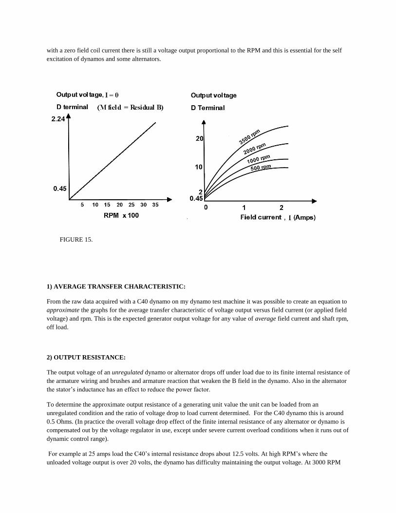
with a zero field coil current there is still a voltage output proportional to the RPM and this is essential for the self

excitation of dynamos and some alternators.

FIGURE 15.

1) AVERAGE TRANSFER CHARACTERISTIC:

From the raw data acquired with a C40 dynamo on my dynamo test machine it was possible to create an equation to

approximate the graphs for the average transfer characteristic of voltage output versus field current (or applied field

voltage) and rpm. This is the expected generator output voltage for any value of average field current and shaft rpm,

off load.

2) OUTPUT RESISTANCE:

The output voltage of an unregulated dynamo or alternator drops off under load due to its finite internal resistance of

the armature wiring and brushes and armature reaction that weaken the B field in the dynamo. Also in the alternator

the stator’s inductance has an effect to reduce the power factor.

To determine the approximate output resistance of a generating unit value the unit can be loaded from an

unregulated condition and the ratio of voltage drop to load current determined. For the C40 dynamo this is around

0.5 Ohms. (In practice the overall voltage drop effect of the finite internal resistance of any alternator or dynamo is

compensated out by the voltage regulator in use, except under severe current overload conditions when it runs out of

dynamic control range).

For example at 25 amps load the C40’s internal resistance drops about 12.5 volts. At high RPM’s where the

unloaded voltage output is over 20 volts, the dynamo has difficulty maintaining the output voltage. At 3000 RPM

and a 30A overload the C40 produces about 13V output on its D terminal and in this condition the field coil drive is

hard on to 2 amps and the voltage regulator is inactive and the voltage control is outside the system’s dynamic range

(Any incorporated current limiter would be active under these conditions and be reducing the drive to the field coils

by switching them on & off so as to stabilise the maximum output current to 22A in the case of a c40 dynamo).

As noted in figures 8 and 9 above, when the dynamo is in use with a voltage regulator and battery charging system

the source resistance seen by the voltage regulator is Rt, which is a lower value than the internal resistance Rg of the

generating unit and this is because of the lead acid battery’s low internal resistance Rb and the low resistance of the

wiring to the battery Rw.

3) DYNAMIC TRANSFER FUNCTION Td:

This is the more difficult part of the emulator. If this is not correct then testing of variable frequency systems, where

this transfer delay is responsible in part for determining the operating frequency would give abnormal results.

Obviously a dynamo or alternator emulator would have to have a similar overall transfer function as the real

machine and a similar output resistance to be of value in bench testing voltage regulator modules. The overall

dynamic transfer function wave has amplitude (Tda), phase (Tdp) and shape (Tds) characteristics. Td results from

the integration effect of the field coil (or rotor) inductance and its iron core and the armature (or stator)iron core and

needs to be replicated electronically.

For example with the C40 dynamo unregulated and a 12.6V peak to peak 50Hz square wave applied to the field coil

with a DC offset of 6.3V and an average field current of 1 amp and at 2500 RPM loaded into an equivalent Rt of

0.08 Ohms: When one examines the field coil ripple voltage (figure 11) transferred to the output (D terminal) it is

only in the order of 100mVpp or only about 0.7% of the output voltage (or peak field voltage) and has a sinusoidal

rather than square profile. The amplitude value increases or decreases along with the RPM value because the voltage

output of a generator is proportional to product of the B field value and the rpm. So the question here is: why is there

significantly less voltage fluctuation at the generator’s output than the voltage fluctuations applied to the field coil?

The answer to this question has three parts: Firstly, the field coil in a C40 has an inductance of about 45 to 50mH

and a DC resistance of 6 to 7 ohms. When square wave voltage applied to the field coil terminal this does not

generate a square wave field current, but instead an exponentially rising and falling current. The magnitude of the

fluctuations decreases with increasing frequency and the average current value depends on the duty cycle of the

driving voltage waveform. The field coil (inductance & resistance) acts as a filter or integrator for current in an

analogous manner that a low pass RC network acts as an integrator for voltage. Therefore the inductance of the field

coil core results in the percentage of the field current fluctuations (compared to the field voltage fluctuations) being

delayed and reduced in magnitude. The oscillogram below, figure 16, shows the typical relation between an applied

50Hz square wave voltage and the current for a C40 dynamo field coil. The same applies to an alternator rotor:

FIGURE 16.

However the peaks and troughs are also reduced to what they would be with a perfect 45mH inductor because of the

magnetic hysteresis of the iron core. Running the equivalent circuit in the Spice simulator (figure 17) for example

yields higher current peaks and troughs than measured with the actual iron cored field coil.

FIGURE 17.

The current peaks and troughs are significantly lowered by the presence of the iron core and its magnetic hysteresis.

This is due to the shape of the B-H curve of the field coil’s iron material and the fact that the B-H curve is running

along its upper edge because a DC bias and average magnetisation is applied.

The magnetisation force field H is proportional to the field coil current and easy to measure simply by placing a low

value resistor (0.5 ohms) in series with the field coil and measuring the voltage across it and dividing by the

resistance. To acquire the B value I made a magnetic probe with two Hall sensors in a bridge configuration and

placed one of them into a non rotating dynamo’s field area. This enabled the recordings of hysteresis loops below.

These are simply X-Y plots of field current versus the magnetic flux density of the field’s iron core, or the B value.

Figure 18 shows the hysteresis loop plot. The B field signal was gain adjusted to be approximately equal to the

deflection produced by the field current so that relative fluctuations could be compared. The H field is proportional

to the field current. This was done with a 12V field coil square wave voltage frequency of 12.5Hz and a +6V DC

offset.

FIGURE 18.

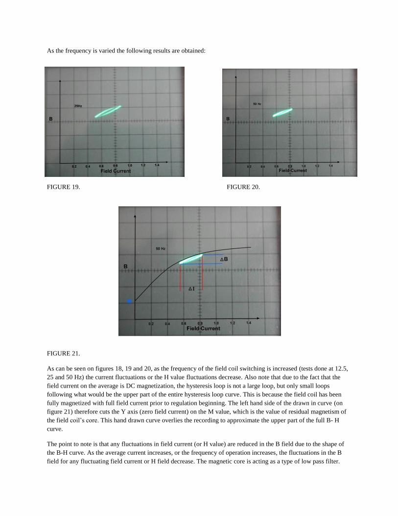
As the frequency is varied the following results are obtained:

FIGURE 19. FIGURE 20.

FIGURE 21.

As can be seen on figures 18, 19 and 20, as the frequency of the field coil switching is increased (tests done at 12.5,

25 and 50 Hz) the current fluctuations or the H value fluctuations decrease. Also note that due to the fact that the

field current on the average is DC magnetization, the hysteresis loop is not a large loop, but only small loops

following what would be the upper part of the entire hysteresis loop curve. This is because the field coil has been

fully magnetized with full field current prior to regulation beginning. The left hand side of the drawn in curve (on

figure 21) therefore cuts the Y axis (zero field current) on the M value, which is the value of residual magnetism of

the field coil’s core. This hand drawn curve overlies the recording to approximate the upper part of the full B- H

curve.

The point to note is that any fluctuations in field current (or H value) are reduced in the B field due to the shape of

the B-H curve. As the average current increases, or the frequency of operation increases, the fluctuations in the B

field for any fluctuating field current or H field decrease. The magnetic core is acting as a type of low pass filter.

This is also why iron cored transformers have a limit to their upper frequency response. The net effect is one of low

pass filtering where field coil current fluctuations are reduced in the B field. Given that the generator’s output

voltage is proportional to the B field, then the fluctuations are reduced in the generator’s output voltage. At higher

currents the core tends to saturate and the low pass filter effect is further enhanced.

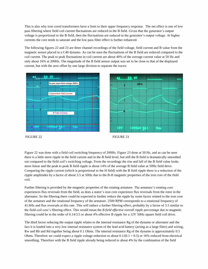
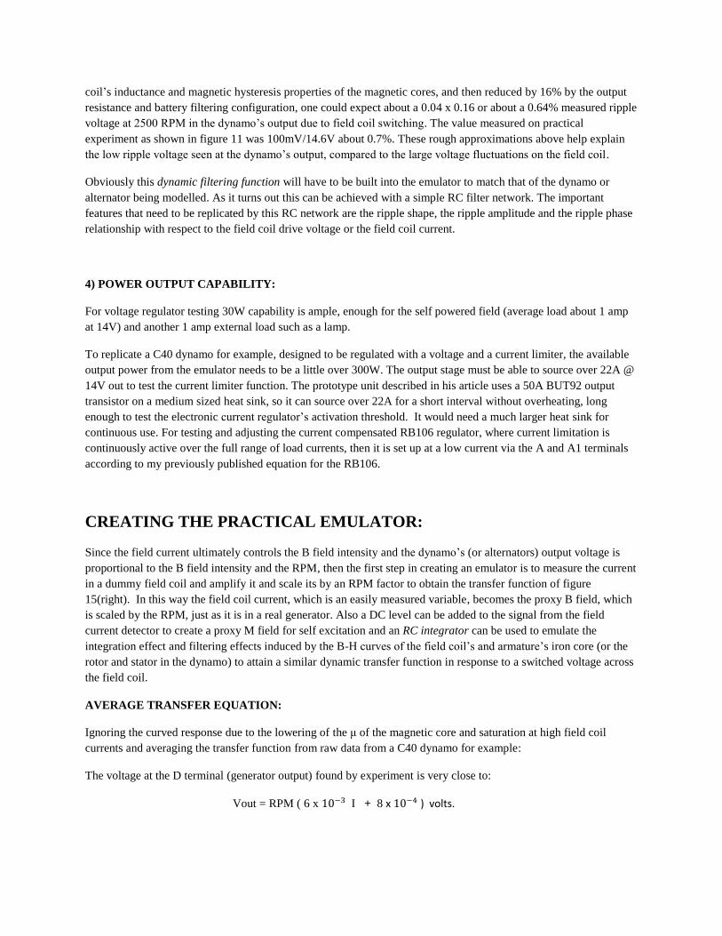
The following figures 22 and 23 are three channel recordings of the field voltage, field current and B value from the

magnetic sensor placed in a C40 dynamo. As can be seen the fluctuations of the B field are reduced compared to the

coil current. The peak to peak fluctuations in coil current are about 40% of the average current value at 50 Hz and

only about 16% at 200Hz. The magnitude of the B field sensor output was set to be close to that of the displayed

current, but with the zero offset by one large division to separate the traces:

FIGURE 22 FIGURE 23

Figure 22 was done with a field coil switching frequency of 200Hz. Figure 23 done at 50 Hz, and as can be seen

there is a little more ripple in the field current and in the B field level, but still the B field is dramatically smoothed

out compared to the field coil’s switching voltage. From the recordings the rise and fall of the B field value looks

more linear and the peak to peak B field ripple is about 14% of the average B field value at 50Hz field drive.

Comparing the ripple current (which is proportional to the H field) with the B field ripple there is a reduction of the

ripple amplitudes by a factor of about 3.5 at 50Hz due to the B-H magnetic properties of the iron core of the field

coil.

Further filtering is provided by the magnetic properties of the rotating armature. The armature’s rotating core

experiences flux reversals from the field, as does a stator’s iron core experience flux reversals from the rotor in the

alternator. So the filtering there could be expected to further reduce the ripple by some factor related to the iron core

of the armature and the rotational frequency of the armature. 2500 RPM corresponds to a rotational frequency of

41.6Hz and flux reversals at this rate. This will induce a further filtering effect, probably by a factor of 3.5 similar to

the field coil core’s filtering effect. This would mean the B field effective overall ripple percentage due to magnetic

filtering could be in the order of 0.14/3.5 or about 4% effective B ripple for a 12V 50Hz square field coil drive.

The third factor reducing the output ripple relates to the internal resistance Rg of the dynamo or alternator and the

fact it is loaded into a very low internal resistance system of the lead acid battery (acting as a large filter) and wiring,

Rw and Rb and Rd together being about 0.1 Ohms. The internal resistance Rg of the dynamo is approximately 0.5

Ohms. Therefore we could expect a ripple voltage reduction to about 0.1/(0.1 + 0.5) or 16% reduced from electrical

smoothing. Therefore with the B field ripple already being reduced to about 4% by the combination of the field

coil’s inductance and magnetic hysteresis properties of the magnetic cores, and then reduced by 16% by the output

resistance and battery filtering configuration, one could expect about a 0.04 x 0.16 or about a 0.64% measured ripple

voltage at 2500 RPM in the dynamo’s output due to field coil switching. The value measured on practical

experiment as shown in figure 11 was 100mV/14.6V about 0.7%. These rough approximations above help explain

the low ripple voltage seen at the dynamo’s output, compared to the large voltage fluctuations on the field coil.

Obviously this dynamic filtering function will have to be built into the emulator to match that of the dynamo or

alternator being modelled. As it turns out this can be achieved with a simple RC filter network. The important

features that need to be replicated by this RC network are the ripple shape, the ripple amplitude and the ripple phase

relationship with respect to the field coil drive voltage or the field coil current.

4) POWER OUTPUT CAPABILITY:

For voltage regulator testing 30W capability is ample, enough for the self powered field (average load about 1 amp

at 14V) and another 1 amp external load such as a lamp.

To replicate a C40 dynamo for example, designed to be regulated with a voltage and a current limiter, the available

output power from the emulator needs to be a little over 300W. The output stage must be able to source over 22A @

14V out to test the current limiter function. The prototype unit described in his article uses a 50A BUT92 output

transistor on a medium sized heat sink, so it can source over 22A for a short interval without overheating, long

enough to test the electronic current regulator’s activation threshold. It would need a much larger heat sink for

continuous use. For testing and adjusting the current compensated RB106 regulator, where current limitation is

continuously active over the full range of load currents, then it is set up at a low current via the A and A1 terminals

according to my previously published equation for the RB106.

CREATING THE PRACTICAL EMULATOR:

Since the field current ultimately controls the B field intensity and the dynamo’s (or alternators) output voltage is

proportional to the B field intensity and the RPM, then the first step in creating an emulator is to measure the current

in a dummy field coil and amplify it and scale its by an RPM factor to obtain the transfer function of figure

15(right). In this way the field coil current, which is an easily measured variable, becomes the proxy B field, which

is scaled by the RPM, just as it is in a real generator. Also a DC level can be added to the signal from the field

current detector to create a proxy M field for self excitation and an RC integrator can be used to emulate the

integration effect and filtering effects induced by the B-H curves of the field coil’s and armature’s iron core (or the

rotor and stator in the dynamo) to attain a similar dynamic transfer function in response to a switched voltage across

the field coil.

AVERAGE TRANSFER EQUATION:

Ignoring the curved response due to the lowering of the μ of the magnetic core and saturation at high field coil

currents and averaging the transfer function from raw data from a C40 dynamo for example:

The voltage at the D terminal (generator output) found by experiment is very close to:

Vout = RPM ( 6 x I + 8 x ) volts.

Where the RPM is the shaft revolutions per minute and I is the field coil current in Amps. For example at 500 RPM

with a zero field current the output voltage due to residual B is about 0.4 volts and at 3500 rpm is about 2.8 volts. At

a field coil current of 1 amp and rpm of 1500, the output voltage would be about 10.2 volts. This agrees well with

the experimental data on the actual C40 dynamo. The equation is not in a very convenient format to replicate with an

electronic circuit. In practice we want to emulate over a range of rpm’s from 500 to 3500, say a factor of 7. If we

divide RPM by 1000 and multiply everything else by 1000 to compensate we obtain:

Vout = RPM ( 6.I + 0.8 )/1000 volts.

Therefore in steps of 500 rpm for example:

Vout = 0.5 ( 6.I + 0.8) @ 500 rpm for example.

This gives the opportunity to scale up the RPM coefficient by a factor of 2 to yield:

V out = 1.0 ( 3.I + 0.4) @ 500 rpm

Vout = 2.0 ( 3.I + 0.4) @ 1000 rpm

Vout = 3.0 ( 3.I + 0.4) @ 1500 rpm

Vout = 4.0 ( 3.I + 0.4) @ 2000 rpm

Vout = 5.0 ( 3.I + 0.4) @ 2500 rpm

Vout = 6.0 ( 3.I + 0.4) @ 3000 rpm

Vout = 7.0 ( 3.I + 0.4) @ 3500 rpm

Now it is readily visible what the basic emulator should look like. The current I needs to converted to a voltage with

a scalar ratio of three (eg with a 3 ohm resistor and dummy field coil). The signal then needs to be filtered and then

amplified over a gain ratio of 7 to emulate the rpm range. Also the output voltage of the amplifier must have a

residual output voltage of 0.4 volts corresponding to the output at 500 rpm with zero field coil current, at this setting

the voltage gain of the emulator amplifier, according to the equation above is 1. The filter is primarily an integrator

with additional components to match the phase delay. The filter values are chosen to match the dynamic transfer

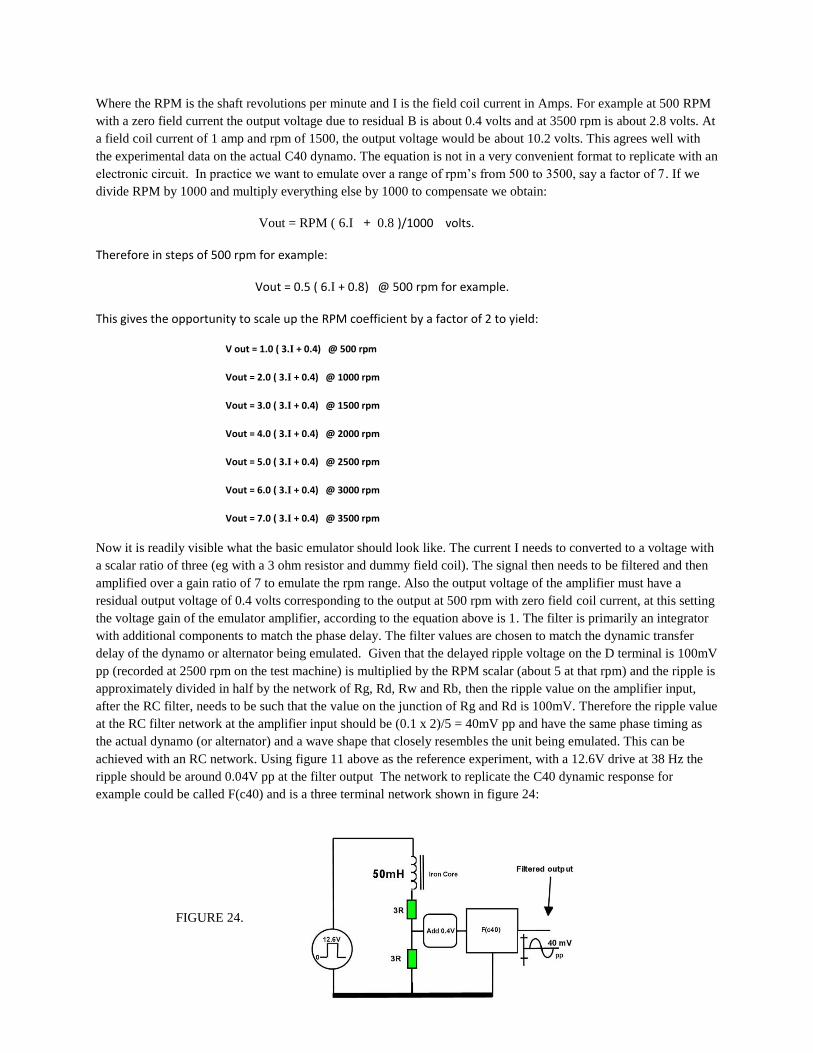
delay of the dynamo or alternator being emulated. Given that the delayed ripple voltage on the D terminal is 100mV

pp (recorded at 2500 rpm on the test machine) is multiplied by the RPM scalar (about 5 at that rpm) and the ripple is

approximately divided in half by the network of Rg, Rd, Rw and Rb, then the ripple value on the amplifier input,

after the RC filter, needs to be such that the value on the junction of Rg and Rd is 100mV. Therefore the ripple value

at the RC filter network at the amplifier input should be (0.1 x 2)/5 = 40mV pp and have the same phase timing as

the actual dynamo (or alternator) and a wave shape that closely resembles the unit being emulated. This can be

achieved with an RC network. Using figure 11 above as the reference experiment, with a 12.6V drive at 38 Hz the

ripple should be around 0.04V pp at the filter output The network to replicate the C40 dynamic response for

example could be called F(c40) and is a three terminal network shown in figure 24:

FIGURE 24.

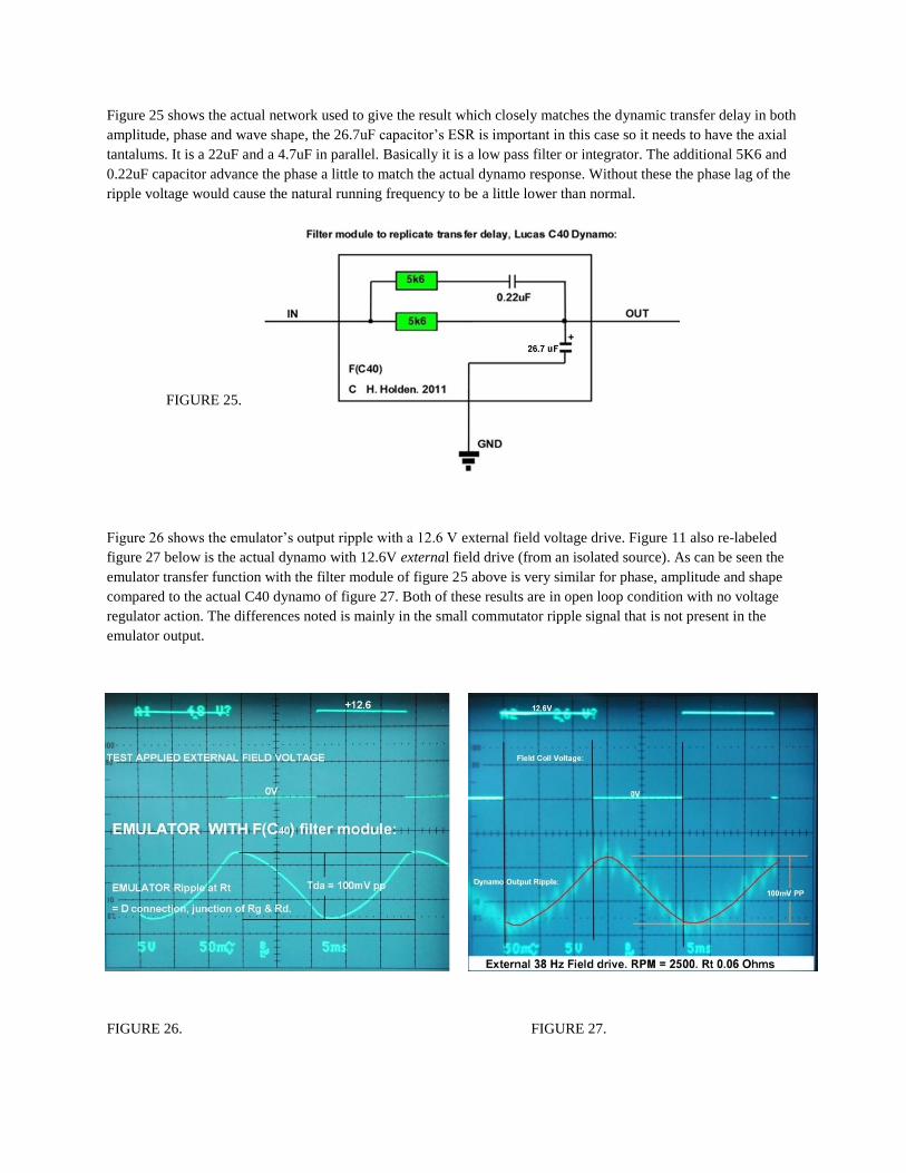
Figure 25 shows the actual network used to give the result which closely matches the dynamic transfer delay in both

amplitude, phase and wave shape, the 26.7uF capacitor’s ESR is important in this case so it needs to have the axial

tantalums. It is a 22uF and a 4.7uF in parallel. Basically it is a low pass filter or integrator. The additional 5K6 and

0.22uF capacitor advance the phase a little to match the actual dynamo response. Without these the phase lag of the

ripple voltage would cause the natural running frequency to be a little lower than normal.

FIGURE 25.

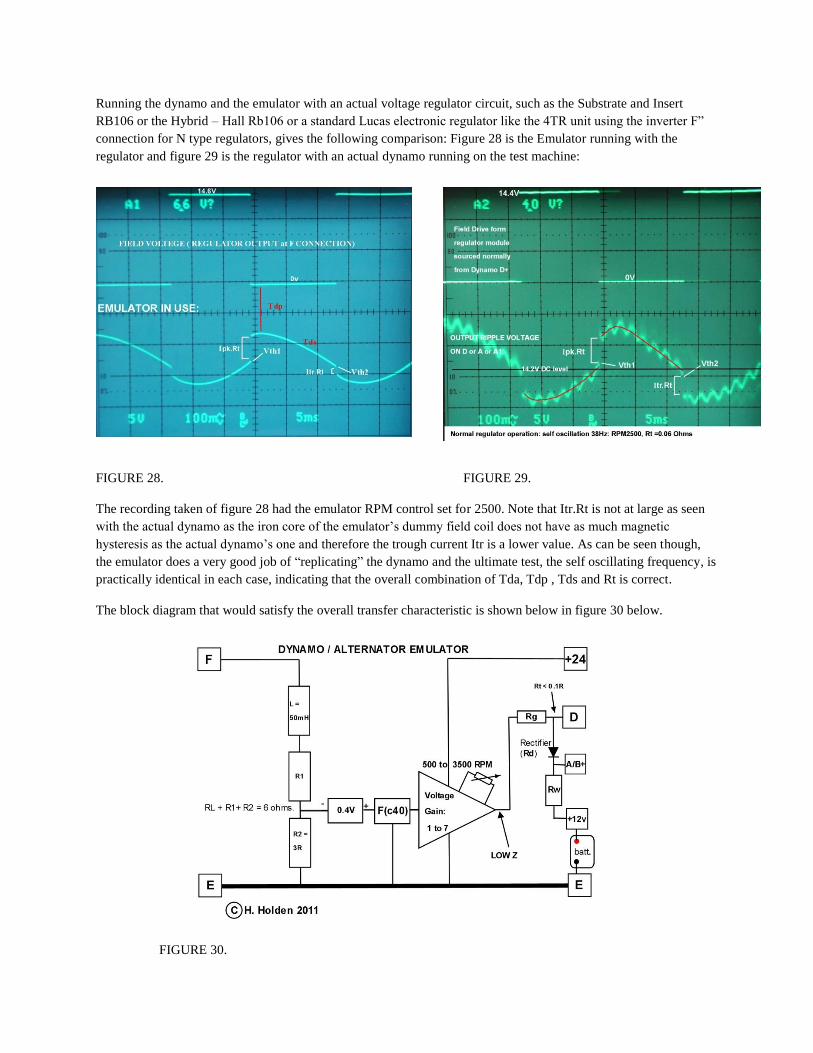
Figure 26 shows the emulator’s output ripple with a 12.6 V external field voltage drive. Figure 11 also re-labeled

figure 27 below is the actual dynamo with 12.6V external field drive (from an isolated source). As can be seen the

emulator transfer function with the filter module of figure 25 above is very similar for phase, amplitude and shape

compared to the actual C40 dynamo of figure 27. Both of these results are in open loop condition with no voltage

regulator action. The differences noted is mainly in the small commutator ripple signal that is not present in the

emulator output.

FIGURE 26. FIGURE 27.

Running the dynamo and the emulator with an actual voltage regulator circuit, such as the Substrate and Insert

RB106 or the Hybrid – Hall Rb106 or a standard Lucas electronic regulator like the 4TR unit using the inverter F”

connection for N type regulators, gives the following comparison: Figure 28 is the Emulator running with the

regulator and figure 29 is the regulator with an actual dynamo running on the test machine:

FIGURE 28. FIGURE 29.

The recording taken of figure 28 had the emulator RPM control set for 2500. Note that Itr.Rt is not at large as seen

with the actual dynamo as the iron core of the emulator’s dummy field coil does not have as much magnetic

hysteresis as the actual dynamo’s one and therefore the trough current Itr is a lower value. As can be seen though,

the emulator does a very good job of “replicating” the dynamo and the ultimate test, the self oscillating frequency, is

practically identical in each case, indicating that the overall combination of Tda, Tdp , Tds and Rt is correct.

The block diagram that would satisfy the overall transfer characteristic is shown below in figure 30 below.

FIGURE 30.

Commercial electronic regulator modules are designed to interface with an inductive load (the field coil or rotor).

The field coil in a C40 dynamo has an inductance of about 50mH and a DC resistance of about 6 ohms. The rotor

coil in a Lucas 35 Amp ACR style alternator has an inductance of about 30mH and a DC resistance of about 4 ohms,

so they are quite similar. Also since the unregulated dynamo or alternator can produce over 20V in the higher rpm

ranges then the emulator needs to be powered by a 24V supply. Two 12V lead acid batteries suffice. A separate 12V

battery is needed to complete the charging circuit and with the wiring and rectifier resistance and the internal

resistance of the artificial generator Rg, creates the overall correct Rt value. The resistors (R1 and R2) in figure 30

ensure that the combination of both the DC resistance and the inductance of the dummy field (or rotor) coil) is

similar to the unit being emulated. Also this gives the option to amplify the field coil current, which is converted to a

voltage across the 3 ohm resistor. This scales the voltage as indicated by the equation by a factor of 3. Then the 0.4

V is added which corresponds to the residual B field magnetism (or the M value) with no field current. The signal is

then filtered to match the dynamic transfer function. Then the output is scaled over a range of 1 to 7 by a variable

gain power amplifier so that the effect of the shaft rpm can be emulated over the range of 500 to 3500.

The power amplifier must be able to provide the total current output without overheating. In the practical emulator

described below this was done with a high current NPN power transistor on a heat-sink which can easily provide 5A

continuous current and overload to 30A for brief periods so as to check current regulator function if a current

regulator is present in the electronic module being tested.

In general alternator regulators are usually only voltage regulators. Some lower power dynamo regulators

incorporate a current limiter to protect the dynamo as used in the Lucas RB106 compensated systems or the 3

bobbin Lucas regulators or in the electronic regulators I have designed such as the ERB106(substrate RB106) or the

Hybrid-Hall RB106.

The actual circuit of the emulator is shown below in figure 31:

FIGURE 31.

The output resistance at the emitter of the BUT92 is very low in the order of 0.01 ohms or less. The combination of

the Rg of 0.165R and Rd and Rw and the battery’s internal resistance Rb, creates a similar Rt to that with the

regulator in use with an actual dynamo and battery and wiring system. Rg was lowered from 0.5R to 0.165R, so as

to lower Rt from 0.08R to 0.06R, in the emulator, to allow for the fact that Ipk and Itr are a little larger (by a factor

of 1.3) for the type of iron cored inductor used (Jaycar laminated iron core) compared to the actual field coil’s

magnetic core of the actual dynamo. This ensures that the value Ipk.Rt and Itr.Rt are practically identical in the

dynamo and emulator charging system.

If this emulator was run in a Spice style program, it is important that the 50mH dummy field coil is iron cored,

otherwise the peak and trough field coil currents will be much higher than usual, increasing Ipk and Itr and this will

lower the running frequency.

My first experimental emulator (figures 32 & 33) was physically constructed on a 10mm thick piece of phenolic

material acquired in Akihabara Japan. Rivets were placed via a 1/8” thick fibreglass panel (USA made) and this

experimental version hard wired and a brass strap used as an earth bus under the board.

FIGURE 32. FIGURE 33.

The 50mH inductor was created from 4 Jaycar 9mH inductors, with two of the coils discarded and the iron

laminations bolted into a “square” ring. Bolting together improves the magnetic circuit the two coils 9mH coils gave

about 50mH in series. The 0.022uF capacitor on the B-C of the 2N4036 is to eliminate any instability at RF

frequencies. Brass knurled nuts were used for low resistance connections to the batteries and various regulators.

A volt meter was attached to the A/B+ terminal. It is also an Amp meter with a Hall current sensor. The currents in

any lead can be measured by passing the lead via the Hall utility. In this emulator the battery charge current is

monitored as it is in a vehicle with an amp meter.

An additional transistor (MJ2955) was added as a power inverter stage as an option for testing N type regulators.

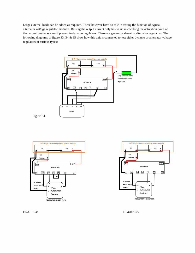
Large external loads can be added as required. These however have no role in testing the function of typical

alternator voltage regulator modules. Raising the output current only has value in checking the activation point of

the current limiter system if present in dynamo regulators. These are generally absent in alternator regulators. The

following diagrams of figure 33, 34 & 35 show how this unit is connected to test either dynamo or alternator voltage

regulators of various types:

Figure 33.

FIGURE 34. FIGURE 35.

The prototype Emulator also includes a 24V 10W bulb connected across the A/B+ terminal and earth. The small

additional current is helpful when testing electro-mechanical regulator, like the RB106, to ensure the cut-out contact

remains solidly closed during testing. Also remember when testing and setting electromechanical regulators that

they are sensitive to their orientation in the gravity field due to forces on the moving arm and this can alter the

voltage setting by as much as 0.5 volts. So they must be adjusted on the same position in that they are mounted in

the vehicle.

Also when testing a N type regulator, as seen in figure 34, as this is interfaced to the emulator by the transistor

inverter utility, it is worth placing a low value resistor, 15 ohms 5w, briefly across the F” and D terminals, to ensure

that the transistor output stage in the N type regulator can saturate satisfactorily with a moderate current load.

One interesting experimental finding with this emulator is that disconnecting the battery in use, which raises Rt from

about 0.062 ohms to around 0.165 ohms results, as expected, the ripple voltage amplitude increasing by about 2.5.

However there is little change in the running frequency because the amplitude increase of Td offsets the increase of

Ipk.Rt and Itr.Rt. This means that it is possible to build an emulator with no actual battery being charged if Rg was

made a low value such as 0.062 Ohms. In other words Rg becomes Rt. However the overall behaviour might be less

predictable.

Summary:

Any type of 12 V electro-mechanical dynamo or alternator voltage regulator or any type of common variable

frequency electronic regulator can be tested with this emulator. Both P and N types can be tested due to the inverter

facility. This emulator would also work to test a fixed frequency regulator too. For the usual variable frequency

regulators, the filter module should be designed so that Tda, Tds and Tdp are close to the unit being emulated. With

an Rt of around 0.06 Ohms the actual emulator output ripple should match that of the unit being emulated.

For those regulators, specifically ones for dynamo’s which have current limiters, an external large load can be

briefly added to check the threshold of current limiter activation. For compensated regulators like the RB106 where

the current loading continuously affects the output voltage the output voltage can be calibrated at a known output

current using the equation published in my article on experimental RB106’s or simply by using the advice for setting

the voltage as given in the manual under no external load (only field current loading) conditions. The emulator can

also be used to set the cut-out adjustment on an electromechanical regulator.

Dr. H. Holden. Oct. 2011.

********************************************************************************************