The early 20th century warming in the Arctic –A possible mechanism

Lennart Bengtsson

Max Planck Institute for Meteorology, Hamburg, Germany

ESSC, University of Reading, UK

Thanks to Vladimir Semenov and Ola M. Johannessen

Johannessen et al. 2003

Temperature anomalies

Possible changes in the distribution of important fish species in the future

Source: Reidar Toresen, IMR

Other speciesNorth Sea herringMackerelCodCapelinNorwegian spring spanning herring

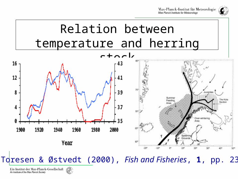
Relation between temperature and herring stock

Source: Toresen & Østvedt (2000), Fish and Fisheries, 1, pp. 231-256

What could be a possible mechanism for the warming event?

Possible explanations for the early century warming

Solar forcing

• Solar irradiation data available for about 20 years only: long-term reconstructions are based on indirect data

• Simulated temperature response to direct solar forcing does not match to the observed pattern of variability and its magnitude (e.g. Cubasch et al., 1997)

• Cosmic radiation – cloud cover hypothesis has been refuted by recent analyses using longer and more comprehensive data sets (e.g. Sun and Bradley, 2002, JGR)

Possible explanations for the early century warming

Volcanic forcing

A series of major eruptions in the early part of the century: Santa Maria (1902), Ksudash (1907), Katmai (1912) then with no substantial eruptions until Mount Agung (1963).

• A cooling effect of a major eruption lasts for 1-3 years

• Neither geographical distribution nor the time evolution of the Arctic SAT correspond to the main volcanic events

• Pinatubo (1991) eruption was twice as powerful as Katmai

• Low latitude eruptions may produce even warming over land in high latitudes in wintertime

Possible explanations for the early century warming

Anthropogenic forcing (greenhouse gases, aerosols)

• The forcing during early decades of the 20th century was only about 20% of the present-day values

• Increasing greenhouse forcing cannot explain 1940-1960 cooling

• Neither geographical distribution nor the magnitude of the aerosol forcing correspond to the 1940-1960 cooling trend pattern

• Global radiative forcing was positive (and even increasing) in the 1940-1960, when the global temperature decreased (Forcing data from Roeckner et al., 1999)

Possible explanations for the early century warming

Natural variability

• Decadal variability of the atmospheric (oceanic) circulation due to aggregation of stochastic events

• Coupled ocean-atmosphere modes (e.g. Delworth and Mann, 2000; Ikeda, 2001; Mysak, 2001)

• Fresh water balance – Arctic sea ice (Zakharov, 1997)

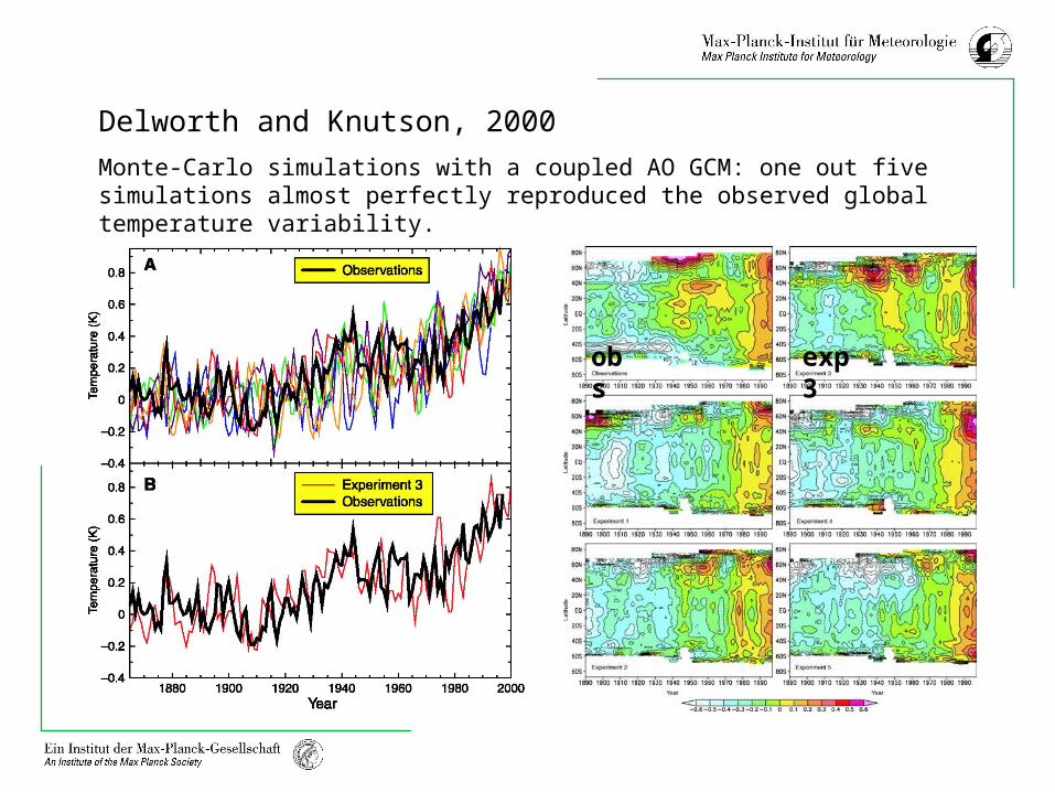
Delworth and Knutson, 2000

Monte-Carlo simulations with a coupled AO GCM: one out five simulations almost perfectly reproduced the observed global temperature variability.

obs exp 3

Johannessen et al. 2003

Temp. Anomalies at

the surface

A

C

B

Statistical analysis

Semenov and Bengtsson, 2003 , JGR

Four leading EOFs of the wintertime (NDJFMA) SAT variability (40N-80N) for 1892-1998

Correlation with atmosph. circulation indices

PC1

NAO (0.60), AO (0.77)

PC2PNA (-0.48), SLP PC2 (-0.57)

PC3

Arctic SAT (0.79)

PC4

SCA (0.33)

1935-1944 wintertime (NDJFMA) Arctic SAT 1935-1944 anomaly, in °C

EOF3 of the wintertime (NDJFMA) Arctic SAT

Arctic SAT (60°N-80°N, NDJFMA) anomalies with subtracted variability (red) related to the EOF1, EOF3 and EOF1+3, and without subtraction (black). 5 years running means

EOF1 and EOF3 explain 94% of the SAT variability north of 60°N

Semenov and Bengtsson (2003)MPI Report 343http://www.mpimet.mpg.de/

Ice area & temperature5-yrs running mean

Johannessen et al. 2003

A link between Arctic SAT and sea ice area

dT/dIce = 1.44 oC/M km2 (annual, Zakharov)

dT/dIce = 0.98 oC/M km2 (annual) or 1.33 oC/M km2 (winter) (Chapman&Walsh)

Sea-ice extent anomalies derived from observations representing ~3/4 of the Arctic Ocean (Zakharov, 1997), compared with annual Arctic (60N-90N) SAT.

Empirical data analysis: summary

• The early century warming in the Arctic was most pronounced during winter and had a very distinguished spatial pattern with maximum warming over the Barents and Kara Seas.

• Variability associated with the early century warming pattern shows no link to the large-scale atmospheric circulation variability.

• There is a strong link between SAT and sea ice area variability in the Arctic. The Barents Sea is characterized by strong variability of the wintertime ice cover.

• The sea ice cover variability (basically in the Barents Sea) is suggested to be a reason for the early century warming.

Atmospheric model simulations: experimental setup

• atmospheric general circulation model ECHAM4

• 19 vertical levels

• spatial resolution of approximately 2.8 deg in lat/lon

• an ensemble of four simulations using the GISST2.2 SST/SIC analysis for 1903-1994 (Rayner et al., 1996) as boundary conditions was carried out

• observed changes in the greenhouse gases concentrations were included

• the experiments started from slightly different initial atmospheric states but had all identical boundary conditions

Atmospheric model simulations: sea ice data

Annual mean Arctic sea ice areaGISST2.2: wintertime SIC difference (in%)

between the 1954-1983 and 1910-1939 averages

Atmospheric model simulations: temperature changes

Wintertime Arctic SAT anomalies simulated by 4 ensemble experiments with ECHAM4 model

Wintertime SAT difference between 1910-39 and 1954-83 means

cor (Ice,SAT) = -0.59 (wintertime 1951-1994)

dT/dIce = 0.67 oC/M km2 (wintertime)

ΔT/ΔIce = 1.13 oC/M km2

Atmospheric model simulations: circulation changes

SIC Heat flux, W/m2

SLP, mb 10m wind

Atmospheric model simulations: circulation changes

Atmospheric model simulations: summary

• Simulated Arctic temperature showed a strong dependence on the prescribed sea ice changes with 1.13 ºC SAT increase corresponding to 1Mkm2 sea ice area decrease (wintertime). This is similar to the observed value (1.33).

• A pattern of the SAT change is very similar to the observed pattern with major changes in the Barents Sea.

• A reduced sea ice cover in the Barents Sea causes a cyclonic atmospheric circulation in the Barents Sea region associated with enhanced westerly winds between Norway and Spitsbergen.

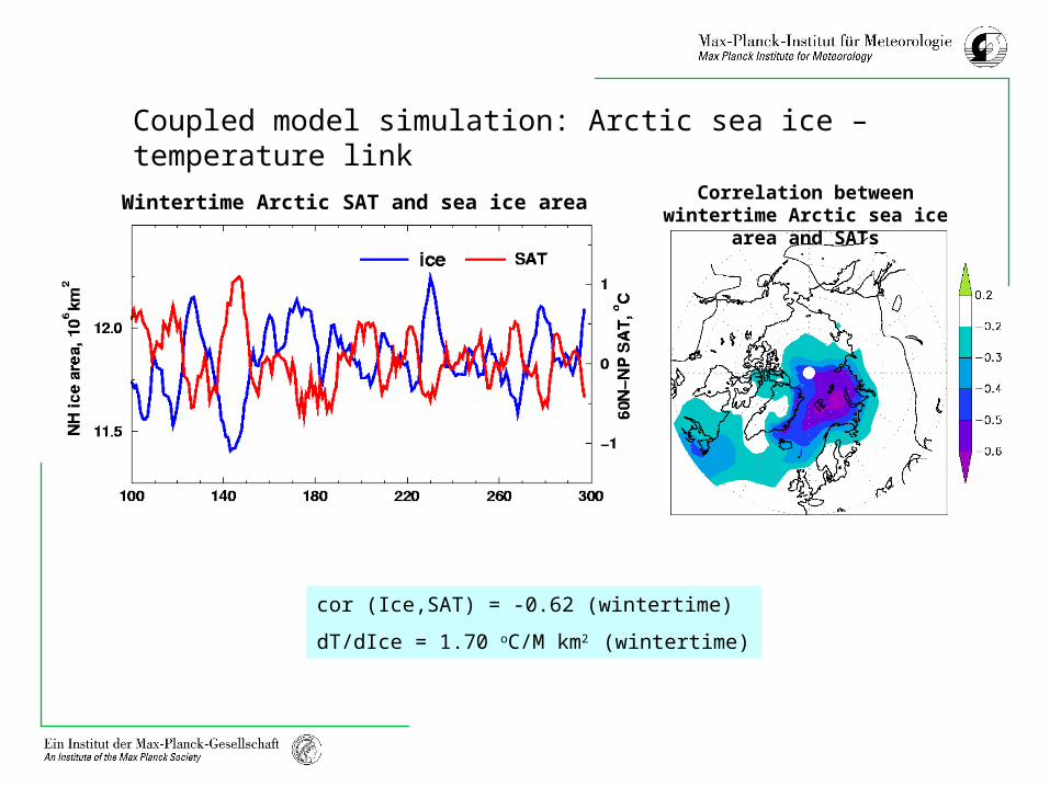
Coupled model simulation: Arctic sea ice – temperature link

Wintertime Arctic SAT and sea ice area Correlation between wintertime Arctic sea ice area and SATs

cor (Ice,SAT) = -0.62 (wintertime)

dT/dIce = 1.70 oC/M km2 (wintertime)

Coupled model simulation: Barents Sea inflow

Annual mean Arctic sea ice area anomalies and oceanic volume flux (upper 125 m) through Spitzbergen-Norway meridional (about 20E) cross-section

r = -0.77

Coupled model simulation: Barents Sea inflow

Annual mean oceanic volume flux and DJF SLP difference Spitzbergen-northern Norway

r = 0.42

Coupled model simulation: summary

• Simulated Arctic temperature showed a strong link to the sea ice changes with 1.70 ºC SAT increase corresponding to 1Mkm2 sea ice area decrease (wintertime). This is similar to the observed value (1.33).

• A pattern of the SAT change is very similar to the observed pattern with major changes in the Barents Sea, where the highest variability of the ice cover occurs.

• Variability of the sea ice cover in the Barents Sea are caused by changes of the oceanic inflow through the western opening of the sea.

• The inflow variability is linked to the strength of westerlies north of Norway.

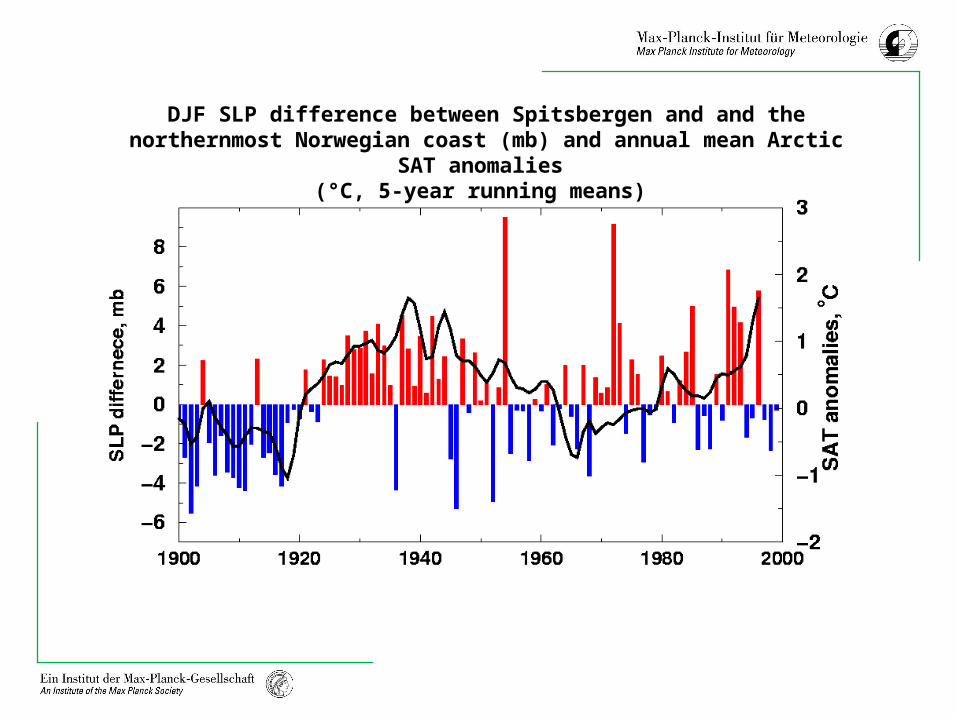
DJF SLP difference between Spitsbergen and and the northernmost Norwegian coast (mb) and annual mean Arctic SAT anomalies

(°C, 5-year running means)

Spitsbergen-Norway DJF SLP difference

NAO index

Barents inflowBarents Sea

Cyclonic circulation

Westerly winds

Feedback mechanism scheme

Correlation between Arctic wintertime SAT anomalies and DJF SLP (1920-1970)

Conclusions

• A reduced sea ice cover (mainly in the Barents Sea) is the main cause of the warming

• The ice retreat was caused by enhanced wind driven oceanic inflow into the Barents Sea

• The increased inflow can be explained by intensified westerly winds between Spitsbergen and the Norwegian coast in 1920s-1940s

• A positive feedback is proposed sustaining the enhanced westerly winds by a cyclonic atmospheric circulation in the Barents Sea region created by a strong surface heat flux over the ice-free areas

Recent numerical experiments: sea-ice and temperature

Experiments with the atmospheric GCM ECHAM5 (T31L19)

20th century climate simulations:

1) ensemble runs with HadISST1 SST/sea ice concentration data (1950-1998)

Sensitivity experiments:

1) experiments with constant sea ice / SST

2) climatological experiments with regionally reducing sea ice cover (e.g. in the Barents Sea)

3) “ice free Arctic” experiment

ECHAM5/HadISST1 ensemble runs: Arctic wintertime SAT anomalies, °C (black – observed, Jones)

ECHAM5/HadISST1 ensemble runs: SLP difference Azores-Iceland, mb

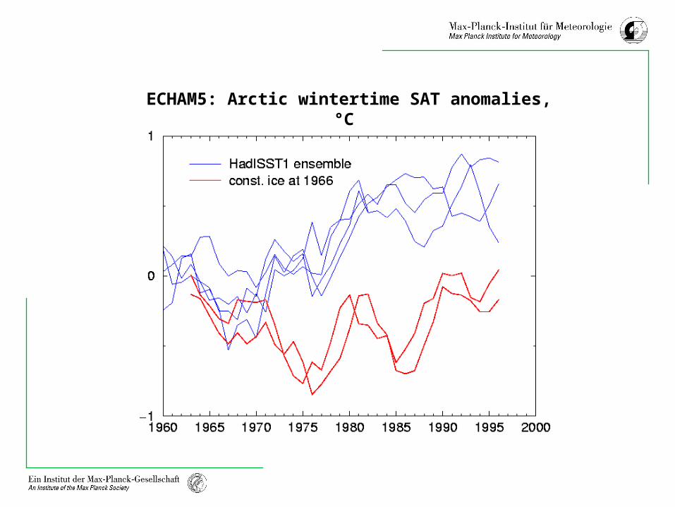
ECHAM5: Arctic wintertime SAT anomalies, °C

ECHAM5 “ice free Arctic” experiment:Wintertime SAT difference ice free – AMIP ice

END