The econometrics of inequality and povertyLecture 10: Explaining poverty and inequality using

econometric models

Michel Lubrano

October 2016

Contents

1 Introduction 3

2 Decomposing poverty and inequality 32.1 FGT indices . . . . . . . . . . . . . . . . . . . . . . . . . . . . . . . . . . . . . 32.2 Generalised entropy indices . . . . . . . . . . . . . . . . . . . . . . .. . . . . . 42.3 Oaxaca decomposition . . . . . . . . . . . . . . . . . . . . . . . . . . . . .. . 62.4 Oaxaca inR . . . . . . . . . . . . . . . . . . . . . . . . . . . . . . . . . . . . . 82.5 Explaining the income-to-needs ratio . . . . . . . . . . . . . . .. . . . . . . . . 112.6 A model for poverty dynamics . . . . . . . . . . . . . . . . . . . . . . . .. . . 15

3 Models for income dynamics 153.1 Income dynamics . . . . . . . . . . . . . . . . . . . . . . . . . . . . . . . . . .163.2 Transition matrices and Markov models . . . . . . . . . . . . . . .. . . . . . . 173.3 Building transition matrices . . . . . . . . . . . . . . . . . . . . . .. . . . . . . 183.4 What is social mobility: Prais (1955) . . . . . . . . . . . . . . . .. . . . . . . . 193.5 Estimating transition matrices . . . . . . . . . . . . . . . . . . . .. . . . . . . 223.6 Distribution of indices . . . . . . . . . . . . . . . . . . . . . . . . . . .. . . . 233.7 Modelling individual heterogeneity using a dynamic multinomial logit model . . 243.8 Transition matrices and individual probabilities . . . .. . . . . . . . . . . . . . 26

4 Introducing and illustrating quantile regressions 274.1 Classical quantile regression . . . . . . . . . . . . . . . . . . . . .. . . . . . . 274.2 Bayesian inference . . . . . . . . . . . . . . . . . . . . . . . . . . . . . . .. . 284.3 Quantile regression using R . . . . . . . . . . . . . . . . . . . . . . . .. . . . . 284.4 Analysing poverty in Vietnam . . . . . . . . . . . . . . . . . . . . . . .. . . . 29

1

5 Marginal quantile regressions 305.1 Influence function . . . . . . . . . . . . . . . . . . . . . . . . . . . . . . . .. . 305.2 Marginal quantile regression . . . . . . . . . . . . . . . . . . . . . .. . . . . . 31

6 Appendix 34

A Quantile regressions in full 34A.1 Introduction . . . . . . . . . . . . . . . . . . . . . . . . . . . . . . . . . . . .. 34A.2 Applications . . . . . . . . . . . . . . . . . . . . . . . . . . . . . . . . . . . .. 36

B Statistical inference 37B.1 Inference Bayesienne . . . . . . . . . . . . . . . . . . . . . . . . . . .. . . . . 39B.2 Non-parametric inference . . . . . . . . . . . . . . . . . . . . . . . . .. . . . . 40

B.2.1 L’estimation nonparametrique des quantiles . . . . . .. . . . . . . . . . 40B.2.2 Regression quantile non-parametrique . . . . . . . . . .. . . . . . . . . 41

2

1 Introduction

Up to now, we focussed on the description of the income distribution. We saw how to comparetwo distributions, either between two different countriesor for the same country between twodifferent points of time. But we stayed on a descriptive standpoint, we did not try to explainthe formation of the income distribution or to explain poverty. In doing this, we followed thedichotomy that exists in the literature between measuring inequality and poverty and the theoryof income formation. Household income can be divided in several parts: wages or earning(the most important part of income), rents and financial income and finally taxes and transfers.Labour economists examined the question of wage inequalityand wage dispersion in the eighties,promoting for instance the dichotomy between skilled and unskilled labour. However, they havenever tried to relate this question to household income inequality. We shall not try to fill up thegap in this chapter, asking the reader to refer to Atkinson (2003) for instance. We shall howevertry to present some econometric tools that are useful for decomposing a poverty index or foranalysis the evolution of an income distribution.

2 Decomposing poverty and inequality

The idea is to split the inequality or the poverty measured byan index into different and mutualityexclusive groups. Which group in the population is more subject to poverty? This principle canbe extended to the decomposition of inequality, most of the time wage inequality in the literature,between two groups. For instance is wage differential between male and females or black andwhite due to intrinsic differences or to a mere discrimination? For that, we need a wage equation,a model based on a regression and then to decompose the regression between different effects.This is the Oaxaca decomposition.

2.1 FGT indices

The index of Foster et al. (1984) is decomposable because of its linear structure. Let us considerthe decomposition of a population between rural and urban. If X represents all income of thepopulation, the partition ofX is defined asX = XU +XR. Let us callp the proportion ofXU

in X. Then the total index can be decomposed into

Pα = p1

n

nU∑

i=1

(z − xU

i

z

)α

1I(xi ≤ z) + (1− p)1

n

nR∑

i=1

(z − xR

i

z

)α

1I(xi ≤ z) (1)

= p PUα + (1− p)PR

α . (2)

wherePUα is the index computed for the urban population andPR

α the index computed for the ru-ral population. So decomposition for a poverty index means that poverty for the total populationcan be expressed as a weighted sum of the same poverty index applied to each group. Inequalityindices can also be decomposed. But here, as we have already seen in Chapter 7, decomposabil-ity means something else. Inequality within the total population is expressed as a weighted sum

3

of inequality within each group plus a remainder which is interpreted as inequality between thegroups.

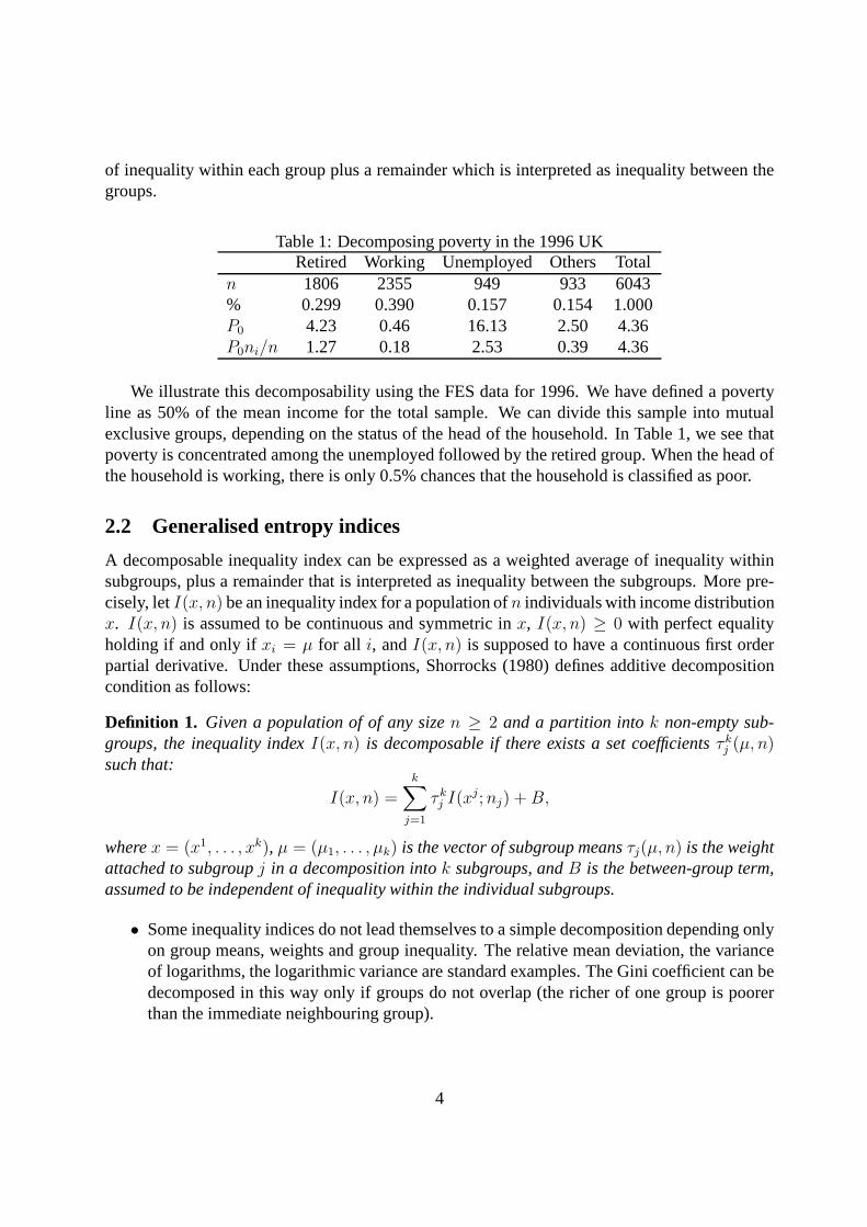
Table 1: Decomposing poverty in the 1996 UKRetired Working Unemployed Others Total

n 1806 2355 949 933 6043% 0.299 0.390 0.157 0.154 1.000P0 4.23 0.46 16.13 2.50 4.36P0ni/n 1.27 0.18 2.53 0.39 4.36

We illustrate this decomposability using the FES data for 1996. We have defined a povertyline as 50% of the mean income for the total sample. We can divide this sample into mutualexclusive groups, depending on the status of the head of the household. In Table 1, we see thatpoverty is concentrated among the unemployed followed by the retired group. When the head ofthe household is working, there is only 0.5% chances that thehousehold is classified as poor.

2.2 Generalised entropy indices

A decomposable inequality index can be expressed as a weighted average of inequality withinsubgroups, plus a remainder that is interpreted as inequality between the subgroups. More pre-cisely, letI(x, n) be an inequality index for a population ofn individuals with income distributionx. I(x, n) is assumed to be continuous and symmetric inx, I(x, n) ≥ 0 with perfect equalityholding if and only ifxi = µ for all i, andI(x, n) is supposed to have a continuous first orderpartial derivative. Under these assumptions, Shorrocks (1980) defines additive decompositioncondition as follows:

Definition 1. Given a population of of any sizen ≥ 2 and a partition intok non-empty sub-groups, the inequality indexI(x, n) is decomposable if there exists a set coefficientsτkj (µ, n)such that:

I(x, n) =

k∑

j=1

τkj I(xj;nj) +B,

wherex = (x1, . . . , xk), µ = (µ1, . . . , µk) is the vector of subgroup meansτj(µ, n) is the weightattached to subgroupj in a decomposition intok subgroups, andB is the between-group term,assumed to be independent of inequality within the individual subgroups.

• Some inequality indices do not lead themselves to a simple decomposition depending onlyon group means, weights and group inequality. The relative mean deviation, the varianceof logarithms, the logarithmic variance are standard examples. The Gini coefficient can bedecomposed in this way only if groups do not overlap (the richer of one group is poorerthan the immediate neighbouring group).

4

• The class of decomposable indices contains many examples. We can quote the inequal-ity index of Kolm which has an additive invariance property (when usual indices have amultiplicative invariance property). The widest class of decomposable inequality indicesis represented by the Generalised Entropy indices which contains as particular cases theTheil index, the mean logarithm deviation index and the Atkinson index.

We consider a finite discrete sample ofn observations divided exactly ink groups. Eachgroup has proportionpi, sizeni and empirical meanµi. Inside a group, the generalised entropyindex writes

IGEi=

1

c2 − c

[ni∑

j=1

pi

(yjµi

)c

− 1

]

Inequality between groups is measured as

IBetween =1

c2 − c

[k∑

i=1

pi

(µi

µ

)c

− 1

]

whereµ is the sample mean. Let us now define the income share of each group as

gi = piµi

µ

Then inequality is decomposed according to

ITotal =

k∑

i=1

gcip1−ci IGEi

+ IBetween

The Atkinson index is a non-linear function of the GE index. Consequently the decompositionof this index is ordinaly but not cardinally equivalent to the decomposition of the GE. For detailsof calculation, see Cowell (1995).

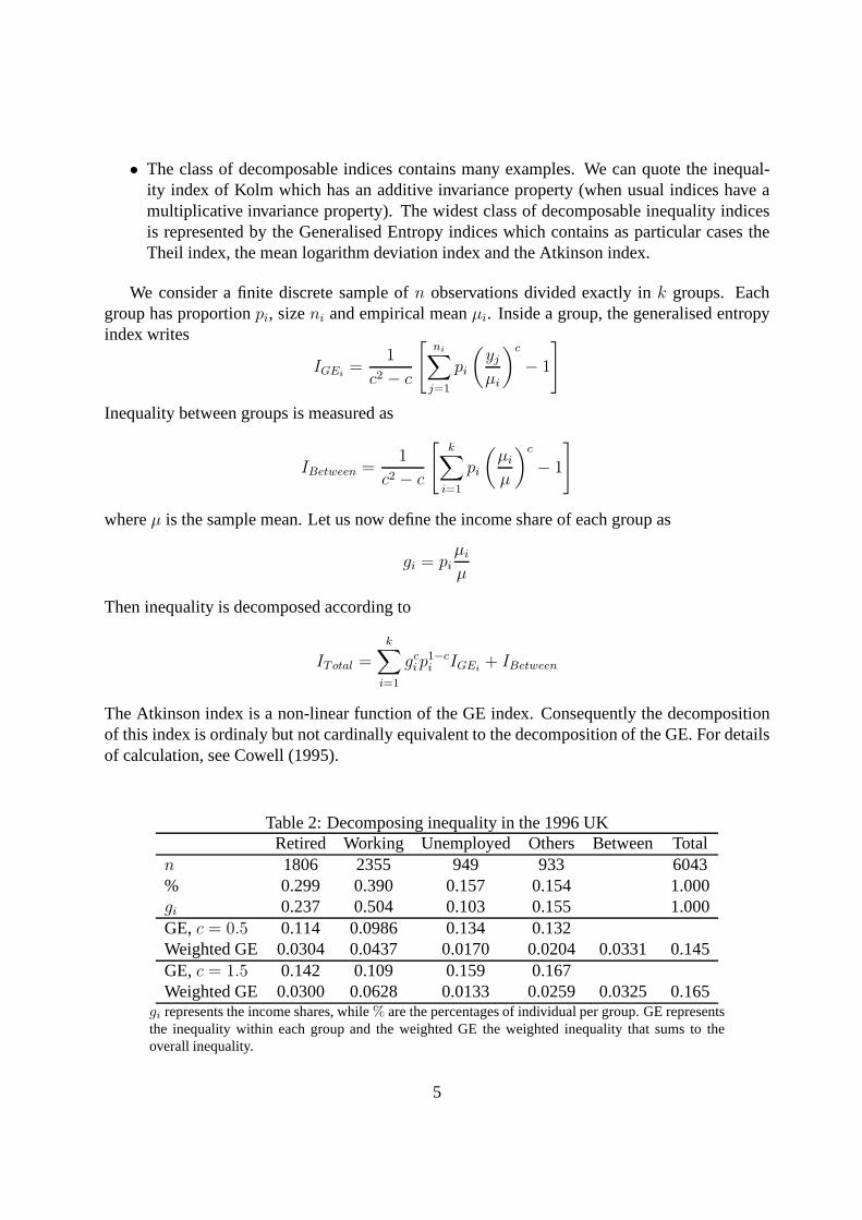
Table 2: Decomposing inequality in the 1996 UKRetired Working Unemployed Others Between Total

n 1806 2355 949 933 6043% 0.299 0.390 0.157 0.154 1.000gi 0.237 0.504 0.103 0.155 1.000GE,c = 0.5 0.114 0.0986 0.134 0.132Weighted GE 0.0304 0.0437 0.0170 0.0204 0.0331 0.145GE,c = 1.5 0.142 0.109 0.159 0.167Weighted GE 0.0300 0.0628 0.0133 0.0259 0.0325 0.165

gi represents the income shares, while% are the percentages of individual per group. GE representsthe inequality within each group and the weighted GE the weighted inequality that sums to theoverall inequality.

5

We illustrate this decomposability using again the FES datafor 1996. We have again dividedthe sample into mutual exclusive groups, depending on the status of the head of the household.In Table 2, we see that weighted inequality is concentrated among the working people accordingto both indices, followed by the retired. On the contrary, there is very little inequality amongthe unemployed. The between inequality is of the same importance as within inequality for theretired. This is just the reverse picture as for poverty.

2.3 Oaxaca decomposition

In the previous section, we have decomposed a poverty rate according to mutually exclusivegroups of the population. But, we provided no explanation onthe reason of this decomposition,what made a person belong to one of these groups. Oaxaca (1973) was the first to try to givean explanation on the sources, the causes of inequality, using a regression model. But note alsothe paper Blinder (1973) published the same year, so that thedecomposition is often called theBlinder-Oaxaca decomposition.

Oaxaca (1973) took interest in wage inequality between males and females. Suppose that wehave divided our sample in two groups, one group of males, onegroup of females. We want toexplain the difference in average wage that there exist between males and females, with the maininterrogation: is this wage differential simply due to differences in characteristics, for instancemales are more educated or have more experience, or is this difference due to discrimination,e.g. the yield of experience is lower for females. In order toanswer these questions, we estimatefor each group a wage equation which relates the log of the wage to a number of characteristics,among which we find experience and years of schooling. Other variables can include regionallocation and city size for instance:

log(Wi) = Xiβi + ui, i = m, f.

Once these two equations are estimated, we have aβm for males and aβf for females. We aregoing to try to explain wages differences between males and females as follows. We can say thata part of this difference can be explained by different characteristics. For instance if males havemore experience or if females are more educated. These objective differences are measured byXh−Xf . But another part of the wage differences can be explained simply by the different yieldof these characteristics: for an identical experience, a female is paid less than a male. Thesedifferences in yields are at the root of the discrimination existing between males and females onthe labour market.

In a regression model, the mean of the endogenous variable isgiven by

log(W i) = X iβi,

because of the zero mean assumption on the residuals. Using this property, Oaxaca proposed thefollowing decomposition:

log(Wm)− log(W f) = (Xm −Xf )βm +Xf (βm − βf).

6

In this decomposition, the difference in percentage between the average male and female wages isexplained first by the difference in average characteristics. As a second term comes the differencein yield of female average characteristics expressed byβm − βf .

This decomposition is very popular in the literature. The original paper is cited more than3171 times (using GoogleScholar). It gave birth to many subsequent developments. For instance,Juhn et al. (1993) generalised the previous result to the framework of quantile regression. Rad-chenko and Yun (2003) provide a Bayesian implementation that make easier significance tests.

There are more than one way of decomposing wage inequality. We have chosen Oaxaca(1973) decomposition. The decomposition promoted by Blinder (1973) is also possible. Thisdual decomposition can be imbedded in a single formulation where the difference in means isexpressed as

log(Wm)− log(W f ) = (Xm −Xf)β∗ + [Xm(βm − β∗) + Xf(β∗ − βf)]. (3)

The first part is the explained part, while the term in squaredbrackets is the unexplained part.We recover the previous decomposition forβ∗ = βm while the Blinder decomposition is foundfor β∗ = βf . Other decomposition found in the literature chooseβ∗ as the average between thetwo regression coefficients.

Of course, a natural question is to know if those differencesare statistically significant. Jann(2008) proposes to compute standard errors for this decomposition. There are various ways ofcomputing these standard deviations, the question being toknow if the regressors are stochasticor not. If the regressors are fixed, then we have the simple result

Var(Xβ) = X ′Var(β)X.

If the regressors are stochastic, but however uncorrelated, Jann shows that this variance becomes

Var(Xβ) = X ′Var(β)X + β ′Var(X)β + tr(Var(X)Var(β)).

From these expressions, he derives the variance of the Oaxaca decomposition. This is simple,but tedious algebra. So it is better to have a ready made program. A command exists in Stata.It was only very recently implemented inR with the packageoaxaca (2014) by Marek Hlavacfrom Harvard (Hlavac 2014). It reproduces the estimation methods available in the Stat package,provide bootstrap standard deviations and also nice plots.

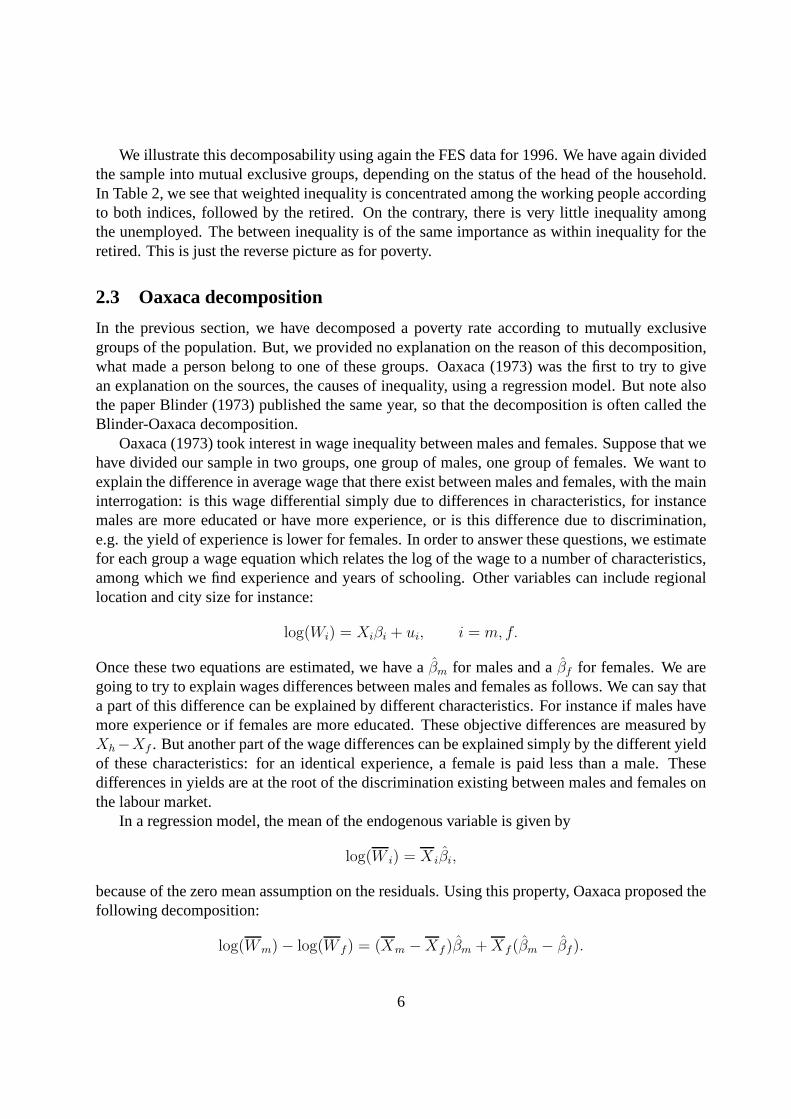
Jann illustrates his method for decomposing the gender wagegap on the Swiss labour marketusing the Swiss Labour Force Survey 2000 (SLFS; Swiss Federal Statistical Office). The sampleincludes Employees aged 20-62, working fulltime, having only one job. The dependent variableis the Log of hourly wages. The explanatory variables are thenumber of years of schooling,the number of years of experience, its square divided by 100,two dummy variables concerningTenure and the gender of the supervisor. There are 3383 malesand 1544 females. From theestimates reported in Table 3, we can compute the original Oaxaca decomposition with resultsdisplayed in Table 4. The bootstrap and the stochastic regressor assumption give very compara-ble standard deviations. Assuming fixed regressors under-evaluate the standard deviations. Wage

7

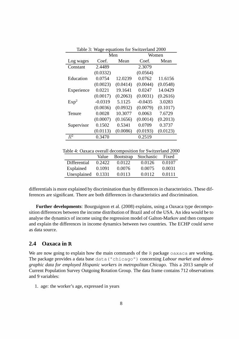
Table 3: Wage equations for Switzerland 2000Men Women

Log wages Coef. Mean Coef. MeanConstant 2.4489 2.3079

(0.0332) (0.0564)Education 0.0754 12.0239 0.0762 11.6156

(0.0023) (0.0414) (0.0044) (0.0548)Experience 0.0221 19.1641 0.0247 14.0429

(0.0017) (0.2063) (0.0031) (0.2616)Exp2 -0.0319 5.1125 -0.0435 3.0283

(0.0036) (0.0932) (0.0079) (0.1017)Tenure 0.0028 10.3077 0.0063 7.6729

(0.0007) (0.1656) (0.0014) (0.2013)Supervisor 0.1502 0.5341 0.0709 0.3737

(0.0113) (0.0086) (0.0193) (0.0123)R2 0.3470 0.2519

Table 4: Oaxaca overall decomposition for Switzerland 2000Value Bootstrap Stochastic Fixed

Differential 0.2422 0.0122 0.0126 0.0107Explained 0.1091 0.0076 0.0075 0.0031Unexplained 0.1331 0.0113 0.0112 0.0111

differentials is more explained by discrimination than by differences in characteristics. These dif-ferences are significant. There are both differences in characteristics and discrimination.

Further developments: Bourguignon et al. (2008) explains, using a Oaxaca type decompo-sition differences between the income distribution of Brazil and of the USA. An idea would be toanalyse the dynamics of income using the regression model ofGalton-Markov and then compareand explain the differences in income dynamics between two countries. The ECHP could serveas data source.

2.4 Oaxaca inR

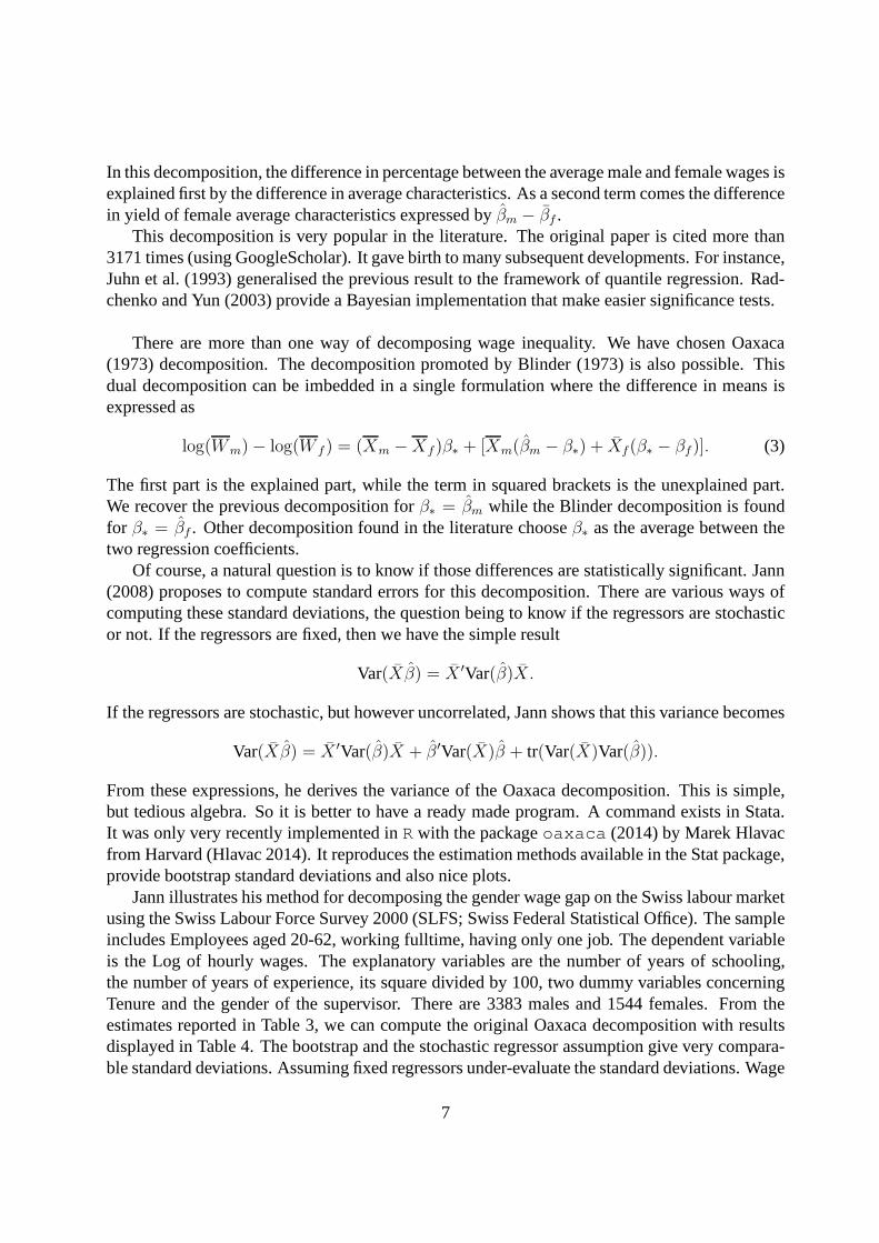
We are now going to explain how the main commands of theR packageoaxaca are working.The package provides a data basedata("chicago") concerningLabour market and demo-graphic data for employed Hispanic workers in metropolitanChicago. This a 2013 sample ofCurrent Population Survey Outgoing Rotation Group. The data frame contains 712 observationsand 9 variables:

1. age: the worker’s age, expressed in years

8

2. female: an indicator for female gender

3. foreign.born: an indicator for foreign-born status

4. LTHS: an indicator for having completed less than a high school (LTHS) education

5. high.school: an indicator for having completed a high school education

6. some.college: an indicator for having completed some college education

7. college: an indicator for having completed a college education

8. advanced.degree: an indicator for having completed an advanced degree

9. ln.real.wage: the natural logarithm of the worker’s realwage (in 2013 U.S. dollars)

The question is to know the impact of being born in a foreign country can explain wage differ-entials. So the main command isoaxaca . To interpret correctly the data, we have first to deletethe rows of the data set that have NA. This is the case only in column 9, which corresponds towages. Then we recreate a new data set

data("chicago")id = !is.na(chicago[,9])chicago = chicago[id,]attach(chicago)n = length(age)

age2 = ageˆ2/100lwage = ln.real.wagewage = exp(lwage)idf = foreign.born==1idn = foreign.born==0sum(idn)sum(idf)mean(wage[idf],na.rm=T)mean(wage[idn],na.rm=T)

Chic = data.frame(wage,age,age2,female,college,advanced.degree,foreign.born)out = oaxaca(wage ˜ age + age2 + female +

college + advanced.degree | foreign.born,data = Chic, R = 30)

The wage equation is described in a formula framework while the group indicator variable isgiven after the vertical bar. Standard errors are estimatedby bootstrap withR = 30 replications.It is not wise to try to print the whole object. It is better to print only some elements.res being

9

here the name of the object, we can first access the useful sample sizes by typingres$n . Thereare missing observations in the wage variable so that at the end there are only 666 observationsleft, with nA = 287 natives andnB = 379 foreign born.

Then, the mean values of the endogenous variable for the two groups is obtained withres$ymean wage is $17.58 for natives and $14.56 for foreign born. The difference is also indicated(3.02).

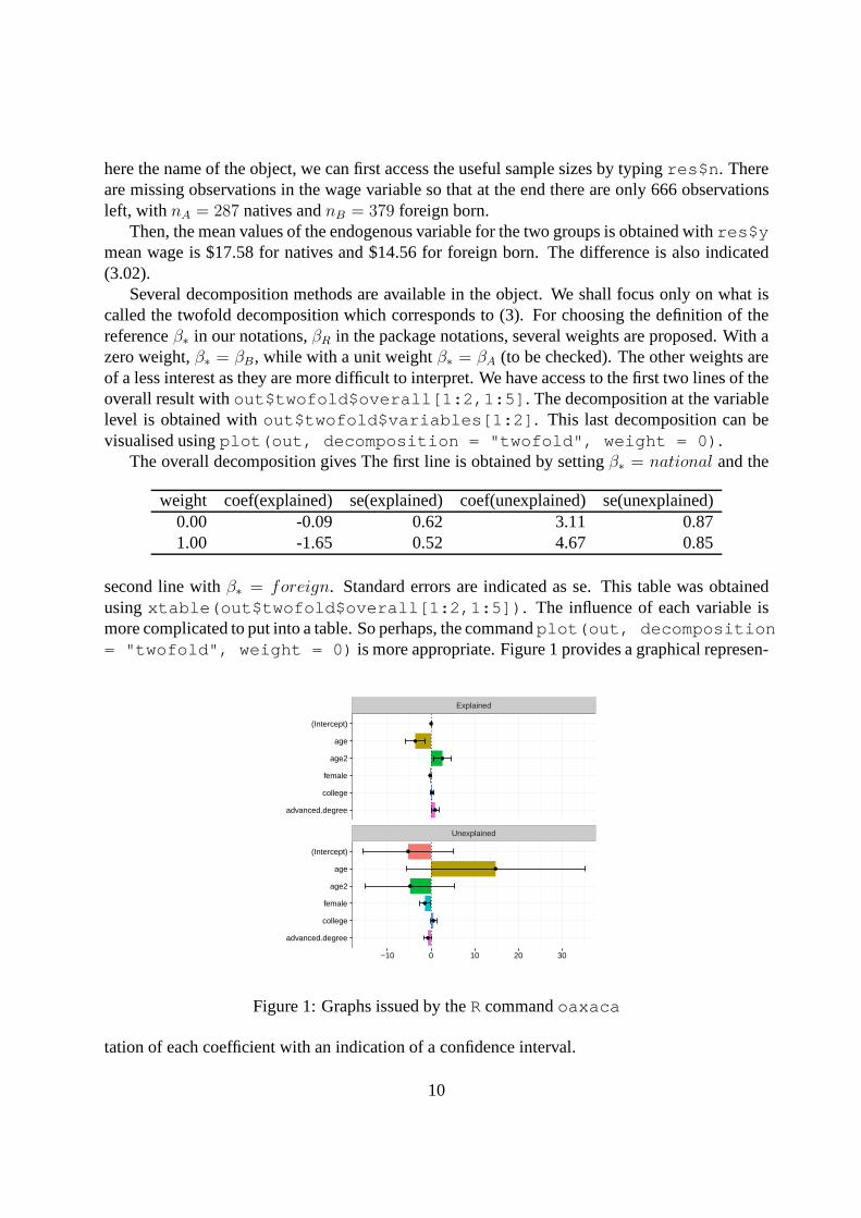
Several decomposition methods are available in the object.We shall focus only on what iscalled the twofold decomposition which corresponds to (3).For choosing the definition of thereferenceβ∗ in our notations,βR in the package notations, several weights are proposed. With azero weight,β∗ = βB, while with a unit weightβ∗ = βA (to be checked). The other weights areof a less interest as they are more difficult to interpret. We have access to the first two lines of theoverall result without$twofold$overall[1:2,1:5] . The decomposition at the variablelevel is obtained without$twofold$variables[1:2] . This last decomposition can bevisualised usingplot(out, decomposition = "twofold", weight = 0) .

The overall decomposition gives The first line is obtained bysettingβ∗ = national and the

weight coef(explained) se(explained) coef(unexplained)se(unexplained)0.00 -0.09 0.62 3.11 0.871.00 -1.65 0.52 4.67 0.85

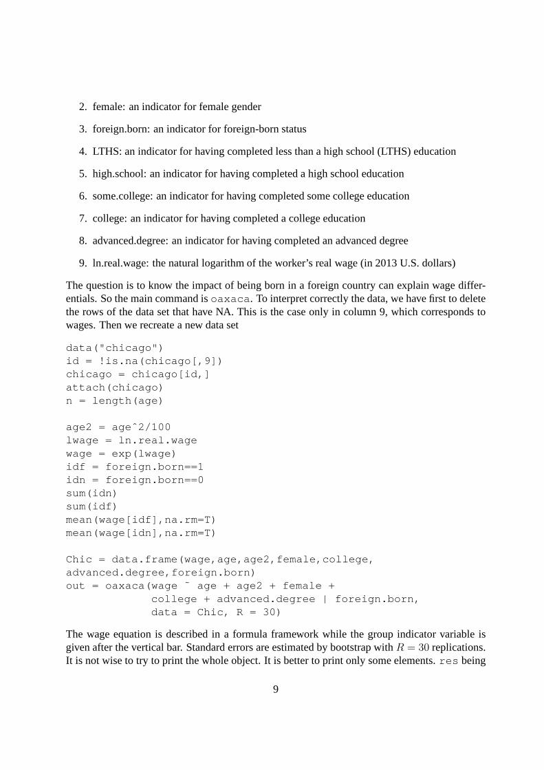
second line withβ∗ = foreign. Standard errors are indicated as se. This table was obtainedusingxtable(out$twofold$overall[1:2,1:5]) . The influence of each variable ismore complicated to put into a table. So perhaps, the commandplot(out, decomposition= "twofold", weight = 0) is more appropriate. Figure 1 provides a graphical represen-

Explained

Unexplained

advanced.degree

college

female

age2

age

(Intercept)

advanced.degree

college

female

age2

age

(Intercept)

−10 0 10 20 30

Figure 1: Graphs issued by theRcommandoaxaca

tation of each coefficient with an indication of a confidence interval.

10

2.5 Explaining the income-to-needs ratio

Let us consider a poverty linez and the incomeyi of an household. The ratioy/z is known tobe theincome-to-needs ratioin the literature. It can be used to explain the probability that thishousehold has of getting in a state of poverty.log(yi/z) is negative if the household is poor,positive otherwise. We can then estimate a regression

log(yi/z) = x′iβ + ui

wherexi is a set of characteristics of the household. If we suppose that ui is normal, we cancompute the probability that an household is poor by mean of

P0 = Pr(xiβ < 0) = Φ(−xiβ/σ)

whereσ2 is the variance of the residuals andΦ(·) the normal cumulative distribution. Whenntends to infinity, the estimated variance tends to zero so that this probability approaches the headcount measure.

We can now extend the approach of Oaxaca to explain the difference that there exist of beingpoor between two groups: white and black households in the USor between Serbs and Albanianhouseholds in Kosovo. Yun (2004) propose a generalisation of Oaxaca decomposition for non-linear models and in particular for probit models. Let us call A andB the two groups we consider.The decomposition proposed by Yun (2004) is as follows:

P 0A − P 0

B = Φ(−XAβA/σA)− Φ(−XBβB/σB)]

= [Φ(−XAβA/σA)− Φ(−XBβA/σA)]

+ [Φ(−XBβA/σA)− Φ(−XBβB/σB)].

which corresponds to the difference between the characteristics and the difference between thecoefficients. This is an overall decomposition, giving global figures. We could be interestingin detailing the influence of each variable in this decomposition. This is not straightforward,because we are in a non-linear model. Yun (2004) has proposeda method to circumvent thisdifficulty by defining a series of weights. Assuming that there arek characteristics or exogenousvariables, we can write

P 0A − P 0

B =∑k

i=1Wi∆X [Φ(−XAβA/σA)− Φ(−XBβA/σA)]

+∑k

i=1Wi∆β[Φ(−XBβA/σA)− Φ(−XBβB/σB)]

Of course the question is how to define those weights. The weightsW i∆X andW i

∆β are given inBhaumik et al. (2006a) following a linearisation argument developed in Yun (2004). They are(to be checked):

W i∆β =

Xi(βAi − βB

i )∑ki=1 Xi(βA

i − βBi )

W i∆X =

βBi (X

Ai − XB

i )∑ki=1 β

Bi (X

Ai − XB

i ).

As an alternative and simpler method, one could consult Bazen and Joutard (2013), which isbased on a Taylor expansion.

11

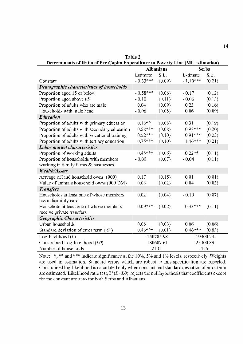
Bhaumik et al. (2006b) use the 2001 Living Standards Measurement Survey (LSMS) data forKosovo to decompose the difference in the average likelihood of poverty incidence between Serband Albanian households. The survey, which was carried out between September and Decemberof 2000, collected data from 2,880 households. After accounting for missing values, the surveyprovides information on 2101 Kosovo Albanian households and 416 Kosovo Serbian households.The ratioR = yi/z is computed using the World Bank poverty line for Kosovo. Thedifferencesin the average probability of being poor between groupsA andB, (PA−PB), can be algebraicallydecomposed into two components which represent the characteristics and coefficients effects.The predicted poverty rate for Serbs is 55.98% while it is only of 45.41% for Albanian. There isa gap of 10.56%. How can we explain this gap? Bhaumik et al. (2006b) provide in their Table 2(reproduced here) an estimation for the two equations. In their Table 3 (reproduced here), theyanalyse the differences in poverty between the two communities.

12

13

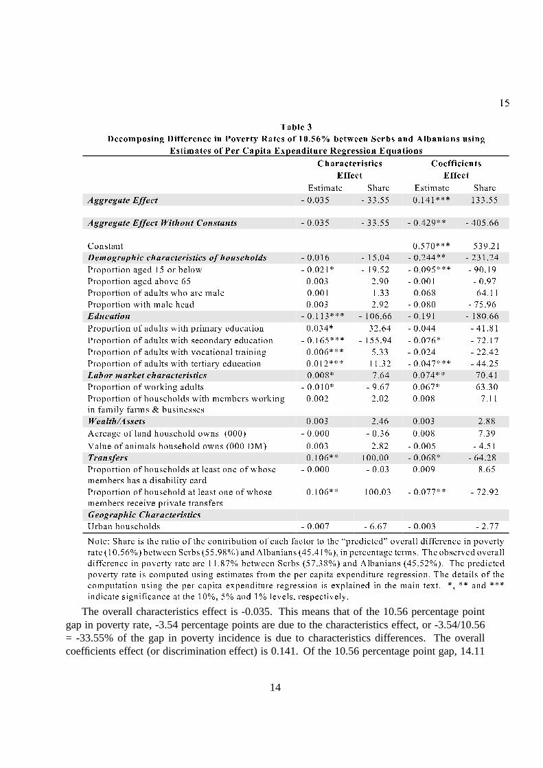
The overall characteristics effect is -0.035. This means that of the 10.56 percentage pointgap in poverty rate, -3.54 percentage points are due to the characteristics effect, or -3.54/10.56= -33.55% of the gap in poverty incidence is due to characteristics differences. The overallcoefficients effect (or discrimination effect) is 0.141. Ofthe 10.56 percentage point gap, 14.11

14

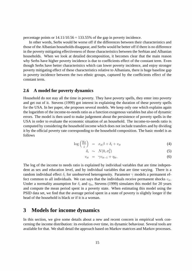
percentage points or 14.11/10.56 = 133.55% of the gap in poverty incidence.In other words, Serbs would be worse off if the differences between their characteristics and

those of the Albanian households disappear, and Serbs wouldbe better off if there is no differencein the poverty mitigating effectiveness of those characteristics between the Serbian and Albanianhouseholds. When we look at detailed decomposition, it becomes clear that the main reasonwhy Serbs have higher poverty incidence is due to coefficients effect of the constant term. Eventhough Serbs have better characteristics which can lower poverty incidence, and enjoy strongerpoverty mitigating effect of these characteristics relative to Albanians, there is huge baseline gapin poverty incidence between the two ethnic groups, captured by the coefficients effect of theconstant term.

2.6 A model for poverty dynamics

Household do not stay all the time in poverty. They have poverty spells, they enter into povertyand get out of it. Stevens (1999) got interest in explaining the duration of these poverty spellsfor the USA. In her paper, she proposes several models. We keep only one which explains againthe logarithm of the income-to-needs ratio as a function exogenous variables but also of dynamicerrors. The model is then used to make judgement about the persistence of poverty spells in theUSA in order to evaluate the economic situation of an household. The income-to-needs ratio iscomputed by considering the household income which does notinclude transfers and by dividingit by the official poverty rate corresponding to the household composition. The basic model is asfollows

log(yitz

)= xitβ + δi + vit (4)

δi ∼ N(0, σ2δ ) (5)

vit = γvit−1 + ηit. (6)

The log of the income to needs ratio is explained by individual variables that are time indepen-dent as sex and education level, and by individual variablesthat are time varying. There is arandom individual effectδi for unobserved heterogeneity. Parameterγ models a permanent ef-fect common to all individuals. We can says that the individuals receive permanent shocksvit.Under a normality assumption forδi andηit, Stevens (1999) simulates this model for 20 yearsand compute the mean period spent in a poverty state. When estimating this model using thePSID data set, we find that the average period spent in a state of poverty is slightly longer if thehead of the household is black or if it is a woman.

3 Models for income dynamics

In this section, we give some details about a new and recent concern in empirical work con-cerning the income distribution: its evolution over time, its dynamic behaviour. Several tools areavailable for that. We shall detail the approach based on Markov matrices and Markov processes.

15

In a first step we shall consider simple Markov matrices, detail the significance of income mo-bility and indicate how Markov matrices can be estimated. Wepropose some mobility indicestogether with their asymptotic distribution. We finally indicate how one can introduce explana-tory variables for explaining income mobility using a dynamic multinomial logit model.

3.1 Income dynamics

In his presidential address to the European Society for Population Economics, Jenkins (2000) un-derlines that the income distribution in the UK has experienced great changes during the eighties,but that since 1991, this distribution seems to have remained relatively stable. If the poverty lineis defined as half the mean income, the percentage of poor remains relatively stable, while if itis defined as half the mean of 1991 in real term, this percentage decreases steadily. The Ginicoefficient remains extremely stable around 0.31-0.32. These figures characterise a cross-sectionstability in income.

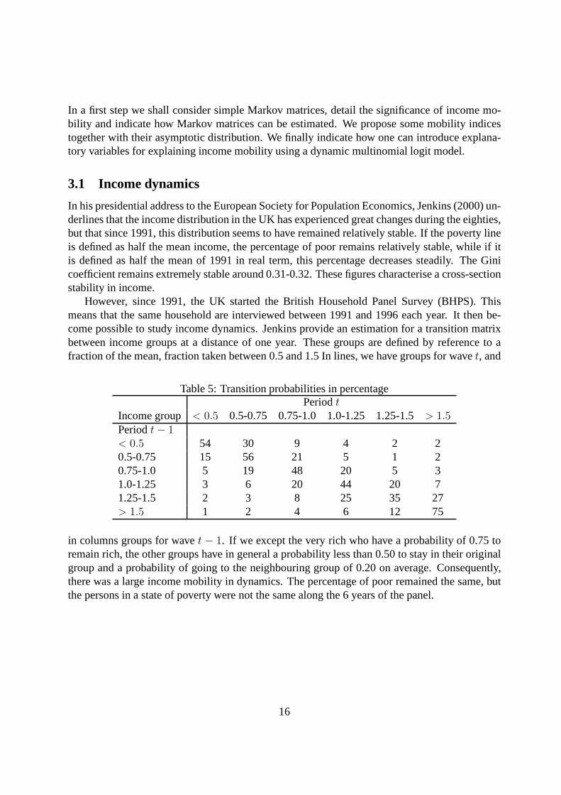
However, since 1991, the UK started the British Household Panel Survey (BHPS). Thismeans that the same household are interviewed between 1991 and 1996 each year. It then be-come possible to study income dynamics. Jenkins provide an estimation for a transition matrixbetween income groups at a distance of one year. These groupsare defined by reference to afraction of the mean, fraction taken between 0.5 and 1.5 In lines, we have groups for wavet, and

Table 5: Transition probabilities in percentagePeriodt

Income group < 0.5 0.5-0.75 0.75-1.0 1.0-1.25 1.25-1.5> 1.5Periodt− 1< 0.5 54 30 9 4 2 20.5-0.75 15 56 21 5 1 20.75-1.0 5 19 48 20 5 31.0-1.25 3 6 20 44 20 71.25-1.5 2 3 8 25 35 27> 1.5 1 2 4 6 12 75

in columns groups for wavet − 1. If we except the very rich who have a probability of 0.75 toremain rich, the other groups have in general a probability less than 0.50 to stay in their originalgroup and a probability of going to the neighbouring group of0.20 on average. Consequently,there was a large income mobility in dynamics. The percentage of poor remained the same, butthe persons in a state of poverty were not the same along the 6 years of the panel.

16

3.2 Transition matrices and Markov models

How was the previous transition matrix computed? It characterises social mobility, the passagebetween different social states over a given period of time.

- There arek different possible social states.

- i is the starting state,j the destination state

- pij is the probability to move from statei to statej during the reference period.

We are in fact introducing a Markov process of order one. It can be used to model

- changes in voting behaviour

- changes of social status between father and son: Prais (1955).

- change in occupational status

- change in geographical regions

- Income mobility between different income classes over oneor several years

Let us considerk different states (job status, occupational status, incomeclass, etc...) suchthat an individual is assigned to only one state at a given time period. We letnij , i, j = 1...k bethe number of individuals initially in statei moving to statej in the next period. We define

ni. =

k∑

j=1

nij

the initial number of people in statei andn =∑k

i=1 ni. the total number of individuals in thesample. We define a transition matrixP as a matrix with independent lines which sum up to one,P = [pij] wherepij represents the conditional probability for an individual to move from stateito statej in the next period. We have

∑j pij = 1.

Let us callπ(0) the row vector of probabilities of thek initial states at time 0. The row vectorof probabilities at time 1 is given byπ(1). The relation betweenπ(0) andπ(1) is given by

π(1) = π(0)P,

by definition of the transition matrix. From theStationarity Markov assumption we can derivethat the transition matrixP is constant over time such that the distribution at timet is given by

π(t) = π(0)P t.

We suppose that the transition matrix hask distinct eigenvalues|λ1| > |λ2| > .... > |λm|. SinceP is a row stochastic matrix, its largest left eigenvalue is 1.Consequently,P t is perfectly definedand converges to a finite matrix whent tends to infinity.

17

The stationary distributionπ∗ = (π∗1, ..., π

∗k)

∗ is a row vector of non negative elements whichsum up to 1 such that

π∗ = π∗P.

This distribution vector is a normalised (meaning that the sum of its entries is 1) left eigenvectorof the transition matrix associated with the eigenvalue 1. If the Markov chain is irreducible (it ispossible to get to any state from any state) and aperiodic (anindividual returns to statei can occurat irregular times), then there is a unique stationary distributionπ∗ and in this caseP t convergesto a rank-one matrix in which each row is the stationary distributionπ∗, that is

limt→∞P t =

π∗1 · · ·π∗

m

· · ·π∗1 · · ·π∗

m

= i

′π∗

with i being the unity column vector of dimensionk.Markov processes model the transition between mutually exclusive classes or states. In a

group of applications, mainly those coming from the sociological literature, those classes areeasy to define because they correspond to a somehow natural partition of the social space. Wehave for instance social classes, social prestige, voting behaviour or more simply economics jobstatus as working, unemployed, not working. In fact those social statuses are directly linked todichotomous variables. For studying income mobility, the problem is totaly different becauseincome is a continuous variable that has to be discretised. And there are dozen of ways ofdiscretising a continuous variable.

It is easier to detail the various aspects of Markov processes used to model social mobility, itis easier to start from the case where the classes are directly linked to a discrete variable. We shallinvestigate income mobility in a second step, detailing at that occasion the specific questions thatare raised by discretisation.

3.3 Building transition matrices

When considering income as a continuous random variable, there are several ways to build in-come classes. Let us start by considering a joint distribution between two income variablesx ∈ [0,∞) andy ∈ [0,∞) with a continuous joint cumulative distribution functionK(x, y) thatcaptures the correlation betweenx andy. These correlations may be intergenerational ifx is,say, the father andy the son or intra-generational ifx andy are the same sample income givenat two points in time. The marginal distribution ofx andy are denotedF (x) andG(y) suchthatF (x) = F (x,∞) andG(y) = G(∞, y). We assume thatF (.), G(.) andK(., .) are strictlymonotone and the first two moments ofx andy exist and are finite.

Form given income class boundaries0 < ζ1 < ... < ζm−1 < ∞ and0 < ξ1 < ... < ξm−1 <∞, we can derive the income transition matrixP related toK(x, y) such that each elementpijcould be written as

pij =Pr(ζi−1 ≤ x ≤ ζi andξj−1 ≤ y ≤ ξj)

Pr(ζi−1 ≤ x ≤ ζi), (7)

whereζ0 = ξ0 = 0 andζm = ξm = ∞.

18

Four approaches are recommended in Formby et al. (2004) to construct an income transitionmatrix.

The first oneconsiders class boundaries as defined exogenously. The resulting matrix isreferred as a size transition matrix. With this approach theclass boundaries do not depend on aparticular income regime or distribution. One major advantage of this method is that it reflectsincome movements between different income levels. Thus both the exchange of income positionsas well as the global income growth are taken into account. Intheir comparison of mobilitydynamics between the US and Germany during the eighties, Formby et al. (2004) set five earningclasses and normalised German earning using the US mean earnings to compare mobility in theUS to mobility in Germany. We shall see that, on average, there is more mobility in the US thanin Germany.

The second approachis recommended when mobility is considered as a relative concept andwe want to isolate the effects of global income growth from the effects of mobility. In thiscase mobility is considered as a re-ranking of individuals among income classes and we’ll usequantile transition matrices. The main advantage of this approach is that the transition matrixis bi-stochastic (

∑mi=1 pij =

∑mj=1 pij = 1) and the steady state condition is always satisfied.

Hungerford (1993) used quantile transition matrices to asses the changes in income mobility inthe US in the seventies and the eighties.

The third and fourth approachesinclude both elements of the absolute and relative ap-proaches to mobility. In fact, class boundaries are computed as percentages of the mean or themedian. The resulting matrices are referred as mean transition matrices and median transitionmatrices. Using British data from the BHPS waves 1-6, Jenkins (2000) estimates mean transitionmatrices to show the importance of income mobility in the UK society. We have reproduced thatmatrix in the introduction of this section.

3.4 What is social mobility: Prais (1955)

According to Bartholomew (1982), Prais (1955) was the first paper in economics to study socialmobility using a Markov model (see Feller 1950, chap 15, or Feller 1968 for a theory of Markovprocesses). Prais (1955) considered a random sample of 3500males aged over 18 from the SocialSurvey in 1949. He studied mobility between father and son and produced the following Markovtransition matrix reproduced in Table 6. The equilibrium distribution is given by

π′∗ = π′

∗P.

Once this distribution is reached, it will be kept for ever. Thus the equilibrium distribution isindependent of the starting distribution. It is also independent of the time span. As ifP relatesthe status of sons to that of fathers, the matrix relating that of grandsons to grandfathers isP 2.

There is perfect immobility if a family always stays in the same class. This would correspondtoP = I. The more mobile is a family, the shorter the period it would stay in the same class.

Let us callnj the number of families in classj at the beginning of the period. In the secondgeneration, there will benjpjj, thennjp

2jj and so on. The average time (measured in number of

19

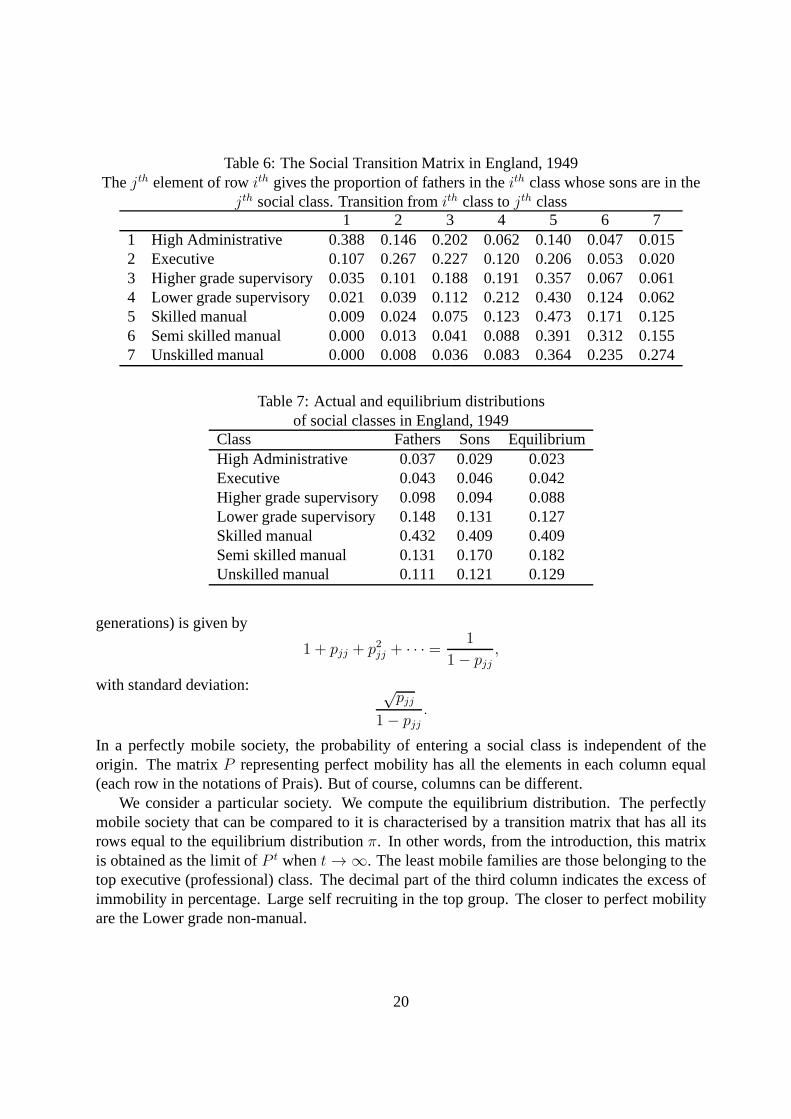
Table 6: The Social Transition Matrix in England, 1949Thejth element of rowith gives the proportion of fathers in theith class whose sons are in the

jth social class. Transition fromith class tojth class1 2 3 4 5 6 7

1 High Administrative 0.388 0.146 0.202 0.062 0.140 0.047 0.0152 Executive 0.107 0.267 0.227 0.120 0.206 0.053 0.0203 Higher grade supervisory 0.035 0.101 0.188 0.191 0.357 0.067 0.0614 Lower grade supervisory 0.021 0.039 0.112 0.212 0.430 0.124 0.0625 Skilled manual 0.009 0.024 0.075 0.123 0.473 0.171 0.1256 Semi skilled manual 0.000 0.013 0.041 0.088 0.391 0.312 0.1557 Unskilled manual 0.000 0.008 0.036 0.083 0.364 0.235 0.274

Table 7: Actual and equilibrium distributionsof social classes in England, 1949

Class Fathers Sons EquilibriumHigh Administrative 0.037 0.029 0.023Executive 0.043 0.046 0.042Higher grade supervisory 0.098 0.094 0.088Lower grade supervisory 0.148 0.131 0.127Skilled manual 0.432 0.409 0.409Semi skilled manual 0.131 0.170 0.182Unskilled manual 0.111 0.121 0.129

generations) is given by

1 + pjj + p2jj + · · · = 1

1− pjj,

with standard deviation: √pjj

1− pjj.

In a perfectly mobile society, the probability of entering asocial class is independent of theorigin. The matrixP representing perfect mobility has all the elements in each column equal(each row in the notations of Prais). But of course, columns can be different.

We consider a particular society. We compute the equilibrium distribution. The perfectlymobile society that can be compared to it is characterised bya transition matrix that has all itsrows equal to the equilibrium distributionπ. In other words, from the introduction, this matrixis obtained as the limit ofP t whent → ∞. The least mobile families are those belonging to thetop executive (professional) class. The decimal part of thethird column indicates the excess ofimmobility in percentage. Large self recruiting in the top group. The closer to perfect mobilityare the Lower grade non-manual.

20

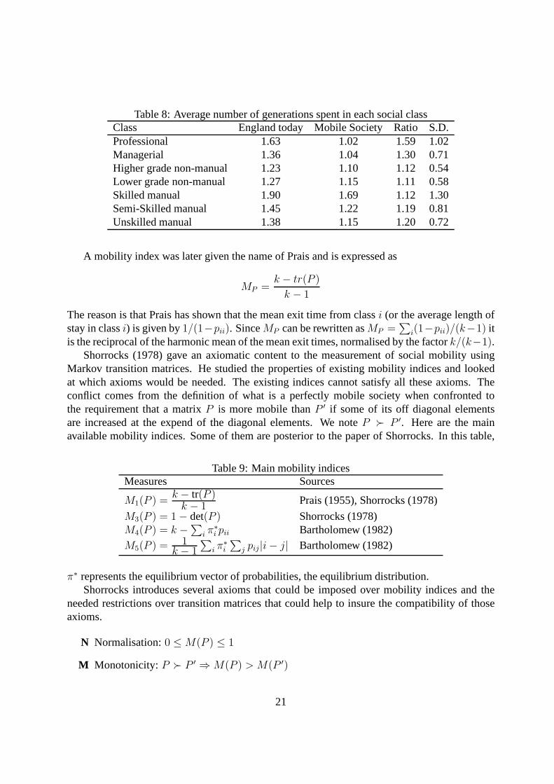
Table 8: Average number of generations spent in each social classClass England today Mobile Society Ratio S.D.Professional 1.63 1.02 1.59 1.02Managerial 1.36 1.04 1.30 0.71Higher grade non-manual 1.23 1.10 1.12 0.54Lower grade non-manual 1.27 1.15 1.11 0.58Skilled manual 1.90 1.69 1.12 1.30Semi-Skilled manual 1.45 1.22 1.19 0.81Unskilled manual 1.38 1.15 1.20 0.72

A mobility index was later given the name of Prais and is expressed as

MP =k − tr(P )

k − 1

The reason is that Prais has shown that the mean exit time fromclassi (or the average length ofstay in classi) is given by1/(1−pii). SinceMP can be rewritten asMP =

∑i(1−pii)/(k−1) it

is the reciprocal of the harmonic mean of the mean exit times,normalised by the factork/(k−1).Shorrocks (1978) gave an axiomatic content to the measurement of social mobility using

Markov transition matrices. He studied the properties of existing mobility indices and lookedat which axioms would be needed. The existing indices cannotsatisfy all these axioms. Theconflict comes from the definition of what is a perfectly mobile society when confronted tothe requirement that a matrixP is more mobile thanP ′ if some of its off diagonal elementsare increased at the expend of the diagonal elements. We noteP � P ′. Here are the mainavailable mobility indices. Some of them are posterior to the paper of Shorrocks. In this table,

Table 9: Main mobility indicesMeasures Sources

M1(P ) =k − tr(P )k − 1

Prais (1955), Shorrocks (1978)

M3(P ) = 1− det(P ) Shorrocks (1978)M4(P ) = k −

∑i π

∗i pii Bartholomew (1982)

M5(P ) = 1k − 1

∑i π

∗i

∑j pij|i− j| Bartholomew (1982)

π∗ represents the equilibrium vector of probabilities, the equilibrium distribution.Shorrocks introduces several axioms that could be imposed over mobility indices and the

needed restrictions over transition matrices that could help to insure the compatibility of thoseaxioms.

N Normalisation:0 ≤ M(P ) ≤ 1

M Monotonicity:P � P ′ ⇒ M(P ) > M(P ′)

21

I Immobility: M(I) = 0

SI Immobility: M(I) = 0 iff P = I

PM Perfect mobility:M(P ) = 1 if P = i′x with x′i = 1.

The index of Bartholomew satisfies (I ) but not (SI), (N), (M ), or (PM). The reason is that theaxioms (N), (M ), and (PM) are incompatible. The basic conflict is thus between (PM) and (M ).This conflict can be removed reasonably by considering transition matrices that are maximaldiagonal

pii > pij , ∀i, jor quasi maximal diagonal

µipii > µjpij , ∀i, j andµi, µj > 0.

With this last restriction, the Prais index satisfies (I), (SI), and (M).

3.5 Estimating transition matrices

Each row of a transition matrixP defines a multinomial process which is independent of theother rows. Anderson and Goodman (1957) or Boudon (1973, pages146-149) among othersproved that the maximum likelihood estimator of each element of P is

P = [pij ] =

[nij

ni

].

This estimatorpij is consistent and has variance

nipij(1− pij)/n2i = pij(1− pij)/ni.

Whenn tends to infinity, each rowPi of P tends to a multivariate normal distribution with√ni(Pi − Pi)

D−→ N(0,Σi),

where

Σi =

pi1(1− pi1)ni

· · · −pi1pikni

. . .

−pikpi1ni

· · · pik(1− pik)ni

.

As each row of matrixP is independent of the others, the stacked vector of the rowsPi verifies:√n(vec(P )− vec(P ))

D−→ N(0,Σ),

where

Σ =

Σ1 · · · 0

0. . .

0 · · · Σk

(8)

is ak2 × k2 block diagonal matrix withΣi on its diagonal and zeros elsewhere.

22

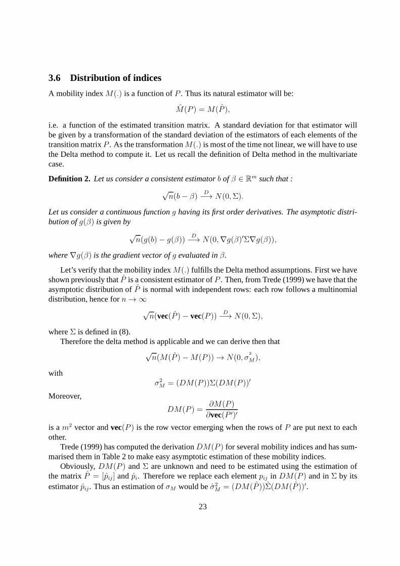
3.6 Distribution of indices

A mobility indexM(.) is a function ofP . Thus its natural estimator will be:

M(P ) = M(P ),

i.e. a function of the estimated transition matrix. A standard deviation for that estimator willbe given by a transformation of the standard deviation of theestimators of each elements of thetransition matrixP . As the transformationM(.) is most of the time not linear, we will have to usethe Delta method to compute it. Let us recall the definition ofDelta method in the multivariatecase.

Definition 2. Let us consider a consistent estimatorb of β ∈ Rm such that :

√n(b− β)

D−→ N(0,Σ).

Let us consider a continuous functiong having its first order derivatives. The asymptotic distri-bution ofg(β) is given by

√n(g(b)− g(β))

D−→ N(0,∇g(β)′Σ∇g(β)),

where∇g(β) is the gradient vector ofg evaluated inβ.

Let’s verify that the mobility indexM(.) fulfills the Delta method assumptions. First we haveshown previously thatP is a consistent estimator ofP . Then, from Trede (1999) we have that theasymptotic distribution ofP is normal with independent rows: each row follows a multinomialdistribution, hence forn → ∞

√n(vec(P )− vec(P ))

D−→ N(0,Σ),

whereΣ is defined in (8).Therefore the delta method is applicable and we can derive then that

√n(M(P )−M(P )) → N(0, σ

2

M ),

withσ2M = (DM(P ))Σ(DM(P ))′

Moreover,

DM(P ) =∂M(P )

∂vec(P ′)′

is am2 vector andvec(P ) is the row vector emerging when the rows ofP are put next to eachother.

Trede (1999) has computed the derivationDM(P ) for several mobility indices and has sum-marised them in Table 2 to make easy asymptotic estimation ofthese mobility indices.

Obviously,DM(P ) andΣ are unknown and need to be estimated using the estimation ofthe matrixP = [pij] andpi. Therefore we replace each elementpij in DM(P ) and inΣ by itsestimatorpij. Thus an estimation ofσM would beσ2

M = (DM(P ))Σ(DM(P ))′.

23

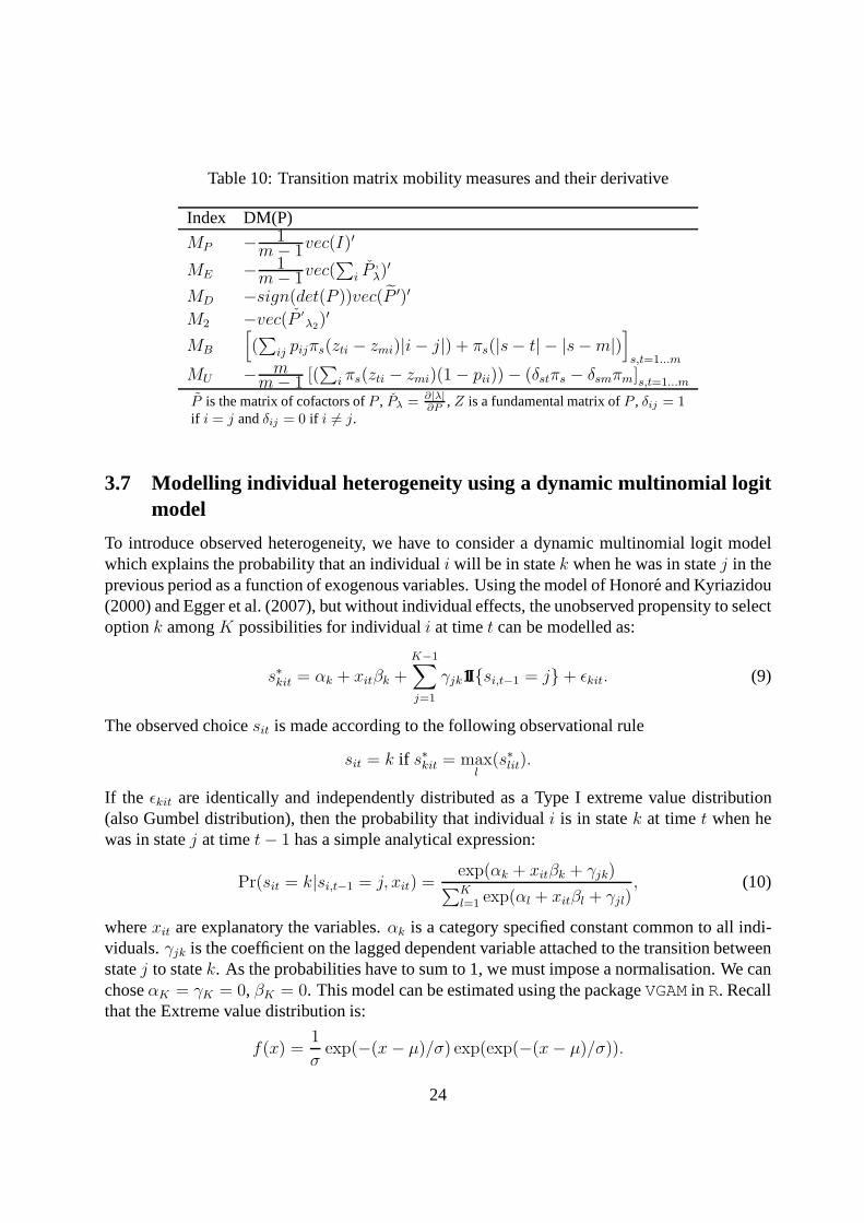
Table 10: Transition matrix mobility measures and their derivative

Index DM(P)

MP − 1m− 1vec(I)

′

ME − 1m− 1vec(

∑i P

,λ)

′

MD −sign(det(P ))vec(P ′)′

M2 −vec(P ′

λ2)′

MB

[(∑

ij pijπs(zti − zmi)|i− j|) + πs(|s− t| − |s−m|)]

s,t=1...m

MU − mm− 1 [(

∑i πs(zti − zmi)(1− pii))− (δstπs − δsmπm]s,t=1...m

P is the matrix of cofactors ofP , Pλ =∂|λ|∂P

, Z is a fundamental matrix ofP , δij = 1

if i = j andδij = 0 if i 6= j.

3.7 Modelling individual heterogeneity using a dynamic multinomial logitmodel

To introduce observed heterogeneity, we have to consider a dynamic multinomial logit modelwhich explains the probability that an individuali will be in statek when he was in statej in theprevious period as a function of exogenous variables. Usingthe model of Honore and Kyriazidou(2000) and Egger et al. (2007), but without individual effects, the unobserved propensity to selectoptionk amongK possibilities for individuali at timet can be modelled as:

s∗kit = αk + xitβk +K−1∑

j=1

γjk1I{si,t−1 = j}+ εkit. (9)

The observed choicesit is made according to the following observational rule

sit = k if s∗kit = maxl

(s∗lit).

If the εkit are identically and independently distributed as a Type I extreme value distribution(also Gumbel distribution), then the probability that individual i is in statek at timet when hewas in statej at timet− 1 has a simple analytical expression:

Pr(sit = k|si,t−1 = j, xit) =exp(αk + xitβk + γjk)∑Kl=1 exp(αl + xitβl + γjl)

, (10)

wherexit are explanatory the variables.αk is a category specified constant common to all indi-viduals.γjk is the coefficient on the lagged dependent variable attachedto the transition betweenstatej to statek. As the probabilities have to sum to 1, we must impose a normalisation. We canchoseαK = γK = 0, βK = 0. This model can be estimated using the packageVGAMin R. Recallthat the Extreme value distribution is:

f(x) =1

σexp(−(x− µ)/σ) exp(exp(−(x− µ)/σ)).

24

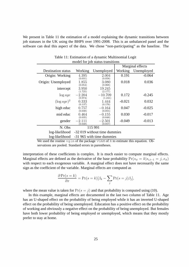
We present in Table 11 the estimation of a model explaining the dynamic transitions betweenjob statuses in the UK using the BHPS over 1991-2008. This is an unbalanced panel and thesoftware can deal this aspect of the data. We chose “non-participating” as the baseline. The

Table 11: Estimation of a dynamic Multinomial Logitmodel for job status transitions

Marginal effectsDestination status Working UnemployedWorking UnemployedOrigin: Working 4.395

(0.031)2.004(0.058)

0.191 -0.064

Origin: Unemployed 1.855(0.054)

3.080(0.068)

0.018 0.036

intercept 3.950(1.725)

19.245(2.177)

log age −2.204(0.974)

−10.709(1.241)

0.172 -0.245

(log age)2 0.333(0.137)

1.444(0.176)

-0.021 0.032

high educ 0.757(0.038)

−0.164(0.055)

0.047 -0.025

mid educ 0.464(0.035)

−0.155(0.048)

0.030 -0.017

gender −2.111(0.048)

−2.501(0.057)

-0.049 -0.013

N. Obs 115 991log-likelihood -32 019 without time dummieslog-likelihood -31 965 with time dummies

We used the routinevglm of the packageVGAMof R to estimate this equation. Ob-servations are pooled. Standard errors in parentheses.

interpretation of these coefficients is complex. It is much easier to compute marginal effects.Marginal effects are defined as the derivative of the base probability Pr(sit = k|si,t−1 = j, xit)with respect to each exogenous variable. A marginal effect does not have necessarily the samesign as the coefficient of the variable. Marginal effects arecomputed as

∂ Pr(s = k)

∂x= Pr(s = k)[βk −

∑

j

Pr(s = j)βj],

where the mean value is taken forPr(s = j) and that probability is computed using (10).In this example, marginal effects are documented in the lasttwo column of Table 11. Age

has an U-shaped effect on the probability of being employed while it has an inverted U-shapedeffect on the probability of being unemployed. Education has a positive effect on the probabilityof working and obviously a negative effect on the probability of being unemployed. But femaleshave both lower probability of being employed or unemployed, which means that they mostlyprefer to stay at home.

25

3.8 Transition matrices and individual probabilities

A Markov transition matrix is usually estimated by maximum likelihood which is shown tocorrespond to (see the seminal paper of Anderson and Goodman1957 or the appendix in Boudon1973):

pij(t) =nij(t)∑j nij(t)

,

wherenij(t) the number of individuals in statei at timet− 1 moving to statej at timet. Whenthere are more than two periods and if the process is homogenous, the maximum likelihoodestimator is obtained by averaging theptij obtained between two consecutive periods. Of course,this estimator is not at ease when the panel is incomplete.

The dynamic multinomial logit model can be seen as an alternative to estimate a Markovtransition matrix. We can exploit the conditional probabilities given (10) that we recall here

Pr(sit = k|si,t−1 = j, xit) =exp(αk + xitβk + γjk)∑Kl=1 exp(αl + xitβl + γjl)

,

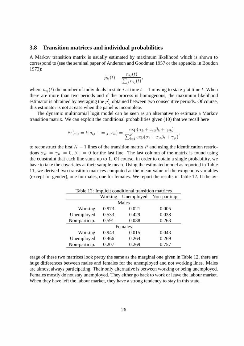
to reconstruct the firstK − 1 lines of the transition matrixP and using the identification restric-tionsαK = γK = 0, βK = 0 for the last line. The last column of the matrix is found usingthe constraint that each line sums up to 1. Of course, in orderto obtain a single probability, wehave to take the covariates at their sample mean. Using the estimated model as reported in Table11, we derived two transition matrices computed at the mean value of the exogenous variables(except for gender), one for males, one for females. We report the results in Table 12. If the av-

Table 12: Implicit conditional transition matricesWorking Unemployed Non-particip.

MalesWorking 0.973 0.021 0.005

Unemployed 0.533 0.429 0.038Non-particip. 0.591 0.038 0.263

FemalesWorking 0.943 0.015 0.043

Unemployed 0.466 0.264 0.269Non-particip. 0.207 0.269 0.757

erage of these two matrices look pretty the same as the marginal one given in Table 12, there arehuge differences between males and females for the unemployed and not working lines. Malesare almost always participating. Their only alternative isbetween working or being unemployed.Females mostly do not stay unemployed. They either go back towork or leave the labour market.When they have left the labour market, they have a strong tendency to stay in this state.

26

4 Introducing and illustrating quantile regressions

A regression model gives the link, either linear or non-linear, that exists between an endogenousvariable and one or more exogenous variables. In the most simplest case, the regression linerepresents a linear conditional expectation. A non-parametric regression explains a conditionalexpectation in a non-linear way, without specifying a predefined non-linear relationship. Butnone of these regressions is designed to explain the quantiles of the conditional distribution ofthe endogenous variable. The quantile regression was introduced in econometrics by Koenkerand Basset (1978); it gives the adequate tool to explain the compete evolution of the conditionaldistribution of the endogenous variable. The basic principle of the quantile regression is simple,but its numerical implementation is more complex. In particular, standard deviations are not easyat all to compute. So most of the time, bootstrap is used to obtain numerical values.

4.1 Classical quantile regression

Let us consider a linear regression model expressed as

y = x′β + e.

In the usual linear regression the assumption is E(e|x) = 0. And no other special assumptionconsidering the distribution ofy is needed.

A quantile regression model considers a similar linear regression, but adds the fact that thisregression can be estimated for every predefined quantileτ of the endogenous variable. So fortheτ th quantile, we have now the new regression:

yi = x′iβτ + eiτ , (11)

where the parameter to be estimated are theβ′

τ = (β0τ , · · · , βkτ ). A coherent definition of thisregression requires no longer that E(ei|xi) = 0, but that theτ th quantile ofe is equal to zero. Iff(.) is the density ofe, this means that

∫ 0

−∞

fτ (ei|x)d ei = τ. (12)

In other words, if the distribution isF (.), let us noteqτ (x) the quantile of levelτ that we defineas

qτ (y) = F−1(τ).

A quantile regression explains this quantile by a linear combination of thex

qτ (y) = x′β.

We shall first note that ifF is a cumulative normal, this model will provide no valid new infor-mation, because first the mean and the median are identical for this distribution and second thatits conditional quantiles are straight lines. We have to getout of this traditional framework in

27

order to get a valid and interesting model. A first possibility is to have heteroscedastic errors, forinstance normal errors but with a non-constant varianceσ2

i ; for instance this last parameter canbe function of exogenous variables. A more radical assumption is simply to have distributionalrestriction forF and thus to use a semi-parametric framework. For this, we define the errorfunction

ρτ (u) =

{uτ if u > 0,u(τ − 1) if u ≤ 0.

We then look for the value ofβ that minimises, not a quadratic distance of the error term, but themore peculiar function

βτ = argmin∑

i

ρτ (yi − x′iβ).

This has to be solved using quadratic programming. This approach was first proposed by Koenkerand Basset (1978). It is very difficult to compute standard errors.

4.2 Bayesian inference

Other routes are possible to define a quantile regression. Using a Bayesian framework, Yu andMoyeed (2001) show that estimating the quantile ofy is equivalent to estimating the localisationparameter of an asymmetric Laplace distribution. This leads easily to writing the likelihoodfunction as:

Lτ (β; y, x) ∝ τn(1− τ)n exp{−∑

i

ρτ (yi − x′iβ)},

which is used by Yu and Moyeed (2001) to evaluate the posterior density ofβ. In this framework,it becomes easy to estimate standard deviations and computeconfidence intervals.

4.3 Quantile regression using R

There are several packages in R for computing quantile regressions. Different approaches arepossible.

The packagelibrary(quantreg) contains all the necessary tools for semi-parametricquantile regression. The basic command isrq . This package corresponds to the original methodof Koenker and Basset (1978).

For a fully non-parametric approach, we need the general packagelibrary(np) . Thenthe routine isnpqreg . There is an example using an Italian income panel which should beinvestigated seriously.

In a Bayesian approach, the package islibrary(MCMCpack) , and then we can useMCMCquantreg . The prior density forβ is normal. The quantile has to be given. By defaultτ = 0.5. There should be as many runs as quantiles needed.

28

4.4 Analysing poverty in Vietnam

Nguyen et al. (2007) use the Vietnam Living Standards Surveys from 1993 and 1998 to examineinequality in welfare between urban and rural areas in Vietnam. Their measure of welfare isthe log of real per capita household consumption expenditure (RPCE), presumably because it iseasier to have better data on consumption than on income. Their basic quantile regression forquantileτ is

qτ (y|x) = β0τ + x′βτ + urban(γ0

τ +Xγτ ) + south(δ0τ +Xδ0τ ) + urban× southθ0τ ,

wherey is the log of RPCE. They first run a regression with including only regional and urbandummies to highlight the differences. They will include theother explanatory variables lateron. The coefficients labelledbaseare estimates of log RPCE for the base case: a northern

Table 13: Estimates of the urban-rural gap at the meanand at various quantiles

OLS 5th 25th 50th 75th 95th1993 base 7.25 6.62 6.98 7.24 7.51 7.96

p-value (0.00) (0.00) (0.00) (0.00) (0.00) (0.00)urban 0.52 0.34 0.42 0.51 0.59 0.74

p-value (0.00) (0.00) (0.00) (0.00) (0.00) (0.00)south 0.20 -0.02 0.15 0.22 0.29 0.36

p-value (0.00) (0.83) (0.00) (0.00) (0.00) (0.00)1998 base 7.56 6.85 7.26 7.53 7.84 8.35

p-value (0.00) (0.00) (0.00) (0.00) (0.00) (0.00)urban 0.72 0.60 0.64 0.72 0.79 0.93

p-value (0.00) (0.00) (0.00) (0.00) (0.00) (0.00)south 0.15 -0.05 0.12 0.17 0.21 0.22

p-value (0.00) (0.54) (0.00) (0.00) (0.00) (0.00)Bootstrapped standard errors were computed on 1000 replications and accountfor the effects of clustering and stratification. The p-values are for two-sidedtests based on asymptotic standard normal distributions ofthe z-ratios underthe null hypothesis that the corresponding coefficients arezero.

rural household. There is an increased dispersion for the urban households. The quantiles arenot linear. The 95th quantile is much higher than expected. This dispersion is even increasedin 1998 compared to 1993. On the contrary, the dispersion between north and south is muchsmoother and tends to decrease over time. These differencesare significant for all the quantiles,except for the 5th which is not significant. Poverty is the same in both regions as the 5th quantilefor the dummy south is not significant.

When the model is estimated in full, including all covariates, the apparent advantages of thesouth shown in the Table 13 disappear. So the differences arefully explained by these covariates.

29

The increase in the rural-urban gap over the period (as shownin Table 13) is due to changes inthe distributions of the covariates and in changes in the returns of the covariates.

Nguyen et al. (2007) do not report in their main text the full regression, but simply commenton some covariates such as education. These comments are as follows:

Returns to education across the quantiles vary between the North and South. The returnsto education show a marked increase at the upper quantiles inthe South in 1993 for urbanhouseholds. A comparable pattern is not seen in the North. In1998, the upward sloping returnsto education in the South are evident in both the urban and rural sectors. The North in 1998continues to show a more stable pattern of returns across thequantiles with a huge blip up forthe very top urban households. Finally, returns to education increased, most substantially in theSouth, over the five-year period covered by our data.

The urban - rural gap is thus mainly due to differences in education for the smallest quantiles.However, for the higher quantiles of the income distribution, the rural - urban gap is mainly dueto differences in the yield of education. We can conclude that fighting against poverty goesthrough developing education in rural areas.

5 Marginal quantile regressions

In this section, we present another view of the quantile regression which was promoted by Firpoet al. (2009). Using a transformation of the endogenous variable, these authors manage to definea new concept of quantile regression, the marginal quantileregression, which proves to be veryuseful for computing an Oaxaca decomposition, which otherwise is quite difficult to define forthe usual conditional quantile regression. This section draws on Lubrano and Ndoye (2012).

5.1 Influence function

The Influence Function(IF ), first introduced by Hampel (1974), describes the influence of aninfinitesimal change in the distribution of a sample on a real-valued functional distribution orstatisticsν(F ), whereF is a cumulative distribution function. TheIF of the functionalν isdefined as

IF (y, ν, F ) = limε→0

ν(Fε,∆y)− ν(F )

ε=

∂ν(Fε,∆y)

∂ε|ε=0 (13)

whereFε,∆y= (1−ε)F + ε∆y is a mixture model with a perturbation distribution∆y which puts

a mass 1 at any pointy. The expectation ofIF is equal to 0.Firpo et al. (2009) make use of (13) by considering the distributional statisticsν(.) as the

quantile function(ν(F ) = qτ ) to find how a marginal quantile ofy can be modified by a smallchange in the distribution of the covariates. They make use of the RecenteredIF (RIF ), definedas the original statistics plus theIF so that the expectation of theRIF is equal to the originalstatistics.

Considering theτ th quantileqτ defined implicitly asτ =∫ qτ−∞

dF (y), Firpo et al. (2009)

30

show that theIF for the quantile of the distribution ofy is given by

IF (y, qτ(y), F ) =τ − 1I(y ≤ qτ )

f(qτ ),

wheref(qτ ) is the value of the density function ofy evaluated atqτ . The correspondingRIF issimply defined by

RIF (y, qτ , F ) = qτ +τ − 1I(y ≤ qτ )

f(qτ ), (14)

with the immediate property that

E (RIF (y, qτ)) =

∫RIF (y, qτ)f(y)dy = qτ .

5.2 Marginal quantile regression

The illuminating idea of Firpo et al. (2009) is to regress theRIF on covariates, so the change inthe marginal quantileqτ is going to be explained by a change in the distribution of thecovariatesby means of a simple linear regression:

E[RIF (y, qτ |X)] = Xβ + ε. (15)

They propose different estimation methods: a standard OLS regression (RIF-OLS), a logit re-gression (RIF-Logit) and a nonparametric logit regression. The estimates of the coefficients ofthe unconditional quantile regressions,βτ obtained by a simple Ordinary Least Square (OLS)regression (RIF-OLS) are as follows:

βτ = (X ′X)−1

X ′RIF (y; qτ). (16)

The practical problem to solve is that theRIF depends on the marginal density ofy. Firpo et al.(2009) propose to use a non-parametric estimator for the density and the sample quantile forqτso that an estimate of theRIF for each observation is given by

RIF (yi; qτ ) = qτ +τ − 1I(y ≤ qτ )

f(qτ ).

Standard deviations of the coefficients are given by the standard deviations of the regression. InLubrano and Ndoye (2012), we propose a Bayesian approach to this problem where the marginaldensity ofy is estimated using a parametric mixture of densities.

References

Anderson, T. W. and Goodman, L. A. (1957). Statistical inference about Markov chains.TheAnnals of Mathematical Statistics, 28(1):89–110.

31

Atkinson, A. (2003). Income inequality in oecd countries: Data and explanations. WorkingPaper 49: 479–513, CESifo Economic Studies, CESifo.

Bailar, B. A. . (1991). Salary survey of u.s. colleges and universities offering degrees in statistics.Amstat News, 182:3–10.

Bartholomew, D. (1982).Stochastic Models for Social Processes. Wiley, London, 3rd edition.

Bauwens, L., Lubrano, M., and Richard, J.-F. (1999).Bayesian Inference in Dynamic Econo-metric Models. Oxford University Press, Oxford.

Bazen, S. and Joutard, X. (2013). The Taylor decomposition:A unified generalization of theOaxaca method to nonlinear models. Technical report, AMSE.

Bhaumik, S. K., Gang, I. N., and Yun, M.-S. (2006a). A note on decomposing differences inpoverty incidence using regression estimates: Algorithm and example. Working Paper 2006-33, Department of Economics, Rutgers University, Rutgers University.

Bhaumik, S. K., Gang, I. N., and Yun, M.-S. (2006b). A note on decomposing differences inpoverty incidence using regression estimates: Algorithm and example. Discussion Paper No.2262, IZA, Bonn, Germany. Available at SSRN: http://ssrn.com/abstract=928808.

Blinder, A. S. (1973). Wage discrimination: Reduced form and structural estimates.The Journalof Human Resources, 8(4):436–455.

Boudon, R. (1973).Mathematical Structures of Social Mobility. Elsevier, Amsterdam.

Bourguignon, F., Ferreira, F. H. G., and Leite, P. G. (2008).Beyond oaxaca-blinder: Accountingfor differences in household income distributions.Journal of Economic Inequality, 6(2):117–148.

Cowell, F. (1995).Measuring Inequality. LSE Handbooks on Economics Series. Prentice Hall,London.

Egger, P., Pfaffermayr, M., and Weber, A. (2007). Sectoral adjustment of employment to shiftsin outsourcing and trade: evidence from a dynamic fixed effects multinomial logit model.Journal of Applied Econometrics, 22(3):559–580.

Feller, W. (1968).An Introduction to Probability Theory and Its Applications. Wiley Series inProbability and Statistics. Wiley and Sons, New-York, 3rd edition.

Fergusson, T. S. (1967).Mathematical Statistics: a decision theoretic approach. AcademicPress, New York.

Firpo, S., Fortin, N. M., and Lemieux, T. (2009). Unconditional quantile regressions.Economet-rica, 77(3):953–973.

32

Formby, J. P., Smith, W. J., and Zheng, B. (2004). Mobility measurement,transition matrices andstatistical inference.Journal of Econometrics, 120:181–205.

Foster, J., Greer, J., and Thorbecke, E. (1984). A class of decomposable poverty measures.Econometrica, 52:761–765.

Hampel, F. R. (1974). The influence curve and its role in robust estimation. Journal of theAmerican Statistical Association, 69(346):383–393.

Hlavac, M. (2014). oaxaca: Blinder-Oaxaca decomposition in R. Technical report, HarvardUniversity.

Honore, B. E. and Kyriazidou, E. (2000). Panel data discrete choice models with lagged depen-dent variables.Econometrica, 68(4):839–874.

Hungerford, T. L. (1993). U.S. income mobility in the seventies and eighties.Review of Incomeand Wealth, 31(4):403–417.

Jann, B. (2008). The blinder-oaxaca decomposition for linear regression models.The StataJournal, 8(4):453–479. Standard errors for the Blinder-Oaxaca decomposition. Handout forthe 3rd German Stata Users Group Meeting, Berlin, April 8 2005.

Jenkins, S. P. (2000). Modelling household income dynamics. Journal of Population Economics,13:529–567.

Juhn, C., Murphy, K. M., and Pierce, B. (1993). Wage inequality and the rise in returns to skill.The Journal of Political Economy, 101(3):410–442.

Koenker, R. and Basset, G. (1978). Regression quantiles.Econometrica, 46(1):33–50.

Lubrano, M. and Ndoye, A. J. (2012). Bayesian unconditionalquantile regression: An analysisof recent expansions in wage structure and earnings inequality in the u.s. 1992-2009. Technicalreport, GREQAM.

Nguyen, B. T., Albrecht, J. W., Vroman, S. B., and Westbrook,M. D. (2007). A quantile regres-sion decomposition of urban–rural inequality in vietnam.Journal of Development Economics,83(2):466–490.

Oaxaca, R. (1973). Male-female wage differentials in urbanlabor markets.International Eco-nomic Review, 14:693–709.

Prais, S. J. (1955). Measuring social mobility.Journal of the Royal Statistical Society, Series A,Part I, 118(1):56–66.

Radchenko, S. I. and Yun, M.-S. (2003). A bayesian approach to decomposing wage differentials.Economics Letters, 78(3):431–436.

Shorrocks, A. F. (1978). The measurement of mobility.Econometrica, 46(5):1013–1024.

33

Shorrocks, A. F. (1980). The class of additively decomposable inequality measures.Economet-rica, 48(3):613–625.

Stevens, A. H. (1999). Climbing out of poverty, falling backin. The Journal of HumanRessources, 34(3):557–588.

Trede, M. (1998). Making mobility visible: a graphical device. Economics Letters, 59:77–82.

Trede, M. (1999). Statistical inference for measures of income mobility.Jahrbucher fur Nation-aloknomie und Statistik, 218:473–490.

Yu, K. and Moyeed, R. A. (2001). Bayesian quantile regression. Statistics and ProbabilityLetters, 54:437–447.

Yun, M.-S. (2004). Decomposing differences in the first moment. Economics Letters, 82(2):275–280.

6 Appendix

A Quantile regressions in full

A.1 Introduction

Considerons un echantillon d’une variable aleatoireY et sa densitef(y). On va definir lamoyenne comme

µ =

∫yf(y)dy

Si F (.) est la distribution deY , alors la mediane sera

q0.50(y) = F−1y (0.50)

On peut definir de la meme maniere les autres quantiles.

Considerons maintenant un echantillon bivarie de deux variables aleatoiresY et X dis-tribues conjointement selonf(y, x). Si f(y|x) est la distribution conditionnelle dey si x, alorsl’esperance conditionnelle E(y|x) se definit comme

E(y|x) =∫

yf(y|x)dy

qui va prendre autant de valeurs differentes quex. Il s’agit donc d’une fonction. SiF (.) est la dis-tribution Normale de moyenne(µy, µx) et de varianceσ2

y , σyx, σ2x, alors la fonction de regression

se note simplement par proprietes de Normale bivariee

E(y|x) = µy +σyx

σ2x

(x− µx).

34

On exprime donc l’esperance conditionnelle comme une fonction lineaire dex. Si l’on s’interessemaintenant aux quantiles conditionnels dans cette meme normale

qp(x) = µy +σyx

σ2x

(x− µx) + Φ−1(p)

√

σ2y −

σ2x,y

σ2x

.

Le cas de la Normale est tres particulier carq0.50(x) = E(y|x) et les autres fonctions quan-tiles sont des droites paralleles etant donne queΦ−1(0.50) = 0. Le quantile conditionnel est lamoyenne conditionnelle corrigee par la valeur du quantilede la normale standardisee multipliepar la racine carree de la variance conditionnelle.

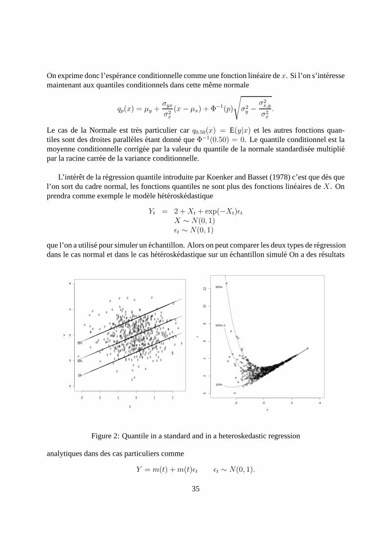
L’interet de la regression quantile introduite par Koenker and Basset (1978) c’est que des quel’on sort du cadre normal, les fonctions quantiles ne sont plus des fonctions lineaires deX. Onprendra comme exemple le modele heteroskedastique

Yt = 2 +Xt + exp(−Xt)εtX ∼ N(0, 1)εt ∼ N(0, 1)

que l’on a utilise pour simuler un echantillon. Alors on peut comparer les deux types de regressiondans le cas normal et dans le cas heteroskedastique sur unechantillon simule On a des resultats

o

o

oo

o

o

o

o

o

o

o

o

oo

oo

o

o oo

o

o

o

o

o

oo

o

o

o

o o

o

o o

o

o

o

o

oo

o

o

o

o

oo

o o

o

o

oo

o

o

o

o

o

o

o

o o

o

o

oo

o

oo

o

o

o

o

o

o

oo

oo

o

o

o

o

o

o

o

oo

oo

o

o

o

o

o

o

o

o

oo o

o

o

o

o

oo

o

o

o

oo

o

o

o o

o

o

oo

o

o

o

oo

o

o o

o

oo oo

o

o

o

o

o

o

o

o

o

o

o oo

oo

o

o

o

o

o

oo

o

o

o

o

o

o

o

o

o

oo

o

o

o

o

o

oo

o

oo

o

o

oo

o

o

o

o

o

o

o

o

o

o

o

o

oo

o

o

oo

o

o

oo

o

o

oo

o

o

o

o

o

o

o

o

o

o

o

o

o

o

o

o

o

o

o

oo

o

o

o

o

o

o o

o

oo

o

o

oo

oo

o

o

o o

o

o o

o

o

o

o

oo

o

ooo

o

o

oo

o

o

o

o

o

o

o

o

o

o

o

o

o

o

oo

oo o

o

o

o

o

oo

oo

oo o

o

o

o

o

o

o

o

o

oo

oo

o

oo

o

o

o

o

o

o

o

o

oo

o

o

o

o o

oo

o

o

o

o

o

o

oo

o

oo

o

o

o

oo o

o

oo

o

o

o

o oo

o

o

o

oo o

o

o

o

o

o

ooo

o

oo

o

o

oo

o

o

oo

o

o

o

o

o

o

o oo

o

o

o

o

o

o oo

o

o

oo

o

oo

o

o

o

o

o

o

o

o

o

o

o

o

o

o

o

oo

o

o

o

o

o

oo

oo

oo

o

o

oo

o

o

o

oo

o

o

oo

o

o

o

o

o

o

o

o

o

o

o

o

oo

o

o

o

o

o

o

oo

o

o

oo

o

o

o

o

o

o

ooo

o

o

oooo

o

o

oo

o

o

oo

o

o

o

o o

oo

oo

X

Y

-3 -2 -1 0 1 2

-4-2

02

4

5%

50%

95%

�������

�� ���

��� ����

�����

����

�� ��� ��

����

������

����� �� �� � ��

� ���

���

� �� ���

�� �����!�

� � �� ��� � ����

"#$#%�& �'"#$% �& ����"#$

( % �& �)

*+

o oo

o

o

oo

o

o

o

oo

o

o

o

o

o

o

o

oo

ooo

o

o o

oo

o

oo

ooo

oo

o

o

o

o

o o

o

oo

o ooo

o

o

o

ooo

oo

oo

o

oo

o

o

o

o

o

oo

oo

o

oo o

o

o

o

o o

o

oo

oo

oo

o

o

o oo

o

o

o

oo

oo

ooo

o

o

o

o

ooo

o

oo o

oo o

o

o

oo

oo

oo

o

o

o

o

ooo o

o

o

o

oo

o

o

o oo

o

o

oo

oooo

o

oo o

o

o

o

o

o

o

o

o

o

oo

o

o

o

o o

o

oo

o

o

o

oo

o

o oo

oo o

o o

o

o

o

o

o

o

o

o

o

oo

o

o

o

o

oo

oo

o

oo

o

o

o

o

o

o

o oo

o

o

o

o

o

o

o

o

oo

o

oo o

o

o o

o

o

o

oo

ooooo

o

o

ooo

o

o

o

o oo

o

oo

o

o

o

o

o

o

o

o

ooo

o

o o

o

o

o

oo

o

ooo

o

oo

oo

o

oo

o

oo

o

o

o

o

o

oo

o

ooo o

o

oo

o

o

o

o

o

o

o

o o

o

o

oo

oo

o

o

o

o

ooo

o

o

o

o

o

o

o

o

o

o oo

o

oo

o

o

o

o

o

o

o

o

oo

o

oo

o o

o

oo

oo

o

o

o

ooo

o

o

o

o

o

oo o

oo

oo

o

o

o o

o

o

o

o

oo

o

o

oo

o oo

oo

o

oo

o

oo o o

o

oo

o

o

o

oo o

o

oo

o

o

o

oo

o

o

o o

ooo

o

o

oo

oo

o

o

o

ooo

o

o

oo

o

o

o

o

oo

o

ooo

ooo

o

o

oo

o

oo

ooo o

o

o

o o o

o

o

o

o

oo

o

ooo

o

o

o

o o

o

o

o

o

o

x

y

-2 0 2 4

02

46

810

12

10%

50%

90%

�� � � � � � �� � � � � � �� � � � � � � � � � � � � � � � � � � � � � � � � � � ! � " � # � � � � ! � " � $ � � �� % � # � � � & �� ' �( � � � � ) � ! * "� ! * + # ! * , � � (� � � #

-!Figure 2: Quantile in a standard and in a heteroskedastic regression

analytiques dans des cas particuliers comme

Y = m(t) +m(t)εt εt ∼ N(0, 1).

35

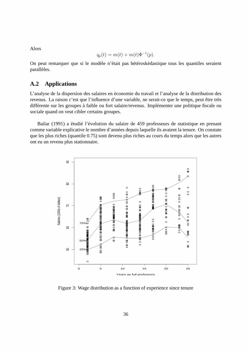
Alorsqp(t) = m(t) +m(t)Φ−1(p).

On peut remarquer que si le modele n’etait pas heterosk´edastique tous les quantiles seraientparalleles.

A.2 Applications

L’analyse de la dispersion des salaires en economie du travail et l’analyse de la distribution desrevenus. La raison c’est que l’influence d’une variable, ne serait-ce que le temps, peut etre tresdifferente sur les groupes a faible ou fort salaire/revenus. Implementer une politique fiscale ousociale quand on veut cibler certains groupes.

Bailar (1991) a etudie l’evolution du salaire de 459 professeurs de statistique en prenantcomme variable explicative le nombre d’annees depuis laquelle ils avaient la tenure. On constateque les plus riches (quantile 0.75) sont devenu plus riches au cours du temps alors que les autresont eu un revenu plus stationnaire.

o

oo

oo

o

o

o

oo

o

o

oo

o

o

o

o

o

o

o

o

o

o

o

o

o

o

o

oo

o

o

o

o

o

oo

o

o

o

ooooo

o

o

ooo

oooo

oo

o

o

o

oo

o

o

o

o

ooo

ooo

o

oo

o

o

o

o

oo

o

o

o

o

o

oo

o

o

o

o

o

o

o

o

o

o

o

o

o

oo

o

o

o

o

oo

o

o

o

o

oo

oo

o

oo

oo

o

o

o

oo

oo

oo

oo

o

o

oo

o

o

oo

o

o

oo

o

o

o

oo

o

o

o

o

o

o

ooo

o

o

oooo

o

o

o

o

o

o

o

o

oo

o

o

oo

o

o

o

o

o

o

o

o

o

oo

o

o

o

o

o

o

o

o

o

o

o

o

o

o

o

o

o

o

o

o

o

o

o

o

o

o

o

o

o

o

o

o

o

oo

o

oo

o

o

o

o

ooo

o

o

o

o

o

o

oo

o

o

o

oo

o

o

o

o

o

o

o

o

o

oo

o

o

o

oo

o

o

o

o

o

o

o

o

o

o

o

o

o

o

o

o

o

o

o

o

o

o

oo

o

oo

oo

o

o

o

o

oo

oo

oo

o

oo

oo

oo

o

o

o

o

o

o

oo

o

oo

o

o

o

ooo

o

o

o

o

oo

ooo

o

o

o

o

o

o

o

o

o

oo

o

o

o

oo

o

o

o

o

o

o

oo

o

o

o

oo

o

o

o

o

oo

o

oo

o

o

o

o

o

oo

o

o

o

o

o

o

o

o

o

o

o

o

ooo

o

oo

o

oo

o

o

oo

o

o

o

o

o

o

o

o

oo

o

o

o

o

o

o

o

o

o

o

o

o

o

o

o

o

oo

o

o

o

o

o

o

o

o

o

o

o

o

ooo

o

o

o

o

o

o

o

o

o

o

Years as full professors

Salar

ies (1

000s

of do

llars)

0 5 10 15 20 25

5060

7080

90

25%

50%

75%

�� � � � � ��� � �� �� � � �� � � � � � � � � �� � � � � ��� � � � � �� � � � � � � � � � � � � � � � ��� � � �� � �� � � � � � � � � � � �� � � � � � � ! "# $ ! # �% ! & # � � �� � �

" �

Figure 3: Wage distribution as a function of experience since tenure

36

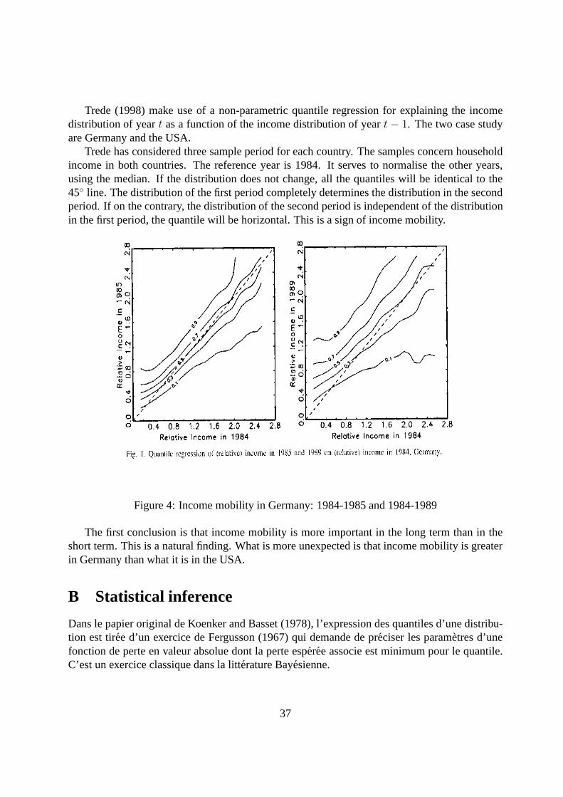
Trede (1998) make use of a non-parametric quantile regression for explaining the incomedistribution of yeart as a function of the income distribution of yeart − 1. The two case studyare Germany and the USA.

Trede has considered three sample period for each country. The samples concern householdincome in both countries. The reference year is 1984. It serves to normalise the other years,using the median. If the distribution does not change, all the quantiles will be identical to the45◦ line. The distribution of the first period completely determines the distribution in the secondperiod. If on the contrary, the distribution of the second period is independent of the distributionin the first period, the quantile will be horizontal. This is asign of income mobility.

Figure 4: Income mobility in Germany: 1984-1985 and 1984-1989

The first conclusion is that income mobility is more important in the long term than in theshort term. This is a natural finding. What is more unexpectedis that income mobility is greaterin Germany than what it is in the USA.

B Statistical inference

Dans le papier original de Koenker and Basset (1978), l’expression des quantiles d’une distribu-tion est tiree d’un exercice de Fergusson (1967) qui demande de preciser les parametres d’unefonction de perte en valeur absolue dont la perte esperee associe est minimum pour le quantile.C’est un exercice classique dans la litterature Bayesienne.

37

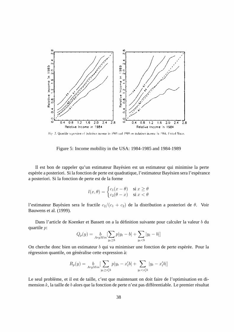
Figure 5: Income mobility in the USA: 1984-1985 and 1984-1989

Il est bon de rappeler qu’un estimateur Bayesien est un estimateur qui minimise la perteesperee a posteriori. Si la fonction de perte est quadratique, l’estimateur Bayesien sera l’esperancea posteriori. Si la fonction de perte est de la forme

l(x, θ) =

{c1(x− θ) si x ≥ θc2(θ − x) si x < θ

l’estimateur Bayesien sera le fractilec2/(c1 + c2) de la distribution a posteriori deθ. VoirBauwens et al. (1999).

Dans l’article de Koenker et Bassett on a la definition suivante pour calculer la valeurb duquartilep:

Qp(y) = bArgMin

[∑

yt≥b

p|yt − b| +∑

yt<b

|yt − b|]

On cherche donc bien un estimateurb qui va minimiser une fonction de perte esperee. Pour laregression quantile, on generalise cette expression a:

Rp(y) = bArgMin

[∑

yt≥x′

tb

p|yt − x′tb|+

∑

yt<x′

tb

|yt − x′tb|]

Le seul probleme, et il est de taille, c’est que maintenant on doit faire de l’optimisation en di-mensionk, la taille deb alors que la fonction de perte n’est pas differentiable. Lepremier resultat

38

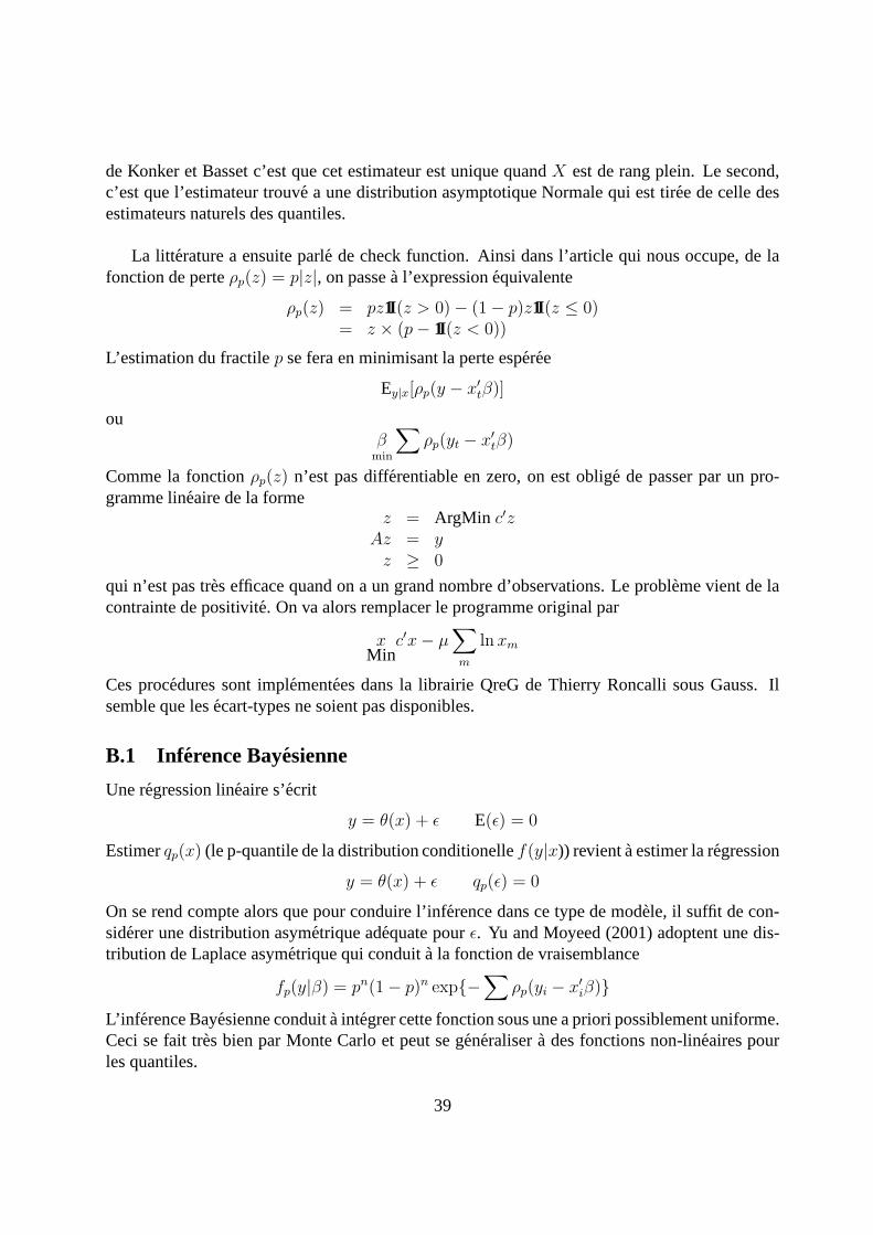
de Konker et Basset c’est que cet estimateur est unique quandX est de rang plein. Le second,c’est que l’estimateur trouve a une distribution asymptotique Normale qui est tiree de celle desestimateurs naturels des quantiles.

La litterature a ensuite parle de check function. Ainsi dans l’article qui nous occupe, de lafonction de perteρp(z) = p|z|, on passe a l’expression equivalente

ρp(z) = pz1I(z > 0)− (1− p)z1I(z ≤ 0)= z × (p− 1I(z < 0))

L’estimation du fractilep se fera en minimisant la perte esperee

Ey|x[ρp(y − x′tβ)]

ouβmin

∑ρp(yt − x′

tβ)

Comme la fonctionρp(z) n’est pas differentiable en zero, on est oblige de passer par un pro-gramme lineaire de la forme

z = ArgMin c′zAz = yz ≥ 0

qui n’est pas tres efficace quand on a un grand nombre d’observations. Le probleme vient de lacontrainte de positivite. On va alors remplacer le programme original par

xMin

c′x− µ∑

m

ln xm

Ces procedures sont implementees dans la librairie QreGde Thierry Roncalli sous Gauss. Ilsemble que les ecart-types ne soient pas disponibles.

B.1 Inference Bayesienne

Une regression lineaire s’ecrit

y = θ(x) + ε E(ε) = 0

Estimerqp(x) (le p-quantile de la distribution conditionellef(y|x)) revient a estimer la regression

y = θ(x) + ε qp(ε) = 0

On se rend compte alors que pour conduire l’inference dans ce type de modele, il suffit de con-siderer une distribution asymetrique adequate pourε. Yu and Moyeed (2001) adoptent une dis-tribution de Laplace asymetrique qui conduit a la fonction de vraisemblance

fp(y|β) = pn(1− p)n exp{−∑

ρp(yi − x′iβ)}

L’inference Bayesienne conduit a integrer cette fonction sous une a priori possiblement uniforme.Ceci se fait tres bien par Monte Carlo et peut se generaliser a des fonctions non-lineaires pourles quantiles.

39

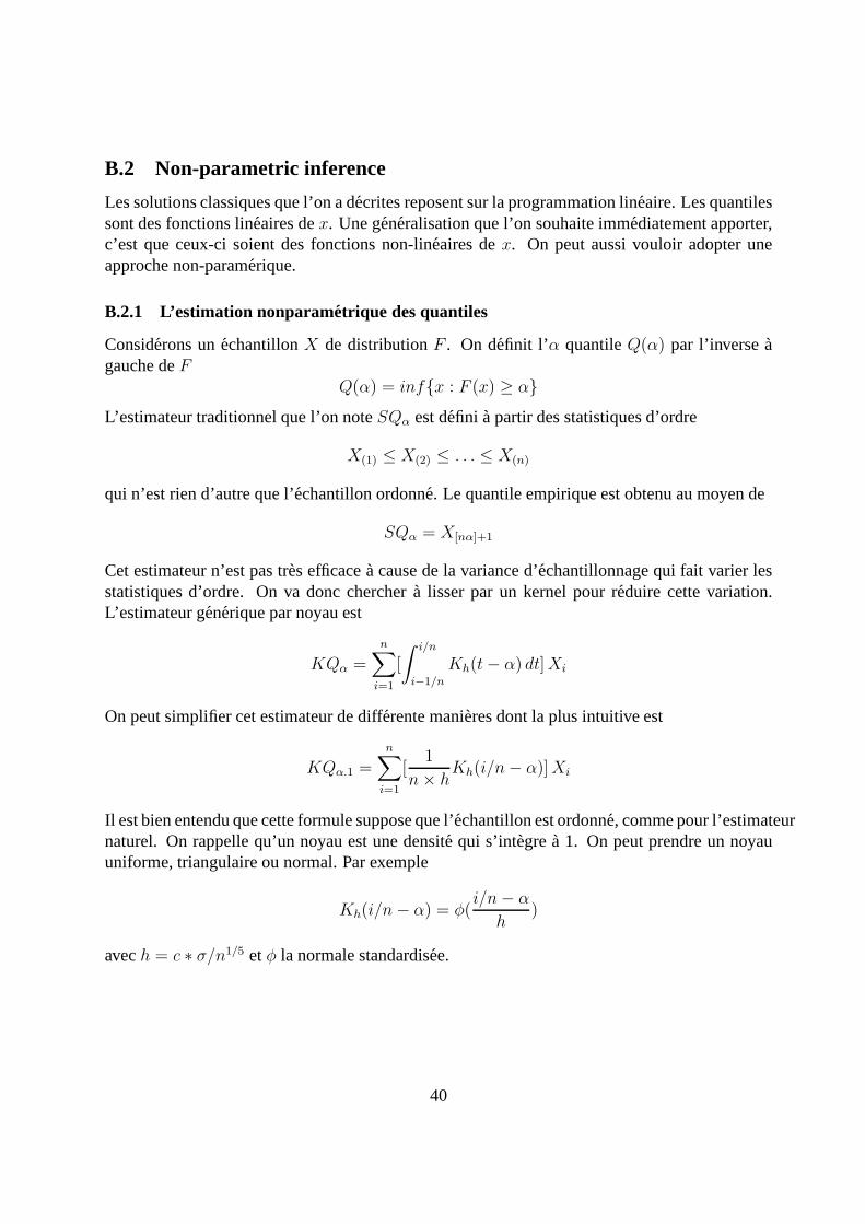
B.2 Non-parametric inference

Les solutions classiques que l’on a decrites reposent sur la programmation lineaire. Les quantilessont des fonctions lineaires dex. Une generalisation que l’on souhaite immediatement apporter,c’est que ceux-ci soient des fonctions non-lineaires dex. On peut aussi vouloir adopter uneapproche non-paramerique.

B.2.1 L’estimation nonparametrique des quantiles

Considerons un echantillonX de distributionF . On definit l’α quantileQ(α) par l’inverse agauche deF

Q(α) = inf{x : F (x) ≥ α}L’estimateur traditionnel que l’on noteSQα est defini a partir des statistiques d’ordre

X(1) ≤ X(2) ≤ . . . ≤ X(n)

qui n’est rien d’autre que l’echantillon ordonne. Le quantile empirique est obtenu au moyen de

SQα = X[nα]+1

Cet estimateur n’est pas tres efficace a cause de la variance d’echantillonnage qui fait varier lesstatistiques d’ordre. On va donc chercher a lisser par un kernel pour reduire cette variation.L’estimateur generique par noyau est

KQα =

n∑

i=1

[

∫ i/n

i−1/n

Kh(t− α) dt]Xi

On peut simplifier cet estimateur de differente manieres dont la plus intuitive est

KQα.1 =

n∑

i=1

[1

n× hKh(i/n− α)]Xi

Il est bien entendu que cette formule suppose que l’echantillon est ordonne, comme pour l’estimateurnaturel. On rappelle qu’un noyau est une densite qui s’int`egre a 1. On peut prendre un noyauuniforme, triangulaire ou normal. Par exemple

Kh(i/n− α) = φ(i/n− α

h)

avech = c ∗ σ/n1/5 etφ la normale standardisee.

40

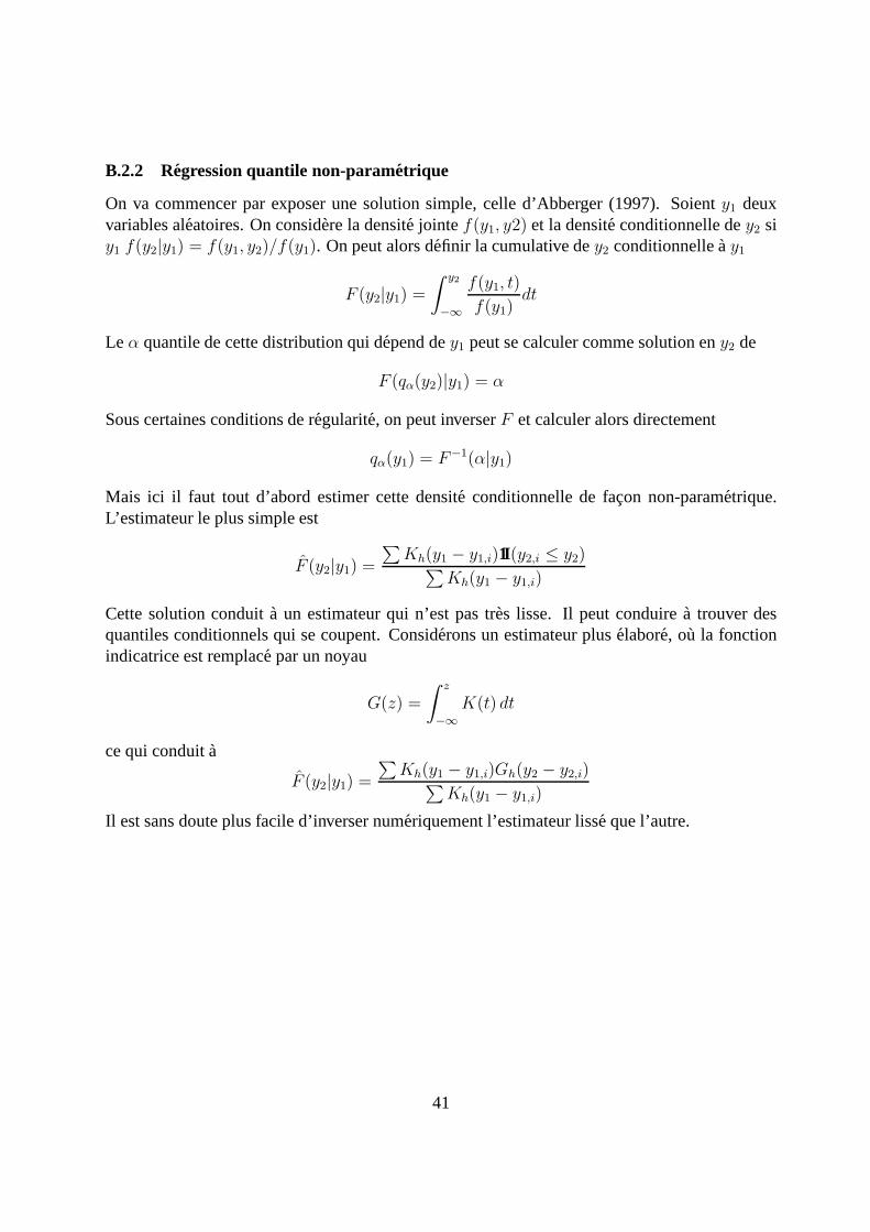
B.2.2 Regression quantile non-parametrique

On va commencer par exposer une solution simple, celle d’Abberger (1997). Soienty1 deuxvariables aleatoires. On considere la densite jointef(y1, y2) et la densite conditionnelle dey2 siy1 f(y2|y1) = f(y1, y2)/f(y1). On peut alors definir la cumulative dey2 conditionnelle ay1

F (y2|y1) =∫ y2

−∞

f(y1, t)

f(y1)dt

Le α quantile de cette distribution qui depend dey1 peut se calculer comme solution eny2 de

F (qα(y2)|y1) = α

Sous certaines conditions de regularite, on peut inverser F et calculer alors directement

qα(y1) = F−1(α|y1)

Mais ici il faut tout d’abord estimer cette densite conditionnelle de facon non-parametrique.L’estimateur le plus simple est

F (y2|y1) =∑

Kh(y1 − y1,i)1I(y2,i ≤ y2)∑Kh(y1 − y1,i)

Cette solution conduit a un estimateur qui n’est pas tres lisse. Il peut conduire a trouver desquantiles conditionnels qui se coupent. Considerons un estimateur plus elabore, ou la fonctionindicatrice est remplace par un noyau

G(z) =

∫ z

−∞

K(t) dt

ce qui conduit a

F (y2|y1) =∑

Kh(y1 − y1,i)Gh(y2 − y2,i)∑Kh(y1 − y1,i)

Il est sans doute plus facile d’inverser numeriquement l’estimateur lisse que l’autre.

41