the economic effects of density: a...
TRANSCRIPT

The economic effects of density: a synthesis
LSE Research Online URL for this paper: http://eprints.lse.ac.uk/100004/
Version: Published Version
Monograph:
Ahlfeldt, Gabriel M. and Pietrostefani, Elisabetta (2019) The economic effects of
density: a synthesis. International Trade and Regional Economics (DP13440).
Centre for Economic Policy Research, London School of Economics and Political
Science.
[email protected]://eprints.lse.ac.uk/
ReuseItems deposited in LSE Research Online are protected by copyright, with all rights reserved unless indicated otherwise. They may be downloaded and/or printed for private study, or other acts as permitted by national copyright laws. The publisher or other rights holders may allow further reproduction and re-use of the full text version. This is indicated by the licence information on the LSE Research Online record for the item.
DISCUSSION PAPER SERIES
DP13440
THE ECONOMIC EFFECTS OF DENSITY:A SYNTHESIS
Gabriel Ahlfeldt and Elisabetta Pietrostefani
INTERNATIONAL TRADE ANDREGIONAL ECONOMICS

ISSN 0265-8003
THE ECONOMIC EFFECTS OF DENSITY: ASYNTHESIS
Gabriel Ahlfeldt and Elisabetta Pietrostefani
Discussion Paper DP13440 Published 10 January 2019 Submitted 09 January 2019
Centre for Economic Policy Research 33 Great Sutton Street, London EC1V 0DX, UK
Tel: +44 (0)20 7183 8801 www.cepr.org
This Discussion Paper is issued under the auspices of the Centre’s research programme in INTERNATIONAL TRADE AND REGIONAL ECONOMICS. Any opinions expressed here arethose of the author(s) and not those of the Centre for Economic Policy Research. Researchdisseminated by CEPR may include views on policy, but the Centre itself takes no institutionalpolicy positions.
The Centre for Economic Policy Research was established in 1983 as an educational charity, topromote independent analysis and public discussion of open economies and the relations amongthem. It is pluralist and non-partisan, bringing economic research to bear on the analysis ofmedium- and long-run policy questions.
These Discussion Papers often represent preliminary or incomplete work, circulated toencourage discussion and comment. Citation and use of such a paper should take account of itsprovisional character.
Copyright: Gabriel Ahlfeldt and Elisabetta Pietrostefani

THE ECONOMIC EFFECTS OF DENSITY: ASYNTHESIS
Abstract
This paper synthesises the state of knowledge on the economic effects of density. We consider 15outcome categories and 347 estimates of density elasticities from 180 studies. More than 100 ofthese estimates have not been previously published and have been provided by authors onrequest or inferred from published results in auxiliary analyses. We contribute own estimates ofdensity elasticities of 16 distinct outcome variables that belong to categories where the evidencebase is thin, inconsistent or non-existent. Along with a critical discussion of the quality and thequantity of the evidence base we present a set of recommended elasticities. Applying them to ascenario that roughly corresponds to an average high-income city, we find that in per-capitapresent value terms (at a 5% discount rate), a 1%-increase in density implies an increase in wageand rent of $280 and $347. The decrease in real wage net of taxes of $156 is partiallycompensated for by an aggregate amenity effect of $100 and there is a positive external welfareeffect of $60.
JEL Classification: R38, R52, R58
Keywords: Compact, city, density, meta-analysis, Elasticity, present value
Gabriel Ahlfeldt - [email protected] and CEPR
Elisabetta Pietrostefani - [email protected]
AcknowledgementsThis work was financially supported by the OECD and the WRI. The results presented and views expressed here, however, areexclusively those of the authors. We acknowledge the help of 22 colleagues who contributed by suggesting relevant research,assisting with quantitative interpretations of their work, or providing additional estimates, including David Albouy, Victor Couture,Pierre-Philippe Combes, Paul Cheshire, Gilles Duranton, Patrick Gaule, Christian Hilber, Filip Matejka, Charles Palmer, and AbelSchumann. We also thank conference participants in Bochum (German regional economist meetings), Barcelona (IEB workshop),Copenhagen (UEA) and in particular David Albouy, Felipe Carozzi, Paul Cheshire, Jorge De la Roca, Pierre-Philippe Combes,Gerard Dericks, Steve Gibbons, Stephan Heblich, Christian Hilber, Walker Hanlon, Hans Koster, Andrei Potlogea, William Strange(the editor), Olmo Silva, Jens Südekum, Sevrin Waights, Jordy Meekes, and two anonymous referees for more general commentsand suggestions.
Powered by TCPDF (www.tcpdf.org)

Gabriel M. Ahlfeldt , Elisabetta Pietrostefani♠
The economic effects of density: A synthesis*
Abstract: This paper synthesises the state of knowledge on the economic effects of density. We consider 15
outcome categories and 347 estimates of density elasticities from 180 studies. More than 100 of these estimates
have not been previously published and have been provided by authors on request or inferred from published
results in auxiliary analyses. We contribute own estimates of density elasticities of 16 distinct outcome variables
that belong to categories where the evidence base is thin, inconsistent or non-existent. Along with a critical
discussion of the quality and the quantity of the evidence base we present a set of recommended elasticities.
Applying them to a scenario that roughly corresponds to an average high-income city, we find that in per-capita
present value terms (at a 5% discount rate), a 1%-increase in density implies an increase in wage and rent of
$280 and $347. The decrease in real wage net of taxes of $156 is partially compensated for by an aggregate
amenity effect of $100 and there is a positive external welfare effect of $60.
Key words: Compact, city, density, meta-analysis, elasticity, present value
Version: January 2019 JEL: R38, R52, R58
London School of Economics and Political Sciences (LSE) and Centre for Economic Policy Research
(CEPR), Houghton Street, London WC2A 2AE, [email protected], www.ahlfeldt.com ♠ London School of Economics and Political Sciences (LSE).
* This work was financially supported by the OECD and the WRI. The results presented and views
expressed here, however, are exclusively those of the authors. We acknowledge the help of 22 colleagues
who contributed by suggesting relevant research, assisting with quantitative interpretations of their
work, or providing additional estimates, including David Albouy, Victor Couture, Pierre-Philippe Combes,
Paul Cheshire, Gilles Duranton, Patrick Gaule, Christian Hilber, Filip Matejka, Charles Palmer, and Abel
Schumann. We also thank conference participants in Bochum (German regional economist meetings),
Barcelona (IEB workshop), Copenhagen (UEA) and in particular David Albouy, Felipe Carozzi, Paul
Cheshire, Jorge De la Roca, Pierre-Philippe Combes, Gerard Dericks, Steve Gibbons, Stephan Heblich,
Christian Hilber, Walker Hanlon, Hans Koster, Andrei Potlogea, William Strange (the editor), Olmo Silva,
Jens Südekum, Sevrin Waights, Jordy Meekes, and two anonymous referees for more general comments
and suggestions.

Ahlfeldt, Pietrostefani – The economic effects of density 2
1 Introduction
The degree of concentration of economic activity in urban areas is striking as they host more than 50% of the world’s population (United Nations 2014) on only an approximate 2.7% of the world’s land (GRUMP 2010; Liu et al. 2014).1 There is a consensus among planners and policymakers,
however, that even higher densities within cities and urban areas are desirable, at least on average
(Boyko & Cooper 2011; OECD 2012). Most countries pursue policies that implicitly or explicitly
aim at promoting “compact urban form”, reflecting the concern that unregulated economic markets will fail to deliver allocations of uses and infrastructures that are efficient and equitable
(IAU-IDF 2012; Holman et al. 2014). It is difficult to ascertain, however, to what extent this
normative statement prevailing in the policy debate can be substantiated by evidence (Neuman
2005).
To our knowledge, no attempt has been made to synthesise the evidence on the economic effects
of density and to compare the variety of costs and benefits across a comprehensive range of
outcome categories. It seems fair to state that the dominating “compact city” policy paradigm,
which aims at shaping the habitat of the urban population over the decades to come, is not
evidence-based. We make four contributions to address this notable gap in the literature.
Our first contribution is to provide a unique summary of the quantitative literature on the
economic effects of density. Our evidence base contains 347 estimates (from 180 studies) of the
effects of density on a wide range of outcomes including accessibility (job accessibility,
accessibility of private and public services), various economic outcomes (productivity, innovation,
value of space), various environmental outcomes (open space preservation and biodiversity,
pollution reduction, energy efficiency), efficiency of public service delivery, health, safety, social
equity, transport (ease of traffic flow, sustainable mode choice), and self-reported well-being.
While the evidence base is shared with a companion paper (Ahlfeldt & Pietrostefani 2017), the
results presented in the two papers are mutually exclusive. In the companion paper, we analyse
the effects of a variety of compact city characteristics (including morphological features and land
use mix), restricting the interpretation to qualitative results in order to explore the full evidence
base. In this paper, we focus on a quantitative comparison, and, therefore, restrict the analysis to
results that can be expressed as an elasticity of an outcome with respect to density. For more than
100 cases, we conduct back-of-the-envelope calculations to convert the results into a comparable
1 The estimates of the global urban land reported in the literature vary widely, from less than 0.3 to 3%
primarily because of the different definitions of urban land and data used (night light data, Landsat data
etc.) (Angel et al. 2005; GRUMP 2010; Liu et al. 2014). In 2010, the global urban land was close to 3%,
while the global built-up area was approximately 0.65%.
Ahlfeldt, Pietrostefani – The economic effects of density 3
metric or obtain results that had not previously been published from the relevant authors.
Borrowing techniques from meta-analytic research, we analyse within-category heterogeneity
with respect to characteristics such as the type of methods used, the citations adjusted for years
since publication, or the geographic setting of the analysis. In some instances, we make admittedly
ambitious assumptions to translate results published in fields such as engineering and medical
research into a format that is compatible with the conventions in economics and related
disciplines.
Our second contribution is to provide own elasticity estimates where the evidence base is thin or
inconsistent. We provide transparent density elasticity estimates based on a consistent
econometric framework and OECD data that refer to 16 distinct outcome variables (from 10
outcome categories). For some outcomes, such as the density elasticity of preserved green space,
our estimates are without precedent. We provide an estimate of the elasticity of density with
respect to city size, which facilitates a better comparison of the results from studies analysing the
effects of density and city size. To reconcile the evidence on the effects of density on wages, rents,
and various (dis)amenities, we also provide novel estimates of the density elasticity of
construction costs.
Our third contribution is to condense this broad evidence base into a set of 15 category-specific
density elasticities. Specific to each category, we either recommend the weighted (by adjusted
citations) mean across the elasticities in our evidence base, an estimate from a high-quality
original research paper or one of our own estimates. Along with the recommended elasticities, we
provide a critical discussion of the quality and the quantity of the evidence base, highlighting
priority areas for further research. The compact presentation of a variety of density elasticities in
a consistent format is unique in terms of accessibility and coverage and represents a convenient
source for research engaging with the quantitative interpretation of density effects.
Our fourth contribution is to monetise the economic effects of density. For each of the 15 outcome
categories, we compute the per capita present value (PV, at a 5% discount rate) of the effect of a
1% increase in density for a scenario that roughly corresponds to an average metropolitan area
in a developed country. For this purpose, we combine our recommended density elasticities with
several valuations of non-marketed goods such as time, crime and mortality risk, or pollution,
among many others. The monetary equivalents allow for a novel accounting of the costs and
benefits of density and how the net effect of density across a broad range of amenity and dis-
amenity categories aligns with estimates of quality of life based on cost-earning differentials.2
2 The indirect inference of quality of life from relative wages goes back to the work pioneered by Rosen
(1979) and Roback (1982) which has spurred a growing literature (see Albouy & Lue 2015 for a review).
Ahlfeldt, Pietrostefani – The economic effects of density 4
Our analysis reveals sizeable benefits and costs of density. A log-point increase in density is
associated with (log-point effects in parenthesis) higher wages (0.04), patent activity (0.21),
consumption variety value (0.12), preservation of green spaces (0.28), lower car use (0.05), as
well as lower average vehicle mileage (0.06), energy consumption (0.07), crime (0.085), and costs
of providing local public services (0.17). Density, however, is also associated with higher rents
(0.15), construction costs (0.55), pollution concentration (0.13), skill wage gaps (0.035), mortality
risk (0.09) as well as lower average speed (0.12) and self-reported well-being (0.004). Studies
that are more frequently cited, or use more rigorous methods, find less positive density effects (in
a normative sense), suggesting a role for the quality of evidence. Although more evidence would
be desirable to substantiate our findings, our analysis reveals some insights into geographic
heterogeneity in density elasticities. In non-high-income countries, the density elasticity of wages,
at 0.08, is twice as large in high-income countries. Mode choice is less responsive to density,
whereas the gains from density in terms of domestic energy consumption appear to be larger. In
the US, the density elasticity of skill wage gaps, at 0.057, is larger than in other developed
countries, and, unlike in the rest of the world, higher densities are associated with higher crime
rates. Our review of the literature also suggests that the effect of density on rents may not be log-
linear. The density elasticity of rent increases by 0.063 for every increase in population density
by 1000 inhabitants per square kilometre. We do not find a similar non-linearity in the density
elasticity of productivity, suggesting that convex costs lead to a bell-shaped net-agglomeration
benefits curve (Henderson 1974).
In our illustrative scenario, a 1% increase in density leads to an increase in the per capita present
value (infinite horizon, 5% discount rate) of wages and rents of $280 ($190 after taxes) and $347.
Summing up the monetary equivalents of all amenity and dis-amenity categories we find a clearly positive value, which is, however, not as large as the “compensating differential” (rent effect –
after-tax wage effect). While density seems to be a net amenity, our admittedly imperfect
accounting also suggests that part of the rent increase may be attributable to the higher cost of
providing space and is not exclusive to enjoyable amenities. Policy-induced densification may lead
to aggregate welfare gains. However, there may be a collateral net-cost to renters and first-time
buyers.3
Our analysis unifies important strands in the economics literature on the spatial organisation of
economic activity. We provide an explicit comparison of the magnitude of agglomeration benefits
on the production (e.g. Combes et al. 2012) and consumption side (e.g. Couture 2016), the effects
of urban form on innovation (e.g. Carlino et al. 2007), housing rent (e.g. Combes et al. 2018),
3 To be theoretically consistent this interpretation requires that residents are not fully mobile (e.g. because
they have location-specific preferences).
Ahlfeldt, Pietrostefani – The economic effects of density 5
quality of life (e.g. Albouy & Lue 2015), driving distances (Duranton & Turner 2018), road speeds
(Couture et al. 2018), public spending reduction (e.g. Hortas-Rico & Sole-Olle 2010), energy
consumption (Glaeser & Kahn 2010), skill-wage gaps (Baum-Snow & Pavan 2012) and self-
reported well-being (Glaeser et al. 2016), in addition to a range of density effects on outcomes
that have remained under-researched in the economics literature. Our findings also have
important policy implications as they suggest that densification policies are likely efficient but not
necessarily equitable.
Some words are due on the limitations of this ambitious synthesis. Most estimates summarised in
this review are associations in the data and not necessarily causal estimates. The causal
interpretation then rests on the assumption that the variation in density within and between cities
is largely historically determined by factors that have limited contemporaneous effects on
outcomes. Moreover, for individual-, firm-, and unit-based outcomes (e.g. wages, innovation, rent,
wellbeing), the collected density elasticities often capture composition effects. In general, the
quantitative results are best suited for an evaluation of the effects of densification policies applied
to individual cities (as opposed to all cities in a country) in the long run. Compared to wages and
mode choice, the evidence base for the other outcomes is generally underdeveloped. While for
some categories selected high-quality contributions are available, the nature of the evidence is at
best preliminary for others. Significant uncertainty surrounds any quantitative interpretation in
the categories urban green, income inequality, health, and well-being. We view these outcomes as
priority areas for further research into the effects of density. In general, the extant evidence base
consists of point estimates, so that heterogeneity in density effects across contexts and the density
distribution remains a key subject for future original research and reviews.
The remainder of this paper is organised as follows. In section 2, we provide an introduction into
the origins of density and some ancillary estimates that help with the interpretation of density
effects. In section 3, we lay out how the evidence base was collected and classified. Section 4
summarises the evidence by outcomes and attributes. Section 5 presents a discussion of our own
density elasticity estimates. Section 6 condenses the evidence (including our own estimates) to
15 outcome-specific density elasticities. Section 7 discusses the monetary equivalents of an
increase in density. The final section (8) concludes. We also provide an extensive technical
appendix with additional results and explanations, which is essential reading for those wishing to
use our quantitative results in further research (recommended elasticities and monetary
equivalents).

Ahlfeldt, Pietrostefani – The economic effects of density 6
2 Background
In this section, we provide some theoretical background and ancillary empirical analyses that will
guide the interpretation of the evidence base.
2.1 Origins of density
The first columns of Table 1 summarise the distribution of population density by OECD functional
urban areas (FUA), comparing the US to the rest of the world. While, on average, density in US
cities is relatively low, the variation, at a coefficient of variation of about one, is similarly striking
in both samples. Another notable insight from Table 1 is that the variation in density within US
FUAs is about two and a half times the variation across FUAs.
Tab. 1. Variation in density
(1) FUA, Non-US (2) FUA, US (3) FUA, US (4) Census tract, US
OECD data OECD data Census data Census data
Pop. Density Pop. density Pop. Density (PD) Tract PD - FUA mean
Level Ln Level Ln Level Ln Level Ln
Min 36 3.58 27 3.29 34 3.54 -1,947 -10.99
p1 55 4.01 27 3.29 34 3.54 -1,201 -3.18
p25 330 5.80 100 4.60 163 5.10 369 0.57
p50 580 6.36 179 5.19 371 5.92 1,295 1.44
p75 994 6.90 386 5.96 648 6.47 2,831 2.37
p99 4,652 8.44 1,661 7.42 1,947 7.57 31,388 4.28
Max 4,851 8.49 1,661 7.42 1,947 7.57 209,187 5.87
Mean 814 6.33 274 5.23 451 5.76 2,907 1.36
SD1 798 0.90 268 0.89 370 0.90 5,890 1.49
CV2 98.03% - 97.81% - 82.06% - 202.58% -
N 211 70 70 34,123
Notes: Population density in inhabitants per square kilometre. Functional urban area (FUA) data from OECD
(Columns 1 and 2). Census data matched to FUA shapefiles on GIS, aggregated to FUA (Columns 3 and 4) –
data includes only core FUA, excluding the commuting zones around them. City cores are defined using the
population grid from the global dataset Landscan (2000). 1 Standard Deviation. 2 Coefficient of variation.
Economic theory offers a range of explanations for this large variation in density. In a world
without internal or external scale economies, density naturally results from the fundamental
productivity and amenity value of a location. Exogenous geographic features such as fertile soil,
moderate climate, or access to navigable rivers attract economic activity, leading to growing cities.
Classic urban economics models predict that larger cities will be denser since positive within-city
transport costs limit horizontal urban expansion (Brueckner 1987). Urban growth, therefore,
drives up the average rent in a city, leading to lower use of space and a substitution effect on the
consumption side. Since building taller becomes profitable, higher rents lead to densification due
to a more intense use of land and a substitution effect on the supply side. Within cities, densities
are higher close to desirable locations (such as the CBD) where rents are particularly high to offset

Ahlfeldt, Pietrostefani – The economic effects of density 7
for transport cost. Transport innovations (e.g. mass-produced cars) allow for horizontal
expansion and, ceteris paribus, reduce urban density.
Reflecting the shift towards knowledge-based urban economies (Michaels et al. 2018), recent
models feature agglomeration externalities (Lucas & Rossi-Hansberg 2002; Ahlfeldt et al. 2015)
making density a cause and an effect of productivity and utility. This class of models features
multiple equilibria so that cities may be dense and monocentric or polycentric and dispersed. Yet,
due to agglomeration-induced path dependency, contemporary economic geography often
follows features that were important in the past, e.g. agricultural land suitability (Henderson et al.
2018) or portage sites (Bleakley & Lin 2012). Similarly, the compact monocentric city structure
that is characteristic for historic cities has been argued to be more resilient to shocks (e.g. natural
disasters, or transport innovations) in cities that were already large about a century ago, the time
when external returns and mass-produced presumably started to become increasingly important
(Ahlfeldt & Wendland 2013).
In practice, and at the heart of the policy dimension of this paper, density is also determined by
various land use regulations, such as urban growth boundaries, preservation policies, as well as
height, floor area ratio, and lot size regulations, which often have their origins in history (McMillen
& McDonald 2002; Siodla 2015). For a comprehensive review of the role of history in urban
economics research, see Hanlon & Heblich (2018).
Given the endogeneity of density, separating the effects of density on an economic outcome from
the effects of location fundamentals represents an identification challenge. Natural experiments
such as the division of a city due to exogenous political reasons (Ahlfeldt et al. 2015) are rare.
Plausible instruments for density are often difficult to find, although some researchers have
exploited geology as a factor that likely impacts on the distribution of economic activity, but not
on an economic outcome of interest (Combes et al. 2010). Our reading is that, for the most part,
the literature implicitly exploits the idea that much of the spatial variation in density is rooted in
history. Many of the results summarised below are informative to the extent that density is
determined by factors that were relevant in the past and have a limited direct effect on economic
outcomes today.
2.2 Density and city size
The relationship between city size and density is critical to the interpretation of our evidence base.
Given the theoretical link discussed above, it is perhaps not surprising that the literature refers to
actual density, the population normalised by the geographic size of a city, and city size, the total
population, interchangeably.

Ahlfeldt, Pietrostefani – The economic effects of density 8
Some researchers have attempted to disentangle the effects of density and city size (Cheshire &
Magrini 2009). At the heart of such a separation is the idea that different types of agglomeration
economies operate at different spatial resolutions (Andersson et al. 2016, 1093). Separating the
effects of city size and density corresponds to separating the effects of different agglomeration
economies (and diseconomies), some of which operate over large distances (such that city size
matters), while others are more localised (such that density matters). While separating the effects
of density and city size is interesting, it is also challenging because the geographic size of an
integrated urban area cannot grow infinitely, which implies that density and city size cannot vary
independently.
Our reading of the literature is that in most studies identifying density effects from between-city
(as opposed to within-city) comparisons, city population implicitly changes as city density
changes (and vice versa). The evidence from between-city comparisons reviewed here should be
interpreted in that light, since compact-city policies aiming at changing density while keeping
population constant may result in smaller effects, if there is a genuine city-size effect that is
independent from density. As an example, if productivity gains from labour market pooling
operated at the city scale over relatively large commuting distances without spatial decay,
increasing density while holding population constant would not increase productivity.
Reassuringly, the estimates from between-city and within-city studies (which hold population
constant) tend to be quite similar conditional on us making the following adjustment.
To translate estimated city size elasticities from the literature into density elasticities, we use an
estimate of the elasticity of (population) density with respect to city size (population) derived
from a multi-country FUA-level data set (OECD 2016) and the following empirical specification: ln(𝐴𝑖,𝑐) = 𝑎 ln(𝑃𝑖) + 𝜇𝑐 + 𝜀𝑖,𝑐 , (1)
where 𝐴𝑖,𝑐 is the geographic area of FUA i in country c, 𝑃𝑖 is the land area of the FUA, and 𝜇𝑐 is a
country fixed effect. The city size elasticity of density is implicitly determined as 𝑑 ln(𝑃𝑖/𝐴𝑖) /𝑑 ln(𝑃𝑖) = 𝛼 = 1 − 𝑎 . Compared to using the log of density as dependent variable, this estimation
strategy avoids the mechanical endogeneity problem that arises if population shows up on both
sides of the equation. Our preferred estimate of a is 0.57, which implies a city size elasticity of
density of 𝛼 = 0.43. Therefore, we expect density elasticities to be slightly more than twice as
large as population elasticities if the underlying economic mechanisms are the same. We note that
our estimate of a is broadly consistent with the 0.7 estimate for French cities by Combes et al
(2018). Details related to the estimation of equation (1), the estimation results, and the various
transformations used to standardise the results reported in the literature are reported in section
2 of the appendix.
Ahlfeldt, Pietrostefani – The economic effects of density 9
2.3 Density and the supply side
As discussed above, the positive city size elasticity of density results from an interplay of the
demand side and the supply side of the urban economy. Higher rents in larger cities lead to higher
densities. Higher densities, in turn, imply that it is more expensive to provide space, pushing rents
up. Larger cities are therefore theoretically expected to be denser and have higher rents, with the
latter being the cause and effect of higher construction costs. The empirical evidence is generally
in line with these expectations. Helsley and Strange (2008) provide anecdotal evidence of larger
cities having taller buildings. Gyourko and Saiz (2006) show that constructing a standard home is
more expensive in denser areas, even after controlling for differences in geography (high hills and
mountains), regulatory regimes (housing permits, regulatory chatter), and labour market
conditions (e.g. wages, unionisation). According to Ellis (2004), midrise stacked flats are twice as
expensive to construct as single-family detached housing. Ahlfeldt & McMillen (2018) estimate a
height elasticity of construction cost of 0.25 for small structures (five stories and below), and even
higher elasticities for taller structures. However, estimates of the effect of density on construction
cost that capture the changes in the composition of building types (a structure effect) as well as
changes in the cost of building equivalent units (a location effect) to our knowledge do not exist
to date.
To substantiate the interpretation of our evidence base, we therefore provide novel estimates of
the density elasticity of (per-unit) construction costs. We combine a micro-data set on building
constructions from Emporis with census tract level population and area data from the 2010 US
Census and the American Community Survey (ACS). In an alternative approach, we create a
construction cost index using structure-type-specific construction cost estimates from Ellis
(2004) and information on the structure-type composition from the ACS (Ruggles et al. 2017).
This index exclusively captures variation in construction costs due to the composition of structure
types (the structure effect). The density elasticity of this index can be combined with the density
elasticity of the cost of a standard home (the location effect) estimated by Gyourko and Saiz (2006)
to give the overall density effect.
From the results of both analyses, we conclude that 0.04–0.07 represent a conservative range for
the density elasticity of construction cost in the US. This estimate is a gross estimate that includes
all structure effects and location effects that are associated with density (including differences in
regulation, geology and labour market conditions that may be cause or effects of density). A
detailed discussion of the effects of density on construction cost is in appendix 2.2. We will return
to this parameter when reviewing the evidence on the effects of density on rents, wages and
amenities.
Ahlfeldt, Pietrostefani – The economic effects of density 10
3 The evidence base
3.1 Collection
In line with standard best-practice approaches of meta-analytic research, as reviewed by Stanley
(2001), our literature search is carried out in several stages.4 We do not impose any geographical
restrictions (with respect to the study area) and consider various geographic layers (from micro-
geographic scale to cross-region comparisons).
First, we conduct 260 separate searches for various combinations of category-specific keywords
(combinations of outcomes and empirically observed variables) in academic databases (EconLit,
Web of Science, and Google Scholar) and specialist research institute working paper series (NBER,
CEPR, CESIfo, and IZA). Second, we expand on relevant research strands by conducting an analysis
of citation trees. Third, we ask colleges in our research networks to recommend relevant research
(by personal mail and a call circulated in social media) and add studies that were previously
known to us or came up in discretionary searches. 5 We keep track of the stage at which the
evidence is added to control for a bias due to a potentially selective research network. To prevent
publication bias, we explicitly consider studies that were published as edited book chapters, PhD
theses, reports, in refereed journals or in academic working paper series (we were also open to
other types of publications). This process, which is described in more detail in the appendix to this
paper and in Ahlfeldt & Pietrostefani (2017), results in 268 relevant studies, which include 473
conceptually distinct analyses. We typically keep multiple estimates (analyses) from the same
study if they refer to different dependent variables or geographic areas.
A restriction to elasticity estimates that are explicitly reported in publications shrinks the sample
by about 50% to 242 analyses in 127 studies. We make some effort, however, to increase the
evidence base. We infer density elasticities from reported city size elasticities using the elasticity
of city size with respect to density discussed above. Similarly, we conduct back-of-the-envelope
calculations to approximate density elasticities if results are reported as marginal effects in levels,
semi-elasticities, or in graphical illustrations. We also make some adjustments to allow for a
consistent interpretation within categories. As an example, we convert the density elasticities of
land prices into density elasticities of housing rents assuming a Cobb-Douglas housing production
4 Recent examples of classic meta-analyses in economics include studies by Eckel and Füllbrunn (2015),
Melo et al. (2009), and Nitsch (2005).
5 At this stage, we were pointed to a literature on urban scaling in which city size is related to a variety of
outcomes. This literature is not part of this review, because unlike with the bulk of the evidence base, the
analysis is purely descriptive and not concerned with density (Bettencourt & Lobo 2016; Batty 2008;
Bettencourt 2013).

Ahlfeldt, Pietrostefani – The economic effects of density 11
function (Epple et al. 2010) and a land share of 0.25 (Combes et al. 2018; Ahlfeldt et al. 2015).
Finally, some authors kindly provided density elasticity estimates on request, which were not
reported in their papers (e.g. Couture 2016; Tang 2015; Albouy 2008). This way, we increase the
quantitative evidence base by more than 100 estimates to 347 analyses in 180 studies. The final
quantitative sample is comparable to the full sample (473 analyses from 268 studies) across a
range of characteristics that we introduce in the next subsections (see appendix section 2).
A more complete discussion of the various adjustments made to ensure comparability of the
evidence is in appendix section 2. A complete list of studies along with the encoded attributes
introduced in the following sections is provided in a separate appendix to this paper.
3.2 Attributes
We choose a quantitative approach to synthesise our broad and diverse evidence base. As with
most quantitative literature reviews we use statistical approaches to test whether existing
empirical findings vary systematically in the selected attributes of the studies, such as the
geographic context, the data or the methods used. Therefore, we encode the results and the
various attributes of the reviewed studies into variables that can be analysed using statistical
methods.
The typical approach in meta-analytic research is to analyse the findings in a very specific
literature strand. The results that are subjected to a meta-analysis are often parameters that have
been estimated in relatively similar econometric analyses. In such instances, it is useful to collect
specific information concerning the econometric setup. In contrast, the scope of our analysis is
much broader. Our aim is to synthesise the evidence on the economic effects of density across a
range of outcome categories. We consider studies from separate literature strands that naturally
use very different empirical approaches. The information we collect is, therefore, somewhat more
generic and includes the following attributes:

Ahlfeldt, Pietrostefani – The economic effects of density 12
i) The outcome category, one for the 15 categories (see Table A1 for details, appendix section 1)
ii) The dependent variable, e.g. wages, land value, crime rate iii) The study area, including the continent and the country iv) The publication venue, e.g. academic journal, working paper, book chapter, report v) The disciplinary background, e.g. economics, regional sciences, planning, etc. vi) The stage (1–3) at which an analysis is added to the evidence base (see Table A2) vii) The period of analysis viii) The spatial scale of the analysis, i.e. within-city vs. between-city ix) The methodological approach as defined by the Scientific Maryland Scale (SMS) used
by the What Works Centre for Local Economic Growth (2016) The variable can take the following values:
0. Exploratory analyses (e.g. charts). This score is not part of the original SMS 1. Unconditional correlations and OLS with limited controls 2. Cross-sectional analysis with comprehensive controls 3. Good use of spatiotemporal variation controlling for period and individual
effects, e.g. difference-in-differences or panel methods 4. Exploiting plausibly exogenous variation, e.g. by use of instrumental variables,
discontinuity designs or natural experiments 5. Reserved to randomised control trials (not in the evidence base)
x) The cumulated number of citations, adjusted for the years since publication, which we generate using yearly citations counts per study from Scopus. For non-journal publications, we impute the citation index using data from Google Scholar. Expectedly, our study-based index is closely correlated with journal quality as measured by the SNIP (Source Normalised Impact per Paper) score (Scopus 2016) and the SCImago Journal Rank (Scimago 2017). A detailed discussion is in appendix 1.2.
It is worth pointing out that, in the present context, a higher SMS score does not necessarily imply
a higher quality of the evidence. While exploiting plausibly exogenous variation (SMS 4) is
certainly desirable to separate the effects of density from unobserved location fundamentals, it is
less clear that having a greater set of covariates (SMS 2) improves the analysis if the controls are
potentially endogenous. One example frequently found in the literature that gives cause for
concerns is the inclusion of multiple variables that capture different shades of urban compactness
such as population density, building density and job centrality. Similarly, the inclusion of spatial
fixed effects (SMS 3) does not improve the identification if the fraction of the variation in density
that is most likely exogenous is cross-sectional, because it is determined by history (see discussion
in section 2.1). Given these ambiguities, our preferred measure for weighting the elasticities in the
evidence base is the citation index, which captures the impact an analysis has had within the
research community.
In Table 2 we tabulate the distribution of analyses included in this review by selected attributes
(as discussed above, one study can include several analyses). While our evidence base to some
extent covers most world regions, including the global south, there is a strong concentration of
studies from high-income countries and, in particular, from North America. The clear majority of
studies have been published in academic journals. The evidence base is diverse with respect to

Ahlfeldt, Pietrostefani – The economic effects of density 13
disciplinary background, with economics as the most frequent discipline, accounting for a share
of about 30%.
In Figure 1, we illustrate the distribution of publication years, the study period, and the type of
methods used, according to the SMS. The evidence, overall, is very recent, with the great majority
of studies having been published within the last 15 years, reflecting the growing academic interest
in the topic. Most studies use data from the 1980s onwards. A clear majority of studies score two
or more on the SMS, which means there is usually at least some attempt to disentangle density
effects from other effects, often including unobserved fixed effects and period effects.
Distinguishing between studies published before or after the median year of publication (2008)
reveals a progression towards more rigorous methods that score three or four on the SMS.
Tab. 2. Distribution of analyses by attributes I
World region Publication Discipline North America 208 Academic Journal 266 Economics 100
Europe 86 Working Paper 62 Transport 72
Asia 34 Report 14 Planning 48
South America 7 PhD 4 Urban Studies 42
World 4 Book chapter 1 Other 34
OECD 3 - - Regional Studies 24
non-OECD 3 - - Health 14
Oceania 1 - - Economic Geography 9
Africa 1 - - Energy 4
Notes: Assignment to disciplines based on publication venues. Studies contain multiple analyses if density effects
refer to multiple outcomes.
Fig. 1. Distribution of study period and quality of evidence
Notes: Kernel in the left panel is Gaussian. 2008 is the median year of publication. Scientific Methods Scale (SMS)
defined above (higher values indicate more rigorous methods).

Ahlfeldt, Pietrostefani – The economic effects of density 14
4 Density elasticities in the literature
4.1 Results by outcome category
In Table 3 we summarise the quantitative results in our evidence base. We made an effort to
condense the elasticity estimates into a limited number of outcome groups. Because of the great
variety of outcomes in the evidence base we frequently report more than one elasticity per
outcome category to which we will refer to in the remainder of the paper (indicated by ID).
Throughout this paper, all outcomes are expressed such that positive elasticities imply economic
effects that are typically considered to be positive in the relevant literatures.
Given the variety of outcomes we do not discuss each result here but leave it to the interested
reader to pick their finding of relevance. We note, however, that there is significant variation in
the quantity of the evidence base (N) and the quality of the underlying evidence (as well as other
attributes) and we urge these differences to be taken into account when considering the evidence.
Caution is warranted, not only when the evidence base is quantitatively small (small N), but also
when it is inconsistent. A useful indicator is a standard deviation (SD) that is large compared to
the mean, like, for example, pollution reduction. For a selected set of outcome groups (one per
category) we provide a critical discussion of the quantity and the quality of the evidence in section
4 of the appendix. We report the mean elasticity weighted by our citation index in Table 3. The
interested reader will find results using alternative weighting schemes in section 2 of the
appendix.

Ahlfeldt, Pietrostefani – The economic effects of density 15
Tab. 3. Outcome elasticities with respect to density
Elasticity of outcome Proportion Med. Mean Elasticityg
ID with respect to density N Poora Ac.b Econ.c With.d Yeare SMSf Mean S.D.
1 Labour productivity 47 0.19 0.79 0.74 0.06 2007 3.02 0.04 0.04
1 Total factor productivity 15 0.13 0.87 0.80 0.20 2004 2.80 0.06 0.03
2 Patents p.c. 7 0.00 1.00 0.14 0.00 2006 2.86 0.21 0.11
3 Rent 13 0.00 0.69 0.62 0.62 2013 3.00 0.15 0.13
4 Commuting reduction 36 0.03 0.56 0.08 0.56 2005 2.17 0.06 0.12
4 Non-work trip reduction 7 0.00 0.71 0.00 0.86 2005 2.00 -0.20 0.44
5 Metro rail density 3 0.00 1.00 0.00 1.00 2010 3.33 0.01 0.02
5 Quality of life 8 0.38 0.88 1.00 0.13 2014 3.00 0.03 0.07
5 Variety (consumption amenities) 1 0.00 1.00 0.00 0.00 2015 4.00 0.19 -
5 Variety price reduction 2 0.00 0.00 1.00 1.00 2016 4.00 0.12 0.06
6 Public spending reduction 20 0.00 1.00 0.05 0.00 2007 2.00 0.17 0.25
7 90th-10th pct. wage gap reduction 1 0.00 1.00 0.00 0.00 2004 4.00 0.17 -
7 Black-white wage gap reduction 1 0.00 0.00 1.00 0.00 2013 2.00 0.00 -
7 Diss. index reduction 3 0.00 1.00 0.33 0.00 2009 3.33 0.66 0.94
7 Gini coef. reduction 1 0.00 1.00 0.00 0.00 2010 4.00 4.56 -
7 High-low skill wage gap reduction 3 0.00 0.67 1.00 0.00 2013 4.00 -0.13 0.07
8 Crime rate reduction 13 0.00 0.69 0.15 0.92 2014 2.54 0.24 0.47
9 foliage projection cover 1 0.00 1.00 0.00 1.00 2015 1.00 -0.06 -
10 Noise reduction 1 0.00 1.00 0.00 0.00 2012 1.00 0.04 -
10 Pollution reduction 18 0.44 0.33 0.33 0.39 2014 2.83 0.04 0.47
11 Energy reduction: Domestic & driving 21 0.10 0.90 0.38 0.24 2010 1.81 0.07 0.10
11 Energy reduction: Public transit 1 0.00 1.00 1.00 0.00 2010 1.00 -0.37 -
12 Speed 2 0.00 0.00 1.00 0.00 2016 4.00 -0.12 0.01
13 Car usage (incl. shared) reduction 22 0.00 0.95 0.00 0.95 2004 2.00 0.05 0.07
13 Non-car use 76 0.05 0.79 0.00 0.86 2006 2.03 0.16 0.24
14 Cancer & other disease reduction 5 0.00 1.00 0.00 0.60 2000 2.40 -0.33 0.20
14 KSI & casualty reduction 4 0.00 1.00 0.00 0.00 2003 2.00 0.01 0.61
14 Mental-health 1 0.00 1.00 0.00 1.00 2015 2.00 0.01 -
14 Mortality reduction 3 0.00 1.00 0.00 0.00 2010 2.00 -0.36 0.17
15 Reported health 3 0.00 1.00 0.00 0.00 2013 1.00 -0.27 0.11
15 Reported safety 1 0.00 1.00 0.00 1.00 2015 2.00 0.07 -
15 Reported social interaction 6 0.00 0.17 0.83 0.00 2007 3.50 -0.13 0.19
15 Reported wellbeing 1 0.00 1.00 1.00 0.00 2016 3.00 0.00 -
Sum 347
Notes: a Poor countries include low-income and median-income countries according to the World Bank definition. b Published in academic journal. c Belongs to the economics discipline. d Exploits within-city variation. e Year of publication. f Scientific Methods Scale (SMS) defined in section 3.2 (higher values indicate more
robust methods). g Weighted by the citation index introduced in section 3.2 and appendix section 1.2.
Outcome categories correspond to ID as follows: 1: Productivity; 2: Innovation: 3: Value of space; 4: Job
accessibility; 5: Services access; 6: Efficiency of public services delivery; 7: Social equity; 8: Safety; 9: Open
space preservation and biodiversity; 10: Pollution reduction; 11: Energy efficiency; 12: Traffic flow: 13:
Sustainable mode choice; 14: Health; 15: Well-being.
4.2 Results by attributes
For a pooled analysis of the sources of heterogeneity in the evidence base, we normalise category-
specific elasticity estimates so that they have a zero mean and a unit standard deviation within
the outcome groups listed in Table 3. Figure 2 reveals that estimated density elasticities tend to
decline in the year of publication, the citation index, and the SMS score. This pattern is in line with
the increasing popularity of more rigorous methods displayed in Figure 1.
Ahlfeldt, Pietrostefani – The economic effects of density 16
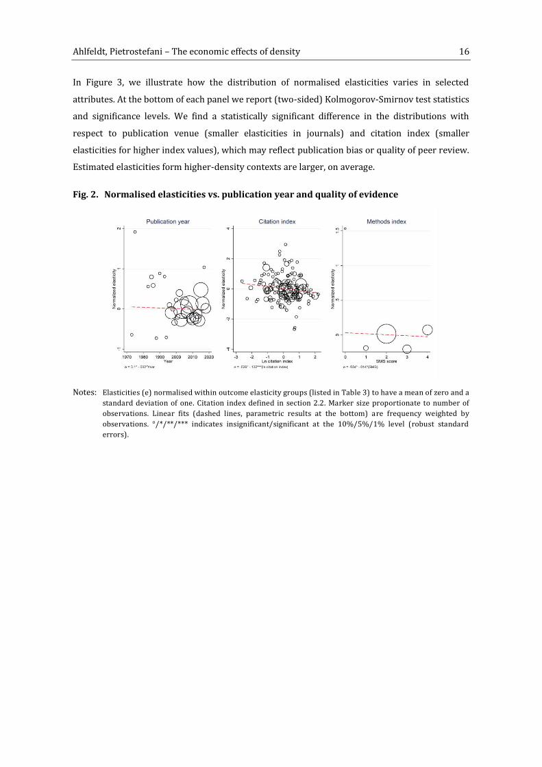
In Figure 3, we illustrate how the distribution of normalised elasticities varies in selected
attributes. At the bottom of each panel we report (two-sided) Kolmogorov-Smirnov test statistics
and significance levels. We find a statistically significant difference in the distributions with
respect to publication venue (smaller elasticities in journals) and citation index (smaller
elasticities for higher index values), which may reflect publication bias or quality of peer review.
Estimated elasticities form higher-density contexts are larger, on average.
Fig. 2. Normalised elasticities vs. publication year and quality of evidence
Notes: Elasticities (e) normalised within outcome elasticity groups (listed in Table 3) to have a mean of zero and a
standard deviation of one. Citation index defined in section 2.2. Marker size proportionate to number of
observations. Linear fits (dashed lines, parametric results at the bottom) are frequency weighted by
observations. °/*/**/*** indicates insignificant/significant at the 10%/5%/1% level (robust standard
errors).

Ahlfeldt, Pietrostefani – The economic effects of density 17
Fig. 3. Distribution of normalised elasticities by attributes
Notes: Elasticities normalised within outcome elasticity groups (listed in Table 3) to have a mean of zero and a
standard deviation of one. Non-high-income include low-income and median-income countries according to
the World Bank definition. The citation index (CI) defined in section 2.2. °/*/**/*** indicates
insignificant/significant at the 10%/5%/1% level based on a two-sample Kolmogorov-Smirnov test for
equality of distribution functions.
Table 4 presents the results of a multivariate analysis simultaneously controlling for all attributes
considered in Figure 3. We first run a pooled regression using the normalised density elasticity as
an outcome. Being published in an academic journal decreases elasticity by a 0.4 standard
deviation. In addition, a one standard-deviation increase in the citation index results in a 0.09
standard deviation reduction in the elasticity. The conditional effect of a high SMS score is
insignificant, but the point estimate is negative. So, in line with Figures 2 and 3, the overall
impression is that higher quality is associated with less positive density elasticity estimates.
In the remaining columns of Table 4, we perform meta-analyses (Stanley & Jarrell 1989; Melo et
al. 2009) of the raw elasticities in some of the more populated outcome categories. The first
interesting finding is that once we control for study fixed effects, we find that the density elasticity
of wages in non-high-income countries is about twice as large as for high-income countries
(column 3). It is worth noting that this effect is identified from one multi-country study covering
Brazil, China, and India, in addition to the US (Chauvin et al. 2016), which is why we do not add
further controls to save degrees of freedom. However, the unconditional citation-weighted mean
in the evidence base is 0.08 for non-high-income countries (from 9 analyses), confirming the
100% premium over high-income countries (see Table A11b in the appendix for a tabulation of
mean elasticities by high-income and non-high-income countries).

Ahlfeldt, Pietrostefani – The economic effects of density 18
The important second insight is that if the population density in the studied area increases by
1000 inhabitants per square kilometre, the estimated density elasticity of rent increase by 0.063,
on average. This effect is qualitatively and quantitatively consistent with recent evidence from
French cities. Combes et al. (2018) show that the elasticity can vary from 0.205 for a small urban
area to 0.378 for an urban area of the size of Paris. Applying the 0.063-estimate from Table 4,
column (4), this corresponds to an increase in density by 2,750 inhabitants per square kilometre,
which in turn corresponds to going from cities like Grenoble or Lens (1000/km²) to a city like
Paris (3,700/km²) (Demographia 2018). In line with Glaeser & Gottlieb (2008), we do not find a
similar effect of density on the density elasticity of wages. So it appears that increasing cost of
density rather than decreasing productivity gains curb agglomeration benefits, leading to a bell-
shaped net-agglomeration benefits curve (Henderson 1974).
The third relevant finding is that the density elasticities of sustainable mode choice are
significantly lower for non-high-income countries. A potential explanation that is consistent with
the large density elasticity of wages in developing countries is an indirect income effect that works
in the opposite direction of the direct density effect. While a compact urban form ceteris paribus
may favour alternative modes, higher incomes in more urbanised areas increase the affordability
of car trips. Fourth, the mean density elasticity of energy consumption reduction is much larger
when identified from studies exploring within-city variation. In this context, it is worth noting that
the citation-weighted unconditional mean density elasticity of energy consumption reduction, at
0.16, is much larger for non-high-income countries than for high-income countries. Given the
small numbers (two estimates from non-high-income countries), it is difficult to separate the
within-city and non-high-income country effects. It may be that within cities, population density is
generally more strongly correlated with the share of multi-family houses, which tend to be more
energy efficient. This relationship might be particularly strong in developing countries where
often high densities imply formal housing as opposed to informal housing (Henderson et al. 2016).

Ahlfeldt, Pietrostefani – The economic effects of density 19
Tab. 4. Meta-analysis of density elasticities
(1) (2) (3) (4) (5) (6) (7)
Normalised
density
elasticity
Density
elasticity of
wages
Density
elasticity of
wages
Density
elasticity of
rent
Density
elasticity of
commuting
reduction
Density
elasticity of
energy use
reduction
Density
elasticity of
sustainable
mode
choice
Category ID All 1 1 3 4 11 13
Non-high-income
country
-0.111
(0.25)
0.025
(0.02)
0.050***
(0.00)
- -0.247
(0.21)
-0.195
(0.26)
-0.162***
(0.04)
Not published in
academic journal
0.401**
(0.19)
0.004
(0.02)
-0.021
(0.07)
0.150
(0.13)
0.364***
(0.10)
0.164
(0.16)
Non-economics
discipline
0.043
(0.18)
0.007
(0.02)
-0.081
(0.07)
0.041
(0.07)
0.003
(0.06)
-
Round 3 a 0.077
(0.18)
0.022*
(0.01)
-0.109+
(0.06)
0.003
(0.06)
0.101*
(0.05)
-0.178**
(0.07)
Within-city variation -0.136
(0.18)
-0.020+
(0.01)
-0.146
(0.10)
-0.071
(0.07)
0.187**
(0.07)
-0.085
(0.11)
Citation index
normalised by s.d.
-0.091*
(0.05)
-0.005+
(0.00)
0.307+
(0.18)
0.058
(0.05)
-0.010
(0.01)
0.030
(0.04)
SMS >=3 -0.203
(0.16)
-0.014
(0.01)
-0.040
(0.08)
-0.025
(0.05)
0.070
(0.07)
-0.007
(0.09)
Pop. density in study
area (1000/km²)
-0.008
(0.01)
-0.005
(0.00)
0.063**
(0.03)
0.011
(0.07)
0.017
(0.04)
-0.001
(0.00)
Constant 0.000
(0.05)
0.048***
(0.01)
0.048***
(0.00)
0.131***
(0.02)
0.051**
(0.02)
0.115***
(0.02)
0.183***
(0.04)
Study effects - - Yes - - - -
N 337 47 47 13 36 21 76
r2 0.043 0.126 0.846 0.805 0.306 0.763 0.131
Note: Normalised elasticities in (1) are normalised within outcome groups (those listed in Table 3) to have a zero
mean and a unity standard deviation. Citation index normalised by the global standard deviation. All
explanatory variables are normalised to have a zero mean within outcome groups. 10 observations drop out
in (1) due to normalisation within categories with singular observations. Non-high-income countries
include low-income and median-income countries according to the World Bank definition. Population
density in study area is from Demographia World Urban Areas (2018). a Round 3 consists of previously
known evidence and recommendations by colleagues. Standard errors (in parentheses) are clustered on
studies (one study can contain multiple analyses, the unit of observation). + p < 0.15, * p < 0.1, ** p < 0.05, ***
p < 0.01
5 Own density elasticity estimates
While the evidence base on the quantitative effects of density summarised above is rich and
reasonably consistent for outcomes like productivity or mode choice, it is thinner and less
consistent for many other outcomes. To enrich the evidence base in some of the less-developed
categories, we contribute some transparent elasticity estimates using data from the OECD
functional urban area and regional statistics database and the following regression model:
ln(𝑌𝑖,𝑐) = 𝛽 ln (𝑃𝑖𝐴𝑖) + 𝜏 ln (𝐺𝑖𝑃𝑖 ) + 𝜇𝑐 + 𝜖𝑖,𝑐 , (2)

Ahlfeldt, Pietrostefani – The economic effects of density 20
where 𝑌𝑖,𝑐 is an outcome in city i in country c, 𝑃𝑖 , 𝐴𝑖 , 𝜇𝑐 are population, geographic area, and
country fixed effects as in equation (1), and 𝐺𝑖 is GDP. The coefficient of interest is 𝛽, which gives
the density elasticity of an outcome controlling for GDP per capita and unobserved cross-country
heterogeneity. Where either population or area forms part of the dependent variable, we
instrument population density using the (ln) rank within the national population density
distribution as an instrument. Table 5 summarises the key results. Full estimation results, in each
case for a greater variety of model specifications, are in the appendix (section 3).
We find a negative association between well-being and density, which seems to be more
pronounced across countries than within. Still, the results support the singular comparable result
found in the literature (Glaeser et al. 2016). Our results further support the average findings in
the evidence base, in that innovation (number of patents) increases in density and crime rates,
energy use (carbon emissions), and average road speeds decrease in density.
Conflicting with the mean elasticities in the evidence base reported in Table 3, we find that
pollution concentrations are higher in denser cities. At the local level, the effect of concentrating
sources of pollution in space dominates the effect of reduced aggregate emissions (due to shorter
car trips and more energy-efficient housing). Our estimate has been confirmed by two recent
studies (Carozzi & Roth 2018; Borck & Schrauth 2018). Furthermore, our results consistently
suggest that income inequality increases in density. Our results are qualitatively and
quantitatively (see the results for US cities reported in section 3.3 in the appendix) consistent with
Baum-Snow et al. (2017). But there is some contrast to the reviewed literature that has found
mixed results, with many studies pointing to lower inequalities at higher levels of economic
density. To reconcile the evidence, we note that the evidence base contains several case studies
on a within-city scale, but our comparison is across economic areas. It seems plausible that the
mechanisms affecting equity dimensions are different on a within-city (segregation) and a
between-city (skill complementarity) scale, but further research is required to substantiate this
intuition. We note that the statistically insignificant effect of density on crime (conditional on
country fixed effects), masks heterogeneity across US and non-US cities. In line with (Glaeser and
Sacerdote 1999), we find that crime rates increase in density for US cities, whereas the opposite
is true for other OECD countries.
Our estimates of the relationship between green coverage and population density are without
precedent. The elasticity of green density with respect to population density qualitatively depends
on the spatial layer of analysis. At regional level (administrative boundaries) the spatial units
cover both urban and rural areas. The negative elasticity likely reflects that an increase in
population implies a larger share of urban, at the expense of non-urban land. Functional economic
areas are designed to cover exclusively urban areas. The positive elasticity likely reflects that

Ahlfeldt, Pietrostefani – The economic effects of density 21
within an urbanised area, increasing population density preserves space for urban parks and
suburban forests. Because we focus on the effects of urban form in this paper, the latter is our
preferred estimate. We note that the relatively large elasticity estimated conditional on country
fixed effects is driven by a suspiciously large elasticity across US cities (>1.4), whereas the within-
country elasticity for the rest of the world is in line with the baseline elasticity from the cross-
sectional model excluding fixed effects. Therefore, in this case we prefer the conservative non-
fixed effects model. The elasticity of per capita green area with respect to population is negative,
as expected. Our preferred elasticity estimate (-0.283) is of roughly the same magnitude as the
elasticity of green space value with respect to population density of 0.3 (Brander & Koetse 2011)
suggesting that congestion (number of users) and the value of green space increase at roughly the
same rate.
Tab. 5. Own elasticity estimates
Ln patents p.c.a Ln broadband p.c.b Ln income quintile ratiob Ln Gini coefficient b
Ln dens. 0.349*** 0.129* 0.034*** 0.01 0.024 0.035** -0.007 0.025***
FE - Yes - Yes - Yes - Yes
IV - Yes - Yes - - - -
Ln poverty rateb
Ln poverty rateb Ln homicides p.c.b
Ln green densityb
(administrative)
Ln urban green densitya
(functional economic)
Ln dens. -0.013 0.032 -0.166*** -0.048 -0.267*** -0.245*** 0.283** 0.761*
FE - Yes - Yes - Yes - Yes
IV - Yes - Yes - Yes - Yes
Ln speeda,d
Ln green p.c.c Ln pollution (PM2.5)b Ln CO2 p.c.b freeway arterial
Ln dens. -0.717*** -0.239 0.220*** 0.124*** -0.224*** -0.173*** -0.008 -0.063***
FE - Yes - Yes - Yes - -
IV - Yes - - - Yes - -
Ln mortality rateb Ln mortality rate:
transportb
Ln life expectancy
at birthb
Ln self-reported well-
beingb Ln dens. -0.046*** -0.017 -0.150*** -0.099*** 0.013*** 0.007* -0.023*** -0.007**
FE - Yes - Yes - Yes - Yes
IV - Yes - Yes - - - -
Notes: Density (dens.) is population density (population / area). All models control for ln GDP p.c. Fixed effects
(FE) are by country. IV is rank of a city in the population density distribution within a country.a Data from
OECD.Stat functional economic areas.b Data from OECD.Stat administrative boundaries (large regions).c
Data from OECD.Stat administrative boundaries (small regions, excluding GDP control due to unavailability
of data for the US) d Speed data from Lomax et al (2010). Poverty line is 60% of the national median income.
Speeds are measured during peak time. * p < 0.1, ** p < 0.05, *** p < 0.01, with standard errors clustered on
FE where applicable.
6 Recommended elasticities
In Table 6 we condense the quantitative evidence, including our own estimates, into
recommended density elasticities which we provide for each outcome category. Specific to each
category, we either recommend a citation-weighted mean across the elasticities in our evidence
base as reported in Table 3, an estimate from a high-quality original research paper or one of our
Ahlfeldt, Pietrostefani – The economic effects of density 22
own estimates. The selected dedicated analyses use comprehensive data and make sensible choices in the research design, i.e. they avoid excessive “overcontrolling” for endogenous variables and exploit plausibly exogenous variation. In general, we prefer the citation-weighted mean in the
evidence base as well as estimates from dedicated high-quality original research papers over our
own estimates. We also prefer estimates from dedicated high-quality papers over the weighted
means in the evidence base if the evidence base is thin or inconsistent, in particular if the
recommended elasticity is in line with our own analysis of OECD data.
Our aim is to provide a compact and accessible comparison of density effects across categories.
The baseline results are best understood as referring to high-income countries. Where possible,
we acknowledge cross-country differences in Table 6. Nevertheless, we wish to remind the reader
that we likely miss substantial context-specific heterogeneity. Moreover, the quality and quantity
of the evidence base is highly heterogeneous across categories. We strongly advise to consult
section 4 in the appendix, which provides a discussion of the origin of each of the recommended
elasticities against the quality and quantity of the evidence base, before applying any of the
elasticities reported in Table 6 in further research. In general, the elasticities are to be interpreted
as associations and not necessarily as causal effects. They may capture the effects of unobserved
fundamental factors and are best understood as describing area-based effects that include
selection effects. We stress that significant uncertainty surrounds the effects of density on income
inequality, urban green, health, and self-reported well-being.
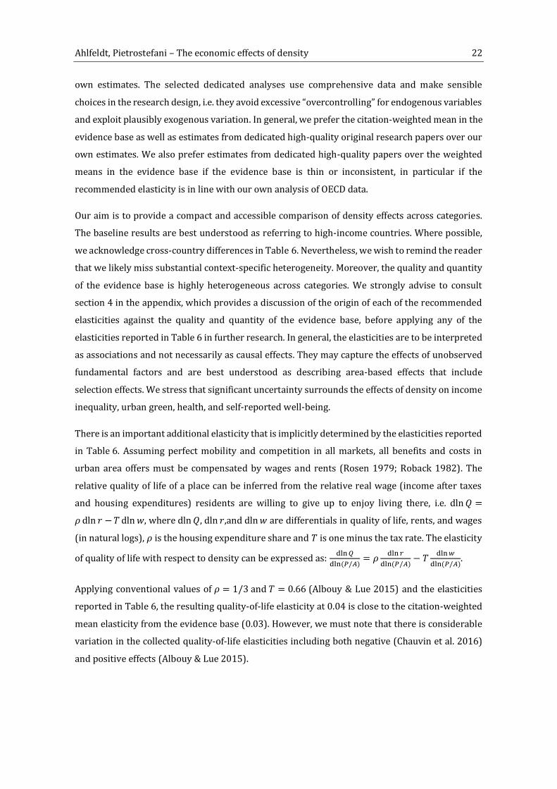
There is an important additional elasticity that is implicitly determined by the elasticities reported
in Table 6. Assuming perfect mobility and competition in all markets, all benefits and costs in
urban area offers must be compensated by wages and rents (Rosen 1979; Roback 1982). The
relative quality of life of a place can be inferred from the relative real wage (income after taxes
and housing expenditures) residents are willing to give up to enjoy living there, i.e. dln 𝑄 =𝜌 dln 𝑟 − 𝛵 dln 𝑤, where dln 𝑄, dln 𝑟,and dln 𝑤 are differentials in quality of life, rents, and wages
(in natural logs), 𝜌 is the housing expenditure share and 𝛵 is one minus the tax rate. The elasticity
of quality of life with respect to density can be expressed as: dln 𝑄dln(𝑃/𝐴) = 𝜌 dln 𝑟dln(𝑃/𝐴) − 𝛵 dln 𝑤dln(𝑃/𝐴).
Applying conventional values of 𝜌 = 1/3 and 𝛵 = 0.66 (Albouy & Lue 2015) and the elasticities
reported in Table 6, the resulting quality-of-life elasticity at 0.04 is close to the citation-weighted
mean elasticity from the evidence base (0.03). However, we must note that there is considerable
variation in the collected quality-of-life elasticities including both negative (Chauvin et al. 2016)
and positive effects (Albouy & Lue 2015).

Ahlfeldt, Pietrostefani – The economic effects of density 23
Tab. 6. Recommended elasticities by category
ID Elasticity Value Comment
1 Wage 0.04 Citation-weighted mean elasticity in review, roughly in line with
Melo et al. (2009). 0.08 for non-high-income countries. Net of
selection effects, the elasticity about halves Combes and Gobillon
(2015).
2 Patent intensity 0.21 Citation-weighed mean elasticity in review, in line with own
analysis of OECD data.
3 Rent 0.15 Citation-weighed mean elasticity in review. In line with evidence
from the US (dedicated analysis based on Albouy & Lue, 2015
data). Elasticity increases in density (own meta-analysis) and is
0.21 for France (Combes et al. 2018).
4 Vehicle miles travelled
(VMT) reduction
0.06 Citation-weighted mean elasticity in review, roughly in line with
Duranton & Turner (2018) and Ewing & Cervero (2010).
5 Variety value (price
index reduction)
0.12 Dedicated analysis on request using data from Couture (2016), in
line with Ahlfeldt et al. (2015).
6 Local public spending 0.17 Citation-weighted mean elasticity in review, roughly in line with
dedicated high-quality paper (Carruthers & Ulfarsson 2003).
7 Inter-quintile wage gap
reduction
-0.035 Own analysis of OECD dataa. -0.057 for the US. US estimate in line
with dedicated high-quality paper (Baum-Snow et al. 2017)
(section 3 in appendix).
8 Crime rate reduction 0.085 Dedicated analysis on request (Tang 2015), in line with own
analysis of OECD non-US city data. Dedicated high-quality paper
(Glaeser & Sacardote) and own analysis suggest a negative value
for the US.
9 Green density 0.28 Own analysis of OECD data (evidence base non-existent)
10 Pollution reduction -0.13 Dedicated high-quality paper (Carozzi & Roth 2018). In line with
Borck & Schrauth (2018) and own analysis of OECD data
11 Energy use reduction 0.07 Citation-weighted mean elasticity in review
12 Average speed -0.12 Citation-weighted mean of two (no further evidence) high-quality
papers (Duranton & Turner 2018; Couture et al. 2018)
13 Car use reduction 0.05 Citation-weighted mean elasticity in review
14 Mortality rate reduction -0.09 Dedicated paper (Reijneveld et al. 1999)
15 Self-reported well-being -0.0037 Only direct estimate in literature (Glaeser et al. 2016). In line with
own analysis of OECD data
Notes: Density elasticities are best understood as referring to large cities in high-income countries. In general, they
represent correlations and not necessarily causal estimates. If our recommended elasticities differ between
US and non-US cities, we report the former as the baseline and mention the latter in the comments, because,
as shown in Table 1, because the density distribution of US cities is not representative. a Own analysis uses
the wage gap between 80th and the. 20th percentile. 1: Productivity; 2: Innovation: 3: Value of space; 4: Job
accessibility; 5: Services access; 6: Efficiency of public services delivery; 7: Social equity; 8: Safety; 9: Open
space preservation and biodiversity; 10: Pollution reduction; 11: Energy efficiency; 12: Traffic flow: 13:
Sustainable mode choice; 14: Health; 15: Well-being. See appendix section 4 for a critical discussion of the
evidence base by category.
7 Monetary equivalents
For a quantitative comparison of density effects across categories, we conduct a series of back-of-
the-envelope calculations to express the effects that would result from a 1% increase in density
as per capita PV dollar effects, assuming an infinite horizon and a conventional 5% discount rate
(de Rus 2010). We summarise the results in Table 7. As most of the parameters used in the back-
of-the envelope calculations are context-dependent, the table is designed to allow for

Ahlfeldt, Pietrostefani – The economic effects of density 24
straightforward adjustments. The monetary effect in the last column (8) is simply the product
over the elasticity (3), the base value (5), the unit value (7), a 1% increase in density and the
inverse of the 5% discount rate (e.g. 0.04 × $35,000 × 1 × 1%/5% for the wage effect). By changing
any of the factors a context-specific monetary equivalent can be immediately calculated.
The exercise summarised in Table 7 is ambitious and there are some limitations. First, the
monetary equivalents most closely refer to large metropolitan areas in high-income countries. In
drawing conclusions for a specific institutional context, we strongly advise that the assumptions
made in appendix section 5 are evaluated with respect to their applicability. Second, the results in
Table 7 do not necessarily correspond to the short-run effect of a policy-induced change in
density. As an example, an increase in population holding the developed area constant will
increase population density, but not necessarily the green density. However, the green density
will be higher than in a counterfactual were the population growth was achieved holding density
constant. Third, the effects implied by the elasticities apply to marginal changes only, i.e. they
should not be used to evaluate the likely effects of extreme changes (e.g. a 100% increase in
density) in particular settings. Fourth, while for the not genuinely area-based outcomes we would
ideally apply density effects that come net of selection effects, the literature only offers such
estimates in the productivity category. So, for consistency across categories, we strictly apply the
baseline elasticities capturing area-based effects from Table 6. Section 5 in the appendix provides
a more detailed discussion of the evidence base that should be consulted before there is any
further use of the suggested monetary equivalents in Table 7.
Ahlfeldt, Pietrostefani – The economic effects of density 25
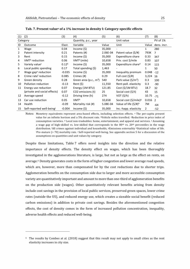
Tab. 7. Present valuea of a 1% increase in density I: Category-specific effects
(1) (2) (3) (4) (5) (6) (7) (8)
Category Quantity, p.c., year Unit value PV of 1%
ID Outcome Elast. Variable Value Unit Value dens. incr.
Incr.inc.inc. 1 Wage 0.04 Income ($) 35,000 - 1 280
2 Patent intensity 0.21 Patents (#) 2.06E-04 Patent value ($/#) 793K 7
3 Rent 0.15 Income ($) 35,000 Expenditure share 0.33 347
4 VMTb reduction 0.06 VMTb (mile) 10,658 Priv. cost $/mile 0.83 107
5 Variety valuec 0.12b Income ($) 35,000 Expenditure shared 0.14 115
6 Local public spending 0.17 Total spending ($) 1,463 - 1 50
7 Wage gape reduction -0.035 Income ($) 35,000 Inequality premium 0.048 -12
8 Crime ratef reduction 0.085 Crimes (#) 0.29 Full cost ($/#) 3,224 16
9 Green density 0.28 Green area (p.c., m²) 540 Park value ($/m²) 0.3 100
10 Pollution reduction -0.13 Rent ($) 11,550 Rent-poll. elasticity 0.3 -90
11 Energy use reduction
(private and social effects)
0.07 Energy (1M BTU) 121.85 Cost ($/1M BTU) 18.7 32 0.07 CO2 emissions (t) 25 Social cost ($/t) 43 15
12 Average speed -0.12 Driving time (h) 274 VOT ($/h) 10.75 -71
13 Car use reduction 0.05 VMTb 10,658 Social cost ($/mile)g 0.016 2
14 Health -0.09 Mortality risk (#) 5.08E-04 Value of life ($/#)h 7M -64
15 Self-reported well-beingj -0.004 Income ($) 35,000 Inc.-happ. elasticity 2 -52
Notes: Monetery equivalents represent area-based effects, including selection effects. a The per-capita present
value for an infinite horizon and a 5% discount rate. bVehicle miles travelled. cReduction in price index of
consumption varieties. d Local non-tradeables: home, entertainment, and apparel and services. e Assuming
a wage gap of high-skilled vs. low-skilled that corresponds to the 80th vs. 20th percentiles in the wage
distribution. fAll crimes against individual and households, gEmissions externality hStatistical value of life. iPre-mature (> 70) mortality rate. j Self-reported well-being. See appendix section 5 for a discussion of the
assumptions on quantities and unit values by category.
Despite these limitations, Table 7 offers novel insights into the direction and the relative
importance of density effects. The density effect on wages, which has been thoroughly
investigated in the agglomerations literature, is large, but not as large as the effect on rents, on
average.6 Density generates costs in the form of higher congestion and lower average road speeds,
which are, however, more than compensated for by the cost reductions due to shorter trips.
Agglomeration benefits on the consumption side due to larger and more accessible consumption
variety are quantitatively important and amount to more than one-third of agglomeration benefits
on the production side (wages). Other quantitatively relevant benefits arising from density
include cost savings in the provision of local public services, preserved green spaces, lower crime
rates (outside the US), and reduced energy use, which creates a sizeable social benefit (reduced
carbon emissions) in addition to private cost savings. Besides the aforementioned congestion
effects, the cost of density comes in the form of increased pollution concentration, inequality,
adverse health effects and reduced well-being.
6 The results by Combes at al. (2018) suggest that this result may not apply to small cities as the rent
elasticity increases in city size.
Ahlfeldt, Pietrostefani – The economic effects of density 26
Given that we have gone a long way in computing category-specific measures of costs and benefits
that are comparable across categories, a natural question arises: Do the benefits of density exceed
the costs and, if so, by how much? To address this question, we conduct a simple accounting
exercise in Table 8. We distinguish between private (columns 1–5) and external (column 6) costs
and benefits, which residents do not directly experience and likely do not pay for via rents (such
as reductions in carbon emissions that have global rather than local effects). To avoid double-
counting, we exclude gasoline costs in computing the benefits of shorter average trips (category
4) as this cost-saving is already accounted for by reduced energy consumption (category 11). Also,
we correct consumption benefits (category 5) to reflect the pure gains from variety and not
savings due to shorter car trips, which are already itemised in category (4). Since health effects
are itemised in 14, we use an estimate of the health cost arising from density-related pollution
from Carozzi & Roth (2018) to restrict the pollution effect to an amenity channel. The external
effect from sustainable mode choice (13) is already itemised in the external benefit of reduced
energy use (11) and is thus not counted separately. In the baseline scenario (Sum row), we assume
that public services are nationally funded. In an alternative accounting (indicated in the bottom of
the table), we assume that public services are locally funded, so that density-induced cost savings
fully capitalise into rents (via lower taxes).
The standard urban economics framework builds on the spatial equilibrium assumption, which
implies that individuals are fully mobile and competition in all markets is perfect. In this
framework, rents reflect the capitalised values of productivity and utility so that the sum over
rents and wages (column 1) amounting $627, p.c. can be interpreted as a welfare gain to which
the external welfare effects of $60 in column (6) can be added. The spatial equilibrium framework
is also the theoretical fundament for the economic quality-of-life literature mentioned above,
which infers place-specific amenity values from compensating differentials. With perfectly elastic
demand, an increase in rent that exceeds an increase in disposable income necessarily reflects a
positive quality-of-life effect.
If mobility is not perfect and/or there is heterogeneity in the preference for locations, rents will
not only reflect demand-side conditions (here, amenities), but also supply-side conditions,
because local demand is downward-sloping (Arnott & Stiglitz 1979). Increases in density – or the
policies that enforce increased density – may then also increase rents because the cost of
supplying space is higher. By implication, observed rent increases do not necessarily reflect
demand-driven capitalization effects exclusively, but potentially to some extent spatial
differences in the slope of the supply curve (Hilber & Vermeulen 2016; Hilber 2017).
Distinguishing these scenarios is notoriously difficult, but it is informative to compare the quality-
of-life effect inferred from wages and rents to the aggregate amenity effects across categories. If
Ahlfeldt, Pietrostefani – The economic effects of density 27
the accounting was precise and complete and demand was perfectly elastic, we would expect the
aggregate amenity effect to equal the quality-of-life effect.
The amenity effect reported in column (3) with an PV of $100 per capita, is substantial, but smaller
than the after-tax compensating differential ($156) in column (2), suggesting a role for the supply
side (as long as demand is locally downward-sloping). The role of self-reported well-being is
controversial as it is regarded either as a proxy for individual utility (Layard et al. 2008) or as a
component in the utility function that is traded against the consumption of goods and amenities
(Glaeser et al. 2016). Indeed, the amenity effect and the quality-of-life effect are closer if we
excluding the well-being effect as a (dis)amenity category. Similarly, the gap shrinks if we treat
local public services as fully locally financed, which implies that the savings are passed on to
individuals and are capitalised into rents.
To assess the potential relevance of density effects on rents that originate from the supply side,
we assume a share of structural value in housing of 75% (Ahlfeldt et al. 2015; Combes et al. 2018)
and compute a range for the monetary equivalent of the effect of a 1% density increase on
construction cost as 0.04–0.07 (density elasticity of construction cost, see section 2.3) x $35k
(income) x 75% (share of structure value) x 33% (expenditure share on housing) x 1% (change in
density) / 5% (discount rate) = $70–120. Thus, density-induced increases in the cost of housing
supply are a plausible alternative for the gap between amenity and quality-of-life effects of
demand is locally downward sloping. A complementary channel that strengthens the supply-side
argument is a scarcity land rent that results from policies that restrict the amount of usable land
to increase density (Gyourko et al. 2008; Mayer & Somerville 2000). A detailed discussion of the
effects of density on construction costs is in appendix section 2.2.
In columns (4) and (5) we change the perspective and ask how a policy-induced marginal increase
in the density of a city would affect residents. Because costs and benefits of density capitalise into
rents, the individual net-benefit depends on housing tenure. Given the positive amenity affect
from column (5), it is immediate that homeowners gain, on average, as they receive an amenity
benefit without having to pay a higher rent. If they were moving to another area, they would leave
the amenity gain behind, but would benefit from a higher housing value. Renters would be
negatively compensated for the amenity gain by higher rents, making the implications more
ambiguous (Ahlfeldt & Maennig 2015). The net benefit to homeowners is positive with a combined
amenity and wage effect of $291 or more (if there are tax savings or we abstract from the well-
being effect). There is a net cost to renters of up to $56 if we include well-being effects and assume
that there are no tax effects due to savings in public services. If we exclude the well-being effect
and allow for cost savings in public services to be passed on to renters via lower taxes, the net
benefit remains negative, but is close to zero. Of course, the flipside is that there is a positive

Ahlfeldt, Pietrostefani – The economic effects of density 28
external benefit to land owners and given the non-linearity in the density elasticity of rent
documented in Section 4.2 the effect on renters may be positive in supply-elastic markets.
Overall, the evidence suggests that density is a net amenity. This does not imply, however, that
everybody necessarily benefits from densification policies. Renters may be net losers of
densification because of rent effects that exceed amenity benefits. The negative net-effect is
consistent with a negative density effect on well-being if individuals are attached to some areas
more than others. If one is willing to believe that there are strong forces that prevent renters from
moving, a supply constraining effect of density can shift renters to a lower utility level, consistent
with a negative effect on well-being (or happiness). This is, however, an ambitious interpretation
of the evidence as it is impossible to claim full coverage and perfect measurement of amenity
effects. It is important to acknowledge that the difference between the amenity effect (in
column 3) and the quality-of-life effect (in column 2) of density could simply be due to
measurement error (e.g. missing items column 3). Research into the well-being effects of density
differentiated by tenure would be informative, but to our knowledge, has yet to be conducted.
Tab. 8. Present valuea effects of a 1% increase in density II: Accounting
(1) (2) (3) (4) (5) (6)
Outcome Factor Quality Amenity Effect on External
ID Category Incomes of life value Owner Renter welfare
1 Wage 280 -190b 0 190c 190c 0 2 Innovation 0 0 0 0 0 6
3 Value of space 347 347 0 0 -347 0
4 Job accessibility 0 0 87d 87d 87d 0
5 Services access 0 0 99e 99e 99e 0
6 Eff. of pub. services delivery 0 0 0 0 0 50
7 Social equity 0 0 0 0 0 -12
8 Safety 0 0 16 16 16 0
9 Urban green 0 0 100 100 100 0
10 Pollution reduction 0 0 -47f -47f -47f 0
11 Energy efficiency 0 0 32 32 32 15
12 Traffic flow 0 0 -71 -71 -71 0
13 Car use reduction 0 0 0 0 0 0g
14 Health 0 0 -64 -64 -64 0
15 Self-reported well-being 0 0 -52 -52 -52 0 Sum 627 152 100 291 -56 60 Excl. subj. well-being - - 152 342 -4 60
Locally financed pubic services - 106
340 -6 Factor incomes and externality 686 - - - - -
Locally financed pubic services 637 - - - - -
Notes: a The present value per capita for an infinite horizon and a 5% discount rate. All values in $. bAmenity
equivalent of after-tax wage increase assuming a marginal tax rate of 32% as in Albouy and Lue (2015). cAfter-tax wage increase as discussed in b. d Excludes $19.18 of driving energy cost ($0.15/mile gasoline
cost) discounted at 5%, which are itemised in 11 e Assumes a 10.2% elasticity to avoid double-counting of
road trips already included in 4. f Amenity effect, excludes health effect itemised in 14. g Set to zero to avoid
double counting with 11. Numbers reported in the “Locally financed pubic services” row assume that cost savings in local public services are fully passed on to residents via lower taxes.

Ahlfeldt, Pietrostefani – The economic effects of density 29
8 Conclusion
We provide the first quantitative evidence review of the effects of density on a broad range of
outcomes. Synthesising the reviewed evidence and a range of original estimates, we report
recommended density elasticities for 15 distinct outcome categories along with monetised values
of density effects for application in research and policy analysis. While there are sizeable benefits
and costs associated with increases in density, the former exceed the latter for a typical large city
in the developed world.
In general, much work lies ahead of the related research fields to consistently bring the evidence
base to the quantity and quality levels of the most developed outcome categories productivity and
mode choice. For all other categories, more research is required – even if selected high-quality
evidence exists – to substantiate the recommended elasticities. At this stage, significant
uncertainty surrounds any quantitative interpretation in the categories urban green, income
inequality, health, and well-being.
As research progresses and the quantity of the evidence base increases, evidence reviews and
meta-analyses become a more important aspect of knowledge generation. Regrettably, the scope
of this review was constrained because it was frequently not possible to translate results into a
comparable metric. To increase the scope of future reviews and meta-analyses, we encourage
researchers to complement the presentation of their preferred results by density elasticity
estimates that are comparable to those collected here. Minimally, complete summary statistics
need to be provided to allow for a conversion of reported marginal effects. Another feature that
hinders comparisons across studies is the common practice of analysing more than one aspect of
urban form at once, i.e. simultaneously using multiple spatial variables such as population density,
building density and job centrality. Disentangling the sources of the effects of compact urban form
is important. But it is difficult to compare such conditional marginal effects estimated under the
ceteris paribus condition across studies if the measures of urban form co-vary in reality because
they are simultaneously determined. To facilitate future reviews and meta-analyses we encourage
researchers to complement their differentiated analyses with simple models that exclusively
consider the most conventional measure of urban form, which is density.
We provide suggestive evidence that the costs and benefits of agglomeration may be larger in
developing-country cities. However, because the evidence from non-high-income countries is
scarce, it is not possible to property evaluate whether our key result that density is a net-amenity
generalises to non-high-income countries. An important challenge that lies ahead of the research
community is to generate a deeper understanding of heterogeneity in density effects across
contexts and the density distribution itself, a necessary condition for inference on optimal levels
of density.

Ahlfeldt, Pietrostefani – The economic effects of density 30
Literature
Ahlfeldt, G.M., Redding, S.J., Sturm, D.M. & Wolf, N., 2015. The Economics of Density: Evidence from the Berlin Wall. Econometrica, 83(6), pp.2127–2189.
Ahlfeldt, G.M. & Maennig, W., 2015. Homevoters vs. leasevoters: A spatial analysis of airport effects. Journal of Urban Economics, 87.
Ahlfeldt, G.M. & McMillen, D., 2018. Tall Buildings and Land Values: Height and Construction Cost Elasticities in Chicago, 1870–2010. The Review of Economics and Statistics, pp.861–875.
Ahlfeldt, G.M. & Pietrostefani, E., 2017. The compact city in empirical research: A quantitative literature review. SERC discussion paper 215. Ahlfeldt, G.M. & Wendland, N., 2013. How polycentric is a monocentric city ? Centers, spillovers and hysteresis. Journal of Economic Geography, 13(September 2012), pp.53–83.
Albouy, D., 2008. Are Big Cities Bad Places to Live? Estimating Quality of Life across Metropolitan Areas. National Bureau of Economic Research Working Paper 14472.
Albouy, D. & Lue, B., 2015. Driving to opportunity: Local rents, wages, commuting, and sub-metropolitan quality of life. Journal of Urban Economics, 89, pp.74–92.
Andersson, M., Klaesson, J. & Larsson, J.P., 2016. How Local are Spatial Density Externalities? Neighbourhood Effects in Agglomeration Economies. Regional Studies, 50(6), pp.1082–1095.
Angel, S., Sheppard, S.C., Civco, D.L., Buckley, R., Chabaeva, A., Gitlin, L., Kraley, A., Parent, J. & Perlin, M., 2005. The Dynamics of Global Urban Expansion, Washington D.C.
Arnott, R.J. & Stiglitz, J.E., 1979. Aggregate Land Rents, Expenditure on Public Goods, and Optimal City Size. The Quarterly Journal of Economics, 93(4), pp.471–500.
Batty, M., 2008. The size, scale, and shape of cities. Science, 319(5864), pp.769–71.
Baum-Snow, N., Freedman, M. & Pavan, R., 2017. Why Has Urban Inequality Increased ? Working
Paper.
Baum-Snow, N. & Pavan, R., 2012. Understanding the City Size Wage Gap. Review Econ Stud, 79(1), pp.247–253.
Bettencourt, L.M.A., 2013. The Origins of Scaling in Cities. Science, 340(6139), pp.1438–1441.
Bettencourt, L.M.A. & Lobo, J., 2016. Urban scaling in Europe. Journal of The Royal Society Interface, 13, pp.1–14.
Bleakley, H. & Lin, J., 2012. Portage and path dependence. Quarterly Journal of Economics, 127(2), pp.587–644.
Borck, R. & Schrauth, P., 2018. Population density and (urban) air quality. Preliminary and
Incomplete Working Paper.
Boyko, C.T. & Cooper, R., 2011. Clarifying and re-conceptualising density. Progress in Planning, 76(1), pp.1–61.
Brander, L.M. & Koetse, M.J., 2011. The value of urban open space: Meta-analyses of contingent valuation and hedonic pricing results. Journal of Environmental Management, 92, pp.2763–2773.
Brueckner, J.K., 1987. The structure of urban equilibria: A unified treatment of the muth-mills model. Handbook of Regional and Urban Economics, 2, pp.821–845.
Carlino, G.A., Chatterjee, S. & Hunt, R.M., 2007. Urban density and the rate of invention. Journal of
Urban Economics, 61(3), pp.389–419. Carozzi, F. & Roth, S., 2018. Dirty Density : Air Quality and the Denisty of American Cities. Preliminary and Incomplete Working Paper.
Carruthers, J.I. & Ulfarsson, G.F., 2003. Urban sprawl and the cost of public services. Environment

Ahlfeldt, Pietrostefani – The economic effects of density 31
and Planning B: Planning and Design, 30(4), pp.503–522.
Chauvin, J.P., Glaeser, E.L., Ma, Y. & Tobio, K., 2016. What is different about urbanization in rich and poor countries? Cities in Brazil, China, India and the United States. Journal of Urban
Economics, pp.1–33.
Cheshire, P. & Magrini, S., 2009. Urban growth drivers in a Europe of sticky people and implicit boundaries. Journal of Economic Geography, 9(1), pp.85–115.
Combes, G., Duranton, P.-P., Gobillon, L. & Roux, S., 2010. Estimating Agglomeration Economies with History, Geology, and Worker Effects. In E. L. Glaeser, ed. Agglomeration Economics. Chicago: Chicago University Press., pp. 15–66.
Combes, P.-P., Duranton, G., Gobillon, L., Puga, D. & Roux, S., 2012. The Productivity Advantages of Large Cities: Distinguishing Agglomeration From Firm Selection. Econometrica, 80(6), pp.2543–2594.
Combes, P.-P. & Gobillon, L., 2015. The Empirics of Agglomeration Economies. Handbook of
Regional and Urban Economics, 5, pp.247–348.
Combes, P., Duranton, G. & Gobillon, L., 2018. The Costs of Agglomeration: Land Prices in French Cities. The Review of Economic Studies, (7027).
Couture, V., 2016. Valuing the Consumption Benefits of Urban Density. Working Paper: Univeristy
of California, Berkeley, (September).
Couture, V., Duranton, G. & Turner, M.A., 2018. Speed. The Review of Economics and Statistics, 100(4), pp.735–739.
Demographia, 2018. Demographia World Urban Areas: 14th Annual Edition. Demographia, (April).
Duranton, G. & Turner, M.A., 2018. Urban form and driving: Evidence from US cities. Journal of
Urban Economics, 108, pp.170–191.
Eckel, C.C. & Füllbrunn, S.C., 2015. Thar SHE Blows? Gender, Competition, and Bubbles in Experimental Asset Markets. American Economic Review, 105(2), pp.906–920.
Ellis, J.G., 2004. Explaning Residential Density. Places, 16(2).
Epple, D., Gordon, B. & Sieg, H., 2010. American Economic Association A New Approach to Estimating the Production Function for Housing. American Economic Review, 100(3), pp.905–924.
Ewing, R. & Cervero, R., 2010. Travel and the Built Environment: A Synthesis. Journal of the
American Planning Association, 76(3), pp.265–294.
Glaeser, E.L. & Gottlieb, J.D., 2008. The Economics of Place-Making Policies. Brookings Papers on
Economic Activity, 2008(Spring), pp.155–253.
Glaeser, E.L., Gottlieb, J.D. & Ziv, O., 2016. Unhappy Cities. Journal of Labor Economics, 34(2), pp.S129–S182.
Glaeser, E.L. & Kahn, M.E., 2010. The greenness of cities: Carbon dioxide emissions and urban development. Journal of Urban Economics, 67(3), pp.404–418. Glaeser, E.L. & Sacerdote, B., 1999. Why is There More Crime in Cities ? Journal of Political
Economy, 107(No. S6 December 1999), pp.S225–S258.
GRUMP, 2010. Columbia University Socioeconomic Data and Applications Center Gridded Population of the World and the Global Rural-Urban Mapping Project. Available at: http://sedac.ciesin.columbia.edu/data/collection/gpw-v4 [Accessed January 7, 2017].
Gyourko, J. & Saiz, A., 2006. Construction costs and the supply of housing structure. Journal of
Regional Science, 46(4), pp.661–680.
Gyourko, J., Saiz, A. & Summers, A., 2008. A New Measure of the Local Regulatory Environment for Housing Markets: The Wharton Residential Land Use Regulatory Index. Urban Studies, 45(3),

Ahlfeldt, Pietrostefani – The economic effects of density 32
pp.693–729.
Hanlon, W. & Heblich, S., 2018. History and Urban Economics. Working Paper.
Helsley, R.W. & Strange, W.C., 2008. A game-theoretic analysis of skyscrapers. Journal of Urban
Economics, 64(1), pp.49–64.
Henderson, J.V., Venables, A.J., Regan, T. & Samsonov, I., 2016. Building functional cities. Science
(New York, N.Y.), 352(6288), pp.946–7.
Henderson, J.V., Squires, T., Storeygard, A. & Weil, D., 2018. The Global Distribution of Economic Activity: Nature, History, and the Role of Trade. The Quarterly Journal of Economics, pp.357–406.
Henderson, J.V., 1974. The sizes and types of cities. American Economic Review, 64(4), pp.640–656.
Hilber, C. & Vermeulen, W., 2016. The Impact of Supply Constraints on House Prices in England. The Economic Journal, 126(591), pp.358–405.
Hilber, C.A.L., 2017. The Economic Implications of House Price Capitalization: A Synthesis. Real
Estate Economics, 45(2), pp.301–339.
Holman, N., Mace, A., Paccoud, A. & Sundaresan, J., 2014. Coordinating density; working through conviction, suspicion and pragmatism. Progress in Planning, 101, pp.1–38.
Hortas-Rico, M. & Sole-Olle, A., 2010. Does Urban Sprawl Increase the Costs of Providing Local Public Services? Evidence from Spanish Municipalities. Urban Studies, 47(7), pp.1513–1540.
IAU-IDF, 2012. Document d’orientations stratégiques pour le fret en Ile-de-France à l’horizon 2025, Direction régionale et interdépartementale de l’Équipement et de l’Aménagement d’Île-de-France: Paris.
Layard, R., Mayraz, G. & Nickell, S., 2008. The marginal utility of income. Journal of Public
Economics, 92(8–9), pp.1846–1857. Liu, Z., He, C., Zhou, Y. & Wu, J., 2014. How much of the world’s land has been urbanized, really? A hierarchical framework for avoiding confusion. Landscape Ecology, 29(5), pp.763–771.
Lomax, T., Schrank, D., Turner, S., Geng, L., Li, Y. & Koncz, N., 2010. Real-Timing the 2010 Urban
Mobility Report,
Lucas, R.E. & Rossi-Hansberg, E., 2002. On the Internal Structure of Cities. Econometrica, 70(4), pp.1445–1476.
Mayer, C.J. & Somerville, C.T., 2000. Land use regulation and new construction. Regional Science
and Urban Economics, 30(6), pp.639–662.
McMillen, D.P. & McDonald, J.F., 2002. Land Values in a Newly Zoned City. Review of Economics and
Statistics, 84(1), pp.62–72.
Melo, P.C., Graham, D.J. & Noland, R.B., 2009. A meta-analysis of estimates of urban agglomeration economies. Regional Science and Urban Economics, 39(3), pp.332–342.
Michaels, G., Rauch, F. & Redding, S.J., 2018. Task Specialization in U.S. Cities From 1880 To 2000. Journal of the European Economic Assocation, forthcomin(August), pp.1–45.
Neuman, M., 2005. The Compact City Fallacy. Journal of Planning Education and Research, 25(1), pp.11–26.
Nitsch, V., 2005. Zipf zipped. Journal of Urban Economics, 57(1), pp.86–100.
OECD, 2012. Compact City Policies: A Comparative Assessment, OECD Green Growth Studies, OECD Publishing.
OECD, 2016. OECD Metropolitan area data.
Reijneveld, S.A., Verheij, R.A. & de Bakker, D.H., 1999. Relative importance of urbanicity, ethnicity and socioeconomic factors regarding area mortality differences. Journal of epidemiology and
community health, 53(7), pp.444–5.

Ahlfeldt, Pietrostefani – The economic effects of density 33
Roback, J., 1982. Wages, Rents, and the Quality of Life. Journal of Political Economy, 90, pp.1257–1278.
Rosen, S., 1979. Wages-based Indexes of Urban Quality of Life. In P. Mieszkowski & M. Straszheim, eds. Current Issues in Urban Economics. Baltimore: John Hopkins Univ. Press.
Ruggles, S., Genadek, K., Goeken, R., Grover, J. & Sobek, M., 2017. Integrated Public Use Microdata Series: Version 7.0 [dataset].
de Rus, G., 2010. Introduction to cost-benefit analysis : looking for reasonable shortcuts, Cheltenham, UK; Northampton, MA: Edward Elgar.
Scimago, 2017. SJR: Scientific Journal Rankings. Available at: http://www.scimagojr.com/journalrank.php [Accessed September 14, 2017].
Scopus, 2016. Journal Metrics. Available at: https://journalmetrics.scopus.com/ [Accessed September 14, 2017].
Siodla, J., 2015. Razing San Francisco: The 1906 disaster as a natural experiment in urban redevelopment. Journal of Urban Economics, 89, pp.48–61.
Stanley, T.D., 2001. Wheat From Chaff: Meta-Analysis As Quantitative Literature Review. Journal
of Economic Perspectives, 15(3), pp.131–150.
Stanley, T.D. & Jarrell, S.B., 1989. Meta-Regression Analysis: A Quantitative Method of Literature Surveys. Journal of Economic Surveys, 3(2), pp.161–170.
Tang, C.K., 2015. Urban Structure and Crime. Working Paper.
United Nations, 2014. World Urbanization Prospects: The 2014 Revision, New York.
What Works Centre for Local Economic Growth (WWC), 2016. Guide to scoring evidence using the
Maryland Scientific Methods Scale, London, UK.

Gabriel M. Ahlfeldt, Elisabetta Pietrostefani♠
Appendix to The economic effects of density: A synthesis Version: January 2019
Introduction
This appendix complements the main paper by providing additional detail not reported in the
main paper for brevity. To improve the flow of the presentation it partially duplicates discussions
in the main text. The appendix, however, is designed to complement, not replace the reading of
the main paper.
1 Evidence base
1.1 Collecting the evidence
In order to determine the selection of keywords to collect our evidence base we developed a
theory matrix through a transparent and theory-consistent literature search which can be found
in a companion paper (Ahlfeldt & Pietrostefani 2017). The theory matrix establishes the
economic channels connecting 15 outcome categories to three compact city characteristics. We
use combinations of keywords that relate to each outcome and compact city characteristic. Where
appropriate, we use empirically observed variables specified in the companion paper (Ahlfeldt &
Pietrostefani 2017).
London School of Economics and Political Sciences (LSE) and Centre for Economic Policy Research
(CEPR), Houghton Street, London WC2A 2AE, [email protected], www.ahlfeldt.com
♠ London School of Economics and Political Sciences (LSE).
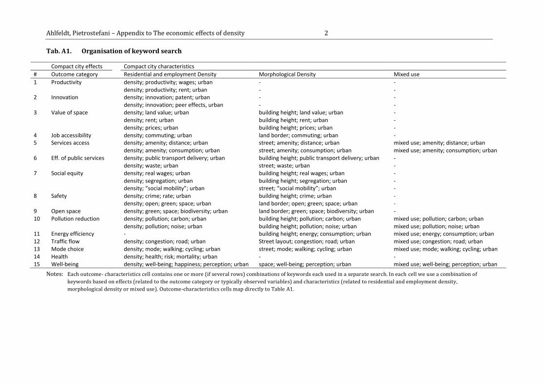
Ahlfeldt, Pietrostefani – Appendix to The economic effects of density 2
Tab. A1. Organisation of keyword search
Compact city effects Compact city characteristics
# Outcome category Residential and employment Density Morphological Density Mixed use
1 Productivity density; productivity; wages; urban - -
density; productivity; rent; urban - -
2 Innovation density; innovation; patent; urban - -
density; innovation; peer effects, urban - -
3 Value of space density; land value; urban building height; land value; urban -
density; rent; urban building height; rent; urban -
density; prices; urban building height; prices; urban -
4 Job accessibility density; commuting; urban land border; commuting; urban -
5 Services access density; amenity; distance; urban street; amenity; distance; urban mixed use; amenity; distance; urban
density; amenity; consumption; urban street; amenity; consumption; urban mixed use; amenity; consumption; urban
6 Eff. of public services density; public transport delivery; urban building height; public transport delivery; urban -
density; waste; urban street; waste; urban -
7 Social equity density; real wages; urban building height; real wages; urban -
density; segregation; urban building height; segregation; urban -
density; “social mobility”; urban street; “social mobility”; urban -
8 Safety density; crime; rate; urban building height; crime; urban -
density; open; green; space; urban land border; open; green; space; urban -
9 Open space density; green; space; biodiversity; urban land border; green; space; biodiversity; urban -
10 Pollution reduction density; pollution; carbon; urban building height; pollution; carbon; urban mixed use; pollution; carbon; urban
density; pollution; noise; urban building height; pollution; noise; urban mixed use; pollution; noise; urban
11 Energy efficiency - building height; energy; consumption; urban mixed use; energy; consumption; urban
12 Traffic flow density; congestion; road; urban Street layout; congestion; road; urban mixed use; congestion; road; urban
13 Mode choice density; mode; walking; cycling; urban street; mode; walking; cycling; urban mixed use; mode; walking; cycling; urban
14 Health density; health; risk; mortality; urban - -
15 Well-being density; well-being; happiness; perception; urban space; well-being; perception; urban mixed use; well-being; perception; urban
Notes: Each outcome- characteristics cell contains one or more (if several rows) combinations of keywords each used in a separate search. In each cell we use a combination of
keywords based on effects (related to the outcome category or typically observed variables) and characteristics (related to residential and employment density,
morphological density or mixed use). Outcome-characteristics cells map directly to Table A1.
Ahlfeldt, Pietrostefani – Appendix to The economic effects of density 3
We usually use the term density in reference to economic density and a more specific term to
capture the relevant aspect of morphological density. In several instances, we run more than one
search for an outcome-characteristics combination to cover different empirically observed
variables and, thus, maximise the evidence base. We note that because this way our search focuses directly on specific features that make cities “compact,” we exclude the phrase ‘compact city’ itself in all searches. Adding related keywords did not improve the search outcome in several trials, which is intuitive given that, by itself, “compactness” is not an empirically observable variable. In total, we consider the 52 keyword combinations (for 32 theoretically relevant
outcome-characteristic combinations) summarised in Table A1 which we apply to five databases,
resulting in a total of 260 keyword searches. We note that Google Scholar, unlike the other
databases, tends to return a vast number of documents, ordered by potential relevance. In several
trials preceding the actual evidence collection, we found that the probability of a paper being
relevant for our purposes was marginal after the 50th entry. Therefore, in an attempt to keep the
literature search efficient, we generally did not consider documents beyond this threshold.
In a limited number of cases we reassign a paper returned in a search for a specific outcome
category to another category if the fit is evidently better. Studies referring to economic density
may thus have sometimes been found through searches focused on other compact city
characteristics. Occasionally, a study contains evidence that is relevant to more than one category
in which case it is assigned to multiple categories. We generally refer to such distinct pieces of
evidence within our study as analyses. We do not double count any publication when reporting
the total number of studies throughout the paper and the appendix.
Based on the evidence collected in step one, we then conduct an analysis of citation trees in the
second step of our literature search. An important number of papers were added to the
productivity, innovation, job accessibility and mode choice categories through the citation tree
analysis (Tab A2). For papers that were not accessible through online resources, we reached out
to citing and cited authors. In a hand full of cases, we did not receive a response, the studies
therefore remain excluded. Upon inspection (excluding empirically irrelevant work, duplications
of working papers, and journal articles, etc.) this systematic literature search resulted in 195
studies and 313 analyses.
Up to this point, our evidence collection is unbiased in the sense that it mechanically follows from
the theory matrix (Ahlfeldt & Pietrostefani 2017) and is not driven by our possibly selective

Ahlfeldt, Pietrostefani – Appendix to The economic effects of density 4
knowledge of the literature, nor that of our research networks. For an admittedly imperfect
approximation of the coverage we achieve with this approach we exploit the fact that the search
for theoretical literature already revealed a number of empirically relevant studies that were not
used in the compilation of the theory matrix unless they contained significant theoretical thought.
From 19 empirically relevant papers known before the actual evidence collection, we find that
step one (keyword search) and two (analysis of citation trees) identified six, i.e., 31%.
In the final step 3 of the evidence collection we add all relevant empirical studies known to us
before the evidence collection as well as studies that were recommended to us by colleagues
working in related fields. To collect recommendations, we reached out by circulating a call via
social media (Twitter) and email (to researchers within and outside LSE). 22 colleagues
contributed by suggesting relevant literature. Further studies were suggested to us during
presentations of this paper and following our submission of this paper for publication. This step
increases the evidence base to 268 studies and 473 analyses (160 additional observations). The
evidence included at this stage may be selective due to particular views that prevail in our
research community. However, recording the stage at which a study is added to the evidence base
allows us to test for a potential selection effect.
Panel 1 of Table A2 summarises the collection process of the evidence base. We present the
number of studies found by category and the stage at which they were added to the evidence base.
Pane 2 of Table A2 summarises the distribution of analyses collected by outcome categories and
compact city characteristics. The large majority of 353 out of 473 analyses are concerned with
the effects of economic density, on which we focus in this paper. After restricting the sample to
analyses for which we are able to infer a density elasticity estimate, this number is reduced to
347. Table A3 compares the subsample of analyses for which we were able to compute an
outcome elasticity with respect to density to the universe of analyses, revealing only moderate
differences. The analyses in the elasticity subsample have a slightly higher propensity of being
added in the third evidence collection stage, a slightly higher mean SMS score (proxy for evidence
quality), and a somewhat higher propensity of showing positive (qualitatively) results.

Ahlfeldt, Pietrostefani – Appendix to The economic effects of density 5
Tab. A2. Evidence base by collection stage and research topic
Panel 1
# Outcome
Scholar
Web of
Science EconLit CesIfo
Step
2
Step
3 Total
1 Productivity 9 3 3 0 25 17 57
2 Innovation 3 1 2 1 5 1 13
3 Value of space 6 1 6 1 2 10 26
4 Job accessibility 3 1 3 0 19 5 31
5 Services access 2 0 1 0 0 8 11
6 Efficiency of public services delivery 2 0 1 0 0 4 7
7 Social equity 3 1 0 0 4 3 11
8 Safety 2 3 0 0 3 3 11
9
Open space preservation and
biodiversity 4 1 0 0 0 0 5
10 Pollution reduction 2 1 1 0 2 4 10
11 Energy efficiency 5 2 2 0 7 6 22
12 Traffic flow 2 0 0 0 1 1 4
13 Sustainable mode choice 7 3 1 0 27 5 43
14 Health 2 1 0 0 5 1 9
15 Well-being 2 0 1 0 0 5 8
Total 54 18 21 2 100 73 268
Panel 2
Compact city effects Compact city characteristics
# Outcome category Economic
density
Morph.
density
Mixed
land use
Total
1 Productivity 67 - - 67
2 Innovation 14 1 - 15
3 Value of space 18 8 2 28
4 Job accessibility 32 15 11 58
5 Services access 16 2 0 18
6 Efficiency of public services delivery 21 2 - 23
7 Social equity 13 0 - 13
8 Safety 19 4 - 23
9 Open space preservation and biodiversity 2 5 - 7
10 Pollution reduction 18 3 0 21
11 Energy efficiency 26 8 1 35
12 Traffic flow 4 2 1 7
13 Sustainable mode choice 76 33 17 126
14 Health 13 3 - 16
15 Well-being 14 2 0 16
Total 353 88 32 473
Notes: Panel 1: Google Scholar, Web of Science, EconLit, CesIfo searches all part of evidence collection step one.
Step 2 contains results from studies which were collected during step one but corresponded to a different
outcome to the one suggested by the keyword search they were found with, and studies from citation trees.
Step 3 consists of previously known evidence and recommendations by colleagues. Evidence base by
outcome category and compact city characteristic.
Panel 2: All numbers indicate the number of analyses collected within an outcome-characteristics cell. “0” indicates missing evidence in theoretically relevant outcome characteristic cell. “ -“ indicates missing evidence in theoretically irrelevant relevant outcome characteristic cell.

Ahlfeldt, Pietrostefani – Appendix to The economic effects of density 6
Tab. A3. All analyses vs. elasticity sample
All analyses Elasticity sample
Mean S.D. Mean S.D.
Non-high-income country a 0.11 0.31 0.084 0.28
Academic journal 0.79 0.41 0.77 0.42
Economics 0.26 0.44 0.29 0.45
Within-city 0.47 0.5 0.47 0.5
Round 3 d 0.34 0.47 0.4 0.49
Year of publication 2007 8.4 2008 6.9
Citation index 1.7 1.7 1.7 1.4
SMS (methods score) 2.2 1 2.4 0.86
Positive & significant b 0.67 0.47 0.69 0.46
Insignificant b 0.14 0.34 0.15 0.36
Negative & significant b 0.19 0.4 0.16 0.37
Qualitative result score c 0.48 0.8 0.53 0.76
N 473 347
Notes: Elasticity sample the sample of analyses from which a density elasticity could be inferred. a Non-high-
income include low-income and median-income countries according to the World Bank definition. b Qualitative results (positive, insignificant, negative) is a category-characteristics specific and defined in
Table A4. c Qualitative results scale takes the values of 1 / 0 / -1 for positive / insignificant / negative. d
Round 3 consists of previously known evidence and recommendations by colleagues.
1.2 Citation weights
For the SMS-based quality measure, we use a mapping of methods to quality ranks. Although we
closely follow an existing approach (What Works Centre for Local Economic Growth (WWC)
2016), the assignment of methods to quality scores involves individual judgement that is
potentially controversial. Moreover, the method used is at best an imperfect measure of the
quality of a research piece. Given these limitations, we develop, as an alternative, a citation-based
quality measure that is objective in the sense that it avoids individual judgements. With this
approach, we delegate the quality judgement to the wider research community, assuming that
better papers receive more attention. Still, to obtain a measure that is comparable across papers
we need to account for the obvious time trend in the probability of being cited. For this purpose, we recover a paper’s cumulated citation count adjusted for the years since publication as the fixed effect component 𝜇𝑝 from the following regression:
ln 𝐶𝑝𝑡 = 𝑓(𝑌𝑆𝑃𝑝) + 𝜇𝑝 + 𝜀𝑝𝑡
, where 𝐶𝑝𝑡 = ∑ 𝑐𝑝𝑡𝑧𝑧≤𝑡 , 𝑐𝑝𝑡𝑧 is the number of citations of a paper p in year t, 𝜀𝑝𝑡 is an idiosyncratic
component, and 𝑓(𝑌𝑆𝑃𝑝𝑡) is a function that describes how a paper’s cumulative citation count increases in the years a paper has been out.

Ahlfeldt, Pietrostefani – Appendix to The economic effects of density 7
To allow for non-linearities, given the lack of theoretical priors identifying the functional form,
we use a linear spline specification:
𝑓(𝑌𝑆𝑃𝑝𝑡) = 𝛼1𝑌𝑆𝑃𝑝𝑡 + ∑ 𝛼2(𝑌𝑆𝑃𝑝𝑡 − 𝑛) × (𝑌𝑆𝑃𝑝𝑡 − 𝑛 > 0)𝑛=2,5,10,20
, where (𝑌𝑆𝑃𝑝𝑡 − 𝑛 > 0) is a dummy variable that takes the value of one if the condition is true
and zero otherwise. In the figure below, we compare the fit provided by a linear spline function
allowing for changes in the marginal effect after 2, 5, 10, and 20 years since publications (dashed
lines) to a more flexible semi-non-parametric function (black circles). In this alternative
specification, we estimate a bin effect 𝛼𝑚 for every group of papers with the same number of
years since publication:
𝑓(𝑌𝑆𝑃𝑝𝑡) = ∑ 𝛼𝑚(𝑌𝑆𝑃𝑝𝑡 = 𝑚)𝑚>0
, where (𝑌𝑆𝑃𝑝𝑡 = 𝑚) is a dummy variable that is one if the condition is true, and zero otherwise.
Figure A1 suggests that the spline function overall provides a reasonable fit to the data generating
process. The bin effects are somewhat noisier for larger values of the year since publication
because only a fraction of papers in our data base have been out for such a long time, introducing
some selection effects. For this reason, we prefer the parametric spline function as a control for
year-since-publication effects.
We collect citation counts from Google Scholar and Scopus. The data was collected from the
summary tables of citation counts that both Google Scholar and Scopus provide starting from the
year of publication to today. Total number of citations for each source was also collected.
Figure A1 suggests that the rate at which citation counts increase in both data bases is roughly
comparable, although Google counts tend to be larger on average and increase a bit faster over
time for papers that have been out for a while.

Ahlfeldt, Pietrostefani – Appendix to The economic effects of density 8
Fig. A1. Cumulated citation counts vs. years since publication (within-paper effects)
Notes: Predicted values (excluding fixed effects) from regressions of the cumulated citation count of a paper against bin effects and a spline function controlling for paper fixed effects. Dot size proportionate to the number of papers in a bin.
In Figure A1, we compare the fixed effects components recovered from the Google Scholar and
the Scopus citation count regressions. The adjusted citation measures are highly correlated,
which is reassuring given neither data base provides full citations coverage. We select Scopus as
a baseline source because their counts are considered more reliable for a variety of reasons.
Scopus only indexes articles published in journals affiliated with its databases, but is the largest
abstract and citations database of peer-reviewed literature including research from science,
social sciences, humanities and other fields (Guide 2016). It not only includes citations counts for
journal articles but also trade publications, books and conference papers. Although Google
Scholar is increasingly used as a tool to collect citation impact, it has been shown to inflate
numbers of citations, be prone to double counting and does not have a clear indexing policy
(Moed et al. 2016; Harzing & Alakangas 2016). To achieve full coverage, we impute 26 missing
values in our Scopus-based adjusted citation measure using the Google-based adjusted citation
measure. In particular, we use predicted values from regressions of the Scopus measure against
the Google measure (corresponding to the dashed line in Figure A2).

Ahlfeldt, Pietrostefani – Appendix to The economic effects of density 9
Fig. A2. Google Scholar vs. Scopus adjusted citation indices
Notes: Solid line is the 45-degree line. Dashed line is the linear fit. Sample restricted to observations with positive Google Scholar and Scopus citation counts.
In Table A4, we correlate our adjusted citation index with the Source Normalised Impact per
Paper (SNIP) published by Scopus. This is a citation-based journal quality measure and it should
be positively correlated with our paper-based quality measure to the extent that our year-since-
publication adjustment results in a sensible approximation of the long-run impact of a paper.
Indeed, we find such a positive and statistically significant correlation. We also find that the there
is a significant trend in our (adjusted) citation count measure. Controlling for year-since-
publication effects, a paper published one year later attracts approximately 5% more citations.
The effects of the SNIP score and the publication year seem to be independent as the marginal
effects remain within close range across columns (1-3). The effects also remain within close range
if we control for differences in average number of citations across disciplines (4). Our adjusted
citation index is also positively correlated with the SCImago Journal Rank (5-6)

Ahlfeldt, Pietrostefani – Appendix to The economic effects of density 10
Tab. A4. Adjusted citations by paper vs. Scopus journal measures
(1) (2) (3) (4) (5) (6)
Ln Scopus
citation
adjusted
for years
since
publication
Ln Scopus
citation
adjusted
for years
since
publication
Ln Scopus
citation
adjusted
for years
since
publication
Ln Scopus
citation
adjusted
for years
since
publication
Ln Scopus
citation
adjusted
for years
since
publication
Ln Scopus
citation
adjusted
for years
since
publication
Ln SNIP score 0.798***
(0.17)
0.834***
(0.14)
1.001***
(0.14)
Year – 2000
0.051***
(0.01)
0.052***
(0.01)
0.054***
(0.01)
0.055***
(0.01)
Ln SJR score
0.360*** (0.08)
0.523*** (0.10)
Constant -0.332***
(0.12)
-0.186**
(0.09)
-0.654***
(0.12)
-0.759***
(0.07)
-0.063
(0.08)
-0.462***
(0.05)
Discipline effects - - - Yes - Yes
r2 0.112 0.203 0.325 0.398 0.072 0.371
N 225 225 225 225 225 225
Notes: Sample includes a subset of studies for which Scopus journal quality measures are available. Citation scores
adjusted for years since publications (in columns 1 and 3) are the study fixed effects recovered from
regressions of study-year Google citation counts against years since publication (a spline function) and
study fixed effects. A small number of observations is imputed using an auxiliary regression of the Google -
based citation measure against a similarly constructed Scopus-based measure. Citation scores adjusted for
year of publication and discipline are the residuals from a regression of the measures used in columns (1)
and (3) against discipline fixed effects and a yearly trend variable with a zero value in 2000. Disciplines are
defined based on outlets (journals and working paper series). SNIP is the Source Normalised Impact per
Paper and SJR is the SCImago Journal Rank, both published by Scopus. Scopus scores are averaged over
2011-2015. Robust standard errors in parentheses. * p < 0.1, ** p < 0.05, *** p < 0.01
In Table A5, we compare our adjusted citation index to the SMS methods score. A one step
increase on the SMS, on average, is associated with an increase in adjusted citations by some
notable 14% (1). The effect becomes insignificant once we control for discipline fixed effects, but
the point estimate increases (2). Once we control for the publication year trend, the positive
association disappears (3), suggesting that the positive correlation in (1) is driven by a common
time trend and that the two alternative quality measures are orthogonal to each other (in the
cross-section). Similarly, the journal-based SNIP is unrelated to the methods that prevail in the
published literature once we control for discipline effects (5-6).

Ahlfeldt, Pietrostefani – Appendix to The economic effects of density 11
Tab. A5. Citation measures vs. scientific methods scale
(1) (2) (3) (4) (5) (6)
Ln Scopus
citation
adjusted
for years
since
publication
Ln Scopus
citation
adjusted
for years
since
publication
Ln Scopus
citation
adjusted
for years
since
publication
Ln SNIP
score
Ln SNIP
score
Ln SNIP
score
Scientific methods
scale score
0.160**
(0.06)
0.234
(0.14)
0.074
(0.12)
0.074***
(0.03)
0.020
(0.04)
0.024
(0.04)
Year – 2000
0.048*** (0.01)
-0.001 (0.01)
Constant -0.292*
(0.17)
-0.456
(0.31)
-0.394
(0.24)
0.386***
(0.06)
0.507***
(0.09)
0.506***
(0.09)
Discipline effects - Yes Yes - Yes Yes
r2 0.027 0.081 0.234 0.031 0.181 0.182
N 258 258 258 228 228 228
Notes: Sample in columns (4-6) includes a subset of studies for which Scopus journal quality measures are
available. Citation scores adjusted for years since publications are the study fixed effects recovered from
regressions of study-year Google citation counts against years since publication (a spline function) and
study fixed effects. A small number of observations is imputed using an auxiliary regression of the Google-
based citation measure against a similarly constructed Scopus-based measure. Disciplines are defined
based on outlets (journals and working paper series). SNIP is the 2011-2015 average over the Source
Normalised Impact per Paper and SJR published by Scopus. Robust standard errors in parentheses. * p <
0.1, ** p < 0.05, *** p < 0.01
In Figure A3, we compare adjusted citation scores to the SMS scores by discipline. The values
plotted on the x-axis are the discipline fixed effects recovered from a regression of the Scopus
citation count adjusted for years since publication effects against discipline effects and a
publication year trend (the model from Table A5, column 3). The values on the y-axis are the
discipline fixed effects from similar regressions using our SMS scores as a dependent variable.
The figure suggests significant heterogeneity in the methods used as well as in the citation
probabilities across disciplines, but no significant correlation between the two.
It is possible that differences in the average citation counts across disciplines reflect a tendency
for researchers in some disciplines to cite relatively more frequently. This brings up the question
of whether such differences should be controlled for in a citation-based quality measure.
Controlling for discipline effects would impose the assumption that the average quality within
disciplines is the same across disciplines. This is a strong assumption; especially given that we
cover a potentially selective set of papers within each discipline. The high variation in the SMS
score across disciplines is certainly not suggestive of a constant average quality. We, therefore,
prefer not to control for cross-discipline differences in citation counts and, instead, assume that
such differences are driven by differences in the quality of the papers.
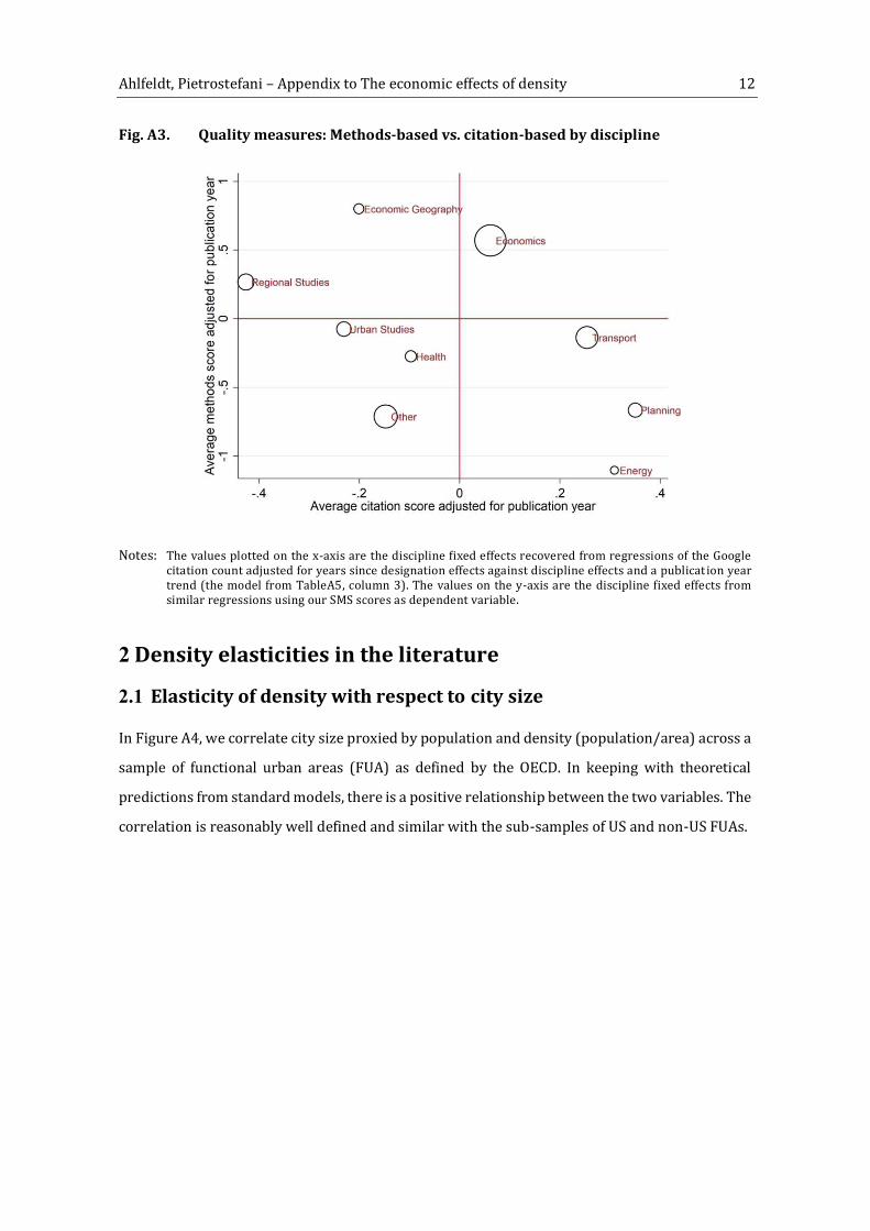
Ahlfeldt, Pietrostefani – Appendix to The economic effects of density 12
Fig. A3. Quality measures: Methods-based vs. citation-based by discipline
Notes: The values plotted on the x-axis are the discipline fixed effects recovered from regressions of the Google citation count adjusted for years since designation effects against discipline effects and a publicat ion year trend (the model from TableA5, column 3). The values on the y-axis are the discipline fixed effects from similar regressions using our SMS scores as dependent variable.
2 Density elasticities in the literature
2.1 Elasticity of density with respect to city size
In Figure A4, we correlate city size proxied by population and density (population/area) across a
sample of functional urban areas (FUA) as defined by the OECD. In keeping with theoretical
predictions from standard models, there is a positive relationship between the two variables. The
correlation is reasonably well defined and similar with the sub-samples of US and non-US FUAs.

Ahlfeldt, Pietrostefani – Appendix to The economic effects of density 13
Fig. A4. Population vs. population density
Notes: Dotted lines are the fitted lines from linear regressions. Non-US panel shows the partial correlation
controlling for country effects. Afunctional urban area (FUA) is labelled if the population is among the ten
largest or if it is an outlier. Outlies are below the 10th/5th or above the 90th/95th percentile in the US/Non-
US residual distribution. *** indicates significance at the 1% level.
We estimate the elasticity of density with respect to population using the following
straightforward econometric specification.
ln (𝑃𝑖𝐴𝑖) = 𝛼 ln(𝑃𝑖) + 𝜇𝑐 + 𝜀𝑖𝑐
, where 𝑃𝑖 is the population of city i, 𝐴𝑖 is the respective land area, and 𝜇𝑐 is a country fixed effect.
While the data theoretically allows us to estimate the elasticity from within-city variation over
time, we are concerned about the very limited within-city variation in land area in the data. An
imperfect measurement of changes in land area over time will lead to an upward bias in the
elasticity. In the extreme case, where land area does not change at all over time, the elasticity
would be mechanically one as the only variation on the left-hand side and the right-hand side
originates from population. To mitigate this problem, we prefer to estimate the elasticity from
cross-sectional between-city variation. Yet, there is still a potential mechanical endogeneity as
population (left-hand side) is also a component of density (right-hand side) so that any
measurement error in population will upward bias the elasticity. To address this problem, we
exploit that, mechanically, there is a negative relationship between the population of a city and
its rank in the population distribution within a city system. This negative relationship has been
analysed in a vast literature on city size distributions (Nitsch 2005). The rank of a city in the
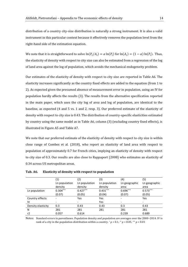
Ahlfeldt, Pietrostefani – Appendix to The economic effects of density 14
distribution of a country city-size distribution is naturally a strong instrument. It is also a valid
instrument in this particular context because it effectively removes the population level from the
right-hand side of the estimation equation.
We note that it is straightforward to solve ln(𝑃𝑖/𝐴𝑖) = 𝛼 ln(𝑃𝑖) for ln(𝐴𝑖) = (1 − 𝛼) ln(𝑃𝑖). Thus,
the elasticity of density with respect to city size can also be estimated from a regression of the log
of land area against the log of population, which avoids the mechanical endogeneity problem.
Our estimates of the elasticity of density with respect to city size are reported in Table A6. The
elasticity increases significantly as the country fixed effects are added to the equation (from 1 to
2). As expected given the presumed absence of measurement error in population, using an IV for
population hardly affects the results (3). The results from the alternative specification reported
in the main paper, which uses the city log of area and log of population, are identical to the
baseline, as expected (4 and 5 vs. 1 and 2, resp. 3). Our preferred estimate of the elasticity of
density with respect to city size is 0.43. The distribution of country-specific elasticities estimated
by country using the same model as in Table A6, column (3) (excluding country fixed effects), is
illustrated in Figure A5 and Table A7.
We note that our preferred estimate of the elasticity of density with respect to city size is within
close range of Combes et al. (2018), who report an elasticity of land area with respect to
population of approximately 0.7 for French cities, implying an elasticity of density with respect
to city size of 0.3. Our results are also close to Rappaport (2008) who estimates an elasticity of
0.34 across US metropolitan areas.
Tab. A6. Elasticity of density with respect to population
(1) (2) (3) (4) (5)
Ln population
density
Ln population
density
Ln population
density
Ln geographic
area
Ln geographic
area
Ln population 0.304***
(0.07)
0.427***
(0.05)
0.431***
(0.04)
0.696***
(0.07)
0.573***
(0.05)
Country effects - Yes Yes - Yes
IV - - Yes - -
Density elasticity 0.3 0.43 0.43 0.3 0.43
N 281 281 281 281 281
r2 0.057 0.614 0.239 0.689
Notes: Standard errors in parentheses. Population density and population are averages over the 2000–2014. IV is
rank of a city in the population distribution within a country. * p < 0.1, ** p < 0.05, *** p < 0.01
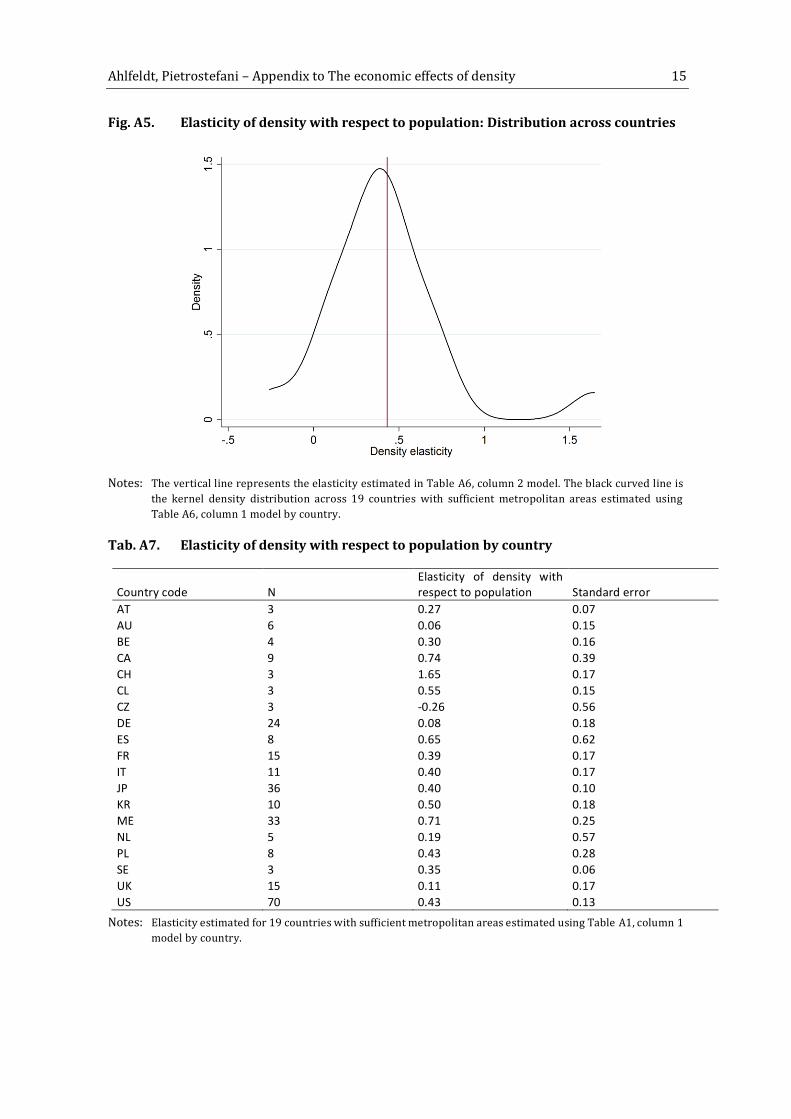
Ahlfeldt, Pietrostefani – Appendix to The economic effects of density 15
Fig. A5. Elasticity of density with respect to population: Distribution across countries
Notes: The vertical line represents the elasticity estimated in Table A6, column 2 model. The black curved line is
the kernel density distribution across 19 countries with sufficient metropolitan areas estimated using
Table A6, column 1 model by country.
Tab. A7. Elasticity of density with respect to population by country
Country code N
Elasticity of density with
respect to population Standard error
AT 3 0.27 0.07
AU 6 0.06 0.15
BE 4 0.30 0.16
CA 9 0.74 0.39
CH 3 1.65 0.17
CL 3 0.55 0.15
CZ 3 -0.26 0.56
DE 24 0.08 0.18
ES 8 0.65 0.62
FR 15 0.39 0.17
IT 11 0.40 0.17
JP 36 0.40 0.10
KR 10 0.50 0.18
ME 33 0.71 0.25
NL 5 0.19 0.57
PL 8 0.43 0.28
SE 3 0.35 0.06
UK 15 0.11 0.17
US 70 0.43 0.13
Notes: Elasticity estimated for 19 countries with sufficient metropolitan areas estimated using Table A1, column 1
model by country.

Ahlfeldt, Pietrostefani – Appendix to The economic effects of density 16
2.2 The elasticity of construction cost with respect to density
We assume that density impacts on construction costs through two principle channels. On the
one hand, constructing a dwelling unit with exactly the same specification is likely more
expensive in denser places because such places are usually more congested (higher cost of
moving materials, less space for construction), have higher construction worker wages, and are
more regulated (a location effect). On the other hand, while density can be achieved by reducing
housing consumption and increasing building density, it at least in the limit also requires taller
buildings, which are more expensive to construct (a structure effect). We are interested in the
gross effect of density on construction cost and, thus, in an estimate of the density elasticity of
construction cost that captures both location and the structure effects. To our knowledge, such
an estimate does not exist to date. However, Gyourko and Saiz (2006) provide estimates of the
density elasticity of construction cost using a construction cost index for a same-specification
home, which reflects on the effects of location exclusively. Ellis (2004), in contrast, provides a
construction cost index by dwelling type (various types of single-family and multifamily
structures) that holds all locational effects constant. In the remainder of this section we provide
two novel approaches to estimating the density elasticity of construction cost.
Frist, we make use of a micro-data set to compare how observed construction costs (excluding
costs for land acquisition) vary in density within and across cities. This approach directly yields
an estimate of the combined location and structure effect. Second, we create a construction cost
index that captures variation in the average construction cost across locations due to differences
in the structure composition, i.e. the structure effect. We then combine the estimated density
elasticity of this index with density elasticity estimates inferred from Gyourko and Saiz (2006),
which capture the locational effect, to obtain an estimate of the overall effect of density on
construction cost.
2.2.1 Estimates using micro-data
To our knowledge, no estimates of the effect of density on construction costs using actual
construction cost data exist to date. To fill this gap, we make use of a commercial data set
compiled by Emporis that has previously been used by Ahlfeldt & McMillen (2018). The data set
contains information on the date of construction, the height, and the number of floors for a large
number of buildings worldwide. Geo-information is provided in form of geographic coordinates
so that the location can be merged with other spatial data in GIS. The data set contains additional

Ahlfeldt, Pietrostefani – Appendix to The economic effects of density 17
building information, such as construction costs, use, or total floor space, however missing values
are present for a substantial fraction of constructions. While the data set is a unique source of
information on construction costs, its representativeness with respect to location and structure
type is not guaranteed. The intuition is that taller buildings at denser places will be
overrepresented in the data set as Emporis claims a nearly comprehensive coverage of tall
buildings such as skyscrapers. Against this background, it is reassuring to see that within the US-
sub-sample we use (containing information on construction cost and floor space, among other
characteristics), a large share of observations refers to small structures which account for the
majority of the building stock in US metropolitan areas (see also Figure A8). However, it is still
notable from Figure A6 that low-density census tracts are underrepresented in the data set we
analyse, suggesting that we obtain local elasticity estimates representative for above-average
density areas. Within tracts with at least one Emporis observation, constructions are also more
concentrated than population, as revealed by a more than twice as large Herfindahl index
(0.0205% vs. 0.0097%).
Fig. A6. Distribution of buildings in micro-data by number of floor
Notes: Data from Emporis. Sample restricted to observations in the US with information on location, construction
year, construction cost, building area, building height and the number of floors. Constructions exceeding
20 floors excluded in the graph to improve the presentation.
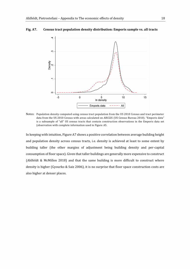
Ahlfeldt, Pietrostefani – Appendix to The economic effects of density 18
Fig. A7. Census tract population density distribution: Emporis sample vs. all tracts
Notes: Population density computed using census tract population from the US 2010 Census and tract perimeter
data from the US 2010 Census with areas calculated on ARCGIS (US Census Bureau 2010). “Emporis data” is a subsample of “all” US census tracts that conta in construction observations in the Emporis data set
(observation with complete information used in Figure A5.
In keeping with intuition, Figure A7 shows a positive correlation between average building height
and population density across census tracts, i.e. density is achieved at least to some extent by
building taller (the other margins of adjustment being building density and per-capital
consumption of floor space). Given that taller buildings are generally more expensive to construct
(Ahlfeldt & McMillen 2018) and that the same building is more difficult to construct where
density is higher (Gyourko & Saiz 2006), it is no surprise that floor space construction costs are
also higher at denser places.
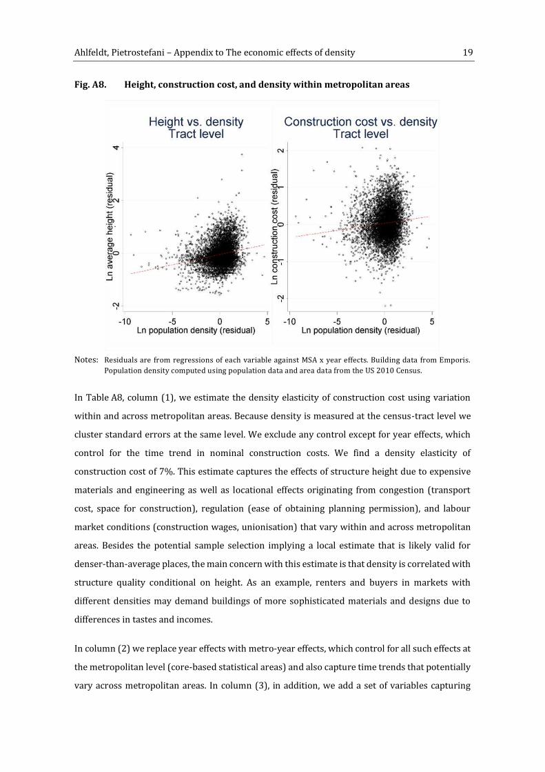
Ahlfeldt, Pietrostefani – Appendix to The economic effects of density 19
Fig. A8. Height, construction cost, and density within metropolitan areas
Notes: Residuals are from regressions of each variable against MSA x year effects. Building data from Emporis.
Population density computed using population data and area data from the US 2010 Census.
In Table A8, column (1), we estimate the density elasticity of construction cost using variation
within and across metropolitan areas. Because density is measured at the census-tract level we
cluster standard errors at the same level. We exclude any control except for year effects, which
control for the time trend in nominal construction costs. We find a density elasticity of
construction cost of 7%. This estimate captures the effects of structure height due to expensive
materials and engineering as well as locational effects originating from congestion (transport
cost, space for construction), regulation (ease of obtaining planning permission), and labour
market conditions (construction wages, unionisation) that vary within and across metropolitan
areas. Besides the potential sample selection implying a local estimate that is likely valid for
denser-than-average places, the main concern with this estimate is that density is correlated with
structure quality conditional on height. As an example, renters and buyers in markets with
different densities may demand buildings of more sophisticated materials and designs due to
differences in tastes and incomes.
In column (2) we replace year effects with metro-year effects, which control for all such effects at
the metropolitan level (core-based statistical areas) and also capture time trends that potentially
vary across metropolitan areas. In column (3), in addition, we add a set of variables capturing

Ahlfeldt, Pietrostefani – Appendix to The economic effects of density 20
non-height related features of the structure that are likely correlated with quality. Among these
variables is the ratio of building height over the number of floors, which captures the effects of
differences in ceiling height and decorative elements of the roof that primarily serve aesthetic
purposes. The controls also include two sets of variables capturing the architectural design (e.g.
modernism, postmodernism) and the structural material (e.g. wood, masonry). The density
elasticity is reduced to 4.3% conditional on these feature controls and metro-year effects. With
respect to the gross-density effect we aim to estimate, there is a concern of over-controlling (bad
control problem (Angrist & Pischke 2009)). For one thing, metro-year effects could absorb effects
related to density that vary primarily across metropolitan areas, such as labour market
conditions and regulation. For another, design and, in particular, materials (e.g. concrete and
steel) to some extent are endogenous to building height as taller buildings require different
approaches to structural engineering. In light of these concerns (omitted variable bias vs. over-
controlling) our preferred interpretation of the density elasticities reported in (1) and (3) is that
of a range between an upper-bound and a lower-bound estimate.
The remaining columns in Table A8 are added to connect to the extant literature. In column (3),
we estimate a (gross) height elasticity of construction cost of 25% for the US, which is close to the
respective elasticity estimated by Ahlfeldt & McMillen (2018) from a global sample of small
structures (up to five floors). In keeping with intuition, this elasticity decreases considerably to
approximately 14% when controlling for metro-year effects and the building features introduced
in column (3).
To our knowledge, Gyourko and Saiz (2006) provide the only explicit estimate of density effects
on construction costs that exist thus far. The estimates of the specification they use, which is
quadratic in density, imply a density elasticity of 2% at the mean of the density distribution across
US metropolitan areas. As noted above, their estimate, by construction, excludes the structure
effect as they use a construction cost index as dependent variable that refers to a same-
specification home. Their estimate also excludes various locational effects because they control
for labour market conditions and the regulatory environment. The bounds of the density effect
reported in Table A8, columns (1) and (3), thus, expectedly exceed their estimates. In column (6),
we expand the baseline model from column (1) by the feature controls from column (3) and a
large set of 310 indicator variables capturing various aspects of the building, such as the type and
the use of a building (e.g. single-family detached housing, mid-rise apartment building). We also
control for building height. With this specification, we aim to control for the structure effect as
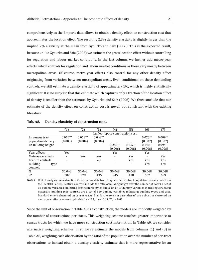
Ahlfeldt, Pietrostefani – Appendix to The economic effects of density 21
comprehensively as the Emporis data allows to obtain a density effect on construction cost that
approximates the location effect. The resulting 2.3% density elasticity is slightly larger than the
implied 2% elasticity at the mean from Gyourko and Saiz (2006). This is the expected result,
because unlike Gyourko and Saiz (2006) we estimate the gross location effect without controlling
for regulation and labour market conditions. In the last column, we further add metro-year
effects, which controls for regulation and labour market conditions as these vary mostly between
metropolitan areas. Of course, metro-year effects also control for any other density effect
originating from variation between metropolitan areas. Even conditional on these demanding
controls, we still estimate a density elasticity of approximately 1%, which is highly statistically
significant. It is no surprise that this estimate which captures only a fraction of the location effect
of density is smaller than the estimates by Gyourko and Saiz (2006). We thus conclude that our
estimate of the density effect on construction cost is novel, but consistent with the existing
literature.
Tab. A8. Density elasticity of construction costs
(1) (2) (3) (4) (5) (6) (7) Ln floor space construction cost Ln census tract population density
0.070*** (0.003)
0.053*** (0.004)
0.043*** (0.004)
0.023*** (0.002)
0.009*** (0.002)
Ln Building height
0.250*** (0.006)
0.137*** (0.008)
0.140*** (0.008)
0.094*** (0.008)
Year effects Yes - - Yes - Yes - Metro-year effects - Yes Yes - Yes - Yes Feature controls - - Yes - Yes Yes Yes Building type controls
- - - - - Yes Yes
N 30,048 30,048 30,048 30,048 30,048 30,048 30,048 r2 .202 .379 .435 .245 .438 .607 .699
Notes: Unit of analysis is construction. Construction data from Emporis. Census tract population density data from
the US 2010 Census. Feature controls include the ratio of building height over the number of floors, a set of
18 dummy variables indicating architectural styles and a set of 19 dummy variables indicating structural
materials. Building type controls are a set of 310 dummy variables indicating building types and uses.
Standard errors clustered on census tracts. Standard errors (in parentheses) are robust or clustered on
metro-year effects where applicable. * p < 0.1, ** p < 0.05, *** p < 0.01
Since the unit of observation in Table A8 is a construction, the models are implicitly weighted by
the number of constructions per tracts. This weighting scheme attaches greater importance to
census tracts for which we have more construction cost information. In Table A9, we consider
alternative weighting schemes. First, we re-estimate the models from columns (1) and (3) in
Table A8, weighting each observation by the ratio of the population over the number of per-tract
observations to instead obtain a density elasticity estimate that is more representative for an

Ahlfeldt, Pietrostefani – Appendix to The economic effects of density 22
average household (columns 1-2). Then, we repeat the exercise using the inverse of the
observation count (same weight to all tracts, columns 3-4) and the tract-population (lager
weights to tracts with many constructions and large population) as weights. The density elasticity
estimates reported in Table A8, columns (1) and (3) are roughly at the centre of the range of
estimates we find in this sensitivity analysis.
Tab. A9. Density elasticity of construction costs
(1) (2) (3) (4) (5) (6) Ln floor space construction cost
Ln census tract population density
0.088*** (0.009)
0.057*** (0.008)
0.046*** (0.003)
0.025*** (0.004)
0.073*** (0.004)
0.044*** (0.004)
Year effects Yes - Yes - Yes - Metro year effects - Yes - Yes - Yes Feature controls - Yes - Yes - Yes Building type controls
- - - - - -
Weights Tract population / Emporis count
1 / Emporis count Tract population
N 30,048 30,048 30,048 30,048 30,048 30,048 r2 .211 .441 .172 .443 .179 .412
Notes: Unit of analysis is construction. Construction data from Emporis. Census tract population density data from
the US 2010 Census. Feature controls include the ratio of building height over the number of floors, a set of
18 dummy variables indicating architectural styles and a set of 19 dummy variables indicating structural
materials. Building type controls are a set of 310 dummy variables indicating building types and uses.
Standard errors clustered on census tracts. Standard errors (in parentheses) are robust or clustered on
metro-year effects where applicable. * p < 0.1, ** p < 0.05, *** p < 0.01
2.2.2 Index-based estimates
As noted, our primary concerns with the estimation of density effects using the Emporis data are
the selectivity of the sample and an imperfect control for structural quality. These concerns
motivate a complementary analysis in which we rely on engineering estimates of construction
costs. This approach does not involve the arguably attractive use of actual micro data, but it
largely avoids the aforementioned problems.
In what follows, our aim is to estimate the cost of providing a mix of structures required to
accommodate higher density (essentially greater average building height), holding non-height
related structure features constant. While the use of an engineering cost index as dependent
variable is analogical to Gyourko and Saiz (2006), the density effect we estimate is not. Gyourko
and Saiz (2006) estimate the density effect on the cost of a same-specification home, i.e. they hold
the structure effect constant and estimate a location effect. In contrast, we focus exclusively on
the effect of having taller same-quality structures at denser places, i.e. we hold the location effect
Ahlfeldt, Pietrostefani – Appendix to The economic effects of density 23
constant and estimate the structure effect. We argue that combining both estimates yields a
reasonable approximation of the gross density effect that can be compared to our micro-data
estimates of the density elasticity.
For this exercise, we require the composition of dwelling units by structure type at a
geographically disaggregated level. To approximate the shares of various structure types we
make use of the American Community Survey (ACS). The data contains relatively rich information
on the type structure a household lives in for a 1% sample of the total US population. To increase
the number of observations we pool the 2010-2015 survey waves, weighting each observation
by the sample weight reported in the data.
As expected, the left panel of Figure A9 reveals that the great majority of households live in single-
family homes (left panel). To explore the relationship between construction cost and density, we
merge a structure-type specific per-unit construction cost index to the data. Ellis (2004) provides
same-quality per-dwelling-unit engineering estimates of relative construction cost for eight
structure types, which roughly correspond to the eight structure types in the ACS data. According
to the Ellis (2004) index illustrated in the right panel of Figure A9, same-quality-same-size units
in large multi-family structures are more than twice as expensive to build as single-family homes
because they require more expensive materials (e.g. brick), more sophisticated structural
engineering (e.g. concrete frames), and facilities (e.g. elevators).

Ahlfeldt, Pietrostefani – Appendix to The economic effects of density 24
Fig. A9. Household accommodation by structure
Notes: Left panel uses household-level data from American Community Survey (ACS), weighted by household
weights. SF = single family house, MF = multi-family house (Ruggles et al. 2017). Right panel illustrates the
construction cost index by Ellis (2004), mapping the closest of the eight categories in Ellis to each of the
eight categories in IPUMS.
Having merged the Ellis index to the ACS data by structure type, it is straightforward to compute
the weighted (by the household weight) mean structure replacement value within a public use
microdata area (PUMA) – the smallest geographic identifier in the ACS data set – to which we
refer to as construction cost for simplicity. To this PUMA level data set we merge population data
from the ACS and the geographic area from the US Census to compute density (US Census Bureau
2010).
In the left panel of Figure A10, we examine the relationship between structure composition and
density. In keeping with intuition, higher densities are associated with larger shares of units in
multi-family buildings, i.e. density is correlated with height as already evident from Figure A8.
The relationship seems to be non-linear. One interpretation is that at low levels of density,
increases in density can be achieved by building single-family homes more densely. Beyond a
certain level, however, higher densities require the construction of tall multi-family buildings.
Expectedly, the positive non-linear correlation also exists between density and the mean
construction cost (right panel).

Ahlfeldt, Pietrostefani – Appendix to The economic effects of density 25
Fig. A10. Density, dwelling type, and the cost of construction
Notes: Unit of analysis is PUMA. Ln population density rescaled to have a zero mean. Area-based construction cost
index and share of dwelling in multi-family structures is computed as the mean over the construction cost
by dwelling type provided by Ellis (2004), weighted by the dwelling-type shares in the IPUMS data
(incorporating sample weights). Population density computed using population data and area data from
the American Community Survey (ACS).
In the table below, we provide estimates of the density elasticity of our construction cost index at
the PUMA level. To account for the non-linearity suggested by Figure A10, we experiment with a
quadratic specification. We also add metro effects in some specifications and weight observations
by PUMA population in others. The elasticity estimates (at the mean) range from 4.3-5.6%. As
discussed above, these estimates capture the structure effect of density exclusively. Adding the
2% location effect estimated by Gyourko and Saiz (2006) (at the mean of the density distribution),
we obtain a combined effect in the range of 6% to 7.5%, which is close to the upper bound of the
density elasticity estimated from the micro-data. The quadratic specification from column (2)
implies a spread of the marginal density effect of 3.8-6.6% from the 5th to the 95th percentile in
the density distribution across PUMAs.

Ahlfeldt, Pietrostefani – Appendix to The economic effects of density 26
Tab. A10. Density elasticity of construction costs (index-based models)
(1) (2) (3) (4) (5) (6)
Ln construction cost index
Ln population
density
0.043***
(0.003)
0.055***
(0.004)
0.043***
(0.005)
0.056***
(0.006)
0.043***
(0.003)
0.056***
(0.005)
Ln population
density squared
0.011***
(0.002)
0.012***
(0.003)
0.012***
(0.002)
CBSA effects - - Yes Yes - Yes
Weighted - - - - By pop. By pop.
N 1158 1158 1158 1158 1158 1158
r2 .259 .323 .357 .41 .263 .417
Notes: Unit of analysis is PUMA. Ln population density rescaled to have a zero mean. Area-based construction cost
index is computed as the mean over the construction cost by dwelling type provided by Ellis (2004),
weighted by the dwelling-type shares in the ACS data (incorporating sample weights). Population density
computed using population data from ACS data and area data from US Census Bureau. Standard errors are
robust or clustered on CBSAs where included. * p < 0.1, ** p < 0.05, *** p < 0.01
2.2.3 Summary
The micro-data analysis presented in this section yields a density elasticity of construction cost
that is a composite of all structural effects (costs of building taller structures to achieve density)
and locational effects (costs of building similar structures at denser locations). However, because
of the potential selectivity of the Emporis data, the density estimate is potentially local and
representative for above-average density locations. The estimates may also confound the effects
of non-height-related structural characteristics (quality of design and materials) that are
correlated with density. Our index-based estimates are likely robust to these problems because
the composition of dwelling types in the ACS data is likely representative and the engineering
cost index we use refers to constant-quality units. However, these estimates capture exclusively
the structure effect of density, and not the location effect, for which we refer to Gyourko and Saiz
(2006).
The combined structural and locational effect that results from summing our engineering
estimate and Gyourko and Saiz (2006)’s estimate of the density elasticity still differs conceptually from the elasticity that results from the analysis of the micro-data. Gyourko and Saiz (2006)
control for several locational attributes that are likely correlated with and potentially
endogenous to density. If regulation was tighter in denser areas and had a positive effect on
construction cost (Green et al. 2005; Saiz 2010; Gyourko & Saiz 2006), one would expect the
density elasticity estimated from the micro-data to exceed the index-based elasticity (our
engineering estimate, plus Gyourko and Saiz (2006) estimate). However, the index-based
estimate is close to the upper-bound estimate from the micro-data, even though we suspect, if

Ahlfeldt, Pietrostefani – Appendix to The economic effects of density 27
anything, an upward bias of the latter due to selection. This is consistent with a weakly negative
correlation between the Wharton Regulatory Index and population density, which suggests that
achieving density is not the primary motivation for more intense regulation in the US (Gyourko
et al. 2007)
Based on the evidence presented in this section, we conclude that 4-7% is a conservative range
for the density elasticity of construction cost. This estimate is a gross estimate that includes all
structure effects and location effects that are associated with density (including differences in
regulation, geology and labour market conditions may be cause or effects of density).
2.3 Converting marginal effects into elasticities
Where possible, we convert reported marginal effects in levels or reported semi-elasticities into
density elasticities (at the mean of a distribution) using descriptive statistics reported in the
studies. Where necessary, we conduct auxiliary research into the institutional setting to facilitate
such conversions (e.g. to infer mean density). For studies from disciplines that are remote to
economics (e.g. engineering and medical research), additional steps are often required to infer
density elasticity estimates because the results are reported not as marginal density effects but
as predicted values by density category (e.g. energy consumption or adjusted premature
mortality rates). In such instances, we extract the predicted values (if necessary, by the visual
inspection of graphs) and approximate the implied density elasticity by regressing the natural
logarithm of an outcome value against the natural logarithm of the midpoint of the density
interval.
In this subsection we discuss how we adjust the density effects reported in the literature into a
consistent format. Our aim is to express as many as possible estimates in terms of an elasticity of
an outcome measure Y with respect to density P/A:
𝛽 = 𝑑𝑌𝑌𝑑(𝑃/𝐴)(𝑃/𝐴)
, where P (population) and A (area) are defined as in the previous sub-section. Authors of the
studies included in the evidence base frequently report marginal effects of the following forms:
Marginal effects in levels:
Ahlfeldt, Pietrostefani – Appendix to The economic effects of density 28
𝛾 = 𝑑𝑌𝑑(𝑃/𝐴)
Log-lin semi-elasticities estimated using log-lin models:
𝛿 = 𝑑𝑌𝑌𝑑(𝑃/𝐴)
Lin-log semi-elasticities estimated using lin-log models:
𝜗 = 𝑑𝑌𝑑 (𝑃𝐴)(𝑃/𝐴)
Hence, we can compute 𝛽 at the mean of the distributions of Y and P (denoted by bars) from
reported estimates of 𝛾 or 𝛿 or 𝜗 as follows:
𝛽 = 𝛿(𝑃/𝐴̅̅ ̅̅ ̅̅ )
𝛽 = 𝛾 (𝑃/𝐴̅̅ ̅̅ ̅̅ )�̅�
𝛽 = 𝜗 1�̅�
We note that in some instances, a conversion into an elasticity requires further auxiliary steps
such as removing a standardisation (normalisation by standard deviations) or the auxiliary
estimation of elasticities based on results reported for discrete categories. In some cases, we infer
a marginal effect from graphical illustrations (in particular in the health category).
2.4 Converting city size elasticities into density elasticities
In several instances the authors of the considered analyses use city population as a proxy of
density. The elasticity of an outcome with respect to population (city size proxy) takes the
following form (after the transformations described 2.2, if necessary):
𝜃 = 𝑑𝑌𝑌𝑑(𝑃)(𝑃)
As we have shown in 2.1, the elasticity of density with respect to city size is not unity. It is
therefore necessary to adjust the estimates in order to make them comparable to elasticities with
Ahlfeldt, Pietrostefani – Appendix to The economic effects of density 29
respect to density. Given that we have an estimate of the elasticity of density with respect to city
size
𝛼 = 𝑑(𝑃/𝐴)(𝑃/𝐴)𝑑𝑃𝑃
we can easily compute the elasticity of an outcome with respect to density as:
𝛽 = 𝜃𝛼
2.5 Converting density elasticities of land price into density
elasticities of rent
Density effects on the value of real estate are often reported in terms of house price capitalisation,
which is linearly related to rent capitalisation (assuming a constant discount factor). Sometimes,
authors report the effects in terms of land price capitalisation. Land price elasticities are not
directly comparable to house price elasticities because house prices generally move less than land
prices due to factor substitution (developers substitute away from land as land prices increase).
To allow for a simple micro-founded translation of land price capitalisation effects into house
price capitalisation effects, it is useful to assume a Cobb-Douglas housing production function and
a competitive construction sector. Assume that housing services H are produced using the inputs
capital K and land L as follows: 𝐻 = 𝐾ℶ𝐿1−ℶ. Housing space is rented out at bid-rent 𝜓 while land
is acquired at land rent Ω. From the first-order condition 𝐾/𝐿 = ℶ/(1 − ℶ) Ω (the price of capital
is the numeraire) and the non-profit condition 𝜓𝐻 = 𝐾 + Ω𝐿, it is immediate that log(𝜓) =(1 − ℶ) log(Ω) + 𝑐, where c is a constant that cancels out in differences, i.e., 𝑑 ln(𝜓) =(1 − ℶ)𝑑 ln(𝛺).
It is, therefore, possible to translate an elasticity of land price with respect to density into an
elasticity of rent (house price) with respect to density as follows: 𝑑 ln 𝜓𝑑ln (𝑃𝐴) = (1 − ℶ) 𝑑 ln 𝛺𝑑ln (𝑃𝐴)
, where we set (1 − ℶ) = 0.25, following Ahlfeldt et al. (2015).
Ahlfeldt, Pietrostefani – Appendix to The economic effects of density 30
2.6 Density elasticities: High-income vs. non-high-income
In the table below, we compare citation-weighted median and mean elasticities between high-
income countries and non-high-income countries. The table complements Table 3 in the main
paper. Evidently, the evidence base from non-high-income countries is limited. Notably we
observe that mean elasticities differ between high-income and non-high-income countries in
outcome categories where we are able to observe this. For productivity, the unconditional
citation-weighted mean in the evidence base is 0.08 for non-high-income countries, while 0.04
for high income countries. Within the quality of life category, we also observe that while density
has an average positive effect on quality of life in high-income places, it has an average negative
effect in non-high-income countries. Another relevant finding is that the density elasticities of
non-car use are significantly lower for non-high-income countries.
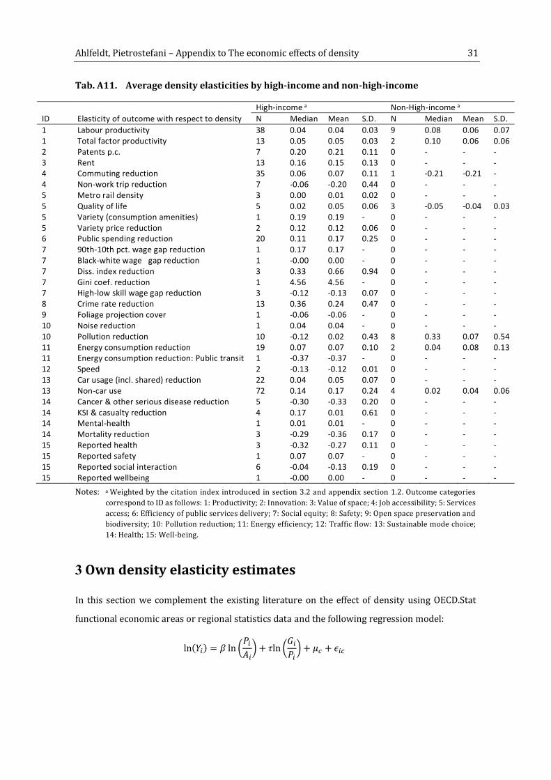
Ahlfeldt, Pietrostefani – Appendix to The economic effects of density 31
Tab. A11. Average density elasticities by high-income and non-high-income
High-income a Non-High-income a
ID Elasticity of outcome with respect to density N Median Mean S.D. N Median Mean S.D.
1 Labour productivity 38 0.04 0.04 0.03 9 0.08 0.06 0.07
1 Total factor productivity 13 0.05 0.05 0.03 2 0.10 0.06 0.06
2 Patents p.c. 7 0.20 0.21 0.11 0 - - -
3 Rent 13 0.16 0.15 0.13 0 - - -
4 Commuting reduction 35 0.06 0.07 0.11 1 -0.21 -0.21 -
4 Non-work trip reduction 7 -0.06 -0.20 0.44 0 - - -
5 Metro rail density 3 0.00 0.01 0.02 0 - - -
5 Quality of life 5 0.02 0.05 0.06 3 -0.05 -0.04 0.03
5 Variety (consumption amenities) 1 0.19 0.19 - 0 - - -
5 Variety price reduction 2 0.12 0.12 0.06 0 - - -
6 Public spending reduction 20 0.11 0.17 0.25 0 - - -
7 90th-10th pct. wage gap reduction 1 0.17 0.17 - 0 - - -
7 Black-white wage gap reduction 1 -0.00 0.00 - 0 - - -
7 Diss. index reduction 3 0.33 0.66 0.94 0 - - -
7 Gini coef. reduction 1 4.56 4.56 - 0 - - -
7 High-low skill wage gap reduction 3 -0.12 -0.13 0.07 0 - - -
8 Crime rate reduction 13 0.36 0.24 0.47 0 - - -
9 Foliage projection cover 1 -0.06 -0.06 - 0 - - -
10 Noise reduction 1 0.04 0.04 - 0 - - -
10 Pollution reduction 10 -0.12 0.02 0.43 8 0.33 0.07 0.54
11 Energy consumption reduction 19 0.07 0.07 0.10 2 0.04 0.08 0.13
11 Energy consumption reduction: Public transit 1 -0.37 -0.37 - 0 - - -
12 Speed 2 -0.13 -0.12 0.01 0 - - -
13 Car usage (incl. shared) reduction 22 0.04 0.05 0.07 0 - - -
13 Non-car use 72 0.14 0.17 0.24 4 0.02 0.04 0.06
14 Cancer & other serious disease reduction 5 -0.30 -0.33 0.20 0 - - -
14 KSI & casualty reduction 4 0.17 0.01 0.61 0 - - -
14 Mental-health 1 0.01 0.01 - 0 - - -
14 Mortality reduction 3 -0.29 -0.36 0.17 0 - - -
15 Reported health 3 -0.32 -0.27 0.11 0 - - -
15 Reported safety 1 0.07 0.07 - 0 - - -
15 Reported social interaction 6 -0.04 -0.13 0.19 0 - - -
15 Reported wellbeing 1 -0.00 0.00 - 0 - - -
Notes: a Weighted by the citation index introduced in section 3.2 and appendix section 1.2. Outcome categories
correspond to ID as follows: 1: Productivity; 2: Innovation: 3: Value of space; 4: Job accessibility; 5: Services
access; 6: Efficiency of public services delivery; 7: Social equity; 8: Safety; 9: Open space preservation and
biodiversity; 10: Pollution reduction; 11: Energy efficiency; 12: Traffic flow: 13: Sustainable mode choice;
14: Health; 15: Well-being.
3 Own density elasticity estimates
In this section we complement the existing literature on the effect of density using OECD.Stat
functional economic areas or regional statistics data and the following regression model:
ln(𝑌𝑖) = 𝛽 ln (𝑃𝑖𝐴𝑖) + 𝜏ln (𝐺𝑖𝑃𝑖 ) + 𝜇𝑐 + 𝜖𝑖𝑐
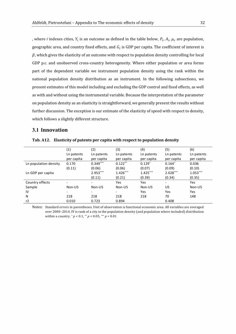
Ahlfeldt, Pietrostefani – Appendix to The economic effects of density 32
, where i indexes cities, 𝑌𝑖 is an outcome as defined in the table below, 𝑃𝑖 , 𝐴𝑖 , 𝜇𝑐 are population,
geographic area, and country fixed effects, and 𝐺𝑖 is GDP per capita. The coefficient of interest is 𝛽, which gives the elasticity of an outcome with respect to population density controlling for local
GDP p.c. and unobserved cross-country heterogeneity. Where either population or area forms
part of the dependent variable we instrument population density using the rank within the
national population density distribution as an instrument. In the following subsections, we
present estimates of this model including and excluding the GDP control and fixed effects, as well
as with and without using the instrumental variable. Because the interpretation of the parameter
on population density as an elasticity is straightforward, we generally present the results without
further discussion. The exception is our estimate of the elasticity of speed with respect to density,
which follows a slightly different structure.
3.1 Innovation
Tab. A12. Elasticity of patents per capita with respect to population density
(1) (2) (3) (4) (5) (6)
Ln patents
per capita
Ln patents
per capita
Ln patents
per capita
Ln patents
per capita
Ln patents
per capita
Ln patents
per capita
Ln population density 0.170
(0.11)
0.349***
(0.06)
0.122**
(0.06)
0.129*
(0.07)
0.164*
(0.09)
0.036
(0.10)
Ln GDP per capita
2.953***
(0.11)
1.426***
(0.21)
1.425***
(0.39)
2.028***
(0.34)
1.053***
(0.35)
Country effects - - Yes Yes - Yes
Sample Non-US Non-US Non-US Non-US US Non-US
IV - - - Yes Yes Yes
N 218 218 218 218 70 148
r2 0.010 0.723 0.894 0.408
Notes: Standard errors in parentheses. Unit of observation is functional economic area. All variables are averaged
over 2000–2014. IV is rank of a city in the population density (and population where included) distribution
within a country. * p < 0.1, ** p < 0.05, *** p < 0.01

Ahlfeldt, Pietrostefani – Appendix to The economic effects of density 33
3.2 Services access (broadband)
Tab. A13. Elasticity of broadband per capita with respect to population density
(1) (2) (3) (4) (5) (6)
Ln
broadband
per capita
Ln
broadband
per capita
Ln
broadband
per capita
Ln
broadband
per capita
Ln
broadband
per capita
Ln
broadband
per capita
Ln population density 0.033***
(0.01)
0.034***
(0.01)
0.011
(0.01)
0.010
(0.01)
-0.000
(0.00)
0.013
(0.01)
Ln GDP per capita
0.474***
(0.04)
0.305***
(0.06)
0.306***
(0.06)
0.119
(0.07)
0.327***
(0.06)
Country effects - - Yes Yes - Yes
IV - - - Yes Yes Yes
N 343 343 343 343 51 292
Sample All All All All US Non-US
r2 0.020 0.576 0.862 0.186
Notes: Standard errors in parentheses. Unit of observation is large regions (OECD definition). All variables are
averaged over 2000–2014. IV is rank of a city in the population density distribution within a country. * p <
0.1, ** p < 0.05, *** p < 0.01
3.3 Social equity
Tab. A14. Elasticity of income quintile ratio with respect to population density
(1) (2) (3) (4) (5)
Ln disposable
income
quintile ratio
(pct. 80 vs
20)
Ln disposable
income
quintile ratio
(pct. 80 vs
20)
Ln disposable
income
quintile ratio
(pct. 80 vs
20)
Ln disposable
income
quintile ratio
(pct. 80 vs
20)
Ln disposable
income
quintile ratio
(pct. 80 vs
20)
Ln population density 0.023
(0.02)
0.024
(0.03)
0.035**
(0.01)
0.057***
(0.02)
0.032**
(0.01)
Ln GDP per capita
-0.233***
(0.09)
0.469
(0.29)
0.197*
(0.11)
0.503
(0.32)
Country effects - - Yes - Yes
IV - - - - -
N 275 269 269 51 218
Sample All All All US Non-US
r2 0.004 0.042 0.734 0.352 0.718
Notes: Standard errors in parentheses. Unit of observation is large regions (OECD definition). All variables are
averaged over 2000–2014. * p < 0.1, ** p < 0.05, *** p < 0.01
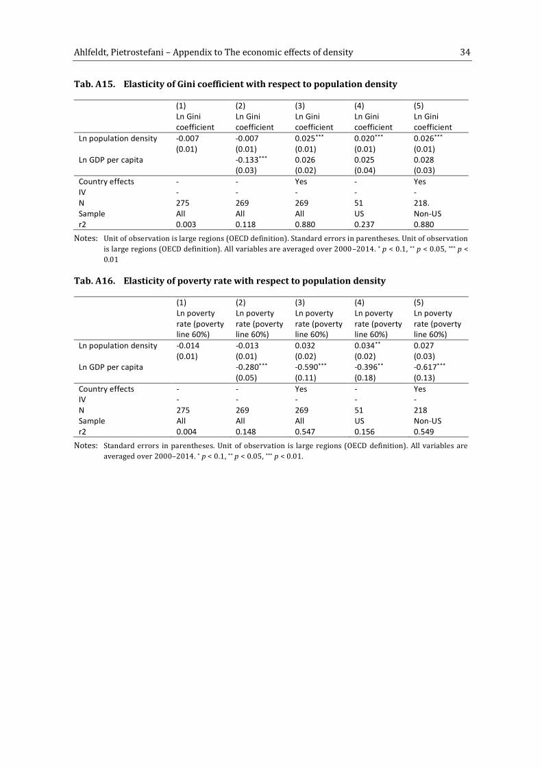
Ahlfeldt, Pietrostefani – Appendix to The economic effects of density 34
Tab. A15. Elasticity of Gini coefficient with respect to population density
(1) (2) (3) (4) (5)
Ln Gini
coefficient
Ln Gini
coefficient
Ln Gini
coefficient
Ln Gini
coefficient
Ln Gini
coefficient
Ln population density -0.007
(0.01)
-0.007
(0.01)
0.025***
(0.01)
0.020***
(0.01)
0.026***
(0.01)
Ln GDP per capita
-0.133***
(0.03)
0.026
(0.02)
0.025
(0.04)
0.028
(0.03)
Country effects - - Yes - Yes
IV - - - - -
N 275 269 269 51 218.
Sample All All All US Non-US
r2 0.003 0.118 0.880 0.237 0.880
Notes: Unit of observation is large regions (OECD definition). Standard errors in parentheses. Unit of observation
is large regions (OECD definition). All variables are averaged over 2000–2014. * p < 0.1, ** p < 0.05, *** p <
0.01
Tab. A16. Elasticity of poverty rate with respect to population density
(1) (2) (3) (4) (5)
Ln poverty
rate (poverty
line 60%)
Ln poverty
rate (poverty
line 60%)
Ln poverty
rate (poverty
line 60%)
Ln poverty
rate (poverty
line 60%)
Ln poverty
rate (poverty
line 60%)
Ln population density -0.014
(0.01)
-0.013
(0.01)
0.032
(0.02)
0.034**
(0.02)
0.027
(0.03)
Ln GDP per capita
-0.280***
(0.05)
-0.590***
(0.11)
-0.396**
(0.18)
-0.617***
(0.13)
Country effects - - Yes - Yes
IV - - - - -
N 275 269 269 51 218
Sample All All All US Non-US
r2 0.004 0.148 0.547 0.156 0.549
Notes: Standard errors in parentheses. Unit of observation is large regions (OECD definition). All variables are
averaged over 2000–2014. * p < 0.1, ** p < 0.05, *** p < 0.01.

Ahlfeldt, Pietrostefani – Appendix to The economic effects of density 35
3.4 Safety
Tab. A17. Elasticity of homicides p.c. with respect to population density
(1) (2) (3) (4) (5) (6)
Ln
homicides
p.c.
Ln
homicides
p.c.
Ln
homicides
p.c.
Ln
homicides
p.c.
Ln
homicides
p.c.
Ln
homicides
p.c.
Ln population density -0.204***
(0.03)
-0.166***
(0.03)
-0.033
(0.04)
-0.048
(0.04)
0.105**
(0.05)
-0.076**
(0.04)
Ln GDP per capita
-0.918***
(0.07)
0.086
(0.06)
0.086
(0.07)
0.312
(0.48)
0.058
(0.07)
Country effects - - Yes Yes - Yes
IV - - - Yes Yes Yes
N 481 474 474 474 51 423
Sample All All All All US Non-US
r2 0.088 0.393 0.879 0.139
Notes: Standard errors in parentheses. Unit of observation is large regions (OECD definition). All variables are
averaged over 2000–2014. IV is rank of a city in the population density distribution within a country. * p <
0.1, ** p < 0.05, *** p < 0.01.
3.5 Urban green
Tab. A18. Elasticity of vegetation density with respect to population density
(1) (2) (3) (4) (5) (6)
Ln
vegetation
density
Ln
vegetation
density
Ln
vegetation
density
Ln
vegetation
density
Ln
vegetation
density
Ln
vegetation
density
Ln population density -0.199***
(0.02)
-0.267***
(0.02)
-0.257***
(0.04)
-0.245***
(0.05)
0.034
(0.10)
-0.261***
(0.05)
Ln GDP per capita
0.388***
(0.06)
Country effects - - Yes Yes - Yes
IV - - - Yes Yes Yes
N 583 410 583 583 45 538
Sample All Non-US All All US Non-US
r2 0.142 0.262 0.381
Notes: Standard errors in parentheses. Unit of observation is small regions (urban and intermediate, OECD
definition). US GDP data not available at this scale. All variables are averaged over 2000–2014. IV is rank of
a city in the population density distribution within a country. * p < 0.1, ** p < 0.05, *** p < 0.01

Ahlfeldt, Pietrostefani – Appendix to The economic effects of density 36
Tab. A19. Elasticity of green area density with respect to population density
(1) (2) (3) (4) (5) (6)
Ln green
area density
Ln green
area density
Ln green
area density
Ln green
area density
Ln green
area density
Ln green
area density
Ln population density 0.283**
(0.14)
0.683**
(0.31)
0.761*
(0.40)
1.446***
(0.38)
0.197
(0.43)
Ln GDP per capita
0.496**
(0.23)
0.035
(0.94)
0.022
(0.86)
1.178
(0.96)
-0.857
(0.69)
Country effects - - Yes Yes - Yes
IV - - - Yes Yes Yes
N 280 280 280 280 70 210
Sample All All All All US Non-US
r2 0.021 0.040 0.283 0.246
Notes: Standard errors in parentheses. Unit of observation is functional economic area. All variables are averaged
over 2000–2014. IV is rank of a city in the population density (and population where included) distribution
within a country. * p < 0.1, ** p < 0.05, *** p < 0.01
Tab. A20. Elasticity of green area per capita with respect to population density
(1) (2) (3) (4) (5) (6)
Ln green
area per
capita
Ln green
area per
capita
Ln green
area per
capita
Ln green
area per
capita
Ln green
area per
capita
Ln green
area per
capita
Ln population density -0.754***
(0.14)
-0.717***
(0.14)
-0.317
(0.31)
-0.239
(0.40)
0.446
(0.38)
-0.803*
(0.43)
Ln GDP per capita
0.496**
(0.23)
0.035
(0.94)
0.022
(0.86)
1.178
(0.96)
-0.857
(0.69)
Country effects - - Yes Yes - Yes
IV - - - Yes Yes Yes
N 280 280 280 280 70 210
Sample All All All All US Non-US
r2 0.170 0.186 0.392 0.027
Notes: Standard errors in parentheses. Unit of observation is functional economic area. All variables are averaged
over 2000–2014. IV is rank of a city in the population density (and population where included) distribution
within a country. * p < 0.1, ** p < 0.05, *** p < 0.01

Ahlfeldt, Pietrostefani – Appendix to The economic effects of density 37
3.6 Pollution concentration
Tab. A21. Elasticity of air pollution concentration with respect to population density
(1) (2) (3) (4) (5)
Ln air
pollution
(level PM2.5)
Ln air
pollution
(level PM2.5)
Ln air
pollution
(level PM2.5)
Ln air
pollution
(level PM2.5)
Ln air
pollution
(level PM2.5)
Ln population density 0.221***
(0.02)
0.220***
(0.02)
0.124***
(0.03)
0.111***
(0.03)
0.128***
(0.03)
Ln GDP per capita
-0.208***
(0.04)
0.020
(0.19)
0.053
(0.14)
0.018
(0.21)
Country effects - - Yes - Yes
IV - - - - -
N 343 343 343 51 292
Sample All All All US Non-US
r2 0.407 0.456 0.708 0.247 0.720
Notes: Standard errors in parentheses. Unit of observation is large regions (OECD definition). All variables are
averaged over 2000–2014. IV is rank of a city in the population density distribution within a country. * p <
0.1, ** p < 0.05, *** p < 0.01
3.7 Energy
Tab. A22. Elasticity of ln CO2 emissions p.c. with respect to population density
(1) (2) (3) (4) (5) (6)
Ln CO2
emissions
p.c.
Ln CO2
emissions
p.c.
Ln CO2
emissions
p.c.
Ln CO2
emissions
p.c.
Ln CO2
emissions
p.c.
Ln CO2
emissions
p.c.
Ln population density -0.225***
(0.02)
-0.224***
(0.02)
-0.189***
(0.04)
-0.173***
(0.04)
-0.190***
(0.05)
-0.170***
(0.05)
Ln GDP per capita
0.503***
(0.04)
0.283***
(0.08)
0.282***
(0.07)
0.354
(0.27)
0.280***
(0.07)
Country effects - - Yes Yes - Yes
IV - - - Yes Yes Yes
N 570 562 562 562 51 511
Sample All All All All US Non-US
r2 0.176 0.358 0.597 0.300
Notes: Standard errors in parentheses. Unit of observation is large urban regions (OECD definition). All variables
are averaged over 2000–2014. IV is rank of a city in the population density distribution within a country. *
p < 0.1, ** p < 0.05, *** p < 0.01
3.8 Traffic flow
In the figure below we compare the peak time (with congestion) speeds on freeways and arterial
roads across metros that are above and below the median population density. Both distributions
seem to suggest that metros with a higher population density have lower average speeds, which
is in line with more congestion in denser cities.

Ahlfeldt, Pietrostefani – Appendix to The economic effects of density 38
Fig. A11. Distribution of peak time speeds by population density
Notes: Data from OECD (population density) and Lomax (2010).
However, regressing the freeway speed against population density does not yield a significant
relationship during peak time (with congestion) or off-peak time (free flow). There is also no
population density effect on congestions, i.e., on peak time speeds controlling for free-flow
speeds. There is, however, a significantly negative effect of population size on congestion,
suggesting that freeway congestion is determined by the size of the city and not its density.
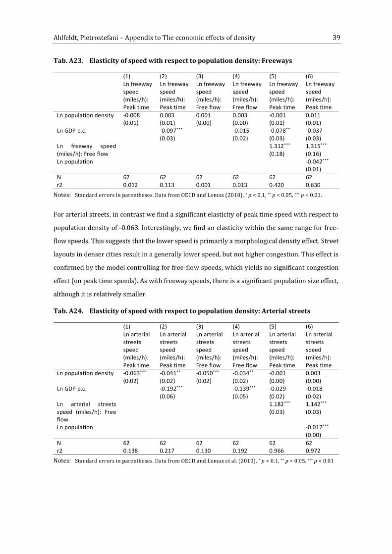
Ahlfeldt, Pietrostefani – Appendix to The economic effects of density 39
Tab. A23. Elasticity of speed with respect to population density: Freeways
(1) (2) (3) (4) (5) (6)
Ln freeway
speed
(miles/h):
Peak time
Ln freeway
speed
(miles/h):
Peak time
Ln freeway
speed
(miles/h):
Free flow
Ln freeway
speed
(miles/h):
Free flow
Ln freeway
speed
(miles/h):
Peak time
Ln freeway
speed
(miles/h):
Peak time
Ln population density -0.008
(0.01)
0.003
(0.01)
0.001
(0.00)
0.003
(0.00)
-0.001
(0.01)
0.011
(0.01)
Ln GDP p.c.
-0.097***
(0.03)
-0.015
(0.02)
-0.078**
(0.03)
-0.037
(0.03)
Ln freeway speed
(miles/h): Free flow
1.312***
(0.18)
1.315***
(0.16)
Ln population
-0.042***
(0.01)
N 62 62 62 62 62 62
r2 0.012 0.113 0.001 0.013 0.420 0.630
Notes: Standard errors in parentheses. Data from OECD and Lomax (2010). * p < 0.1, ** p < 0.05, *** p < 0.01.
For arterial streets, in contrast we find a significant elasticity of peak time speed with respect to
population density of -0.063. Interestingly, we find an elasticity within the same range for free-
flow speeds. This suggests that the lower speed is primarily a morphological density effect. Street
layouts in denser cities result in a generally lower speed, but not higher congestion. This effect is
confirmed by the model controlling for free-flow speeds, which yields no significant congestion
effect (on peak time speeds). As with freeway speeds, there is a significant population size effect,
although it is relatively smaller.
Tab. A24. Elasticity of speed with respect to population density: Arterial streets
(1) (2) (3) (4) (5) (6)
Ln arterial
streets
speed
(miles/h):
Peak time
Ln arterial
streets
speed
(miles/h):
Peak time
Ln arterial
streets
speed
(miles/h):
Free flow
Ln arterial
streets
speed
(miles/h):
Free flow
Ln arterial
streets
speed
(miles/h):
Peak time
Ln arterial
streets
speed
(miles/h):
Peak time
Ln population density -0.063***
(0.02)
-0.041**
(0.02)
-0.050***
(0.02)
-0.034**
(0.02)
-0.001
(0.00)
0.003
(0.00)
Ln GDP p.c.
-0.192***
(0.06)
-0.139***
(0.05)
-0.029
(0.02)
-0.018
(0.02)
Ln arterial streets
speed (miles/h): Free
flow
1.182***
(0.03)
1.142***
(0.03)
Ln population
-0.017***
(0.00)
N 62 62 62 62 62 62
r2 0.138 0.217 0.130 0.192 0.966 0.972
Notes: Standard errors in parentheses. Data from OECD and Lomax et al. (2010). * p < 0.1, ** p < 0.05, *** p < 0.01
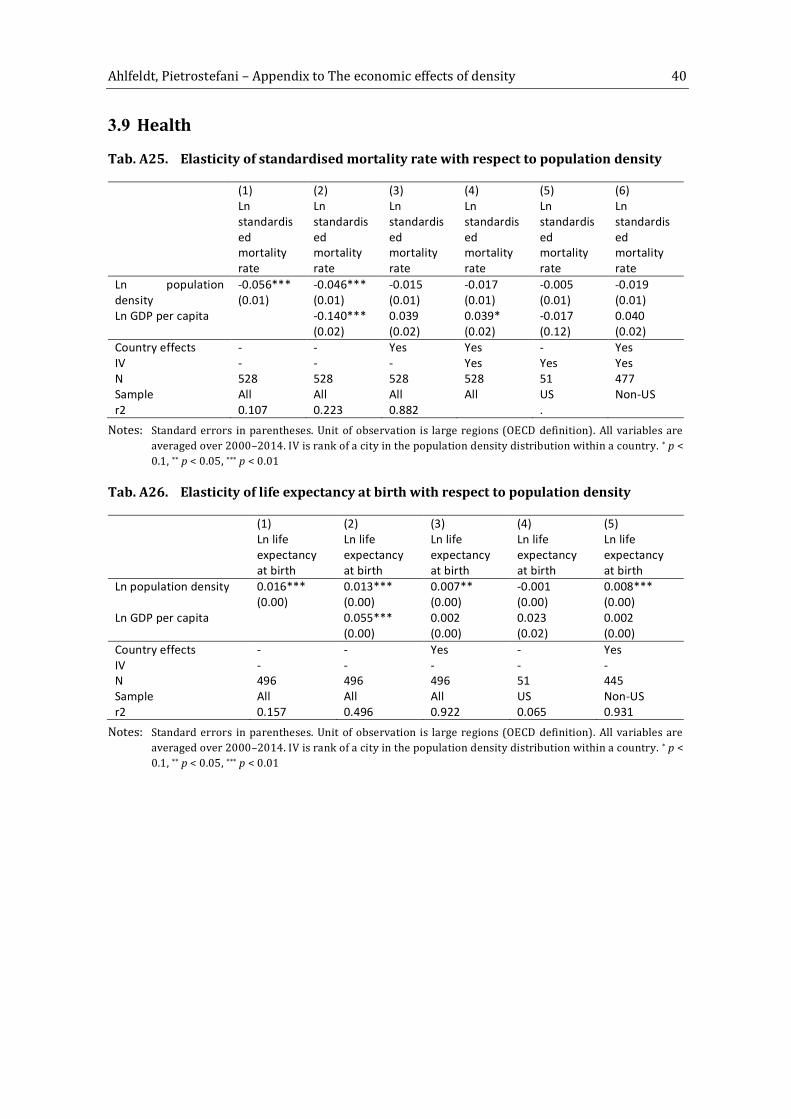
Ahlfeldt, Pietrostefani – Appendix to The economic effects of density 40
3.9 Health
Tab. A25. Elasticity of standardised mortality rate with respect to population density
(1) (2) (3) (4) (5) (6)
Ln
standardis
ed
mortality
rate
Ln
standardis
ed
mortality
rate
Ln
standardis
ed
mortality
rate
Ln
standardis
ed
mortality
rate
Ln
standardis
ed
mortality
rate
Ln
standardis
ed
mortality
rate
Ln population
density
-0.056***
(0.01)
-0.046***
(0.01)
-0.015
(0.01)
-0.017
(0.01)
-0.005
(0.01)
-0.019
(0.01)
Ln GDP per capita
-0.140***
(0.02)
0.039
(0.02)
0.039*
(0.02)
-0.017
(0.12)
0.040
(0.02)
Country effects - - Yes Yes - Yes
IV - - - Yes Yes Yes
N 528 528 528 528 51 477
Sample All All All All US Non-US
r2 0.107 0.223 0.882 .
Notes: Standard errors in parentheses. Unit of observation is large regions (OECD definition). All variables are
averaged over 2000–2014. IV is rank of a city in the population density distribution within a country. * p <
0.1, ** p < 0.05, *** p < 0.01
Tab. A26. Elasticity of life expectancy at birth with respect to population density
(1) (2) (3) (4) (5)
Ln life
expectancy
at birth
Ln life
expectancy
at birth
Ln life
expectancy
at birth
Ln life
expectancy
at birth
Ln life
expectancy
at birth
Ln population density 0.016***
(0.00)
0.013***
(0.00)
0.007**
(0.00)
-0.001
(0.00)
0.008***
(0.00)
Ln GDP per capita
0.055***
(0.00)
0.002
(0.00)
0.023
(0.02)
0.002
(0.00)
Country effects - - Yes - Yes
IV - - - - -
N 496 496 496 51 445
Sample All All All US Non-US
r2 0.157 0.496 0.922 0.065 0.931
Notes: Standard errors in parentheses. Unit of observation is large regions (OECD definition). All variables are
averaged over 2000–2014. IV is rank of a city in the population density distribution within a country. * p <
0.1, ** p < 0.05, *** p < 0.01

Ahlfeldt, Pietrostefani – Appendix to The economic effects of density 41
Tab. A27. Elasticity of mortality in transport p.c. with respect to population density
(1) (2) (3) (4) (5) (6)
Ln
mortality
in
transport
p.c.
Ln
mortality
in
transport
p.c.
Ln
mortality
in
transport
p.c.
Ln
mortality
in
transport
p.c.
Ln
mortality
in
transport
p.c.
Ln
mortality
in
transport
p.c.
Ln population
density
-0.162***
(0.02)
-0.150***
(0.01)
-0.103***
(0.03)
-0.099***
(0.03)
-0.119***
(0.02)
-0.093***
(0.03)
Ln GDP per capita
-0.278***
(0.04)
-0.111**
(0.04)
-0.110***
(0.04)
-0.484*
(0.25)
-0.087**
(0.04)
Country effects - - Yes Yes - Yes
IV - - - Yes Yes Yes
N 420 414 414 414 51 363
Sample All All All All US Non-US
r2 0.260 0.375 0.819 0.534
Notes: Standard errors in parentheses. Unit of observation is large regions (OECD definition). All variables are
averaged over 2000–2014. IV is rank of a city in the population density distribution within a country. * p <
0.1, ** p < 0.05, *** p < 0.01
3.10 Well-being
Tab. A28. Elasticity of subjective well-being with respect to population density
(1) (2) (3) (4) (5)
Ln subjective
life
satisfaction
Ln subjective
life
satisfaction
Ln subjective
life
satisfaction
Ln subjective
life
satisfaction
Ln subjective
life
satisfaction
Ln population density -0.021***
(0.00)
-0.023***
(0.00)
-0.007**
(0.00)
-0.001
(0.01)
-0.008**
(0.00)
Ln GDP per capita
0.114***
(0.01)
0.069***
(0.01)
0.012
(0.04)
0.074***
(0.01)
Country effects - - Yes - Yes
IV - - - - -
N 339 339 339 51 288
Sample All All All US Non-US
r2 0.073 0.410 0.850 0.003 0.859
Notes: Standard errors in parentheses. All variables are averaged over 2000–2014. IV is rank of a city in the
population density distribution within a country. * p < 0.1, ** p < 0.05, *** p < 0.01
4 Recommended elasticities
This section provides a justification of the recommended elasticities reported in Table 5 in the
main paper alongside a critical discussion of the quality and the quantity of the evidence base. We
strongly advise consulting the relevant subsections below before applying one of the
recommended elasticities in further research.
Before we proceed to the discussion of the category-specific density elasticities, we wish to
remind the reader, that, as discussed in Section 2.1 in the main paper, there is fundamental

Ahlfeldt, Pietrostefani – Appendix to The economic effects of density 42
problem in identifying density effects because density is endogenous and potentially determined
by unobserved location fundamental factors (e.g. a favourable geography). Studies that estimate
density effects from plausibly exogenous variation (e.g. by making use of natural experiments or
instrumental variables) are the minority. For most estimates, the causal interpretation rests on
the assumption that the variation in density within and between cities is largely historically
determined by factors that have limited contemporaneous effects on outcomes. For individual-,
firm-, and unit-based outcomes (e.g. wages, innovation, rent, wellbeing), the collected density
elasticities often capture composition effects. In this case, a density elasticity does not give the
effect of an exogenous change in density on an outcome such as the productivity of individuals,
the innovative activity of firms, or the value of housing units. For individual- and firm- based
outcomes, the density elasticity, in addition, captures the composition effect that usually arises
because more productive individuals and firms self-select into more productive areas. The
density elasticity of rent captures the effect of a change in the quality of housing stock if
developers make choices that depend on rents and incomes, which in turn depend on density.
4.1 Wage elasticity
The literature reports both wage and TFP elasticities with respect to density, the former being by
far the most frequently reported parameter. While we find a significant difference between the
wage and the TFP elasticity in our review, it is notable that high quality papers analysing both
wage and TFP within a consistent framework do not report the existence of such a difference
(Combes et al. 2010). We choose the citation-weighted average value of the wage elasticities in
our sample of 0.04, which is close to the results from recent high-quality work (Combes et al.
2012) and meta-analysis (Melo et al. 2009). While there is some variation in the estimated density
elasticities of wage and TFP, the estimates in the literature do not appear to be systematically
related to the average density level in the considered study areas. However, it is noteworthy that,
within the admittedly smaller sample of studies from non-high-income countries, the citation-
weighted average of the density elasticity of wages, at 0.08, is about twice as large. We also note
that there is a tendency for within-city analyses (Ahlfeldt et al. 2015) and TFP analyses to yield
larger estimated elasticities, but we recommend further work to substantiate this impression. An
important qualification is that the recommended 0.04 elasticity is best interpreted as an area-
based effect that partially captures a productivity effect on identical workers and particle
captures a shift in composition towards more productive workers (a sorting effect). Studies that
control for unobserved heterogeneity of workers by identifying from movers across

Ahlfeldt, Pietrostefani – Appendix to The economic effects of density 43
agglomerations tend to find elasticities that are about 50% lower (Combes & Gobillon, 2015). We
recommend the 0.04 elasticity as an area-based effect that is consistent with the area-based
estimates recommended for the other categories, for which estimates controlling for unobserved
micro-level heterogeneity are typically not available.
4.2 Patents
While there is a sizeable literature engaged with the effects of urban form on innovation, we only
found seven studies that provided estimates that either directly corresponded to or could be
converted into an elasticity of patents with respect to density. Some studies report marginal
effects that cannot be converted into elasticities due to missing descriptive statistics. We
recommend the citation-weighted mean in the evidence base of 0.21, which is in line with Carlino
et al. (2007) and our own analysis of US FUAs. This consistency is reassuring. However, the
evidence base is relatively thin and our own elasticity estimates for the world-wide sample, at
0.13, are somewhat smaller than the recommended elasticity. More work aiming at comparable
elasticity estimates from different geographic contexts would be desirable.
4.3 Rents
We recommend the citation-weighted mean elasticity from the evidence base of 0.15. This
estimate is almost identical to the density elasticity of rent in the data set used by Albouy & Lue,
(2015), which was kindly provided by the authors. This estimate is also within the range of other
good quality and relevant papers. We are thus reasonably confident in recommending this
elasticity as an average even though the evidence base is not as well developed as it is, for
example, for wages. It is important to note, however, that the density elasticity of rent appears to
vary in density. Our meta-analysis of the reviewed elasticities suggests that elasticity increases
by 0.06 if the population density in the considered study area increases by 1000 inhabitants per
square kilometer. This effect is qualitatively and quantitatively consistent with the positive effect
of city size on the density elasticity of rent documented by Combes et al (2018) for French cities.
The non-log-linearity in the effect of density on rent also explains why Combes et al (2018) find
a larger elasticity for French cities than Albouy and Lue (2015) find for US cities. The 0.06
difference in the density elasticity (0.21 for French cities vs. 0.15 for US cities) corresponds to a
difference in density of about 1000 inhabitants per square kilometer, almost exactly the
difference reported in the Demographia World Urban Areas (2018).

Ahlfeldt, Pietrostefani – Appendix to The economic effects of density 44
4.4 Vehicle miles travelled
We recommend the citation-weighted mean elasticity from the evidence base of 0.06. The
evidence base, including 36 analyses, is relatively large. There is sizeable variation in the
estimated density elasticity across analyses (standard deviation of 0.12). Our recommended
elasticity, however, is relatively close to Duranton & Turner (2018), a dedicated high-quality
paper, and to the mean elasticity recommended in the meta-analysis (0.04) by Ewing & Cervero
(2010). We are therefore reasonably confident in recommending this elasticity, even though
there is significant heterogeneity that remains to be explored.
4.5 Variety benefits
The literature on consumption benefits arising from agglomeration is underdeveloped relative to
the production side. However, there are some good papers which suggest a sizeable effect. Victor
Couture kindly provided estimates of the elasticity of restaurant price indices with respect to
population density not reported in his paper (Couture 2016). Expressed in terms of price
reductions (gains from variety) the elasticities take the values of 0.08 for driving and 0.16 for
walking. These elasticities roughly generalise when estimated exploiting between-city variation
(0.05–0.11 and 0.1–0.22). We recommend the naïve average of the two elasticities (0.12),
stressing that the exact elasticity will depend on the relative importance of the two modes in a
setting. In support of the recommended elasticity we highlight that other good work has pointed
to a positive impact of density on consumption variety (Schiff 2015) and that Couture’s result is close to the elasticity of urban amenity value with respect to density provided by Ahlfeldt et al.
(2015). The recommended elasticity is based on a small sample of high-quality evidence. More
research is required to substantiate the findings.
4.6 Local public spending
We recommend the citation-weighted mean elasticity from the evidence base of 0.17. This
elasticity is within reasonable close range of Carruthers & Ulfarsson (2003) who find an 0.144
elasticity of total spending. Overall, the evidence base is relatively thin as most estimates come
from a hand full of studies providing multiple estimates of density elasticities for distinct
spending categories. More research is required in this area. There is significant heterogeneity that
remains to be explored.
Ahlfeldt, Pietrostefani – Appendix to The economic effects of density 45
4.7 Income inequality
The literature on the effects of density on inequality is relatively inconsistent in the sense that a
small number of studies use different inequality measures (e.g., dissimilarity index, wage gaps,
Gini coefficient), different geographic scales (within-city, between-city) and different density
measures (e.g., population density, relative centralisation, clustering). The results are, therefore
hard to compare and are also qualitatively inconsistent. Our analysis of OECD regional data
suggests that inequality increases in density, irrespective of the inequality measure we use (Gini,
poverty ratio, interquartile wage gap). This finding is consistent with broader evidence in urban
economics suggesting that the highly skilled (high-wage earners) benefit relatively more from
agglomeration (Baum-Snow et al. 2017). We acknowledge that we may be capturing different
phenomena than studies that find a negative association between density and inequality at a
within-city scale (Galster & Cutsinger 2007). We believe, however, that our own estimates are
closer to the thought experiment conducted here, which refers to an increase in overall urban
density. Our own analysis of OECD data suggests a -0.035 elasticity of the income quintile wage
gap reduction with respect to density (Table 5 in the main paper). Reassuringly, our -0.057
elasticity for the US is within close range of Baum-Snow et al (2017). However, a sizeable evidence
base with comparable results has yet to be developed.
4.8 Crime rate reduction
The literature of the effects of urban form on crime rates is small, but mostly points to a
normatively positive effect of density on crime rates (crimes, p.c. as opposed to crimes per area)
of sizeable magnitudes. The interpretation of the results is somewhat complicated as authors
typically consider various dimensions of compact urban forms at the same time. While separating
the effects of different shades of compactness is interesting, it also complicates the evaluation of
an overall density effect as any dimension can only be varied under the ceteris paribus condition
(while most measures effectively change at the same time). Our recommended elasticity,
therefore, is from Cheng Keat Tang, who kindly provided estimates of the elasticity of crime rates
with respect to population density (without controlling for other dimensions of urban form) not
reported in his paper (Tang 2015). Reassuringly, his estimates (level-level model) are almost
identical for crimes against persons and property. Moreover, Tang’s estimate is close to our own estimate of the density elasticity of crime rate reduction for non-US cities (setion 3.4 of this
appendix). Importantly, however, we stress, that our own analysis reveals that the elasticity is
negative for US cities, i.e. higher densities tend to be associated with higher crime levels in the US.

Ahlfeldt, Pietrostefani – Appendix to The economic effects of density 46
This is in line with Glaeser & Sacerdote (1999). Therefore, we consider the recommended
elasticity to be suitable for non-US countries exclusively. More comparable evidence is required
to substantiate our recommended elasticity for non-US countries and to allow for a more
comprehensive analysis of heterogeneity.
4.9 Urban green
As discussed in the context of the presentation of our own results in the main paper quantitative
evidence suitable for our purposes is essentially non-existent. We are thus left with no choice but
to recommend our own elasticity of green space density with respect to population density of
0.0283. Of course, we must stress that this estimate should be considered preliminary as a
sizeable evidence base with comparable results has yet to be developed.
4.10 Pollution reduction
The literature on the effects of density on pollution concentrations is relatively small. Moreover,
the quantitative results prevailing in the literature are highly inconsistent as reflected by a
standard deviation of 0.47 relative to a weighted mean elasticity of pollution reduction with
respect to a density of 0.04. Our own cross-sectional estimate of approximately -0.12 (using OECD
data) is close to the elasticity reported by Albouy & Stuart (2014). Moreover, this elasticity has
been substantiated by a recent working paper by Carozzi and Roth (2018) who provide an
elasticity estimate of -0.13 and shortly after, by Borck and Schraut (2018), who provide very
similar estimates. In our view, Carozzi and Roth (2018) and Borck and Schraut (2018) are the
most credible estimates in the evidence base. Given the consistency of their independent
estimates for the US (Carozzi and Roth) and Germany (Borck and Schraut) as well as the
consistency with our own estimates from a sample of OECD cities, we are confident in
recommending the -0.13 elasticity from Carozzi and Roth (2018). A larger evidence base,
however, would be desirable to substantiate findings.
4.11 Energy consumption
We interpret CO2 emissions as reflecting energy usage, assuming that the elasticity of energy mix with respect to density is zero. CO2’s social cost is primarily incurred through global warming.
This is different from the pollutants considered in category 10, which have much more localised
effects. The literature on the effects of density on energy consumption is relatively well developed
and reasonably consistent, both qualitatively and quantitatively. We therefore choose the

Ahlfeldt, Pietrostefani – Appendix to The economic effects of density 47
weighted mean elasticity of energy use reduction with respect to density across the reviewed
analyses of 0.07 as a recommended elasticity. We note that the respective elasticity of public
transport seems to be negative (meaning more energy is consumed) and large (-0.37), which is
consistent with higher transit usage in denser cities (see category 13). Given the relatively small
proportion of overall energy consumption, the effects on aggregate outcomes are limited.
4.12 Traffic flow
The quantitative literature on the effects of density on average speed is surprisingly small. Most
related analyses focus on the effects of road usage on speed on individual road segments. We
found only two studies providing estimates of the elasticity of speed with respect to density, both
of which, however, are of high quality (Couture et al. 2018; Duranton & Turner 2018). They yield
very similar elasticities with a mean of -0.12. Because the evidence base is quantitatively thin we
contribute an own analysis using OECD functional urban area (density) and speed data from
Lomax et al. (2010). We find no effect of urban density on speeds on highways where the
metropolitan population is the more important predictor. This is intuitive because highways
represent a transport system which is used to overcome relatively large distances, and which is
separate from the local street network. As long as the length of the highway network grows with
the population in the metro area, flows on highways are not necessarily determined by
population density. In contrast, for the arterial road network, density is predicted to be a more
explicit determinant of flow as more people per area are expected to congest local roads as it is
more difficult to increase the overall road density proportionately in population density. In line
with these expectations, we find an elasticity of speed with respect to population density of -
0.63%, which is at least roughly in line with Couture et al. (2016). Given the consistency of the
estimates, we are reasonably confident in recommending the -0.12 elasticity from the small
literature. More research, however, is required to substantiate the evidence and to allow for us to
differentiate by road types and geographies. In particular, evidence from outside the US is
desirable.
4.13 Mode choice
The literature on the effects of urban form on mode choice is quantitatively well developed,
although there is significant variability in the methodological approaches, which complicates the
comparability of results across studies. Our recommended elasticity of car use reduction of 0.05
is the quality-weighted average from the evidence base. Ewing & Cervero (2010), in a dedicated
Ahlfeldt, Pietrostefani – Appendix to The economic effects of density 48
meta-analysis, find that the elasticity of walking and public transit use with respect to density is
0.07 in each case. We note that this elasticity of non-car usage with respect to density is consistent
with the recommended elasticity of car usage reduction of 0.05 since car trips typically account
for roughly 50% of overall trips. We note that the elasticity of non-car use with respect to density
of 0.16 in our evidence base is driven by outliers since the median value is 0.1. We further note
that Ewing & Cervero (2010) provide a range of elasticities with respect to other dimensions of
compact urban form such as diversity or design, which may well be more appropriate in
particular contexts and are worth considering.
4.14 Health
The evidence base on the effects of density on health is small and difficult to interpret. The results
are mostly published in the field of medicine with a presentation that differs significantly from
social sciences. None of the considered studies estimates marginal effects with respect to density.
Instead, adjusted (by individual characteristics) rates (e.g., pre-mature mortality or mortality by
disease) are reported by density categories. In some instances, such categories refer to density
terciles or quintiles, which are not specified further so that admittedly heroic assumptions have
to be made regarding density distributions in a study setting. In other instances, rates are only
reported graphically, and numeric values must be entered after a visual inspection. We conduct
ambitious back-of-the-envelope calculations to compute marginal effects, which can be converted
into elasticities with respect to density as otherwise we would virtually be left without any
evidence base. The nature of this evidence base needs to be critically acknowledged when
working with the results. In particular, because the relatively large negative effects of density on
health are not confirmed by our own analysis of OECD regional data. In our preferred
specification, we do not find a significant effect of density on overall mortality rates. If anything,
the effect is negative (meaning, positive health effects) as we find significantly negative effects in
simpler specifications that do not control for cross-country heterogeneity. Moreover, there is a
robust negative effect of density on mortality in transport rates and a robust positive association
between density and life expectancy at birth. Following our rule, that we generally prefer
evidence from the literature over our own estimates – unless the evidence is highly inconsistent
or inconclusive – we use the elasticity of mortality rate reduction with respect to density, implied
by Reijneveld et al.'s (1999) findings in the further calculations: their research focuses specifically
on density and the overall mortality rate is particularly amenable to back-of-the-envelope
calculations using the statistical value of life (see next section). We note however, that the

Ahlfeldt, Pietrostefani – Appendix to The economic effects of density 49
evidence base is not sufficiently developed to allow for a confident recommendation of a
consensus estimate. More research is required, ideally research using methods that are closer to
the conventions in economics to allow for a more immediate cross-category comparison.
4.15 Well-being
Except for reported safety (in line with the evidence reviewed in category 8), the literature finds
a negative association between reported satisfaction indicators and density, including reported
satisfaction with social contacts, health (consistent with 14) and healthy environment
(inconsistent with 9, but consistent with 10). Our evidence base contains surprisingly few
analyses of the relationship between life satisfaction (subjective well-being or happiness) and
density. For one of the few analyses in the evidence base, we were not able to convert the
presented results into an elasticity of well-being with respect to happiness (Brown et al. 2015).
We found one estimate which we were able to convert (from a lin-log semi-elasticity) in Glaeser
et al. (2016). This estimate referred to city size instead of density and we converted it using the
elasticity of density with respect to city size estimated in section 2.1. The resulting elasticity of
reported life satisfaction with respect to density is -0.0037, which is roughly within the range of
our own analysis of OECD data (-0.007). While we proceed using -0.0037 elasticity implied by
Glaeser et al.'s (2016) analysis, we caution against uncritical application of this elasticity unless
further research substantiates our quantitative interpretation.
5 Monetary equivalents
This section lays out the assumptions on quantities and unit values on which we base the
calculation of monetary equivalents of density increases reported in Table 7 in the main paper.
We strongly advise to consider the relevant subsection before applying the monetary equivalents
to specific contexts as the assumptions may not be transferrable. All monetary equivalents are
expressed in per capita and year Dollar terms. Some of the quantities and unit values borrowed
from the literature are in other currencies. To convert Pound and Euro values into Dollar values
we apply the average exchange rates over the 2000–2016 (October) period (1.64 and 1.22).
5.1 Productivity
A value of $35,000 is set as the worker wage, which is slightly below the US real disposable
household income during 2010 (US Bureau of Economic Analysis 2016), but above the level of
most high-income countries.

Ahlfeldt, Pietrostefani – Appendix to The economic effects of density 50
5.2 Innovation
We use the mean number of patents per year and 10,000 of population over 1990–1999 (2.057)
as reported by Carlino et al. (2007). Valuing patents is difficult because prices are not usually
directly observed. To analyse the distribution of patent values, the literature uses patent renewal
data (Pakes 1986), event studies (Austin 1993), inventor surveys (Giuri et al. 2007), and census
data (Balasubramanian & Sivadasan 2010), typically facing a trade-off between
representativeness and identification. Recent estimates of an average patent value range from a
simple average of transaction prices of patents of $288K ($233K median) to well-identified but
much more specific estimates of $20M–30M inferred from the economic success of start-ups
(Gaulé 2016). A common theme emerging from the literature is that the distribution of patent
values is skewed, i.e., the majority of patents have low values, while a small number of patents
achieve extremely high values. Given these challenges, our preferred approximation of the value
of a representative patent is a reservation price (the price at which inventors report being willing to sell their patent) of $793,000 (€650,000) from Giuri et al. (2007). This value is in the middle
of the median category (300K–1M) of reported patent reservation prices and the broader
distribution of patent value estimates in the literature. We prefer self-reported reservation prices
to observed transaction prices because the latter subsample is likely prone to adverse selection
due to severe information asymmetries.
5.3 Value of space
We assume that the expenditure share on housing is one-third, which is in line with empirical
evidence (Combes et al. 2018) and conventional assumptions made in urban economics (Chauvin
et al. 2016; Albouy & Lue 2015). The total rent paid per year thus corresponds to one-fourth of
the disposable income. This expenditure share is an average and seems to increase in city size
(Combes et al. 2018).
5.4 Job accessibility
Total vehicle miles p.c. are taken from the American Driving Survey (Triplett et al. 2015). The
total (private) per mile driving costs are from the American Automobile Association (2015).
5.5 Amenity access
Assuming that similar gains from variety arise in the consumption of other non-tradeables, we
apply the density elasticity of the restaurant variety price index to household expenditures (see
5.5 for a discussion) in food away from home, entertainment, and apparel and services (based on
shares reported in the 2015 Consumer Expenditure Survey) (Bureau of Labour Statistics 2015).

Ahlfeldt, Pietrostefani – Appendix to The economic effects of density 51
In Table 6 in the main paper we use an adjusted elasticity to avoid a double counting of reduced
costs of road trips that are already itemised in category 4. Couture reports that approximately
56% from the gains are pure gains from variety, with the remaining share result from travel cost
reductions. Since the overall reduction in vehicle miles travelled is already accounted for in 4, we
multiply the car elasticity by 0.56 to capture purely the gains from variety, resulting in an
elasticity of 0.045. Assuming that each of the modes accounts for half of the restaurant trips made,
we use the naïve average over the adjusted car and the walking elasticity in our calculations.
5.6 Efficiency of public services
The per capita expenditures on local public services are from Carruthers & Ulfarsson (2003).
5.7 Social equity
Valuing income inequality is even more challenging than measuring income inequality. To value
income equality as it arises from density we compute the premium an individual would be willing
to pay to insure themselves against uncertain realisations of incomes. In doing so we assume a
concave relationship between utility and income that implies certain outcomes are preferred
over uncertain outcomes, which is in line with risk-aversion. We compute the difference between
the expected income E and the certainty equivalent (which a risk-averse individual would accept
to avoid uncertainty) across the 20th (𝐼20𝑝𝑐𝑡) vs. the 80th (𝐼80𝑝𝑐𝑡) percentiles in the income
distribution after taxes. The expected income is simply the mean across the two potential
outcomes.
𝐸 = 12 𝐼20𝑝𝑐𝑡 + 12 𝐼80𝑝𝑐𝑡
The certainty equivalent is computed as,
𝐶𝐸 = 𝑈−1 [12 𝑈(𝐼20𝑝𝑐𝑡) + 12 𝑈(𝐼20𝑝𝑐𝑡)]
where 𝑈(𝐼) = 𝐼ℵ is the utility function in which ℵ determines the degree of concavity. We set ℵ =0.5, which is in the middle of the range of the elasticity of happiness (viewed as a proxy for utility)
with respect to income estimates reported by Layard, Mayraz, & Nickell (2008). We use the
distribution of incomes after taxes of the UK, a country that is arguably neither among the most
equal nor unequal countries in the world (HM Revenue & Customs 2016). In dollar terms, the
resulting inequality premium corresponds to 𝐶𝐸 − 𝐸 = $1,793 or (𝐸 − 𝐶𝐸)/𝐶𝐸 = 4.8%. To
analyse the effects of density on inequality we apply the elasticity of the interquartile wage gap
Ahlfeldt, Pietrostefani – Appendix to The economic effects of density 52
with respect to density to the product of the percentage uncertainty premium and the disposable
income in our scenario.
5.8 Safety
The average crime rate (p.c.) as well as the estimated cost of crime are from Brand & Price (2000).
5.9 Urban green
The green area p.c. of 540 m² we use is the mean across functional economic areas in the
OECD.Stat data. The value of a m² green area per year is based the meta-analysis of contingent
valuation estimates by Brander & Koetse (2011). Based on the reported meta-analysis
coefficients we compute the average per m² and year value of a park in a functional economic
area with a population density and a per capita GDP that corresponds to the mean in the
OECD.Stat data.
5.10 Pollution concentration
We use an elasticity of rent with respect to density of 0.25, which is in the middle of the range of
estimates reported by Chay & Greenstone (2005) with respect to the total suspended particles
(TSPs). We note that with this approach we presumably capture dis-amenity effects and health
effects, both of which should be associated with a negative willingness to pay. Carozzi & Roth
(2018) compute the pure health effect using estimates of the pollution effect on death risk and
the statistical value of live. Accordingly, a log-point increase in density leads to an annualised per
capita effect of -$370. It follows that a percentage point increase in density is associated with -
$.215 which, at a 5% discount rate over an infinite horizon, gives a per capita present value of -
$43. This is about half of the -$90 per capita present value gross effect we compute. To avoid
double counting with the health effect discussed in 5.14, we subtract the -$43 health effect from
the -$90 gross effect in the accounting reported in Table 8 in the main paper.
5.11 Energy reduction
The total energy consumption per year is from the US Energy Information Administration (2012).
We consider residential and transport energy consumption, which corresponds to 40% of all
energy consumed according to Glaeser & Kahn (2010). To compute the p.c., annual consumption,
we normalise by the total US population (320M). This results in a p.c. energy consumption of
121M BTU. We use an average over the price of all individual energy sources of $18.7 per 1M BTU
from the U.S. Energy Information Administration (2012). To compute the corresponding CO2
Ahlfeldt, Pietrostefani – Appendix to The economic effects of density 53
emissions, we first convert p.c. energy consumption into KWH, to which we apply a factor of
25T/KWH and a social cost of $43/T (Glaeser & Kahn 2010).
5.12 Traffic flow
We obtain the total travel time p.c. per year by multiplying the average daily car trip length of 45
minutes (Triplett et al. 2015) by 365. The value of time is set to 50% of the average hourly wage
of $21.5 as in Anderson (2014).
5.13 Sustainable mode choice
In computing the economic benefits of changes in mode we operate under the assumption that
the marginal user is indifferent between modes, thus, there are no private costs and benefits to
be considered above and beyond those already considered in categories 4, 5, and 12. However, a
switch in mode may be associated with external benefits. Since the effects on congestion are
already captured by the outcome category 12, we focus exclusively on the emission externalities.
To compute the average emissions economised by switches away from car trips we proceed as
follows. First, we compute the average energy consumed per passenger km by mode across the
US, EU, high-income Asian, and Latin American countries. Weighted by the average modal split
the average energy consumed per passenger km corresponds 0.49 MJ/km for non-car trips and
3.73 MJ/km for a car trip (Bohler-Baedeker & Huging 2012). These figures can be converted into
KWH/mile, CO2/mile, and eventually $/mile using the same conversation rates as in 11.
5.14 Health
The premature mortality risk refers to OECD countries and is taken from OECD (2011). The
statistical value of life is to $7,000,000 according to Viscusi & Aldy (2003) and confirmed in later
studies (Hammitt & Haninger 2010; Viscusi 2010). We note that the per capita present monetised
pollution effect on health we infer from Carozzi & Roth (2018) of -$43 (see 5.10) corresponds to
about two-thirds of the health effect of -$64 we compute with our approach.
5.15 Wellbeing
We use an elasticity of self-reported well-being with respect to income of 0.5, which in the middle
of the range reported by Layard et al. (2008) who estimate this elasticity through survey data on
both happiness and life satisfaction from a wide range of geographical locations (US, Europe, and
worldwide). Due to the concavity of the happiness function in income a 2% change in income is
required to trigger a 1% change in happiness.

Ahlfeldt, Pietrostefani – Appendix to The economic effects of density 54
6 References
Ahlfeldt, G.M., Redding, S.J., Sturm, D.M. & Wolf, N., 2015. The Economics of Density: Evidence from the Berlin Wall. Econometrica, 83(6), pp.2127–2189.
Ahlfeldt, G.M. & McMillen, D., 2018. Tall Buildings and Land Values: Height and Construction Cost Elasticities in Chicago, 1870–2010. The Review of Economics and Statistics, pp.861–875.
Ahlfeldt, G.M. & Pietrostefani, E., 2017. The compact city in empirical research: A quantitative literature review. SERC discussion paper 215.
Albouy, D. & Lue, B., 2015. Driving to opportunity: Local rents, wages, commuting, and sub-metropolitan quality of life. Journal of Urban Economics, 89, pp.74–92.
Albouy, D. & Stuart, B., 2014. Urban Population and Amenities. National Bureau of Economic Research, Inc. NBER Working Papers: 19919.
American Automobile Association, 2015. Your driving costs. Available at: http://newsroom.aaa.com/2015/04/annual-cost-operate-vehicle-falls-8698-finds-aaa-ar [Accessed October 27, 2016].
Anderson, M.L., 2014. Subways, Strikes, and Slowdowns: The Impacts of Public Transit on Traffic Congestion. American Economic Review, 104(9), pp.2763–2796.
Angrist, J.D. & Pischke, J.-S., 2009. Mostly Harmless Econometrics: An Empiricist’s Companion Princeton University Press, ed., Princeton & Oxford.
Austin, D.H., 1993. An Event-Study Approach to Measuring Innovative Output: The Case of Biotechnology. The American Economic Review, 83(2), pp.253–258.
Balasubramanian, N. & Sivadasan, J., 2010. What Happens When Firms Patent? New Evidence from U.S. Economic Census Data. Review of Economics and Statistics, 93(1), pp.126–146.
Baum-Snow, N., Freedman, M. & Pavan, R., 2017. Why Has Urban Inequality Increased ? Working Paper.
Bohler-Baedeker, S. & Huging, H., 2012. Urban Transport and Energy Efficiency. Module 5h. Sustainable Transport: A Sourcebook for Policy-makers in Developing Cities, Federal Ministry for Economic Cooperation and Development (BMZ).
Borck, R. & Schrauth, P., 2018. Population density and (urban) air quality. Preliminary and Incomplete Working Paper.
Brand, S. & Price, R., 2000. The economic and social costs of crime. Home Office Research Study 217.
Brander, L.M. & Koetse, M.J., 2011. The value of urban open space: Meta-analyses of contingent valuation and hedonic pricing results. Journal of Environmental Management, 92, pp.2763–2773.
Brown, Z.S., Oueslati, W. & Silva, J., 2015. Exploring the Effect of Urban Structure on Individual Well-Being. OECD Environment working papers, (95), p.35.
Bureau of Labor Statistics, 2015. Consumer Expenditure Survey. Available at: http://www.bls.gov/cex/ [Accessed November 11, 2016].
Carlino, G.A., Chatterjee, S. & Hunt, R.M., 2007. Urban density and the rate of invention. Journal of
Ahlfeldt, Pietrostefani – Appendix to The economic effects of density 55
Urban Economics, 61(3), pp.389–419. Carozzi, F. & Roth, S., 2018. Dirty Density : Air Quality and the Denisty of American Cities. Preliminary and Incomplete Working Paper.
Carruthers, J.I. & Ulfarsson, G.F., 2003. Urban sprawl and the cost of public services. Environment and Planning B: Planning and Design, 30(4), pp.503–522.
Chauvin, J.P., Glaeser, E.L., Ma, Y. & Tobio, K., 2016. What is different about urbanization in rich and poor countries? Cities in Brazil, China, India and the United States. Journal of Urban Economics, pp.1–33.
Chay, K. & Greenstone, M., 2005. Does Air Quality Matter? Evidence from the Housing Market. Journal of Political Economy, 113(2), pp.376–424.
Combes, P., Duranton, G. & Gobillon, L., 2018. The Costs of Agglomeration: Land Prices in French Cities. The Review of Economic Studies, (7027).
Couture, V., 2016. Valuing the Consumption Benefits of Urban Density. Working Paper: Univeristy of California, Berkeley, (September).
Couture, V., Duranton, G. & Turner, M.A., 2018. Speed. The Review of Economics and Statistics, 100(4), pp.735–739.
Demographia, 2018. Demographia World Urban Areas: 14th Annual Edition. Demographia, (April).
Duranton, G. & Turner, M.A., 2018. Urban form and driving: Evidence from US cities. Journal of Urban Economics, 108, pp.170–191.
Ellis, J.G., 2004. Explaning Residential Density. Places, 16(2).
Ewing, R. & Cervero, R., 2010. Travel and the Built Environment: A Synthesis. Journal of the American Planning Association, 76(3), pp.265–294.
Galster, G. & Cutsinger, J., 2007. Racial Settlement and Metropolitan Land-Use Patterns: Does Sprawl Abet Black-White segregation? Urban Geography, 28(6), pp.516–553.
Gaulé, P., 2016. Patents and the Success of Venture-Capital Backed Startups : Using Examiner Assignment to Estimate Causal Effects. Working Paper, pp.1–42.
Giuri, P., Mariani, M., Brusonib, S., Crespic, G., Francozd, D., Gambardellae, A., Garcia-Fontes, W., Geunac, A., Gonzalesf, R., Harhoff, D., Hoislg, K., Le Bash, C., Luzzii, A., Magazzinia, L., Nestac, L., Nomalerj, O., Palomerasi, N., Patel, P., Romanellik, M. & Verspagenj, B., 2007. Inventors and invention processes in Europe: Results from the PatVal-EU survey. Research Policy, 36(8), pp.1107–1127.
Glaeser, E.L., Gottlieb, J.D. & Ziv, O., 2016. Unhappy Cities. Journal of Labor Economics, 34(2), pp.S129–S182.
Glaeser, E.L. & Kahn, M.E., 2010. The greenness of cities: Carbon dioxide emissions and urban development. Journal of Urban Economics, 67(3), pp.404–418. Glaeser, E.L. & Sacerdote, B., 1999. Why is There More Crime in Cities ? Journal of Political Economy, 107(No. S6 December 1999), pp.S225–S258.
Green, R.K., Malpezzi, S. & Mayo, S.K., 2005. Metropolitan-specific estimates of the price elasticity of supply of housing, and their sources. American Economic Review, 95(2), pp.334–339.

Ahlfeldt, Pietrostefani – Appendix to The economic effects of density 56
Guide, C.C., 2016. Scopus: Content Coverage Guide,
Gyourko, J. & Saiz, A., 2006. Construction costs and the supply of housing structure. Journal of Regional Science, 46(4), pp.661–680.
Gyourko, J., Saiz, A. & Summers, A., 2007. A New Measure of the Local Regulatory Environment for Housing Markets: The Wharton Residential Land Use Regulatory Index. Working Paper.
Hammitt, J.K. & Haninger, K., 2010. Valuing fatal risks to children and adults: Effects of disease, latency, and risk aversion. Journal of Risk and Uncertainty, 40(1), pp.57–83.
Harzing, A.W. & Alakangas, S., 2016. Google Scholar, Scopus and the Web of Science: a longitudinal and cross-disciplinary comparison. Scientometrics, 106(2), pp.787–804.
HM Revenue & Customs, 2016. Personal Incomes Statistics 2013-2014, London, UK.
Layard, R., Mayraz, G. & Nickell, S., 2008. The marginal utility of income. Journal of Public Economics, 92(8–9), pp.1846–1857.
Lomax, T., Schrank, D., Turner, S., Geng, L., Li, Y. & Koncz, N., 2010. Real-Timing the 2010 Urban Mobility Report,
Moed, H.F., Bar-Ilan, J. & Halevi, G., 2016. A new methodology for comparing Google Scholar and Scopus. Journal of Informetrics, 10(2), pp.533–551.
Nitsch, V., 2005. Zipf zipped. Journal of Urban Economics, 57(1), pp.86–100.
OECD, 2011. Premature mortality, in Health at a Glance 2011: OECD Indicators, Paris: OECD Publishing.
Pakes, A., 1986. Patents as Options: Some Estimates of the Value of Holding European Patent Stocks. Econometrica, 54(4), pp.755–784.
Rappaport, J., 2008. Consumption amenities and city population density. Regional Science and Urban Economics, 38, pp.533–552.
Reijneveld, S.A., Verheij, R.A. & de Bakker, D.H., 1999. Relative importance of urbanicity, ethnicity and socioeconomic factors regarding area mortality differences. Journal of epidemiology and community health, 53(7), pp.444–5.
Ruggles, S., Genadek, K., Goeken, R., Grover, J. & Sobek, M., 2017. Integrated Public Use Microdata Series: Version 7.0 [dataset].
Saiz, A., 2010. The Geographic Determinants of Housing Supply. Quarterly Journal of Economics, 125(3), pp.1253–1296.
Schiff, N., 2015. Cities and product variety: Evidence from restaurants*. Journal of Economic Geography, 15(6), pp.1085–1123.
Tang, C.K., 2015. Urban Structure and Crime. Working Paper.
Triplett, T., Santos, R. & Rosenbloom, S., 2015. American Driving Survey: Methodology and Year 1 Results, May 2013 – May 2014, Washington D.C.
U.S. Energy Information Administration, 2012. Annual Energy Review 2011, Washington D.C.
US. Bureau of Economic Analysis, 2016. Real Disposable Personal Income: Per Capita, retrieved from FRED, Federal Reserve Bank of St. Louis,

Ahlfeldt, Pietrostefani – Appendix to The economic effects of density 57
US Census Bureau, 2010. Cartographic Boundary Shapefiles - Census Tracts [dataset].
Viscusi, W.K., 2010. The heterogeneity of the value of statistical life: Introduction and overview. Journal of Risk and Uncertainty, 40(1), pp.1–13.
Viscusi, W.K. & Aldy, J.E., 2003. The Value of a Statistical Life: A Critical Review of Market Estimates Throughout the World. Journal of Risk and Uncertainty, 27(1), pp.5–76.
What Works Centre for Local Economic Growth (WWC), 2016. Guide to scoring evidence using the Maryland Scientific Methods Scale, London, UK.

Gabriel M. Ahlfeldt , Elisabetta Pietrostefani♠
Studies reviewed in The economic effects of density
Version: January 2019
Summary of study attributes
ID Author Year Cause Cat. Outcome Density Country Model SMS CI Elasticity
P1 Abel et al. 2012 a 1 Labour productivity PD US OLS IV 4 2.10 0.0300
P2 Aberg 1973 a 1 Productivity PD Sweden OLS 2 0.10 0.0170
P3 Ahlfeldt & Feddersen 2015 a 1 Labour productivity ED Germany DID IV 4 4.92 0.0380
P4 Ahlfeldt & Wendland 2013 a 1 Total factor productivity SPP Germany Panel FE 3 1.01 0.0590
P5 Ahlfeldt, Redding, et al. 2015 a 1 Total factor productivity ED Germany DID, GMM 4 2.01 0.0620
P6 Albouy & Lue 2015 a 1 Wages PD US OLS CONTR 2 1.07 0.0680
P8 Andersson et al. 2014 a 1 Wages ED Sweden Panel FE 3 1.18 0.0100
P9 Andersson et al. 2016 a 1 Wages ED Sweden Panel 3 1.83 0.0300
P10 Au & Henderson 2006 a 1 Productivity ED China OLS IV 4 2.40 0.0130
P11 Baldwin et al. 2010 a 1 Labour productivity ED Canada FD, GMM, IV 3 1.32 0.0200
P12 Baldwin et al. 2007 a 1 Labour productivity PD Canada CrossSec FE 2 0.23 0.0674
P13 Barde 2010 a 1 Wages ED France CrossSec, IV 4 0.58 0.0350
P14 Barufi et al. 2016 a 1 Wages ED Brazil Panel IV 3 0.61 0.0730
P16 Baum-Snow & Pavan 2012 a 1 Log hourly wage PD US Panel, IV 4 2.94 0.0870
P17 Brülhart & Mathys 2008 a 1 Labour productivity ED Europe Panel GMM 3 2.00 -0.0800
P18 Chauvin et al. 2016 a 1 Wages PD China Panel IV 3 0.61 0.2000
London School of Economics and Political Sciences (LSE) and Centre for Economic Policy Research (CEPR), Houghton Street, London WC2A 2AE, [email protected],
www.ahlfeldt.com
♠ London School of Economics and Political Sciences (LSE).

Ahlfeldt, Pietrostefani – Studies reviewed in The economic effects of density 2
ID Author Year Cause Cat. Outcome Density Country Model SMS CI Elasticity
P19 Chauvin et al. 2016 a 1 Wages PD India Panel IV 3 0.61 0.0750
P20 Chauvin et al. 2016 a 1 Wages PD US Panel IV 3 0.61 0.0500
P21 Chauvin et al. 2016 a 1 Wages PD Brazil Panel IV 3 0.61 0.0260
P23 Ciccone 2002 a 1 Labour productivity ED Europe FE, IV 4 3.79 0.0450
P24 Ciccone & Hall 1996 a 1 Total factor productivity ED US OLS IV 3 5.58 0.0530
P25 Cingano & Schivardi 2004 a 1 Total factor productivity PD Italy CrossSec 2 1.82 0.0540
P26 Combes et al. 2012 a 1 Total factor productivity ED France Panel IV 4 4.88 0.0320
P27 Combes et al. 2008 a 1 Wages ED France Panel IV 4 9.07 0.0300
P28 Combes et al. 2017 a 1 Total earning ED China Panel OLS 3 1.72 0.0970
P29 Combes et al. 2015 a 1 Total earnings ED China OLS IV 4 0.93 0.1100
P30 Combes et al. 2008 a 1 Total factor productivity ED France Panel IV 4 2.29 0.0400
P31 Combes et al. 2008 a 1 Wages ED France Panel IV 4 2.29 0.0500
P32 Combes & Li 2018 a 1 Earnings per hour ED China OLS IV 4 1.06 0.1000
P33 Davis & Weinstein 2001 a 1 Productivity ED Japan OLS 2 0.52 0.0628
P34 Dekle & Eaton 1999 a 1 Wages ED Japan Panel FE 3 0.74 0.0100
P35 Dericks & Koster 2018 a 1 Total factor productivity ED UK Panel, IV 4 1.06 0.0720
P37 Echeverri-Carroll & Ayala 2011 a 1 Wages PD US OLS IV 4 0.43 0.0305
P38 Faberman & Freedman 2016 a 1 Wages PD US Panel IV 3 0.61 0.0698
P39 Fingleton 2003 a 1 Wages ED UK OLS 2 1.12 0.0170
P40 Fingleton 2006 a 1 Wages ED UK OLS 2 1.67 0.0250
P41 Fu 2007 a 1 Wages ED US CrossSec FE 2 2.07 0.0370
P44 Graham 2007 a 1 Labour productivity ED UK GLS CONTR 2 2.44 0.0402
P45 Graham 2000 a 1 Labour productivity ED UK OLS 2 0.18 0.0080
P46 Graham 2007 a 1 Labour productivity ED UK Panel OLS 3 0.83 0.0200
P47 Graham 2005 a 1 Labour productivity ED UK Panel OLS 3 0.29 0.1290
P48 Graham & Kim 2008 a 1 Labour productivity ED UK Panel OLS 3 0.91 0.0790
P49 Graham et al. 2010 a 1 Labour productivity ED UK Panel GMM 3 1.33 0.0905
P50 Henderson 2003 a 1 Labour productivity ED US Panel IV 3 6.58 0.0240
P52 Henderson 1986 a 1 Total factor productivity ED Brazil CrossSec, IV 4 1.31 0.1000
P53 Kanemoto et al. 1996 a 1 Total factor productivity PD Japan CrossSec 2 0.24 0.0890
P54 Lall et al. 2004 a 1 Industry productivity ED India OLS 2 1.22 0.0170

Ahlfeldt, Pietrostefani – Studies reviewed in The economic effects of density 3
ID Author Year Cause Cat. Outcome Density Country Model SMS CI Elasticity
P55 Larsson 2014 a 1 Wages ED Sweden Panel IV 3 1.41 0.0100
P56 Mion & Naticchioni 2005 a 1 Wages ED Italy Panel OLS 3 0.83 0.0340
P57 Monkkonen et al. 2018 a 1 Labour productivity ED Mexico Panel 3 1.06 -0.0800
P58 Moomaw 1985 a 1 Labour productivity PD US OLS 2 0.39 0.0930
P59 Moomaw 1983 a 1 Total factor productivity PD US CrossSec 2 0.16 0.0884
P60 Morikawa 2011 a 1 Total factor productivity PD Japan Panel 2 0.92 0.1100
P61 Nakamura 1985 a 1 Labour productivity PD Japan CrossSec 2 0.64 0.0781
P62 Rappaport 2008 a 1 Total factor productivity PD US CGEM 1 0.78 0.1500
P63 Rice et al. 2006 a 1 Labour productivity PD UK OLS IV 4 2.37 0.0350
P64 Rosenthal & Strange 2008 a 1 Wages ED US OLS, GMM, IV 4 5.69 0.0450
P65 Sveikauskas 1975 a 1 Labour productivity PD US CrossSec 2 1.07 0.1391
P66 Sveikauskas et al. 1988 a 1 Labour productivity PD US CrossSec 2 0.41 0.0130
P67 Tabuchi 1986 a 1 Labour productivity PD Japan CrossSec IV 4 0.21 0.0615
P68 Wheeler 2001 a 1 Total factor productivity ED US CrossSec 2 1.21 0.0170
P69 Eckert et al. 2018 a 1 Wages PD Denmark OLS FE 3 0.35 0.0539
I1 Andersson et al. 2005 a 2 Patents/capita ED Sweden Poisson 2 0.82 0.0190
I3 Bettencourt et al. 2007 a 2 Patents/capita PD US FGLS 2 2.99 0.2900
I4 Carlino et al. 2007 a 2 Patents/capita ED US OLS IV 4 4.45 0.2000
I5 Echeverri-Carroll & Ayala 2011 a 2 Patents/capita PD US OLS IV 4 0.43 0.0504
I8 Knudsen et al. 2008 a 2 Patents per 100,000 pop PD US OLS 2 1.54 0.3000
I11 Ó hUallacháin 1999 a 2 Patents/capita PD US OLS 2 0.71 0.3100
I13 Sedgley & Elmslie 2004 a 2 Average patents PD US GMM IV 4 0.82 0.0020
VS2 Ahlfeldt, Redding, et al. 2015 a 3 House prices PD Germany SPVAR IV 4 1.07 0.0465
VS3 Albouy & Lue 2015 a 3 House prices PD US OLS CONTR 2 1.07 0.1560
VS9 Combes et al. 2018 a 3 House prices PD France OLS IV 4 1.06 0.2080
VS10 Dericks & Koster 2018 a 3 Rent ED UK Panel, IV 4 1.06 0.2873
VS13 Kholodilin & Ulbricht 2015 a 3 House prices PD Europe OLS QR 2 0.62 0.2500
VS15 Koster et al. 2014 a 3 Rent ED Netherlands Panel, IV 4 0.82 0.0820
VS16 Liu et al. 2016 a 3 Rent ED US OLS FE 2 0.71 0.1000
VS17 Lynch & Rasmussen 2004 a 3 House prices PD US OLS CONTR 2 0.48 -0.0179
VS21 Palm et al. 2014 a 3 Rent PD US OLS FE 2 0.54 0.0450

Ahlfeldt, Pietrostefani – Studies reviewed in The economic effects of density 4
ID Author Year Cause Cat. Outcome Density Country Model SMS CI Elasticity
VS26 Cheshire & Dericks 2018 a 3 Rent ED UK QUASI-EXP 4 1.06 0.1840
VS21 Palm et al. 2014 a 3 Rent PD US OLS FE 2 0.54 0.0450
JA1 Albouy & Lue 2015 a 4 Commuting cost red. PD US LPROB 2 1.07 -0.0230
JA3 Bento et al. 2005 c 4 VMT per household EPD US LOGIT 2 2.41 0.0600
JA5 Bhat et al. 2009 b 4 VMT per household BS US LOGIT 2 4.85 0.0100
JA8 Brownstone & Thomas 2013 a 4 Red. total vehicle mileage/year HD US OLS 2 1.16 0.1222
JA9 Cervero & Kockelman 1997 a 4 VMT per household ED US LOGIT 2 3.43 0.2470
JA10 Cervero & Kockelman 1997 a 4 VMT per household LU US LOGIT 2 3.43 0.0000
JA11 Cervero & Kockelman 1997 b 4 VMT per household SC US LOGIT 2 3.43 0.0000
JA12 Cervero & Kockelman 1997 b 4 VMT per household BS US LOGIT 2 3.43 0.1900
JA13 Champman et al. 2004 b 4 VMT per person SC US LOGIT 2 0.13 0.0800
JA14 Chapman & Frank 2004 c 4 VMT per person LU US LOGIT 2 0.13 0.0400
JA15 Chatman 2003 a 4 Commercial trip length red. ED US LOGIT, TOBIT 2 0.45 0.2327
JA16 Chatman 2003 a 4 VMT commercial trips PD US LOGIT, TOBIT 2 0.45 -0.5800
JA19 Duranton & Turner 2015 a 4 VKT per person PD US Panel IV 4 1.30 0.0850
JA21 Fan 2007 b 4 Miles travelled per person PCD US OLS 2 1.06 0.0700
JA22 Fan 2007 b 4 Miles travelled per person SC US OLS 2 1.06 0.1100
JA23 Frank & Bradley 2009 b 4 VMT per household SC US OLS 2 0.33 0.1100
JA24 Frank 2009 c 4 VMT per household LU US OLS 2 0.33 0.0400
JA27 Holtzclaw et al. 2002 a 4 VMT per household HD US OLS 2 1.94 0.1400
JA28 Cervero & Kockelman 1997 c 4 VKT per household LU US OLS 2 0.87 0.1000
JA29 Cervero & Kockelman 1997 a 4 VMT per household ED US OLS 2 0.87 0.0000
JA30 Cervero & Kockelman 1997 a 4 VMT per household PD US OLS 2 0.87 0.0000
JA31 Kuzmyak et al 2006 c 4 VMT per household LU US OLS 2 0.43 0.0900
JA34 Mashall 2008 a 4 Vehicle Km travelled PD US COR 0 1.43 0.3000
JA36 Pouyanne 2004 a 4 Commuting length reduction ED France OLS, LOGIT 2 0.34 0.1104
JA37 Pouyanne 2004 a 4 Commuting length reduction PD France OLS, LOGIT 2 0.34 0.2065
JA38 Pickrell & Schimek 1996 a 4 VMT per household PD US OLS 2 0.69 0.0700
JA40 Sun et al 1998 a 4 VMT per household ED US OLS - ANOVA 2 0.45 0.0000
JA41 Sun et al 1998 c 4 VMT per household LU US OLS - ANOVA 2 0.45 0.1000
JA43 Vance & Hedel 2007 a 4 VKT per person ED Germany PROBIT IV 4 1.51 0.0100

Ahlfeldt, Pietrostefani – Studies reviewed in The economic effects of density 5
ID Author Year Cause Cat. Outcome Density Country Model SMS CI Elasticity
JA44 Vance & Hedel 2007 b 4 VKT per person SDI Germany PROBIT IV 4 1.51 0.0400
JA45 Vance & Hedel 2007 c 4 VKT per person LU Germany PROBIT IV 4 1.51 0.0600
JA46 Veneri 2010 a 4 Av. Commuting time PD Italy OLS, ML 2 1.02 -0.0212
JA47 Fan 2007 b 4 Daily transit travel time PCD US OLS 2 1.06 0.0000
JA48 Frank et al. 2008 b 4 transit trips per household SC US LOGIT 2 1.06 0.1200
JA49 Zhou & Kockelman 2008 a 4 VMT per household ED US OLS -PROBIT 2 1.44 0.0200
JA50 Zhou & Kockelman 2008 a 4 VMT per household PD US OLS -PROBIT 2 1.44 0.1200
JA51 Yang et al. 2012 a 4 Commuting time reduction PD China OLS CONTR 2 2.25 -0.2085
JA52 Boarnet et al. 2004 a 4 Non-work VMT per person ED US OLS 2 0.28 0.0300
JA53 Boarnet et al 2004 a 4 Non-work VMT per person PD US OLS 2 0.28 -0.0400
JA54 Chatman 2008 a 4 Non Work VMT per person ED US LOGIT 2 1.74 -0.1900
JA55 Chatman 2008 a 4 Non Work VMT per person PD US LOGIT 2 1.74 -1.0500
JA56 Chatman 2008 b 4 Non Work VMT per person SC US LOGIT 2 1.74 -0.0600
JA58 Cervero & Kockelman 1997 a 4 VMT ED US LOGIT 2 3.43 0.0630
SA1 Ahlfeldt & Maennig 2015 a 5 Quality of life ED Germany DID, GMM 4 2.01 0.1500
SA2 Ahlfeldt, Moeller, et al. 2015 a 5 Underground station density PD Germany SPVAR IV 4 1.07 0.0350
SA3 Albouy 2008 a 5 Quality of life PD US OLS FE 2 2.15 0.0200
SA4 Albouy & Lue 2015 a 5 Quality of life PD US OLS CONTR 2 1.07 0.0150
SA8 Chauvin et al. 2016 a 5 Real wages PD China Panel IV 3 0.61 -0.0520
SA9 Chauvin et al. 2016 a 5 Real wages PD India Panel IV 3 0.61 -0.0690
SA10 Chauvin et al. 2016 a 5 Real wages PD US Panel IV 3 0.61 -0.0200
SA11 Chauvin et al. 2016 a 5 Real wages PD Brazil Panel IV 3 0.61 -0.0100
SA12 Couture 2016 a 5 Restaurant prices PD US OLS LOGIT IV 4 3.61 0.0800
SA13 Couture 2016 a 5 Restaurant prices PD US OLS LOGIT IV 4 3.61 0.1600
SA14 Levinson 2008 a 5 Rail station density PD UK Panel 3 1.28 0.0023
SA15 Levinson 2008 a 5 Underground station density PD UK Panel 3 1.28 0.0027
SA17 Schiff 2015 a 5 Cuisine variety PD US OLS IV 4 0.92 0.1850
SA18 Baum-Snow & Pavan 2012 a 5 Real wages PD US Panel, IV 4 2.94 0.0160
PS2 Carruthers & Ulfarsson 2003 a 6 Red. spending capital PD US CrossSec FE 2 0.98 0.1440
PS3 Carruthers & Ulfarsson 2003 a 6 Red. spending education PD US CrossSec FE 2 0.98 0.1920
PS4 Carruthers & Ulfarsson 2003 a 6 Red. spending police PD US CrossSec FE 2 0.98 0.0960

Ahlfeldt, Pietrostefani – Studies reviewed in The economic effects of density 6
ID Author Year Cause Cat. Outcome Density Country Model SMS CI Elasticity
PS5 Carruthers & Ulfarsson 2003 a 6 Red. spending roadways PD US CrossSec FE 2 0.98 0.2880
PS6 Carruthers & Ulfarsson 2003 a 6 Red. spending sewerage PD US CrossSec FE 2 0.98 -0.1440
PS7 Carruthers & Ulfarsson 2003 a 6 Red. total spending PD US CrossSec FE 2 0.98 0.1440
PS8 Carruthers & Ulfarsson 2003 b 6 Red. total spending GAR US CrossSec FE 2 0.98 0.0195
PS9 Carruthers & Ulfarsson 2003 a 6 Red. spending transport PD US CrossSec FE 2 0.98 -0.4800
PS10 Carruthers & Ulfarsson 2003 a 6 Red. spending trash PD US CrossSec FE 2 0.98 0.0960
PS11 Hortas-Rico & Sole-Olle 2010 a 6 Admin spending per capita UL Spain OLS CONTR 2 1.39 0.1075
PS12 Hortas-Rico & Sole-Olle 2010 a 6 Red. community facilities UL Spain OLS CONTR 2 1.39 0.1069
PS13 Hortas-Rico & Sole-Olle 2010 a 6 Red. culture and sports UL Spain OLS CONTR 2 1.39 0.1509
PS14 Hortas-Rico & Sole-Olle 2010 a 6 Red. housing and community development per capita UL Spain OLS CONTR 2 1.39
0.0753
PS15 Hortas-Rico & Sole-Olle 2010 a 6 Red. spending police UL Spain OLS CONTR 2 1.39 0.0920
PS16 Hortas-Rico & Sole-Olle 2010 a 6 Red. total spending UL Spain OLS CONTR 2 1.39 0.1058
PS17 Hortas-Rico & Sole-Olle 2010 a 6 Red. spending trash UL Spain OLS CONTR 2 1.39 0.3058
PS19 Ladd 1994 a 6 Change per capita spending PD US CrossSec FE 2 0.19 -0.0302
PS20 Prieto et al. 2015 a 6 Paving cost per capita PD Spain LOGIT 2 1.23 0.8120
PS21 Prieto et al. 2015 a 6 Sewage cost per capita PD Spain LOGIT 2 1.23 0.5070
PS22 Prieto et al. 2015 a 6 Water supply cost per capita PD Spain LOGIT 2 1.23 0.3970
SE1 Ananat et al. 2013 a 7 Red. in black-white wage gap ED US OLS FE 2 0.92 -0.0033
SE2 Baum-Snow et al. 2016 a 7 High-low skill wage gap red. PD US Panel IV 4 2.69 -0.0674
SE5 Galster & Cutsinger 2007 a 7 Dissimilarity index PD US OLS CONTR 2 0.51 2.5675
SE8 Rothwell 2011 a 7 Dissimilarity index PD US CrossSec IV 4 1.25 0.3920
SE9 Rothwell & Massey 2009 a 7 Dissimilarity index PD US CrossSec IV 4 1.88 0.3261
SE10 Rothwell & Massey 2010 a 7 Red. Gini coefficient PD US CrossSec IV 4 1.33 4.5635
SE11 Wheeler 2004 a 7 Red. 90th vs. 10th decile PD US GLS IV 4 0.35 0.1700
SE12 Baum-Snow & Pavan 2012 a 7 Skill wage gap PD US Panel, IV 4 2.94 -0.2093
SE13 Baum-Snow & Pavan 2012 a 7 Skill wage gap PD US Panel, IV 4 2.94 -0.1163
SF6 Glaeser & Sacerdote 1999 a 8 Crime per capita PD US OLS IV 3 2.04 -0.5581
SF10 Raleigh & Galster 2015 a 8 Red. assault PD US OLS CONTR 2 0.66 0.3562
SF11 Raleigh & Galster 2015 a 8 Red. burglary PD US OLS CONTR 2 0.66 0.3417
SF13 Raleigh & Galster 2015 a 8 Red. narcotics PD US OLS CONTR 2 0.66 0.8142

Ahlfeldt, Pietrostefani – Studies reviewed in The economic effects of density 7
ID Author Year Cause Cat. Outcome Density Country Model SMS CI Elasticity
SF14 Raleigh & Galster 2015 a 8 Property theft PD US OLS CONTR 2 0.66 0.4580
SF15 Raleigh & Galster 2015 a 8 Red. robbery PD US OLS CONTR 2 0.66 0.8288
SF16 Raleigh & Galster 2015 a 8 Red. vandalism PD US OLS CONTR 2 0.66 0.3562
SF17 Raleigh & Galster 2015 a 8 Vehicle theft PD US OLS CONTR 2 0.66 0.2763
SF18 Raleigh & Galster 2015 a 8 Red. violence PD US OLS CONTR 2 0.66 0.5234
SF20 Tang 2015 a 8 Red. assault PD UK Panel 3 0.45 0.0845
SF21 Tang 2015 a 8 Property theft PD UK Panel 3 0.45 0.0902
SF22 Twinam 2016 a 8 Red. assault PD US Panel IV 4 0.78 0.5314
SF23 Twinam 2016 a 8 Red. robbery PD US Panel IV 4 0.78 0.4679
OG4 Lin et al. 2015 b 9 Foliage Projection Cover HD Australia OLS 1 0.87 -0.0600
PO1 Albouy & Stuart 2014 a 10 Red. Pollution PD US NLLS CONTR 2 1.68 -0.1500
PO3 Hilber & Palmer 2014 a 10 Red. NOx μg/m3 PD non-OECD Panel FE 3 0.36 -0.7816
PO4 Hilber & Palmer 2014 a 10 Red. PM10 μg/m3 PD non-OECD Panel FE 3 0.36 0.3482
PO5 Hilber & Palmer 2014 a 10 Red. SOx μg/m3 PD non-OECD Panel FE 3 0.36 -1.8367
PO6 Hilber & Palmer 2014 a 10 Red. NOx μg/m3 PD OECD Panel FE 3 0.36 0.2382
PO7 Hilber & Palmer 2014 a 10 Red. PM10 μg/m3 PD OECD Panel FE 3 0.36 -0.4740
PO8 Hilber & Palmer 2014 a 10 Red. SOx μg/m3 PD OECD Panel FE 3 0.36 2.0080
PO9 Salomons & Berghauser 2012 a 10 Red. Noise PD Netherlands CORR 1 2.31 0.0400
PO10 Sarzynski 2012 a 10 Red. CO m. metric tons PD World CrossSec 2 1.37 0.2280
PO11 Sarzynski 2012 a 10 Red. Nox m. metric tons PD World CrossSec 2 1.37 0.4380
PO12 Borck & Schrauth 2018 a 10 NO2 PD Germany Panel IV 4 1.06 -0.1610
PO13 Sarzynski 2012 a 10 Red. SO2 m. metric tons PD World CrossSec 2 1.37 0.3760
PO14 Sarzynski 2012 a 10 Red. VOCs m. metric tons PD World CrossSec 2 1.37 0.3300
PO15 Stone 2008 a 10 Red. NOx μg/m3 PD US Panel 2 2.33 0.1900
PO16 Tang & Wang 2007 b 10 Red. CO2 concentration HD China CORR 1 2.18 -0.2300
PO17 Borck & Schrauth 2018 a 10 CO PD Germany Panel IV 4 1.06 -0.1200
PO18 Borck & Schrauth 2018 a 10 PM10 PD Germany Panel IV 4 1.06 -0.1140
PO19 Borck & Schrauth 2018 a 10 O3 PD Germany Panel IV 4 1.06 -0.0600
PO20 Carozzi & Roth 2018 a 10 Average residential PM2.5 PD US Panel IV 4 1.06 -0.1300
EN3 Barter 2000 a 11 Red. Emission/capita PD Eastern Asia DESC 0 0.46 0.2940
EN5 Brownstone & Thomas 2013 a 11 Red. gasoline consumption HD US OLS 2 1.16 0.1440
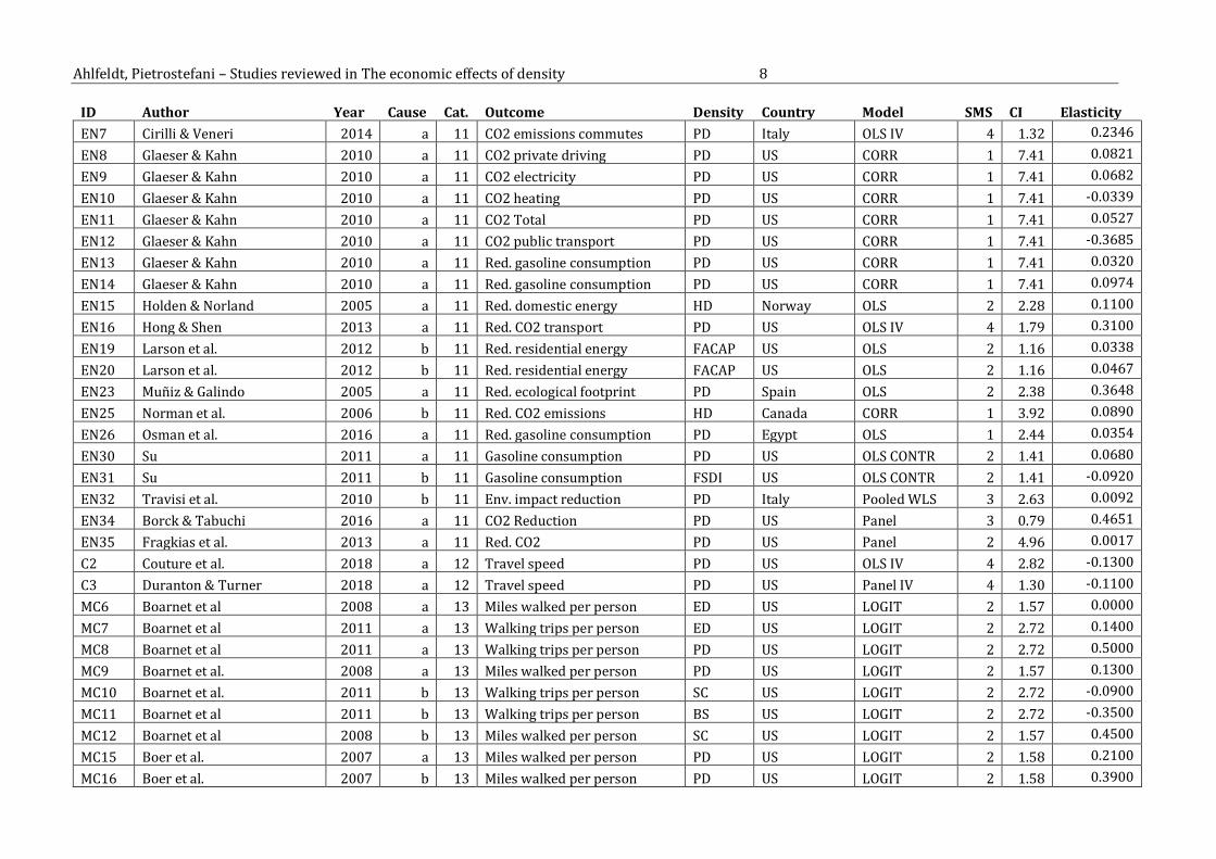
Ahlfeldt, Pietrostefani – Studies reviewed in The economic effects of density 8
ID Author Year Cause Cat. Outcome Density Country Model SMS CI Elasticity
EN7 Cirilli & Veneri 2014 a 11 CO2 emissions commutes PD Italy OLS IV 4 1.32 0.2346
EN8 Glaeser & Kahn 2010 a 11 CO2 private driving PD US CORR 1 7.41 0.0821
EN9 Glaeser & Kahn 2010 a 11 CO2 electricity PD US CORR 1 7.41 0.0682
EN10 Glaeser & Kahn 2010 a 11 CO2 heating PD US CORR 1 7.41 -0.0339
EN11 Glaeser & Kahn 2010 a 11 CO2 Total PD US CORR 1 7.41 0.0527
EN12 Glaeser & Kahn 2010 a 11 CO2 public transport PD US CORR 1 7.41 -0.3685
EN13 Glaeser & Kahn 2010 a 11 Red. gasoline consumption PD US CORR 1 7.41 0.0320
EN14 Glaeser & Kahn 2010 a 11 Red. gasoline consumption PD US CORR 1 7.41 0.0974
EN15 Holden & Norland 2005 a 11 Red. domestic energy HD Norway OLS 2 2.28 0.1100
EN16 Hong & Shen 2013 a 11 Red. CO2 transport PD US OLS IV 4 1.79 0.3100
EN19 Larson et al. 2012 b 11 Red. residential energy FACAP US OLS 2 1.16 0.0338
EN20 Larson et al. 2012 b 11 Red. residential energy FACAP US OLS 2 1.16 0.0467
EN23 Muñiz & Galindo 2005 a 11 Red. ecological footprint PD Spain OLS 2 2.38 0.3648
EN25 Norman et al. 2006 b 11 Red. CO2 emissions HD Canada CORR 1 3.92 0.0890
EN26 Osman et al. 2016 a 11 Red. gasoline consumption PD Egypt OLS 1 2.44 0.0354
EN30 Su 2011 a 11 Gasoline consumption PD US OLS CONTR 2 1.41 0.0680
EN31 Su 2011 b 11 Gasoline consumption FSDI US OLS CONTR 2 1.41 -0.0920
EN32 Travisi et al. 2010 b 11 Env. impact reduction PD Italy Pooled WLS 3 2.63 0.0092
EN34 Borck & Tabuchi 2016 a 11 CO2 Reduction PD US Panel 3 0.79 0.4651
EN35 Fragkias et al. 2013 a 11 Red. CO2 PD US Panel 2 4.96 0.0017
C2 Couture et al. 2018 a 12 Travel speed PD US OLS IV 4 2.82 -0.1300
C3 Duranton & Turner 2018 a 12 Travel speed PD US Panel IV 4 1.30 -0.1100
MC6 Boarnet et al 2008 a 13 Miles walked per person ED US LOGIT 2 1.57 0.0000
MC7 Boarnet et al 2011 a 13 Walking trips per person ED US LOGIT 2 2.72 0.1400
MC8 Boarnet et al 2011 a 13 Walking trips per person PD US LOGIT 2 2.72 0.5000
MC9 Boarnet et al. 2008 a 13 Miles walked per person PD US LOGIT 2 1.57 0.1300
MC10 Boarnet et al. 2011 b 13 Walking trips per person SC US LOGIT 2 2.72 -0.0900
MC11 Boarnet et al 2011 b 13 Walking trips per person BS US LOGIT 2 2.72 -0.3500
MC12 Boarnet et al 2008 b 13 Miles walked per person SC US LOGIT 2 1.57 0.4500
MC15 Boer et al. 2007 a 13 Miles walked per person PD US LOGIT 2 1.58 0.2100
MC16 Boer et al. 2007 b 13 Miles walked per person PD US LOGIT 2 1.58 0.3900
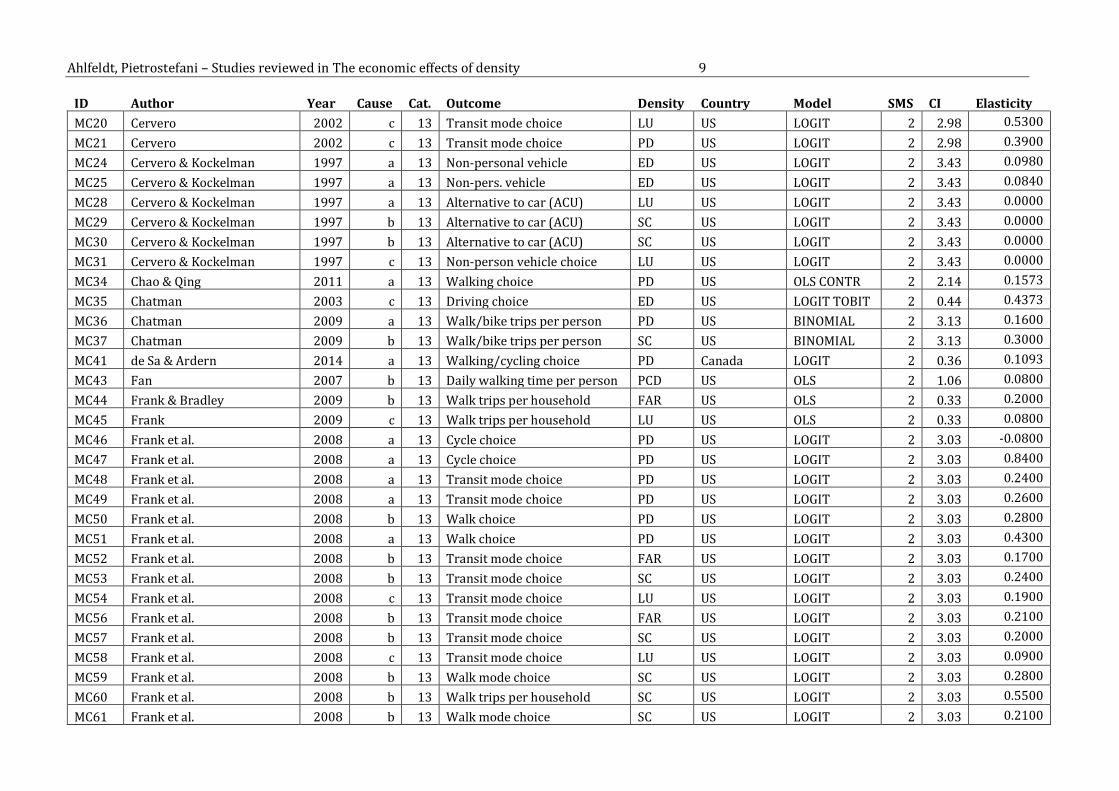
Ahlfeldt, Pietrostefani – Studies reviewed in The economic effects of density 9
ID Author Year Cause Cat. Outcome Density Country Model SMS CI Elasticity
MC20 Cervero 2002 c 13 Transit mode choice LU US LOGIT 2 2.98 0.5300
MC21 Cervero 2002 c 13 Transit mode choice PD US LOGIT 2 2.98 0.3900
MC24 Cervero & Kockelman 1997 a 13 Non-personal vehicle ED US LOGIT 2 3.43 0.0980
MC25 Cervero & Kockelman 1997 a 13 Non-pers. vehicle ED US LOGIT 2 3.43 0.0840
MC28 Cervero & Kockelman 1997 a 13 Alternative to car (ACU) LU US LOGIT 2 3.43 0.0000
MC29 Cervero & Kockelman 1997 b 13 Alternative to car (ACU) SC US LOGIT 2 3.43 0.0000
MC30 Cervero & Kockelman 1997 b 13 Alternative to car (ACU) SC US LOGIT 2 3.43 0.0000
MC31 Cervero & Kockelman 1997 c 13 Non-person vehicle choice LU US LOGIT 2 3.43 0.0000
MC34 Chao & Qing 2011 a 13 Walking choice PD US OLS CONTR 2 2.14 0.1573
MC35 Chatman 2003 c 13 Driving choice ED US LOGIT TOBIT 2 0.44 0.4373
MC36 Chatman 2009 a 13 Walk/bike trips per person PD US BINOMIAL 2 3.13 0.1600
MC37 Chatman 2009 b 13 Walk/bike trips per person SC US BINOMIAL 2 3.13 0.3000
MC41 de Sa & Ardern 2014 a 13 Walking/cycling choice PD Canada LOGIT 2 0.36 0.1093
MC43 Fan 2007 b 13 Daily walking time per person PCD US OLS 2 1.06 0.0800
MC44 Frank & Bradley 2009 b 13 Walk trips per household FAR US OLS 2 0.33 0.2000
MC45 Frank 2009 c 13 Walk trips per household LU US OLS 2 0.33 0.0800
MC46 Frank et al. 2008 a 13 Cycle choice PD US LOGIT 2 3.03 -0.0800
MC47 Frank et al. 2008 a 13 Cycle choice PD US LOGIT 2 3.03 0.8400
MC48 Frank et al. 2008 a 13 Transit mode choice PD US LOGIT 2 3.03 0.2400
MC49 Frank et al. 2008 a 13 Transit mode choice PD US LOGIT 2 3.03 0.2600
MC50 Frank et al. 2008 b 13 Walk choice PD US LOGIT 2 3.03 0.2800
MC51 Frank et al. 2008 a 13 Walk choice PD US LOGIT 2 3.03 0.4300
MC52 Frank et al. 2008 b 13 Transit mode choice FAR US LOGIT 2 3.03 0.1700
MC53 Frank et al. 2008 b 13 Transit mode choice SC US LOGIT 2 3.03 0.2400
MC54 Frank et al. 2008 c 13 Transit mode choice LU US LOGIT 2 3.03 0.1900
MC56 Frank et al. 2008 b 13 Transit mode choice FAR US LOGIT 2 3.03 0.2100
MC57 Frank et al. 2008 b 13 Transit mode choice SC US LOGIT 2 3.03 0.2000
MC58 Frank et al. 2008 c 13 Transit mode choice LU US LOGIT 2 3.03 0.0900
MC59 Frank et al. 2008 b 13 Walk mode choice SC US LOGIT 2 3.03 0.2800
MC60 Frank et al. 2008 b 13 Walk trips per household SC US LOGIT 2 3.03 0.5500
MC61 Frank et al. 2008 b 13 Walk mode choice SC US LOGIT 2 3.03 0.2100

Ahlfeldt, Pietrostefani – Studies reviewed in The economic effects of density 10
ID Author Year Cause Cat. Outcome Density Country Model SMS CI Elasticity
MC63 Greenwald & Boarnet 2001 a 13 Walk trips per person PD US PROBIT 2 0.07 0.3400
MC64 Joh et al. 2009 a 13 Walk trips per person ED US OLS 2 0.34 0.1900
MC65 Joh et al 2009 b 13 Walk trips per person SC US OLS 2 0.34 -0.2700
MC66 Joh et al 2009 b 13 Walk trips per person BS US OLS 2 0.34 0.0100
MC68 Cervero & Kockelman 1997 a 13 Walk/bike mode choice ED US OLS 2 0.87 0.0000
MC69 Cervero & Kockelman 1997 a 13 Walk/bike mode choice PD US OLS 2 0.87 0.0000
MC70 Cervero & Kockelman 1997 c 13 Walk/bike mode choice LU US OLS 2 0.87 0.2300
MC73 Lund et al. 2004 b 13 Transit mode choice SC US LOGIT 2 1.14 1.0800
MC79 Nielsen et al. 2013 a 13 Cycle distance PD Denmark Heckman 4 1.86 0.0870
MC81 Pouyanne 2004 a 13 Car share rate PD France OLS, LOGIT 2 0.34 -0.0210
MC82 Pouyanne 2004 a 13 Cycling choice PD France OLS, LOGIT 2 0.34 2.0143
MC83 Pouyanne 2004 a 13 Public transport choice PD France OLS, LOGIT 2 0.34 0.4203
MC84 Pouyanne 2004 a 13 Walking choice PD France OLS, LOGIT 2 0.34 0.4390
MC85 Rajamani & Handy 2003 c 13 Transit mode choice LU US LOGIT 2 1.04 -0.0400
MC86 Rajamani et al 2003 a 13 Walk mode choice PD US LOGIT 2 1.04 0.0100
MC87 Rajamani et al 2003 c 13 Walk mode choice LU US LOGIT 2 1.04 0.3600
MC88 Reilly & Landis 2002 a 13 Transit mode choice PD US LOGIT 2 0.36 0.2000
MC89 Reilly 2002 a 13 Walk mode choice PD US LOGIT 2 0.36 0.1600
MC90 Rodríguez & Joo 2004 a 13 Transit mode choice PD US LOGIT 2 2.80 -0.2000
MC93 Targa et al. 2005 a 13 Walk trips per person PD US Poisson 2 0.35 0.0300
MC94 Targa & Clifton 2005 b 13 Walk trips per person BS US Poisson 2 0.35 0.3200
MC95 Targa & Clifton 2005 c 13 Walk trips per person LU US Poisson 2 0.35 0.0800
MC98 Zegras 2007 b 13 Daily automobile use BD Chile OLS -LOGIT 2 0.89 -0.0400
MC99 Zegras 2007 b 13 Automobile use per household SC Chile OLS -LOGIT 2 0.89 -0.1500
MC100 Zegras 2007 c 13 Automobile use per household LU Chile OLS -LOGIT 2 0.89 -0.0100
MC101 Zhang 2004 a 13 Driving choice red. ED Hong Kong LOGIT 2 1.63 0.0700
MC102 Zhang 2004 a 13 Driving choice red. PD Hong Kong LOGIT 2 1.63 0.1100
MC103 Zhang 2004 a 13 Driving choice ED Hong Kong LOGIT 2 1.63 0.0770
MC104 Zhang 2004 a 13 Driving choice PD Hong Kong LOGIT 2 1.63 0.0390
MC105 Zhang 2004 a 13 Taxi red. ED Hong Kong LOGIT 2 1.63 0.0240
MC106 Zhang 2004 a 13 Taxi red. PD Hong Kong LOGIT 2 1.63 0.1280

Ahlfeldt, Pietrostefani – Studies reviewed in The economic effects of density 11
ID Author Year Cause Cat. Outcome Density Country Model SMS CI Elasticity
MC107 Zhang 2004 a 13 Taxi red. ED Hong Kong LOGIT 2 1.63 0.1180
MC108 Zhang 2004 a 13 Taxi red. PD Hong Kong LOGIT 2 1.63 0.0260
MC109 Zhang 2004 a 13 Public transport choice ED Hong Kong LOGIT 2 1.63 0.0060
MC110 Zhang 2004 a 13 Public transport choice PD Hong Kong LOGIT 2 1.63 0.0140
MC111 Zhang 2004 a 13 Transit choice ED Hong Kong LOGIT 2 1.63 0.0110
MC112 Zhang 2004 a 13 Transit choice PD Hong Kong LOGIT 2 1.63 0.0050
MC113 Zhang 2004 a 13 Driving choice red. ED US LOGIT 2 1.63 0.0010
MC114 Zhang 2004 a 13 Driving choice red. PD US LOGIT 2 1.63 0.0400
MC115 Zhang 2004 a 13 Car share red. ED US LOGIT 2 1.63 0.0030
MC116 Zhang 2004 a 13 Car share red. PD US LOGIT 2 1.63 0.0330
MC117 Zhang 2004 a 13 Car share red. ED US LOGIT 2 1.63 0.0440
MC118 Zhang 2004 a 13 Car share PD US LOGIT 2 1.63 0.0710
MC119 Zhang 2004 a 13 Driving choice ED US LOGIT 2 1.63 0.0310
MC120 Zhang 2004 a 13 Driving choice PD US LOGIT 2 1.63 0.0440
MC121 Zhang 2004 a 13 Public transport choice ED US LOGIT 2 1.63 0.0040
MC122 Zhang 2004 a 13 Public transport choice PD US LOGIT 2 1.63 0.1260
MC123 Zhang 2004 a 13 Transit choice ED US LOGIT 2 1.63 0.0900
MC124 Zhang 2004 a 13 Transit choice PD US LOGIT 2 1.63 0.1180
MC125 Zhang 2004 a 13 Walking/cycling choice ED US LOGIT 2 1.63 0.0040
MC126 Zhang 2004 a 13 Walking/cycling choice PD US LOGIT 2 1.63 0.0600
MC127 Zhang 2004 a 13 Walking/cycling ED US LOGIT 2 1.63 0.0260
MC128 Zhang 2004 a 13 Walk choice PD US LOGIT 2 1.63 0.1050
MC129 Zhao 2014 a 13 Cycling choice ED China LOGIT 2 2.78 0.1265
MC130 Zhao 2014 a 13 Cycling choice PD China LOGIT 2 2.78 0.0034
MC133 Zhao 2014 a 13 Walking choice ED China LOGIT 2 2.78 0.0418
MC134 Zhao 2014 a 13 Walking choice PD China LOGIT 2 2.78 0.0013
MC135 Cervero & Kockelman 1997 a 13 Non-pers. vehicle ED US LOGIT 2 3.43 0.1130
H1 Chaix et al. 2006 a 14 IHD risk red. PD Sweden Panel LOGIT 3 2.40 -0.2986
H2 Chaix et al. 2006 a 14 Lung cancer risk red. PD Sweden Panel LOGIT 3 2.40 -0.1949
H3 Chaix et al. 2006 a 14 Pulmonary disease red. PD Sweden Panel LOGIT 3 2.40 -0.5779
H4 Fecht et al. 2016 a 14 Premature mortalities PD UK CrossSec 2 2.40 -0.2900

Ahlfeldt, Pietrostefani – Studies reviewed in The economic effects of density 12
ID Author Year Cause Cat. Outcome Density Country Model SMS CI Elasticity
H5 Fecht et al. 2016 b 14 Premature mortalities SDI UK CrossSec 2 1.22 -0.5000
H6 Graham & Glaister 2003 a 14 KSI reduction ED UK LOGLIN 2 0.88 -0.0510
H7 Graham & Glaister 2003 a 14 KSI reduction PD UK LOGLIN 2 0.88 0.3990
H9 Graham & Glaister 2003 a 14 Pedestrian casualty red. ED UK LOGLIN 2 0.88 -0.8260
H10 Graham & Glaister 2003 a 14 Pedestrian casualty red. PD UK LOGLIN 2 0.88 0.5290
H12 Howe et al. 1993 a 14 Red. all cancer rate PD US COR 1 0.51 -0.0550
H14 Mahoney et al. 1990 a 14 Mortality red. (all cancers) PD US LOGIT 2 2.55 -0.0380
H15 Melis et al. 2015 a 14 Red. metal health prescript. PD Italy OLS, panel 2 1.54 0.0127
H16 Reijneveld et al. 1999 a 14 Mortality red. PD Netherlands LOGLIN 2 0.29 -0.0906
WB3 Brueckner & Largey 2006 a 15 # times attends club meeting PD US PROBIT IV 4 1.10 -0.0796
WB4 Brueckner & Largey 2006 a 15 # people can confide in PD US PROBIT IV 4 1.10 -0.0056
WB5 Brueckner & Largey 2006 a 15 # close friends PD US PROBIT IV 4 1.10 -0.0081
WB6 Brueckner & Largey 2006 a 15 Social contacts PD US PROBIT IV 4 1.10 -0.0159
WB7 Brueckner & Largey 2006 a 15 Visit neighbour/week PD US PROBIT IV 4 1.10 -0.0446
WB8 Fassio et al. 2013 a 15 Self-rep. env. health PD Italy COR 1 1.97 -0.3384
WB9 Fassio et al. 2013 a 15 Self-rep. social satisfaction PD Italy COR 1 1.97 -0.4232
WB10 Fassio et al. 2013 a 15 Self-rep. physical health PD Italy COR 1 1.97 -0.1380
WB11 Fassio et al. 2013 a 15 Self-rep. psychological status PD Italy COR 1 1.97 -0.3189
WB12 Glaeser et al. 2016 a 15 Self-rep. well-being PD US Panel 3 1.30 -0.0037
WB13 Harvey et al. 2015 b 15 Perceived safety FAR US OLS, LOGIT 2 1.07 0.0690
WB10 Fassio et al. 2013 a 15 Self-rep. physical health PD Italy COR 1 1.96 -0.1380

Ahlfeldt, Pietrostefani – Studies reviewed in The economic effects of density 13
Legend
Cause CI Maryland Scientific Method Scale
(WWC)
a Residential and employment density Citations Index 0 Descriptive data
b Morphological density 1 Correlations, cross-sectional no control variables
c Mixed Use 2 Cross-sectional, adequate control variables
Category Density 3 Panel data methods 1 Productivity PD Population density 4 Instrumental variables, RDD 2 Innovation
ED Employment or other economic density 5 Randomised control trials
3 Value of space SPP Spillover potential 4 Job accessibility HD Development density 5 Services access FACAP Floor area per capita 6 Efficiency of public services delivery GAR Geographic area reduction 7 Social equity
FAR Floor area ration and related measures
8 Safety FSDI Freeway density 9 Open space preservation and biodiversity
10 Pollution reduction 11 Energy efficiency 12 Traffic flow 13 Sustainable mode choice 14 Health 15 Wellbeing

Ahlfeldt, Pietrostefani – Studies reviewed in The economic effects of density 14
Full Bibliography
Abel, J.R., Dey, I. & Gabe, T.M., 2012. Productivity and the density of Human Capital. Journal of Regional Science, 52(4), pp.562–586.
Aberg, Y., 1973. Regional Productivity Differences in Swedish Manufacturing. Regional and Urban Economics, 3(2). Ahlfeldt, G.M., Redding, S.J., et al., 2015. The Economics of Density: Evidence from the Berlin Wall. Econometrica, 83(6),
pp.2127–2189. Ahlfeldt, G.M. & Feddersen, A., 2015. From Periphery to Core : Measuring Agglomeration Effects Using High-Speed Rail. Working
Paper. Ahlfeldt, G.M. & Maennig, W., 2015. Homevoters vs. leasevoters: A spatial analysis of airport effects. Journal of Urban
Economics, 87. Ahlfeldt, G.M., Moeller, K. & Wendland, N., 2015. Chicken or egg? The PVAR econometrics of transportation. Journal of
Economic Geography, 15(6), pp.1169–1193. Ahlfeldt, G.M. & Wendland, N., 2013. How polycentric is a monocentric city ? Centers, spillovers and hysteresis. Journal of
Economic Geography, 13(September 2012), pp.53–83. Albouy, D., 2008. Are Big Cities Bad Places to Live? Estimating Quality of Life across Metropolitan Areas. National Bureau of
Economic Research Working Paper 14472. Albouy, D. & Lue, B., 2015. Driving to opportunity: Local rents, wages, commuting, and sub-metropolitan quality of life. Journal
of Urban Economics, 89, pp.74–92. Albouy, D. & Stuart, B., 2014. Urban Population and Amenities. National Bureau of Economic Research, Inc. NBER Working
Papers: 19919. Ananat, E., Fu, S. & Ross, S.L., 2013. Race-Specific Agglomeration Economies: Social Distance and the Black-White Wage Gap.
NBER Working Paper 18933 (National Bureau of Economic Research), pp.13–24. Andersson, M., Klaesson, J. & Larsson, J.P., 2016. How Local are Spatial Density Externalities? Neighbourhood Effects in
Agglomeration Economies. Regional Studies, 50(6), pp.1082–1095. Andersson, M., Klaesson, J. & Larsson, J.P., 2014. The sources of the urban wage premium by worker skills : Spatial sorting or
agglomeration economies ? Papers in Regional Science, 93(4), pp.727–747. Andersson, R., Quigley, J.M. & Wilhelmsson, M., 2005. Agglomeration and the spatial distribution of creativity. Papers in
Regional Science, 84(3), pp.445–464. Au, C.-C. & Henderson, J.V., 2006. Are Chinese cities really too small? Review of Economic Studies, 73, pp.549–576. Baldwin, J.R. et al., 2007. Urban Economies and Productivity, Baldwin, J.R., Brown, W.M. & Rigby, D.L., 2010. Agglomeration economies: Microdata panel estimates from Canadian
manufacturing. Journal of Regional Science, 50(5), pp.915–934. Barde, S., 2010. Increasing Returns and the Spatial Structure of French Wages. Spatial Economic Analysis, 5(1), p.73. Barter, P.A., 2000. Transport Dilemmas in Dense Urban Areas: Examples from Eastern Asia. In Compact Cities: Sustainable Urban
Forms for Developing Countries. London & New York: SPON Press. Barufi, A.M.B., Haddad, E.A. & Nijkamp, P., 2016. Industrial scope of agglomeration economies in Brazil. Annals of Regional
Science, 56(3), pp.707–755. Baum-Snow, N., Freedman, M. & Pavan, R., 2016. Why Has Urban Inequality Increased ? Baum-Snow, N. & Pavan, R., 2012a. Understanding the city size wage gap. Review of Economic Studies, 79(1), pp.88–127. Baum-Snow, N. & Pavan, R., 2012b. Understanding the City Size Wage Gap. Review Econ Stud, 79(1), pp.247–253. Bento, A. et al., 2005. The Effects of Urban Spatial Structure on Travel Demand in the United States. Review of Economics and
Statistics, 87(3), pp.466–478. Bettencourt, L.M.A., Lobo, J. & Strumsky, D., 2007. Invention in the city: Increasing returns to patenting as a scaling function of
metropolitan size. Research Policy, 36(1), pp.107–120. Bhat, C.R., Sen, S. & Eluru, N., 2009. The impact of demographics, built environment attributes, vehicle characteristics, and
gasoline prices on household vehicle holdings and use. Transportation Research B. Boarnet, M. et al., 2011. Retrofitting the suburbs to increase walking: Evidence from a land-use-travel study. Urban Studies,
48(1), pp.129–159. Boarnet, M.G., Greenwald, M. & McMillan, T.E., 2008. Walking, urban design, and health: Toward a cost-benefit analysis
framework. Journal of Planning Education and Research, 27(3), pp.341–358. Boer, R. et al., 2007. Neighborhood Design and Walking Trips in Ten U.S. Metropolitan Areas. Am J Prev Med, 32(4), pp.298–304. Borck, R. & Schrauth, P., 2018. Population density and (urban) air quality. Preliminary and Incomplete Working Paper. Borck, R. & Tabuchi, T., 2016. Pollution and City Size: Can Cities be Too Small ? RIETI Discussion Paper Series 16-E-094 University
of Potsdam. Brownstone, D. & Thomas, F.G., 2013. The impact of residential density on vehicle usage and fuel consumption: Evidence from
national samples. Energy Economics, 40(1), pp.196–206. Brueckner, J.K. & Largey, A.G., 2006. Social interaction and urban sprawl. CESifo WP, 1843(1), pp.18–34.

Ahlfeldt, Pietrostefani – Studies reviewed in The economic effects of density 15 Brülhart, M. & Mathys, N.A., 2008. Sectoral agglomeration economies in a panel of European regions. Regional Science and
Urban Economics, 38(4), pp.348–362. Carlino, G.A., Chatterjee, S. & Hunt, R.M., 2007. Urban density and the rate of invention. Journal of Urban Economics, 61(3),
pp.389–419. Carozzi, F. & Roth, S., 2018. Dirty Density : Air Quality and the Denisty of American Cities. Preliminary and Incomplete Working
Paper. Carruthers, J.I. & Ulfarsson, G.F., 2003. Urban sprawl and the cost of public services. Environment and Planning B: Planning and
Design, 30(4), pp.503–522. Cervero, R., 2002. Built environments and mode choice: Toward a normative framework. Transportation Research Part D:
Transport and Environment, 7(4), pp.265–284. Cervero, R. & Kockelman, K., 1997. Travel demand and the 3Ds: Density, diversity, and design. Transportation Research Part D:
Transport and Environment, 2(3), pp.199–219. Chaix, B. et al., 2006. Disentangling contextual effects on cause-specific mortality in a longitudinal 23-year follow-up study:
Impact of population density or socioeconomic environment? International Journal of Epidemiology, 35(3), pp.633–643. Champman, J., Frank, L. & Georgia, G.D. of T. and S. of, 2004. Integrating Travel Behavior and Urban Form Data to Address
Transportation and Air Quality Problems in Atlanta. Smartraq, p.304. Chao, L. & Qing, S., 2011. An empirical analysis of the influence of urban form on household travel and energy consumption.
Computers, Environment and Urban Systems, 35(5), pp.347–357. Chatman, D., 2003. How Density and Mixed Uses at the Workplace Affect Personal Commercial Travel and Commute Mode
Choice. Transportation Research Record, 1831(03), pp.193–201. Chatman, D.G., 2008. Deconstructing development density: Quality, quantity and price effects on household non-work travel.
Transportation Research Part A: Policy and Practice, 42(7), pp.1008–1030. Chauvin, J.P. et al., 2016. What is different about urbanization in rich and poor countries? Cities in Brazil, China, India and the
United States. Journal of Urban Economics, pp.1–33. Cheshire, P.C. & Dericks, G.H., 2018. “Trophy architects” as deadweight loss: rent acquisition by design in the constrained
London office market. Working Paper. Ciccone, A., 2002. Agglomeration effects in Europe. European Economic Review, 46(2), pp.213–227. Ciccone, A. & Hall, R.E., 1996. Productivity and the Density of Economic Activity Productivity and the Density of Economic
Activity. The American Economic Review, 86(1), pp.54–70. Cingano, F. & Schivardi, F., 2004. Identifying the Sources of Local. Journal of the European Economic Association, 2(June),
pp.720–742. Cirilli, A. & Veneri, P., 2014. Spatial Structure and Carbon Dioxide (CO2 ) Emissions Due to Commuting: An Analysis of Italian
Urban Areas. Regional Studies, 48(12), pp.1993–2005. Combes, P.-P. et al., 2012. The Productivity Advantages of Large Cities: Distinguishing Agglomeration From Firm Selection.
Econometrica, 80(6), pp.2543–2594. Combes, P.-P., Démurger, S. & Li, S., 2017. Productivity gains from agglomeration and migration in Chinese cities over 2002-
2013. Asian Development Review, 34(2), pp.184–200. Combes, P.-P., Duranton, G. & Gobillon, L., 2008. Spatial wage disparities: Sorting matters! Journal of Urban Economics, 63(2),
pp.723–742. Combes, P., Duranton, G. & Gobillon, L., 2018. The Costs of Agglomeration: Land Prices in French Cities. The Review of Economic
Studies, (7027). Combes, P. & Li, S., 2018. Unequal Migration and Urbanisation Gains in China 1. Combes, P.P., Démurger, S. & Li, S., 2015. Migration externalities in Chinese cities. European Economic Review, 76, pp.152–167. Couture, V., 2016. Valuing the Consumption Benefits of Urban Density. Working Paper: Univeristy of California, Berkeley,
(September). Couture, V., Duranton, G. & Turner, M.A., 2018. Speed. The Review of Economics and Statistics, 100(4), pp.735–739. Davis, D.R. & Weinstein, D.E., 2001. Market size, linkages, and productiviy: a study of japanese regions. Geography, pp.1–29. Dekle, R. & Eaton, J., 1999. Agglomeration and Land Rents: Evidence from the Prefectures. Journal of Urban Economics, 46(2),
pp.200–214. Dericks, G.H. & Koster, H.R.A., 2018. The Billion Pound Drop : The Blitz and Agglomeration Economics in London. CEP Discussion
Paper No 1542, (1542). Duranton, G. & Turner, M.A., 2018. Urban form and driving: Evidence from US cities. Journal of Urban Economics, 108, pp.170–
191. Echeverri-Carroll, E.L. & Ayala, S.G., 2011. Urban Wages : Does City Size Matter ? Urban Studies, 48(2), pp.253–271. Eckert, F., Hejlesen, M. & Walsh, C., 2018. The Return to Big City Experience : Evidence from Danish. Working Paper. Faberman, R.J. & Freedman, M., 2016. The urban density premium across establishments. Journal of Urban Economics, 93,
pp.71–84. Fan, Y., 2007. The built environment, activity space, and time allocation: An activity-based framework for modeling the land use
and travel connection. , p.189. Fassio, O., Rollero, C. & De Piccoli, N., 2013. Health, Quality of Life and Population Density: A Preliminary Study on
“Contextualized” Quality of Life. Social Indicators Research, 110(2), pp.479–488.
Ahlfeldt, Pietrostefani – Studies reviewed in The economic effects of density 16 Fecht, D. et al., 2016. Associations between urban metrics and mortality rates in England. Environmental health : a global access
science source, 15 Suppl 1(Suppl 1), p.34. Fingleton, B., 2003. Increasing returns: evidence from local wage rates in Great Britain. Oxford Economic Papers, 55(4), pp.716–
739. Fingleton, B., 2006. The new economic geography versus urban economics: An evaluation using local wage rates in Great Britain.
Oxford Economic Papers, 58(3), pp.501–530. Fragkias, M. et al., 2013. Does Size Matter? Scaling of CO2 Emissions and U.S. Urban Areas. PLoS ONE, 8(6). Frank, L. et al., 2008. Urban form, travel time, and cost relationships with tour complexity and mode choice. Transportation,
35(1), pp.37–54. Frank, L. & Bradley, M., 2009. I-PLACE3S Health & Climate Enhancements and Their Application in King County. REPORT, pp.1–
59. Fu, S., 2007. Smart Café Cities: Testing human capital externalities in the Boston metropolitan area. Journal of Urban Economics,
61(1), pp.86–111. Galster, G. & Cutsinger, J., 2007. Racial Settlement and Metropolitan Land-Use Patterns: Does Sprawl Abet Black-White
segregation? Urban Geography, 28(6), pp.516–553. Glaeser, E.L., Gottlieb, J.D. & Ziv, O., 2016. Unhappy Cities. Journal of Labor Economics, 34(2), pp.S129–S182. Glaeser, E.L. & Kahn, M.E., 2010. The greenness of cities: Carbon dioxide emissions and urban development. Journal of Urban
Economics, 67(3), pp.404–418. Glaeser, E.L. & Sacerdote, B., 1999. Why is There More Crime in Cities ? Journal of Political Economy, 107(No. S6 December
1999), pp.S225–S258. Graham, D.J., 2007a. Agglomeration, productivity and transport investment. Journal of Transport Economics and Policy, 41(3),
pp.317–343. Graham, D.J., 2000. Spatial variation in labour productivity in British manufacturing. International Review of Applied Economics,
14(3), pp.323–341. Graham, D.J. et al., 2010. Testing for causality between productivity and agglomeration economies. Journal of Regional Science,
50(5), pp.935–951. Graham, D.J., 2007b. Variable returns to agglomeration and the effect of road traffic congestion. Journal of Urban Economics,
62(1), pp.103–120. Graham, D.J. & Glaister, S., 2003. Spatial Variation in Road Pedestrian Casualties: The Role of Urban Scale, Density and Land-use
Mix. Urban Studies, 40(8), pp.1591–1607. Graham, D.J. & Kim, H.Y., 2008. An empirical analytical framework for agglomeration economies. Annals of Regional Science,
42(2), pp.267–289. Greenwald, M. & Boarnet, M., 2001. Built Environment as Determinant of Walking Behavior: Analyzing Nonwork Pedestrian
Travel in Portland, Oregon. Transportation Research Record: Journal of the Transportation Research Board, 1780, pp.33–41.
Harvey, C. et al., 2015. Effects of skeletal streetscape design on perceived safety. Landscape and Urban Planning, 142, pp.18–28. Henderson, J.V., 1986. Efficiency of resource usage and city size. Journal of Urban Economics, 19(1), pp.47–70. Henderson, J.V., 2003. Marshall’s scale economies. Journal of Urban Economics, 53(1), pp.1–28. Hilber, C. & Palmer, C., 2014. Urban Development and Air Pollution: Evidence from a Global Panel of Cities. SSRN Electronic
Journal, (175). Holden, E. & Norland, I., 2005. Three challenges for the compact city as a sustainable urban form: Household consumption of
energy and transport in eight residential areas in the greater Oslo Region. Urban Studies, 42(12), pp.2145–2166. Holtzclaw, J. et al., 2002. Location efficiency: Neighborhood and socio-economic characteristics determine auto ownership and
use - Studies in Chicago, Los Angeles and San Francisco. Transportation Planning and Technology, 25(1), pp.1–27. Hong, J. & Shen, Q., 2013. Residential density and transportation emissions : Examining the connection by addressing spatial
autocorrelation and self-selection. Transportation Research Part D, 22, pp.75–79. Hortas-Rico, M. & Sole-Olle, A., 2010. Does Urban Sprawl Increase the Costs of Providing Local Public Services? Evidence from
Spanish Municipalities. Urban Studies, 47(7), pp.1513–1540. Howe, H.L., Keller, J.E. & Lehnherr, M., 1993. Relation between Population Density and Cancer Incidence, Illinois, 1986-1990.
American Journal of Epidemiology, 138(1), pp.29–36. Joh, K., Boarnet, M.G. & Nguyen, M.T., 2009. Interactions between race/ethnicity, attitude, and crime: Analyzing walking trips in
the South Bay Area. Paper presented at the 88th annual meeting of the Transportation Research Board, Washington, DC. In Washington, DC: Paper presented at the 88th annual meeting of the Transportation Research Board.
Kanemoto, Y., Ohkawara, T. & Suzuki, T., 1996. Agglomeration economies and a test for optimal city sizes in Japan. Journal of the
Japanese and International Economies, 10(4), pp.379–398. Kholodilin, K.A. & Ulbricht, D., 2015. Urban house prices: A tale of 48 cities. Economics, 9. Knudsen, B. et al., 2008. Density and creativity in U.S. Regions. Annals of the Association of American Geographers, 98(2),
pp.461–478. Koster, H., van Ommeren, J.N. & Rietveld, P., 2014. Agglomeration Economies and Productivity: A Structural Estimation
Approach Using Commercial Rents. Economica, 81, pp.63–85. Ladd, H.F., 1994. Fiscal impacts of local population growth: A conceptual and empirical analysis. Regional Science and Urban

Ahlfeldt, Pietrostefani – Studies reviewed in The economic effects of density 17 Economics, 24(6), pp.661–686.
Lall, S. V., Shalizi, Z. & Deichmann, U., 2004. Agglomeration economies and productivity in Indian industry. Journal of
Development Economics, 73(2), pp.643–673. Larson, W., Liu, F. & Yezer, A., 2012. Energy footprint of the city: Effects of urban land use and transportation policies. Journal of
Urban Economics, 72(2–3), pp.147–159. Larsson, J.P., 2014. The neighborhood or the region? Reassessing the density-wage relationship using geocoded data. Annals of
Regional Science, 52(2), pp.367–384. Levinson, D., 2008. Density and dispersion: The co-development of land use and rail in London. Journal of Economic Geography,
8(1), pp.55–77. Lin, B., Meyers, J. & Barnett, G., 2015. Understanding the potential loss and inequities of green space distribution with urban
densification. Urban Forestry and Urban Greening, 14(4), pp.952–958. Liu, C.H., Rosenthal, S.S. & Strange, W.C., 2016. The Vertical City: Rent Gradients and Spatial Structure, Lund, H., Cervero, R. & Willson, R., 2004. Travel characteristics of transit-oriented development in California. Sacramento, CA:
California Department of …, 5313(January). Lynch, A.K. & Rasmussen, D.W., 2004. Proximity, Neighbourhood and the Efficacy of Exclusion. Urban Studies, 41(2), pp.285–98. Mahoney, M.C. et al., 1990. Population density and cancer incidence differentials in New York State, 1978-82. International
Journal of Epidemiology, 19(3), pp.483–490. Melis, G. et al., 2015. The effects of the urban built environment on mental health: A cohort study in a large northern Italian city.
International Journal of Environmental Research and Public Health, 12(11), pp.14898–14915. Mion, G. & Naticchioni, P., 2005. Urbanization externalities, market potential and spatial sorting of skills and firms. , (February),
pp.1–45. Monkkonen, P. et al., 2018. Are Workers More Productive in More Compact Cities? Evidence from Mexico. Working Paper. Moomaw, R.L., 1985. Firm location and city size: Reduced productivity advantages as a factor in the decline of manufacturing in
urban areas. Journal of Urban Economics, 17(1), pp.73–89. Moomaw, R.L., 1983. Is population scale a worthless surrogate for business agglomeration economies? Regional Science and
Urban Economics, 13(4), pp.525–545. Morikawa, M., 2011. Economies of Density and Productivity in Service Industries: An Analysis of Personal Service Industries
Based on Establishment-Level Data. Review of Economics and Statistics, 93(1), pp.179–192. Muñiz, I. & Galindo, A., 2005. Urban form and the ecological footprint of commuting. The case of Barcelona. Ecological
Economics, 55(4), pp.499–514. Nakamura, R., 1985. Agglomeration economies in urban manufacturing industries: A case of Japanese cities. Journal of Urban
Economics, 17(1), pp.108–124. Nielsen, T.A.S. et al., 2013. Environmental correlates of cycling: Evaluating urban form and location effects based on Danish
micro-data. Transportation Research Part D: Transport and Environment, 22, p.4044. Norman, J., MacLean, H. & Kennedy, C., 2006. Comparing high and low residential density: life-cycle analysis of energy use and
greenhouse gas emissions. J Urban Plann Dev, 132(1), pp.10–21. Ó hUallacháin, B., 1999. Patent Places: Size Matters. Journal of Regional Science, 39(4), pp.613–636. Osman, T., Divigalpitiya, P. & Osman, M.M., 2016. The impact of Built Environment Characteristics on Metropolitans Energy
Consumption: An Example of Greater Cairo Metropolitan Region. Buildings, 6(2), p.12. Palm, M. et al., 2014. The trade-offs between population density and households’ transportation-housing costs. Transport
Policy, 36, pp.160–172. Pickrell, D.O.N. & Schimek, P., 1997. Growth in Motor Vehicle Ownership and Use : , pp.1–17. Pouyanne, G., 2004. Urban Form and Travel Patterns. Working Paper, pp.1–39. Prieto, Á.M., Zofío, J.L. & Álvarez, I., 2015. Cost economies, urban patterns and population density: The case of public
infrastructure for basic utilities. Papers in Regional Science, 94(4), pp.795–816. Rajamani, J. & Handy, S., 2003. Assessing the impact of urban form measures on nonwork trip mode choice after controlling for
demographic and level-of-service effects. Working Paper, (301). Raleigh, E. & Galster, G., 2015. Neighborhood Disinvestment, Abandonment, And Crime Dynamics. Journal of Urban Affairs,
37(4), pp.367–396. Rappaport, J., 2008. A productivity model of city crowdedness. Journal of Urban Economics, 63(2), pp.715–722. Reijneveld, S.A., Verheij, R.A. & de Bakker, D.H., 1999. Relative importance of urbanicity, ethnicity and socioeconomic factors
regarding area mortality differences. Journal of epidemiology and community health, 53(7), pp.444–5. Reilly, M. & Landis, J., 2002. The Influence of Built-Form and Land Use on Mode Choice. Working Paper, pp.1–51. Rice, P., Venables, A.J. & Patacchini, E., 2006. Spatial determinants of productivity: Analysis for the regions of Great Britain.
Regional Science and Urban Economics, 36(6), pp.727–752. Rodríguez, D.A. & Joo, J., 2004. The relationship between non-motorized mode choice and the local physical environment.
Transportation Research Part D: Transport and Environment, 9(2), pp.151–173. Rosenthal, S.S. & Strange, W.C., 2008. The attenuation of human capital spillovers. Journal of Urban Economics, 64(2), pp.373–
389. Rothwell, J. & Massey, D.S., 2009. The Effect of Density Zoning on Racial Segregation in U.S. Urban Areas. Urban Affairs Review,
44(6), pp.779–806.

Ahlfeldt, Pietrostefani – Studies reviewed in The economic effects of density 18 Rothwell, J.T., 2011. Racial enclaves and density zoning: The institutionalized segregation of racial minorities in the United
States. American Law and Economics Review, 13(1), pp.290–358. Rothwell, J.T. & Massey, D.S., 2010. Density zoning and class segregation in U.S. metropolitan areas. Social Science Quarterly,
91(5), pp.1123–1143. de Sa, E. & Ardern, C.I., 2014. Associations between the built environment, total, recreational, and transit-related physical
activity. BMC public health, 14(1), p.693. Salomons, E.M. & Berghauser Pont, M., 2012. Urban traffic noise and the relation to urban density, form, and traffic elasticity.
Landscape and Urban Planning, 108(1), pp.2–16. Sarzynski, A., 2012. Bigger Is Not Always Better: A Comparative Analysis of Cities and their Air Pollution Impact. Urban Studies,
49(14), pp.3121–3138. Schiff, N., 2015. Cities and product variety: Evidence from restaurants*. Journal of Economic Geography, 15(6), pp.1085–1123. Sedgley, N. & Elmslie, B., 2004. The geographic concentration of knowledge: Scale, agglomeration, and congestion in innovation
across U.S. states. International Regional Science Review, 27(2), pp.111–137. Su, Q., 2011. The effect of population density, road network density, and congestion on household gasoline consumption in U.S.
urban areas. Energy Economics, 33(3), pp.445–452. Sveikauskas, L., 1975. The Productivity of Cities. The Quarterly Journal of Economics, 89(3), p.393. Sveikauskas, L., Gowdy, J. & Funk, M., 1988. Urban Productivity: City Size or Industry Size. Journal of Regional Science, 28(2),
pp.185–202. Tabuchi, T., 1986. Urban agglomeration, capital augmenting technology, and labor market equilibrium. Journal of Urban
Economics, 20(2), pp.211–228. Tang, C.K., 2015. Urban Structure and Crime. Working Paper. Tang, U.W. & Wang, Z.S., 2007. Influences of urban forms on traffic-induced noise and air pollution: Results from a modelling
system. Environmental Modelling and Software, 22(12), pp.1750–1764. Targa, F., Hall, G.L.M. & Park, C., 1945. The built environment and trip generation for non-motorized travel. Journal of
Transportation and Statistics, (301). Travisi, C.M., Camagni, R. & Nijkamp, P., 2010. Impacts of urban sprawl and commuting: a modelling study for Italy. Journal of
Transport Geography, 18(3), pp.382–392. Twinam, T., 2016. Danger Zone: Local government Land use Regulation and Neighbourhood Crime, Vance, C. & Hedel, R., 2007. The impact of urban form on automobile travel: Disentangling causation from correlation.
Transportation, 34(5), pp.575–588. Veneri, P., 2010. Urban polycentricity and the costs of commuting: Evidence from Italian metropolitan areas. Growth and
Change, 41(3), pp.403–429. Wheeler, C.H., 2001. Search, Sorting, and Urban Agglomeration. Journal of Labor Economics, 19(4), pp.879–899. Wheeler, C.H., 2004. Wage inequality and urban density. Journal of Economic Geography, 4(4), pp.421–437. Yang, J. et al., 2012. Transport Impacts of Clustered Development in Beijing: Compact Development versus Overconcentration.
Urban Studies, 49(5), pp.1315–1331. Zegras, C., 2010. The built environment and motor vehicle ownership and use: Evidence from Santiago de Chile. Urban Studies,
47(8), pp.1793–1817. Zhang, M., 2004. The role of land use in travel mode choice - Evidence from Boston and Hong kong. Journal of the American
Planning Association, 70(3), pp.344–360. Zhao, P., 2014. The Impact of the Built Environment on Bicycle Commuting: Evidence from Beijing. Urban Studies, 51(5),
pp.1019–1037.