the economic impact of international remittances on

Policy Research Working Paper 5433

The Economic Impact of International Remittanceson Poverty and Household Consumption

and Investment in Indonesia

Richard H. Adams, Jr.Alfredo Cuecuecha

The World BankEast Asia and Pacific Region &Development Economics DepartmentDevelopment Prospects GroupSeptember 2010

WPS5433P

ublic

Dis

clos

ure

Aut

horiz

edP

ublic

Dis

clos

ure

Aut

horiz

edP

ublic

Dis

clos

ure

Aut

horiz

edP

ublic

Dis

clos

ure

Aut

horiz

ed

Produced by the Research Support Team

Abstract

The Policy Research Working Paper Series disseminates the findings of work in progress to encourage the exchange of ideas about development issues. An objective of the series is to get the findings out quickly, even if the presentations are less than fully polished. The papers carry the names of the authors and should be cited accordingly. The findings, interpretations, and conclusions expressed in this paper are entirely those of the authors. They do not necessarily represent the views of the International Bank for Reconstruction and Development/World Bank and its affiliated organizations, or those of the Executive Directors of the World Bank or the governments they represent.

Policy Research Working Paper 5433

This paper analyzes the impact of international remittances on poverty and household consumption and investment using panel data (2000 and 2007) from the Indonesian Family Life Survey. Three key findings emerge. First, using an instrumental variables approach to control for selection and endogeneity, it finds that international remittances have a large statistical effect on reducing poverty in Indonesia. Second, households receiving remittances in 2007 spent more at the margin on one key consumption good—food—compared

This paper—a product of the East Asia and Pacific Region and the Development Prospects Group, Development Economics Department—is part of a larger effort in the department to understand the impact of remittances on poverty and economic development in the developing world. Policy Research Working Papers are also posted on the Web at http://econ.worldbank.org. The author may be contacted at [email protected].

with what they would have spent on this good without the receipt of remittances. Third, households receiving remittances in 2007 spent less at the margin on one important investment good—housing—compared with what they would have spent on this good without the receipt of remittances. Households receiving international remittances in Indonesia are poorer than other types of households, and thus they tend to spend their remittances at the margin on consumption rather than investment goods.

The Economic Impact of International Remittances

on Poverty and Household Consumption and Investment

in Indonesia*

Richard H. Adams, Jr.** and Alfredo Cuecuecha***

**Development Prospects Group (DECPG),

MC2-622, World Bank, 1818 H Street, NW, Washington, DC 20433

E-Mail: [email protected]

***Universidad Iberoamericana Puebla, Economia y Negocios

Blvd. Del Niño Poblano 2901, Unidad Territorial Atlixcayotl, CP 72430, Puebla, Puebla,

México, E-Mail: [email protected]

*We would like to thank Ahmad Ahsan, Daniel Mont, Trang Nguyen, Ririn Purnamasari and participants at the June 2010 Meeting on “Cross-Border Labor Mobility in East Asia” in Singapore for useful comments on earlier drafts of this paper.

2

Remittances refer to the money and goods that are transmitted to households by migrant

workers working outside of their origin communities, either in urban areas or abroad. At the

start of the 21st century these resource transfers represent one of the key issues in economic

development. While the total level of internal remittances in the developing world is unknown,

in 2007 international remittances to the developing world amounted to US $239 billion (World

Bank, 2008b). In that year the level of international remittances was about 50 percent larger than

the level of official development aid to the developing world.

From the standpoint of economic development, two key questions surround these large

remittance flows: (a) What is the impact of international remittances on poverty and inequality

in the developing world? and (b) How are these remittances spent or used by households in

origin countries? Answers to these two key questions seem central to any attempt to evaluate the

overall effect of migration and remittances on the developing countries of Latin America, Asia

and Sub-Saharan Africa.

In the past, a number of studies have found that international remittances tend to reduce

poverty in developing countries. For example, using data from household surveys in 71

developing countries, Adams and Page (2005) find that, on average, a 10 percent increase in

international remittances in a developing country will lead to a 3.5 percent decline in the share of

people living in poverty. In a similar study using household survey data from 10 Latin American

countries, Acosta et al (2006) find that international remittances reduce poverty by 0.4 percent

for each percentage point increase in the remittances to GDP ratio. Finally, at the country level,

3

Lopez-Cordova (2005) in Mexico, Lokshin et al (2010) in Nepal and Adams, Cuecuecha and

Page (2008) in Ghana all find that international remittances reduce poverty.

On the issue of how international remittances are spent or used by households, the

literature is not as clear. There are at least three views on how remittances are spent and their

effect on economic development. The first, and probably most widespread, view is that

remittances are fungible and are spent at the margin like income from any other source. In other

words, a dollar of remittance income is treated by the household just like a dollar of wage

income, and remittance income is spent just like any other source of income. The second view

argues that the receipt of remittances can cause behavioral changes at the household level and

that remittances tend to get spent on consumption rather than investment goods. For example, a

review of the literature by Chami, Fullenkamp and Jahjah (2003:10-11) reports that a “significant

proportion, and often the majority” of remittances are spent on “status-oriented” consumption

goods. A third, and more recent, view arising out of the permanent income hypothesis is that

since remittances are a transitory type of income households tend to spend them more at the

margin on investment goods -- human and physical capital investments – than on consumption

goods, and that this can contribute positively to economic development (Adams, 1998). For

instance, in a study of remittances and education in El Salvador, Edwards and Ureta (2003) find

that international remittances (mainly from the USA) have a large positive impact on student

retention rates in school. In a similar study in the Philippines, Yang (2008) reports that positive

exchange rate shocks lead to a significant increase in remittance expenditures on education.

The purpose of this paper is to extend the debate concerning the impact of international

remittances on poverty and how remittances are spent or used by households by analyzing the

results of a large, panel household budget survey in Indonesia. Indonesia represents a good case

4

study for examining these issues because the country produces a large number of international

migrants to Malaysia, Saudi Arabia and other countries.1 Also, the presence of panel household

data from Indonesia makes it possible to overcome several of the methodological problems –

simultaneity, reverse causality, and omitted variable bias – that bedevil any economic work on

international remittances.

At the outset it should be emphasized that even with the presence of panel data this

analysis of the impact of remittances on poverty and household expenditures is not without

certain methodological problems. One obvious issue is that of selection, that is, households

receiving remittances might have unmeasured characteristics (e.g. more skilled, able or

motivated members) which are different from households not receiving remittances. If these

unmeasured characteristics are constant through time, the use of panel data methodologies can

eliminate the bias that they produce in estimating the impact of remittances. But if the

unmeasured characteristics change over time, then it is still important to address the problem of

selection in unobservable characteristics. We meet this concern by using a three-stage nested

logit model to test for selection bias in the household receipt of remittances. The identification

of this model is based on the use of instrumental variables. Since past research has found that

historical distance to railroad lines and changes in rainfall patterns are important in the receipt of

international remittances (e.g. Adams and Cuecuecha, forthcoming; Woodruff and Zenteno,

2007; Munshi, 2003), our identification strategy focuses on these variables.

This instrumental approach enables us to control for selection and to do two things. First,

we use the third-stage of the nested logit model to predict two types of income for households

receiving remittances: a) the income conditional on their household characteristics and their

receipt of remittances (predicted income); and b) the income conditional on their household

5

characteristics and on the hypothetical condition where they do not receive remittances

(counterfactual incomes). We then use these predicted and counterfactual household incomes to

compare the level of poverty and inequality in Indonesia with and without remittances. Second,

we use the model to rigorously compare the marginal spending behavior of two groups of

households: those with no remittances and those receiving international remittances. Since all

survey households are separated into one of these two groups, it becomes possible to compare

how remittance- and non-remittance receiving households spend at the margin on a broad range

of consumption and investment goods, including food, education and housing.

The paper proceeds in eight further parts. Section 1 presents the data. Since the

problems of selection and identification are so important, Section 2 presents the three-stage

nested logit model and discusses the various identification issues involved in estimating this

model. Section 3 estimates the selection model using an instrumental variables approach,

employing variations in historical distance to the nearest railroad station and changes in rainfall

patterns. Section 4 estimates the selection-corrected predicted and counterfactual expenditure

functions, and Section 5 uses these expenditure functions to analyze the impact of international

remittances on poverty and inequality in Indonesia. Section 6 presents the model for comparing

the marginal spending behavior of remittance and non-remittance receiving households, and

Section 7 presents the results of this model. Section 8 concludes.

1. Data Set

The data come from the Indonesia Family Life Survey (IFLS), an on-going panel

household survey in Indonesia. The IFLS Survey includes four waves of surveying, IFLS 1

(1993), IFLS 2 (1997), IFLS 3 (2000) and IFLS 4 (2007). However, since this paper is on

6

remittances, and consistent definitions of remittance variables could not be developed for all four

waves of the IFLS survey, the focus here is on the last two waves of the survey, IFLS 3 (2000)

and IFLS 4 (2007). These two waves include a total of 5,301 urban and rural households. While

the IFLS Survey was never designed to be nationally representative, the last two waves of the

survey do include households from 19 of Indonesia’s 33 provinces. In terms of data collected,

the IFLS Survey was comprehensive, collecting detailed information on a wide range of topics,

including expenditure, education, health, nutrition, financial assets, household enterprises and

remittances.

It should, however, be emphasized that the IFLS Survey was not designed as a migration

or remittances survey. In fact, it collected very limited information on these topics. With respect

to international migration, the survey collected only limited information on migrants who have

been gone from the household for more than one year: their age, education or income earned

away from home.2 This means that limited data are available on the characteristics of most

international migrants who are currently living outside of the household. With respect to

international remittances, the IFLS Survey only contains information from three types of

questions: (1) Does your household receive remittances from spouse, parents or children? (2)

Where do these people sending remittances live? and (3) How much (remittance) money did

your household receive in the past 12 months? The lack of data on individual migrant

characteristics in the IFLS survey is unfortunate, but the presence of detailed information on

remittances and household expenditures makes it possible to use responses in the survey to

examine the impact of remittances on poverty, inequality and household expenditure behavior.

Since the focus here is on remittances, it is important to clarify how these income

transfers are measured and defined. Each household that is recorded as receiving international

7

remittances is assumed to be receiving exactly the amount of remittances measured by the

survey. This means that households which have migrants who do not remit are not recorded in

this study as receiving remittances; rather these households are classified as non-remittance

receiving households. This assumption seems sensible because migration surveys in other

countries generally find that about half of all migrants do not remit.3 Because of data limitations,

the focus throughout this study is on the receipt of international remittances by the household

rather than on migration or the type of person sending remittances. Finally, international

remittances include both cash and in-kind remittances. The inclusion of in-kind remittances

(food and non-food goods) is important because it leads to a more accurate measure of the actual

flow of remittances to households in Indonesia.

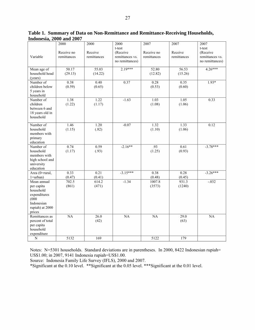
Table 1 presents summary data from IFLS 3 (2000) and IFLS 4 (2007). It shows that the

number of households receiving international remittances in Indonesia is fairly small: in 2000,

169 households (3.2 percent of all households) receive remittances, and in 2007, 179 households

(3.3 percent of all households) receive remittances.4 According to the table, households

receiving international remittances in Indonesia have older household heads, have fewer

household members with high school and university education, and are more likely to be located

in rural areas. Households receiving international remittances also tend to have lower mean per

capita expenditures than households without remittances. For households receiving remittances,

remittances represent 26.0 percent of total household expenditures in 2000 and 29.0 percent of

expenditures in 2007. However, since households receiving international remittances in

Indonesia also have low levels of expenditure, the absolute amount of remittances received in

annual per capita terms by households is quite low: not exceeding US $30 in either year.5

8

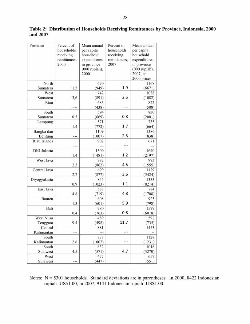
Table 2 shows the distribution of households receiving international remittances by

province in Indonesia. The data show that the share of households receiving remittances is fairly

small in all provinces except for one rural province: West Nusa Tenggara. In terms of mean

annual per capita household expenditures, West Nusa Tenggara province is also one of the

poorest provinces in the sample.

2. An Econometric Model of Household Incomes with Selection Controls

Since most poverty economists use expenditure rather than income data to identify

poverty,6 it is tempting to use the mean per capita expenditure figures from Tables 1 and 2 to

conclude that households receiving international remittances in Indonesia are more likely to be

poor.7 However, it is important to realize that these expenditure figures are “naïve” and cannot

be used to evaluate the “real” effect of remittances on poverty in Indonesia. Households have

both observed and unobserved characteristics. Since the expenditure results in Tables 1 and 2

may be caused by the unobserved characteristics of households (e.g. skills, motivation, ability), it

is important to use special econometric techniques to identify the impact of these unobservables

in order to pinpoint the “real” impact of remittances on expenditures and poverty in Indonesia.

Specifically, it is necessary to estimate a counterfactual scenario in which we estimate the

expenditures for households that receive international remittances, and then compare these

expenditures with an unobserved scenario in which these households do not receive remittances.

Constructing such a counterfactual can be done by treating households with no remittances as a

random draw from the population, estimating a mean regression of incomes for these no-

remittance households, and then using the resulting parameter estimates to predict the incomes of

households with international remittances. However, this approach becomes problematic if

9

households with and without remittances differ systematically in their unobservable

characteristics (e.g. skills, motivation, ability), because then the regression results will be biased.

The approach followed in this paper is to estimate an equation for households receiving

international remittances, taking into account in the estimation the selection bias. This kind of

approach is based on a selection model developed by Dubin and McFadden (1984) and

Bourguignon, Fournier and Gurgand (2004).8

The estimation strategy of this paper is to use a three-stage model to estimate

counterfactual expenditures for households receiving remittances taking into account selection

bias. The first-stage uses a nested logit with instrumental variables to estimate the probability of

households receiving remittances. The second-stage uses a generalization of the Dubin and

McFadden model (1984) to estimate selection-corrected household expenditures with and

without remittances. The third stage estimates the value of the fixed effects and undifferenced

selection terms. More specifically, our estimation strategy can be developed as follows.

Our panel data from Indonesia is for two years (2000 and 2007) and this gives us certain

advantages over simple cross-sectional data. For example, we know whether households have

chosen to receive remittances in each of four states: (1) no remittances in either year; (2)

remittances in 2000 but not in 2007; (3) remittances in both years, 2000 and 2007; and (4)

remittances in 2007 but not in 2000. Moreover, some of the characteristics of our households are

fixed, and thus do not change according to their remittance situation, while other unobservable

characteristics change depending on how the households choose between the four states.

For example, assume that in time period 1, households can select between two states (r):

(1) receive no remittances; (2) receive remittances. Once households have chosen their state,

they decide their level of expenditure ytr, where ytr is the optimal expenditure for households that

10

chose r=r. At time period 2, conditional on their state (r), they can again select between two

states (r): (1) receive no remittances; (2) receive remittances. Once households have chosen their

state, they decide their level of expenditure ytr. We assume that this decision tree is represented

by a nested logit process. Moreover, we assume that at time 1 there are two expenditure

equations:

Ytri = βr(1-d2) + arX1i+αi+utri (1)

Where d2 is a dummy that is 1 for time period 2, and it is zero for time period 1. αi

represents the individual fixed effect. From this point on, we will not mention the subscript for

household i in the paper. For time period 2, this decision structure generates the four types of

households mentioned above: (1) those that never receive remittances; (2) those that switch from

not having remittances in 2000 to receiving remittances in 2007; (3) those that always receive

remittances; and (4) those that switch from receiving remittances in 2000 to not receiving them

in 2007. For households that do not switch in their remittance state between 2000 and 2007 (i.e.

households (1) and (3)) we can obtain the first difference and get:

ΔYr = βr +a rΔX + Δur (2)

Under the assumption of a nested logit, it can be shown that Δur can be represented as a

linear combination of all available possibilities at the final stage of the nested logit tree:

ΔYr = βr +a rΔX +∑ +vr (3)

Where the represent the probabilities of all final possibilities at the final stage of the

nested logit tree, with the exception of option r. Equation (3) implies that we can estimate the

coefficients for the expenditure equation of households that select option r and never switch their

remittance state based only on the observations of such households.

11

For households that switch their remittance state between 2000 and 2007 we can write the

first difference as:

Y2r- Y1r’ = - βr’ +arX2i-ar’X1i +ur -ur’ (4)

There are only k=2 transitions that can be made in the model: (1) from receiving no

remittances in 2000 to having remittances in 2007; and (2) from receiving remittances in 2000 to

not receiving them in 2007. Finally, and given that ur -ur’ represents one of the final possibilities

in the nested logit, we represent our equation as:

ΔYk = γk +λ kΔX +∑ +vk (5)

Consequently, we can estimate how the switches in remittance states are correlated to the

characteristics of the households. Moreover, the levels of expenditures for households in 2000

can be obtained as follows:

E(Y1r |X) = βr+ arX1+αi+E(u1r |X) (6)

For the case of households that do not switch their remittance state (that is, never receive

remittances or receive remittances in both years), the equation for their expected income in 2007

is:

E(Y2r|X) = arX1+αi+ E(u1r |X) + a rΔX +∑ (7)

For the case of households that switch their remittance state (that is, switch from not

receiving remittances to receiving remittances, or vice versa) the equation for their expected

income in 2007 is:

E(Y2k|X) = arX1+αi+ E(u1r |X) +λ kΔX +∑ (8)

Notice that equations (6), (7) and (8) give us two elements that need to be determined

simultaneously αi and E(u1r |X). This is done using a search procedure where we use the fact

12

that we have a nested logit to express E(u1r |X) =θrpr. The search procedure consists in finding a

set of θr and αi that simultaneously satisfy equations (6), (7) and (8).

To implement our estimation, the first stage model consists in estimating the probabilities to

be in any part of the decision tree in 2000 and 2007, using a nested logit specification. To

identify this part of the model, we need instrumental variables that enter the first stage model, but

not the second stage. In our case, these instrumental variables are three: (1) the distance from

kabupaten (district) to railroad station in 1930; (2) the level of rainfall in 1995-1999; and (3)

unexpected rainfall in 2000.9 Our rationale for using these three instrumental variables is as

follows.

The first railroad line in Indonesia opened in 1867. A continuous railroad line between

Jakarta and Surabaya, the two largest cities in Java, opened in 1894. Between 1900 and 1930

smaller railroad lines were constructed in Madura, Sumatra and South Celebes. In Indonesia

distance to railroad lines in 1930 represents a good instrumental variable because it is related to

migration costs in the past and to the need for sending migrants in the past, and therefore to the

development of present day migrant social networks, but it is not correlated with the expenditure

patterns of households at the time of the 2000 and 2007 IFLS Surveys. We calculated distance to

railroad lines for each household using the distance from the kabupaten (district) to the nearest

railroad station in 1930, using historical maps from the Indonesian Railway Authority, and then

cross-checking this information with the IFLS Surveys. This type of instrument has been used

before in the literature by Woodruff and Zenteno (2007) for the case of Mexico, and Adams and

Cuecuecha (forthcoming) for the case of Guatemala.

Changes in rainfall have also been used before in the literature as an instrumental variable

in the cases of Mexico, the Philippines, and Guatemala (Munshi, 2003; Yang and Choi, 2007;

13

Adams and Cuecuecha, forthcoming). The argument here is that rain is closely correlated with

agricultural production and income, and so too little rain in one or several years may cause

people to migrate out of rural areas. For this reason, changes in historical rain are correlated

with the formation of migrant networks and with the receipt of remittances, but changes in

historical rain are not correlated with unobserved changes in consumption patterns. We obtained

historical rainfall information at the meteorological station level in Indonesia from the IFLS data.

We then calculated the average level of rainfall for the year 2000 and the average level of rainfall

for the period 1995 to 1999 by district. From this information we estimated a model in which the

level of rainfall for the year 2000 is related to the level of rainfall for the period 1995 to 1999.

We then used the residuals from this model as the unexpected rainfall shock in 2000. Our

argument here is that changes in migration patterns and the receipt of remittances are influenced

by both the unexpected part of rainfall in 2000 as well as the actual level of rainfall for 1995 to

1999, since both variables are exogenous at the beginning of the decision process estimated with

our data.

For the three instrumental variables, our claim is that conditional on the set of human

capital, household and district characteristics included in our specification, the unobserved

components in the expenditure equation of the households are uncorrelated with the three

instruments.

The second stage of our model estimates equation (3) and (5) using a generalization of

the Dubin and McFadden method, assuming a nested logit specification for the probabilities

needed in estimation.

The third stage of our model consists in estimating the values of the fixed effects. To

obtain the fixed effects we implement a search method using the following three steps. First, we

14

use the values of equations (3) and (5) in equations (6), (7) and (8) to obtain values for the fixed

effects and to obtain the average. In this first step we assume that θ=1. Second, we obtain θr and

αi from the regressions (9), (10) and (11):

Y1ri - βr - arX1i = αi0 + θpri +η1 (9)

Y2ri - arX1 - a rΔX - ∑ = αi0 + θrpri + η2 (10)

Y2ri - arX1 - λ kΔX - ∑ = αi0 + θrpri + η2 (11)

We then re-estimate the fixed effect for the above equations and obtain a new average αi1,

and compare it to the previous fixed effect. If the difference between αi1 and αi0 is above a

threshold, we repeat the procedure.

Third, once differences are lower than a threshold (i.e. convergence is achieved) we

declare our estimations for the fixed effects and θr to be our final estimations for those

parameters. On the basis of the preceding, our estimated expenditure for households that do not

switch their remittance state (that is, never receive remittances or receive remittances in both

years) is given by:

E(Y2r|X) = arX1+αi+ θrpri + a rΔX +∑ (12)

For the case of households that switch their remittance state (that is, switch from not

receiving remittances to receiving remittances, or vice versa) the equation for their expected

income in 2007 is:

E(Y2k|X) = arX1+αi+ θrpri +λ kΔX +∑ (13)

In the third stage of the model we also obtain the following two counterfactuals:10

1. The first counterfactual compares households receiving remittances in both years

(2007 and 2000) with their counterfactual income should they have switched from

15

receiving remittances in 2000 to not receiving remittances in 2007. Therefore, we use

for the counterfactual the equation for households that receive remittances in 2000,

but not in 2007.

2. The second counterfactual compares households receiving remittances in 2007 but

not in 2000 with their counterfactual income should they have not have received

remittances in 2007. Therefore, we use for the counterfactual the equation for

households that did not receive remittances in 2000, and that did not receive

remittances in 2007.

3. Estimating the Econometric Model with Selection Controls

Table 3 shows the results for the first-stage nested logit. The tree structure for the nested

logit assumes that households plan first whether or not to receive international remittances in

2000 and then conditional on their choice in 2000, choose their remittance state in 2007. In the

initial tree branch it is assumed that all variables are the ones shown in the table plus a dummy

variable for urban/rural areas and dummy variables for four Indonesian regions. The only

variable in the bottom branch of the nested logit is the instrumental variable, distance from

kabupaten (district) to railroad in 1930. The nested logit is estimated by partitioning the data by

the variable, age of household head, to help the equation converge.

In Table 3 two of the household characteristics are significantly related to the receipt of

remittances in 2007: age of household head and sex of household head. The sign on the age of

household head variable suggests that as the age of head increases, households are less likely to

receive remittances. The sign on the sex of household head variable suggests that female-headed

households are more likely to receive remittances.

16

In Table 3 one of the instrumental variables, distance from kabupaten (district) to

railroad, is also negatively and significantly related to the receipt of remittances in 2007. This

suggests that households living further away from a railroad in 1930 are less likely to receive

international remittances in 2007.

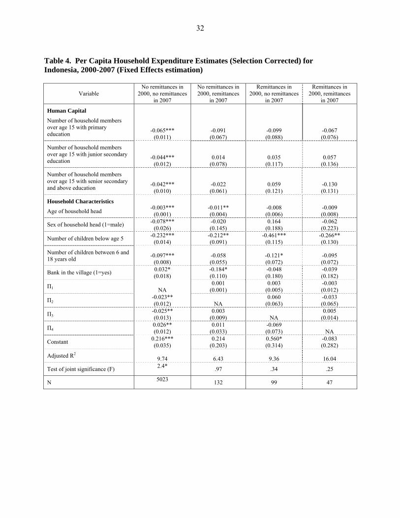
Table 4 shows the results for the second-stage expenditure equation. This table is based

on a fixed-effects estimation and partitions the households into the previously-discussed four

groups: (1) households never receiving remittances; (2) households receiving remittances in

2000 but not in 2007; (3) households not receiving remittances in 2000 but receiving in 2007;

and (4) households receiving remittances in both years. With respect to the household

characteristic variables, many of the coefficients are statistically significant and suggest (as

expected) that households with older household heads and more children under age 5 have lower

per capita expenditures.

The selection term in Table 4 is the Π variable. This selection term is statistically

significant only for households that never receive remittances. This result suggests that some

unobserved household characteristics change over time for households that never receive

remittances.11

4. Estimating Predicted and Counterfactual Expenditure Functions

This section discusses how counterfactual expenditure estimates for households can be

developed by using predicted expenditure equations to identify the expenditures of households

with and without international remittances. The methodology for obtaining these estimates

follows the literature on the evaluation of programs for the case in which instrumental variables

are available (Maddala, 1983; Wooldridge, 2002).

17

The methodology includes three steps. First, we start with observed expenditures,

meaning the levels of expenditures reported by households in the survey. Second, we obtain

predicted expenditures for households receiving remittances conditional on their household

characteristics and their choice of receiving remittances. Third, we obtain counterfactual

expenditures for households receiving remittances conditional on their household characteristics

and the hypothetical condition in which they do not receive remittances. We then use pairwise

Average Treatment Effects on the Treated (ATT) to compare counterfactual expenditures for

households receiving remittances using the following two steps.

1. The first ATT compares households receiving remittances in both years (2007 and

2000) with their counterfactual expenditure should they have switched to not

receiving remittances in 2007. Therefore, we use for the counterfactual the equation

for households that receive remittances in 2000, but not in 2007. The counterfactual

equation in this case is given by:12

E(YCF2k|X) = arX1+αi+ θrpri +λ kΔX +∑ (14)

Therefore, the effect of remittances on income, conditional on X is given by (that is,

by subtracting equation 14 from equation 12):

E(Y2r|X) - E(YCF2k|X) = (a r- λ k)ΔX +∑ (15)

2. The second ATT compares households receiving remittances in 2007 but not in 2000

with their counterfactual expenditure should they have not received remittances in

2007. Therefore, we use for the counterfactual the equation for households that did

18

not receive remittances in 2000, and did not receive remittances in 2007. The

counterfactual equation in this case is given by:

E(YCF2r|X) = arX1+αi+ θrpri + a rΔX +∑ (16)

Therefore, the effect of remittances on expenditure for these households is given by

(that is, subtracting equation 16 from equation 13):

E(Y2k|X) - E(YCF2r|X) = (λ k- a r)ΔX +∑ (17)

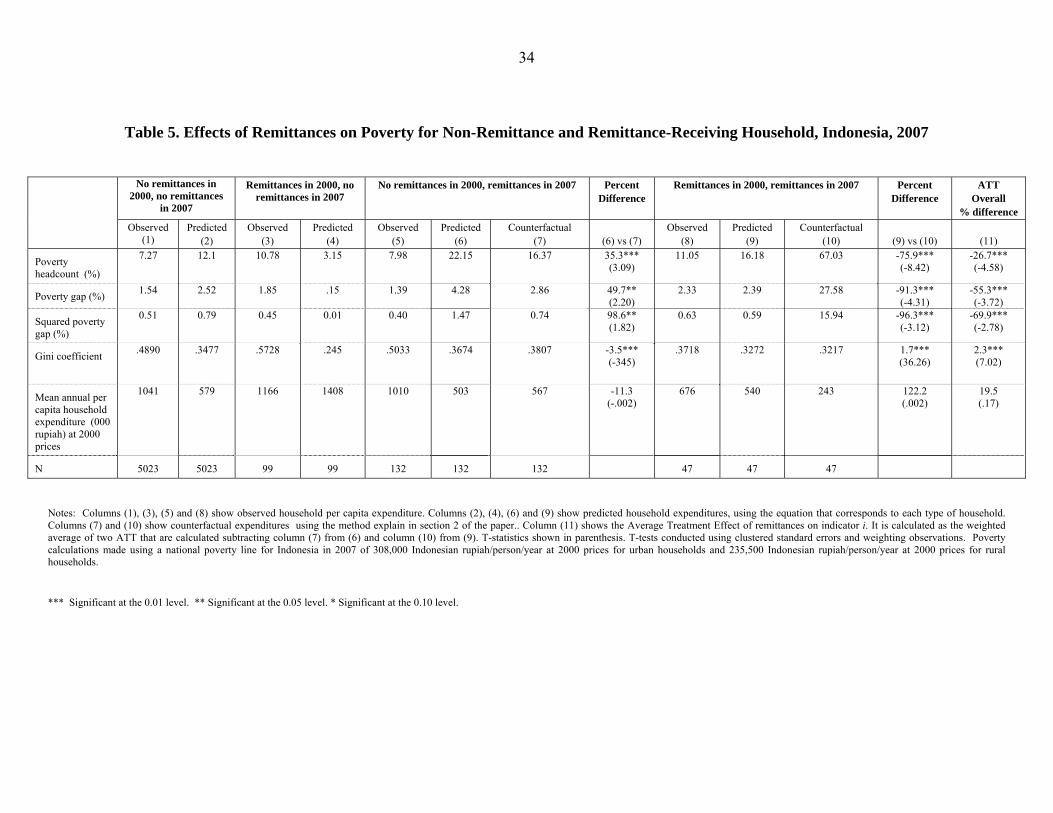
5. Expenditures, Remittances and Poverty

Table 5 reports observed, predicted and counterfactual expenditures for the four groups

of households: households never receiving remittances, households receiving remittances in

2000 but not in 2007, households not receiving remittances in 2000 but receiving in 2007, and

households receiving remittances in both years. On the basis of these expenditure levels, the

table also reports levels of poverty based on a 2007 national poverty line for Indonesia of

308,000 rupiah/person/year at 2000 prices for urban households, and 235,500 rupiah/person/year

at 2000 prices for rural households.13

Three different poverty measures appear in Table 5. The first measure -- the poverty

headcount -- shows the percent of the population living beneath the poverty line. However, this

headcount index ignores the “depth of poverty,” that is, the amount by which the average

expenditure of the poor fall short of the poverty line. The table therefore reports a second

measure, the poverty gap. This index measures in percentage terms how far the average

expenditures of the poor fall short of the national poverty line. The third poverty measure -- the

squared poverty gap – shows the “severity of poverty.” The squared poverty gap index possesses

useful analytical properties, because it is sensitive to changes in distribution among the poor. In

19

other words, while a transfer of expenditures from a poor person to a poorer person will not

change the headcount index or the poverty gap index, it will decrease the squared poverty gap

index.14

Columns (1) and (2) of Table 5 show that households which never receive international

remittances have mean per capita expenditures that situate them in the middle of the expenditure

distribution of Indonesia. For this reason, households which never receive remittances have the

lowest amount of observed poverty on average in the table.

By contrast, columns (8) and (9) show that households which receive international

remittances in both years (2000 and 2007) have the lowest mean per capita expenditures in the

table and the highest rates of observed poverty on average in the table.

In Table 5 it is possible to identify the impact of remittances on poverty by comparing the

results for predicted poverty values with those for counterfactual poverty. Specifically, for

households receiving remittances in 2007, but not in 2000, it is possible to compare predicted

poverty in column (6) with counterfactual poverty in column (7), and for households receiving

remittances in both years (2000 and 2007) columns (9) and (10) can be compared. Results

suggest that for households receiving remittances in 2007, but not in 2000, the receipt of

remittances increases the poverty headcount by 35.3 percent, but that for households receiving

remittances in both 2000 and 2007 the receipt of remittances decreases the poverty headcount by

75.9 percent.

While these results may appear contradictory and inconclusive, when we calculate overall

Average Treatment Effects on the Treated (ATT) the effect of receiving remittances on poverty

becomes clearer.15 In calculating the overall ATT we average the poverty results for households

receiving remittances in both years with the poverty results for households receiving remittances

20

only in 2007. This overall ATT uses the ATT for households receiving remittances in 2007 and

compares it to the counterfactual that would occur if these households did not receive

remittances in 2007. Results for the overall ATT in column (11) in Table 5 show that all three of

the poverty measures – poverty headcount, poverty gap and squared poverty gap -- show a large

and statistically significant decrease. According to column (11), the poverty headcount declines

by 26.7 percent, the poverty gap falls by 55.3 percent and the squared poverty gap falls by 69.9

percent. On the basis of these findings, international remittances appear to have a large,

statistical effect on reducing poverty in Indonesia

However, Table 5 shows that international remittances increase income inequality in

Indonesia. For households receiving remittances in 2007, but not in 2000, the Gini coefficient of

inequality falls by 3.5 percent with the receipt of remittances, while for households receiving

remittances in both years (2000 and 2007) the Gini coefficient rises by 1.7 percent. In column

(11) the overall ATT for the Gini coefficient shows that the Gini increases by 2.3 percent, and

that this increase is statistically significant.

6. Estimating the Marginal Expenditure Behavior of Households

Since we want to examine the impact of remittances on expenditures, it is important to

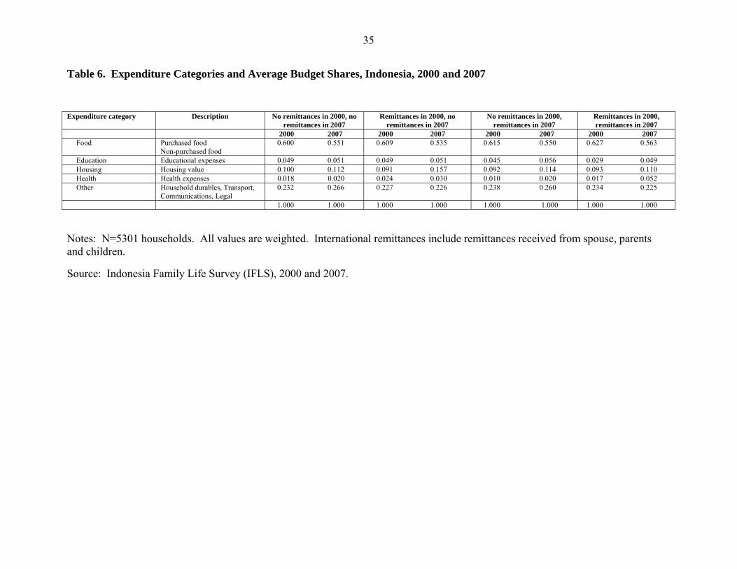
present the type of expenditure data contained in the IFLS Survey (2000 and 2007). Table 6

shows that the survey collected detailed information on five major categories of expenditure, and

on several subdivisions within each category. While the time base over which these expenditure

outlays were measured varied (from last 7 days for most food items, to last year for most durable

goods), all expenditures were aggregated to obtain yearly values. For household durables (stove,

refrigerator, automobile, etc), annual use values were calculated to obtain an estimate of the cost

21

of one year’s use of that good. Annual use values were also calculated to obtain an estimate of

the one year use value of housing (rented or owned).

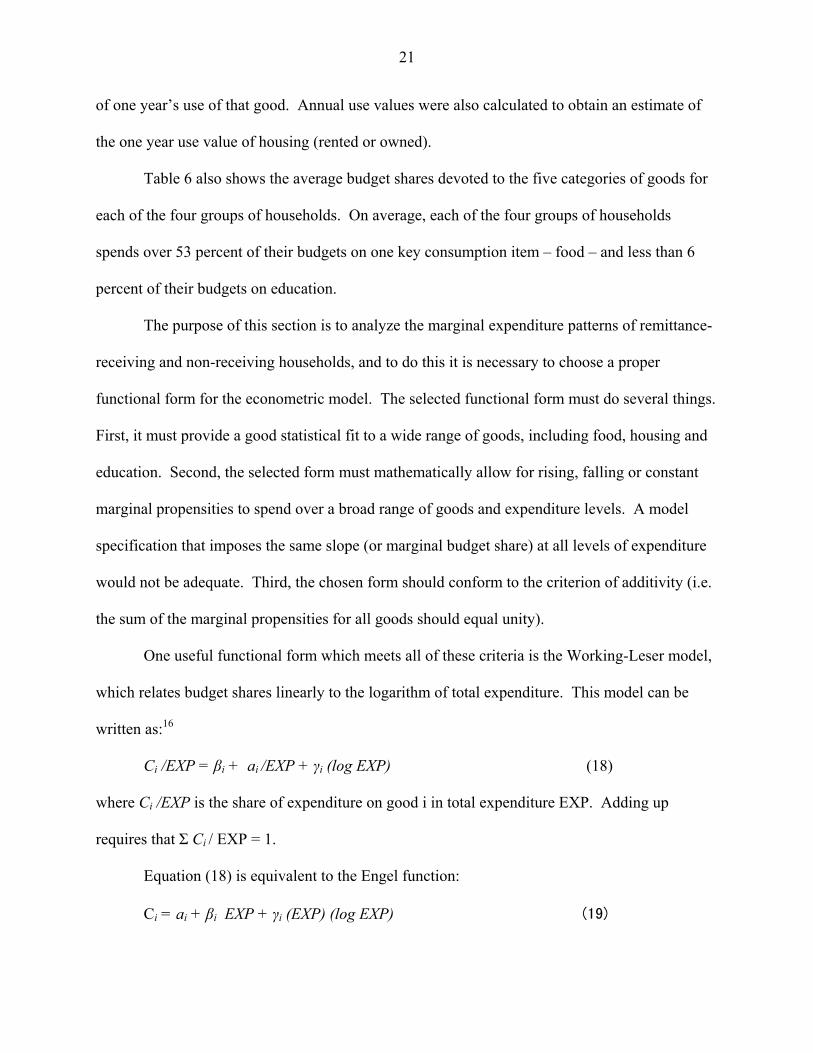
Table 6 also shows the average budget shares devoted to the five categories of goods for

each of the four groups of households. On average, each of the four groups of households

spends over 53 percent of their budgets on one key consumption item – food – and less than 6

percent of their budgets on education.

The purpose of this section is to analyze the marginal expenditure patterns of remittance-

receiving and non-receiving households, and to do this it is necessary to choose a proper

functional form for the econometric model. The selected functional form must do several things.

First, it must provide a good statistical fit to a wide range of goods, including food, housing and

education. Second, the selected form must mathematically allow for rising, falling or constant

marginal propensities to spend over a broad range of goods and expenditure levels. A model

specification that imposes the same slope (or marginal budget share) at all levels of expenditure

would not be adequate. Third, the chosen form should conform to the criterion of additivity (i.e.

the sum of the marginal propensities for all goods should equal unity).

One useful functional form which meets all of these criteria is the Working-Leser model,

which relates budget shares linearly to the logarithm of total expenditure. This model can be

written as:16

Ci /EXP = βi + ai /EXP + γi (log EXP) (18)

where Ci /EXP is the share of expenditure on good i in total expenditure EXP. Adding up

requires that Σ Ci / EXP = 1.

Equation (18) is equivalent to the Engel function:

Ci = ai + βi EXP + γi (EXP) (log EXP) (19)

22

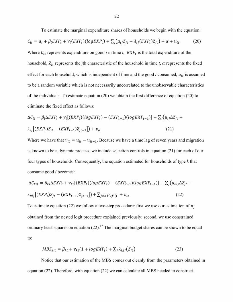
To estimate the marginal expenditure shares of households we begin with the equation:

∑ (20)

Where represents expenditure on good i in time t, is the total expenditure of the

household, represents the jth characteristic of the household in time t, represents the fixed

effect for each household, which is independent of time and the good i consumed, is assumed

to be a random variable which is not necessarily uncorrelated to the unobservable characteristics

of the individuals. To estimate equation (20) we obtain the first difference of equation (20) to

eliminate the fixed effect as follows:

∆ ∆ ∑ ∆

(21)

Where we have that . Because we have a time lag of seven years and migration

is known to be a dynamic process, we include selection controls in equation (21) for each of our

four types of households. Consequently, the equation estimated for households of type k that

consume good i becomes:

∆ ∆ ∑ ∆

∑ (22)

To estimate equation (22) we follow a two-step procedure: first we use our estimation of

obtained from the nested logit procedure explained previously; second, we use constrained

ordinary least squares on equation (22).17 The marginal budget shares can be shown to be equal

to:

1 ∑ (23)

Notice that our estimation of the MBS comes out cleanly from the parameters obtained in

equation (22). Therefore, with equation (22) we can calculate all MBS needed to construct

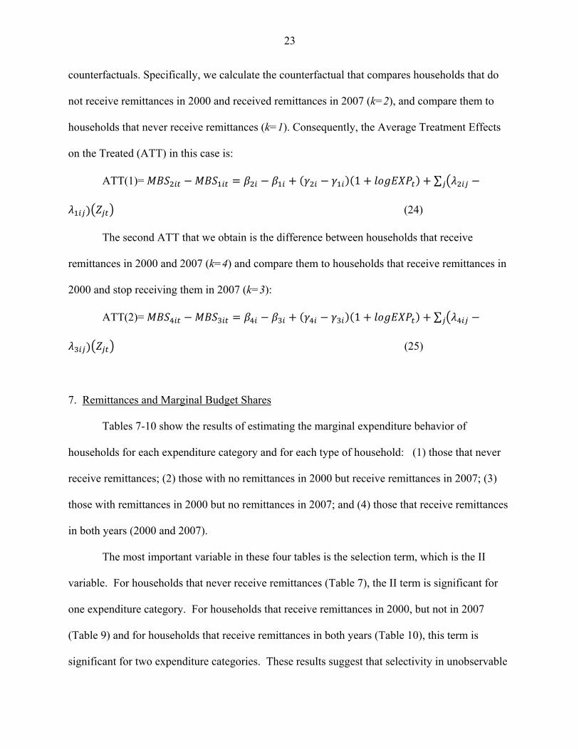
23

counterfactuals. Specifically, we calculate the counterfactual that compares households that do

not receive remittances in 2000 and received remittances in 2007 (k=2), and compare them to

households that never receive remittances (k=1). Consequently, the Average Treatment Effects

on the Treated (ATT) in this case is:

ATT(1)= 1 ∑

(24)

The second ATT that we obtain is the difference between households that receive

remittances in 2000 and 2007 (k=4) and compare them to households that receive remittances in

2000 and stop receiving them in 2007 (k=3):

ATT(2)= 1 ∑

(25)

7. Remittances and Marginal Budget Shares

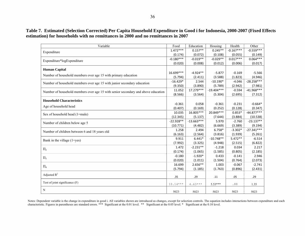
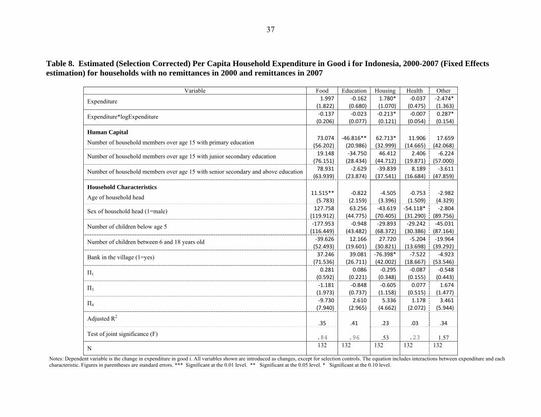
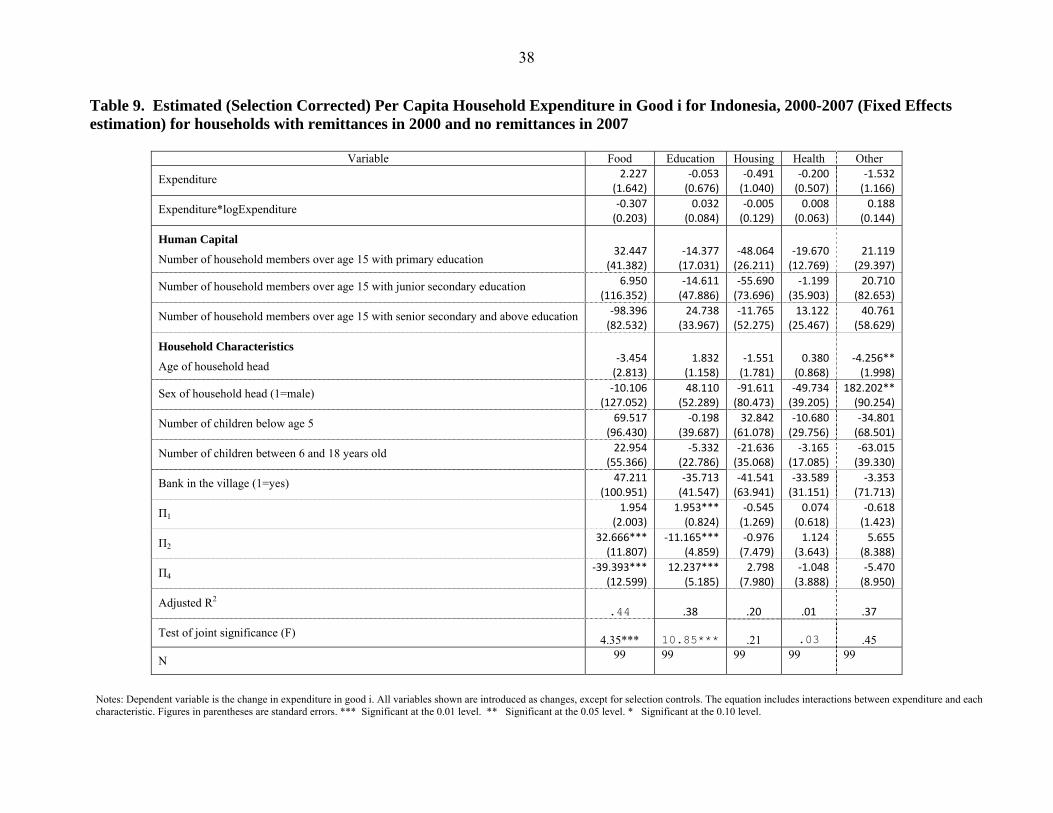
Tables 7-10 show the results of estimating the marginal expenditure behavior of

households for each expenditure category and for each type of household: (1) those that never

receive remittances; (2) those with no remittances in 2000 but receive remittances in 2007; (3)

those with remittances in 2000 but no remittances in 2007; and (4) those that receive remittances

in both years (2000 and 2007).

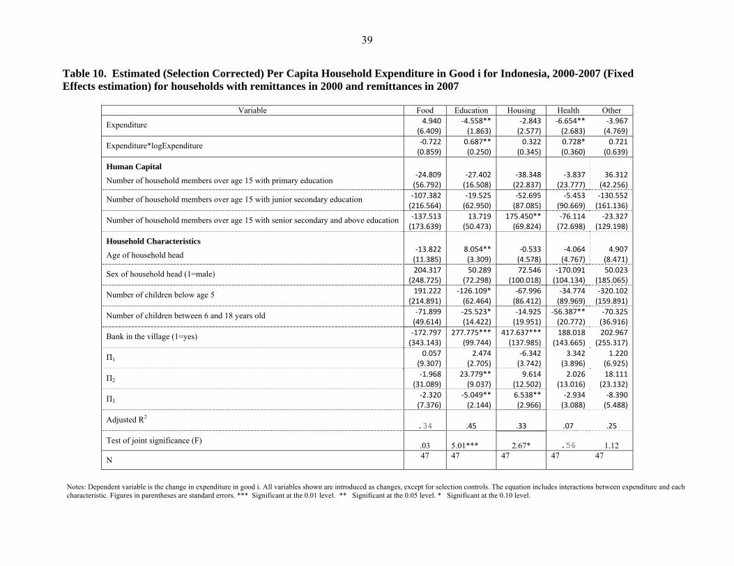
The most important variable in these four tables is the selection term, which is the II

variable. For households that never receive remittances (Table 7), the II term is significant for

one expenditure category. For households that receive remittances in 2000, but not in 2007

(Table 9) and for households that receive remittances in both years (Table 10), this term is

significant for two expenditure categories. These results suggest that selectivity in unobservable

24

components matters for households receiving international remittances in Indonesia. In other

words, estimations ignoring the selectivity part of the model would be biased.

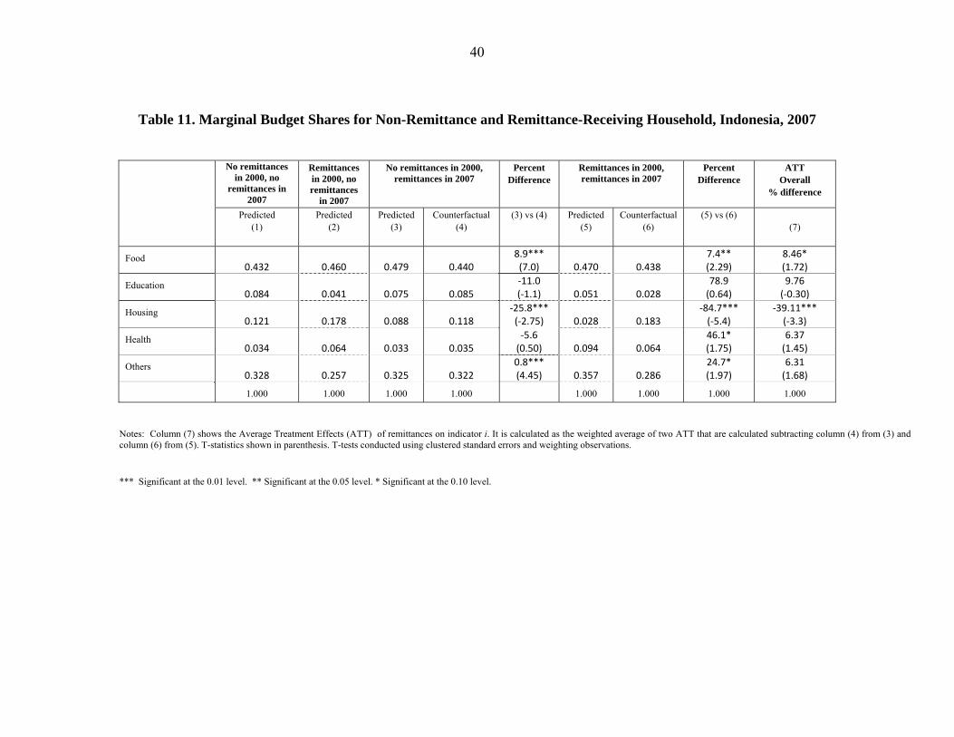
Table 11 takes the coefficients from Tables 7 to 10 and calculates the estimated and

counterfactual marginal budget shares for the five categories of expenditure for each type of

household. This table also shows the overall Average Treatment Effects on the Treated (ATT),

which averages the ATT for all households receiving remittances in 2007 and compares it to the

counterfactual of what would have happened if these households did not receive remittances in

2007.18

Three of the ATT results in Table 11 (column 7) are noteworthy. First, compared to a

counterfactual situation in which they did not receive international remittances in 2007,

households receiving remittances in 2007 spend more at the margin on one key consumption

good: food. Households receiving remittances in 2007 spend 8.5 percent more at the margin on

food than what they would have spent on this good without the receipt of remittances. Second,

compared to a counterfactual situation in which they did not receive international remittances in

2007, households receiving remittances in 2007 spend less at the margin on one important

investment good: housing. Households receiving remittances in 2007 spend 39.1 less at the

margin on housing than what they would have spent on this good without the receipt of

remittances. Finally, compared to a counterfactual situation in which they did not receive

international remittances in 2007, households receiving remittances in 2007 spend more at the

margin on education, but this result is not statistically significant.

8. Conclusion

This paper has used data from a large, panel household survey in Indonesia to analyze

25

the impact of international remittances on poverty and household consumption and investment.

The paper has three key findings, and two of these findings merit comment.

First, using an instrumental variables approach to control for selection and endogeneity,

the paper finds that international remittances have a large, statistical effect on reducing poverty

in Indonesia. When we compare households receiving international remittances in 2007 with a

counterfactual situation in which these households did not receive remittances in 2007, we find

that the poverty headcount falls by 26.7 percent and the squared poverty gap declines by 69.9

percent. These results are much larger than those produced by broader, cross-national studies on

the relationship between remittances and poverty. For example, Adams and Page (2005) find

that a 10 percent increase in international remittances in a country will lead, on average, to a 3.5

percent decline in the poverty headcount and a 2.8 percent decline in the squared poverty gap.

Second, when we compare households receiving remittances in 2007 with a

counterfactual situation in which they did not receive remittances in 2007, we find that

households receiving remittances increase their marginal expenditures on one key consumption

good – food – by 8.5 percent.

Third, when we compare households receiving international remittances in 2007 with a

counterfactual situation in which they did not receive remittances in 2007, we find that

households receiving remittances reduce their marginal expenditures on one key investment

good – housing – by 39.1 percent.

The second and third findings of this paper deserve comment because they are at odds

with recent research on the impact of remittances on consumption and investment in other

countries. For example, using a large, nationally-representative household data set and a similar

instrumental variables approach in Guatemala, Adams and Cuecuecha (forthcoming) find that

26

since remittances are a transitory type of income, that households tend to spend them more on

the margin on human and physical investment goods – like education and housing – than on

consumption goods – like food. The difference between these two sets of findings – Guatemala

and Indonesia – can be explained as follows. In Guatemala households receiving international

remittances receive much more in annual per capita terms from remittances than those in

Indonesia (US $365 vs. US $30 per year). As a result, mean annual per capita expenditure levels

for remittance-receiving households in Guatemala are much higher than those in Indonesia.19

Remittance-receiving households in Guatemala thus have more income and are able to devote

more of their marginal expenditures to investment in human and physical capital: education and

housing. By contrast, households receiving international remittances in Indonesia are much

poorer and thus the focus of their marginal expenditures is on improving their consumption of

basic goods – like food – rather than second-order investment goods, like education and housing.

In the future, as remittance-receiving households in Indonesia continue to raise their average per

capita expenditures through the receipt of international remittances, it is likely that they will

devote more of their marginal expenditures to these second-order investment goods.

27

Table 1. Summary of Data on Non-Remittance and Remittance-Receiving Households, Indonesia, 2000 and 2007 Variable

2000 Receive no remittances

2000 Receive remittances

2000 t-test (Receive remittances vs. no remittances)

2007 Receive no remittances

2007 Receive remittances

2007 t-test (Receive remittances vs. no remittances)

Mean age of household head (years)

50.17 (29.13)

55.03 (14.22)

2.19*** 52.80 (12.82)

56.53 (15.26)

4.26***

Number of children below 5 years in household

0.38 (0.59)

0.40 (0.65)

0.37 0.28 (0.53)

0.35 (0.60)

1.93*

Number of children between 6 and 18 years old in household

1.38 (1.22)

1.22 (1.17)

-1.63 1.03 (1.08)

1.05 (1.06)

0.33

Number of household members with primary education

1.46 (1.15)

1.20 (.82)

-0.07 1.32 (1.10)

1.33 (1.06)

0.12

Number of household members with high school and university education

0.74 (1.17)

0.59 (.93)

-2.16** .93 (1.25)

0.61 (0.93)

-3.78***

Area (0=rural, 1=urban)

0.33 (0.47)

0.21 (0.41)

-3.15*** 0.38 (0.48)

0.28 (0.45)

-3.26***

Mean annual per capita household expenditures (000 Indonesian rupiah) at 2000 prices

702.5 (861)

614.2 (471)

-1.34 1007.8 (3573)

931.3 (1240)

-.032

Remittances as percent of total per capita household expenditure

NA 26.0 (42)

NA NA 29.0 (63)

NA

N 5132 169 5122 179

Notes: N=5301 households. Standard deviations are in parentheses. In 2000, 8422 Indonesian rupiah= US$1.00; in 2007, 9141 Indonesia rupiah=US$1.00. Source: Indonesia Family Life Survey (IFLS), 2000 and 2007. *Significant at the 0.10 level. **Significant at the 0.05 level. ***Significant at the 0.01 level.

28

Table 2: Distribution of Households Receiving Remittances by Province, Indonesia, 2000 and 2007 Province Percent of

households receiving remittances, 2000

Mean annual per capita household expenditures in province (000 rupiah), 2000

Percent of households receiving remittances, 2007

Mean annual per capita household expenditures in province (000 rupiah), 2007, at 2000 prices

North Sumatera

1.5

670 (949) 1.9

1168 (6671)

West Sumatera

3,6

742 (891) 2.5

1038 (1082)

Riau ---

683 (438) ‐‐‐

822 (508)

South Sumatera

0.3

594 (669) 0.8

830 (2001)

Lampung 1.4

571 (772) 1.7

735 (664)

Bangka dan Belitung ---

1109 (1007) 2.5

1386 (838)

Riau Islands ---

902 --- ‐‐‐

671 ---

DKI Jakarta 1.4

1300 (1481) 1.2

1640 (2197)

West Java 2.3

782 (862) 4.5

993 (1555)

Central Java 2.7

699 (877) 3.6

1129 (5424)

Diyogyakarta 0.9

845 (1023) 1.1

1333 (8214)

East Java 4.8

588 (719) 4.8

784 (1708)

Banten 1.3

608 (601) 5.9

923 (798)

Bali 0.4

780 (763) 0.8

1599 (6018)

West Nusa Tenggara 9.4

489 (498) 11.7

592 (735)

Central Kalimantan ---

881 --- ‐‐‐

1453 --

South Kalimantan 2.6

778 (1002) ‐‐‐

1128 (1231)

South Sulawesi 4.5

632 (571) 4.7

1018 (3270)

West Sulawesi ---

477 (447) ‐‐‐

657 (551)

Notes: N = 5301 households. Standard deviations are in parentheses. In 2000, 8422 Indonesian rupiah=US$1.00; in 2007, 9141 Indonesian rupiah=US$1.00.

29

Table 2: Distribution of Households Receiving Remittances by Province, Indonesia, 2000 and 2007 Source: Indonesia Family Life Survey (IFLS), 2000 and 2007.

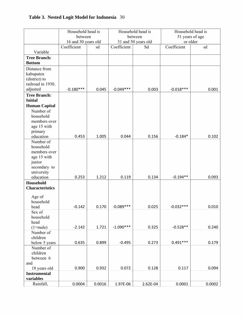
Table 3. Nested Logit Model for Indonesia 30

Household head is between

16 and 30 years old

Household head is between

31 and 50 years old

Household head is 51 years of age

or older

Variable Coefficient sd Coefficient Sd Coefficient sd

Tree Branch: Bottom

Distance from kabupaten (district) to railroad in 1930, adjusted ‐0.180*** 0.045 ‐0.049*** 0.003 ‐0.018*** 0.001

Tree Branch: Initial Human Capital

Number of household members over age 15 with primary education 0.453 1.005 0.044 0.156 ‐0.184* 0.102Number of household members over age 15 with junior secondary to university education 0.253 1.212 0.119 0.134 ‐0.194** 0.093

Household Characteristics

Age of household head ‐0.142 0.170 ‐0.089*** 0.025 ‐0.032*** 0.010Sex of household head (1=male) ‐2.142 1.721 ‐1.090*** 0.325 ‐0.528** 0.240Number of children below 5 years 0.635 0.899 ‐0.495 0.273 0.491*** 0.179

Number of children between 6 and 18 years old 0.900 0.932 0.072 0.128 0.117 0.094

Instrumental variables Rainfall, 0.0004 0.0016 1.97E‐06 2.62E‐04 0.0001 0.0002

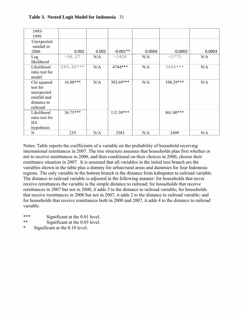
Table 3. Nested Logit Model for Indonesia 31

1995- 1999 Unexpected rainfall in 2000 0.002 0.002 ‐0.001** 0.0004 ‐0.0003 0.0003

Log likelihood

-56.27 N/A -1426 N/A -1773 N/A

Likelihood ratio test for model

283.92*** N/A 4744*** N/A 3406*** N/A

Chi squared test for unexpected rainfall and distance to railroad

16.88*** N/A 303.69*** N/A 198.29*** N/A

Likelihood ratio test for IIA hypothesis

36.75*** 112.38*** 861.80***

N 219 N/A 2583 N/A 2499 N/A

Notes: Table reports the coefficients of a variable on the probability of household receiving international remittances in 2007. The tree structure assumes that households plan first whether or not to receive remittances in 2000, and then conditional on their choices in 2000, choose their remittance situation in 2007. It is assumed that all variables in the initial tree branch are the variables shown in the table plus a dummy for urban/rural areas and dummies for four Indonesia regions. The only variable in the bottom branch is the distance from kabupaten to railroad variable. The distance to railroad variable is adjusted in the following manner: for households that never receive remittances the variable is the simple distance to railroad; for households that receive remittances in 2007 but not in 2000, it adds 3 to the distance to railroad variable; for households that receive remittances in 2000 but not in 2007, it adds 2 to the distance to railroad variable; and for households that receive remittances both in 2000 and 2007, it adds 4 to the distance to railroad variable. *** Significant at the 0.01 level. ** Significant at the 0.05 level. * Significant at the 0.10 level.

32

Table 4. Per Capita Household Expenditure Estimates (Selection Corrected) for Indonesia, 2000-2007 (Fixed Effects estimation)

Variable No remittances in

2000, no remittances in 2007

No remittances in 2000, remittances

in 2007

Remittances in 2000, no remittances

in 2007

Remittances in 2000, remittances

in 2007

Human Capital

Number of household members over age 15 with primary education

-0.065*** (0.011)

-0.091 (0.067)

-0.099 (0.088)

-0.067 (0.076)

Number of household members over age 15 with junior secondary education

-0.044*** (0.012)

0.014 (0.078)

0.035 (0.117)

0.057 (0.136)

Number of household members over age 15 with senior secondary and above education

-0.042*** (0.010)

-0.022 (0.061)

0.059 (0.121)

-0.130 (0.131)


Age of household head -0.003***

(0.001) -0.011** (0.004)

-0.008 (0.006)

-0.009 (0.008)

Sex of household head (1=male) -0.078*** (0.026)

-0.020 (0.145)

0.164 (0.188)

-0.062 (0.223)

Number of children below age 5 -0.232*** (0.014)

-0.212** (0.091)

-0.461*** (0.115)

-0.266** (0.130)

Number of children between 6 and 18 years old

-0.097*** (0.008)

-0.058 (0.055)

-0.121* (0.072)

-0.095 (0.072)

Bank in the village (1=yes) 0.032* (0.018)

-0.184* (0.110)

-0.048 (0.180)

-0.039 (0.182)

Π1 NA 0.001

(0.001) 0.003

(0.005) -0.003 (0.012)

Π2 -0.023** (0.012) NA

0.060 (0.063)

-0.033 (0.065)

Π3 -0.025** (0.013)

0.003 (0.009) NA

0.005 (0.014)

Π4 0.026** (0.012)

0.011 (0.033)

-0.069 (0.073) NA

Constant 0.216*** (0.035)

0.214 (0.203)

0.560* (0.314)

-0.083 (0.282)

Adjusted R2 9.74 6.43 9.36 16.04

Test of joint significance (F) 2.4* .97 .34 .25

N 5023 132 99 47

33

Table 4. Per Capita Household Expenditure Estimates (contd) Notes: Dependent variable is the log of annual per capita household expenditure (including remittances). The regression included a dummy for area and a dummy for region. Figures in parentheses are standard errors.

*** Significant at the 0.01 level. ** Significant at the 0.05 level. * Significant at the 0.10 level.

34

Table 5. Effects of Remittances on Poverty for Non-Remittance and Remittance-Receiving Household, Indonesia, 2007

Notes: Columns (1), (3), (5) and (8) show observed household per capita expenditure. Columns (2), (4), (6) and (9) show predicted household expenditures, using the equation that corresponds to each type of household. Columns (7) and (10) show counterfactual expenditures using the method explain in section 2 of the paper.. Column (11) shows the Average Treatment Effect of remittances on indicator i. It is calculated as the weighted average of two ATT that are calculated subtracting column (7) from (6) and column (10) from (9). T-statistics shown in parenthesis. T-tests conducted using clustered standard errors and weighting observations. Poverty calculations made using a national poverty line for Indonesia in 2007 of 308,000 Indonesian rupiah/person/year at 2000 prices for urban households and 235,500 Indonesian rupiah/person/year at 2000 prices for rural households.


No remittances in 2000, no remittances

in 2007

Remittances in 2000, no remittances in 2007

No remittances in 2000, remittances in 2007 Percent Difference

Remittances in 2000, remittances in 2007 Percent Difference

ATT Overall

% difference

Observed (1)

Predicted (2)

Observed (3)

Predicted (4)

Observed (5)

Predicted (6)

Counterfactual (7)

(6) vs (7)

Observed (8)

Predicted (9)

Counterfactual (10)

(9) vs (10)

(11)

Poverty headcount (%)

7.27 12.1 10.78 3.15 7.98 22.15 16.37 35.3*** (3.09)

11.05 16.18 67.03

-75.9*** (-8.42)

-26.7*** (-4.58)

Poverty gap (%) 1.54 2.52 1.85 .15 1.39 4.28 2.86 49.7**

(2.20) 2.33 2.39 27.58

-91.3*** (-4.31)

-55.3*** (-3.72)

Squared poverty gap (%)

0.51 0.79 0.45 0.01 0.40 1.47 0.74 98.6** (1.82)

0.63 0.59

15.94

-96.3*** (-3.12)

-69.9*** (-2.78)

Gini coefficient

.4890 .3477 .5728 .245

.5033 .3674 .3807 -3.5*** (-345)

.3718 .3272 .3217

1.7*** (36.26)

2.3*** (7.02)

Mean annual per capita household expenditure (000 rupiah) at 2000 prices

1041 579 1166 1408 1010 503 567

-11.3 (-.002)

676 540 243 122.2 (.002)

19.5 (.17)

N 5023 5023 99 99 132 132 132 47 47 47

35

Table 6. Expenditure Categories and Average Budget Shares, Indonesia, 2000 and 2007

Expenditure category Description No remittances in 2000, no remittances in 2007

Remittances in 2000, no remittances in 2007

No remittances in 2000, remittances in 2007

Remittances in 2000, remittances in 2007

2000 2007 2000 2007 2000 2007 2000 2007 Food Purchased food

Non-purchased food 0.600 0.551 0.609 0.535 0.615 0.550 0.627 0.563

Education Educational expenses 0.049 0.051 0.049 0.051 0.045 0.056 0.029 0.049 Housing Housing value 0.100 0.112 0.091 0.157 0.092 0.114 0.093 0.110 Health Health expenses 0.018 0.020 0.024 0.030 0.010 0.020 0.017 0.052 Other Household durables, Transport,

Communications, Legal 0.232 0.266 0.227 0.226 0.238 0.260 0.234 0.225

1.000 1.000 1.000 1.000 1.000 1.000 1.000 1.000

Notes: N=5301 households. All values are weighted. International remittances include remittances received from spouse, parents and children.

Source: Indonesia Family Life Survey (IFLS), 2000 and 2007.

36

Table 7. Estimated (Selection Corrected) Per Capita Household Expenditure in Good i for Indonesia, 2000-2007 (Fixed Effects estimation) for households with no remittances in 2000 and no remittances in 2007

Variable Food Education Housing Health Other

Expenditure 1.472*** (0.174)

0.157**(0.072)

0.245**(0.108)

‐0.167***(0.055)

‐0.559***(0.149)

Expenditure*logExpenditure ‐0.180*** (0.020)

‐0.019**(0.008)

‐0.029**(0.012)

0.017***(0.006)

0.064***(0.017)

Human Capital

Number of household members over age 15 with primary education 16.699***

(5.794) ‐4.924**(2.411)

‐5.877(3.588)

‐0.169(1.823)

‐5.566(4.946)

Number of household members over age 15 with junior secondary education ‐16.429* (9.350)

2.544(3.890)

‐10.190*(5.789)

‐4.046(2.942)

‐28.258***(7.981)

Number of household members over age 15 with senior secondary and above education 11.052 (8.566)

17.279***(3.564)

‐19.404***(5.304)

‐0.594(2.695)

‐41.968***(7.312)


Age of household head ‐0.361 (0.407)

0.058(0.169)

‐0.361(0.252)

‐0.231(0.128)

‐0.664*(0.347)

Sex of household head (1=male) 10.035 (12.345)

16.805***(5.137)

20.849***(7.644)

0.853*(3.884)

‐44.877***(10.538)

Number of children below age 5 ‐22.928** (10.771)

‐13.663***(4.482)

5.970(6.669)

‐2.760(3.389)

‐23.137**(9.194)

Number of children between 6 and 18 years old 1.258 (6.163)

2.494(2.564)

6.758*(3.816)

‐3.302*(1.939)

‐27.341***(5.261)

Bank in the village (1=yes) 9.911 (7.992)

6.441*(3.325)

‐10.748**(4.948)

5.472**(2.515)

‐6.514(6.822)

Π2 1.472

(0.174) ‐2.231**(1.065)

‐1.218(1.585)

0.034(0.805)

2.217(2.185)

Π3 ‐0.180 (0.020)

‐1.920*(1.011)

0.433(1.504)

‐0.141(0.764)

2.946(2.073)

Π4 16.699 (5.794)

2.656**(1.185)

1.003(1.763)

‐0.067(0.896)

‐2.741(2.431)

Adjusted R2 .35 .29 .11 .05 .29

Test of joint significance (F)

10.14***

4.63***

5.53***

.88

1.35

N

5023

5023

5023

5023

5023

Notes: Dependent variable is the change in expenditure in good i. All variables shown are introduced as changes, except for selection controls. The equation includes interactions between expenditure and each characteristic. Figures in parentheses are standard errors. *** Significant at the 0.01 level. ** Significant at the 0.05 level. * Significant at the 0.10 level.

37

Table 8. Estimated (Selection Corrected) Per Capita Household Expenditure in Good i for Indonesia, 2000-2007 (Fixed Effects estimation) for households with no remittances in 2000 and remittances in 2007


Expenditure 1.997 (1.822)

‐0.162(0.680)

1.780*(1.070)

‐0.037(0.475)

‐2.474*(1.363)

Expenditure*logExpenditure ‐0.137 (0.206)

‐0.023(0.077)

‐0.213*(0.121)

‐0.007(0.054)

0.287*(0.154)

Human Capital

Number of household members over age 15 with primary education 73.074

(56.202) ‐46.816**(20.986)

62.713*(32.999)

11.906(14.665)

17.659(42.068)

Number of household members over age 15 with junior secondary education 19.148 (76.151)

‐34.750(28.434)

46.412(44.712)

2.406(19.871)

‐6.224(57.000)

Number of household members over age 15 with senior secondary and above education 78.931 (63.939)

‐2.629(23.874)

‐39.839(37.541)

8.189(16.684)

‐3.611(47.859)


Age of household head 11.515** (5.783)

‐0.822(2.159)

‐4.505(3.396)

‐0.753(1.509)

‐2.982(4.329)


63.256(44.775)

‐43.619(70.405)

‐54.118*(31.290)

‐2.804(89.756)

Number of children below age 5 ‐177.953 (116.449)

‐0.948(43.482)

‐29.893(68.372)

‐29.242(30.386)

‐45.031(87.164)

Number of children between 6 and 18 years old ‐39.626 (52.493)

12.166(19.601)

27.720(30.821)

‐5.204(13.698)

‐19.964(39.292)


39.081(26.711)

‐76.398*(42.002)

‐7.522(18.667)

‐4.923(53.546)

Π1 0.281

(0.592) 0.086

(0.221) ‐0.295(0.348)

‐0.087(0.155)

‐0.548(0.443)

Π3 ‐1.181 (1.973)

‐0.848(0.737)

‐0.605(1.158)

0.077(0.515)

1.674(1.477)

Π4 ‐9.730 (7.940)

2.610(2.965)

5.336(4.662)

1.178(2.072)

3.461(5.944)

Adjusted R2 .35 .41 .23

.03 .34

Test of joint significance (F)

.84

.96

.53

.23

1.57

N 132 132 132 132 132


38

Table 9. Estimated (Selection Corrected) Per Capita Household Expenditure in Good i for Indonesia, 2000-2007 (Fixed Effects estimation) for households with remittances in 2000 and no remittances in 2007



‐0.053(0.676)

‐0.491(1.040)

‐0.200(0.507)

‐1.532(1.166)


0.032(0.084)

‐0.005(0.129)

0.008(0.063)

0.188(0.144)

Human Capital

Number of household members over age 15 with primary education 32.447

(41.382) ‐14.377(17.031)

‐48.064(26.211)

‐19.670(12.769)

21.119(29.397)

Number of household members over age 15 with junior secondary education 6.950 (116.352)

‐14.611(47.886)

‐55.690(73.696)

‐1.199(35.903)

20.710(82.653)

Number of household members over age 15 with senior secondary and above education ‐98.396 (82.532)

24.738(33.967)

‐11.765(52.275)

13.122(25.467)

40.761(58.629)



1.832(1.158)

‐1.551(1.781)

0.380(0.868)

‐4.256**(1.998)

Sex of household head (1=male) ‐10.106 (127.052)

48.110(52.289)

‐91.611(80.473)

‐49.734(39.205)

182.202**(90.254)

Number of children below age 5 69.517 (96.430)

‐0.198(39.687)

32.842(61.078)

‐10.680(29.756)

‐34.801(68.501)

Number of children between 6 and 18 years old 22.954 (55.366)

‐5.332(22.786)

‐21.636(35.068)

‐3.165(17.085)

‐63.015(39.330)


‐35.713(41.547)

‐41.541(63.941)

‐33.589(31.151)

‐3.353(71.713)

Π1 1.954

(2.003) 1.953***(0.824)

‐0.545(1.269)

0.074(0.618)

‐0.618(1.423)

Π2 32.666*** (11.807)

‐11.165***(4.859)

‐0.976(7.479)

1.124(3.643)

5.655(8.388)

Π4 ‐39.393***

(12.599) 12.237***

(5.185) 2.798

(7.980) ‐1.048(3.888)

‐5.470(8.950)

Adjusted R2 .44 .38 .20

.01 .37

Test of joint significance (F) 4.35***

10.85***

.21

.03

.45

N 99 99 99 99 99


39

Table 10. Estimated (Selection Corrected) Per Capita Household Expenditure in Good i for Indonesia, 2000-2007 (Fixed Effects estimation) for households with remittances in 2000 and remittances in 2007



‐4.558**(1.863)

‐2.843(2.577)

‐6.654**(2.683)

‐3.967(4.769)


0.687**(0.250)

0.322(0.345)

0.728*(0.360)

0.721(0.639)

Human Capital

Number of household members over age 15 with primary education ‐24.809 (56.792)

‐27.402(16.508)

‐38.348(22.837)

‐3.837(23.777)

36.312(42.256)

Number of household members over age 15 with junior secondary education ‐107.382 (216.564)

‐19.525(62.950)

‐52.695(87.085)

‐5.453(90.669)

‐130.552(161.136)

Number of household members over age 15 with senior secondary and above education ‐137.513 (173.639)

13.719(50.473)

175.450**(69.824)

‐76.114(72.698)

‐23.327(129.198)



8.054**(3.309)

‐0.533(4.578)

‐4.064(4.767)

4.907(8.471)


50.289(72.298)

72.546(100.018)

‐170.091(104.134)

50.023(185.065)

Number of children below age 5 191.222 (214.891)

‐126.109*(62.464)

‐67.996(86.412)

‐34.774(89.969)

‐320.102(159.891)

Number of children between 6 and 18 years old ‐71.899 (49.614)

‐25.523*(14.422)

‐14.925(19.951)

‐56.387**(20.772)

‐70.325(36.916)

Bank in the village (1=yes) ‐172.797 (343.143)

277.775***(99.744)

417.637***(137.985)

188.018(143.665)

202.967(255.317)

Π1 0.057

(9.307) 2.474

(2.705) ‐6.342(3.742)

3.342(3.896)

1.220(6.925)

Π2 ‐1.968

(31.089) 23.779**(9.037)

9.614(12.502)

2.026(13.016)

18.111(23.132)

Π3 ‐2.320 (7.376)

‐5.049**(2.144)

6.538**(2.966)

‐2.934(3.088)

‐8.390(5.488)

Adjusted R2 .34 .45 .33

.07 .25

Test of joint significance (F) .03

5.01***

2.67*

.56

1.12

N 47 47 47 47 47


40

Table 11. Marginal Budget Shares for Non-Remittance and Remittance-Receiving Household, Indonesia, 2007

Notes: Column (7) shows the Average Treatment Effects (ATT) of remittances on indicator i. It is calculated as the weighted average of two ATT that are calculated subtracting column (4) from (3) and column (6) from (5). T-statistics shown in parenthesis. T-tests conducted using clustered standard errors and weighting observations.


No remittances in 2000, no

remittances in 2007

Remittances in 2000, no remittances

in 2007

No remittances in 2000, remittances in 2007

Percent Difference

Remittances in 2000, remittances in 2007

Percent Difference

ATT Overall

% difference

Predicted (1)

Predicted (2)

Predicted (3)

Counterfactual (4)

(3) vs (4) Predicted (5)

Counterfactual (6)

(5) vs (6) (7)

Food 0.432 0.460 0.479 0.440

8.9*** (7.0) 0.470 0.438

7.4** (2.29)

8.46* (1.72)

Education 0.084 0.041 0.075 0.085

‐11.0 (‐1.1) 0.051 0.028

78.9 (0.64)

9.76 (‐0.30)

Housing 0.121 0.178 0.088 0.118

‐25.8*** (‐2.75) 0.028 0.183

‐84.7*** (‐5.4)

‐39.11*** (‐3.3)

Health 0.034 0.064 0.033 0.035

‐5.6 (0.50) 0.094 0.064

46.1* (1.75)

6.37 (1.45)

Others 0.328 0.257 0.325 0.322

0.8*** (4.45) 0.357 0.286

24.7* (1.97)

6.31 (1.68)

1.000 1.000 1.000 1.000 1.000 1.000 1.000 1.000

41

References

Acosta, P., Calderon, C., Fajnzylber, P. and Lopez, H. 2006. Remittances and Development in Latin America. World Economy 29, pp. 957-987. Adams, Jr., R. 1998. Remittances, Investment and Rural Asset Accumulation in Pakistan. Economic Development and Cultural Change, 47, pp. 155-173. Adams, Jr., R. and Cuecuecha, A. Forthcoming. Remittances, Household Expenditure and Investment in Guatemala. World Development, forthcoming November 2010. Adams, Jr, R., Cuecuecha, A. and Page, J. 2008. The Impact of Remittances on Poverty and Inequality in Ghana. World Bank Policy Research Working Paper 4732. World Bank, Washington, DC. Adams, Jr., R. and Page, J. 2005. Do International Migration and Remittances Reduce Poverty in Developing Countries? World Development 33, pp. 1645-1669. Bourguignon, F., Fournier, M., and Gurgand, M. 2004. Selection Bias Corrections Based on the Multinomial Logit Model: Monte-Carlo Comparisons. Unpublished DELTA working paper, France. Chami, R., Fullenkamp, C. and Jahjah, S. 2003. Are Immigrant Remittance Flows a Source of

Capital for Development? IMF Working Paper 03/189, International Monetary Fund,

Washington, DC.

de la Briere, B., Sadoulet, E., de Janvry, A., and Lambert, S. 2002. The Roles of Destination, Gender and Household Composition in Explaining Remittances: An Analysis for the Dominican Sierra, Journal of Development Economics 72, pp. 309-328. Dubin, J. and McFadden, D. 1984. An Econometric Analysis of Residential Electric Appliance

Holdings and Consumption. Econometrica, 52, pp. 345-362.

42

Edwards, A. and Ureta, M. 2003. International Migration, Remittances and Schooling:

Evidence from El Salvador. Journal of Development Economics 72, pp. 429-461.

Lokshin, M., Bontch-Osmolovski, M., and Glinskaya, E. 2010. Work-related Migration and Poverty Reduction in Nepal. Review of Development Economics 14, pp. 323-332. Lopez-Cordova, E. 2005. Globalization, Migration and Development: The Role of Mexican Migrant Remittances. Economia, 6, pp. 217-256. Maddala, G. 1983. Limited Dependent and Qualitative Variables in Econometrics. Cambridge: Cambridge University Press. Munshi, K. 2003. Networks in the Modern Economy: Mexican Migrants in the US Labor Market. Quarterly Journal of Economics, 118, pp. 549-597. Prais, S. J. and Houthakker, H. S. 1971. The Analysis of Family Budgets. Cambridge: Cambridge University Press. Ray, D. 1998. Development Economics. Princeton: Princeton University Press. Schmertmann, C. 1994. Selectivity Bias Correction Method in Polychotomous Sample Selection Models. Journal of Econometrics 60, pp.101-132. Wooldridge, J. 2002. Econometric Analysis of Cross Section and Panel Data. Cambridge, MA: MIT Press. Woodruff, C. and Zenteno, R. 2007. Migration Networks and Micro-enterprises in Mexico. Journal of Development Economics 82, pp. 509-528. World Bank. 2008a. The Malaysia-Indonesia Remittance Corridor. Working Paper No. 149. Washington, DC. World Bank. 2008b. Migration and Remittances Factbook, 2008. Washington, DC.

Yang, D. 2008. International Migration, Remittances and Household Investment: Evidence

from Philippine Migrants’ Exchange Rate Shocks. Economic Journal 118, pp. 591-630.

43

Yang, D. and Choi, H. 2007. Are Remittances Insurance? Evidence from Rainfall Shocks in

the Philippines. World Bank Economic Review 21, pp. 219-248.

44

Notes

1 According to the World Bank (2008a: 8), 85 percent of the Indonesians that were approved to work abroad in 2006 went to Malaysia and Saudi Arabia. 2 The IFLS Survey contains detailed information on international migrants who are listed on the household roster (that is, migrants who have been gone for less than one year), but it does not contain any information on migrants who are not listed on the household roster (that is, those who have been gone for more than one year)/ 3 For example, in their study in the Dominican Republic, de la Briere, Sadoulet, de Janvry and Lambert (2002) find that fully half of all international migrants do not remit. 4 By contrast, recent household surveys in Guatemala (2000) and Ghana (2005/06) show that the share of households receiving international remittances was 7.1 percent in Guatemala and 5.4 percent in Ghana. For details on these surveys, see Adams and Cuecuecha (forthcoming) on Guatemala and Adams, Cuecuecha and Page (2008) on Ghana. 5 By contrast, the household surveys cited in note (4) show that the absolute amount of international remittances received in annual per capita terms by remittance-receiving households was US $365 in Guatemala and US $417 in Ghana (nominal terms). 6 This paper will follow the convention of using expenditure rather than income data to examine poverty in Indonesia for the following reasons. First, since households tend to use savings to smooth fluctuations in income, many economists believe that expenditures provide a more accurate measure of household welfare over time. Second, in developing country situations like Indonesia, expenditures are typically easier to measure than income because of the many problems inherent in defining and measuring income for the self-employed in agriculture, which represent such a large proportion of the labor force. 7 The simple correlation between poverty and the receipt of international remittances by a household in Indonesia is positive in both 2000 and 2007. 8 See Schmertmann (1994) for a more formal and detailed explanation of the nested logit selection model. 9 In a simpler version of the model, one in which the effect of receiving remittances is modeled as a change in intercept in the expenditure equation, the three instruments are tested for under-identification, weakness and over-identification. The three instruments are significant at the 1% level in the first stage, the instruments reject the null hypothesis of under-identification, the instruments present a Cragg-Donald F statistic that demonstrates that they are not weak, and the tests do not reject the null of valid instruments. 10 More details about the counterfactuals are presented in section 4 of the paper. 11 When we estimate these regressions in levels, all of our selection terms are statistically significant for all types of households and for both 2000 and 2007. It is only when we control for fixed effects that the significance of selection terms vanishes for all types of households except for those that never receive remittances. 12 The coefficients that multiply the probabilities for the counterfactual equation are available from the authors upon request. 13 Data on the 2007 national poverty line for Indonesia (urban and rural) are from the World Bank. 14 This characteristic is called the weak transfers principle. The squared poverty gap does not possess a third characteristic that is also desirable in poverty measures. That characteristic is called the principle of transfer

45

sensitivity, which establishes that a given regressive transfer between two poor people must increase the poverty index more when the persons involved are poorer (Ray, 1998). 15 The ATTs reported in this section average out the effect of remittances for the two types of counterfactual experiments that we perform. We obtain a weighted average in which each type of household involved in the comparison is weighted according to their importance in the population studied. Standard errors reported in this section also adjust for these weights. 16 The functional form used in this analysis differs from the Working-Leser model because it includes an intercept in equation (18). In theory, Ci should always equal zero whenever total expenditure EXP is zero, and this restriction should be built into the function. But zero observations on EXP invariably lie well outside the sample range. Also, observing this restriction with the Working-Leser model can lead to poorer statistical fits. Including the intercept term in the model has little effect on the estimation of marginal budget shares for the average person, but it can make a significant difference for income redistribution results. For more on the Working-Leser model, see Prais and Houthakker (1971). 17 To normalize the changes in expenditure shares over time we employ the following reasoning: all changes in the five expenditure goods should add up to the aggregate change in expenditure observed for each household. Therefore, all changes in expenditure are expressed as a fraction of the total change in expenditure per household. Moreover, we constrained the estimation to guarantee that the sum of the different MBS adds to one. 18 The ATTs reported in this section average out the effect of remittances for the two types of counterfactual experiments that we perform. We obtain a weighted average in which each type of household involved in the comparison is weighted according to their importance in the population studied. Standard errors reported in this section also adjust for these weights. 19 Mean annual per capita expenditures for households receiving international remittances in Guatemala (in 2000) were 47.3 percent higher than those for households receiving international remittances in Indonesia (in 2007): US $1,127 in Guatemala vs. US $765 in Indonesia (nominal terms)

the economic impact of international remittances on

Documents