Pricing Policies and Query Processing in the Mariposa Agoric Distributed Database

Management System

by

Jeffrey Paul Sidell

Bachelor of Arts, Dartmouth College, 1984Master of Science, University of Illinois at Urbana-Champaign, 1990

A dissertation submitted in partial satisfaction of the requirements for the degree of Doctor of Philosophy

in Computer Science

in the

GRADUATE DIVISIONof the

UNIVERSITY of CALIFORNIA at BERKELEY

Committee in charge:Professor Michael R. Stonebraker, Chair

Professor Joseph M. HellersteinProfessor Hal Varian

The dissertation of Jeffrey Paul Sidell is approved:

Chair Date

Date

Date

University of California at Berkeley

1997

Pricing Policies and Query Processing in the Mariposa Agoric Distributed Database

Management System

Copyright 1997by

Jeffrey Paul Sidell

Abstract

Pricing Policies and Query Processing in the Mariposa Agoric Distributed Database Management System

by

Jeffrey Paul Sidell

Doctor of Philosophy in Computer ScienceUniversity of California at Berkeley

Professor Michael R. Stonebraker, Chair

This thesis describes query processing in the Mariposa distributed database management

system. Mariposa takes an approach to distributed query processing that is very different

than traditional distributed database management systems. Traditional DDBMSs have

included a distributed query optimizer, which determines all aspects of how a query will

be processed, including the sites involved at each step. Because of the exponential

growth in the solution space of distributed plans, the scalability of this approach is

limited; the number of sites that can be included in such a system must remain relatively

small, and factors which may drastically affect query processing performance have been

ignored. These factors include uneven processor load, changing availability of

computational resources such as memory and disk space, heterogeneous processor

architecture, heterogeneous single-site DBMSs, and heterogeneous network capacity.

Traditional distributed database management systems have also ignored practical

considerations, such as user quality of service and administrative constraints on access to

certain database servers. A new approach to distributed systems has arisen within the

past fifteen years called agoric systems. An agoric system departs from the traditional

centralized approach to distributed decision-making and distributed resource allocation

1

by describing distributed systems in terms of economics. Each computing server is a

seller of its services and sets its prices just as a vendor in any real-life marketplace

would. Buyers in search of these services contact brokers, which match buyers and

sellers. Agoric systems scale because the decision-making process, and therefore

resource management, are themselves distributed.

Mariposa is an example of an agoric system. Servers in a Mariposa distributed database

management system price their services and offer them for sale. Users, acting as

consumers, express their preferences in terms of price and service to a broker, who is in

charge of scheduling the distributed execution of the query by matching the consumer

with the appropriate servers. This approach to distributed optimization and scheduling

allows Mariposa to account for all of the factors listed above. A Mariposa site’s behavior

will adapt to changes in resource usage and user demands by raising or lowering its

prices.

This thesis addresses the issues of load balancing, resource availability, heterogeneous

systems, quality of service and administrative constraints by describing appropriate

pricing policies for each one. The Mariposa system has been implemented and the

pricing policies are validated experimentally. The performance studies are based on the

TPC-D decision-support query benchmark. A Mariposa system which uses a very

simplistic pricing mechanism to obtain load balancing is compared against a traditional

distributed optimizer in a variety of situations. Mariposa is also compared to an

algorithm which was designed to maximize pipelining parallelism and achieve load

balancing in parallel shared-nothing environments. Pricing mechanisms that allow

2

Mariposa to address heterogeneous environments and a population of users demanding

different quality of service characteristics are described and validated experimentally.

Professor Michael R. StonebrakerDissertation Committee Chair

3

This thesis is dedicated to

Jeff Oakes

for his companionship and dedication,

and to

my parents, Jim and Mary Ann

for their constant faith and support.

iii

Contents

List of Figures................................................................................................................. v

List of Tables................................................................................................................. vii

1. INTRODUCTION.................................................................................................

1.1 Previous Work................................................................................................................................1.1.1 Distributed Database Management Systems...............................................................................1.1.2 Load Balancing in Parallel and Distributed Database Management Systems...............................1.1.3 Dynamic Query Optimization....................................................................................................1.1.4 Agoric Systems..........................................................................................................................

2. MARIPOSA.........................................................................................................

2.1 The Mariposa Architecture............................................................................................................

2.2 Pricing.............................................................................................................................................2.2.1 Load Imbalance.........................................................................................................................2.2.2 Differences in Machine Speed and Underlying DBMS Capabilities............................................2.2.3 Network Nonuniformity.............................................................................................................2.2.4 User and Cost Constraints:.........................................................................................................

3. EXPERIMENTAL RESULTS...............................................................................

3.1 Experimental Environment............................................................................................................

3.2 Basic Performance Measurements.................................................................................................3.2.1 Communication Overhead..........................................................................................................3.2.2 Query Brokering Overhead........................................................................................................3.2.3 Speedup and Overhead...............................................................................................................

3.3 Load Balancing...............................................................................................................................3.3.1 Mariposa vs. a Static Optimizer.................................................................................................3.3.2 Effect of Network Latency on Load Balancing...........................................................................3.3.3 Effect of Query Size on Load Balancing....................................................................................3.3.4 Effect of Data Fragmentation on Load Balancing.......................................................................3.3.5 A Comparison of Mariposa with the LocalCuts Algorithm.........................................................3.3.6 A Comparison of Pricing Policies for Load Balancing................................................................

3.4 Heterogeneous Environments and User Quality-of-Service..........................................................3.4.1 Heterogeneous Hardware...........................................................................................................3.4.2 Heterogeneous Networks............................................................................................................3.4.3 User Quality-of-Service.............................................................................................................

4. CONCLUSIONS AND FUTURE WORK.............................................................

iv

5. REFERENCES....................................................................................................

6. APPENDIX 1: MARIPOSA EXTENSIONS TO TCL............................................

7. APPENDIX 2: MODIFIED TPC-D QUERIES USED IN PERFORMANCE EXPERIMENTS.......................................................................................................

8. APPENDIX 3: BIDDER SCRIPT USED IN PERFORMANCE EXPERIMENTS. .

iv

List of Figures

FIGURE 1: EXAMPLE DATABASE.........................................................................................................FIGURE 2: TRADITIONAL DISTRIBUTED DATABASE MANAGEMENT SYSTEM

ARCHITECTURE..............................................................................................................................FIGURE 3: QUERY PLAN FOR EXAMPLE QUERY...............................................................................FIGURE 4: QUERY TO RETURN AVERAGE SALARY FOR ENGINEERING DEPARTMENT............FIGURE 5: SEMI-JOIN BETWEEN EMP AND DEPT..............................................................................FIGURE 6: R* OPTIMIZER COST FUNCTION.......................................................................................FIGURE 7: QUERY PLAN DIVIDED INTO STRIDES.............................................................................FIGURE 8: MARIPOSA ARCHITECTURE..............................................................................................FIGURE 9: BID CURVES.........................................................................................................................FIGURE 10: EXAMPLE FRAGMENTED DATABASE............................................................................FIGURE 11: FRAGMENTED PLAN WITH LOW PARALLELISM.........................................................FIGURE 12: FRAGMENTED PLAN WITH HIGH PARALLELISM.........................................................FIGURE 13: EXAMPLE DATABASE TABLES PARTITIONED ON JOIN ATTRIBUTES......................FIGURE 14: FRAGMENTED QUERY PLAN WITH TABLES PARTITIONED ON JOIN

ATTRIBUTES....................................................................................................................................FIGURE 15: SHORT PROTOCOL.............................................................................................................FIGURE 16: LONG PROTOCOL..............................................................................................................FIGURE 17: SUBCONTRACTING...........................................................................................................FIGURE 18: TPC-D QUERY NUMBER SIX.............................................................................................FIGURE 19: EFFECT OF NUMBER OF USERS ON ELAPSED BROKERING TIME............................FIGURE 20: EFFECT OF NUMBER OF BIDDER SITES ON ELAPSED BROKERING TIME................FIGURE 21: AVERAGE RESPONSE TIME FOR MARIPOSA BROKERED QUERIES WITH 1, 2

AND 3 AVAILABLE PROCESSING SITES......................................................................................FIGURE 22: BID CURVE FOR LOAD BALANCING EXPERIMENT.....................................................FIGURE 23: AVERAGE RESPONSE TIMES FOR MARIPOSA BROKERED QUERIES VS. A

DISTRIBUTED OPTIMIZER.............................................................................................................FIGURE 24: WORKLOAD DISTRIBUTION FOR A DISTRIBUTED OPTIMIZER.................................FIGURE 25: WORKLOAD DISTRIBUTION FOR MARIPOSA BROKERED QUERIES.........................FIGURE 26: AVERAGE RESPONSE TIMES FOR MARIPOSA BROKERED QUERIES VS. A

STATIC OPTIMIZER WITH 110MS NETWORK LATENCY...........................................................FIGURE 27: WORKLOAD DISTRIBUTION FOR BROKERED QUERIES OVER SIMULATED

LONG-HAUL NETWORK.................................................................................................................FIGURE 28: AVERAGE RESPONSE TIMES FOR BROKERED QUERIES VS. A DISTRIBUTED

OPTIMIZER FOR TPC-D SCALE FACTOR 0.001............................................................................FIGURE 29: AVERAGE RESPONSE TIMES FOR BROKERED QUERIES VS. A DISTRIBUTED

OPTIMIZER FOR SCALE FACTOR 0.0001......................................................................................FIGURE 30: RESOURCE UTILIZATION FOR STATIC OPTIMIZER VS. BROKERED QUERIES FOR

SMALL DATA SETS.........................................................................................................................

FIGURE 31: COMPARISON OF DISTRIBUTED OPTIMIZER VS. MARIPOSA BROKERED QUERIES ON FRAGMENTED DATA.............................................................................................

FIGURE 32: LOCALCUTS ALGORITHM................................................................................................FIGURE 33: COMPARISON OF LOCALCUTS WITH MARIPOSA BROKERED QUERIES AND

BREAKING PLANS AT BLOCKING OPERATORS.........................................................................FIGURE 34: RELATIVE RESOURCE ALLOCATION FOR LPT LOAD BALANCING ALGORITHM

AND MARIPOSA..............................................................................................................................FIGURE 35: PERFORMANCE COMPARISON OF INFLATION FACTORS...........................................FIGURE 36: RELATIVE RESOURCE USAGE AMONG INFLATION FACTORS..................................FIGURE 37: ELAPSED TIMES FOR DISTRIBUTED OPTIMIZER AND MARIPOSA FOR

HETEROGENEOUS HARDWARE ENVIRONMENT.......................................................................FIGURE 38: RESOURCE UTILIZATION FOR DISTRIBUTED OPTIMIZER IN HETEROGENEOUS

HARDWARE ENVIRONMENT........................................................................................................FIGURE 39: RESOURCE UTILIZATION FOR MARIPOSA IN A HETEROGENEOUS HARDWARE

ENVIRONMENT...............................................................................................................................FIGURE 40: AVERAGE RESPONSE TIMES FOR DISTRIBUTED OPTIMIZER AND MARIPOSA IN

HETEROGENEOUS NETWORK ENVIRONMENT.........................................................................FIGURE 41: RESOURCE UTILIZATION FOR MARIPOSA IN A HETEROGENEOUS NETWORK

ENVIRONMENT...............................................................................................................................FIGURE 42: BID CURVES FOR HETEROGENEOUS HARDWARE EXPERIMENT.............................FIGURE 43: AVERAGE RESPONSE TIMES FOR HETEROGENEOUS USER POPULATION..............

vi

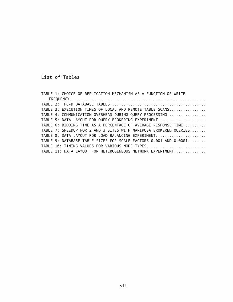
List of Tables

TABLE 1: CHOICE OF REPLICATION MECHANISM AS A FUNCTION OF WRITE FREQUENCY.. .TABLE 2: TPC-D DATABASE TABLES..................................................................................................TABLE 3: EXECUTION TIMES OF LOCAL AND REMOTE TABLE SCANS.......................................TABLE 4: COMMUNICATION OVERHEAD DURING QUERY PROCESSING.....................................TABLE 5: DATA LAYOUT FOR QUERY BROKERING EXPERIMENT................................................TABLE 6: BIDDING TIME AS A PERCENTAGE OF AVERAGE RESPONSE TIME.............................TABLE 7: SPEEDUP FOR 2 AND 3 SITES WITH MARIPOSA BROKERED QUERIES.........................TABLE 8: DATA LAYOUT FOR LOAD BALANCING EXPERIMENT..................................................TABLE 9: DATABASE TABLE SIZES FOR SCALE FACTORS 0.001 AND 0.0001...............................TABLE 10: TIMING VALUES FOR VARIOUS NODE TYPES................................................................TABLE 11: DATA LAYOUT FOR HETEROGENEOUS NETWORK EXPERIMENT.............................

vii

Acknowledgements

First and foremost, I would like to thank my advisor, Mike Stonebraker. I came to

Berkeley for the express purpose of working with Mike. I feel incredibly fortunate to

have had the opportunity to do so. His foresight and excellent taste in research topics

have been the biggest influences in my development as a graduate student. When I

would stray away from the main point, Mike unfailingly shepherded me back.

I would like to thank my partner, Jeff Oakes, who was there when we jointly made the

decision to go back to school, weathered the separation and financial hardship with me,

and made what seemed at the time a large sacrifice in moving out to California. I have

Jeff to thank for my application to Berkeley in the first place. If he hadn’t suggested I go

elsewhere for my PhD, we would never have discovered this wonderful place which we

now call home. I would also like to thank my parents. My mom and dad have always

placed education at the top of their list of priorities, and it was my mother’s saying “you

only get educated once” that prompted me to go back to graduate school in the first

place. Their bedrock of support, both financial and emotional, has given me the freedom

to pursue my dreams.

I would like to thank the rest of the Mariposa team, who spent long hours designing,

implementing, refining and debugging Mariposa: To Andrew MacBride, whom I had the

extreme good fortune to meet upon first arriving in California, for his excellence as a

software architect and good humor; To Paul Aoki, for his encyclopedic knowledge of

the code base, as well as database management systems in general. To Adam Sah, for his

lightning-quick mind and unceasing energy and optimism. To Marcel Kornacker, Rex

Winterbottom, Andrew Yu, Avi Pfeffer, who all contributed substantially to the

implementation effort. I would also like to thank Sunita Sarawagi and Allison Woodruff,

two of Mike’s other graduate students, for helping me get through prelims and quals and

always being around as sounding boards. Finally, I would like to thank Alice Ford,

Mike’s grants administrator, who not only made sure I didn’t starve, but was always up

for going and getting a cup of coffee.

viii

1IntroductionThis thesis describes query processing in the Mariposa distributed database management

system (D-DBMS). Mariposa is an example of an agoric system, in which distributed

resource management problems are expressed in economic terms. Each Mariposa site

can buy resources from, or sell resources to, other Mariposa sites. The designers of

Mariposa intended for the system to address the shortcomings of previous distributed

database management systems. The architecture of a traditional D-DBMS is described in

Section 1.1.1. Three implementations of D-DBMSs are described in Sections 1.1.1.2

through 1.1.1.4. First and foremost among the shortcomings of these systems is their

inability to scale to a large number of sites. As discussed in Section 1.1.1.1, the use of an

exhaustive, cost-based distributed query optimizer limits the number of sites to which

these systems can scale.

The Mariposa designers intended for a Mariposa system to be able to scale to thousands

of sites. In order to achieve this goal, they had to depart from the centralized approach to

processing site selection used in traditional distributed query optimizers. Instead of

ordering a remote site to perform work on its behalf, a Mariposa site may attempt to

contact the remote site first and acquire the necessary resources by purchasing them.

This approach dovetailed with the second goal for Mariposa: site autonomy. By

decentralizing the process of site selection, Mariposa not only achieves the potential to

scale, but also allows each site to manage its resources autonomously. As in a real

economy, a Mariposa site sells its resources to other sites, raising and lowering its prices

2

in order to maximize revenue. Using the simple mechanism of price, Mariposa can

address several other shortcomings of traditional D-DBMSs. These include:

1 Relative machine load: A distributed optimizer assigns processing sites to

different parts of the query plan, effectively allocating various amounts of

work to each processing site, while ignoring the current load at that site. This

can result in imbalances in the load of different machines. Evenly balancing

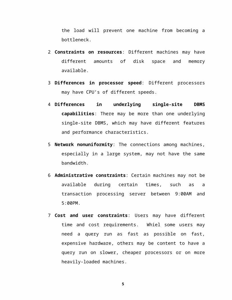
the load will prevent one machine from becoming a bottleneck.

2 Constraints on resources: Different machines may have different amounts of

disk space and memory available.

3 Differences in processor speed: Different processors may have CPU’s of

different speeds.

4 Differences in underlying single-site DBMS capabilities: There may be more

than one underlying single-site DBMS, which may have different features and

performance characteristics.

5 Network nonuniformity: The connections among machines, especially in a large

system, may not have the same bandwidth.

6 Administrative constraints: Certain machines may not be available during

certain times, such as a transaction processing server between 9:00AM and

5:00PM.

7 Cost and user constraints: Users may have different time and cost requirements.

Whiel some users may need a query run as fast as possible on fast, expensive

hardware, others may be content to have a query run on slower, cheaper

processors or on more heavily-loaded machines.

Of all of the factors listed above, only relative machine load has been a serious focus of

research. Work in the area of load balancing is described in Section 1.1.2. There has

3

been a small amount of research focusing on query processing under changing resource

availability. This work is described in Section 1.1.3.

As mentioned above, Mariposa is an agoric system. Agoric systems are a relatively

recent approach to distributed resource management. The underlying principles of agoric

systems and a few implementations of such systems are described in Section 1.1.4. The

Mariposa architecture is described in Section 2. I was responsible for the modules in

Mariposa which govern creating query plans, distributed query scheduling and

distributed query processing. These modules¾the fragmenter, the broker and the

bidder¾are described in detail in Sections 2.1.1.2 through 2.1.1.4.

As in a real economy, a Mariposa system uses price as a tool to effect changes in system-

wide behavior. Section 2.2 presents several pricing policies designed to address each of

the shortcomings of centralized D-DBMSs listed above. Section 3 presents experimental

results, beginning with some basic distributed performance characteristics and going on

to evaluate each of the pricing policies. Section 4 briefly presents some conclusions and

discusses directions for future work.

1.1Previous Work

1.1.1Distributed Database Management SystemsImplementations of relational database management systems (DBMSs) [STO76],

[ATS76] followed closely on the heels of the introduction of the relational model by E.F.

Codd in 1970 [CO70]. After the first relational DBMSs were implemented, it seemed a

natural extension to create systems that could access data stored at several sites connected

by a network. The first distributed relational database management systems, described in

4

this section, have the common characteristic of having been implemented in conjunction

with, or as a follow-on to, a single-site database management system. Because of the

existence of a more-or-less working single-site DBMS, the distributed database designers

took the sensible approach of layering the distributed portion of their systems on top of

the single-site systems they had available.

An example distributed database is shown in Figure 1. There are three database server

sites: Berkeley, CA; Fort Wayne, IN and Fairlee, VT. There are two tables: DEPT,

which stores department information, and EMP, which stores employee information.

The DEPT relation has two attributes: the department name and the department number.

The EMP relation contains the employee name, salary and the department number in

which the employee works. The EMP relation is stored at Berkeley and the DEPT

relation is stored at Fort Wayne.

Berkeley

Fort Wayne

Fairlee

EMP

DEPT

Name Salary DeptNoJeff 100K 1Adam 90K 1Drew 80K 2Dave 70K 3

Name NoEngineering 1Support 2Accounting 3

Figure 1: Example Database

5

A representative example of a distributed database architecture is shown in Figure 2. A

relational database query, expressed in a query language such as SQL, is entered by a

user via a frontend application, typically running on a client machine. The example

query shown in Figure 2 returns the average salary per department. The frontend

application passes the query to the distributed DBMS at a site that is part of the system.

This site is designated the master site for the query, since it will instruct other sites to

perform work. The other sites are called slaves. A slave site has no autonomy; it cannot

refuse to perform work when instructed to do so by a master site. Nor can a slave site

perform work that was not passed to it by the master site. The SQL query is first passed

into the parser, which checks the table and column references and syntax.

SELECT AVERAGE(EMP.SALARY), DEPT.NAMEFROM EMP, DEPTWHERE EMP.DEPTNO = DEPT.NOSORT BY DEPT.NAMEGROUP BY DEPT.NAME;

Frontend Application

Distributed DatabaseManagement System

Parser

Optimizer

Executor

SQL Query

Query Plan

Slave Site 1

Slave Site 2

Subplan

Subplan

Master Site

Figure 2: Traditional Distributed Database Management System Architecture

6

A common goal among designers of distributed DBMSs was location transparency. The

user was not aware where database tables were stored or which sites were involved in the

execution of the query. Location transparency was an extension of the declarative nature

of relational database management systems, in which a user simply specified the data he

or she wanted returned, but it was the job of the DBMS to figure out the best way to do

it. This is traditionally the job of the optimizer. The steps the DBMS will execute to

process a query is called a query plan. A query plan can be represented as a tree

composed of nodes and edges. Each node represents some indivisible operation, such as

a table scan, a sort, a join or an aggregate. The edges represent the flow of tuples from

one operator into another. Each node is executed at one site. Each node has an associated

cost, which is the value of the optimizer’s cost function for that node. This cost function

may include terms for CPU usage and disk accesses. A distributed DBMS generally adds

in the communication cost of sending intermediate results from one site to another as

well. The cost of a plan is the sum of the costs of its nodes. The optimizer’s job is to find

the query plan with the lowest total cost. Traditional distributed D-DBMSs performed

site selection inside the query optimizer. This made a distributed optimizer’s task much

more difficult. The number of potential processing sites for each node in the query plan

could be greater than one, effectively increasing the size of the solution space of query

plans exponentially.

The optimizer passes the query plan, complete with processing sites, to a distributed

executor, which proceeds to tell the remote sites to start processing by sending each one a

description of the work it is to perform. Each site involved in the distributed query

performs its task by passing it to the local single-site DBMS. The results of the single-

7

site query plan are then sent to the next processing site, which was determined by the

master site. The tuples in a single-site result may be materialized as a temporary relation

at the local site first and then sent in their entirety, or they may be streamed to the next

site as they are created. For the example query, a distributed optimizer may produce the

query plan shown in Figure 3. The DEPT relation is scanned at Fort Wayne and sent to

Berkeley where it is joined with the EMP relation. The result of the join is sorted, and

the average salary per department is calculated at Berkeley.

JOIN

SORT

AVERAGE

SCAN(DEPT)

SCAN(EMP)

Berkeley

Ft. Wayne

Figure 3: Query Plan for Example Query

1.1.1.1Scalability of Exhaustive Distributed Query OptimizationAn exhaustive distributed optimizer considers a subset of all query plans which calculate

the answer to a user’s query. The variables which the optimizer must consider are:

access methods (unindexed or indexed scans); join order, if there are multiple relations to

be joined; join methods; and the site at which each operation is to be performed. Some

operations, such as a relation access, can be performed at only a limited number of sites.

Other operations, such as joins, can be performed at any site. The size of the solution

space of distributed plans can be calculated as follows:

T number of base tables accessed in a query

8

Ai number of access methods available for table Ti

Nj number of nodes in query plan j

S number of processing sites

Each access method can be used without regard to the access methods used for the other

relations. Therefore, the number of combinations of access methods can be calculated as

b Aii

T

1

The number of different orders in which the tables can be accessed is equal to number of

permutations of b=b!. The number of single-site plans is equal to the number of join

orders. This is equal to the number of parenthesizations of b!, which can be calculated as

Jb

b

!

/!

43 2

Since each operation (with the exception of base table accesses) can be performed at any

site, the number of distributed plans is

N T

j

JjS

1

Implementations of exhaustive distributed query optimizers did not materialize every

plan in the solution space, but used a technique called branch and bound to limit the

number of plans considered [WD81]. However, this does not change the underlying

exponential growth of the solution space as the number of processing sites increases,

since it only decreases the value of the exponent Nj - T. For even a simple query plan,

such as the example query, the number of distributed plans grows quickly. For example,

9

assume that there are eight nodes per plan1 on average and that there is one index on each

of the two relations EMP and DEPT. If an optimizer could iterate through the entire plan

space for one site in one second, ten sites would take a week and a half and twenty sites

would take more than four million centuries. The number of sites that a distributed

database management system which uses exhaustive, cost-based optimization can

manage is therefore constrained by pushing the site selection into the optimizer.

The factors that can be considered when comparing distributed plans in traditional cost-

based optimizers must be limited, due to the explosive growth in the size of the solution

space. Given the same information about table sizes, selectivities and data placement, a

traditional optimizer will always produce the same distributed plan for a given query.

Therefore, traditional optimizers are inflexible, or static. However, there are many

factors in addition to those used in a cost-based optimizer’s cost function that can affect

query response time, as well as very practical considerations which have been ignored in

traditional distributed database management systems. As mentioned in Section 1, factors

that have a profound impact on query execution time include relative machine load,

changing resource availability, differences in processor speed, network nonuniformity,

administrative constraints, user constraints and cost constraints.

Designers of early D-DBMSs all more or less followed this blueprint when creating their

systems. There were some differences in their approaches to distributed query

optimization and execution. In the rest of this section, three distributed database

management systems are described: SDD-1, distributed INGRES and R*. Each

1 The example query could produce plans with 7, 8 or 9 nodes, depending on the number of index scans used in place of sequential scans followed by sort operations.

10

description begins with the genesis of the system, then briefly outlines its architecture.

Their approaches to query optimization and execution are compared and contrasted.

1.1.1.2SDD-1SDD-1 was the first general-purpose distributed DBMS developed. An overview of

SDD-1 is presented in [RB80]. The initial design was started by Computer Corporation

of America in 1977, the first release came a year later and a full release, including

distributed query processing, concurrency control and reliable distributed updates, a year

after that. Users interacted with SDD-1 via a high-level language called Datalanguage

[CC78]. Datalanguage was similar to the now-ubiquitous SQL, although it combined

SQL’s declarative style with procedural programming constructs. SDD-1 supported

distributed transactions and distributed query processing. SDD-1 also supported

fragmented storage of base relations. A database table in SDD-1 could be divided into

horizontal fragments, each of which contained a unique subset of tuples. The union of

the fragments was the entire table. Two fragments could be stored at two different sites.

The architecture of SDD-1 was divided into three completely separate virtual machines.

This design approach simplified the implementation of the system by dividing its

functional pieces along well-defined boundaries. The three virtual machines in SDD-1

were: Transaction Modules (TM’s), Data Modules (DM’s) and a Reliable Network

(RelNet). A data module was responsible for storing data at a single site and was, in

effect, a single-site database management system. A transaction module was responsible

for the distributed execution of a user query, and included support for access to base table

fragments, distributed concurrency control, distributed query optimization and distributed

query execution. The Reliable Network module connected the transaction modules and

11

the data modules together in a robust fashion. The reliable network provided guaranteed

delivery (even when the sender or receiver was down), transaction control, site

monitoring and a network clock.

The approach taken to query optimization and query processing in SDD-1 is presented in

[BER81]. The most important assumption made by the authors is that network

bandwidth was by far the most scarce computational resource. This assumption was

certainly true in the case of SDD-1, which was implemented on top of ARPANET. The

ARPANET had a sustained bandwidth of only 10kbps, which was two orders of

magnitude lower than the single site resources, CPU time and disk I/O [BER81]. This

assumption led to a simplified query optimization strategy: only count network cost in

the optimization process, and assume that all other processing comes for free.

SDD-1 was the first system to formalize the semi-join operation, wherein the join

attribute of one relation is used to restrict the number of tuples in the second relation

[BER81]. Referring to the example database, consider the query shown in Figure 4,

which returns the average salary for the engineering department.

SELECT AVERAGE(EMP.SALARY)FROM EMP, DEPTWHERE EMP.DEPTNO = DEPT.NO ANDDEPT.NAME = ‘ENGINEERING’;

Figure 4: Query to Return Average Salary for Engineering Department

A semi-join of EMP and DEPT that would restrict the size of EMP would be carried out

as shown in Figure 5. First the DEPT.no attribute would be projected from the DEPT

relation after the selection criteria had been applied. Then, the values of DEPT.no would

be compared to the values in EMP.deptno and any tuples that did not match a department

12

number would be eliminated. If EMP and DEPT were at different sites, this could

decrease the number of tuples from the EMP relation sent over the network. In the

example, half the tuples are eliminated from the EMP relation. In a situation such as that

faced by the developers of SDD-1, where the network is a bottleneck, semi-joins are

likely to be a good tradeoff, since they effectively increase usage of relatively cheap

single-site resources (additional disk I/O and CPU time) in an attempt to decrease the

relatively more expensive network traffic.

Berkeley

Fort Wayne

Fairlee

EMP

DEPT

Name Salary DeptNoJeff 100K 1Adam 90K 1Drew 80K 2Dave 70K 3

Name NoEngineering 1Support 2Accounting 3

DEPT.No = 1

Figure 5: Semi-Join between EMP and DEPT

Query optimization and query processing in SDD-1 took the form of moving all

necessary data to one “assembly site” and performing the query there. The goal of the

SDD-1 query optimizer was therefore to minimize the amount of data that was

transmitted to the assembly site. The optimizer started by following a basic “hill-

climbing” strategy and then applying two post-processing steps. The hill-climbing

13

strategy was a greedy algorithm which always chose the next cheapest operation to

perform. Because network communication was the only cost factor, the optimizer first

applied all single-site operations which would restrict the size of a relation, such as

selections, projections and semi-joins where both relations resided at the same site. After

all single-site operations had been applied, the SDD-1 optimizer considered all semi-

joins where the two relations were stored at different sites, and the one which was likely

to reduce the size of the database most was applied. This step was repeated until no

semi-joins could be found which would reduce the size of the database. When the query

was executed, all the single-site operations were processed first, then semi-joins where

the two relations were stored at different sites. The results which were materialized at

each site were sent to the assembly site.

The designers of SDD-1 were quick to point out that a greedy heuristic could not

guarantee an optimal query processing strategy, and so proposed two post-processing

steps which seemed reasonable. The first step was to permute the order of two semi-

joins when it would decrease the cost of one without increasing the cost of another. For

example, if relation A were used to decrease the size of relation B, and relation C were

used to decrease the size of relation A, then the semi-join involving C and A should

always be done first. Decreasing the size of A may make the semi-join between A and B

more effective in reducing the size of B. The second post-processing step was to prune

semi-joins rendered unprofitable by the choice of final assembly site. This step

effectively eliminated semi-joins in which the relation whose size would be restricted

resided at the assembly site. Since this relation would not be moved, restricting its size

would not save network utilization.

14

Although the designers and implementors of SDD-1 managed to create a working

prototype by 1979, SDD-1 was hobbled by its dependence on ARPANET. A network

which can slow down query processing by two orders of magnitude limits the practical

usefulness of a distributed DBMS. Faster kinds of networks were becoming available,

however. In other early distributed database management systems, namely R* and

distributed INGRES, it was shown that the network was not necessarily the main

bottleneck in query processing [SE80] and, indeed, that the elapsed time to solve a query

could often be reduced by increasing parallelization, which necessarily increased network

utilization [STO86]. The next section presents an overview of distributed INGRES,

which was not married to the ARPANET, and therefore had more flexibility in choosing

query processing strategies.

1.1.1.3Distributed INGRESDistributed INGRES [STO86] was spawned from the INGRES project [STO76] in 1977.

Distributed INGRES consisted of a process called master-INGRES, which ran at the site

where a user’s query originated, and a process called slave-INGRES, which ran at any

site where data needed to be accessed. The master process was a middleware layer that

parsed the query, performed view resolution, and optimized the query to produce a

distributed plan. The slave process was single-site INGRES with a few minor extensions

and the parser removed. In addition to these two basic components, there was a third

process, called the receptor, which was spawned by a slave to receive a relation that

needed to be moved from one site to another. A master process could instruct a slave

process to do exactly two things: perform a local query, and move a table to a subset of

other distributed INGRES sites. This led to a “step-wise” execution model wherein a

15

complex distributed query was broken down into a series of single-site queries. The

result of each such query was materialized into a temporary relation and then moved to

the next processing site. Since distributed INGRES supported fragmentation of base

tables, a temporary relation could reside at one or more sites. Furthermore, an operation

could be parallelized over an arbitrary number of sites. If the operation were a join, the

tuples of one relation were fragmented and distributed evenly among the processing sites,

while the other relation was sent to each site in its entirety.

Query optimization in distributed INGRES [EPS78] was an extension of the optimizer

used in single-site INGRES [STO76]. Both optimizers used query decomposition

[WON76] to arrive at a query plan. Query decomposition was a top-down technique that

reflected the step-wise execution model of INGRES. A complex query was iteratively

decomposed into components by using a greedy heuristic which always selected the next-

cheapest operation to perform. Joins were sorted in increasing order of expected join

result, and all predicates were pushed down the plan tree as far as possible. The two-way

join with the smallest expected result size was performed first, and each subsequent

relation was chosen to minimize the expected intermediate result size. This created a

left-deep plan tree, in which every inner relation was a base table, and every outer

relation but one was an intermediate join result.

In single-site INGRES, reducing a query to its components in this way resulted in a

complete, single-site query plan. In distributed INGRES, each component could be

scheduled at one or more sites, necessitating additional optimization. To assess the

relative goodness of the various possible strategies which could be used to compute each

16

component, the distributed INGRES designers proposed a cost function. The cost

function took into account the two factors deemed most likely to be important to users of

the system: total network utilization and distributed processing time. The cost function

had a term for each, and used constants to reflect their relative importance:

cost = C1 * network-communication + C2 * processing-time

The optimizer considered each component in isolation, selecting the strategy that would

minimize the cost function. Computing the network cost was relatively straightforward,

given the relation or relations to be moved and the number of receiver sites. The authors

assumed that relative elapsed time for different operations could be estimated with

enough accuracy for comparison. The designers presented an algorithm to minimize

network communication for each component, and an algorithm that would minimize the

elapsed time by maximizing parallelism.

Some performance results for distributed INGRES are reported in [STO83]. Distributed

INGRES was tested against single-site INGRES on a single local system to measure the

overhead due to extra processing. Then, distributed INGRES running on a remote site

was tested so that network overhead could be measured. Finally, distributed INGRES

was tested with two sites and again with three sites. The database tables, EMP and

DEPT, were distributed evenly among the sites. The EMP table was 114K in size and

had 30,000 tuples. The DEPT table was 27K in size and had 1,500 tuples. The first

experiment consisted of a series of single-tuple updates of the EMP table. The second

experiment retrieved all the tuples in the DEPT table. The third experiment performed a

natural join between the two tables.

17

Distributed INGRES on a single local machine was about twenty percent slower for

updates than local INGRES, but had comparable performance for read queries. When

update queries were run on a single remote site, they were an additional ten percent

slower than updates performed locally. Read queries performed remotely were slower by

about 30%. 32% of this slowdown was due to network overhead. Network bandwidth

was not considered to be a limiting factor as much as the additional overhead of setting

up and tearing down network connections.

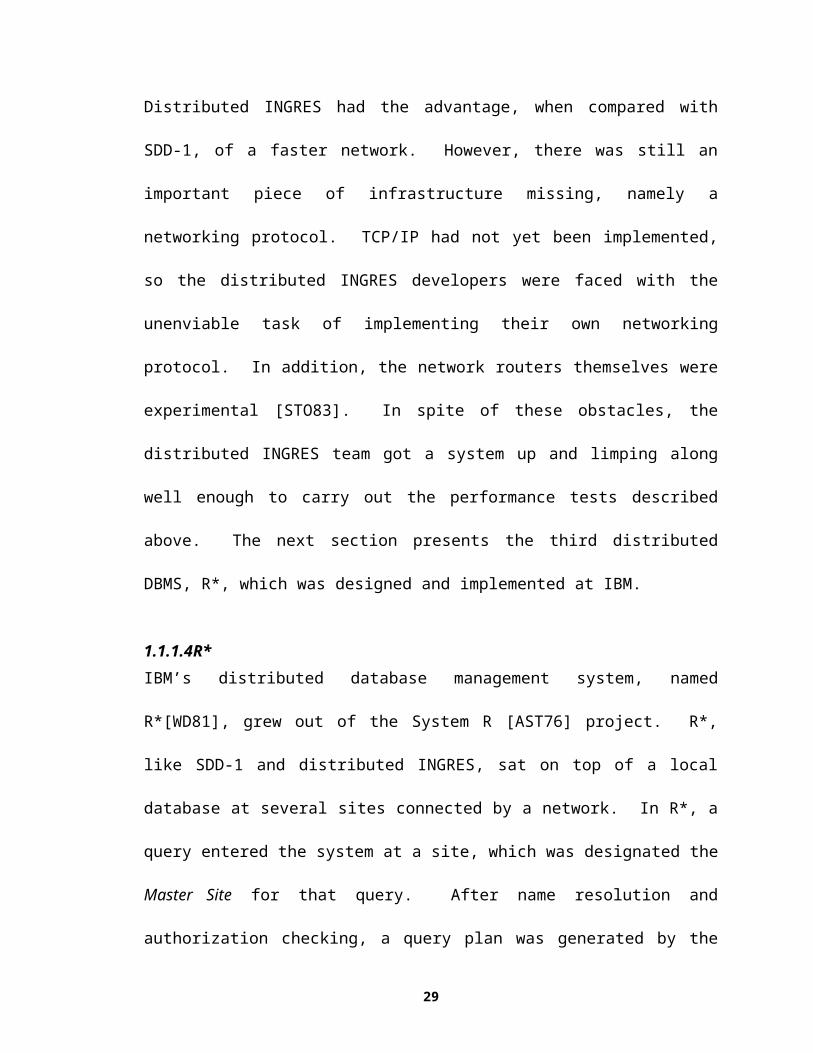
Distributed INGRES had the advantage, when compared with SDD-1, of a faster

network. However, there was still an important piece of infrastructure missing, namely a

networking protocol. TCP/IP had not yet been implemented, so the distributed INGRES

developers were faced with the unenviable task of implementing their own networking

protocol. In addition, the network routers themselves were experimental [STO83]. In

spite of these obstacles, the distributed INGRES team got a system up and limping along

well enough to carry out the performance tests described above. The next section

presents the third distributed DBMS, R*, which was designed and implemented at IBM.

1.1.1.4R*IBM’s distributed database management system, named R*[WD81], grew out of the

System R [AST76] project. R*, like SDD-1 and distributed INGRES, sat on top of a

local database at several sites connected by a network. In R*, a query entered the system

at a site, which was designated the Master Site for that query. After name resolution and

authorization checking, a query plan was generated by the optimizer, complete with

processing sites. Each site was sent its respective subplan to be executed. In contrast to

SDD-1 and distributed INGRES, which materialized intermediate results at slave sites, an

18

R* site would forward tuples to the next site in the global query plan as they were

created, first packaging them into network blocks to decrease per-tuple communication

overhead. Since an R* processing site may have had more up-to-date information about

local access methods, it could select different access paths than were indicated in the

subplan passed to it by the master site. R* sites had a degree of site autonomy, inasmuch

as sites were allowed to move tables, add and drop access paths, and fragment relations

without centralized control. Because the Master Site took responsibility for site

selection, if a site could not perform the work, for instance because a table had moved,

the slave site returned an error message to the Master Site and the plan was aborted, a

new plan generated, and the query started over.

The R* optimizer [WD81] used a bottom-up approach to optimization nearly identical to

the one used by its single-site predecessor, System R [AST76]. In this approach, the

optimizer considered the entire space of plans that would produce the right answer. The

plans were created “bottom up” by first enumerating all the single table accesses, then the

two-way joins, then three-way joins, etc. In order to compare plans to one another, R*

used a cost function, similar to that used in distributed INGRES. The R* cost function

was an extension of the single-site cost function used in System R. The System R

optimizer’s cost function considered only single-site resources, namely disk I/O and CPU

cost. The R* cost function, shown in Figure 6, included two terms to account for

network cost: a per-message cost and a per-byte cost.

TOTAL_COST = I/O_COST + CPU_COST + MESSAGE_COSTI/O_COST = I/O_WEIGHT * NUMBER_OF_PAGES_FETCHEDCPU_COST = CPU_WEIGHT * NUMBER_OF_CALLS_TO_RSSMESSAGE_COST = MESSAGE_WEIGHT * NUMBER_OF_MESSAGES_SENT +

BYTE_COST * NUMBER_OF_BYTES_SENT

19

Figure 6: R* Optimizer Cost Function

The R* designers had several advantages over the developers of SDD-1 and distributed

INGRES. First among these was the existence of a networking protocol, called VTAM,

on which they could base their communication. Secondly, the R* team benefited from

having a large number of well-trained programmers who had not only the experience of

System R to draw upon (as well as its code base) but also the lessons learned from SDD-

1 and distributed INGRES. As a result, the R* implementation was much more succesful

than the other two projects. The approach taken in designing the R* optimizer has the

advantage of considering the entire plan space, and so can be guaranteed to produce good

plans. The R* optimizer will therefore be used as a basis for comparison in the

experimental evaluation of Mariposa. The R* approach has a distinct disadvantage when

it comes to scalability and flexibility. Referring to the discussion in Section 1, using a

centralized exhaustive distributed query optimizer limits the scalability of an R* system

and prohibits consideration of factors such as load imbalance, changing resource

availability, etc. Of these factors, only relative machine load and changing resource

availability have led to serious research efforts. Research that addresses differences in

machine load has attempted to achieve load balancing, that is, to distribute the load as

evenly as possible across the available machines. Research focusing on disk and memory

constraints has delayed the selection of a query plan until run-time, when factors such as

memory and buffer availability can be taken into account. This approach is called

dynamic query optimization. The next two sections describe research in load balancing

and dynamic query optimization, respectively.

20

1.1.2Load Balancing in Parallel and Distributed Database Management SystemsLoad balancing has been a topic of research in both parallel and distributed database

management systems. Recall the example distributed query execution from Section 1.1.1

shown in Figure 3. All of the work was performed at Fort Wayne and Berkeley, while

the third site, Fairlee, was idle. If there were several such queries in the system at the

same time, the Fort Wayne and Berkeley sites would become overloaded and response

time would suffer. The goal of load balancing is to distribute the work being performed

as evenly as possible across the available machines so that system performance will

degrade more gracefully.

This section begins with a theoretical discussion of load balancing. In its simplest form,

load balancing is an NP-complete problem. Parallel and distributed query processing

environments present additional complications, which are described next. Parallel

database management systems have combined attempts at load balancing with attempts to

achieve optimal parallelism. This section continues with a discussion of load balancing

in parallel DBMSs in Section 1.1.2.2. The computational complexity of query

optimization and load balancing in distributed and parallel database management systems

has led to the two-phase approach, in which a query is optimized first using a single-site

optimizer, producing a single-site query plan which is then scheduled. The two-phase

approach was first introduced in the XPRS parallel database management system

[STO88], which is described next. This section continues with a description of

approximation algorithms which also used the two-phase approach . These algorithms

were designed to achieve load-balancing while maximizing pipelined parallelism.

21

Finally, a research effort designed to achieve load balancing in a distributed database

management system is discussed.

1.1.2.1Computational Complexity of Load BalancingIn the most general sense, the goal of load balancing is to take several jobs of varying

sizes and schedule them on a set of machines so that the load is as evenly distributed as

possible. Put another way, the goal of load balancing is to minimize the load on the most

heavily-loaded machine. This problem is also known as the multiprocessor scheduling

problem [GJ91]. The set-partition problem, which is known to be NP-complete [GJ91], is

a special case of the multiprocessor scheduling problem. The set-partition problem takes

as input a set of numbers and asks whether the set can be partitioned into two disjoint

subsets such that the sum of the elements of one equals the sum of the elements of the

other. If the multiprocessor scheduling problem is restricted to finding a solution in

which the load on all processors is equal and the number of processors is two, it is

analogous to the set-partition problem. Therefore, if we could solve the multiprocessor

scheduling problem, we could solve the set-partition problem. Therefore, multiprocessor

scheduling must be NP-complete.

There are two factors inherent in parallel and distributed DBMSs that further complicate

load balancing: blocking operators and data dependencies. Operators, represented as

nodes in a plan tree, can be separated into two types: blocking and pipelining. A

blocking operator is one which must finish receiving tuples from the operator(s) below it

before it starts to output tuples to its parent. An example of a blocking operator is the

sort operator. No output tuples are produced by a sort until all input tuples have been

processed. Conversely, a pipelining operator streams tuples out as it receives them,

22

performing some processing in between. An example of this type of operator is a merge-

join, which scans two relations in order of the join attribute, joining tuples with matching

attributes together. Output tuples are produced by a merge-join as input tuples are

processed. Breaking a query at blocking operators naturally divides the query plan into

strides [STO96]. Each stride must complete before the one above it can begin.

Figure 7 shows the query plan from Figure 3 divided into strides. Every operator within

a stride must finish processing before the next stride can begin. For example, the EMP

and DEPT tables must be scanned and sorted before the join operator can start. In order

to minimize execution of a plan that contains blocking operators, the plan must first be

broken into strides, and each stride treated as a separate multiprocessor scheduling

problem. By minimizing the execution time of each stride, the execution time of the

entire query plan is minimized.

EMP DEPTName Salary DeptNoJeff 100K 1Adam 90K 1Drew 80K 2Dave 70K 3

Name NoEngineering 1Support 2Accounting 3

JOIN

EMP.Salary EMP.DeptNo100K 190K 180K 270K 3

DEPT.NameEngineering

SupportAccounting

Engineering

EMP.Salary

100K90K80K

DEPT.Name

Engineering

SupportEngineering

70K Accounting

SORT

AVERAGE

AVERAGE(Salary)

95K80K

DEPT.Name

EngineeringSupport

70K Accounting

Stride 1

Stride 2

Figure 7: Query Plan Divided into Strides

23

Data dependencies present a more difficult complication to multiprocessor scheduling. A

data dependency exists during the execution of a distributed plan when a table (either a

temporary table or a base table) is materialized at a site. The next operation in the query

plan cannot be executed at a different site without incurring communication cost. The

multiprocessor scheduling problem assumes that each job has a fixed cost. However,

because of data dependencies, the cost of a job will change depending on which

processor executes it; if it is executed at the site where its predecessor was executed,

there will be communication cost. Otherwise, network delay and communication

overhead at both the sender and receiver will be incurred.

1.1.2.2Load Balancing in Parallel Database Management SystemsResearch in parallel database management systems has focused on speeding up single

queries or single operators by exploiting intra-operator parallelism. In intra-operator

parallelism, an operation which can be performed in parallel by several processors at

once, such as sorting [DNS91] or hash joins [ZG90] is divided among all available

processors. An overview and discussion of intra-operator parallelism can be found in

[MD95]. Intra-operator parallelism attempts to solve the multiprocessor scheduling

problem by distributing the data as evenly as possible among the available processors,

that is, by avoiding data skew. Since each processor is performing the same task over

different data, it is important that the division of data among the processors be as close to

even as possible to achieve a balanced processor load. Overcoming data skew has been

studied extensively and the various approaches are well-documented in the literature

[WDJ91] [WDY91] [DNS92] [HLY93]. Since each operator is performed by all (or

several) processors, the problems of blocking operators and data dependencies disappear.

24

Because all of the processors are involved, they will all block. In a query in which all of

the operators are parallelized, the intermediate results of some operators will need to be

redistributed among the processors. This is the only communication overhead that is

incurred, and it is shared by all the processors.

A general treatment of the problem of query scheduling in parallel database management

systems is presented in [GI97]. The authors address intra-operator parallelism as well as

independent and pipelined parallelism. Independent parallelism occurs when two disjoint

subplans of a query plan are executed on different processors. Pipelined parallelism

occurs when a pipelining operator and its parent operator are executed on different

processors. As each tuple is produced by the first operator, it is pipelined to the second

one. [GJ91] presents two approximation algorithms for scheduling a query in a parallel,

shared-nothing environment. A parallel, shared-nothing environment typically consists

of independent machines connected by a local-area network. The algorithms work under

the assumption that each operator is going to utilize intra-operator parallelism and each

will be partitioned differently, so each operator always includes communication

overhead.

1.1.2.2.1The XPRS Parallel Database Management SystemA common approach to load balancing in distributed and parallel DBMSs is to optimize a

query as if there were only one processor, producing a single-site plan, and then to divide

the plan into parts and schedule the parts [HW93] [HAS95] [CL86]. The XPRS parallel

database management system [STO88], [HS93] used the two-phase optimization

approach. In XPRS, a query is first optimized using a System-R style single-site,

exhaustive, cost-based optimizer [SEL79]. The cost function used in the single-site

25

optimizer combines resource consumption and response time. The relative value of these

two factors is determined by a weighting factor. The plan tree produced by the optimizer

is then divided up into plan fragments by breaking the plan at its blocking nodes. After a

plan is broken up into fragments, each operator in a fragment is parallelized and the

fragment is passed to a parallel executor, which schedules the parallel components on the

available processors. The system was designed to be used on a shared-everything

(shared-memory and shared-disk) environment. [HS93] introduces the 2-Phase

Hypothesis, which states that, in a shared-everything environment, where only intra-

operator parallelism is used, the best parallel plan is a parallelization of the best

sequential plan.

[HS93] presents experimental results which support the 2-Phase Hypothesis, producing

parallelizations of every possible sequential plan and comparing them. The queries were

from the Wisconsin Benchmark [BIT83] plus a random benchmark, made up of multi-

way joins where the join clauses were generated randomly. The Wisconsin Benchmark

contains single-table scans and up to two-way joins. The plans were compared by filling

in their actual resource consumption and elapsed time into the cost function and

comparing the values. The experimental results in [HS93] suggest that, in general, the

hypothesis is true: the best sequential plan led to a suboptimal parallel plan in fewer than

0.006 percent of the queries when the cost function weighted resource consumption more

heavily. When response time was weighted more heavily, the error rate grew to around

eight percent as queries became more complex. This highlights an important point:

predicting resource consumption is relatively easy, but predicting response time, even

when a query is run in isolation, is far more difficult.

26

1.1.2.2.2Approximation Heuristics for Load Balancing and Pipelined ParallelismSince dividing a plan into parts and scheduling the parts in an optimal way is an NP-

complete problem, one approach to a solution is to use an approximation algorithm that

is guaranteed to produce a solution within some constant factor of optimal. [CHM95]

presents two approximation algorithms for dividing query plans into subplans for

scheduling on a parallel machine. The algorithms do not address intra-operator

parallelism, but instead focus on pipelined parallelism. They take as input a query plan,

represented as a directed acyclic graph. The nodes represent single-site operations and

the edges represent communication between sites. The algorithms first eliminate any

worthless edges. A worthless edge represents communication between two processors

that will always increase processing time. Nodes connected by worthless edges should

always be processed at the same site. Then, the algorithms artificially increase the

communication cost of each edge and eliminate any newly-created worthless edges.

Remaining edges represent communication between nodes which will be processed at

different sites. The nodes are scheduled using the LPT (Largest Processing Time)

algorithm [GRA69]. This is a greedy approximation scheme which sorts the subplans in

descending order of expected execution time and then assigns the largest subplan to the

least-loaded processor until all the subplans are scheduled. The LPT algorithm gives a

solution within 4/3 - 1/3n of optimal [GRA69], where n is the number of processing

sites. The algorithms presented in [CHM95] make several assumptions:

· The original query plans must consist only of non-blocking operators such as

sorts and hash table builds

· Processors are homogeneous

27

· Network latency is zero

· The execution time of a single node can be predicted accurately

· There are no data dependencies

1.1.2.3Load Balancing in a Distributed Database Management SystemThe two-phase approach was used to create distributed query plans in a multi-user

distributed database environment in [CL86]. After a single-site query plan was

produced, it was broken up into query units. A query unit was the largest subplan of the

query plan that accessed only one relation. The query units were scheduled using the

following algorithm, named “LBQP” for “Load-Balanced Query Processing”: the

algorithm selected the query unit with the smallest number of potential processing sites,

which [CL86] called its “assignment flexibility”. This work assumed that there were

multiple copies of each relation, and therefore multiple sites at which a query unit could

be processed. Each query unit was assigned to the site with the smallest load, and the

process was repeated until there were no more query units to schedule. The algorithm

then carried out two post-processing steps, which were meant to minimize the overall

communication cost of the plan, and then assigned sites to the join operators, also by

minimizing communication cost.

The LBQP algorithm was compared to a static algorithm and two random algorithms

using a simulator. The static algorithm assigned each query unit to a predetermined site,

as if there were exactly one copy of each table. The first random algorithm, RANDOMf,

was for fully replicated data and simply ran a query in its entirety at a remote site. The

second random algorithm, RANDOMp , attempted to run each query unit at the site of its

28

predecessor. If this was not possible, a site was chosen at random from among the sites

where the table associated with the query unit resided.

In the experimental setup, a multi-user workload was simulated by varying the interval

between queries, or “think time” at each of the terminals in the distributed system. The

queries consisted of single-table scans, two- and three-way joins. The sizes of the three

relations, R1, R2 and R3, were twenty, five and five pages, respectively, corresponding

to 160K, 40K and 40K for 8K disk pages. The average response time per query was

measured. There were three different experimental scenarios, each designed to analyze

the effect of a different factor on query response time, as well as to see how the LBQP

algorithm fared.

The first experiment varied the number of sites at which a table was replicated. Both of

these experiments ran the same query repeatedly. When every table was replicated at

every site, the static algorithm outperformed the LBQP algorithm when system load was

high, but the LBQP algorithm performed better as system load decreased. The

RANDOMf algorithm performed worse than both algorithms for all levels of system

load. When the number of sites per table was reduced, the LBQP algorithm

outperformed both the static and the random algorithms for all system loads. As the

number of copies decreased, however, the random algorithm continued to perform better.

Under the heaviest workload and fewest copies, the random algorithm performs

comparably to the LBQP algorithm.

The second experiment varied the workload at each site by assigning each site a different

think time. The relations were fully replicated, meaning that each query could be run in

29

its entirety at any of the sites. With unevenly loaded sites, the LBQP algorithm

outperformed the other two algorithms by around twenty-five percent. The third

experiment varied the query type. In this experiment, fifty percent of the queries

referenced one table, thirty percent were two-way joins and the remaining twenty percent

were three-way joins. This experiment was performed with all tables fully replicated,

and again with one copies at four of the six processing sites. The experimental results

were similar to the first experiment, with LBQP outperforming the other two algorithms.

A few of the results in [CL86] are somewhat counterintuitive. First is that a random

algorithm performed poorly compared to a static algorithm. The static algorithm must

have achieved load balancing by selecting a different default site for each relation. Even

so, in a multi-user workload, a random algorithm should have distributed the load evenly.

With few copies and relatively high system load, the random algorithm performed

comparably to LBQP, indicating that the random algorithm may have outperformed

LBQP for one copy under heavy load. Compare the results obtained here with the

practical experience of transaction processing monitors [GRA93]. Transaction

processing monitors perform distributed load balancing as well other services. When a

request arrives from a client, the TP monitor decides whether to execute the request

immediately, queue it to run as soon as a server process becomes available, or send it to a

remote node for execution. Because TP monitors were designed for systems that process

many small transactions, the decision must be made quickly. Most TP monitors utilize a

few simple heuristics, such as round-robin or random assignment of work to processors.

30

Load balancing attempts to adapt distributed or parallel query processing strategies as

conditions between machines change and some resources become more available while

other are less so. The next section presents work in dynamic query optimization, which

also addresses the problem of changing resource availability.

1.1.3Dynamic Query OptimizationAs resources such as memory and disk space become more or less available, the query

execution strategy that will result in the lowest execution time changes. For example, a

hash-join may require 10MB of memory to create its hash table and keep it resident in

main memory. If there is 10MB of memory available, then this may be the optimal

strategy. However, if there is not enough main memory to keep the hash table resident, a

different join strategy, such as nested-loop or merge-join may be faster. There have been

a number of research efforts which address the problem of adapting to changing resource

availability. In contrast to research efforts in load balancing, which use heuristics to

produce query plans on the fly, research in this area has taken a more preemptive

approach.

The idea of dynamic query evaluation plans was introduced in [GW89]. In this strategy,

a query is optimized to produce a join order and place aggregates and selection

predicates, resulting in a query tree in which the exact operator methods are not

specified. For example, a base table selection does not specify whether an unindexed or

indexed scan should be used, nor does a join specify the join method. The operator

method selection is delayed until query execution, at which time a decision procedure is

run to determine and assign methods. In [GW89] a comparison of query strategies is

presented to show the potential benefits of late binding of methods. A two-way join was

31

executed with varying base table selectivities and therefore varying result cardinalities.

For result sizes of one tuple, using an index scan was found to be superior to a complete

table scan by a factor of ten. For result sizes of the same size as the base relations, index

scans were found to be worse by a factor of three.

[GW89] was an early paper and provided justification for more dynamic and flexible

query optimization strategies. The experimental results were not presented in the light of

changing resource availability, but rather as a solution to running queries that accept

user-defined query parameters. The solution proposed by the authors, namely late

binding of operator methods, does not allow selection among completely different query

plans, for example, those with different join orders. The authors acknowledge this as a

shortcoming.

A more complete and mature presentation of dynamic query evaluation plans is in

[CG94]. Instead of creating a query plan when a query is submitted, the authors pre-

compile a “super-plan”. These super-plans are created bottom-up, like the R* optimizer,

and contain all potentially good plans, depending on resource availability. When

comparing two alternative subplans during this pre-compilation phase, the optimizer

assigns a range of costs to each subplan reflecting the range of potential resource

availability. If the cost ranges overlap, then both subplans are included in the super-plan

with a choose-plan node above them. A choose-plan node may have several subplans

below it. At query execution time, the final plan is chosen by selecting the correct plan

below each choose-plan node, based on current resource availability.

32

The parameterized query optimizer presented in [IOA92] addresses the problem of

adapting to changes in the availability of computational resources in a manner similar to

[CG94]. Instead of creating a super plan containing all potentially good plans, a

parameterized query optimizer pre-compiles a query with a set of parameters describing

the resources available. Parameters are varied randomly, producing a set of

parameterized plans for each query. When a query is submitted, resource availability is

checked and the appropriate plan is selected.

The XPRS shared-nothing parallel database management system also addressed the issue

of resource availability at run-time [HS93]. The only resource addressed was buffer

space. The assumption was made that there would always be enough buffer space for a

hash-join. This led to a second hypothesis, in addition to the 2-Phase Hypothesis; The

Buffer Size Independent Hypothesis stated that the choice of the best sequential plan is

insensitive to the amount of buffer space available as long as the buffer size is above the

hashjoin threshold. There are two exceptions to this hypothesis: The cost of an

unclustered scan decreases sharply as available buffer space increases, while the cost of

an unindexed table scan remains constant. Secondly, the cost of a nested-loop join with

an index on the inner relation decreases as available buffer space increases, while the cost

of a hash-join remains relatively constant for buffer sizes above the hash-join threshold.

XPRS deals with this situation by inserting choose nodes in the query plan, similar to

[CG94].

All of the work done to date in dynamic query optimization has focused on single-site

DBMSs. The solutions have not been generalized to distributed DBMSs. Dynamic

33

query optimization and load balancing are more closely related to each other than may be

apparent at first glance. The goal of the two approaches is the same¾to reduce execution

time by altering query processing strategies to fit current resource availability. However,

there is a fundamental difference in their approaches. Whereas research in load

balancing has focused on heuristic solutions which generate a plan on-the-fly, work in

dynamic query optimization has taken the approach of enumerating all possible good

plans and then choosing one.

This approach does not address the exponential growth of the solution space in a

distributed system. The work described in [GW89], [CG94] and [IOA92] only addressed

one resource¾available memory¾and was restricted to single-site systems. Even so, the

super-plans in [CG94] can have more than five orders of magnitude more nodes in them

than a plan created on the fly. The number of parameterized plans that would have to be

generated in [IOA92] to provide a reasonable sample of all combinations of table layout,

buffer space, CPU usage, network usage and disk traffic is potentially enormous. Any

attempt at extending dynamic query optimization to distributed systems would run up

against exponential growth in the number of distributed plans, as is the case with a

distributed optimizer.

Load balancing and changing availability of resources are only a few of the factors

affecting the execution of a query, as mentioned in Section 1. All of the systems

mentioned so far have one thing in common: centralized control. The site where a query

originates is completely responsible for creating an execution strategy for the query. The

next section presents an overview of work focusing on a different approach to distributed

34

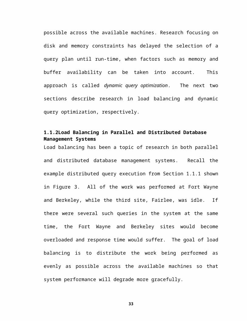
systems, called agoric systems, in which the resource allocation process itself is

distributed.

1.1.4Agoric SystemsA unifying theme in computer science, particularly in database management systems,

operating systems, programming languages and networks, is the management of

resources and coordination of action in large, complex systems. This is also true of

human society at large. However, society has had millennia to evolve customs,

institutions, laws, etc. to achieve these goals. The study of these systems has led to the

science of economics. As the Nobel Laureate F. A. Hayek observed in 1937:

...the spontaneous interaction of a number of people, each possessing only bits of knowledge, brings about a state of affairs in which prices correspond to costs, etc., and which could be brought about by deliberate direction only by somebody who possessed the combined knowledge of all those individuals... the empirical observation that prices do tend to correspond to costs was the beginning of our science.

[HAY37]

In other words, even though there is no one individual or institution in control, economic

systems “work.” Economists have studied the consequences of pursuing goals within

boundaries of limited resources and limited knowledge. There are parallels in computer

science, most notably in programming languages. In the early days of computing,

programs were relatively simple. They had few problems of coordination and the

complexity of a program could be grasped by a single mind. As programs became more

complex, bugs would appear because one module of a program would produce an

execution state that was inconsistent with the successful execution of another part.

Object-oriented languages [GR83], [CO86] addressed the problem of increasing

35

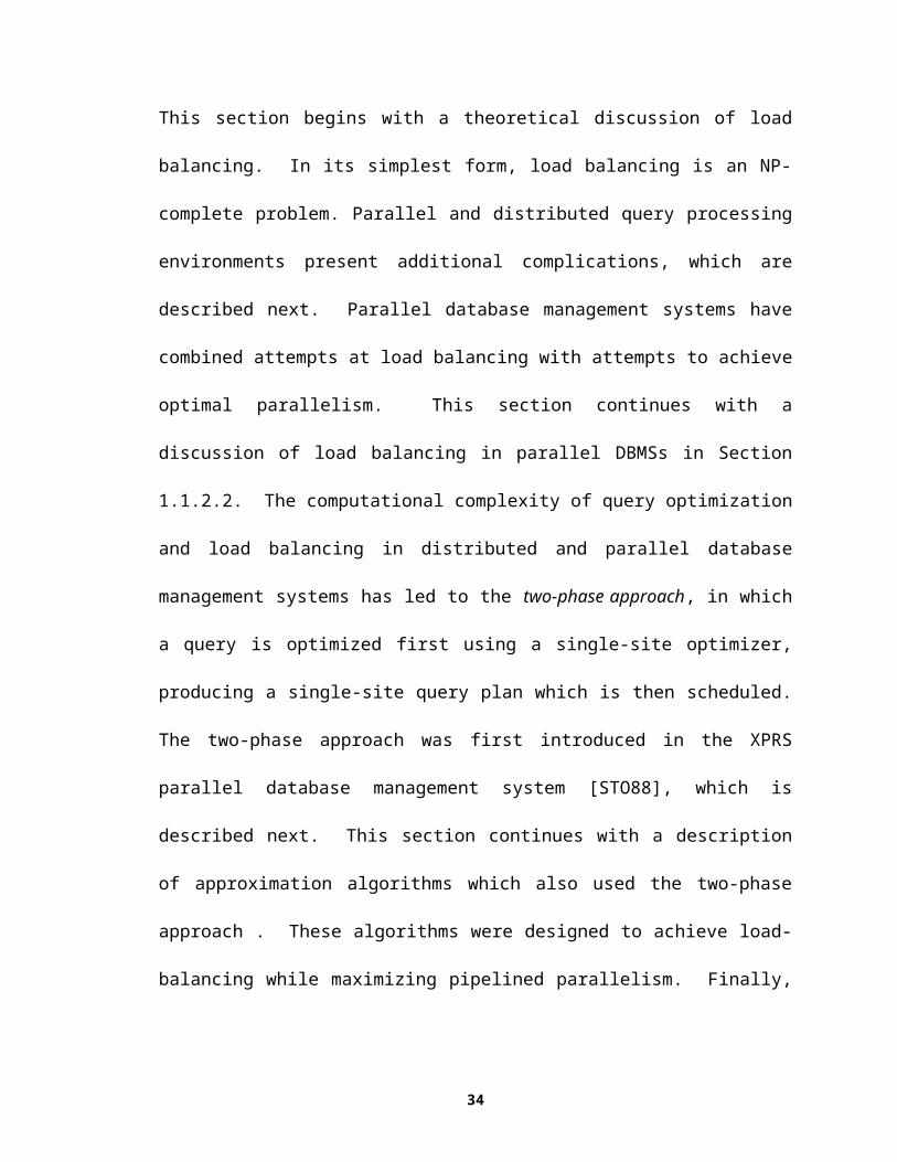
complexity by encapsulating an object’s behavior. The designers of object-oriented

languages realized the benefit of providing an environment in which each object had a

known and limited set of parameters within which it could decide its actions, thereby

making the programmer’s task much easier. Economists observed a similar

phenomenon:

The rationale of securing to each individual a known range within which he can decide on his actions is to enable him to make the fullest use of his knowledge...The law tells him what facts he may count on and thereby extends the range within which he can predict the consequences of his actions.

[HAY60]

While object-oriented programming languages have adopted a decentralized approach to

coordination, researchers in operating systems and database management systems have

taken a centralized approach to the problem of resource management. This approach

seems inherently rational and easier to understand than one in which the decision-making

process is distributed among autonomous agents. Likewise, a command economy, or

central planning (à la the former Soviet Union) has frequently been considered more

“rational”, since it involves the application of reason and logic to the economic problem.

However:

36

This viewpoint...smacks of the creationist fallacy¾it assumes that a coherent result requires a guiding plan. In actuality, decentralized planning is potentially more rational, since it involves more minds taking into account more total information. Further, economic theory shows how coherent, efficient, global results routinely emerge from local market interactions.

[MIL88]

The term agoric system, from the Greek word agora, meaning marketplace, was first

used by Mark Miller and K. Eric Drexler in [MIL88] to describe software systems

deploying market mechanisms for resource allocation among independent objects. An

agoric system is “a software system using market mechanisms, based on foundations that

provide for the encapsulation and communication of information, access and resources

among objects.” [MIL88] Each object is held accountable for the cost of its activity.

Providing for transfer of resources enables objects to buy and sell them. The resources

of a computational object, such as CPU time, disk space, disk I/O bandwidth and

network bandwidth are owned by that object. A consumer of these resources ultimately

must pay for them. If the consumer is also the owner, then currency simply flows within

the system, providing information which helps coordinate computational activities.

Agoric systems cast resource allocation problems in terms of economics. The programs

become buyers and sellers of resources, much like a real-life marketplace. As in a real

capitalist economy, buyers compete against one another for scarce resources and try to

get the best price they can, while sellers attempt to maximize their profit.

In a human economy, price mechanisms provide the “incentive” for behavior. The price

of something reflects how much it is valued by the system as a whole. To increase value,

a producer need only ensure that the price of its product exceeds the prices of the

37

resources consumed. The simple, local action of setting a price gains its power from the

ability of market prices to summarize global information about relative values. As F. A.

Hayek observed:

...the whole reason for employing the price mechanism is to tell individuals that what they are doing, or can do, has for some reason for which they are not responsible become less or more demanded....The term “incentives” is often used in this connection with somewhat misleading connotations, as if the main problem were to induce people to exert themselves sufficiently. However, the chief guidance which prices offer is not so much how to act, but what to do.

[HAY78]

In an agoric system, when there is a piece of work to be performed, the process in which

the work originated becomes a buyer. The buyer attempts to acquire the necessary

resources to perform the work by contacting a broker. The broker matches the buyer

with sellers, who have resources available. The buyer may communicate to the broker its

requirements regarding cost, time, etc. The broker attempts to find one or more sellers

who can meet the buyer’s requirements. If the broker succeeds, the buyer and sellers

enter into a contract. The sellers provide the goods and/or services they have agreed to,

and the buyer pays them the price agreed upon. As in real economic systems, price is the

mechanism by which a seller of resources responds to changing circumstances. A price

is set based only on information local to the seller, such as how much business it

currently has or how much business it has lost recently. As the behavior of individual

sellers is influenced by reaction from the rest of the economic system, the behavior of the

system as a whole changes.

38

1.1.4.1Implementations of Agoric SystemsCurrently, there are only a few systems documented in the literature that incorporate

microeconomic approaches to resource sharing problems. [HUBE88] contains a

collection of articles that cover the underlying principles and explore the behavior of

those systems. None of the agoric systems created to date explore the ability of pricing

to effect system-wide behavior based on incomplete local information. A brief

description of some implementations of agoric systems is described below.

[MAL88] describes the implementation of a process migration facility for a pool of

workstations connected through a LAN. In this system, a client broadcasts a request for

bids that includes a task description. The servers willing to process that task return an

estimated completion time and the client picks the best bid. The time estimate is

computed on the basis of processor speed, current system load, a normalized runtime of

the task and the number and length of files to be loaded. The latter two parameters are

supplied by the task description. No prices are charged for processing services. Although

this approach is described as “market-like” it doesn’t explore the nature of markets and

pricing; A client has complete knowledge of the state of the world and makes a decision

based on this global information.

Two systems, presented in [WAL92] and [DAV95] use a competitive bidding approach

to achieve fairness in resource distribution. A distributed process scheduling system is

presented in [WAL92]. In this system, CPU time on remote machines is auctioned off by

each machine and applications hand in bids for time slices. An application is structured

into manager and worker modules. The worker modules perform the application

processing and several of them can execute in parallel. The managers are responsible for

39

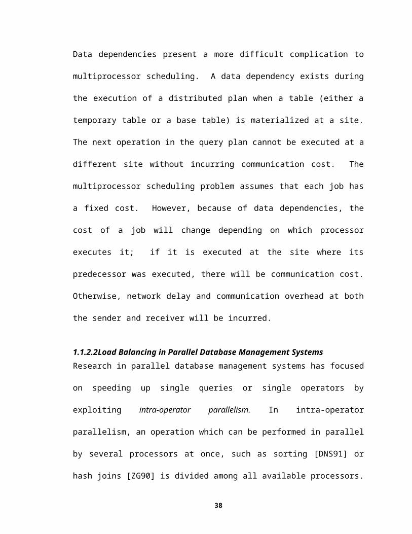
funding their workers and divide the available funds between them in an application-

specific way. Workers exchange their funds for CPU time. To adjust the degree of

parallelism to the availability of idle CPUs, the manager changes the funding of

individual workers. In [DAV95], the problem of multiple query management in a single-

site database is addressed by utilizing a resource broker, which sells resources to

competing operators. Both of these systems utilize competition and bidding to allocate

resources, however prices are fixed. It is the bids that are allowed to rise as a consumer’s

need increases. These systems are more closely related to auctions than to a market

economy.

In [FER93], a system in which fragments can be moved and replicated between the nodes

of a network of computers is presented. Transactions, consisting of simple read/write

requests for fragments, are given a budget when entering the system. Accesses to

fragments are purchased from the sites offering them at the desired price/quality ratio.

Sites attempt to maximize their revenue and therefore lease fragments or their copies if

the access history for that fragment suggests that this will be profitable. The relevant

prices are published at every site in catalogs that can be updated at any time to reflect

current demand and system load. The network distance to the site offering the fragment

access service is included in the price quote to give a quality-of-service indication. This

system does not explore the impacts on system-wide behavior of local decision-making;

every site needs to have perfect information about the prices of fragment accesses at

every other site, requiring global updates of pricing information. The name service is

provided at no cost and hence is excluded from the economy. Global updates of metadata

40

would likely suffer from a scalability problem, sacrificing the advantages of the

decentralized nature of microeconomic decisions.

When computer centers were the main source of computing power, several authors

studied the economics of such centers' services. The work focused on the cost of the

services, the required scale of the center given user needs, the cost of user delays, and the

pricing structure. Several results are reported in the literature, in both computer and

management sciences. In particular, [MEN85] proposes a microeconomic model for

studies of queuing effects of popular pricing policies, typically not considering the

delays. The model shows that when delay cost is taken into account, a low utilization

ratio of the center is often optimal. The model is refined in [DEW90]. The authors

assume a nonlinear delay cost structure, and present necessary and sufficient conditions

for the optimality of pricing rules that charge out service resources at their marginal

capacity cost. Although these and similar results were intended for human decision

making, many apply to agoric systems as well.

The next section describes Mariposa, an agoric distributed database management system.

Mariposa is a radical departure from existing distributed database management systems.

Mariposa describes the problems of distributed query processing, load balancing,

resource availability, copy management, etc. in terms of economics [STO96]. Recall

from Section 1 the shortcomings in traditional DDBMSs which Mariposa was intended to

address: scalability, load imbalance, resource constraints, nonuniformity of machines

and networks, administrative constraints, cost constraints and user constraints. In an

agoric system, buyers and sellers are completely autonomous and interact in a well-

41

defined, simple, loosely-coupled manner: buyers may contact whichever sellers they

choose, while each seller can set its prices as it sees fit. This natural site autonomy leads

to a system design which is inherently scalable. Furthermore, by allowing prices to

reflect changing resource availability, Mariposa should be able to address the problems

of load imbalance, resource constraints, etc. in a natural and intuitive fashion.

42

2MariposaIn the previous section, the limitations of traditional approaches to query optimization

and query processing in distributed database management systems were described. All of

these systems relied on a centralized approach to decision-making, and were therefore

limited in their scalability. Agoric systems represent a new approach to distributed

resource allocation based on economic principles. In agoric systems, independent sellers

set prices based only on local information and a manageable set of rules. In this section,

the Mariposa distributed database management system is described. Mariposa is an

agoric system and follows the guidelines for such systems presented in [MIL88].

The Mariposa project began in 1993 and, like the distributed DBMS projects described in

Section 1.1.1, followed on the heels of a single-site DBMS research project, in this case

Postgres [STO91]. The designers of the system had several goals which they intended

for Mariposa to achieve. In addition to overcoming the limitations of earlier distributed

database management systems, the designers intended for Mariposa to support for data

fragmentation, copies, lightweight data movement and distributed transactions. The

agoric approach was adopted to address the issue of scalability. The research challenge

was to achieve the other goals within the context of an agoric system.

This chapter begins with an overview of the Mariposa architecture, paying particular

attention to those modules for which I was directly responsible. These include the

fragmenter, query broker and bidder modules, which I designed and implemented.

Mariposa name service and the Mariposa copy system are also described in some detail.

43

I contributed significantly to the design and helped with the implementation of name

service and the copy system.

2.1The Mariposa ArchitectureA Mariposa system composed of three sites is shown in Figure 8. Like other distributed

DBMSs, Mariposa is middleware; that is, it is intended to be installed between a single-

site database management system and a frontend application. Several such installations

constitute a Mariposa economy. In a Mariposa system, the user submits a query and a bid

curve via a frontend application at a Mariposa site. In Figure 8, the query is entered at

Berkeley. This site is designated the home site for that query. The home site is simply

the site at which the query originated, and can be any Mariposa site.

Berkeley

Fort Wayne

Fairlee

SELECT AVERAGE(EMP.SALARY), DEPT.NAMEFROM EMP, DEPTWHERE EMP.DEPTNO = DEPT.NOSORT BY DEPT.NAMEGROUP BY DEPT.NAME;

Frontend Application

Mariposa Middleware

Parser

Optimizer

Fragmenter

SQL Query

Query Plan

Home Site

Query Broker

Fragmented Query Plan

Completed Query Plan

Coordinator

Bidder

EMP DEPTName Salary DeptNoJeff 100K 1Adam 90K 1Drew 80K 2Dave 70K 3

Name NoEngineering 1Support 2Accounting 3

EMP.Salary EMP.De ptNo100K 190K 180K 270K 3

DEPT.NameEngineeringSupportAccountingEngineering

EMP.Salary

100K90K80K

DEPT.Name

EngineeringSupportEngineering

70K Accounting

AVERAGE(Salary)95K80K

DEPT.NameEngineeringSupport

70K Accounting

Bid Curve

$

TIME

Bidder

Bidder

SingleSite

DBMS

SingleSite

DBMS

SingleSite

DBMS

Figure 8: Mariposa Architecture

44

The bid curve has cost on the y axis and time on the x axis. The bid curve allows the

user to communicate his or her performance and cost requirements to the system

succinctly by specifying how much the user is willing to spend to have a query processed

within a given amount of time. For example, if a user needs an answer quickly and has

no use for an answer after five minutes, he might use the bid curve shown on the left in

Figure 9. If a user doesn’t care when the answer comes back but wants to minimize cost,

she might use the bid curve on the right in Figure 9.

$

TIME

$

TIME0 5 0 5

Figure 9: Bid Curves

The query passes through a parser and an optimizer and is turned into a query plan. In

order to parse and optimize a query, the parser and optimizer need access to system

catalogs, or metadata. Mariposa name servers provide system metadata including type

information, data fragmentation and placement and statistics such as table size. Name

service in Mariposa is described in Section 2.1.1.1.3. To address the exponential growth

of the size of the solution space of distributed plans, Mariposa uses a single-site

optimizer, which produces a plan that minimizes single-site resource utilization. This is

the same approach taken in [HW93] [HAS95] [CL86]. Mariposa thereby determines the

join order and access methods, producing a query plan without the processing sites filled

in.

45

The query plan produced by the optimizer is passed into the fragmenter. The fragmenter

alters the single-site plan to reflect the underlying data fragmentation. The fragmenter is

further described in Section 2.1.1.2. The fragmented plan is passed into the query

broker, which operates on behalf of the user to get the query processed within the time

and cost constraints specified by the bid curve. The query broker first breaks up the

query plan into pieces, or subplans. Each subplan can be as small as a single node, or as

large as the entire original plan. The broker then assigns processing sites to the

subqueries using either the short protocol or the long protocol, as described in Section

2.1.1.3. In the long protocol, the broker contacts bidder processes running at potential

processing sites, passing along the subquery and soliciting a bid. In Figure 8, there are

bidder processes at all three Mariposa sites. The bidder is explained in detail in Section

2.1.1.4. A bid contains the cost and time the bidder site will require to perform the work

specified. The broker selects the set of bids that will solve the query as far under the bid

curve as possible2. The long protocol is the heart of the Mariposa economic process. By

matching the buyer (the user) with potential sellers (the bidders) the broker provides

feedback to the sellers by accepting or rejecting their bids. Each bidder module sets its

prices any way it chooses, and may adjust the prices based on market reaction. Once the

broker has determined the processing sites, the distributed plan is passed to a coordinator

module, which contacts the processing sites to begin execution. The Mariposa process at

each site passes the subplan awarded by the broker to its single-site DBMS, which

executes the subplan. The resulting tuples are streamed to the next processing site as in

R* rather than materialized and then forwarded, as in SDD-1 and distributed INGRES.

2 Distance of a bid from the bid curve is perpendicular distance of the point representing the bid from the line representing the bid curve.

46

Mariposa was implemented on top of the Postgres extended-relational database

management system [STO91]. Mariposa uses Postgres as its single-site DBMS. The

Mariposa middleware pictured in Figure 8 in fact runs inside the same process as the

Mariposa backend. Since Postgres is process-per-user, there is one fragmenter, broker

and coordinator for each Mariposa user at a site. The Mariposa site manager, which

contains the bidder, is multi-threaded. There is one site manager running at each

Mariposa site.

The next section describes the Mariposa copy mechanism and Mariposa name service.

Copies and name service are described more fully in [SID96]. Section 2.1.1.2 describes

the Mariposa fragmenter, followed in Section 2.1.1.3 which presents the query broker.

The Mariposa bidder is described in Section 2.1.1.4. Section 2.2 describes various

pricing policies that the bidder could use to address issues such as load balancing,

heterogeneous environments and user constraints.

2.1.1.1Copies and Name ServiceIn addition to the modules shown in Figure 8, each Mariposa site contains a data broker

module. The data broker manages data movement and the creation and deletion of

copies. In keeping with its agoric foundations, Mariposa casts data movement and the

creation and deletion of copies in terms of economics. If the data broker decides that a

site would be more profitable if it stored a particular database fragment, it attempts to

purchase that fragment from the current owner. The data broker can also attempt to

purchase a copy of a fragment rather than purchasing the fragment outright. If a site

purchases a copy of a fragment, it must negotiate to receive update streams at regular

intervals. Its copy will therefore be out of date, or stale, by a bounded amount of time.

47

The method by which a data broker decides to attempt to purchase a fragment or a copy

of a fragment, commonly called replica management, is discussed in Section 2.1.1.1.1.

The mechanism by which a copy of a fragment is acquired and updated, referred to as

replica control, has been implemented and is explained in Section 2.1.1.1.2. System

metadata in Mariposa is stored in regular database tables. Therefore, a Mariposa name

server is a regular Mariposa site which has acquired copies of other sites’ metadata.

Name service in Mariposa is described in Section 2.1.1.1.3.

2.1.1.1.1Replica Management: Update Stream PricingMariposa sites share the common goal of being profitable. The designers of Mariposa

believed that by mimicking the behavior of economic entities, acceptable system

performance and response time could be maintained in the face of varying workloads

without sacrificing site autonomy. An analysis of the pricing of update streams

reinforces this belief. First, pricing for acquiring copies is covered in Section 2.1.1.1.1.1.

The discussion first restricts the model to one writer site with read-only copies at other

sites, then expands the analysis to include multiple writers. After the acquisition of

copies, the mechanism by which a site may drop a copy is discussed in Section

2.1.1.1.1.2.

2.1.1.1.1.1Acquiring a CopySuppose site S1 owns a fragment F and another site S2 wishes to buy a read-only copy of

F, with a stream update interval of T time units. S1 may lose a portion of its revenue

from processing queries involving F if S2 underbids it. In order to guarantee

maintenance of its revenue stream, S1 can examine the average revenue collected from

read queries involving F during a time period equal to T and set the update price to that

48

amount. S2 now pays S1 an amount equal to what S1 would have made from processing

queries involving F anyway.

In order to make a profit, S2 must generate more revenue by processing queries involving

F than it pays to S1. If S1 and S2 bid on exactly the same queries, then on average S2

must charge more than S1, since it is already paying S1 an amount equal to S1's revenue

from F. Since S2 is charging more than S1, it will only be given work if it processes

queries faster than S1, reducing user response time. If S2 does process queries which

otherwise would have gone to S1, it will have reduced the load on S1, increasing system

throughput. If S2 has negotiated update streams so that its staleness is less than S1's, then

it can bid on queries that S1 cannot.

If S2 does not make a profit from F, it may choose to renegotiate its update contract with

S1. Presumably, S1 may be willing to do so, since it is processing queries involving F as

well as receiving update revenue from S2. In this way, S1 and S2 can work iteratively

towards a balanced load on queries involving F. One may also assume that S2 would not

have requested to buy a copy of F unless therewere sufficient activity involving F.

Now suppose S2 wants to make writes to F. S1 will calculate an update price based on

read and write queries, rather than just read queries. If there is a significant number of

writes, then this price will be quite a bit higher than that for a read-only copy.

Consequently, S2 will have to charge a lot more for queries involving F (whether read or

write). The analysis of read-only copies holds for read-write copies as well: namely, S2

can only make a profit by processing reads and writes faster than S1, since it is charging

more, thereby reducing user response time and potentially increasing system throughput.

49

2.1.1.1.1.2Dropping a CopyIf a site no longer wishes to maintain a copy, it has a number of options:

8 Drop its copy: That is, stop paying for its update streams, delete the fragment

and stop bidding on queries involving the fragment.

9 Sell the copy: The site can try to sell its update streams to someone else,

presumably at a profit. If so, then the seller must inform all the creators of

update streams to redirect them to the buyer.

10 Stop updating: That is, stop paying for its update streams but don't delete the

fragment. The fragment will become more and more out of date as updates

are made at other sites. If the fragment is split or coalesced, the fragment will

essentially become a view. This view is unlikely to be very useful, since it is

unlikely that queries over the relation will correspond exactly to the view.

Therefore, doing nothing is a possible but not very effective action.

2.1.1.1.2Replica Control: The Mariposa Copy MechanismThis section describes the mechanisms by which Mariposa fragments are physically

replicated. In a system with replicated data, conflicting updates will occur if more than

one site is allowed to update a fragment. Conflict resolution in Mariposa is covered in

detail in [SID96].

Each read-write copy accepts writes and must forward the changes on to the other copy

holders within the contracted time intervals. Because write frequency varies from site to

site, as does the update interval between sites, it seems reasonable to specify three

different update propagation mechanisms: triggers, side files and table scans. Each

mechanism has different performance characteristics and is appropriate for a different

write frequency, as indicated in Table 1.

50

Update FrequencyLow..........................................................High

Trigger Side File Table ScanTable 1: Choice of Replication Mechanism as a Function of Write Frequency

All three techniques take advantage of certain aspects of the Mariposa storage system.

Mariposa uses the Postgres “no overwrite” storage system [STO87]. Each record has an

object identifier (OID), a timestamp (TMIN) at which it becomes valid and another

timestamp (TMAX) at which it ceases to be valid. An insert at a site S causes a new

record to be constructed with an OID and TMIN field but not TMAX. A delete

operation causes the TMAX field for an existing record to be added. Lastly, an update is

a delete operation followed by an insert operation using the same OID. By keeping old,

timestamped versions, the Postgres no-overwrite storage strategy makes it possible to run

read queries as of a time in the past. Postgres also assigns a unique transaction identifier

(XID) to each transaction, and a unique identifier to each operator (OP-ID). To be able

to detect and correct both write-write and read-write conflicts, the update stream must

contain three things: the transaction ID (XID), the Read-Set and the Write-Set. A read

(write) set is a list of tuple/attribute identifiers read (written) at the update site. The read

sets will contain only the tuple/attribute identifiers. The write sets will also contain the

OP-ID and list of operands, as well as other log entries: (OID, OLD-VALUE, NEW-

VALUE, OP-ID, OPERAND-LIST, TMIN, TMAX). Examples of read-write and write-

write conflicts and proposed solutions are described in [SID96].

The first mechanism by which update streams are generated, triggers, takes advantage of

the Postgres rule system [STO90]. A site with a copy of fragment F using triggers as the

update mechanism would install the rule:

51

CREATE RULE copyF AS ON UPDATE TO F DO INSERT INTO F1 SELECT current.*;

Triggers are appropriate for sites with very low write frequency, since each update results

in a rule firing and network communication with the other copy holders.

If there relatively few writes, but too many to make triggers attractive, then a side file

approach is preferable. Specifically, install a trigger at S1 that makes the correct

notations in a side file F-SF every time F is written. This notation includes the values for

TMIN, TMAX, OID, etc. Now have S1 run the query SELECT * FROM SF every T time

units, and send the result to S2. When the copy has been safely installed at S2, S1 can

delete therecords in F-SF inserted since the last update by running the query

DELETE FROM F-SF WHERE TMIN <= (last-update);

If there is high write volume, then we might want to avoid the inefficiency caused by the

trigger system making a copy of each write in F-SF. Another alternative is for S2 to wake

up after each update interval and run the query

SELECT * FROM F [now - T, ];

which will find all the changed records with a single scan. This will avoid copying write

records to F-SF but will require reading the entire table (ignoring indexing). If the

update interval is long enough, this will be an attractive alternative. Roughly, the cost of

the side file approach during each update interval, T, will be dominated by the cost of

writes to F-SF:

52

coscos

tt nWrites

Tsidefile

write

The cost of the sequential scan during an update interval is the cost of a read multiplied

by the number of pages in the relation (ignoring indexing):

coscos

tt page

Tscan

read

Combining these two expressions, we arrive at a write threshold:

thresholdt pages

tread

write

coscos

Therefore, if the update rate is extremely low, one can avoid the overhead of auxiliary

side files and table scans by using the trigger mechanism. When the number of writes

during the update interval is below the write threshold, it is more efficient to use the side

file mechanism for updating. Otherwise it is better to use a sequential scan of the table.

2.1.1.1.3Mariposa Name ServiceIn a Mariposa system there are one or more name servers, whose job is to maintain

copies of the system catalogs for other Mariposa servers. A site contacts a name server if

it needs information on a table which it does not own. The name server responds with

parsing, optimization and location information. There can be as many nameservers as

necessary, and each can manage only some specific part of the entire name space. For

example, one name server might focus on personnel data, another on product data, etc.

In a large network it is prohibitively expensive to require name servers to be

transactionally consistent with the sites whose metadata they are storing. Doing so would

53

require that every site send a message to every name service every time it created,

dropped or moved a fragment. Nameservers can therefore have a specified quality-of-

service, which is the degree of staleness they maintained. Name service therefore fits

very naturally into the consistency model described in the previous sections.

To implement this notion of name service is straightforward on top of the replica

management system. Specifically, each Mariposa site has a TABLES table and a

COLUMNS table that form part of the system catalogs at each site. In addition, there are

tables for index, type, function and inheritance information. A name server comes into

existence and then negotiates with some collection of Mariposa sites to make a replica of

a specific view on each local system catalog that contains objects of interest to the name

server. The name service data base is then the union of these views. The name server can

specify the quality of service that it will support by setting up appropriate contracts for

these replicas. The name server responds to ordinary queries to this union view using the

normal Mariposa query mechanism. As such, there is essentially nocustom code required

to set up a name service; it is merely a general purpose Mariposa site managing a

particular kind of replica.

If an object is sold, and thereby moved from one site to another, then the name servers

are alerted within the appropriate delays. If a broker receives out of date information and

subsequently sends a request for bid to a site which has recently sold the fragment to a

second site, then the selling site can respond in one of three ways, all of which are

included in the current implementation:

11 Refuse to Bid: object not here

54

12 Subcontract: Try to subcontract the query to the receiving site

13 Forward: Send the request for bid on to the receiving site

Although I put a substantial amount of effort into the design, documentation and

implementation of the Mariposa copy mechanism and name service, time did not permit

me to explore the area of replica management. It is my belief that, using reasonable

pricing policies, a Mariposa system could be made to create a data layout that is optimal

for its workload. This must be left to future work. In the rest of this section, the

Mariposa modules that govern query optimization, scheduling and processing are

covered.

2.1.1.2The FragmenterAfter the optimizer passes the query plan to the fragmenter, the fragmenter breaks up the

underlying table scans into fragmented scans. Nodes that were above a table scan in the

unfragmented plan can be applied to each fragment in parallel, or the fragments scans

can be merged first. Therefore, if a query plan contains any operations in addition to a

base table access, there is more than one fragmented plan that is equivalent to the original

unfragmented plan. Referring back to the example query, suppose the EMP relation

were partitioned into two fragments, EMP1 and EMP2, and the DEPT relation were

fragmented similarly into DEPT1 and DEPT2, as in Figure 10.

55

Berkeley

Fort Wayne

Fairlee

EMP1Name Salary DeptNo

Adam 90K 1Dave 70K 3

DEPT1Name NoEngineering 1 DEPT2

Name NoSupport 2

EMP2Name Salary DeptNoDrew 80K 2Jeff 100K 1

Accounting 3

Figure 10: Example Fragmented Database

The plan produced by the fragmenter is determined by the placement of merge nodes in

the plan. Merge nodes input multiple tuple streams and output a single tuple stream. In

the plan shown in Figure 11, the merge nodes have been placed immediately above the

sequential scans, producing a plan in which only the base table accesses are fragmented.

JOIN

SORT

AVERAGE

MERGE

Berkeley

Ft. Wayne

SCAN(EMP1)

MERGE

SCAN(EMP2)

SCAN(DEPT1)

SCAN(DEPT2)

Figure 11: Fragmented Plan with Low Parallelism

In the plan shown in Figure 12, the merge node was inserted near the root of the plan

tree. Each storage fragment is joined with each fragment from the other class, and the

56

results are sorted and then merged, after which the aggregate is calculated. In general, if

relations A and B are divided into fA and fB fragments, a join over A and B can be

divided into as few as one or as many as fA fB joins. The greater the number of joins,

the greater the potential for parallel execution of the plan. Mariposa doesn’t repartition

intermediate results, as a parallel DBMS would. Although the design of Mariposa does

not preclude this capability, it was left out of the current implementation. The research

focus was on distributed, not parallel, query processing. Including the capability to

repartition intermediate join results fell outside the scope of this work.

AVERAGE Berkeley

Ft. Wayne

MERGE

SCAN(DEPT1)

SCAN(EMP1)

JOIN

SORT

SCAN(EMP2)

JOIN

SORT

SCAN(EMP1)

JOIN

SORT

JOIN

SCAN(EMP2)

SORT

SCAN(DEPT2)Berkeley Ft. WayneFigure 12: Fragmented Plan with High Parallelism

If two relations being joined are each fragmented on the join attribute, so that tuples that

should be joined together are at the same site, then the join can be processed in parallel

without the overhead of performing fA fB joins. Each pair of fragments can be joined

at the site where they reside. For example, if the EMP relation were partitioned on the

DeptNo attribute, and the DEPT relation were partitioned on the No attribute, as in

Figure 13, the fragmenter would produce the query plan shown in Figure 14.

57

Berkeley

Fort Wayne

Fairlee

EMP1Name Salary DeptNo

Adam 90K 1

DEPT1Name NoEngineering 1 DEPT2

Name NoSupport 2

EMP2Name Salary DeptNoDrew 80K 2Jeff 100K 1

Accounting 3

Dave 70K 3

Figure 13: Example Database Tables Partitioned on Join Attributes

AVERAGEBerkeleyFt. WayneMERGE

SCAN(DEPT1) SCAN(EMP2)

JOIN

SORT

SCAN(EMP1)

JOIN

SORT

SCAN(DEPT2)

Figure 14: Fragmented Query Plan with Tables Partitioned on Join Attributes

2.1.1.3The Query BrokerThe Mariposa query broker, after being handed the fragmented query plan by the

fragmenter, assigns a processing site to each node in the query plan using either the short

protocol or the long protocol. Unlike a traditional distributed database system, in which

the master site simply decides which sites will perform work on its behalf, a query broker

58

first solicits bids from (potentially many) bidders and then awards work to the lowest

bidder or bidders. All interaction between processing sites is encapsulated in this simple

bidding process.

For practical considerations, the short protocol was also included in the Mariposa design.

The long protocol requires three rounds of messages to be passed between the broker and

the bidders: one to solicit bids, one to receive the bids, and one to notify the winners and

losers. This overhead, while probably acceptable for large queries that represent

significant computation time, would be overly burdensome on small queries, such as

updating or reading a single tuple. In the short protocol, the broker selects one processing

site for each subquery and asks that site to perform the work and send a bill, without first

soliciting a bid. A processing site may refuse to perform the work, or it may take longer

or charge more than the user specified. The short protocol is shown in Figure 15. In

Figure 15, the user has entered a query to retrieve Jeff’s salary:

SELECT salary FROM EMP WHERE name = ‘Jeff’;

The broker has selected the only site with a copy of the EMP relation, namely Berkeley,

to perform the query. If Berkeley had refused to perform the work, the query could not

be run.

The long protocol, shown in Figure 16, is intended to be used for large queries. Careful

selection of processing sites is likely to make a large difference in the execution time of a

large query. Furthermore, the overhead of the bidding process is less likely to be a

significant part of the overall processing time for a large query. Using the long protocol

59

assures that, if the query is run, it will be run within the user’s time/cost constraints at the

processing sites which have won the bidding process.

Berkeley

Fort Wayne

FairleeMariposa Middleware

Parser

Optimizer

Fragmenter

Query Plan

Home Site

Query Broker

Fragmented Query Plan

Bidder

Bidder

Bidder

Frontend ApplicationSQL Query Bid Curve

$

TIME

SELECT NAME, SALARY FROM EMPWHERE NAME = ‘Jeff’;

EMPName SalaryJeff 100K

EMPName SalaryJeff 100K

Figure 15: Short Protocol

In the long protocol, the first thing the query broker does is divide the plan into subplans.

In the current implementation, the query broker uses one of the following strategies to

break up query plans:

14 Random: The broker visits each node in the plan tree in pre-order and each node

is separated from its parent with some probability p. The value of p can be set

by the user. Setting p = 0 causes the plan not to be broken at all. Setting p =

100 causes each node in the plan to be bid out separately.

15 Blocking: The query plan is broken at blocking operators, dividing it into strides,

as described in Section 1.1.2.1.

60

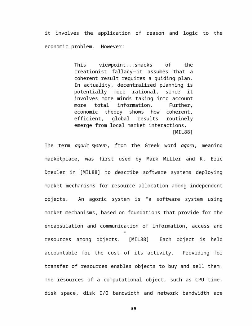
16 LocalCuts: The LocalCuts approximation algorithm, described in Section

1.1.2.2.2, which is designed to maximize pipelined parallelism.

The subplans into which the query broker divides the original plan are non-overlapping.

Dividing a plan into many small subplans increases the potential for parallel and

pipelined execution of the plan at the expense of additional communication. A query

submitted by a user demanding high performance who is willing to pay a high price

should be divided according to this strategy. Dividing a query into a few large subplans

decreases potential parallelism and pipelining while also decreasing communication

overhead. A query submitted by a user who is willing to have the query run more slowly

in return for paying a lower price should use this strategy. After dividing the plan into

subplans, the query broker determines the set of potential processing sites from which it

will solicit bids for each subplan. Site selection is performed by executing a program

written in the scripting language Tcl [OUS90]. Because the Tcl script is not compiled

into the Mariposa executable, it can be different at each site.

In Figure 16, the broker has divided the query plan into three subplans: Subplan number

1 is the scan over the EMP table; Subplan 2 is the scan over DEPT; Subplan 3 contains

the join, the sort and the aggregate. In Figure 16, the broker is soliciting bids from all

three sites for Subplan 3. The bid at each site, like site selection, is formulated by

executing a program written in Tcl. This gives each site the ability to formulate a bid in

any way it sees fit.

61

Berkeley

Fort Wayne

Fairlee

SELECT AVERAGE(EMP.SALARY), DEPT.NAMEFROM EMP, DEPTWHERE EMP.DEPTNO = DEPT.NOSORT BY DEPT.NAMEGROUP BY DEPT.NAME;

Frontend Application

Mariposa Middleware

Parser

Optimizer

Fragmenter

SQL Query

Query Plan

Home Site

Query Broker

Fragmented Query Plan

Bidder

EMP DEPTName Salary DeptNoJeff 100K 1Adam 90K 1Drew 80K 2Dave 70K 3

Name NoEngineering 1Support 2Accounting 3

EMP.Salary EMP.De ptNo100K 190K 180K 270K 3

DEPT.NameEngineeringSupportAccountingEngineering

EMP.Salary

100K90K80K

DEPT.Name

EngineeringSupportEngineering

70K Accounting

AVERAGE(Salary)95K80K

DEPT.NameEngineeringSupport

70K Accounting

Bid Curve

$

TIME

Bidder

Bidder

EMPName Salary DeptNoJeff 100K 1Adam 90K 1Drew 80K 2Dave 70K 3

Subplan #1

DEPTName NoEngineering 1Support 2Accounting 3

Subplan #2

EMP.Salary EMP.De ptNo100K 190K 180K 270K 3

DEPT.NameEngineeringSupportAccountingEngineering

EMP.Salary

100K90K80K

DEPT.Name

EngineeringSupportEngineering

70K Accounting

AVERAGE(Salary)95K80K

DEPT.NameEngineeringSupport

70K Accounting

Subplan #3

Figure 16: Long Protocol

Query brokering using the long protocol has several advantages over a traditional

distributed database management system. By creating a query plan without assigning

processing sites and then asking sites to bid, Mariposa can consider a much larger

number of sites than a traditional distributed optimizer. It has the added benefit of

allowing processing sites to consider not only the traditional cost parameters, but also

current load average, disk and memory availability, specific hardware configurations and

underlying DBMS software, administrative constraints, real-dollar costs, etc. The long

protocol also allows the system as a whole to adapt dynamically to changing resource

utilization. The processing sites may adjust their bids according to the current demand

for resources and the feedback received in the form of bids won and lost.

62

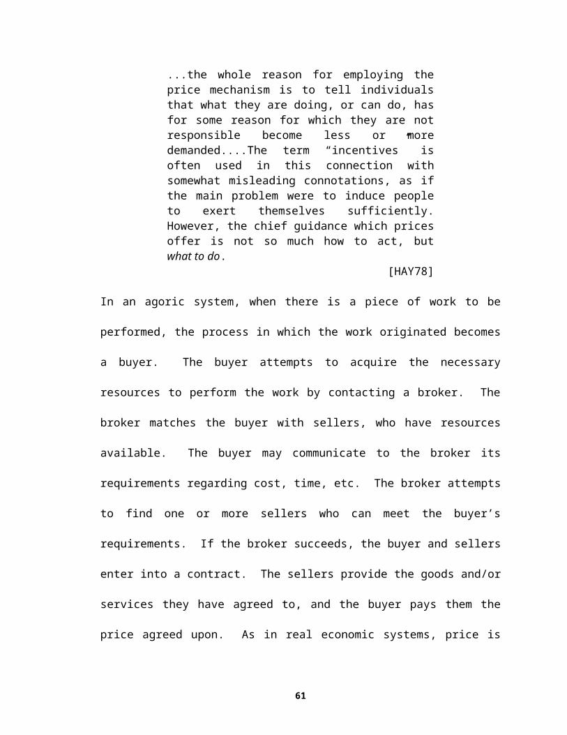
2.1.1.3.1Long Protocol vs. Short ProtocolIn order to predict when the overhead for the long protocol will become too burdensome,

it would be necessary to compare the expected execution times of a query processed

using the long protocol and using the short protocol:

timelong = brokeringlong + executionlong

timeshort = executionshort

The short protocol would be more desirable if

timeshort £ timelong

which is equivalent to

executionshort £ brokeringlong + executionlong

and

executionshort - executionlong £ brokeringlong

Machine speeds in a distributed system may vary because of differences in underlying

architectures, underlying single-site DBMS software and different loads. Only the long

protocol can guarantee that these differences will be taken into account during site

selection. In addition to performance differences, the long protocol can guarantee that

administrative constraints and user cost and performance constraints are met. The query

broker can schedule plan nodes that do not have data dependencies on any machine.

These “floating operators” can represent substantial amounts of work, as is the case with

decision-support queries, or no work at all. To determine when the long protocol is

likely to result in better performance, the relative machine speed can be factored into the

above expression for execution time. Let MAX% be the maximum difference of the

current machine speed between any two machines in a Mariposa system. Let timefloating be

the time to execute the floating operators of a query in isolation. Assume that operators

63

with data dependencies will be scheduled on the same machine by the long or short

protocol. Let timefixed be the execution time for these operators. Then the largest value of

executionshort is

timefloating * (1+MAX%) + timefixed

and the smallest possible value of timelong is

brokeringlong + timefloating + timefixed

Using the above inequality gives an expression that can be used to indicate which

protocol is likely to be more attractive:

(timefloating * (1+MAX%)) - timefloating <= timebrokering

timefloating * MAX% <= timebrokering

Therefore, if the inequality is true, then the short protocol is likely to be more attractive.

Otherwise, the long protocol should be used. This inequality can be used as a “rule of

thumb,” even though estimates of query processing time for a given query are seldom

completely accurate and the value of MAX% cannot be discovered without contacting the

various processing sites. For example, if timefloating were 1% of brokeringlong, the machine

speed difference among the servers would have to be greater than 10,000% for the long

protocol to be attractive. This is the case for queries that are typical of transaction

processing environments. If, on the other hand, timefloating were 100 times greater than

brokeringlong, the overhead of query brokering would be negligible, while the potential

benefits may be substantial. This is the case for decision support queries. For queries

whose processing times fall between these two extremes, the choice between the short

64

protocol and the long protocol is more difficult. The research presented here is based on

decision support queries. Therefore, the choice between the long and short protocols was

not an area of focus.

2.1.1.4The BidderThe bidder is the heart of a Mariposa economy. As mentioned in Section 1.1.4, price is

the mechanism by which a seller, and therefore an economy as a whole, adapts to

changing circumstances. A bidder’s goal is to maximize its income. The mechanism a

bidder has at its disposal to achieve this goal is the ability to set prices for pieces of work

sent to it by query brokers. The bidder receives feedback in the form of won or lost bids,

causing it to adjust its prices accordingly. As mentioned in Section 2.1.1.3, the bidder

script is written in Tcl. The query plan passed in to the bidder is represented as a Tcl list.

Each bidder may formulate its bid in any way. If a bidder chooses to bid, it enters into a

contract with the broker. The contract, which is recorded at both the broker and bidder

sites, simply records the work the bidder agreed to perform and the cost and time. If the

bidder wins the bidding process, it must honor its contract by performing the work within

the time it specified in the bid. After the work is performed, the bidder is paid by the

broker. The bidder records the subplan, the bid and the bid status (won or lost) in its

ledger. The bidder can use the information in the ledger to inform future bidding

policies; lowering its prices if it has lost too many bids, or raising them if it has been

awarded enough bids.

In order to make the bidder more powerful and useful, several commands have been

added to the version of Tcl used for the bidder. A complete list of these commands is in

Appendix 1. One important extension is the Subcontract command. Subcontracting

65

allows each bidder to decide which parts of a query plan it is going to process itself and

which parts it will attempt to have processed elsewhere, essentially taking the burden of

dividing up a query plan away from the broker. It is possible that a bidder may be able to

process part but not all of a subquery it is sent by the broker. For example, in Figure 17

the query broker has sent a plan representing the entire example query to Fort Wayne for

a bid. Fort Wayne has the DEPT relation, but not the EMP relation, and so can’t process

the entire query. In this case, the bidder in Fort Wayne can contact its own query broker

and solicit sub-bids from other bidder sites for the part of the plan it cannot process itself.

In Figure 17, the bidder has subcontracted a scan of the EMP relation from Berkeley. It

adds the best sub-bid into the bid it returns to the original broker site. Another benefit of

the subcontracting mechanism is that it allows network costs to be factored into the bid

sent back from the original bidder site (Fort Wayne in the example in Figure 17). When

a bidder subcontracts, it knows that the site that will process the subcontracted work is

different than itself and so can factor in the network cost.

Pricing is the mechanism by which a Mariposa system adapts to current conditions. The

next section revisits the shortcomings of traditional D-DBMSs and presents a pricing

policy designed to address each one. These policies are validated experimentally in

Section 3.

66

Berkeley

Fort Wayne

Fairlee

Home Site

Query Broker

Bidder

Bidder

Bidder

EMP DEPTName Salary DeptNoJeff 100K 1Adam 90K 1Drew 80K 2Dave 70K 3

Name NoEngineering 1Support 2Accounting 3

EMP.Salary EMP.De ptNo100K 190K 180K 270K 3

DEPT.NameEngineeringSupportAccountingEngineering

EMP.Salary

100K90K80K

DEPT.Name

EngineeringSupportEngineering

70K Accounting

AVERAGE(Salary)95K80K

DEPT.NameEngineeringSupport

70K Accounting

Query PlanEMP

Name Salary DeptNoJeff 100K 1Adam 90K 1Drew 80K 2Dave 70K 3

Subplan

Query Broker

EMPName Salary DeptNoJeff 100K 1Adam 90K 1Drew 80K 2Dave 70K 3

Subplan

Figure 17: Subcontracting

2.2PricingRecall from Section 1 the factors affecting distributed query processing performance and

other practical concerns which traditional D-DBMSs have not been able to address. Two

of these factors–resource constraints and administrative constraints–are naturally

addressed by the decision to bid or not to bid. Therefore, constraints on disk and memory

as well as administrative constraints can be addressed in a straightforward manner. When

a finite resource, such as main memory or disk space, is exhausted, a Mariposa bidder

cannot satisfy a user’s request and therefore can decline to bid. A bidder can easily be

written to reflect administrative constraints. For example, if a database administrator

doesn’t want any queries on an OLTP server between the hours of 8:00AM and 5:00PM,

the bidder at that site simply refuses to bid during these times.

The rest of the factors mentioned in Section 1 correspond to intuitive, simple pricing

mechanisms, which should lead to the correct system behavior. Each of these pricing

67

mechanisms is described in turn in the rest of this section. These mechanisms are

validated experimentally in Section 3.

2.2.1Load ImbalanceA processor’s resources can be thought of like natural resources. When demand for a

resource is high relative to availability, the price of the resource rises. By allowing

prices to reflect resource availability, Mariposa should achieve load balancing.

To test this approach to load balancing, each Mariposa bidder can formulate a bid by first

calculating a base price. The base price corresponds to the resource requirements of the

query for which the bidder is being asked to submit a bid. The base price is calculated in

a manner similar to the cost calculation in conventional query optimizer. Each node in

the query plan is assigned a cost based on its expected disk, memory and CPU

consumption. The cost of the query plan is the sum of the costs of the nodes. In order to

make price reflect resource availability, the bidder then adjusts the base price by an

inflation factor. The inflation factor should reflect the current demand for resources at

that site.

By having each bidder adjust its price according to its current resource usage, sites that

are heavily loaded will charge more to process a query than sites that are more lightly

loaded. Because the query broker awards work to the site whose bid is farthest

underneath the bid curve, heavily-loaded sites should start to lose work to more lightly-

loaded sites, achieving load balancing.

68

2.2.2Differences in Machine Speed and Underlying DBMS Capabilities Traditional cost-based distributed DBMSs and parallel DBMSs have assumed that all

processors in the system were identical. Mariposa was designed without this assumption,

and therefore must ensure that each processor participates in a manner consistent with its

hardware configuration and its underlying single-site DBMS. Mariposa’s bidding process

allows faster machines to bid low to attract more work and raise their prices more

gradually than slower machines to reflect their greater capacity. Furthermore, if a single-

site DBMS running at a Mariposa site has an efficient join algorithm, for example, the

bidder can reflect this by charging less, reflecting its relatively low resource

consumption. A simple pricing policy which should lead to good results is to cause the

base price to reflect the capacity of the machine. Fast machines become “low-cost, bulk

providers.”

2.2.3Network NonuniformityIn addition to processor speed, distributed DBMSs have assumed that network

connectivity is uniform. It is easy to imagine situations in which this is not the case.

Referring back to the example database pictured in Figure 1 if there were a group of

processors connected by a local-area network at each of the three sites, the network

bandwidth among machines that resided at a single site would most likely be much

greater than that between two machines at different locations. As mentioned in Section

2.1.1.4, when a bidder subcontracts a piece of work to another site, it adds a network tax

to its price and time estimate to reflect the network usage. The site to which work will

be subcontracted is known at the time, therefore the network connectivity is also known.

The appropriate pricing mechanism follows naturally: a high-bandwidth network

69

represents a plentiful resource and corresponds to a low network tax, while a low-

bandwidth network corresponds to a relatively high network tax. Slower networks (and

the sites connected to them) should be used less than fast ones.

2.2.4User and Cost Constraints: All of the approaches mentioned above have a single goal: to decrease response time.

However, this is not always the correct behavior. While some users may need to have

queries processed as quickly as possible, others are content to let their queries run in

batch mode, e.g. overnight. In Mariposa’s economic model, the latter users should be

able to take advantage of less expensive resources, while users demanding low response

time are likely to use more expensive processors, or to have their queries run in parallel,

thereby consuming more computational resources. The desired system behavior is to

differentiate between these two types of users and run each user’s query appropriately.

By setting the base price of a fast machine higher than that of a slow machine, the fast

machine is essentially reserved for users who are willing to pay high prices for good

performance. Users who are willing to settle for lower performance can pay less and will

be served by a less-expensive, slower machine.

In the next section, these pricing policies are validated experimentally.

70

3Experimental ResultsThis section begins with a description of the experimental environment and goes on to

describe some basic performance characteristics of Mariposa. Then, the issue of load

balancing is addressed. Load balancing is the most complex of the factors affecting

distributed query performance and is given the most attention. The effectiveness of the

simple load balancing strategy described in Section 2.2.1 is compared to a distributed

query optimizer’s ability to minimize overall resource consumption. These two

approaches are compared in scenarios with different network latencies, database sizes

and table layouts. Then, Mariposa’s load balancing strategy is compared to a strategy

devised for parallel environments. The section on load balancing ends with a comparison

of several “inflation factors” used to raise prices as resources become more heavily

utilized.

The experimental section continues with an evaluation of a simple pricing policy for

environments that include heterogeneous machines or different underlying single-site

DBMSs. A similar technique is investigated for systems with heterogeneous network

connectivity. Finally, user quality of service is addressed with pricing policies at bidder

sites that serve the needs of different classes of users.

3.1Experimental EnvironmentThe performance studies are based on the Transaction Processing Council’s benchmark

D [TPC]. This benchmark is designed to model decision-support queries. TPC-D is

widely regarded as the standard decision-support benchmark. All commercial DBMS

vendors publish TPC-D performance numbers for comparison. There are seventeen

71

queries over nine database tables (including one optional table). Unless otherwise

indicated, the database size was 10MB (corresponding to a TPC scale factor of 0.01) in

all of the experiments. The nine database tables are listed in Table 2. Mariposa does not

support nested subqueries, so the TPC-D queries were modified to eliminate them.

When a query contained a nested subquery, the subquery was replaced by a constant.

The modified TPC-D queries are included in Appendix 2.

Several of the queries in TPC-D are multi-way joins and all of them include aggregates.

For all of the Mariposa performance experiments, the single-site optimizer produced

“left-deep” plan trees, in which the inner join relation was always a base table. The plans

were sent out to potential processing sites for bids. Unless otherwise indicated, the long

protocol, presented in Section 2, was used in each experiment. The Mariposa optimizer

was an exhaustive, single-site, cost-based optimizer, like the System R optimizer

[SEL79]. The optimizer was allowed perfect information about relation sizes, selectivity

of WHERE clauses and cardinality of join results, so imperfect estimates would not

affect the outcome of the experiments. There were no indexes over any of the base

tables, so each base table access resulted in the entire table being scanned. Defining

indexes over the base relations would have affected the experimental results only

negligibly, since each query generated substantial disk I/O due to disk-based sorting of

intermediate query results. Decreasing the amount of disk I/O from base table accesses,

while it would decrease the work performed by the machine which stored the table,

would not affect the performance of Mariposa relative to the other approaches to which it

is compared.

72

TABLESIZE

(bytes)LINEITEM 11,640,832PARTSUPP 1,744,896

NATION 8,192CUSTOMER 376,832

REGION 8,192PART 442,368

SUPPLIER 24,576TIME 262,144

ORDERS 2,736,128Table 2: TPC-D Database Tables

Unless otherwise indicated, the benchmarks were run on DECStation 3000/300’s. Each

workstation had one 150 MHz Alpha/21064 processor and at least 64MB of RAM. Each

machine had between 250MB and 1GB of available disk space. Disk page size was 8192

bytes. The machines had no user processes running except the Mariposa site manager

and the single-site backend processes.

The single-site DBMS used in all of the experiments is Postgres. Postgres is not

multithreaded, therefore each subplan passed to a processing site and executed at that site

corresponds to a separate backend process. This results in more memory utilization than

would be the case with a multithreaded single-site DBMS. Because of memory

constraints, the number of backend processes at each site was limited to eight. Running

more than eight backends at a site resulted in active processes being paged out of main

memory and would have therefore affected the experimental results.

The network protocol used in Mariposa is ONC RPC over TCP/IP. All the experiments

were run over an FDDI network with a bandwidth of 100 Mb/second. Average latency

for each remote procedure call was 49 milliseconds. This overhead includes the extra

instructions at each site involved in making the remote procedure call, as well as the

actual network transmission time. The latency was highly variable, however, with a

73

maximum latency of over 1000 milliseconds and a minimum of 16 milliseconds. The

network connecting the servers is shared and therefore subject to “bursty” usage.

Network packet size for data transfers was 8192 bytes, of which 1024 bytes was header

and 7168 bytes was data.

All intersite communication, including sending tuples from one site to another during

query processing, was performed using remote procedure calls (RPCs). Flow control

was handled by buffering at the receiving site. If the receiving site ran out of buffer

space, the sending site waited until it was notified to start sending again. The amount of

buffer space available on the receiving site was 1.8MB.

3.2Basic Performance MeasurementsThis section presents some basic performance measurements for Mariposa. Because

communication among processors is a fundamental part of any distributed system,

communication overhead is discussed first. Then, the brokering imposed by Mariposa’s

long protocol is investigated. The percentage overhead for query brokering on different

database sizes is presented, followed by the effect on brokering time of increased

numbers of users and increased numbers of bidder sites. The section concludes with the

results of an experimental evaluation of the speedup per machine and the per-site

overhead imposed by Mariposa.

3.2.1Communication OverheadTo measure the overhead incurred by Mariposa’s communication protocol, table scans of

the form

SELECT COUNT(*) FROM <TABLE>;

74

were executed. The aggregate COUNT() was included in the query to avoid the

overhead of sending all the tuples to the frontend user process. The scans were initiated

at the site where the table resided (local scan) and at a remote site (remote scan). To

perform a remote table scan, the home site had to contact the name server first, which in

turn had to look up the table’s metadata and send it back. Each scan was executed once

and then timed for twenty repetitions and the average time recorded. All of the tuples

were therefore in main memory. The results are shown in Table 3. For small tables, the

communication overhead is quite large. As the table size increases, the communication

overhead becomes negligible. The setup and teardown costs for establishing and ending

RPC connections are fixed. Therefore, for small queries, they will represent a much

greater percentage of the work performed.

Table Name Table Size(bytes)

Local Time(seconds)

Remote Time(seconds)

Percentage Increase

NATION 8,192 0.024071 0.189987 1520%REGION 8,192 0.019777 0.186042 841%

SUPPLIER 24,576 0.039348 0.186969 375%CUSTOMER 376,832 0.260067 0.502194 93%

PART 442,368 0.336899 0.568888 69%PARTSUPP 1,744,896 1.45344 1.895837 30%

ORDERS 2,736,128 2.989464 3.466904 16%LINEITEM 11,640,832 9.801382 10.02327 2%

Table 3: Execution Times of Local and Remote Table Scans

To measure the relative overhead of communication setup, teardown and transfer, timing

code was inserted into the backend process to measure the elapsed time to establish an

RPC connection to a remote server, to tear down the connection, and to transfer data to

the remote site. The results of these timing tests are shown in Table 4. The transfer

time, or latency, varies by as much as 360 percent, due to varying network load.

75

Number of Network Buffers

Sent/Received

Setup Time(seconds)

Teardown Time(seconds)

Transfer Time(seconds)

Transfer Time per Network Buffer

(seconds)

1 0.001952 0.000976 0.054656 0.0546563 0.001952 0.000976 0.538752 0.179584

37 0.001952 0.000976 4.812208 0.13006185 0.001952 0.000976 5.660752 0.030599

1589 0.001952 0.000976 49.789712 0.031334Table 4: Communication Overhead During Query Processing

3.2.2Query Brokering OverheadThe long protocol, as described in Section 2, requires three rounds of messages before

query processing starts: The broker must first solicit bids from the potential bidder sites,

receive their bids, then notify the losers and the winners. In order to measure the

overhead imposed by query brokering, a Mariposa system with three sites was created.

One site was designated the home site, where all queries originated. The database tables

were distributed among the three sites as shown in Table 5.

Server Database Table(s)Remote1 LINEITEMRemote2 ORDERS

Home Site PARTSUPP, NATION, CUSTOMER, REGION, PART, SUPPLIER, TIME, ORDERS

Table 5: Data Layout for Query Brokering Experiment

The queries were sent out in their entirety by the query broker. The bidder at each

processing site subcontracted out the table scans that it could not perform. A single table

scan, such as TPC-D query number 6, shown in Figure 18, would generate five requests

for bids, and therefore five bids: three requests sent out by the home site for the whole

query, and one subcontract request each from Remote2 and the home site to Remote1 for

the scan over LINEITEM. In a system with one copy of each table and n processing sites,

a query that accesses t base tables will generate n + (n-1)t bids.

SELECT

76

float8sum(L_EXTENDEDPRICE) AS REVENUEFROM LINEITEMWHERE L_SHIPDATE >= 8767

AND L_SHIPDATE < 9132AND L_DISCOUNT >= 0.05 AND L_DISCOUNT <= 0.07AND L_QUANTITY < 24.0;

Figure 18: TPC-D Query Number Six

To measure the overhead of communication among the three sites due to the query

brokering process, timers were inserted in the Mariposa code which started timing when

the brokering process began and stopped when the last bid was received. The number of

users was varied from one to ten. Each user submitted each TPC-D query once, in

random order. The experiment was performed three times: once with a database size of

10MB, once with a size of 1MB and once with a size of 100Kb. Table 6 shows the

communication overhead for brokering vs. the average query response time for the three

database sizes.

The brokering overhead is insignificant for a database size of 10MB, and represents an

increasingly substantial amount of overhead as the database size decreases. When the

overhead becomes too great, the short protocol can be used. This would decrease the

overhead imposed by the bidding protocol, but would introduce the possibility of poor

site selection. It should be pointed out that the absolute times for the bidding protocol

are small: For ten concurrent users, the average time for the broker to complete is

around two seconds. Clearly, for most decision-support queries, this represents

acceptable overhead.

77

Number of Concurrent Users

Percentage of Total Response Time for Brokering

Database Size = 10MB Database Size = 1MB Database Size = 100Kb1 1.10% 6% 16%2 1.61% 7% 13%3 0.95% 7% 11%4 1.05% 7% 12%5 0.85% 5% 11%6 0.79% 5% 9%7 0.80% 4% 11%8 0.73% 7% 10%9 0.51% 6% 16%

10 0.65% 6% 8%Table 6: Bidding Time as a Percentage of Average Response Time

The average bidding time per query can be expected to increase as the number of users

increases, due to increased contention for network resources and CPU time. This is the

case, as shown in . The irregularity of the numbers can be attributed to variations in

network usage, as described in Section 3.1. As the number of users increases, the

average delay due to the brokering process increases, but the increase is not significant.

The average increase in brokering time per user is .1 seconds. Recall from Section 2.1

that the Mariposa broker is contained inside the Postgres backend process, and that there

is one such process for each user. Creating a multi-user broker would be likely to result

in much lower brokering overhead per user.

78

0.00

0.20

0.40

0.60

0.80

1.00

1.20

1.40

1.60

1.80

1 2 3 4 5 6 7 8 9 10Number of Concurrent Users

Ave

rage

Bro

kerin

g Ti

me

per Q

uery

(s

econ

ds)

Figure 19: Effect of Number of Users on Elapsed Brokering Time

Another factor that might be expected to increase brokering time is the number of sites

contacted. However, the brokering process for each user is multithreaded and carries out

the process of contacting bidders and receiving bid information in parallel. Each

additional bidder site should add only nominal overhead. To measure the effect the

number of bidder sites had on the brokering time, all the database tables were moved to a

single site. The number of bids per query is the same as described above. The elapsed

brokering times were measured for two and three sites. Figure 20 shows the average

brokering time for between one and five users, for two and three sites. The average

brokering time increases by an average of .6 seconds between two sites and three sites.

This increase can be attributed to additional processing time by the broker: the broker

forks off a thread for each additional processing site and allocates data structures to keep

track of the bidding process at that site.

79

0.00

0.50

1.00

1.50

2.00

2.50

3.00

3.50

4.00

4.50

5.00

1 2 3 4 5

Number of Concurrent Users

Ave

rage

Bro

kerin

g Ti

me

(sec

onds

)

Tw o Sites

Three Sites

Figure 20: Effect of Number of Bidder Sites on Elapsed Brokering Time

3.2.3Speedup and OverheadAlthough running queries across multiple machines necessarily imposes communication

overhead and, in the case of Mariposa, brokering overhead, this effect can be mitigated

by running queries in parallel. Mariposa can utilize any machine that is part of its

“economy” - that is, any machine that is running Mariposa and has registered its

existence with the rest of the system. To test the speedup that Mariposa can obtain by

using otherwise idle machines, all the database tables were placed on a single machine.

This machine also acted as the home site. There were no other machines registered in the

Mariposa system, so all the queries ran single-site. The number of users was increased

from one to ten, and the average elapsed time was recorded. A second machine was then

added and the experiment was repeated. A third machine was added, and the experiment

was repeated again. Speedup for two and three machines is calculated by dividing the

elapsed time for one machine by the elapsed time for two and three machines,

respectively. A speedup of n for n machines represents “perfect” speedup. If s is the

80

speedup obtained with n machines, the overhead per machine can be calculated as

follows:

overhead = (n - s)/n

The query broker sent out query plans to the bidder sites in their entirety; that is, without

breaking them up. The bidders formulated their bids in the following way: Upon

receiving a request to bid, a bidder would calculate the expected number of disk I/O’s

and CPU cycles to perform all the work that it could perform locally. This single-site

cost was then multiplied by (1 + LA60), where LA60 is the 60-second system load

average. The 60-second load average is the average number of jobs in the run queue

over the past sixty seconds, and is a crude measure of system performance. Bidder sites

subcontracted out operations which they could not perform locally, namely base table

accesses of remote tables. The data layout was not changed during the course of this

experiment. Therefore, all the base table accesses were performed at the home site. The

extra machines were used only to perform sorting, joins, aggregation and other such

operations. The net effect of these brokering and bidding heuristics was to assign an

entire query plan, less its leaves (which represent base table scans) to the site that is least

busy. In this way, some work can be offloaded from the home site to the other

processing sites. The bidder script used for this experiment is in Appendix 3.

By sending out plans in their entirety, the broker is limiting the parallelism achieved

during plan execution to two kinds: pipelining parallelism and inter-query parallelism.

Pipelining parallelism is achieved between a base table access and its parent node if they

are performed at different sites. The base table access is non-blocking, therefore the

81

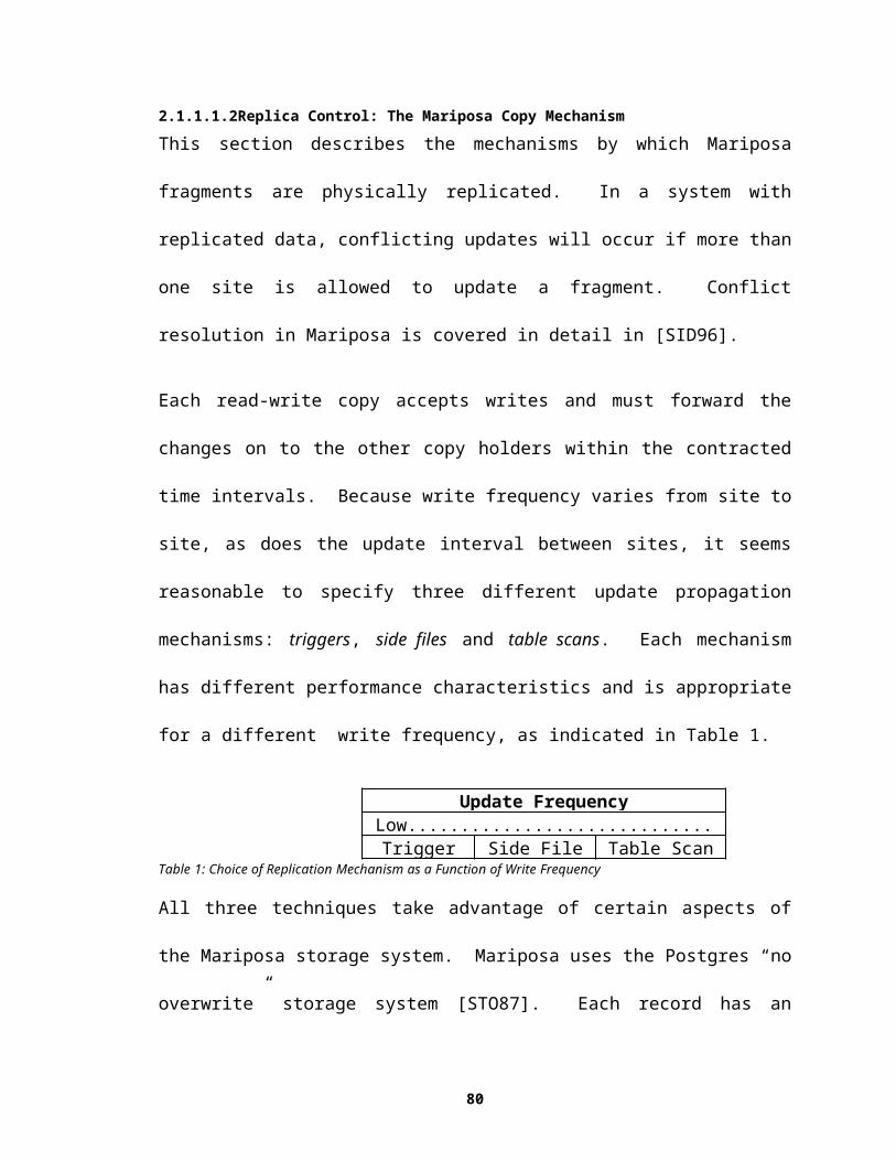
tuples can be processed by the parent node as they are received. Inter-query parallelism

is achieved by simply running two different queries on separate machines. Obviously,

this is only an option in multi-user scenarios.

It should be noted that a traditional cost-based distributed optimizer would have

produced plans which caused all the nodes in a plan tree to be executed at the home site.

In the case where all the tables are stored at one site, the lowest-cost plan is the one that

performs all the work at that site, since this will incur no communication cost.

Figure 21 shows the average response times when one, two and three machines were

made available. The Mariposa query broker was able to use the additional machines to

decrease the average response time. The effect of pipelined parallelism is apparent when

it is observed that with one user, when queries are submitted serially so there is no inter-

query parallelism, there is speedup with two machines. While the machine which stores

all the base tables is scanning a table, the second machine can be performing work in

parallel.

82

0

200

400

600

800

1000

1200

1 2 3 4 5 6 7 8 9 10

Number of Concurrent Users

Ave

rage

Res

pons

e Ti

me

Per Q

uery

(sec

onds

)

1 Site

2 Sites

3 Sites

Figure 21: Average Response Time for Mariposa Brokered Queries with 1, 2 and 3 Available Processing Sites

The average speedup for two and three machines over one machine is shown in Table 7.

Mariposa achieves nearly perfect speedup. The overhead per machine is about ten

percent.

No. of Sites Average Speedup2 1.813 2.63

Table 7: Speedup for 2 and 3 Sites with Mariposa Brokered Queries

The experiments in the section indicate that the overhead for Mariposa’s brokering

process, as well as the overhead due to communication and data exchange between sites

is not substantial. The overhead and speedup results indicate that Mariposa achieves

reasonably good speedup and imposes only limited overhead, and therefore provides a

reasonable testbed for experimentation. In the next section, the problem of load

balancing is addressed.

83

3.3Load BalancingAs described in Section 1.1.2, load balancing has been the focus of research in both

parallel and distributed database management systems. The pricing strategy by which

load balancing is achieved in Mariposa is straightforward: bidders charge more if they

are heavily-loaded and less if they are lightly-loaded. However, pricing is only one

factor that will affect the load balancing achieved. The additional communication

overhead imposed by offloading work to other sites may offset the benefit of load

balancing. The way in which query plans are divided into subplans will affect load

balancing as well.

This section begins with a comparison of Mariposa with a traditional cost-based

distributed optimizer. A cost-based distributed optimizer always produces the plan with

the lowest resource consumption. Therefore, by comparing the performance of a cost-

based optimizer to a Mariposa load balancing strategy, the overall effectiveness of this

approach can be determined. The section continues with experiments that test the effects

of network latency and query size on Mariposa’s load balancing strategy. The

effectiveness of Mariposa’s approach to load balancing is tested in a system that is

already “balanced” by virtue of its data layout. The section continues with a comparison

of Mariposa’s price-based load balancing strategy with an approximation algorithm

designed to achieve load-balancing and maximize pipelined parallelism in parallel

shared-nothing environments. Next, the effectiveness of several different pricing policies

and their ability to achieve load balancing are compared.

84

3.3.1Mariposa vs. a Static OptimizerThis experiment compared Mariposa’s load-balancing strategy to a traditional cost-based

distributed optimizer. Recall from Section 2 that Mariposa first produces a plan using a

single-site optimizer, which ignores network costs, and then schedules the query plan by

having the broker break it up and bid out the subplans. The two-phase approach is likely

to create plans that incur more communication overhead than those created by a

distributed optimizer, since a distributed optimizer includes network communication in

its cost function and can select the lowest-cost plan. However, distributed optimizers do

not include relative machine load in their cost functions. This experiment was designed

to determine whether load balancing will compensate for the fact that the distributed

plans being produced are not necessarily the lowest-cost plans.

For this experiment, the database tables were assigned to three processing sites in a

manner which balanced the load as naturally as possible without fragmenting the tables.

Each table’s size was multiplied by the number of queries in which it was accessed to

arrive at a weight. The weight was distributed among the three sites as evenly as

possible. See Table 8. The processor called Remote1 received by far the most heavily-

weighted table, and so will get a greater portion of work assigned to it.

TABLESIZE

(bytes)Number of

QueriesWEIGHT(scaled) Server

LINEITEM 11,640,832 14 1629.72 Remote1PARTSUPP 1,744,896 4 69.80 Home Site

NATION 8,192 7 0.57 Home SiteCUSTOMER 376,832 5 18.84 Home Site

REGION 8,192 2 0.16 Home SitePART 442,368 6 26.54 Home Site

SUPPLIER 24,576 9 2.21 Home SiteTIME 262,144 5 13.11 Home Site

ORDERS 2,736,128 9 246.25 Remote2Table 8: Data Layout for Load Balancing Experiment

85

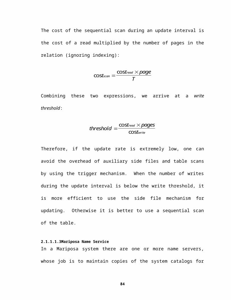
To create a cost-based distributed optimizer, the Postgres single-site optimizer’s cost

function was enhanced to include network costs. The network costs included the

additional CPU time for connection setup and teardown and the per-tuple CPU cost, as

well as the per-packet network cost of transmitting the data. The distributed optimizer

exhaustively considered all distributed plans and chose the plan which minimized its cost

function.

The Mariposa query optimization and site selection proceeded as follows: The Mariposa

optimizer produced only single-site plans, ignoring network overhead. Because the goal

of load balancing is to decrease response time, rather than decrease resource usage, the

users’ bid curves in this experiment indicated a need for quick response time and a

willingness to pay for it. A representative bid curve for this experiment is shown in .

cost

(dol

lars

)

TIME (seconds)

0

1000

0 1000

Figure 22: Bid Curve for Load Balancing Experiment

The query plans produced by the single-site optimizer were sent to bidder sites in their

entirety and each site was allowed to subcontract those nodes of the plan it could not

execute, namely scans over tables it did not own. When a site subcontracted a table scan

to another site, it added the network cost into the total bid. Sending out entire plans

minimized the bidding overhead but meant that the granularity of work assigned to each

site was very coarse.

86

The bidder for this experiment was identical to the one described in Section 3.2.3. The

bidder used LA60, the 60-second system load average (average number of jobs in the run

queue) as a crude estimate of resource consumption. The bidder at each site recursively

descended the plan tree, assigning a cost and a time estimate to each node and adding

them to arrive at a cost-based bid. The cost and time were then multiplied by (1 + LA 60).

The bidder script is in Appendix 3.

Figure 23 shows the average response time per query for queries run with the distributed

optimizer and with Mariposa’s query broker. Distributed optimization time was not

included in the response time for queries run with the distributed optimizer. In contrast to

the static distributed optimization time, the elapsed time for the brokering and bidding

process was included in the Mariposa query processing time. The The static optimizer

performed slightly better on a single query than the broker. This is to be expected, since

the static optimizer could consider network cost in assigning processing sites to the nodes

in the plans, whereas Mariposa’s single-site optimizer does not. This effect is mitigated

somewhat by the fact that the bidder adds in a network tax when a sequential scan is

subcontracted to another site. However, processing an entire query (except non-local

table scans) on the site with the lowest 60-second load average is likely to generate more

network traffic, and therefore take longer, than the plan produced by the static optimizer.

When the number of users increased, Mariposa outperformed the static optimizer. The

slope of the two lines indicates that the average response time per query for the static

optimizer will continue to degrade more quickly than that for the query broker. These

results indicate that even a simple load balancing strategy is effective in decreasing

87

response time and more than offsets the fact that the plans produced by Mariposa’s two-

phase optimization strategy are not necessarily the lowest-cost plans.

0

100

200

300

400

500

600

700

1 2 3 4 5 6 7 8 9 10

Number of Concurrent Users

Ave

rage

Res

pons

e Ti

me

Per Q

uery

(sec

onds

)

Distributed Optimizer

Brokered Queries

Figure 23: Average Response Times for Mariposa Brokered Queries vs. a Distributed Optimizer

3.3.1.1Workload Distribution in Mariposa vs. a Static OptimizerIn order to see how evenly Mariposa distributed work among the processing sites, the

amount of work performed by each site to run queries produced by the distributed

optimizer was measured and compared to the work to process brokered queries. Figure

24 shows the workload distribution among the three servers for the static optimizer, and

Figure 25 shows the same thing for Mariposa brokered queries. The X axis shows the

number of concurrent users, as in Figure 24. The Y axis shows the percentage of the

total workload performed by each server. This percentage was calculated as follows,

using the Home Site as an example:

%WORKLOADHome Site = (%CPUHome Site + %DISKHome Site + %NETHome Site) / 3

88

where:

%CPUHome Site = (CPUHome Site/(CPUHome Site + CPURemote1 + CPURemote2))

%DISKHome Site = (DISKHome Site/(DISKHome Site + DISKRemote1 + DISKRemote2))

%NETHome Site = (NETHome Site/(NETHome Site + NETRemote1 + NETRemote2))

and:

CPUmachine = total CPU time used on machine over all queries

DISKmachine = total number of disk blocks read and written on machine over all queries

NETmachine = total number of network packets sent and received by machine over all queries

Figure 24 shows that the workload was distributed among the machines consistently by

the distributed optimizer: each machine was given the same percentage of the total

workload to perform, regardless of the total amount of work. This is to be expected,

since the static optimizer produces the same plan for a query, regardless of current

conditions, and each user ran the same queries, just in a different order. The server

Remote1 has a much higher percentage of the total workload, since it contains the

largest, most heavily-used table. Remote1 therefore became a bottleneck and slowed

down query processing.

Figure 25 shows that the workload was distributed more evenly among the three

machines by the Mariposa query broker. Remote1 still performed more work than the

other two machines, but the difference among the machines is far less than for the static

optimizer. For a single user, the workload distribution is similar to that for the static

optimizer. For two users, the distribution is closer to even, and for three and more users,

the distribution has become still more even, with the difference between the work

89

performed by Remote1 and that performed by the least-burdened site, the home site,

remaining at about 15 percent.

0%

10%

20%

30%

40%

50%

60%

70%

80%

90%

100%

1 2 3 4 5 6 7 8

Number of Concurrent Users

Perc

enta

ge o

f Tot

al W

ork

per M

achi

ne

Home Site

Remote1

Remote2

Figure 24: Workload Distribution for a Distributed Optimizer

0%

10%

20%

30%

40%

50%

60%

70%

80%

90%

100%

1 2 3 4 5 6 7 8

Number of Concurrent Users

Perc

enta

ge o

f Tot

al W

ork

per M

achi

ne

Home Site

Remote1

Remote2

Figure 25: Workload Distribution for Mariposa Brokered Queries

This experiment determined that price-based load balancing can be an effective strategy

to reduce response time in a distributed DBMS. However, there are several factors that

90

may mitigate the benefits of load balancing. In the next three sections, three of those

factors are investigated.

3.3.2Effect of Network Latency on Load BalancingBecause of the overhead imposed by the brokering process, and its use of a single-site

optimizer to generate plans, Mariposa’s performance is sensitive to network delay, since

the use of a single-site optimizer cannot be guaranteed to minimize network usage. To

test Mariposa’s performance on slower networks, where network latency represents a

significant part of query processing time, the experiment described in Section 3.3.1 was

repeated with increased network latency. Network latency was increased by introducing

artificial delay for network messages and for data transfers. Each time a remote

procedure call was made or data was transmitted to a remote machine, the sending

machine delayed for a fixed period of time.

To calculate a realistic average network latency, timers were placed around the

communication modules in Mariposa. The average latency observed among the

machines connected by a local area network was 49.5 milliseconds. The TPC-D queries

were run among UC-Berkeley, UC-Santa Barbara and UC-San Diego.3 The average

latency observed among the three remote sites was 159.7 milliseconds. The artificial

network delay used for this experiment was therefore set to 110 milliseconds. The

average latency of 159.7 milliseconds was close to the median latency among the three

sites of 86 milliseconds. 110 milliseconds is greater than the latency that could be

expected from bandwidth limitations; the average observed bandwidth among the three

3 It was my original intention to run the test queries among the three remote sites. However, because of the wide variability of network latency, I could not obtain reproducible results.

91

campuses was 356 Kbps. Mariposa data streams are sent in 8K packets, resulting in an

expected delay due to bandwidth limitations of 22ms. Therefore, adding an artificial

delay of 110 milliseconds represented a reasonably realistic experimental scenario. Very

irregular, or “bursty” network utilization could be handled by adjusting the network tax

to reflect current usage.

For this experiment, the static optimizer’s cost function was changed to account for the

increase in network latency. Similarly, the network cost added in to a Mariposa bidder’s

price during subcontracting was increased. Increasing the network cost makes offloading

work from a site that is heavily used to one which is relatively idle more expensive.

Therefore, it is reasonable to expect that the effect of load balancing would be less than

when the servers were connected by a faster network.

0.00

50.00

100.00

150.00

200.00

250.00

300.00

350.00

1 2 3 4 5 6 7 8

Number of Concurrent Users

Ave

rage

Ela

psed

Tim

e Pe

r Que

ry

(sec

onds

)

Distributed Optimizer

Brokered Queries

Figure 26: Average Response Times for Mariposa Brokered Queries vs. a Static Optimizer with 110ms Network Latency

The average response times for queries run with the static optimizer and with the

Mariposa query broker are shown in Figure 26. Because of the additional network

92

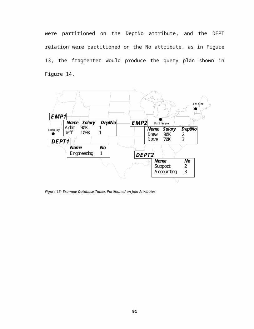
latency, and the increase in the cost of performing remote scans, the query broker was

more likely to assign a query to be processed at the site which contained most of the data

used in a query. This site (the one containing the LINEITEM table) would continue to

acquire work until its load average increased to a greater point than when the benchmark

was run over a faster network. Furthermore, there is a greater penalty if the single-site

optimizer chose a join order which necessitated excessive data movement. The

distributed optimizer could avoid such plans. In Figure 26, the query broker does not

begin to outperform the static optimizer until there are three users. Over a faster

network, as described in Section 3.3.1, the query broker outperformed the static

optimizer when there were only two users. As the network latency among the processing

sites increases, the point at which Mariposa will outperform a static optimizer also

increases.4 Figure 27 shows the workload distribution for the three servers over the

simulated long-haul network. Compared with Figure 25 the degree to which Mariposa

could effect load balancing is clearly lessened. However, the slope of the lines in Figure

26 clearly indicates that load balancing can effectively reduce response time, even when

network bandwidth is limited and communication latency is relatively high.

4 Observant readers will have noticed that the latencies in Figure 26 are smaller than those in Figure 23, even though additional network overhead was introduced. For the network delay experiments, the workstation Remote1 used in the original experiments broke down and was replaced with one that had twice the available buffer space.

93

0%

10%

20%

30%

40%

50%

60%

70%

80%

90%

100%

1 2 3 4 5 6 7 8

Number of Concurrent Users

Rel

ativ

e R

esou

rce

Usa

ge p

er M

achi

ne

Home Site

Remote1

Remote2

Figure 27: Workload Distribution for Brokered Queries Over Simulated Long-Haul Network

3.3.3Effect of Query Size on Load BalancingThe queries described in the previous sections represent substantial amounts of work.

On smaller queries, Mariposa’s brokering overhead represents a larger percentage of the

query processing time, as discussed in Section 3.2.2. Furthermore, the advantage to be

gained by more careful selection of processing sites is smaller when the amount of work

represented by a query is small. To test the value of Mariposa’s brokering strategy on

smaller queries, the experiment described in Section 3.3.1 was repeated with TPC-D

scale factors of 0.001 and 0.0001. The table sizes for these scale factors are shown

below in Table 9. All sizes are in bytes. The minimum table size is 8192, corresponding

to one disk page. All other factors remain as described in Section 3.3.1.

94

TABLE Size (bytes)Scale Factor 0.001

Size (bytes)Scale Factor 0.0001

LINEITEM 1,163,264 114,688PARTSUPP 180,224 24,576

NATION 8,192 8,192CUSTOMER 40,960 8,192

REGION 8,192 8,192PART 49,152 8,192

SUPPLIER 8,192 8,192TIME 262,144 262,144

ORDERS 278,528 32,768Table 9: Database Table Sizes for Scale Factors 0.001 and 0.0001

0.00

10.00

20.00

30.00

40.00

50.00

60.00

70.00

80.00

1 2 3 4 5 6 7 8 9 10

Number of Concurrent Users

Ave

rage

Res

pons

e Ti

me

Per Q

uery

(sec

onds

)

Static Optimizer

Brokered Queries

Figure 28: Average Response Times for Brokered Queries vs. a Distributed Optimizer for TPC-D Scale Factor 0.001

The average response time for queries run with the static optimizer and with the

Mariposa query broker for TPC-D scale factors 0.001 and 0.0001 are shown in Figure 28

and Figure 29, respectively. Because the amount of work represented by each query is

smaller than for the experiments described so far, the performance degradation for each

additional user is less. Still, Mariposa outperforms a static optimizer with relatively few

users in each case, indicating that the bidding overhead is more than compensated for by

load balancing, even for relatively small amounts of work.

95

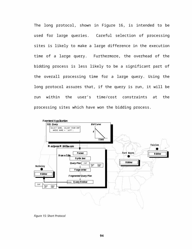
0.00

10.00

20.00

30.00

40.00

50.00

60.00

70.00

80.00

1 2 3 4 5 6 7 8 9 10

Number of Concurrent Users

Ave

rage

Res

pons

e Ti

me

Per Q

uery

(sec

onds

)

Static Optimizer

Brokered Queries

Figure 29: Average Response Times for Brokered Queries vs. a Distributed Optimizer for Scale Factor 0.0001

Interestingly, the response time degradation for the smaller data set size is more gradual

than for the larger one. The reason for this is that, since the database tables are smaller,

there is less of a natural imbalance in the load to begin with. As the absolute size of each

piece of work decreases, the opportunity to perform effective load balancing increases.

This is analogous to trying to pack three bins equally full of sand vs. trying to do the

same thing with large stones. Referring to Figure 30, the loads among the three

machines are more evenly balanced by query brokering with a scale factor 0.0001 than

for a scale factor 0.001. The relative load among the three machines remains constant for

queries run with the static optimizer.

96

Brokered Queries, Scale Factor 0.001

0%

50%

100%

1 2 3 4 5 6 7 8 9 10

Number of Concurrent Users

Rel

ativ

e R

esou

rce

Usa

ge

per M

achi

ne

Static Optimizer, Scale Factor 0.001

0%

50%

100%

1 2 3 4 5 6 7 8 9 10

Number of Concurrent Users

Rel

ativ

e R

esou

rce

Usa

ge

per M

achi

ne Home Site

Remote 1

Remote 2

Brokered Queries, Scale Factor 0.0001

0%

50%

100%

1 2 3 4 5 6 7 8 9 10

Number of Concurrent Users

Ave

rage

R

esou

rce

Usa

ge

per M

achi

ne

Static Optimizer, Scale Factor 0.0001

0%

50%

100%

1 2 3 4 5 6 7 8 9 10

Number of Concurrent Users

Ave

rage

R

esou

rce

Usa

ge

per M

achi

ne

Figure 30: Resource Utilization for Static Optimizer vs. Brokered Queries for Small Data Sets

3.3.4Effect of Data Fragmentation on Load BalancingLoad balancing can also be achieved by means other than offloading work to idle

processors, including fragmenting tables and distributing them among the processing

sites. This is a perfectly reasonable approach and is likely to obtain good results in

practice. However, fragmenting database tables and distributing the fragments does not

guarantee load balancing: one fragment can be much more heavily-used than the others.

The Mariposa approach, being adaptive, has a greater likelihood of achieving load-

balancing. Furthermore, the approach taken by Mariposa is much more general: the

tables involved in a query can be under separate administrative domains. In such a

situation, fragmentation is not an option. Another point to consider is that fragmenting

base relations does not guarantee parallel execution of subsequent operations without

repartitioning intermediate results across processors. This is the approach taken by some

parallel database management systems [GI97] and it works well to speed up a single

query but introduces substantial communication overhead and is prone to the problem of

data skew, as discussed in Section 1.1.2.2. A distributed database management system,

97

with slower intersite communication, is unlikely to benefit from this approach.

Therefore, the execution of at least some of a query plan will not be distributed among

all the available processors.

In order to test the benefits of load balancing on a system in which query processing

would be distributed evenly among the sites by virtue of data placement, the following

experiment was performed: The two tables LINEITEM and ORDER were fragmented

and distributed among the three Mariposa servers on their join attributes

(LINEITEM.L_ORDERKEY and ORDER.O_ORDERKEY). Four TPC-D queries that

would result in highly-parallelized query plans were selected. Each query was repeated

four times for a total of sixteen queries per user. The queries were run for between one

and eight users. The experiment was run first using a distributed optimizer, then repeated

using Mariposa’s long protocol.

The distributed optimizer was modified to take parallelism into account. The plans

produced by the distributed optimizer parallelized the execution of the joins as described

in Section 2.1.1.2. In each plan, all of the execution was distributed evenly among the

three servers by virtue of intra-operator parallelism with the exception of the

computation and subsequent sorting of an aggregate. The aggregate computation and

sorting were performed at the home site.

The Mariposa fragmenter produced plans identical to those produced by the distributed

optimizer, but without processing sites filled in. The query broker sent out plans in their

entirety to each bidder site. The bidder at each site attempted to maximize the parallel

execution of the plan by subcontracting joins over fragments which it didn’t own. The

98

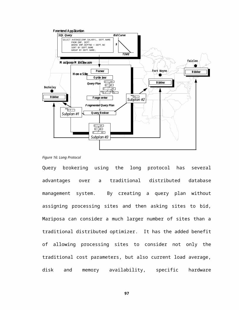
parts of a plan which a bidder chose to perform locally were priced as in Section 3.3.1:

the sum of the costs of the individual nodes was multiplied by the sixty-second load

average. The bidding and brokering times were included in the execution times for

Mariposa.

The response times for both the static and brokered experimental runs are shown in

Figure 31. As could be expected, the decrease in response time due to load balancing is

significantly less than that observed when queries were run over unfragmented data.

However, the curves in Figure 31 follow the same general pattern as those in Figure 23.

The static optimizer outperforms Mariposa when there are few users in the system. As

the number of concurrent users increases, Mariposa’s performance degrades more

gradually because of load balancing. The conclusion that can be drawn from this

experiment is that, even in situations in which the load is balanced by virtue of data

layout, the Mariposa approach will result in a slight penalty when there are few users in

the system but can improve query performance as the system becomes more heavily

loaded.

0

50

100

150

200

250

1 2 3 4 5 6 7 8

Number of Concurrent Users

Ave

rage

Ela

psed

Tim

e Pe

r Que

ry

(sec

onds

)

Distributed Optimizer

Brokered Queries

Figure 31: Comparison of Distributed Optimizer vs. Mariposa Brokered Queries on Fragmented Data

99

The experiments described so far provide evidence that Mariposa’s approach to load

balancing is beneficial in a variety of environments, including over long-haul networks

and in situations when a workload is already “balanced” by virtue of parallel data layout.

These experiments demonstrate that Mariposa’s load balancing strategy results in lower

response time than a distributed cost-based optimizer under most conditions. There are

other approaches to load balancing, as described in Section 1.1.2.2. In the next section,

Mariposa is compared with an approximation algorithm designed to maximize pipelined

parallelism and result in a balanced load. The Mariposa approach is quite simple, both in

concept and implementation. The algorithms described in Section 1.1.2.2 are less

intuitive and quite difficult to implement in practice. If the simpler Mariposa approach

performs reasonably well, then it may provide an attractive alternative to the more

complicated algorithms.

3.3.5A Comparison of Mariposa with the LocalCuts AlgorithmIn the previous sections, query plans were sent out in their entirety and then broken up by

bidders into pieces and subcontracted. The approaches taken to breaking up the queries

were simplistic: In Section 3.3.1, only the parts of a query plan which could not be

processed locally were subcontracted; in Section , the bidder took advantage of the

natural parallelism due to data fragmentation and subcontracted equal portions of a query

plan to a site which could process the subplan in its entirety. However, breaking a query

up and scheduling the subqueries optimally is NP-complete, as discussed in Section

1.1.2.2. By breaking up plans correctly, a bidder can take advantage of intra-query

parallelism. The problem of breaking up queries and scheduling them in an optimal way

100

has been studied within the context of parallel database management systems. These

approaches, if effective, could be adopted by Mariposa.

This section presents an experimental analysis of an approximation algorithm for

breaking up a query into pieces. The algorithm, called LocalCuts [CHM95], was

designed to divide queries in order to maximize pipelined parallelism in parallel shared-

nothing environments. Once the query is broken into pieces using LocalCuts, it is

scheduled using the Largest Processing Time, or LPT algorithm, as described in Section

1.1.2.2. LPT is a greedy heuristic designed to produce a processor assignment with

balanced load. This section begins with a brief description of LocalCuts. LocalCuts

makes several assumptions which had to be addressed in order to use it in a real system.

These assumptions and the changes that had to be made are discussed next, followed by a

discussion of the implementation of LocalCuts. To study the effectiveness of LocalCuts

in practice, it was implemented and compared with the more naive approaches described

previously. The experimental results obtained are described at the end of this section.

3.3.5.1The LocalCuts AlgorithmLocalCuts is presented in its entirety in [CHM95]. In LocalCuts, a query plan is

represented as a pipelined operator tree. A pipelined operator tree is composed of nodes

and edges. Each node represents an indivisible, non-blocking operation performed on

one processor. An edge represents the communication cost of sending the result of a

node to its parent. If a child node and its parent are performed on the same processor, the

edge cost is zero. Define a worthless edge as an edge whose communication cost is high

enough to offset any benefits of using parallel execution for the two end points. Define a

monotone tree as one with no worthless edges. Therefore, any two nodes in a monotone

101

tree will benefit from being scheduled on different processors. A monotone tree is

created by examining the edges of a pipelined operator tree and eliminating worthless

edges by collapsing parent and child nodes together. The cost of the resulting node is the

sum of the costs of the parent and child nodes.

LocalCuts takes a monotone tree and a parameter alpha as input and produces a set of

subtrees. The parameter alpha is used to raise the cost of an edge artificially, which will

cause some edges to become worthless. These worthless edges are eliminated by

collapsing the parent and child nodes, as described above. When there are no more

worthless edges, the nodes in the remaining tree (representing subplans from the original

query plan) are scheduled using the LPT algorithm. See Section 1.1.2.2 for a

description. The algorithm LocalCuts is shown in Figure 32. The variable cij is the cost

of communication between nodes i and j. The variable ti is the time to run operator i in

isolation, assuming no communication overhead.

Figure 32: LocalCuts Algorithm

LocalCuts has a theoretical performance bound of 3.56 when the value of alpha is set to

3.56 [CHM95]. Therefore, running LocalCuts on a query plan with alpha set to 3.56 and

scheduling the resulting subplans using the LPT algorithm should result in an execution

time that is within a factor of 3.56 of the lowest possible execution time.

102

LocalCuts:Input: Pipelined operator tree T, parameter a > 1.Output: Partition of T into fragments F1,... Fk.while there is a mother node m with a child j do

if tj > acjm then cut ejm

else collapse ejm

3.3.5.2Modifications to LocalCutsThe LocalCuts algorithm makes a few assumptions which had to be addressed before it

could be tested experimentally. First, LocalCuts assumes that all operators are non-

blocking. Second is the assumption that any operator can be scheduled on any processor;

that is, that there are no data dependencies. This is clearly not the case for base table and

temporary table accesses.

To address the issue of blocking operators, the query trees were first cut into strides (See

Section 1.1.2.2). All the operators within a stride are non-blocking and can be broken up

using LocalCuts and scheduled using LPT. To address the issue of data dependencies,

subplans produced by LocalCuts that included table accesses (and were therefore bound

to a particular site or sites) were scheduled before any other subplans in that stride. The

rest of the plan chunks in the stride were then scheduled using LPT.

3.3.5.3Implementation of LocalCutsThe LocalCuts algorithm depends on the ability to predict the single-site isolated

execution time of a node with reasonable accuracy. The execution time of an operation

run in isolation can be broken down into setup, execution, and teardown costs. For

example, the SORT operation is common and fairly straightforward. The setup costs

include calculating the number of temporary files and opening these files. The teardown

costs include deleting the temporary files. The execution cost is composed of the per-

page cost of writing/reading out a page to/from a temporary file, and the per-tuple cost of

comparing one tuple to another. To measure the setup, teardown and execution times of

various operators, “timers” were inserted around the code segments which performed

these functions for each operator. In order to estimate the execution time of two

103

operations with enough accuracy for comparison, the number of tuples processed needs

to be calculated with reasonable accuracy. The LocalCuts algorithm was allowed perfect

information about selectivity and join cardinality. The values for setup, per-tuple

execution, per-page execution and shutdown are shown in Table 10.

Operation

AGG GROUP Merge-Join Sequential Scan

(base relation)

Sequential Scan

(temp relation)

Sort UNIQUE Exchange In

Setup 0.0241 0.0260 0.0279 0.0535 0.0128 0.0155 0.0059 0.0020Per Tuple 0.0018 0.0006 0.0024 0.0012 0.0 0.0018 0.0001 0.0047Per Page 0.0 0.0 0.0055 0.0055 0.0055 0.0055 0.0 0.0

Shutdown 0.4327 0.5068 0.1973 0.0004 0.0997 0.2055 0.6071 0.0020Table 10: Timing Values for Various Node Types

In contrast to the approach taken in previous experiments, in which the division of a plan

was left up to the bidders, the home site was responsible for running LocalCuts over a

plan and then scheduling the subplans. Once a plan was broken up into strides, and the

strides were broken into subplans using LocalCuts, the subplans were scheduled using

LPT. The load average for each site was determined by contacting the sites at the

beginning of the LPT algorithm. When a subplan was scheduled on a processor, the load

average was incremented by the expected execution time for that subplan. Ideally, all the

subplans within a stride should finish at the same time. Therefore, each stride was

scheduled separately. The plan was scheduled starting at the leaf nodes and working up

towards the root, stride by stride. After all the subplans within a stride were scheduled,

the load average for each machine was re-set to its starting value and the next stride was

scheduled.

104

3.3.5.4Experimental ResultsThe data layout was the same as described in Section 3.3.1 in Table 8. The experiment

was carried out for between one and four users. As noted in Section 3.1, each Mariposa

site can only support approximately eight backend processes before it runs out of

memory. Dividing up queries into many pieces, as LocalCuts does, results in more

backend processes per site. Therefore, the number of users was limited to four.

Although the LocalCuts algorithm should perform within 3.56 of optimal when the

parameter alpha is set to 3.56, in practice the value of alpha should reflect the relative

cost of communication. The experiment was repeated five times, with alpha set to 1.1,

2.0, 3.0, 3.56 and 4.0. To test the effectiveness of LocalCuts it was compared to a much

simpler algorithm in which the query plans were broken only at blocking operators,

thereby separating them into strides, and each subplan was then scheduled as before;

placing the chunks with data dependencies on the corresponding processor and

scheduling the rest using LPT.

The elapsed times for the LocalCuts algorithm with different values of alpha are shown

in Figure 33. Also included are the previous results for brokered queries from Section

3.3.1, in which the plans were divided at the bidder sites by subcontracting remote table

accesses, and the elapsed times for the simpler algorithm, which only divided plans at

blocking operators.

105

70

80

90

100

110

120

130

140

150

1 2 3 4

Number of Concurrent Users

Ave

rage

Res

pons

e Ti

me

Per Q

uery

(s

econ

ds)

Alpha = 1.1

Alpha = 2.0

Alpha = 3.0

Alpha = 3.56

Alpha = 4.0

Breaking atBlocking OperatorsBrokered Queries

Figure 33: Comparison of LocalCuts with Mariposa Brokered Queries and Breaking Plans at Blocking Operators

The experimental results can be used to examine the effectiveness of both the LocalCuts

algorithm to maximize pipelined parallelism and also of the LPT algorithm to achieve

load balancing. The effectiveness of LocalCuts in maximizing pipelined parallelism can

be ascertained by examining the response times for a single user. In single-user mode,

the loads among the machines are likely to be more balanced to begin with, so the effect

of LPT is decreased somewhat. LocalCuts with alpha set to 3.56 outperformed the other

test runs for a single user. LocalCuts with alpha set to 3.0 performed almost as well.

Brokered queries performed better than LocalCuts for other values of alpha. The

brokered queries subcontracted sequential scans and therefore involved pipelined

parallelism between the base table access and the next operation in the plan tree, which

was usually a sort. When the value of alpha was set too low (1.1 or 2.0) or too high (4.0)

LocalCuts performed worse than subcontracting base table accesses. Setting alpha too

high eliminates worthwhile pipelined parallelism and so increases response time. The

extreme case of this is breaking plans only at blocking operators, which eliminates all

106

pipelining. When the value of alpha is low, the number of plan fragments produced by

LocalCuts is higher. When there is a relatively large number of plans to schedule, the

ability of LPT to balance the load among the processors becomes more important. The

fact that LocalCuts with alpha set to 1.1 and 2.0 performed worse than subcontracting

sequential scans only indicates that LPT was not effective in balancing the load among

the processors. This can be seen in Figure 34, which shows the relative resource

allocation among the processors for LPT and LocalCuts with alpha set to 1.1. The

resource allocation for Mariposa brokering is included for comparison.

Mariposa Brokered Queries

0%20%40%60%80%

100%

1 2 3 4

Number of Concurrent Users

Rel

ativ

e R

esou

rce

Usa

ge p

er M

achi

ne

LPT and LocalCuts with alpha = 1.1

0%20%40%60%80%

100%

1 2 3 4

Number of Concurrent Users

Rel

ativ

e R

esou

rce

Usa

ge p

er M

achi

ne

Home Site

Remote1

Remote2

Figure 34: Relative Resource Allocation for LPT Load Balancing Algorithm and Mariposa

As the number of users increases, the effect of LPT on response time is increased and the

effect of maximizing pipelining parallelism is decreased. LPT remains less effective at

balancing the load among processors than Mariposa brokering for multiple users. When

107

the number of concurrent users was greater than one, the response time for Mariposa

brokered queries was less than for LocalCuts scheduled with LPT.

When run in single-user mode, query plans produced by LocalCuts with alpha set to 3.56

led to response times that were twenty-three percent lower, on average, than query plans

produced by breaking plans at blocking operators. This performance improvement,

while not insignificant, is much less than that gained by intra-query parallelism [MD95]

[DNS91] [CG90]. The reason for this becomes clear when the query plans produced for

TPC-D queries are examined. Referring back to the example query plan shown in Figure

7, the maximum number of contiguous pipelined operators in the query plan is two. In

general, this number will be small in plans like those in the TPC-D benchmark, which

were meant to be representative of decision support queries. Such plans are composed of

several relations joined together and then one or more aggregates. Two out of the three

most common join methods (merge-sort and hash-join) involve blocking operators (sort

and hash-build, respectively). Only one common join method, nested loop join, is non-

blocking. Nested-loop joins are preferable to the other two join methods when the entire

inner relation either fits into main memory or is indexed on the join attribute. When

query plans contain few blocking operators, LocalCuts is likely to provide improved

performance by maximizing pipelined parallelism. Conversely, when the number of

contiguous pipelined operators is small, the effectiveness of LocalCuts is decreased.

The results of this experiment show that carefully dividing plans in order to maximize

pipelined parallelism can lead to some improvement in performance. The LocalCuts

algorithm could be implemented in Mariposa at the bidder sites and used to break off

108

subplans to be subcontracted. However, the performance gains that could be realized in

practice may be substantially less than those observed here. The LocalCuts algorithm,

and other approximation algorithms intended to maximize parallelism [GI97] [CHM95]

depend on accurate estimates of execution time for individual nodes in a query plan.

This is quite difficult in practice, due to the inaccuracy of selectivity estimates [ML86].

Furthermore, the LocalCuts algorithm is quite difficult to implement. Therefore, for

practical considerations, a more simplistic approach may be preferable.

In the next section, the effect of different “inflation factors” used by Mariposa bidders to

raise and lower prices is discussed.

3.3.6A Comparison of Pricing Policies for Load BalancingIn Mariposa, the price of a computational resource should reflect the availability of that

resource as accurately as possible. In this section, four different “inflation factors” are

used to raise and lower the price a bidder submits to perform a piece of work. These

factors are compared with regard to their ability to achieve load balancing.

The setup for this experiment was exactly the same as described in Section 3.3.1. The

Mariposa query broker sent out plans in their entirety, and a bidder site subcontracted out

only the parts of the plan it could not perform itself; namely, remote table scans. Four

different factors were used to raise the price and time estimate of a computation: LA60,

LA30, LA05 and ActiveBackends: the sixty-second load average, thirty-second load

average, five-second load average and number of active backend processes, respectively.

As in Section 3.3.1, each bidder recursively descended the query plan and arrived at a

base price which it then multiplied by one of the four “inflation factors.” The number of

109

users was varied between one and eight. The average response time per query, as well as

the relative resource consumption on each machine was measured and compared.

The average response times for each of the four inflation factors is shown in Figure 35,

and the relative resource consumption among the three servers for each of the three

inflation factors is shown in Figure 36. The best load balancing was achieved by using

the five-second load average to raise bidders’ prices. Five-second load average was a

more accurate estimate of resource consumption than thirty-second load average or sixty-

second load average. This seems intuitively reasonable, since a bidder’s price should

reflect the availability of resources at the current time, rather than over the past sixty or

thirty seconds. For this reason, it seems surprising that ActiveBackends performed so

poorly. The reason for this lies in the distinction between a process on the operating

system’s run queue, and an “active” backend. A backend is dedicated by a Mariposa site

manager when the site manager is notified that it has been awarded a piece of work.

However, the backend assigned to a subquery may sit idle for quite some time before it

actually performs any work. For example, referring back to the example query from

Section 1.1, if a separate backend process were dedicated to computing the AVERAGE()

function, it would wait until all the operations below it in the plan tree had finished

before it started performing work. therefore, the number of “active” backend processes

was not as accurate a measurement of system resource consumption as the number of

jobs on the run queue.

110

Varying Price by 5- and 60-Second Load Average

0

50

100

150

200

250

300

350

400

1 2 3 4 5 6 7 8

Number of Concurrent Users

Ave

rage

Res

pons

e Ti

me

Per Q

uery

(s

econ

ds) 60-Second Load Average

30-Second Load Average

5-Second Load Average

Active Backends

Figure 35: Performance Comparison of Inflation Factors

Sixty-Second Load Average

0%20%40%60%80%

100%

1 2 3 4 5 6 7 8

Number of Concurrent Users

Res

ourc

e U

sage

per

M

achi

ne Home Site

Remote1

Remote2

Five-Second Load Average

0%20%40%60%80%

100%

1 2 3 4 5 6 7 8

Number of Concurrent Users

Res

ourc

e U

sage

per

M

achi

ne

Number of Active Backends

0.000.100.200.300.400.500.60

1 2 3 4 5 6 7 8

Number of Concurrent Users

Res

ourc

e U

sage

per

M

achi

ne

Thirty-Second Load Average

0%20%40%60%80%

100%

1 2 3 4 5 6 7 8

Number of Concurrent Users

Res

ourc

e U

sage

per

M

achi

ne

Figure 36: Relative Resource Usage Among Inflation Factors

The results in this section indicate that Mariposa can achieve good load balancing in a

small-scale, controlled environment by using simple heuristics for plan division and

processor assignment. Load balancing can affect the execution time of a query

profoundly. However, there are other factors that can also affect processing time, as

mentioned in Section 2.2, as well as practical considerations which have not been met by

traditional database management systems. In the next three section, pricing mechanisms

111

that account for heterogeneous hardware, heterogeneous networks and user quality-of-

service are presented.

112

3.4Heterogeneous Environments and User Quality-of-ServiceThe pricing policy used by Mariposa to achieve load balancing is simple and intuitive: as

resources becomes more scarce, prices go up. In this section, price mechanisms that

address the issues of heterogeneous hardware and networks, as well as user quality-of-

service, are evaluated. These pricing strategies are also simple and intuitive. The first

section deals with heterogeneous hardware environments. The appeal of an effective

solution is clear: most organizations have a variety of processors, and each one should

be used in accordance with its abilities. The next section addresses environments in

which some network connections have lower bandwidth than others. This is a common

situation which arises when two offices are connected by a wide-area network. The

machines within each office are generally connected by a high-bandwidth local-area

network, which has much greater capacity than the network connecting the two offices.

The final section addresses the issue of user quality-of-service. Organizations may

include users with very different needs in terms of response time. One user may require

an answer within five minutes, while another one is content to wait until the next day, or

over a weekend. The first user’s query should be given enough computing resources to

satisfy his time constraints, perhaps by running it on a very fast or otherwise idle

machine, while the second user’s query can be run on a slower, less expensive, or more

heavily-utilized machine.

3.4.1Heterogeneous HardwareThis section presents experiments in which a Mariposa environment is composed of

heterogeneous machines. For this experiment, the server Remote2 was replaced with a

three-processor alpha with 242MB of memory. The data layout and corresponding

weights are the same as in Table 8 in Section 3.3. The faster server stored the ORDERS

table, which was the second-most heavily-used table. The ORDERS relation was split

into three fragments and each fragment was placed on a separate disk drive so that disk

accesses could be parallelized as well as CPU operations.

For this experiment, the faster server set its base price and time estimate to one-third the

levels of the other two machines under the assumption that it could handle approximately

three times the load. After a base price and a time estimate were calculated for a query

plan passed into a bidder, the price and time estimate were multiplied by the five-second

load average. Query plans were sent out by the broker in their entirety, and only remote

table accesses were subcontracted. The bid curves were also the same as in previous

sections, indicating that the users valued response time and price equally. Mariposa was

compared to a cost-based distributed optimizer. The number of users was increased from

one to eight. The average response time was measured and compared to the average

response time per query for the distributed optimizer.

The elapsed times for the distributed optimizer and for Mariposa are shown in Figure 37.

The previous results from the first load-balancing experiment, in which all three

processors were identical, are included for comparison. In single-user mode, the

distributed optimizer performs slightly better than Mariposa. When there is only a single

query in the system at a time, the three-processor machine will only use one of its

processors to execute a query. When the number of users increases, Mariposa’s

performance degrades much more gracefully than the distributed optimizer.

0

100

200

300

400

500

600

1 2 3 4 5 6 7 8

Number of Concurrent Users

Ave

rage

Res

pons

e Ti

me

per Q

uery

(sec

onds

)Distributed Optimizer,Homogeneous Environment

Brokered Queries,Homogeneous Environment

Distributed Optimizer,Heterogeneous Environment

Brokered Queries,Heterogeneous Environment

Figure 37: Elapsed Times for Distributed Optimizer and Mariposa for Heterogeneous Hardware Environment

It is interesting to compare the results of this experiment with the first load balancing

experiment, when all three processors were identical. Although the response times for the

distributed optimizer are lower when a faster processor is included in the system, the

slopes of the lines are identical, indicating that the distributed optimizer did not take

advantage of the faster processor. When the response times for Mariposa in a

homogeneous environment are compared with those for Mariposa when a faster machine

was made available, the performance degradation is more gradual in the latter

experiment. This indicates that Mariposa caused more work to be performed by the

faster machine.

The relative resource utilization among the three machines for the distributed optimizer

is shown in Figure 38. The fast processor, Remote2, was consistently given the same

amount of work to perform as in the first load balancing experiment (see Figure 24).

The resource utilization for Mariposa is shown in Figure 39. Mariposa consistently

assigned the most work to the fastest processor. In single-user mode, the faster machine

received all the work, except base table accesses. As the number of users increased, the

faster machine received approximately sixty percent of the work, while the other two

machines performed approximately one-third as much.

0%

10%

20%

30%

40%

50%

60%

70%

80%

90%

100%

1 2 3 4 5 6 7 8

Number of Concurrent Users

Rel

ativ

e R

esou

rce

Util

izat

ion

Home Site

Remote1

Remote2

Figure 38: Resource Utilization for Distributed Optimizer in Heterogeneous Hardware Environment

0%

10%

20%

30%

40%

50%

60%

70%

80%

90%

100%

1 2 3 4 5 6 7 8

Number of Concurrent Users

Rel

ativ

e R

esou

rce

Util

izat

ion

Home Site

Remote1

Remote2

Figure 39: Resource Utilization for Mariposa in a Heterogeneous Hardware Environment

The fact that the pricing policy which leads to the desired system behavior seems obvious

and that the problem of heterogeneous hardware is handled so easily by Mariposa attests

to the strength of the agoric model. In the next section, a problem very similar to

heterogeneous hardware – heterogeneous networks – is addressed in a similar fashion.

3.4.2Heterogeneous NetworksFor this experiment, the network bandwidth of one machine was lowered by changing the

network over which it communicated to the rest of the processors. This machine will be

referred to as Remote. The network over which Remote communicated was thick

Ethernet, which has a bandwidth of 10Mbps. The bandwidth between the two remaining

machines was left at 100Mbps. These machines will be referred to as Local1 and Local2.

This scenario could occur in a company with two offices, one of which contains two

processors connected by a LAN and the other of which contains a single processor. The

processors were otherwise identical. The data layout for this experiment is shown in

Table 11. Remote was the home site for this experiment.

TABLESIZE

(bytes)Number of

QueriesWEIGHT(scaled) Server

LINEITEM 11,640,832 14 1629.72 Local1

PARTSUPP 1,744,896 4 69.80 RemoteNATION 8,192 7 0.57 Remote

CUSTOMER 376,832 5 18.84 RemoteREGION 8,192 2 0.16 Remote

PART 442,368 6 26.54 RemoteSUPPLIER 24,576 9 2.21 Remote

TIME 262,144 5 13.11 RemoteORDERS 2,736,128 9 246.25 Local2

Table 11: Data Layout for Heterogeneous Network Experiment

First, the experiment was run with a distributed optimizer. The optimizer’s cost function

was altered so that the cost of network transmission reflected the average network

bandwidth in the entire network. In other words, if buffercostLocal is the cost factor for

network transmission over the fast local network, and buffercostRemote is the cost factor for

remote transmissions, the network cost factor used in the distributed optimizer was:

( cos ) cos Re23

buffer t buffer tLocal mote

After the experiment was performed with the distributed optimizer, it was repeated with

Mariposa query brokering. As before, the query broker sent out query plans in their

entirety and bidders subcontracted only remote table scans. The network tax among the

machines reflected the relative bandwidth of the network connections. The tax rate for

data transfers between Remote and either of the local machines was one hundred times

higher than the rate for transfers between the two remote machines. Tax rates were per

buffer of data transferred. The base price at each site was multiplied by the five-second

load average, therefore the system still performed some load balancing.

The average response time per query for the distributed optimizer and for Mariposa are

shown in Figure 40. The response times from the first load balancing experiment, in

which all the network connections were heterogeneous, are included for comparison.

Since the distributed optimizer’s cost function included an increased value for network

cost, network utilization was minimized. In single-user mode, the distributed optimizer

outperformed Mariposa in a heterogeneous network environment, as it did in a

homogeneous network environment. Mariposa outperformed the distributed optimizer

when the number of users increased, since it was still able to perform some load

balancing. Because of the increased network tax for communication with the remote site,

load balancing occurred between the two local machines.

0

100

200

300

400

500

600

700

1 2 3 4 5 6 7 8

Number of Concurrent Users

Ave

rage

Ela

psed

Tim

e pe

r Que

ry

(sec

onds

)

Distributed Optimizer,HeterogeneousEnvironment

Distributed Optimizer,HomogeneousEnvironment

Brokered Queries,HeterogeneousEnvironment

Brokered Queries,HomogeneousEnvironment

Figure 40: Average Response Times for Distributed Optimizer and Mariposa in Heterogeneous Network Environment

This is apparent in Figure 41, which shows the resource utilization for Mariposa brokered

queries during this experiment. The two local machines performed almost all of the

work, while the remote machine was used much less. As the number of users increased,

the remote machine performed a bit more of the work. The load on the two local

machines had to rise much higher to justify the cost of sending data across the slower

network to be processed on the remote machine.

The results of this experiment indicate that, by adjusting the network tax appropriately,

Mariposa can perform in a reasonable fashion in environments with heterogeneous

networks. The pricing policy is simple and straightforward¾the network tax should

reflect the availability of network resources¾as was the pricing policy for environments

of heterogeneous processors. In the next section, a similar approach is taken to user

quality-of service.

0%

10%

20%

30%

40%

50%

60%

70%

80%

90%

100%

1 2 3 4 5 6 7 8

Number of Concurrent Users

Ave

rage

Res

pons

e Ti

me

per Q

uery

(s

econ

ds) Remote (Home Site)

Local1

Local2

Figure 41: Resource Utilization for Mariposa in a Heterogeneous Network Environment

3.4.3User Quality-of-ServiceIn this section, a simple pricing mechanism is used in conjunction with the bid curve to

process queries in a manner which satisfies the demands of individual users. This

experiment replaced the processing site Remote2 with a three-processor DECStation, as

in Section 3.4.1. The data layout was identical to the layout in Section 3.4.1 also. The

base price for the fast machine was set three times higher than the other machines and its

response time estimate was set to one-third that of the other machines. For this

experiment, it was necessary to have two kinds of users: slow users and fast users. The

bid curve for each kind of user is shown in Figure 42. The fast users were willing to pay

very high prices and demanded low response times, while the slow users attempted to

minimize price. In this experiment, the number of users was set to ten. Three were fast

users and seven were slow users. In this experiment, Mariposa was not compared to a

distributed optimizer, since the goal was not to minimize response time overall, but to

afford appropriate quality of service to a heterogeneous user population.

As in previous experiments, the query broker sent out query plans in their entirety, and

bidders formulated their bids by assigning a base price and then inflating it using the

five-second load average. Bidders subcontracted out remote table accesses. The

network tax imposed during subcontracting was identical for each site.

$

TIME

$

TIMEFigure 42: Bid Curves for Heterogeneous Hardware Experiment

The response times for each kind of user were measured and are shown in Figure 43. As

could have been anticipated, the fast users enjoyed a response time approximately one-

third that of the slow users. Furthermore, the variation among the response times is quite

low¾eleven percent among the slow users, and five percent among the fast users.

0

50

100

150

200

250

300

Slow

Use

r 1

Slow

Use

r 2

Slow

Use

r 3

Slow

Use

r 4

Slow

Use

r 5

Slow

Use

r 6

Slow

Use

r 7

Fast

Use

r 1

Fast

Use

r 2

Fast

Use

r 3

Ave

rage

Res

pons

e Ti

me

per Q

uery

(sec

onds

)

Figure 43: Average Response Times for Heterogeneous User Population

4Conclusions and Future WorkQuery plans can be divided by the query broker, as described in Section 2.1.1.3, or by

subcontracting. Each approach has certain advantages and disadvantages. A broker

knows what a user’s bid curve looks like, so can attempt to parallelize accordingly. But

this comes at the cost of a more complex broker. A bidder doesn’t know what a bid

curve looks like, and therefore cannot attempt to subcontract in response to a particular

user’s needs. Furthermore, a bidder’s feedback consists solely of bids won and bids lost.

The bidder is not informed why it lost a bid. This approach to bidding and

subcontracting is in keeping with the central tenets of agoric systems: distribute the

decision-making process, and use price as the mechanism to influence system

behavior¾in this case, how a plan is to be divided. When a query broker decides how a

plan is to be broken up, it is doing so without the benefit of the information available to

the bidders. For example, as mentioned in Section 2.1.1.3, dividing a query up into

many small pieces increases the potential parallelism of the plan execution, thereby

decreasing response time at the expense of additional resource consumption. If a broker

divides a query plan into many fragments, several problems arise: first, if the broker

awards every piece of work to the lowest bidder, it is possible (even likely) that the same

bidder will be awarded the entire query plan, thereby defeating the purpose of breaking

up the plan in the first place. Furthermore, if the decision to break up a query is left to

the broker, the bidders will not receive feedback about the best way in which to

parallelize plans. By leaving the plan division up to each bidder, the broker distributes

the decision-making process. One bidder may be able to execute the entire query within

the user’s cost and time constraints, while another one may choose to subcontract, and

thereby parallelize, the query plan. Each bidder’s behavior will receive feedback in the

form of bids won or lost.

While an individual user’s query may not be processed in accordance with the user’s

requirements, the bidders’ behavior, and therefore the behavior of the system as a whole,

should adjust over time to meet the requirements of the user population. For example,

suppose a system’s users can be divided into two groups: “Ferraris” and “Hondas”. A

Ferrari wants her query run as fast as possible and is willing to pay a lot of money. A

Honda is less concerned about time but wants to minimize resource consumption. A

Ferrari’s query will be run by a Ferrari server, which is either a fast machine whose

bidder sets prices accordingly high, or a machine with a bidder that will divide the query

up, subcontract out pieces of the plan, and run it in parallel. Conversely, a Honda query

will be run in its entirety on a relatively slow, inexpensive machine. The population of

servers should reflect the needs of the user population. If the population of users is

largely Ferraris, then the Honda servers will lose business and adjust their pricing and

query execution strategy accordingly by either restricting the number of queries they will

run at one time, or by dividing queries up and parallelizing their execution. Both

strategies will lead to higher prices and lower execution times.

5References[AST76] Astrahan, M., et al. “System R: Relational Approach to Database

Management.” ACM Transactions on Database Systems, 1(2); 1976, 97-137.

[BER81] P. A. Bernstein, N. Goodman, E. Wong, C.L. Reeve, J. Rothnie “Query Processing in a System for Distributed Databases (SDD-1),” ACM Transactions on database Systems, 6(4), (December, 1981).

[BIT83] D. Bitton, et al “Benchmarking Database Systems: A Systematic Approach,” Proc. 1983 VLDB Conference, Florence, Italy, Nov. 1983.

[CO86] Cox, Brad J., Object Oriented Programming: An Evolutionary Approach (Addison-Wesley, Reading, MA, 1986).

[CC78] Computer Corporation of America, “Datacomputer Version 5 User Manual,” Cambridge, MA, July 1978.

[CG94] R. Cole and G. Graefe, “Optimization of Dynamic Query Evaluation Plans,” Proceedings of the 1994 ACM SIGMOD (May, 1994), pp. 150-160.

[CL86] M. Carey and H. Lu, “Load Balancing in a Locally Distributed DB System,” Proc. 1986 ACM-SIGMOD Conference on Management of Data, Washington, D.C., May 1986.

[CO70] Codd, E.F. “A Relational Model of Data for Large Shared Data Banks,” Communication of the ACM, Volume 13, no. 6 (June 1970), pp. 377-387.

[CHM95] C. Chekuri, W. Hasan, R. Motwani, “Scheduling Problems in Parallel Query Optimization,” Proceedings of the Fourteenth ACM Symposium on Principles of Database Systems (PODS), 1995, pp. 255-265.

[DAV95] D. Davison, et al. “Dynamic Resource Brokering for Multi-User Query Execution,” Proceedings of the 1995 ACM SIGMOD (May, 1995), pp. 281-92.

[DNS91] D.J. DeWitt, J.F. Naughton, D.A. Schneider, S. Seshadri, “Parallel Sorting on a Shared-Nothing Architecture Using Probabilistic Splitting.” Proc. of the First International Conference on Parallel and Distributed Information Systems, Miami, Florida (December 1991), pp. 280-291.

[DNS92] D.J. DeWitt, J.F. Naughton, D.A. Schneider, S. Seshadri, “Practical Skew Handling in Parallel Joins,” Proc. 18th VLDB Conf. (1992), pp. 27-40.

[EPS78] R. Epstein, M. Stonebraker, “Query Processing in a Distributed Data Base System,” Proceedings of the 1978 ACM-SIGMOD Conference on the Management of Data, Austin, TX, May 1978.

[GRA93] J. Gray, G. Graefe, “Transaction Processing: Concepts and Techniques,” Morgan Kaufmann Publishers, Inc. San Mateo, CA, ã1993.

[FER93] Ferguson, D. et al, “An Economy for Managing Replicated Data in Autonomous Decentralized Systems,” Proc. Int. Symp. on Autonomous Decentralized Sys. (ISADS 93), Kawasaki, Japan, Mar. 1993.

[GI97] Garofalakis, M and Ioannidis, Y. Parallel Query Scheduling and Optimization with Time- and Space-Shared Resources. Submitted for publication.

[GJ91] Garey, M and Johnson, D. Computers and Intractability. W.H. Freeman and Company, 1991. p. 65.

[GR83] Goldberg, Adele, and Robson, Dave, Smalltalk-80: The Language and its Implementation (Addison-Wesley, Reading MA, 1983).

[GRA69] R.L. Graham. “Bounds on Multiprocessing Timing Anomalies,” SIAM Journal of Applied Mathematics, 17(2):416-429, March 1969.

[GW89] G. Graefe and K. Ward, “Dynamic Query Evaluation Plans,” Proc. of the 1989 ACM SIGMOD International Conference on Management of Data, Portland, OR, (1989), p. 358.

[HAS95] W. Hasan, “Optimizing Response Time of Relational Queries by Exploiting Parallel Execution,” PhD thesis, Stanford University, 1995. In preparation.

[HAY37] Hayek, Friedrich A., “Economics and Knowledge”, from: Economica, New Series (1937) Vol. IV, pp33-54; reprinted in: Hayek, Friedrich A., (ed), Individualism and Economic Order (University of Chicago Press, Chicago, 1948).

[HAY60] Hayek, Friedrich A., The Constitution of Liberty (University of Chicago Press, Chicago, 1960) p. 156.

[HAY78] Hayek, Friedrich A., “Competition as a Discovery Procedure”, in: New Studies in Philosophy, Politics, Economics and the History of Ideas (University of Chicago Press, Chicago, 1978), p. 179-190.

[HLY93] K.A. Hua, Y. Lo, H.C. Young, “Considering Data Skew Factor in Multi-Way Join Query Optimization for Parallel Execution,” VLDB Journal 2(3) (1993), pp. 303-330.

[HM95] W. Hasan, R. Motwani, “Coloring Away Communication in Parallel Query Optimization,” 1995. Submitted for publication.

[HON92] W. Hong. “Parallel Query Processing Using Shared Memory Multiprocessors and Disk Arrays,” PhD thesis, University of California, Berkeley, August 1992.

[HUB88] Huberman, B. A. (ed.), The Ecology of Computation, North-Holland, 1988.

[HS93] W. Hong and M. Stonebraker, “Optimization of Parallel Query Execution Plans in XPRS,” Distributed and Parallel Databases, 1(1), January, 1993, p. 9.

[IOA92] Y. Ioannidis, et al. “Parametric Query Optimization,” Proceedings of the 18th International Conference on Very Large Databases (August, 1992)

[KUR89] Kurose, J. and Simha, R., “A Microeconomic Approach to Optimal Resource Allocation in Distributed Computer Systems,” IEEE Trans. on Computers 38, 5, May 1989.

[MAL88] Malone, T. W., Fikes, R. E., Grant, K.R. and Howard, M.T., “Enterprise: A Market-like Task Scheduler for Distributed Computing Environments,” in [HUB88] .

[MAR96] “The Mariposa User’s Guide,” http://mariposa.berkeley.edu (1996).

[MD95] M. Mehta, D.J. DeWitt, “Managing Intra-Operator Parallelism in Parallel Database Systems,” Proc. 21st VLDB Conf., (1995) pp. 382-394.

[MEN85] Mendelson, H. “Pricing Computer Services: Queueing Effects”, Comm. of the ACM 28,3,1985.

[MEN86] Mendelson, H. and Saharia, A.N., “Incomplete Information Costs and Database Design,” ACM Trans. on Database Systems, 11,2,1986.

[MIL88] Miller, M.S. and Drexler, K.W., “Markets and Computation: Agoric Open Systems,” in [HUB88].

[ML86] Mackert, L., and Lohman, G., “R* Optimizer Validation and Performance Evaluation for Local Queries,” Proc. 1986 ACM-SIGMOD Conference on Management of Data, Washington, D.C., June 1986.

[OUS90] J. Ousterhout. “Tcl: An Embeddable Command Language,” Proceedings of the Winter 1990 USENIX Conference (January, 1990), pp. 133-46.

[RM95] E. Rahm, R. Marek, “Dynamic Multi-Resource Load Balancing in Parallel Database Systems,” Proceedings of the 21st VLDB Conf (1995), pp. 395-406.

[RB80] Rothnie, J.B., et al, “Introduction to a System for Distributed Databases (SDD-1),” ACM Transaction on Database Systems, Vol. 5, No. 1, March 1980, pp. 1-17.

[SEL79] P. Selinger, et al. “Access Path Selection in a Relational Database Management System,” Proceedings of the 1979 ACM SIGMOD Conference on Management of Data (June, 1979).

[SEL80] P. Selinger, et al. “Access Path Selection in a Distributed Database System,” Proc. International Conference on Databases, Aberdeen, Scotland, July 1980.

[SID96] J. Sidell, et al. “Data Replication in Mariposa,” Proceedings of the 12th International Conference on Data Engineering, (February, 1996).

[STO76] M. Stonebraker, et al. “The Design and Implementation of INGRES,” ACM Transactions on Database Systems, 1(3): 189-222.

[STO83] M. Stonebraker, et al. “Performance Analysis of Distributed Data Base Systems,” Proc. of the Third Symposium on Reliability in Distributed Software and Database Systems,” October, 1983, p. 135.

[STO86] M. Stonebraker “The Design and Implementation of Distributed INGRES,” in The INGRES Papers, M. Stonebraker (ed.), Addison-Wesley, Reading, MA, 1986.

[STO87] M. Stonebraker “The Design of the Postgres Storage System,” Proceedings of the 13th International Conference on Very Large Data Bases, (September, 1987) Brighton, England, pp 289-300.

[STO88] M. Stonebraker, et al, “The Design of XPRS,” in Proc. of the fourteenth International Conference on Very Large Data Bases,” Los Angeles, CA, August, 1988.

[STO90] M. Stonebraker, et al, “On Rules, Procedures, Caching and Views in Data Base Systems”, Proc. 1990 ACM SIGMOD Conf. on Management of Data, (June, 1990) Atlantic City, NJ, pp. 281-290.

[STO91] Stonebraker, M. and G. Kemnitz, “The POSTGRES Next-Generation Database Management System,” in Communications of the ACM, 34(10): 78-92.

[STO96] M. Stonebraker, et al. “Mariposa: A Wide-Area Distributed Database System,” VLDB Journal 5, 1 (Jan. 1996), pp. 48-63.

[TPC] Transaction Processing Council, 777 N. First St. Suite 600, San Jose, CA 95112-6311. URL: www.tpc.org

[WAL92] Waldspurger, C. A., Hogg, T. et al, “Spawn: A Distributed Computational Ecology,” IEEE Trans. on Software Engineering 18,2,Feb. 1992.

[WDJ91] C.B. Walton, A.G. Dale, R.M. Jenevein, “A Taxonomy and Performance Model of Data Skew Effects in Parallel Joins,” Proc. 17th VLDB Conf. (1991) pp. 537-548.

[WDY91] J.L. Wolf, D.M. Dias, P.S. Yu, J. Turek, “An Effective Algorithm for Parallelizing Hash Joins in the Presence of Data Skew,” Proc. 7th IEEE Data Engineering Conf. (1991), pp. 200-209.

[WEL93] Wellman, M.P. “A Market-Oriented Programming Environment and Its Applications to Distributed Multicommodity Flow Problems,” Journal of AI Research 1, 1 Aug. 1993.

[WON76] Wong, E., and K. Youssefi, “Decomposition: A Strategy for Query Processing,” ACM Transactions on Database Systems, Vol. 1, No. 3, September 1976, pp. 223-241.

6Appendix 1: Mariposa Extensions to Tcl0Subcontract

Syntax subcontract plan

Input Value(s) plan: Plan to be subcontracted

Return Value(s) Bid(s) for plan; plan, with processing site(s) filled in

Description subcontract calls the Query Broker from the bidder script, passing in a query plan, which may be all or part of the plan the bidder received in a request for bid. The query broker in turn contacts other bidder sites and receives bids from them.

1movefragment

Syntax movefragment classOID, storeOID, toHostId

Input Value(s) classOID: class OID of class to which fragment belongs; storeOID: storage OID of fragment; toHostId: destination of fragment

Return Value(s) none (void)

Description Moves fragment identified by classOID, storeOID to the site identified by toHostId

2takefragmentSyntax takefragment classOID, storeOID, fromHostId

Input Value(s) classOID: class OID of class to which fragment belongs; storeOID: storage OID of fragment; fromHostId: storage site of fragment

Return Value(s) none (void)

Description Takes fragment identified by classOID, storeOID from the site identified by fromHostId

3fragidsSyntax fragids classOID

Input Value(s) classOID: class OID of a database class

Return Value(s) List of fragmentation information for each fragment in the class. The information is a list-of-lists of the form: {frastoreid fralogicalid fralocation}...

Description Looks up fragmentation information for the database class identified by classOID

4classesSyntax classes

Input Value(s) none

Return Value(s) List of all user-defined classes stored at the current site in the form {oid relname}...

Description Retrieves all user-defined classes stored at the current site.

5ReInitBidderSyntax ReInitBidder

Input Value(s) none

Return Value(s) none

Description Reinitializes the bidder. To be used if the bidder script has been been modified.

6ReInitDataBrokerSyntax ReInitDataBroker

Input Values(s) none

Return Value(s) none

Description Reinitializes the data broker. To be used if the data broker script has been modified.

7Appendix 2: Modified TPC-D Queries Used in Performance Experiments7Query #1

OriginalSELECT

L_RETURNFLAG, L_LINESTATUS, float8sum(L_QUANTITY) AS SUM_QTY,

float8sum(L_EXTENDEDPRICE) AS SUM_BASE_PRICE,float8sum(L_EXTENDEDPRICE * (1::float8 - L_DISCOUNT))

AS SUM_DISC_PRICE,float8sum(L_EXTENDEDPRICE*(1::float8 -

L_DISCOUNT)*(1::float8 + L_TAX)) AS SUM_CHARGE,float8ave(L_QUANTITY) AS AVG_QTY,

float8ave(L_EXTENDEDPRICE) AS AVG_PRICE,float8ave(L_DISCOUNT) AS AVG_DISC, COUNT(*) AS

COUNT_ORDERFROM LINEITEM

WHERE L_SHIPDATE <= (SELECT T_TIMEKEY - 90 FROM TIME WHERE T_ALPHA = '1998-12-01')

GROUP BY L_RETURNFLAG, L_LINESTATUSORDER BY L_RETURNFLAG, L_LINESTATUS;

ModifiedSELECT

L_RETURNFLAG, L_LINESTATUS, float8sum(L_QUANTITY) AS SUM_QTY,

float8sum(L_EXTENDEDPRICE) AS SUM_BASE_PRICE,float8sum(L_EXTENDEDPRICE) AS SUM_DISC_PRICE,float8sum(L_EXTENDEDPRICE) AS SUM_CHARGE,float8ave(L_QUANTITY) AS AVG_QTY,

float8ave(L_EXTENDEDPRICE) AS AVG_PRICE,float8ave(L_DISCOUNT) AS AVG_DISC, count(*) AS

COUNT_ORDERFROM LINEITEM

WHERE L_SHIPDATE <= 10427GROUP BY L_RETURNFLAG, L_LINESTATUSORDER BY L_RETURNFLAG, L_LINESTATUS;

8Query #2Original

SELECTS_ACCTBAL, S_NAME, N_NAME, P_PARTKEY, P_MFGR,

S_ADDRESS, S_PHONE, S_COMMENTFROM

PART, SUPPLIER, PARTSUPP, NATION, REGIONWHERE

P_PARTKEY = PS_PARTKEYAND S_SUPPKEY = PS_SUPPKEY

AND P_SIZE = 15AND P_TYPE ~ 'BRASS'AND S_NATIONKEY = N_NATIONKEYAND N_REGIONKEY = R_REGIONKEYAND R_NAME = 'EUROPE'AND PS_SUPPLYCOST =

(SELECT float8min(PS_SUPPLYCOST) FROM PART, PARTSUPP, SUPPLIER, NATION, REGION WHERE P_PARTKEY = PS_PARTKEY

AND S_SUPPKEY = PS_SUPPKEYAND S_NATIONKEY = N_NATIONKEYAND N_REGIONKEY = R_REGIONKEYAND R_NAME = 'EUROPE')

ORDER BY S_ACCTBAL DESC, N_NAME, S_NAME, P_PARTKEY;

ModifiedSELECT S_ACCTBAL, S_NAME, N_NAME, P_PARTKEY, P_MFGR, S_ADDRESS, S_PHONE, S_COMMENTFROM PART, SUPPLIER, PARTSUPP, NATION, REGIONWHERE P_PARTKEY = PS_PARTKEY AND S_SUPPKEY = PS_SUPPKEY AND P_SIZE = 15 AND P_TYPE ~ 'BRASS' AND S_NATIONKEY = N_NATIONKEY AND N_REGIONKEY = R_REGIONKEY AND R_NAME = 'EUROPE' AND PS_SUPPLYCOST = 50.74ORDER BY S_ACCTBAL, N_NAME, S_NAME, P_PARTKEY;

9Query #3Original

SELECTL_ORDERKEY, float8sum(L_EXTENDEDPRICE) AS REVENUE,

T_ALPHA, O_SHIPPRIORITYFROM CUSTOMER, ORDERS, LINEITEM, TIMEWHERE C_MKTSEGMENT = 'BUILDING'

AND C_CUSTKEY = O_CUSTKEYAND L_ORDERKEY = O_ORDERKEYAND O_ORDERDATE < TIMEKEY('1995-03-15')AND L_SHIPDATE > TIMEKEY('1995-03-15')

GROUP BY L_ORDERKEY, O_ORDERDATE, O_SHIPPRIORITYORDER BY REVENUE, T_ALPHA;

ModifiedSELECT

L_ORDERKEY, float8sum(L_EXTENDEDPRICE) AS REVENUE, T_ALPHA, O_SHIPPRIORITYFROM CUSTOMER, ORDERS, LINEITEM, TIMEWHERE C_MKTSEGMENT = 'BUILDING'

AND C_CUSTKEY = O_CUSTKEY

AND L_ORDERKEY = O_ORDERKEYAND O_ORDERDATE = T_TIMEKEYAND O_ORDERDATE < 9205AND L_SHIPDATE > 9205

GROUP BY L_ORDERKEY, T_ALPHA, O_ORDERDATE, O_SHIPPRIORITYORDER BY REVENUE, T_ALPHA;

10Query #4Original

SELECTO_ORDERPRIORITY, COUNT(*) AS ORDER_COUNT

FROM ORDERWHERE O_ORDERDATE >= DATE 'XXX'

AND O_ORDERDATE < DATE 'XXX' + 3 MONTHSAND EXISTS (SELECT * FROM LINEITEM

WHERE L_ORDERKEY = O_ORDERKEYAND L_COMMITDATE < L_RECEIPTDATE)

GROUP BY O_ORDERPRIORITYORDER BY O_ORDERPRIORITY;

ModifiedSELECT

O_ORDERPRIORITY, count(O_ORDERKEY) AS ORDER_COUNTFROM ORDERS, LINEITEMWHERE O_ORDERDATE >= 8583

AND O_ORDERDATE < 8675AND L_ORDERKEY = O_ORDERKEYAND L_COMMITDATE < L_RECEIPTDATE

GROUP BY O_ORDERPRIORITYORDER BY O_ORDERPRIORITY;

11Query #5Original

SELECTN_NAME, SUM(L_EXTENDEDPRICE) AS REVENUE

FROM CUSTOMER, ORDERS, LINEITEM, SUPPLIER, NATION, REGIONWHERE C_CUSTKEY = O_CUSTKEY

AND O_ORDERKEY = L_ORDERKEYAND L_SUPPKEY = S_SUPPKEYAND C_NATIONKEY = S_NATIONKEYAND S_NATIONKEY = N_NATIONKEYAND N_REGIONKEY = R_REGIONKEYAND R_NAME = 'XXX'AND O_ORDERDATE >= DATE 'XXX'AND O_ORDERDATE < DATE 'XXX' + 1 YEAR

GROUP BY N_NAMEORDER BY REVENUE;

ModifiedSELECT

N_NAME, float8sum(L_EXTENDEDPRICE) AS REVENUE

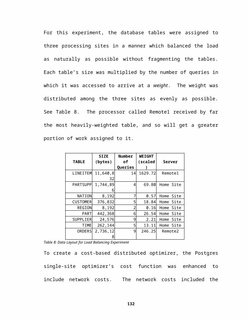
FROM CUSTOMER, ORDERS, LINEITEM, SUPPLIER, NATION, REGIONWHERE C_CUSTKEY = O_CUSTKEY

AND O_ORDERKEY = L_ORDERKEYAND L_SUPPKEY = S_SUPPKEYAND C_NATIONKEY = S_NATIONKEYAND S_NATIONKEY = N_NATIONKEYAND N_REGIONKEY = R_REGIONKEYAND R_NAME = 'ASIA'AND O_ORDERDATE >= 8767AND O_ORDERDATE < 9132

GROUP BY N_NAMEORDER BY REVENUE;

12Query #6Original

SELECTSUM(L_EXTENDEDPRICE*L_DISCOUNT) AS REVENUE

FROM LINEITEMWHERE L_SHIPDATE >= DATE 'XXX'

AND L_SHIPDATE < DATE 'XXX' + 1 YEARAND L_DISCOUNT BETWEEN YYY - 0.01 AND YYY + 0.01AND L_QUANTITY < ZZZ;

ModifiedSELECT

float8sum(L_EXTENDEDPRICE) AS REVENUEFROM LINEITEMWHERE L_SHIPDATE >= 8767

AND L_SHIPDATE < 9132AND L_DISCOUNT >= 0.05 AND L_DISCOUNT <= 0.07AND L_QUANTITY < 24.0;

13Query #7Original

SELECTSUPP_NATION, CUST_NATION, YEAR, float8sum(VOLUME) AS

REVENUEFROM (SELECT N1.N_NAME AS SUPP_NATION, N2.N_NAME AS CUST_NATION,

EXTRACT(YEAR FROM L_SHIPDATE) AS YEAR,L_EXTENDEDPRICE * (1-L_DISCOUNT) AS VOLUMEFROM SUPPLIER, LINEITEM, ORDER, CUSTOMER, NATION N1,

NATION N2WHERE S_SUPPKEY = L_SUPPKEYAND O_ORDERKEY = L_ORDERKEYAND C_CUSTKEY = O_CUSTKEYAND S_NATIONKEY = N1.N_NATIONKEYAND C_NATIONKEY = N2.N_NATIONKEYAND ((N1.N_NAME = 'XXX' AND N2.N_NAME = 'YYY') OR (N1.N_NAME = 'YYY' AND N2.N_NAME = 'XXX'))

AND L_SHIPDATE BETWEEN 1995-01-01 AND 1996-12-31) AS SHIPPINGGROUP BY SUPP_NATION, CUST_NATION, YEARORDER BY SUPP_NATION, CUST_NATION, YEAR;

ModifiedSELECT

N_NAME, N2_NAME, T_YEAR, float8sum(L_EXTENDEDPRICE) AS REVENUE

FROM SUPPLIER, LINEITEM, ORDERS, CUSTOMER, NATION, NATION2, TIMEWHERE S_SUPPKEY = L_SUPPKEY

AND O_ORDERKEY = L_ORDERKEYAND C_CUSTKEY = O_CUSTKEYAND S_NATIONKEY = N_NATIONKEYAND C_NATIONKEY = N2_NATIONKEYAND L_SHIPDATE = T_TIMEKEYAND N_NATIONKEY <> N2_NATIONKEYAND (N_NAME = 'FRANCE' OR N_NAME = 'GERMANY')AND (N2_NAME = 'FRANCE' OR N2_NAME = 'GERMANY')AND L_SHIPDATE >= 9132 AND L_SHIPDATE <= 9862

GROUP BY N_NAME, N2_NAME, T_YEARORDER BY N_NAME, N2_NAME, T_YEAR;

14Query #8Original

SELECTYEAR, SUM(CASE WHEN NATION = 'XXX'

THEN VOLUME ELSE 0 END ) / SUM(VOLUME) AS MKT_SHAREFROM

(SELECTEXTRACT(YEAR FROM O_ORDERDATE) AS YEAR,L_EXTENDEDPRICE * (1-L_DISCOUNT) AS VOLUME,

N2.N_NAME AS NATIONFROM PART, SUPPLIER, LINEITEM, ORDER, CUSTOMER, NATION

N1, NATION N2, REGIONWHERE P_PARTKEY = L_PARTKEY

AND S_SUPPKEY = L_SUPPKEYAND L_ORDERKEY = O_ORDERKEYAND O_CUSTKEY = C_CUSTKEYAND C_NATIONKEY = N1.N_NATIONKEYAND N1.N_REGIONKEY = R_REGIONKEYAND R_NAME = 'YYY'AND S_NATIONKEY = N2.N_NATIONKEYAND O_ORDERDATE BETWEEN '1995-01-01' AND

'1996-12-31'AND P_TYPE = 'ZZZ' ) ALL_NATIONS

GROUP BY YEARORDER BY YEAR;

ModifiedSELECT

T_YEAR, float8sum(L_EXTENDEDPRICE)/float8sum(L_EXTENDEDPRICE) as MKT_SHAREFROM

PART, SUPPLIER, LINEITEM, ORDERS, CUSTOMER, NATION, NATION2, REGION, TIMEWHERE

P_PARTKEY = L_PARTKEYAND S_SUPPKEY = L_SUPPKEYAND L_ORDERKEY = O_ORDERKEYAND O_CUSTKEY = C_CUSTKEYAND C_NATIONKEY = N2_NATIONKEYAND N2_REGIONKEY = R_REGIONKEYAND S_NATIONKEY = N_NATIONKEYAND O_ORDERDATE = T_TIMEKEYAND R_NAME = 'AMERICA'AND O_ORDERDATE > 9132AND O_ORDERDATE < 9862AND P_TYPE = 'ECONOMY ANODIZED STEEL'

GROUP BY T_YEARORDER BY T_YEAR;

15Query #9Original

SELECTNATION, YEAR, SUM(AMOUNT) AS SUM_PROFIT

FROM SELECTN_NAME AS NATION, YEAR(O_ORDERDATE) AS YEAR,L_EXTENDEDPRICE*(1-L_DISCOUNT) -

PS_SUPPLYCOST*L_QUANTITY AS AMOUNTFROM PART, SUPPLIER, LINEITEM, PARTSUPP, ORDER, NATIONWHERE S_SUPPKEY = L_SUPPKEY

AND PS_SUPPKEY = L_SUPPKEYAND PS_PARTKEY = L_PARTKEYAND P_PARTKEY = L_PARTKEYAND O_ORDERKEY = L_ORDERKEYAND S_NATIONKEY = N_NATIONKEYAND P_NAME LIKE 'COLOR') AS PROFIT

GROUP BY NATION, YEARORDER BY NATION, YEAR;

ModifiedSELECT

N_NAME, T_YEAR, float8sum(L_EXTENDEDPRICE)FROM PART, SUPPLIER, LINEITEM, PARTSUPP, ORDERS, NATION, TIME

WHERE S_SUPPKEY = L_SUPPKEYAND PS_SUPPKEY = L_SUPPKEYAND PS_PARTKEY = L_PARTKEYAND P_PARTKEY = L_PARTKEYAND O_ORDERKEY = L_ORDERKEYAND S_NATIONKEY = N_NATIONKEYAND O_ORDERDATE = T_TIMEKEYAND P_NAME ~ 'green'

GROUP BY N_NAME, T_YEARORDER BY N_NAME, T_YEAR;

16Query #10Original

SELECTC_CUSTKEY, C_NAME, SUM(L_EXTENDEDPRICE*(1-L_DISCOUNT))

AS REVENUE,C_ACCTBAL, N_NAME, C_ADDRESS, C_PHONE, C_COMMENT

FROM CUSTOMER, ORDER, LINEITEM, NATIONWHERE C_CUSTKEY = O_CUSTKEY

AND L_ORDERKEY = O_ORDERKEYAND O_ORDERDATE >= DATE 'XXX'AND O_ORDERDATE < DATE 'YYY' + 3 MONTHSAND L_RETURNFLAG = 'R'AND C_NATIONKEY = N_NATIONKEY

GROUP BY C_CUSTKEY, C_NAME, C_ACCTBAL, C_PHONE, N_NAME, C_ADDRESS, C_COMMENTORDER BY REVENUE;

ModifiedSELECT N_NAME, C_CUSTKEY, float8sum(L_EXTENDEDPRICE) AS REVENUEFROM CUSTOMER, ORDERS, LINEITEM, NATIONWHERE C_CUSTKEY = O_CUSTKEY AND L_ORDERKEY = O_ORDERKEY AND O_ORDERDATE >= 8675 AND O_ORDERDATE < 8767AND C_NATIONKEY = N_NATIONKEYgroup by C_CUSTKEY, N_NAMEORDER BY REVENUE;

17Query #11Original

SELECTPS_PARTKEY, SUM(PS_SUPPLYCOST*PS_AVAILQTY) AS VALUE

FROM PARTSUPP, SUPPLIER, NATIONWHERE PS_SUPPKEY = S_SUPPKEY

AND S_NATIONKEY = N_NATIONKEYAND N_NAME = 'XXX'

GROUP BY PS_PARTKEYHAVING SUM(PS_SUPPLYCOST * PS_AVAILQTY) >

(SELECTSUM(PS_SUPPLYCOST * PS_AVAILQTY) * .XXX

FROM PARTSUPP, SUPPLIER, NATION WHERE PS_SUPPKEY = S_SUPPKEY

AND S_NATIONKEY = N_NATIONKEYAND N_NAME = 'XXX')

ORDER BY VALUE;

ModifiedSELECT

PS_PARTKEY, float8sum(PS_SUPPLYCOST) AS VALUEFROM PARTSUPP, SUPPLIER, NATIONWHERE PS_SUPPKEY = S_SUPPKEY

AND S_NATIONKEY = N_NATIONKEYAND N_NAME = 'GERMANY'

GROUP BY PS_PARTKEYHAVING VALUE > 1998ORDER BY VALUE;

18Query #12Original

SELECTL_SHIPMODE, SUM(O_ORDERPRIORITY = '1-URGENT' OR

O_ORDERPRIORITY = '2-HIGH' THEN 1 ELSE 0) AS HIGH_LINE_COUNT,

SUM(O_ORDERPRIORITY <> '1-URGENT' ANDO_ORDERPRIORITY <> '2-HIGH' THEN 1 ELSE 0) AS LOW_LINE_COUNT

FROM ORDER, LINEITEMWHERE O_ORDERKEY = L_ORDERKEY

AND L_SHIPMODE IN ('MODE1', 'MODE2')AND L_COMMITDATE < L_RECEIPTDATEAND L_SHIPDATE < L_COMMITDATEAND L_RECEIPTDATE >= 'DATE'AND L_RECEIPTDATE < 'DATE' + 1YEAR

GROUP BY L_SHIPMODEORDER BY L_SHIPMODE;

ModifiedSELECT

L_SHIPMODE, count(O_ORDERPRIORITY) AS HIGH_LINE_COUNTFROM ORDERS, LINEITEMWHERE O_ORDERKEY = L_ORDERKEY

AND (O_ORDERPRIORITY = '1-URGENT' OR O_ORDERPRIORITY = '2-HIGH')AND (L_SHIPMODE = 'MAIL' OR L_SHIPMODE = 'SHIP')AND L_COMMITDATE < L_RECEIPTDATEAND L_SHIPDATE < L_COMMITDATEAND L_RECEIPTDATE >= 8767AND L_RECEIPTDATE < 9132

GROUP BY L_SHIPMODEORDER BY L_SHIPMODE;

19Query #13Original

SELECTYEAR, SUM(REVENUE) AS REVENUE

FROM (SELECTYEAR(O_ORDERDATE) AS YEAR,L_EXTENDEDPRICE * (1-L_DISCOUNT) AS REVENUE

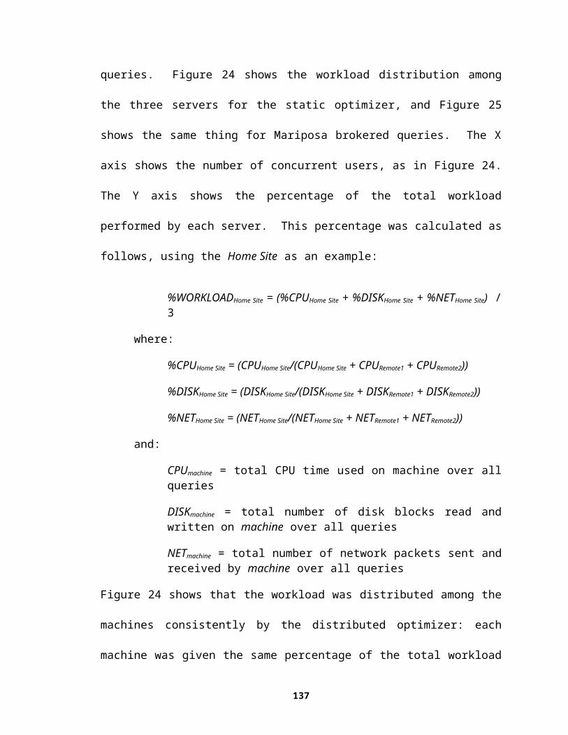
FROM LINEITEM, ORDER WHERE O_ORDERKEY = L_ORDERKEY AND O_CLERK = 'CLERK'

AND L_RETURNFLAG = 'R') AS PERFORMANCEGROUP BY YEARORDER BY YEAR;

ModifiedSELECT

T_YEAR, float8sum(L_EXTENDEDPRICE) AS REVENUEFROM LINEITEM, ORDERS, TIMEWHERE O_ORDERKEY = L_ORDERKEY

AND O_ORDERDATE = T_TIMEKEYAND O_CLERK = 'Clerk#000000088'AND L_RETURNFLAG = 'R'

GROUP BY T_YEARORDER BY T_YEAR;

20Query #14Original

SELECT100.00 * SUM(P_TYPE ~ 'PROMO%' THEN

L_EXTENDEDPRICE*(1-L_DISCOUNT) ELSE 0) / SUM(L_EXTENDEDPRICE*(1-L_DISCOUNT)) AS

PROMO_REVENUEFROM LINEITEM, PARTWHERE L_PARTKEY = P_PARTKEY

AND L_SHIPDATE >= 'DATE'AND L_SHIPDATE < 'DATE' + 1 MONTH;

ModifiedSELECT

float8sum(L_EXTENDEDPRICE) AS PROMO_REVENUEFROM LINEITEM, PARTWHERE L_PARTKEY = P_PARTKEY

AND P_TYPE ~ 'PROMO'AND L_SHIPDATE >= 9375AND L_SHIPDATE < 9405;

21Query #15Original

CREATE VIEW REVENUE (SUPPLIER_NO, TOTAL_REVENUE) ASSELECT L_SUPPKEY, SUM(L_EXTENDEDPRICE)FROM LINEITEMWHERE L_SHIPDATE >= 'DATE'

AND L_SHIPDATE < 'DATE' + 3 MONTHSGROUP BY L_SUPPKEY;

SELECT S_SUPPKEY, S_NAME, S_ADDRESS, S_PHONE, TOTAL_REVENUEFROM SUPPLIER, REVENUE

WHERE S_SUPPKEY = SUPPLIER_NOAND TOTAL_REVENUE = (SELECT MAX(TOTAL_REVENUE)

FROM REVENUE)ORDER BY S_SUPPKEY;

DROP VIEW REVENUE;

ModifiedSELECT S_SUPPKEY, S_NAME, S_ADDRESS, S_PHONE, float8sum(L_EXTENDEDPRICE) as TOTAL_REVENUE

FROM SUPPLIER, LINEITEMWHERE L_SUPPKEY = S_SUPPKEY

GROUP BY S_SUPPKEY, S_NAME, S_ADDRESS, S_PHONEORDER BY S_SUPPKEY;

22Query #16Original

SELECT DISTINCTP_BRAND, P_TYPE, P_SIZE, COUNT(PS_SUPPKEY) AS

SUPPLIER_CNTFROM PARTSUPP, PARTWHERE P_PARTKEY = PS_PARTKEY

AND P_BRAND <> 'BRAND'AND P_TYPE NOT LIKE 'TYPE'AND P_SIZE IN [SIZE1 - SIZE8]AND PS_SUPPKEY NOT IN (SELECT S_SUPPKEY FROM SUPPLIER

WHERE S_COMMENT LIKE 'BLAHBLAHBLAH')GROUP BY P_BRAND, P_TYPE, P_SIZEORDER BY SUPPLIER_CNT, P_BRAND, P_TYPE, P_SIZE;

ModifiedSELECT DISTINCT

P_BRAND, P_TYPE, P_SIZE, count(PS_SUPPKEY) AS SUPPLIER_CNTFROM PARTSUPP, PART, SUPPLIERWHERE P_PARTKEY = PS_PARTKEY

AND P_BRAND <> 'Brand#45'AND P_TYPE !~ 'MEDIUM POLISHED'AND (P_SIZE = 49 OR P_SIZE = 14 OR P_SIZE = 23 OR

P_SIZE = 45 OR P_SIZE = 19 OR P_SIZE = 3 OR P_SIZE = 36 OR

P_SIZE = 9)AND PS_SUPPKEY = S_SUPPKEYAND S_COMMENT !~ 'Better Business Bureau'

GROUP BY P_BRAND, P_TYPE, P_SIZEORDER BY SUPPLIER_CNT, P_BRAND, P_TYPE, P_SIZE;

23Query #17Original

SELECTSUM(L_EXTENDEDPRICE)/7.0 AS AVG_YEARLY

FROM LINEITEM, PARTWHERE P_PARTKEY = L_PARTKEY

AND P_BRAND = 'XXX'AND P_CONTAINER = 'YYY'AND L_QUANTITY < (SELECT 0.2 * AVG(L_QUANTITY) FROM

LINEITEM WHERE L_PARTKEY = P_PARTKEY);

ModifiedSELECT

float8sum(L_EXTENDEDPRICE)/7.0 AS AVG_YEARLYFROM LINEITEM, PARTWHERE P_PARTKEY = L_PARTKEY

AND P_BRAND = 'Brand#23'AND P_CONTAINER = 'MED BOX'AND L_QUANTITY < 6.0;

8Appendix 3: Bidder Script Used in Performance Experiments#-------------------------------------------------------------------------## bidder.tcl--# ## Copyright (c) 1994, Regents of the University of California### IDENTIFICATION# $Header: /usr/local/devel/mariposa/cvs/src/backend/sitemgr/bidder.tcl,v 1.7 1997/01/22 14:38:43 jsidell Exp $##-------------------------------------------------------------------------############################################################################# bidder.tcl## Input: plan tree, represented as a string## Output: list containing {response cost delay staleness accuracy}## response: BID if all data fragments references in the# query are local. REFUSETOBID otherwise.## cost: Based on the per-tuple and per-page charge for# each node in the query plan## delay: Based on the per-tuple and per-page delay for# each node in the query plan## staleness, accuracy: ignored## Recursively descends the plan tree, keeping track of the number of pages# and number of tuples generated, and adding up the cost and delay until# the root is reached. At this point, the total cost and total delay have# been calculated.############################################################################

set BID 1set REFUSETOBID 0set perPageNetCost 0.05

#--------------------------------------------------------------------------## CombineBids## Input: two bids, bid1 and bid2## Output: bid that results from combining bid1 and bid2:# # response: BID if both bid1 and bid2 responses are BID# REFUSETOBID otherwise## cost: bid1.cost + bid2.cost## delay: bid1.delay + bid2.delay## staleness: MAX(bid1.staleness, bid2.staleness)## accuracy: MIN(bid1.accuracy, bid2.accuracy)##--------------------------------------------------------------------------proc CombineBids {bid1 bid2} {

global BID REFUSETOBID

set response1 [lindex $bid1 0] set response2 [lindex $bid2 0] set cost1 [lindex $bid1 1] set cost2 [lindex $bid2 1] set delay1 [lindex $bid1 2] set delay2 [lindex $bid2 2] set stale1 [lindex $bid1 3] set stale2 [lindex $bid2 3] set acc1 [lindex $bid1 4] set acc2 [lindex $bid2 4]

set response [expr ($response1 && $response2) ? $BID : $REFUSETOBID] set cost [expr $cost1 + $cost2] set delay [expr $delay1 + $delay2] set stale [expr ($stale1 > $stale2) ? $stale1 : $stale2] set acc [expr ($acc1 < $acc2) ? $acc1 : $acc2]

return [list $response $cost $delay $stale $acc]

}

# Use the tclfunc fragids() to return the# fragment information for a classoid. This# will return the local fragment information, rather# than relying on what is passed in from the home site.proc GetLocalRelInfo {scanIndex fragIndex} { global nTuples global nPages global rtable global hostid

set rte [lindex $rtable $scanIndex] set classoid [lindex $rte 2] set frags [fragids $classoid] puts "***************** frags = $frags"

# Determine if one of the storage sites is this one. set local 0 foreach frag $frags {

set storageHost [lindex $frag 2]puts "***************** storageHost = $storageHost"if {[string trim $storageHost] == [string trim $hostid]} { set local 1 break}

}

set frags [lindex $rte 3] set fInfo [lindex $frags $fragIndex] set nTuples [lindex $fInfo 3] set nPages [lindex $fInfo 2]

return "$nTuples $nPages $local"}

# Use relation/fragment information passed in# from the home site via the rtable string.proc GetRelInfo {scanIndex fragIndex} { global nTuples global nPages global rtable global hostid

set rte [lindex $rtable $scanIndex] set classoid [lindex $rte 2] set frags [lindex $rte 3]

# Determine if one of the storage sites is this one. set local 0

foreach frag $frags {

puts "frag = $frag"set storageSites [lindex $frag 4]puts "storageSites = $storageSites"foreach site $storageSites { puts "site = $site" set storageHost [lindex $site 2] puts "storageHost = $storageHost" if {$storageHost == $hostid} {

set local 1 }}

}

set frags [lindex $rte 3] puts "frags = $frags" set fInfo [lindex $frags $fragIndex] puts "fragIndex = $fragIndex" puts "fInfo = $fInfo" set nTuples [lindex $fInfo 3] puts "nTuples = $nTuples" set nPages [lindex $fInfo 2]

puts "GetRelInfo: returning $nTuples $nPages $local" return "$nTuples $nPages $local"}

#--------------------------------------------------------------------------## MERGEJOIN## Input: left sub-tree, right sub-tree## Output: bid## Updates nTuples and nPages - guesses one match for each outer# tuple.#--------------------------------------------------------------------------proc MERGEJOIN {nodeNum leftTree rightTree {junk {}} } {

global BID REFUSETOBID

global nTuples global nPages global rtable global hostid

set perTupleCharge .001 set perTupleDelay .000400

set leftSubBid [CostBasedBid $leftTree] set leftTuples $nTuples set leftPages $nPages set rightSubBid [CostBasedBid $rightTree] set rightTuples $nTuples set rightPages $nPages

if {$leftTuples == 0} {set leftTuples 10000

} if {$rightTuples == 0} {

set rightTuples 10000 } if {$leftPages == 0} {

set leftPages 100 } if {$rightPages == 0} {

set rightPages 100 }

# Each outer and inner tuple is touched once. set delay [expr ($leftTuples + $rightTuples) * $perTupleDelay] set cost [expr ($leftTuples + $rightTuples) * $perTupleCharge]

# Wild guess - one match for each outer tuple set nTuples $leftTuples

set bid [CombineBids $leftSubBid $rightSubBid]

set bid [CombineBids $bid [list $BID $cost $delay 0.0 0.0]]

return $bid}#--------------------------------------------------------------------------## NESTEDLOOP## Input: left sub-tree, right sub-tree## Output: bid## Updates nTuples and nPages - guesses one match for each outer# tuple.#--------------------------------------------------------------------------proc NESTEDLOOP {nodeNum leftTree rightTree {junk {}} } {

global BID REFUSETOBID

global nTuples global nPages global rtable global hostid

set perTupleCharge .001 set perTupleDelay .000400

set leftSubBid [CostBasedBid $leftTree] set leftTuples $nTuples set leftPages $nPages set rightSubBid [CostBasedBid $rightTree] set rightTuples $nTuples set rightPages $nPages # Each inner tuple is touched once per outer tuple. set delay [expr ($leftTuples * $rightTuples) * $perTupleDelay] set cost [expr ($leftTuples * $rightTuples) * $perTupleCharge]

# Wild guess - one match for each outer tuple set nTuples $leftTuples

set bid [CombineBids $leftSubBid $rightSubBid]

set bid [CombineBids $bid [list $BID $cost $delay 0.0 0.0]]

return $bid}

#--------------------------------------------------------------------------# SEQSCAN# Input: scanIndex, fragIndex, left sub-tree## Output: bid## Updates nTuples and nPages based on information in range table.##--------------------------------------------------------------------------proc SEQSCAN {nodeNum scanIndex fragIndex {leftTree {}} } {

global BID REFUSETOBID global contract

global nTuples global nPages global rtable global hostid global perPageNetCost global subcontractOn

# no extra charge per tuple set perTupleCharge 0

# 5 cents per page set perPageCharge .05

# delay in seconds per tuple retrieved (not including disk I/O) set perTupleDelay .000600

# delay in seconds per disk page accessed set perPageDelay .002200

# Scan on a temporary relation, the result of a sort, # join, etc. Just use the values of nTuples and nPages # generated so far. if {$scanIndex == -1} {

set nTuples 10000set nPages 100set cost [expr $nTuples * $perTupleCharge + $nPages * $perPageCharge]set delay [expr $nTuples * $perTupleDelay + $nPages * $perPageDelay]

set bid [CombineBids "$BID $cost $delay 0.0 0.0" [CostBasedBid $leftTree]]

return $bid } else {

# Scan on a base relation - set nTuples and nPages# from rtable information.# Only bid if the fragment is stored at this site.

# Returns {nTuples nPages isLocal}set relInfo [GetRelInfo $scanIndex $fragIndex]

set nTuples [lindex $relInfo 0]set nPages [lindex $relInfo 1]set local [lindex $relInfo 2]

#puts "bidder.tcl: nTuples = $nTuples, nPages = $nPages"

if {$local} { set response $BID set cost [expr $nTuples * $perTupleCharge + $nPages * $perPageCharge] set delay [expr $nTuples * $perTupleDelay + $nPages * $perPageDelay]

} else { if {$subcontractOn} {

set subPlan "{SEQSCAN $nodeNum $scanIndex $fragIndex}"puts stdout "bidder.tcl: calling subcontract $subPlan $contract"flush stdoutset subBid [subcontract $subPlan $contract]set response [lindex $subBid 0]set cost [lindex $subBid 1]set delay [lindex $subBid 2]# Add in extra network cost and delayset netCost [expr $nPages * $perPageNetCost]#set netCost 0set cost [expr $cost + $netCost]puts stdout "bidder.tcl: done subcontracting $subPlan"puts stdout "subBid = $subBid"puts stdout "Adding network cost of $netCost"flush stdout

} else {set response $REFUSETOBIDset cost 0.0

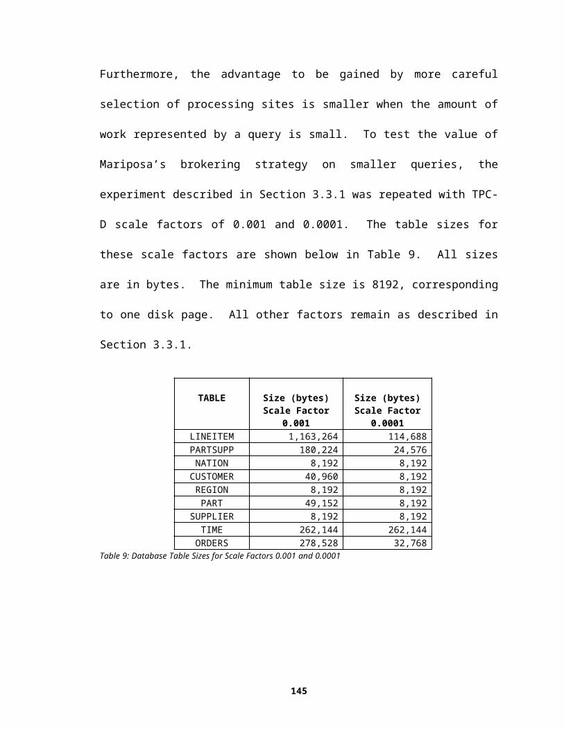
set delay 0.0 }

}

return [list $response $cost $delay 0.0 0.0]

}}

#--------------------------------------------------------------------------## SORT#--------------------------------------------------------------------------proc SORT {nodeNum baseRelId {leftTree {}} {junk2 {}} } {

global BID REFUSETOBID

global nTuples global nPages global rtable global hostid global perPageNetCost

set perTupleCharge .001 set perTupleDelay .000400 set leftSubBid [CostBasedBid $leftTree] set leftTuples $nTuples

set networkTax 0

if {$leftTuples == 0} {if {$baseRelId != -1} { # Returns {nTuples nPages isLocal} set relInfo [GetRelInfo $baseRelId 0]

puts "SORT: relInfo = $relInfo"

set nTuples [lindex $relInfo 0] set nPages [lindex $relInfo 1] set local [lindex $relInfo 2]

set leftTuples $nTuples if {!$local} {

set networkTax [expr $nPages * $perPageNetCost]puts stdout "adding in network cost of $networkTax"flush stdout

}} else { set leftTuples 10000 set nTuples 10000}

}

set cost [expr $leftTuples * $perTupleCharge + $networkTax] set delay [expr $leftTuples * $perTupleDelay] set bid "$BID $cost $delay 0.0 0.0"

set bid [CombineBids $leftSubBid $bid]

return $bid}

#--------------------------------------------------------------------------## UNIQUE#--------------------------------------------------------------------------proc UNIQUE {nodeNum {leftTree {}} {junk {}} {junk2 {}} } {

global BID REFUSETOBID

global nTuples

global nPages global rtable global hostid

set perTupleCharge .001 set perTupleDelay .000400 set leftSubBid [CostBasedBid $leftTree] set leftTuples $nTuples

if {$leftTuples == 0} {set leftTuples 10000set nTuples 10000

}

set cost [expr $leftTuples * $perTupleCharge] set delay [expr $leftTuples * $perTupleDelay] set bid "$BID $cost $delay 0.0 0.0"

set bid [CombineBids $leftSubBid $bid]

return $bid}

#--------------------------------------------------------------------------## MERGE#--------------------------------------------------------------------------proc MERGE {nodeNum subTreeList {junk {}} {junk2 {}} } {

global BID REFUSETOBID

global nTuples global nPages global rtable global hostid

set perTupleCharge .001 set perTupleDelay .000400

set bid [list $BID 0.0 0.0 0.0 0.0] set mergeTuples 0 set mergePages 0

foreach subPlan $subTreeList {set bid [CombineBids $bid [CostBasedBid $subPlan]]incr mergeTuples $nTuplesincr mergePages $nPages

} set cost [expr $mergeTuples * $perTupleCharge]

set delay [expr $mergeTuples * $perTupleDelay]

set bid [CombineBids $bid [list $BID $cost $delay 0.0 0.0]]

return $bid

}

#--------------------------------------------------------------------------## XIN#--------------------------------------------------------------------------proc XIN {nodeNum leftTree {junk {}} {junk2 {}} } {

global BID REFUSETOBID global nTuples

set perTupleCharge .001 set perTupleDelay .000400

set leftSubBid [CostBasedBid $leftTree] set leftTuples $nTuples

if {$leftTuples == 0} {

set leftTuples 10000set nTuples 10000

} set cost [expr $leftTuples * $perTupleCharge] set delay [expr $leftTuples * $perTupleDelay]

set bid "$BID $cost $delay 0.0 0.0"

set bid [CombineBids $leftSubBid $bid]

return $bid

}

#--------------------------------------------------------------------------## AGG#--------------------------------------------------------------------------proc AGG {nodeNum baseRelId leftTree {junk2 {}} } {

global BID REFUSETOBID global nTuples global perPageNetCost

set perTupleCharge .001 set perTupleDelay .000400

set leftSubBid [CostBasedBid $leftTree] set leftTuples $nTuples set networkTax 0

if {$leftTuples == 0} {if {$baseRelId != -1} { # Returns {nTuples nPages isLocal} set relInfo [GetRelInfo $baseRelId 0]

set nTuples [lindex $relInfo 0] set nPages [lindex $relInfo 1] set local [lindex $relInfo 2] set leftTuples $nTuples if {!$local} {

set networkTax [expr $nPages * $perPageNetCost]#puts stdout "adding in network cost of $networkTax"#flush stdout

}} else { set leftTuples 10000 set nTuples 10000}

}

set cost [expr $leftTuples * $perTupleCharge + $networkTax] set delay [expr $leftTuples * $perTupleDelay]

set bid "$BID $cost $delay 0.0 0.0"

set bid [CombineBids $leftSubBid $bid]

return $bid

}

#--------------------------------------------------------------------------## GROUPBY#--------------------------------------------------------------------------proc GROUPBY {nodeNum leftTree {junk {}} {junk2 {}} } {

global BID REFUSETOBID

global nTuples

set perTupleCharge .001 set perTupleDelay .000400

set leftSubBid [CostBasedBid $leftTree] set leftTuples $nTuples if {$leftTuples == 0} {

set leftTuples 10000set nTuples 10000

} set cost [expr $leftTuples * $perTupleCharge] set delay [expr $leftTuples * $perTupleDelay]

set bid "$BID $cost $delay 0.0 0.0"

set bid [CombineBids $leftSubBid $bid]

return $bid

}

#--------------------------------------------------------------------------## UNKNOWN## Don't bid on plans that contain nodes we can't identify.##--------------------------------------------------------------------------proc UNKNOWN {nodeNum leftTree rightTree {junk {}} } {

global BID REFUSETOBID

return [list $REFUSETOBID 0 0 0 0]

}

#--------------------------------------------------------------------------## CostBasedBid## Input: query plan## Output: bid## Main procedure. Looks at token representing the node type and calls# the appropriate bidding routine.##--------------------------------------------------------------------------proc CostBasedBid {plan} { global rtable global hostid global contract global nTuples global nPages

global BID REFUSETOBID

puts "CostBasedBid: plan = $plan"

if {$plan != ""} {set nodeType [lindex $plan 0]puts stdout "bidder.tcl: calling $nodeType [lindex $plan 1 ] [lindex $plan 2 ]

[lindex $plan 3 ] [lindex $plan 4]"flush stdoutset bid [$nodeType [lindex $plan 1 ] [lindex $plan 2 ] [lindex $plan 3 ] [lindex

$plan 4]]puts stdout "bidder.tcl: done with $nodeType"flush stdout

} else {

set bid [list $BID 0 0 0 0]set nTuples 0set nPages 0

}

return $bid}

#--------------------------------------------------------------------------## GetQueryBid## Input: query plan## Output: bid## Main procedure. Looks at token representing the node type and calls# the appropriate bidding routine.##--------------------------------------------------------------------------proc GetQueryBid {plan} { global rtable global hostid global contract global nTuples global nPages global homeSiteHostId global subcontractOn global BID REFUSETOBID global las global nBusyExecs

set subcontractOn true

puts "GetQueryBid: las = $las"

set bid [CostBasedBid $plan]

puts "GetQueryBid: bid = $bid"

set cost [lindex $bid 1]

puts "GetQueryBid: cost = $cost"

# las has the 5-, 30- and 60-second load averages in a list set la [lindex $las 0]

set cost [expr "$cost * (1 + $la)"]

set bid [lreplace $bid 1 1 $cost]

puts stdout "GetQueryBid returning $bid" flush stdout

return $bid}