the economics of slavery - tilburg university

TILBURG UNIVERSITY

The Economics of Slavery The Effect of the Plantation‟s Size and its Capital Utilization on the Viability of

Slavery as an Economic System

Bachelor Thesis Finance

Carina Schauland

May 2011

Student Number: S286196

Program: International Business Supervisor: M.S.D.Dwarkasing

The Economics of Slavery

2 | P a g e

Table of Contents

Table of Contents ................................................................................................................................. 2

Chapter 1: Introduction ........................................................................................................................ 3

Chapter 2: Literature Review ............................................................................................................... 5

2.1. The Economic History of Slavery in the United States ............................................................... 5

2.2. The Profitability of Southern Slavery ......................................................................................... 6

2.2.1. Evidence Against the Profitability of Slavery ...................................................................... 6

2.2.2. Evidence in Favor of the Profitability of Slavery ................................................................. 7

2.3. The Different Approaches and Measures of Profitability in Southern Slavery ............................. 9

Chapter 3: Data Analysis .................................................................................................................... 10

3.1. Hypotheses .............................................................................................................................. 11

3.2. Model ...................................................................................................................................... 11

3.3. Explanation of Variables ......................................................................................................... 12

3.3. Results .................................................................................................................................... 14

Chapter 4: Conclusion ........................................................................................................................ 20

Bibliography ...................................................................................................................................... 22

Appendix A ....................................................................................................................................... 24


3 | P a g e

Chapter 1: Introduction

The economic viability of slavery in the United States of America has been a heated

debate in economic literature, ever since Fogel and Engerman (1974) famously claimed that the

slave economy in the South was actually more productive than its free free-labor counterpart in

the North. The question thus arises whether the institution of slavery would have been able to

continue prospering, if it had not been for the civil war in 1860. The aim of this paper is to give a

deeper insight into the factors that worked in favor of the slave system in the US Antebellum

South, and which could possibly be an indication for the viability of the system. The paper

includes a data analysis of different counties in the US South in 1860, which focuses on the

profitability of slavery as labor and capital input. This analysis is based on the following main

research question;

What is the effect of the plantation’s size and its capital utilization on the viability of slavery

as an economic system?

To explain how slavery, profitability and the economic viability are interrelated I will

give some definitions of the terminology:

Slavery

“Slavery can be seen as a means of capitalizing labor” (Woodman, 1963)

“The status or condition of a person over whom any or all of the powers attaching to the

right of ownership are exercised" (Bales & Robbins, 2001)1 an

Profitability

Profit is “the difference between a firm’s sales revenue and the totality of its economic

costs, including all relevant opportunity costs” (Besanko & Braeutigam, 2008).

Woodman (1963) defines it as follows: “Profitability relates only to the success or failure

of slave production as a business and ignores the broader question of the effect of this

type of enterprise on the economy as a whole”.

1 Article 1(1) Slavery Convention of 1926


4 | P a g e

The latter quote shows that profitability becomes somewhat more difficult to define when

set in context of the viability of slavery as an economic system. It brings up the issue of making a

distinction between profitability for farms as a business versus profitability for the whole

economic system (Woodman, 1963). There are various approaches to measuring profitability of

slavery in the antebellum South, which differ substantially with the historians and economists

doing the research. More on this issue of what exactly these views on profitability are and how it

is defined will be discussed in the upcoming chapters.

Viability of an Economic System

According to Spangenberg (2005), “the viability of an economic system is defined as

being equivalent to its sustainability, and this viability is maintained if a system is able to

react adequately to changes in its system environment:”.

Since sustainability cannot be achieved if a system is not successful (presupposing the

system is analyzed as an independent unit, i.e. the sustainability of the unit depends only on its

own factors), this shows the interrelation of profitability and the economic viability of a system.

The rest of the thesis will be made up as follows. Chapter 2 includes a review of the

literature in the field of the economics of slavery. A detailed discussion of the institution of

slavery and its economic growth in the 19th century ante bellum South is presented, as well as

past research on the profitability of slavery. Chapter 3 shows a regression analysis of the main

research question; “What is the effect of the plantation‟s size and its capital utilization on the

viability of slavery as an economic system?” Chapter 4 is a conclusion about the findings from

the analysis in chapter 3 and includes recommendations for further research.


5 | P a g e

Chapter 2: Literature Review

This chapter will present a review of literature in the field of the economics of slavery. It

will start with a short introduction of the history of slavery in the Southern economy and the

Northern free-labor counterpart. Then, literature on the profitability and viability of slavery will

be discussed, concluding with a discussion of differing approaches to measure profitability.

2.1. The Economic History of Slavery in the United States

The first slaves were brought to the New World as early as the beginning of the 16th

century, and the beginning of the African slaves in America dates back to 1619. Slavery was

abolished by the 13th amendment to the constitution in 1865.

Over this time period total imports of slaves amounted to more than nine and a half

millions, of which the majority was imported during the 18th century. The high rate of slave

imports and more important, the rapid natural increase of its slave population made the U.S. the

greatest slave power of the Western world by 1825 with a distribution of 36% of all slaves in its

territories and helped finance the growth of the U.S. economy (Giles, 2006). While the Northern

part of the U.S. evolved into a free-labor manufacturing economy, the South used slaves for its

agrarian economy. The main agricultural produces were sugar, and later cotton and tobacco

which employed almost 90% of all slaves. In the 19th century cotton produced on slave

plantations in the South accounted for more than 50% of the U.S. exports. It is said that the „King

Cotton‟ made the U.S. South the world‟s leading economy at that time (Engerman & Fogel,

1974).


6 | P a g e

2.2. The Profitability of Southern Slavery

2.2.1. Evidence Against the Profitability of Slavery

For decades the main conclusion about the profitability of the Southern economy was that

it was not profitable and would have probably destroyed itself within a couple of years

(Ramsdell, 1929). While the use of coerced labor replaced the cost of labor input, and abundant

soil and favorable climate decreased the cost of capital, the lack of investment in industrialization

would have proven to be an obstacle to the sustainability of the system. What is called Southern

economic backwardness is a consequence of the destructive influence of slavery in terms of the

degrading labor market and the development of inequality (Nunn, 2007). The high competition

by slaves as labor input resulted in wages to drop below the subsistence level. This in return led

to a lack of white laborers in the market and consequently to an underdevelopment in skills levels

and prevented full utilization of potential skills (Woodman, 1963).

At the same time slave labor was economically expensive, as it required capital outlays

much larger than free labor did. While in perfectly competitive markets, workers are paid only

their marginal product, slaves had to be purchased and required maintenance costs over their

lifetime, which exceeded their marginal products; i.e. for very young and old slaves the

exploitation rate2 was negative (Vedder, 1975). Capital was tied up in the slaves, and therefore

unavailable for other investments that allowed for capital accumulation, which would have been

essential for long-term economic growth3 (Woodman, 1963). The huge capital investments were

often financed by debt. The argument that plantation work, which led to soil exhaustion, was an

indicator for the decadence of slavery, assuming that slavery was limited to the agricultural

sector, persists and is supported by the westward redistribution of the slave population and

farming from the late 18th until the late 19th century (Engerman & Fogel, 1974). Chapter 3 will

take a closer look on the impact of a plantation‟s soil quality on overall profits.

2 According to Vedder (1975) the exploitation rate can be defined in the Marxian definition as the difference between the wage rate and the value

of the average output per worker, or in the Robinsonian definition as difference between the wage rate and the value of the marginal product of slaves divided by the value of the marginal product. 3 According to the Solow model, economic growth depends on capital accumulation (Stein, 2007). Furthermore, Adam Smith that “key elements

in the growth process are the nature, accumulation, and employment of stock”. ( Ekelund & Hebert, 1997)


7 | P a g e

2.2.2. Evidence in Favor of the Profitability of Slavery

The fact that slavery in the South existed and prospered for more than two hundred years

should imply that there is some evidence in favor of the productivity and maintainability of

slavery. One of the most famous and debated works on the economics of slavery is written by

Robert W. Fogel and Stanley L. Engerman (1970). They claim that slavery was indeed a

profitable and viable system, because total factor productivity in the South was 9.2 % higher than

in the North. This conclusion is based on the high productivity of slavery as capital input, profits

regarding slave trade, and a high growing per capita income in the South. Their study on the

profitability of the South and its economy stresses the importance of the exploitation rate of slave

workers, and the market situation for exports of output. The fact that plantation owners had

property rights in slaves, allowed for extensively high exploitation rates. Force, supervision and

child labor implies that slave or coerced labor could be exploited much more than free labor and

thus, could make up for the higher capital costs. According to findings of Fenoaltea (1984) and

Acemoglu & Wolitzky (2009), coercion always motivates effort-intensive work. Even though

production sky rocked while cotton prices fell steadily in preceding era of the civil war,

Engerman and Fogel (1974) show that profits of cotton production were above normal levels. An

explanation could be that demand for cotton always succeeded supply on average, while prices

for cotton stayed above normal levels4. This was especially a predominant phenomenon between

1850 and 1860, which leads to no conclusion that unprofitability could have been a force in the

self-destruction of slavery.

Another indicator for the maintainability of slavery as an economic system is the fact that

the more productive regions of the South were the ones that specialized in agricultural

production, while the less productive regions produced slaves for trade in order to make these

regions more competitive (Conrad& Meyer, 1958). Also, the use of the cotton gin can be seen as

a technological improvement that increased its marginal productivity of slaves as capital. This

emphasizes, if even in an abstract way, the potential for flexibility of the economy to react to

4 Engerman, S. L., & Fogel, R. W. (1974). Time on the Cross: The Economics of American Negro Slavery. London: Wildwood House Limited. Page 92. Figure 27 “The deviation of cotton prices from their trend value 1802-1861”, Figure 28 “A comparison between indexes of cotton demanded and supplied, 1829-1861”


8 | P a g e

different situations, as it shows a successful adjustment of the economy to shifting labor

requirements (Engerman & Fogel, 1974), and the trend to increase productivity. This is in line

with the definition given by Spangenberg (2005) who specifies the viability of a system as “being

equivalent to its sustainability, and viability is maintained if a system is able to react adequately

on changes in its system environment”.

The rate of return that various farms of different size and in different regions accounted,

propose that the profits were sufficient enough for an investment in industrialization (Conrad&

Meyer, 1958) Thus, the argument that slavery was the sole obstacle to industrialization has to be

omitted. In fact, “the relative absence of industrial and urban development in the Southern USA

[…] was simply the result of these regions’ comparative advantages in agricultural production”

(Post, 2003).

Against the argument that slave labor was only profitable because of the high exploitation

rates, stands the following discussion: Because slavery united labor and capital, the slave was

better off than the wage slave in the North, according to George Fitzhugh (1857). He was

provided food and shelter, which were calculated as being more advantageous for the slave

population (average daily slave diet made up 111% of the free person‟s diet (Engerman & Fogel,

1974)). Regardless of the accuracy of these calculations when taking into account the labor

circumstances, these costs can be accounted as a wage paid to the slave, and thus, the labor input

was not free of costs for the plantation owners. Consequently, differences in exploitation rates

between Southern slaves and Northern free laborers are less than a horrendous amount

(Engerman & Fogel, 1974). Yet, estimates on the exploitation rate differ significantly between

researchers and can therefore not be taken into account as a reliable source to evaluate

profitability of labor input in this paper.

The Southern plantation economy is said to have been a pioneer in routinizing labor by

task division and effective supervision of the labor force, which led to efficient methods of

production (Woodman, 1963). Moreover, the Southern agriculture was indisputably the main

contributor to the United States exports, composed of cotton and tobacco, during that time span

(Engerman & Fogel, 1974). 87% of the slaves in 1850 were employed in the cotton and tobacco

sector. If treated as a separate nation, the South had been the fourth richest country in the world

during that time (Engerman & Fogel, 1974), and it is argued that Northern profits actually

depended upon Southern wealth (Kettell, 1860). If this argument is true, the Southern economy


9 | P a g e

deserves, regardless of its own profitability, some credit for the generally accepted profitability of

the Northern economy. Finally, Post (2003) found that per capita income actually grew slightly

more rapid than in the North during the last two decades preceding the Civil War.

2.3. The Different Approaches and Measures of Profitability in Southern Slavery

Following from the previous discussion, it becomes obvious that profitability can be

measured in a number of ways, because there is the complex issue of defining the area that is

investigated on profitability. Is it limited to the individual farm level, the Southern states, the

United States as a whole, or even includes other economies such as the British Empire, who

profited from the slave market?5 The question whether measures of profitability should take into

account only white farmers or the whole population will not be discussed in this paper, as it

brings up issues of morality and is outside the focus of this economic analysis.

According to Keynes, an investment is profitable if the internal rate of return (or marginal

efficiency) exceeds the interest rate (or rate of return in comparable investments). To compute the

ROI the following formula is given by y =

, where y is the cost of the investment in slaves,

xt the realized return within t years, and r the internal rate of return (Conrad & Meyer, 1958).

Engerman and Fogel (1974) conclude that the rise in slave prices6 can also be seen as an

indicator for profitability and efficiency of slave labor, as it showed the expectations of a

profitable capital investment.

From the numerous variables that influence profitability, Conrad and Meyer (1958) state

the following as essential for computing an estimate from the slaveholder‟s point of view: “the

longevity of slaves, the costs of slaves and necessary accompanying capital investments” (such as

land and equipment), “the interest rate, and the annual returns from slave productive activities”.

For the purpose of this paper and due to the limited availability of data, the profitability of

slavery as an economic system will be measured by the plantation‟s profits on a county level.

5 “The markets created by the African slave trade and the plantation economies for British manufactured goods (…) were important stimuli for

the growth of industrial capitalism in Britain” (Post, 2003) 6 Fleischman, R.K. & Tyson, T.N. (2002). Accounting in service to racism: monetizing slave property in the Antebellum South. Department of Accountancy, John Caroll University and Department of Accounting, St. John Fisher College. Elsevier, Critical Perspectives on Accounting 15 (2004) 376-399 Table 1 Slave ages and mean values. Page 385


10 | P a g e

More specific, the profitability will be measured as the rate of return

.

Chapter 3: Data Analysis

The aim of this chapter is to investigate the relationship between profits of slave

plantations and the variables that influence it. Time frame and setting will be the 1860 Southern

USA. The analysis is conducted on the county level data of the following states; Maryland,

Virginia, South Carolina, Alabama, Louisiana, Mississippi, and Texas. The former three are the

main slave exporting states, the latter four the main importing states. Because of data constraints,

Maryland had to be omitted from the sample. As the latter states should have more imported

slaves, this should imply that more slaves will be in the field-work age7, and thus, profits should

be higher. It is assumed that slaves not of field-work age induce maintenance costs and thus,

account for a loss to the farm (Conrad& Meyer, 1958)8. They receive food, shelter and such,

which can be seen as a wage that is paid to them, but do not produce valuable outcome. Thus, the

wages paid to them are higher than their marginal product of labor (Vedder, 1975). The influence

of the percentage of slaves in the field-work age on profits will be tested in the following section.

Of particular interest is the variable „capital utilization‟ in the model, because we should see that

the employment of stock (land) has significant effect on profits. This assumption follows from

the definition that the employment of stock has major influence on economic growth. “Key

elements in the growth process are the nature, accumulation, and employment of stock” (Ekelund

& Hebert, 1997), and as discussed earlier, the fact that the more profitable regions were the ones

were soil was not yet depleted.

7 Field-work age is defined as the age between 10 and 39 years old. It is assumed in this paper, that this age group was the one occupied with field

work/ cotton production on the farms. 8 Conrad, A.H. & Meyer, J.R. (1964). The Economics of Slavery And Other Studies in Econometric History. Chicago: ALDINE Publishing Company. Page 64 Table 11


11 | P a g e

3.1. Hypotheses

The regression includes the variable „cash value farm‟ which is included because of the

claim that large farms were not more productive than small farms (Fogel and Engerman, 1974).

The data analysis will test if this claim is valid for the underlying sample. Furthermore, I am

interested in finding the importance of the capital utilization (improved land to unimproved land

ratio). The higher the number of this variable, the more output we should see.

Moreover, there will be a section that presents a comparison of the main slave exporting

states with the main importing states around 1860. Variables analyzed include the rate of returns

(ROR) on slavery and other comparable investments, production output of farms, and

profitability.

3.2. Model

The following model is used to test the hypotheses described in the preceding section. The

dependent variable Y is the profitability of farms, measured by the rate of return on slaves in the

cotton production. The model below shows the independent variables used to investigate their

effect on profitability.

Y = β1* CASH VALUE OF FARMS + β2* RATIO OF FEMALE AND MALE

LABOR FORCE + β3* IMPROVED LAND RATIO + β4 * CAPITAL

UTILIZATION


12 | P a g e

3.3. Explanation of Variables

In the following section the variables used in the model will described.

Dependent Variable Y

The dependent variable Y is the rate of return (ROR) of the farms under investigation.

The ROR is calculated as follows: It is the cotton value per slave minus the maintenance cost of

each slave, divided by the price of a prime field slave. All variables are measured in U.S. dollars.

Thus, Y represents the profitability of the farms.9

Cash Value of Farms

The cash value of the farm in U.S. dollars serves as a measure of the farms overall market

value; e.g. the dollar value of all farm assets, such as land, equipment, production, life stock, etc.

It is used as an estimate for the size of the farm. If the size, as in cash value, does influence the

profitability, we should see a positive beta coefficient in the regression analysis.

Ratio of Female and Male Labor Force

The total number of female slaves in the field-work age is divided by the amount of male

slaves in the field-work age. Field-work age is defined as those slaves within the age of 10- 39

years old. Female slaves are supposedly less productive than male slaves with respect to field

work because of their inferior strength and physique. Therefore, the beta for this variable is

expected to be negative.

Improved Land Ratio

This variable is obtained by dividing the improved land in acres by the amount of

unimproved land in acres. Instead of using simply the amount of improved land in acres, this

ratio adjusts for the variance in size of the farms. It shows the land make-up of the farms. The

higher this ratio, the more productive farms are expected to be, because only improved land was

profitable to cotton production.

9 As elaborated later in the chapter, there is a positive correlation between ROR and the output of cotton. In extension to the model, cotton output in bales of 400lbs is used as the dependent variable, because of the greater sufficiency of the model to predict the outcomes.


13 | P a g e

Capital Utilization

The number of slaves in the field-work age is divided by the amount of acres of improved

land. This represents the potential utilization of the farms land that can be used for cotton

production. If we suppose that all slaves in the field-work age were occupied in the cotton

production, this variable should have a positive beta.

All data is taken from the following sources: The U.S. census statistics for 1860

agriculture and the University of Virginia Library‟s Historical Census Browser.10 Slave and

cotton prices are set according to the data given by Conrad, A.H. & Meyer, J.R. (1964) “The

Economics of Slavery”11. These will be set to $1800, and $0.111 for the entire analysis. The

estimates of maintenance costs are taken from the paper “The Profitability of Ante Bellum

Agriculture in the Cotton Belt: Some New Evidence” by Richard K. Vedder, David C. Klingman,

and Lowell E. Gallaway, which presents own estimates of $20 as well as estimates from various

researchers in the field, that vary from $10 - $45. I will use these estimates and show how the rate

of return of cotton production changes with different estimates.

10 U.S. Census Bureau: Reports and Statistics from the 1860 Census (http://www.census.gov/history/www/through_the_decades/overview/1860.html) University of Virginia Library: Historical Census Browser (http://mapserver.lib.virginia.edu/index.html) 11 Conrad, A.H. & Meyer, J.R. (1964). The Economics of Slavery. P. 74, table 16, p. 76, table 17.


14 | P a g e

3.3. Results

This section presents the results of the analysis concerning the research question. Data

and calculations can be found in the appendix A.

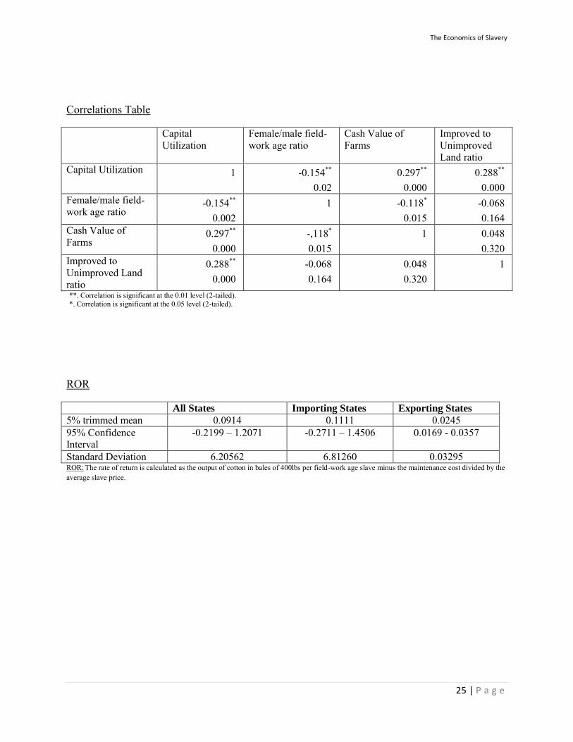
Profitability of Farms For all counties combined, the average rate of return on field-work age slaves in the

cotton production12 with maintenance costs of $15 is 9.14%13. All average ROR are 5% trimmed

means, in order to account for the large outliers of the sample.

If we look at the states independently we attain the following results. The exporting states

have an average ROR of 2.45%. The 95% confidence interval lies between 1.69% and 3.57%.

Therefore, we can conclude that the exporting states are profitable in the cotton production. For

the importing states the average ROR is 11.11%, but a large standard deviation leads to a 95%

confidence interval of -27.11% to +145.06%. It is therefore not safe to conclude that the

importing states were profitable in the cotton production. However, it needs to be noticed that

because of data constraints, the ROR is calculated assuming that all slaves in the field-work age

were occupied in the cotton production. Since this is unlikely to have been the case, the ROR

should be higher than what was attained in this analysis.

Overall, there are slightly more profitable farms in the sample of all states than

unprofitable ones, as can be derived from the pie chart below.

12

If not specified differently, the maintenance costs is assumed to be $15 per slave 13

Because of the high standard deviation due to outliers I have used the 5% trimmed mean as an estimate

Pie chart “Profitable Farms”. Measured by their ROR with a maintenance cost of $15. 239 profitable farms „1‟ and 226 unprofitable farms „0‟


15 | P a g e

The State of Texas

One example of a profitable importing state is Texas with an average ROR of 13.07%.

The 95% confidence interval lies between 8.12% and 18.03%. When the rate of return is

calculated taking into account all slaves on the plantation the numbers are as follows: the average

rate of return is 5.26%, with a 95% confidence interval that lies between 2.67% and 7.85%.

Setting the maintenance costs to the maximum estimate of $45 gives an average rate of return of

11.41% with a 95% confidence interval between 6.45% and 16.36%. The fact that probably not

all work-age slaves were working in the cotton production, makes us assume that the actual rate

of return should be above these numbers. According to the analysis, 93% of the sampled farms in

Texas are profitable in the cotton production.

Farm Size and Profitability

To find out whether large farms are more profitable than small farms, I tested the

importance of the farm‟s total land, its improved land and its cash value on the rate of return. The

results are that those farms that have a rate of return below 0, i.e. are unprofitable, average total

farm size is smaller than for those farms with a profitable ROR above 0.

5% trimmed mean Profitable Farms with a ROR>0 Unprofitable Farms with a

ROR≤0

Total Land in Acres 293.954 181.104

Improved Land in Acres 75.617 55.489

Cash value of the Farm in

Dollars

2.618.672 2.094.003

Table 1: Comparison of farm characteristics based on their profitability

Farm Size and the Number of Field-Work Age Slaves

The analysis also showed that there is a highly positive correlation of 0.739 between the

amount of improved land and the number of slaves in the field-work age. Therefore, we can

conclude that the larger farms also had more slaves in the field-work age. However, there could


16 | P a g e

not be found a significant correlation between the number of slaves in the field-work age and the

ROR. For this study, the correlation between the two variables was slightly negative (-0.066) but

had a low significance (0.258).

Farm Cotton Output and Profitability

There is a significant positive correlation of 0.166 between the amount of cotton

production and the rate of return, as can be seen in the graph below. Therefore the factors that

influence cotton production output positively are expected to also positively influence the rate of

return.

Graph 1: Scatter plot showing the relationship of the amount of cotton production and a farm‟s rate of return (ROR)

Field-Work Age Slaves in the Exporting and Importing States

We find that the slave importing states have a smaller number of slaves in the field-work

than the exporting states. On average, farms in the importing states had between 1800 and 2350

slaves, while exporting states had between 2180 and 3075 slaves in this age group. This is not in

line with the hypothesis that the Southern states adapted to the change in economic circumstances

by shifting the cotton production westwards to exploit new soil, while the states with depleted

soil concentrated on slave breeding and other non-field work.


17 | P a g e

Regression Analysis

In order to be able to get a more significant prediction the regression analysis is run on

two different dependent variables Y. The first one, Y1, is the rate of return (ROR), the second, Y2,

is the output of cotton in bales of 400lbs. It has been shown before that ROR and cotton output

are positively correlated. Each Y is analyzed for three cases: all states combined, only for the

exporting states, and only for the importing states. In total, there are 465 counties included in the

data set. The findings can be found in the table below.

All States Importing States Exporting States

Y=ROR Y=Bales of Cotton



Variables β

(sig.)

β

(sig.)

β

(sig.)

β

(sig.)

β

(sig.)

β

(sig.)

Cash Value of Farms

0.114 (0.067)

0.451 (0.000)

0.137 (0.056)

0.452 (0.000)

0.056 (0.620)

0.469 (0.000)

Female/male field-work age ratio

-0.036 (0.541)

-0.068 (0.198)

-0.003 (0.962)

0.011 (0.851)

0.729 (0.000)

0.541 (0.000)

Improved to Unimproved Land ratio

0.095 (0.170)

-0.009 (0.878)

0.104 (0.171)

-0.031 (0.652)

0.436 (0.017)

0.317 (0.038)

Capital Utilization

-0.153 (0.036)

0.053 (0.413)

-0.167 (0.04)

0.129 (0.069)

-0.352 (0.053)

-0.149 (0.320)

R Square 0.021 0.228 0.025 0.255 0.579 0.704 Table 2: Beta coefficients β, significance,

and R Square for SPSS regression analysis

Cash Value of Farms: The value of the farm in U.S. dollars Female/male field-work age ratio: The number of female slaves divided by male slaves. All slaves are in field-work age Improved to Unimproved Land ratio: Improved land divided by unimproved land. All measures are in acres Capital Utilization: Number of slaves in field-work age divided by the amount of acres of improved land ROR:

.

Bales of Cotton: Cotton output of farms measure in bales of 400lbs each

The analysis has shown that the size, i.e. value of the farm, has a positive impact on

profitability. This is consistent for the full sample of all states combined, as well as for exporting

and importing states independently. Capital Utilization has a significant negative effect on the

rate of return in each case, which is contrary to what was expected. Concerning the variable

improved land ratio, the more improved land as a percentage of unimproved land a farm has, the

higher the rate of return; meaning the variable has a positive effect on profitability. The


18 | P a g e

percentage of females in the total field-work age group has a negative effect on profitability,

except for the case where only exporting states are analyzed. There, the effect of females is

highly positive.

Overall, the most significant results and highest R square were obtained for a sample that

included only the exporting states. Furthermore, the variable Cash Value of Farms and the

variable Capital Utilization give significant results for most of the different samples under

investigation. Even though the other variables do not give us significant results, which might be

due to heteroskedasticity, the sign of the beta coefficients give an indication of the variables

effect on profitability. Throughout the analysis the regression was run every time a new state was

added to the sample. Since the sign of the beta for the most part did not change, while the

significance of the coefficient increased with the additional input of data, the results obtained can

be used as a rough estimate of a positive or negative influence.

The following hypotheses turn out to be valid with respect to this analysis: The more farm

land is made up of improved land, the higher the cotton output and profitability14. As anticipated,

female slaves do indeed lower production output and profitability compared to male slaves. Since

male slaves are physically more capable of doing hard work on the cotton fields, they can be

exploited more than female slaves. Surprisingly this situation is different if only exporting states

are included in the analysis. Female slaves then have a highly positive effect on output and

profitability. From the literature discussed in chapter 2, exporting states did indeed rely on

reproduction of slaves for trade as a way to make the states more profitable. However, in this

analysis only cotton production is included as a measure of profitability. Therefore, slave trade

could not have had an effect on profitability in this sample. Explanations for this can be data

limitations, and the influence of error terms in the data.

Capital Utilization

Contrary to what was expected is the effect of capital utilization on profitability. The

more slaves per acres of improved land a farm has, the less profitable it is in the cotton

production. This outcome makes us suggest that the maintenance costs of slaves have a larger

negative effect on the ROR than the additional cotton produced from exploiting a fixed amount of

improved land. Therefore, an increase in slaves meant that costs started to exceed benefits of

14

The negative coefficient results for Y=Bales of Cotton were ignored because of high insignificance. See Appendix A.


19 | P a g e

cotton production. This would explain why the beta coefficients for Y= ROR consistently yield a

negative beta coefficient in all samples; i.e. too many slaves were owned with respect to what

would be the optimal amount given the acres of improved land on the farm. However, the beta

coefficients were less negative or even positive for Y= Bales of Cotton. This seems logical, since

a higher number of slaves can produce more output. Therefore, the ROR seems to be a better

approximation for the dependent variable Y, as it takes into account both the benefits from

increased production but also the additional costs that accrue with owning more slaves.

Size of the Farm

There was no evidence in support of Fogel & Engerman‟s hypothesis that large farms

were not more productive than small farms. In this sample, the size, measured in the cash value

of the farm, has a positive effect on profitability. Except for the case where only exporting states

are investigated on their ROR, all cases yield highly significant positive effects of the variable

Cash Value of Farms, with coefficients ranging from 0.114 to 0.469. Thus, for any additional $1

in the cash value of the farm, profitability (ROR) is expected to increase between $0.11 and

$0.47, indicating possible internal economies of scale for the cotton farms.


20 | P a g e

Chapter 4: Conclusion

From the data analysis, it follows that cotton production was indeed profitable for some

individual farms as well as for some larger areas like the state of Texas for example. For this

particular state, the returns on slave investment were positive on average, even when maintenance

costs varied significantly. Compared to other economic activities the returns are in line with these

yields. E.g., the Railroad bond in 1860 yielded 6.2% and the New England Municipal Bond

5.2%. However, the rate of return is calculated taking into account only those slaves that are in

the field-work age. This is done because of data limitations. Calculating the rate of return

considering all slaves on the farm would require data on the contribution of those slaves that are

not in the field-work age. Furthermore, there is no data available on how many of the field-work

age slaves were actually working in the cotton production. Data on this would have allowed for a

more accurate calculation of the rate of return on cotton production, and I believe would have

changed the findings of some other states to a more profitable outcome.

In terms of the effect of the plantation‟s size and its capital utilization on profitability of

cotton production, the conclusion from the sample analysis is as follows. While larger plantations

did indeed turn out to be more profitable than smaller plantations, there also seemed to be an

indication that overall, farms owned too many slaves with respect to their availability of

improved land. I.e., profitability, measured as the ROR, decreased for any additional slave

owned, suggesting that the maintenance costs exceeded the benefits from cotton production.

As already concluded in the first chapters, the size of the sample under investigation of

profitability makes a significant difference. In the analyzed sample, individual farms and even

certain areas of a state have proven to be very profitable, while others have proven to be of the

other extreme. Thus, the large variation in the data makes it difficult to give reliable conclusions

about the whole economic system of the 19th century Southern USA. If a judgment on the

viability of slavery as an economic system has to be made on the profitability of cotton

production, it may be said that Texas, as a representative of the „new slave states‟, was indeed

very profitable in this field in 1860. It could be seen as an example for the practicability of

slavery in the cotton production, but more factors certainly have to be considered to make a

judgment on the sustainability of this system.


21 | P a g e

Further research

This research can be extended in several interesting ways. Besides taking into account

external effects on production, such as a drought, an analysis of the effect of slave trade and

hiring would let us find more concluding relationships between farms and profitability. This

would also give better conclusions about the overall flexibility of the economic system, e.g.

whether breeding for slave trade was indeed a profitable business that made up for the decrease

of plantation work in the exploited soil.

Another possible extension of this research would be to investigate the amount of

Southern slave farm‟s debt. There seems to be evidence that Southern plantations took on a lot of

debt in order to finance the high capital outlays. It makes sense to assume that the interest rate on

debt must be taken into calculations when investigating the viability or profitability of the slave

system. Little has been presented on the effect of debt on the viability of the Southern economy;

e.g. whether or not the rate of return on slavery would have been sufficient enough to cover the

interest payments on the farms debt. There was no data available that could have allowed me to

investigate this relationship myself.


22 | P a g e

Bibliography

Acemoglu, D. & Wolitzky, A. (2009). The Economics of Labor Coercion. Department of Economics Working Paper Series, MIT and CIFAR Bales, K.& Robbins, P.T. (2001). “No one shall be held in slavery or servitude”: A critical analysis of international slavery agreements and concepts of slavery. Human Rights Review. Vol. 2, No. 2. Retrieved from http://www.springerlink.com/content/jvm3jpx3fxgwk0v3/export-citation/ on March, 18 2011 Besanko, D. & Braeutigam, R.R. (2008). Microeconomics. International Student Version. 3rd edition. Hoboken, NJ: John Wiley& Sons Conrad, A.H. & Meyer, J.R. (1958). The Economics of Slavery in the Ante Bellum South. The Journal of Political Economy, Vol. LXVI, Number 2 Conrad, A.H. & Meyer, J.R. (1964). The Economics of Slavery. Chicago: ALDINE Publishing Company Ekelund, R.B. & Hebert, R.F. (1997). A History of Economic Theory And Method. 4th edition. McGraw-Hill Companies, Inc. Engerman, S. L., & Fogel, R. W. (1974). Time on the Cross: The Economics of American Negro Slavery. London: Wildwood House Limited Engerman, S. L., & Fogel, R. W. (1970). The Relative Efficiency of Slavery: A Comparison of Northern and Southern Agriculture in 1860. Preliminary report of a research project supported by the National Science Foundation under grant numbers GS-3262, GS-27143, and GS-27262. Fenoaltea, S. (1984). Slavery in Comparative Perspective: A Model. Journal of Economic His- tory, 44, pp. 635-638. Fitzhugh, George. (1857). Cannibals All! Or, Slaves Without Masters. Bedford, MA: Applewood Books. 2008 edition. Fleischman, R.K. & Tyson, T.N. (2002). Accounting in service to racism: monetizing slave property in the Antebellum South. Department of Accountancy, John Caroll University and Department of Accounting, St. John Fisher College. Elsevier, Critical Perspectives on Accounting 15 (2004) 376-399 Gallaway, L.E., Klingman, D.C., Vedder, R.K. (date unknown). The Profitability of Ante Bellum Agriculture in the Cotton Belt: Some New Evidence. Atlantic Economic Journal. Volume 2, Number 2

http://www.springerlink.com/content/jvm3jpx3fxgwk0v3/export-citation/

http://www.springerlink.com/content/jvm3jpx3fxgwk0v3/export-citation/

http://www.springerlink.com/content/0197-4254/

http://www.springerlink.com/content/0197-4254/2/2/

http://www.springerlink.com/content/0197-4254/2/2/


23 | P a g e

Giles, W.H. (2006). Slavery and the American Economy. Retrieved from http://www.nathanielturner.com/slaveryandtheamericaneconomy.htm on March 1st, 2011 Kettell, T.P. (1860). Southern Wealth and Northern Profit. New York: George W. & John A. Wood Nunn, N. (2007). Slavery, Inequality, and Economic Development in the Americas: An Examination of the Engerman-Sokoloff Hypothesis. Department of Economics, Harvard University and NBER Post, C. (2003). Plantation Slavery and Economic Development in the Antebellum Southern United States. Journal of Agrarian Change. Vol. 3. Pp. 289-332

Ramsdell, C. W. (1929). The Natural Limits of Slavery Expansion. The Southwestern Historical Quarterly. Vol. XXXIII. No. 2

Spangenberg, J.H. (2005). Economic sustainability of the economy: concepts and indicators. Int. J. Sustainable Development, Vol. 8, Nos. 1/2, 2005 47. Retrieved from http://www.environmental-expert.com/Files/6471/articles/6328/f211108463951127.pdf on March 4th, 2011 Stein, S.H. (2007). A Beginner's Guide to the Solow Model. Journal of Economic Education, 38(2), 187-189,191-193. Retrieved March 18, 2011, from ABI/INFORM Global. (Document ID: 1312838871). Vedder, R.K. (1975). The Slave Exploitation (Expropriation) Rate. Explorations in Economic History 12, 453-457. Ohio University Woodman, H.D. (1963). The Profitability of Slavery: A Historical Perennial. The Journal of Southern History, Vol. 29, No. 3, pp. 303-325.


24 | P a g e

Appendix A

States and Number of Counties included in the Sample

Slave Importing States

Alabama Louisiana Mississippi Texas Total Importing

Counties 52 48 60 151 311

Slave Exporting States

South Carolina Virginia Maryland Total Exporting Counties 31 124 0* 155 *Maryland was excluded from the sample because of missing data on cotton output

Regression Analysis





Variables β

(sig.)

β

(sig.)

β

(sig.)

β

(sig.)

β

(sig.)

β

(sig.)

Cash Value of Farms

0.114 (0.067)

0.451 (0.000)

0.137 (0.056)

0.452 (0.000)

0.056 (0.620)

0.469 (0.000)


-0.036 (0.541)

-0.068 (0.198)

-0.003 (0.962)

0.011 (0.851)

0.729 (0.000)

0.541 (0.000)


0.095 (0.170)

-0.009 (0.878)

0.104 (0.171)

-0.031 (0.652)

0.436 (0.017)

0.317 (0.038)

Capital Utilization

-0.153 (0.036)

0.053 (0.413)

-0.167 (0.04)

0.129 (0.069)

-0.352 (0.053)

-0.149 (0.320)

R Square 0.021 0.228 0.025 0.255 0.579 0.704 Cash Value of Farms: The value of the farm in U.S. dollars Female/male field-work age ratio: The number of female slaves divided by male slaves. All slaves are in field-work age Improved to Unimproved Land ratio: Improved land divided by unimproved land. All measures are in acres Capital Utilization: Number of slaves in field-work age divided by the amount of acres of improved land


25 | P a g e

Correlations Table

Capital Utilization


Cash Value of Farms


Capital Utilization 1

-0.154**

0.02 0.297**

0.000 0.288**

0.000 Female/male field-work age ratio

-0.154**

0.002 1 -0.118*

0.015 -0.068 0.164

Cash Value of Farms

0.297**

0.000 -,118*

0.015 1

0.048 0.320


0.288**

0.000 -0.068 0.164

0.048 0.320

1

**. Correlation is significant at the 0.01 level (2-tailed). *. Correlation is significant at the 0.05 level (2-tailed).

ROR


5% trimmed mean 0.0914 0.1111 0.0245 95% Confidence Interval

-0.2199 – 1.2071 -0.2711 – 1.4506 0.0169 - 0.0357

Standard Deviation 6.20562 6.81260 0.03295 ROR: The rate of return is calculated as the output of cotton in bales of 400lbs per field-work age slave minus the maintenance cost divided by the average slave price.

the economics of slavery - tilburg university

Documents