The Effect of Capital Market Characteristics

on the Value of Start-Up Firms∗

Roman Inderst† Holger M. Müller‡

February 2003

∗We are particularly grateful to an anonymous referee for thoughtful comments and suggestions. Thanks also

to Patrick Bolton, Mike Burkart, Paul Gompers, Denis Gromb, Thomas Hellmann, Pete Kyle, Enrico Perotti, Per

Strömberg, Elu von Thadden, Masako Ueda, Jeff Wurgler, and seminar participants at Dartmouth, Amsterdam,

Humboldt, Mannheim, Stockholm School of Economics, Tilburg, the Financial Markets Conference on Venture Capital

and Technology: What’s Next? in Sea Island, GA (2002), the Annual Meeting of the European Finance Association in

Berlin (2002), the Five Star Conference on Research in Finance at NYU (2001), the workshop on Strategic Interactions

in Relationship Finance: Bank Lending and Venture Capital at LSE (2001), the workshop on Finance for the XXI

Century in Amsterdam (2001), and the European Summer Symposium in Financial Markets (ESSFM) in Gerzensee

(2001) for helpful comments. Earlier versions of this paper circulated under the titles “Competition and Efficiency in

the Market for Venture Capital” and “Venture Capital Contracts and Market Structure.”

†London School of Economics & CEPR. Address: Department of Economics & Department of Accounting and

Finance, London School of Economics, Houghton Street, London WC2A 2AE. Email: r.inderst@lse.ac.uk.

‡New York University & CEPR. Address: Department of Finance, Stern School of Business, New York University,

44 West Fourth Street, Suite 9-190, New York, NY 10012-1126. Email: hmueller@stern.nyu.edu.

1

Abstract

We show how the value, valuation, and success probability of start-ups depend on characteristics

of the capital market. Market characteristics such as the return on investments, entry costs, and

capital market transparency affect the relative supply and demand for capital, and thus the relative

bargaining power of entrepreneurs and venture capitalists. Relative bargaining power, in turn,

determines ownership shares and incentives in start-up firms. In characterizing the short- and

long-run dynamics of the venture capital market, the model sheds light on the Internet boom and

bust periods. The model is consistent with available empirical evidence and provides many novel

empirical predictions.

2

1 Introduction

The venture capital industry is highly cyclical, with periodic changes in supply and demand condi-

tions (Gompers and Lerner (1999), Lerner (2002)). Between the fourth quarters of 2000 and 2001,

for instance, total funds raised dropped by more than 80 percent. In this paper we ask whether,

and how, such variations in the capital supply affect the structure of venture capital deals.

Our theory is based on two intuitive building blocks. The first is a model of contracting and

bargaining in start-up firms. Building on Sahlman (1990), Kaplan and Strömberg (2002b), and

Hellmann and Puri (2001), we model the relationship between the entrepreneur and venture cap-

italist as a double-sided incentive problem: A greater fraction of the firm owned by the venture

capitalist improves the venture capitalist’s incentives but dulls the entrepreneur’s incentives. Effi-

ciency requires balancing the two incentive problems or, equivalently, balancing ownership shares.

Actual ownership shares, however, are determined by bargaining, and thus by the relative strengths

of the entrepreneur’s and venture capitalist’s outside options.

The second building block is a search model linking outside options to the relative magnitude of

supply and demand for venture capital. An increase in capital supply, for example, makes it easier

for an entrepreneur to obtain financing, thereby increasing his outside option vis-a-vis a venture

capitalist. The supply of capital, in turn, is linked to primitive market characteristics such as the

profitability of investments, entry costs, and capital market transparency.

The end result is an equilibrium model in which capital market characteristics affect the relative

supply and demand for capital, which in turn affect ownership shares, which in turn affect the value,

valuation, and success probability of start-up firms.

The core of our analysis is a characterization of the short- and long-run dynamics of the venture

capital industry. In the short run, the supply and demand for capital are fixed. In the long run,

capital inflows respond to changes in market conditions, which makes capital market competition en-

dogenous. For instance, our model predicts that an increase in the return on investments–whether

genuine or perceived–leads to new entry and a long-run increase in capital market competition,

coupled with a rise in valuations and a decline in venture capitalists’ ownership shares. A decrease

in profitability, on the other hand, leads to exit by investors, a drop in valuations, and better deal

terms for those venture capitalists remaining in the market.

While stylized, our model appears to provide a useful picture of the boom and bust of the

Internet. As this industry emerged, it seems that winners materialized more quickly than losers,

which possibly caused capital providers to overestimate the true shock to investment profitability.

As more and more firms failed, the market corrected its initial assessment and adjusted its estimate

3

downward. Boom and bust thus correspond to an increase and decrease in the (true or perceived)

return on investments, respectively.

We also examine the equilibrium effects of changes in entry costs and capital market trans-

parency. Such changes affect outside options either directly or through their effect on competition.

Our model predicts that an increase in transparency improves the value created in start-ups, while

a reduction in entry costs may destroy value if the capital supply is already at a high level. Finally,

capital market competition not only affects the incentives after, but also prior to the formation of

a new venture. In an extension of the model we show that venture capitalists are more likely to

screen projects in down markets when competition among capital providers is weak, and less likely

in hot markets when competition is strong.

Our model of search and matching contrasts with traditional venture capital contracting models,

which consider an isolated setting with one entrepreneur and one venture capitalist at a time. In

the background of these models is a competitive capital market in which entrepreneurs capture all

the rents. In a world with many venture capitalists and many entrepreneurs, however, it is not clear

why entrepreneurs should capture all the rents. On the contrary, anecdotal evidence suggests that

the power to appropriate rents shifts back and forth between entrepreneurs and investors depending

on which side is currently in short supply.1

A central tenet of our model is that changes in capital market competition and relative bargaining

powers translate into changes in ownership shares. Gompers and Lerner (2000), for instance, find

a strong positive relation between the pre-money valuation of new ventures and capital inflows,

suggesting that “increases in the supply of venture capital may result in greater competition to

finance companies and rising valuations.” Unless the size of venture capital investments increases

proportionately, a rise in valuations implies a greater ownership share for entrepreneurs and a smaller

share for venture capitalists.

Another central tenet of our model is the link between ownership shares and incentives. Kaplan

and Strömberg (2002b), for instance, find that equity incentives increase the likelihood that venture

capitalists provide value-adding support activities. In a similar vein, unfavorable deal terms (from

the perspective of entrepreneurs) in the recent down market have caused concerns that the incentives

of entrepreneurs might have suffered: “The terms of current venture financings can be such that

1The following statement compares the height of the internet bubble when capital supply was abundant to the

aftermath when capital became relatively more scarce: “If you went into a [...] start-up three to six months ago, you

almost certainly got a very bad deal. Companies could ask for anything they wanted [in terms of valuation]. Now

entrepreneurs are much more realistic” (Financial Times (2001)). Similarly, Bartlett (2001b) argues that the burst of

the internet bubble brought about “changes in deal terms [...] all of which are designed to enhance returns and the

quantum of control enhoyed by nervous investors.”

4

founders may well lose interest. [...] They start plotting their next career move, perhaps with a

competitor, from the date the deal is closed. In short, the VCs, while putting in place extremely

favorable terms from their point of view, face the possibility of shooting themselves in the feet.”

(Bartlett (2001a)).

The main difference between our model and traditional venture capital contracting models is

that in our model the focus is not on contracting, but on the richer interaction between contracting,

bargaining, and the capital market environment. Capital market characteristics determine outside

options, which in turn determine relative bargaining powers, which in turn determine contracts and

incentives. Michelacci and Suarez (2002) also have a search model of start-up financing. Unlike

this paper Michelacci and Suarez do not consider incentive contracts or inefficiencies arising from

an imbalance of ownership shares. Rather, they focus on search inefficiencies, using an insight

from the search literature that entry creates externalities for the matching chances of other market

participants. Related is also Legros and Newman (2000), who study the relation between the

distribution of liquidity in the economy and the incentives of agents to engage in joint production.

Unlike this paper there is no investment to be financed. Liqudity is used only to attract holders of

complementary assets and to facilitate the trading of control rights.

The rest of the paper is organized as follows. Section 2 presents the model. Section 3 char-

acterizes the equilibrium for the case where capital market competition is exogenous. Section 4

endogenizes the level of capital market competition and studies the effects of a shift in investment

profitability, entry costs, and capital market transparency. Section 5 discusses welfare and policy

implications. Section 6 considers robustness issues. Section 7 examines the incentives of venture

capitalists to screen projects. Section 8 summarizes the empirical implications and compares them

to the available evidence. Section 9 concludes. All proofs are in the Appendix.

2 The Model

The model has two building blocks: (i) a model of contracting and bargaining in start-ups, and (ii)

an equilibrium model of search. We first derive the bargaining frontier characterizing the utilities

of the entrepreneur and venture capitalist for all Pareto optimal contracts. We then derive the

bargaining solution, which determines a point (i.e., contract) on the bargaining frontier. In the

bargaining we take the entrepreneur’s and venture capitalist’s outside options as given. We finally

embed the bargaining problem in a search market, thereby endogenizing outside options as a function

of capital market competition. The level of capital market competition, in turn, is taken as given.

It will be endogenized in Section 4 when we introduce free entry of capital.

5

2.1 Financial Contracting

A penniless entrepreneur has a project requiring an investment I > 0. Financing is provided by a

venture capitalist. The project payoff is Xl ≥ 0 with probability 1− p and Xh > I with probabilityp. The success probability p = p (e, a) depends on the entrepreneur’s and venture capitalist’s non-

contractible efforts e ∈ [0, 1] and a ∈ [0, 1]. Effort costs are denoted by c (e) and g (a), respectively,and are strictly convex. All agents are risk neutral.

In the base model (Sections 2-5) we assume that Xl = 0. With Xl = 0 a financial contract

between the venture capitalist and entrepreneur is fully characterized by a sharing rule s ∈ [0, 1] .We frequently refer to s as the venture capitalist’s output, or ownership, share. The case where

Xl is positive is considered in Section 6. In that section we also consider the possibility that the

venture capitalist pays the entrepreneur a wage.

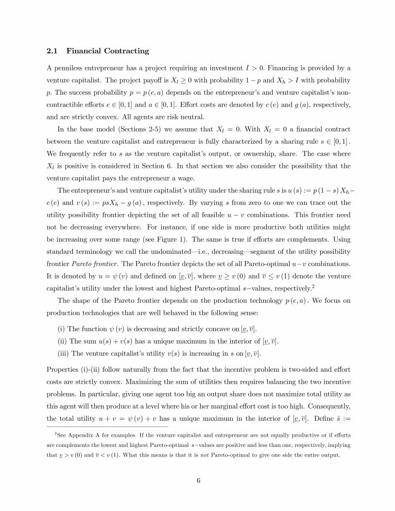
The entrepreneur’s and venture capitalist’s utility under the sharing rule s is u (s) := p (1− s)Xh−c (e) and v (s) := psXh − g (a) , respectively. By varying s from zero to one we can trace out the

utility possibility frontier depicting the set of all feasible u − v combinations. This frontier neednot be decreasing everywhere. For instance, if one side is more productive both utilities might

be increasing over some range (see Figure 1). The same is true if efforts are complements. Using

standard terminology we call the undominated–i.e., decreasing–segment of the utility possibility

frontier Pareto frontier. The Pareto frontier depicts the set of all Pareto-optimal u−v combinations.It is denoted by u = ψ (v) and defined on [v, v], where v ≥ v (0) and v ≤ v (1) denote the venturecapitalist’s utility under the lowest and highest Pareto-optimal s−values, respectively.2

The shape of the Pareto frontier depends on the production technology p (e, a) . We focus on

production technologies that are well behaved in the following sense:

(i) The function ψ (v) is decreasing and strictly concave on [v, v].

(ii) The sum u(s) + v(s) has a unique maximum in the interior of [v, v].

(iii) The venture capitalist’s utility v(s) is increasing in s on [v, v].

Properties (i)-(ii) follow naturally from the fact that the incentive problem is two-sided and effort

costs are strictly convex. Maximizing the sum of utilities then requires balancing the two incentive

problems. In particular, giving one agent too big an output share does not maximize total utility as

this agent will then produce at a level where his or her marginal effort cost is too high. Consequently,

the total utility u + v = ψ (v) + v has a unique maximum in the interior of [v, v]. Define s :=

2See Appendix A for examples. If the venture capitalist and entrepreneur are not equally productive or if efforts

are complements the lowest and highest Pareto-optimal s−values are positive and less than one, respectively, implyingthat v > v (0) and v < v (1). What this means is that it is not Pareto-optimal to give one side the entire output.

6

argmax[u(s)+v(s)], v := v(s), and u := u(v(s)).We frequently refer to s as the second-best sharing

rule. Evidently, it holds that ψ0 (v) = −1, i.e., if total utility is maximized the Pareto frontier hasa slope of minus one. The third property states that the venture capitalist’s utility is increasing in

her output share. This automatically implies that u0(s) > 0. This assumption is needed to rule out

situations where a value of ψ (v) is associated with more than one s−value.All three assumptions are innocuous and satisfied by many production technologies. In Appendix

A we give two examples of technologies satisfying (i)-(iii) used in the venture capital literature: the

linear technology p (e, a) = γa + (1 − γ)e used in, e.g., Casamatta (2000), and the Cobb-Douglastechnology p (e, a) = aγe1−γ used in, e.g., Repullo and Suarez (2000). Under the linear technology

the two efforts are substitutes while under the Cobb-Douglas technology they are complements. To

make the problem nontrivial we assume that v > I, i.e., the joint-surplus maximizing allocation is

sufficiently profitable to allow the venture capitalist to break even.

The entrepreneur’s and venture capitalist’s deal utilities are U(s) := u(s) and V (s) := v(s)− I,respectively. In Section 6 we extend the concept of deal utilities by incorporating the safe payoff Xl

and wage payments. Hence the “effort-related utilities” u(s) and v(s) are merely one element of the

agents’ overall deal utilities. The set of all Pareto-optimal U − V combinations is called bargainingfrontier and denoted by Ψ(V ). In the base model where Xl = 0 the bargaining frontier is obtained

from the Pareto frontier by shifting ψ (v) to the left by I, implying that Ψ(V ) := ψ(V + I). In

Section 6 where Xl > 0 the construction of the bargaining frontier is more complicated. The domain

of the bargaining frontier is [V , V ], where V := max {v − I, 0} and V := v − I.3Figure 1 depicts the utility possibility frontier characterizing all feasible u−v combinations, the

Pareto frontier characterizing all Pareto-optimal u − v combinations, and the bargaining frontiercharacterizing all Pareto-optimal U − V combinations for the Cobb-Douglas technology.

Figure 1 here

2.2 Bargaining

It is reasonable to assume that when bargaining over a contract the entrepreneur and venture

capitalist choose a contract that is Pareto efficient. Bargaining thus corresponds to choosing a

utility pair (V,U) on the bargaining frontier. If the bargaining breaks down the entrepreneur and

venture capitalist realize their outside options Uo and V o, respectively. For the moment we take

these outside options as given. They are endogenized in Section 4 as a function of capital supply and

3As the venture capitalist and entrepreneur never bargain to a point where the venture capitalist’s utility is negative

the nonnegativity constraint max {v − I, 0} involves no loss of generality.

7

demand. As a bargaining concept we use the generalized Nash bargaining solution. Accordingly, the

bargaining outcome consists of utilities U = Ψ(V ) ≥ Uo and V ≥ V o maximizing the Nash product[V − V o]η [Ψ(V )− Uo]1−η, where η ∈ (0, 1) . For expositional convenience define β := η/(1− η).

As the bargaining frontier is strictly concave the bargaining problem has a unique solution.

In the Appendix (Proof of Proposition 1) we show that this solution lies in the interior of [V , V ].

Denote the bargaining solution by¡V d, Ud

¢, where Ud := Ψ(V d). The superscript indicates that V d

and Ud are the equilibrium utilities realized in a deal. Maximizing the Nash product with respect

to V we obtain the following result.

Lemma 1. The equilibrium deal utilities V d and Ud are uniquely determined by

β = −Ψ0(V d) V d − V oΨ(V d)− Uo (1)

and Ud = Ψ(V d).

Accordingly, the venture capitalist’s deal utility is increasing in her own and decreasing in

the entrepreneur’s outside option. The opposite is true for the entrepreneur. As is well known, the

axiomatic Nash bargaining solution can be derived as the limit of a non-cooperative bargaining game

where the two parties bargain with an open time horizon under the risk of breakdown (Binmore,

Rubinstein, and Wolinsky (1986)). It is worth noting that our results do not depend on the specifics

of the Nash bargaining solution. All that is needed is that an agent’s deal utility is positively related

to his own and negatively related to his counterparty’s outside option. Any bargaining concept with

this feature yields analogous results.

2.3 Search

To endogenize outside options we embed the bargaining problem in a market environment. We

consider a stationary search market populated by entrepreneurs and venture capitalists.4 The

measure of entrepreneurs and venture capitalists in the market is Me and Mv, respectively. A key

variable is the ratio of venture capitalists to entrepreneurs, or degree of capital market competition,

Mv/Me =: θ. A high value of θ indicates that the capital market is highly competitive. Each

venture capitalist has capital k, which implies she can finance at most one project. All our results

extend to the case where venture capitalists can finance finitely many projects. As each venture

capitalist has a fixed amount of capital the ratio Mv/Me =: θ also indicates the relative magnitude

of capital supply to demand. Finally, time is continuous and both sides discount future utilities with

4Our search model is known as Diamond-Mortensen-Pissarides model (e.g., Pissarides (1990)).

8

the interest rate r > 0.5

The measure of deals, or matches, per unit of time is given by the matching function x(Me,Mv).

From the viewpoint of a venture capitalist the (Poisson) arrival rate of a deal is x(Me,Mv)/Mv,

while the entrepreneur’s deal arrival rate is x(Me,Mv)/Me.We assume that the matching function

exhibits constant returns to scale. One implication of this is that deal arrival rates depend solely on

the degree of capital market competition θ. (See Section 6.4.) In particular, the venture capitalist’s

deal arrival rate is x(Me,Mv)/Mv := qv(θ), which is decreasing in θ with limθ→0 qv(θ) = ∞ and

limθ→∞ qv(θ) = 0. Hence a venture capitalist is more likely to meet an entrepreneur in a given

time interval if the ratio of venture capitalists to entrepreneurs is low. Given that the measure of

deals per unit of time is Mvqv(θ) the entrepreneur’s deal arrival rate is θqv(θ) =: qe(θ), which is an

increasing function of θ. Hence an entrepreneur is more likely to meet a venture capitalist if the

ratio of venture capitalists to entrepreneurs is high.

If the search is successful the venture capitalist and entrepreneur bargain over a contract. The

outside options in the bargaining Uo and V o are the utilities from re-entering the market and

searching anew. Given that the market is stationary the utility from re-entering the market equals

the utility from being in the market in the first place. Hence the superscript “o” has a double

meaning: it indicates that Uo and V o denote the outside options in the bargaining as well as the

overall utilities from being in the market. The entrepreneur’s and venture capitalist’s outside options

are given by the asset value equations

rUo = qe(θ)(Ud −Uo) (2)

and

rV o = qv(θ)(Vd − V o), (3)

respectively.6

For an intuitive derivation of these equations consider the entrepreneur’s outside option. The

Poisson arrival rate of a deal for the entrepreneur is qe(θ). The probability that a deal occurs in

the next small time interval ∆ is thus qe(θ)∆. With probability 1− qe(θ)∆ no deal occurs and the

entrepreneur continues his search. The expected discounted utility from searching is therefore

Uo = qe(θ)∆ exp (−r∆)Ud + (1− qe(θ)∆) exp (−r∆)Uo.5Frictions are thus expressed as costs of delay. The model can be easily extended to include direct search costs.

For convenience we assume that both sides use the same discount rate.

6We thus implicitly assume that the venture capitalist can invest her funds I at the interest rate r while searching

for an investment opportunity.

9

Solving for Uo and letting ∆→ 0 we have

Uo =qe(θ)

qe(θ) + rUd. (4)

Rearranging yields (2). The derivation of (3) is analogous. Equation (4) nicely illustrates the

relation between the entrepreneur’s overall utility from being in the market Uo and his deal utility

Ud. The overall utility is the discounted expected utility from the deal or, alternatively, the utility

from the deal minus the expected cost of delay, implying that Uo < Ud. By (4) the difference

between Ud and Uo is smaller the lower the discount rate r and the greater the speed of matching

qe(θ).

If the entrepreneur and venture capitalist reach an agreement they leave the market. Stationarity

requires that the inflow of venture capitalists and entrepreneurs matches their outflow. Denote the

measure of entrepreneurs and venture capitalists arriving in the market per unit of time by me and

mv, respectively. The market is stationary if qv(θ)Mv = mv and qe(θ)Me = me. As stationarity can

always be accomplished by scaling flows and stocks accordingly, the market is fully characterized

by the degree of capital market competition θ.

2.4 Equilibrium Conditions

The following definition summarizes the equilibrium conditions.

Capital Market Equilibrium. An equilibrium is characterized by three conditions.

(i) The deal utilities¡V d, Ud

¢maximize the Nash product [V − V o]η [Ψ(V )− Uo]1−η.

(ii) The outside options (V o, Uo) satisfy the asset value equations (2)—(3).

(iii) The flows and stocks of entrepreneurs and venture capitalists, (me,mv) and (Me,Mv) , satisfy

the stationarity conditions qv(θ)Mv = mv and qe(θ)Me = me.

The equilibrium is the solution to a system of four equations: the equation characterizing the

bargaining solution (1), the asset value equations (2) and (3), and the identity Ud = Ψ(V d). In

the bargaining solution the deal utilities V d and Ud are a function of the outside options V o and

Uo. Conversely, in the asset value equations the outside options are a function of the deal utilities.

Inserting (2)—(3) into (1) we obtain

βr + qv(θ)

r + qe(θ)= −Ψ0(V d) V d

Ψ(V d), (5)

which implicitly defines the equilibrium value of V d as a function of θ. Inserting the solution in

Ud = Ψ(V d) yields the equilibrium value of Ud, while inserting V d and Ud in the asset value

equations (2)—(3) yields the equilibrium values of V o and Uo.

10

3 Value Creation in Start-Ups

3.1 Output Shares, Individual Utilities, and Total Value

The following proposition characterizes how individual utilities and the value created in start-ups

depend on the level of capital market competition.

Proposition 1. For each level of capital market competition θ there exists a unique equilib-

rium. The venture capitalist’s output share s, her deal utility V d, and her overall utility V o are all

decreasing in θ. The reverse is true for the entrepreneur. The total value created in the start-up

V d + Ud is first increasing and then decreasing in θ.

Deal utilities and overall utilities move in the same direction. Consider, for instance, the entre-

preneur. An increase in capital market competition makes it easier for the entrepreneur to find a

counterparty, which reduces his cost of delay. The entrepreneur’s outside option Uo thus increases

(and the venture capitalist’s outside option V o decreases), which implies the bargaining outcome

shifts in favor of the entrepreneur. As a result the entrepreneur’s deal utility Ud increases and the

venture capitalist’s deal utility decreases, which implies that s decreases. The increase in Ud feeds

back into the search market dynamics. As the utility from doing a deal goes up searching for a deal

becomes more valuable. The overall utility Uo therefore increases again, and so on. This process

continues until a steady-state equilibrium is reached. An increase in θ thus corresponds to a move

along the bargaining frontier from the right to the left.

The rest follows from the construction of the bargaining frontier. As we move from the right

to the left the venture capitalist’s output share s decreases. This weakens the venture capitalist’s

incentives and improves the entrepreneur’s incentives. The total effect depends on the current value

of s. When s > s a reduction in s increases the total value created V d + Ud. When s = s the total

value is maximized. Finally, when s < s a reduction in s decreases the total value.

3.2 Pre- and Post-Money Valuation

A measure of the firm’s value commonly used in the industry is the post-money valuation. The post-

money valuation is an implied value calculated on the basis of the venture capitalist’s ownership

share. If the venture capitalist pays an amount I in return for a share s the post-money valuation

is Λ = I/s. The pre-money valuation is Γ = Λ − I = I(1 − s)/s. The post-money valuation iscommonly used as a measure of the firm’s present value while the pre-money valuation is used as

a measure of the firm’s NPV. By Proposition 1 the venture capitalist’s ownership share is inversely

related to the degree of capital market competition. This gives the following result.

11

Proposition 2. The pre- and post-money valuation are both increasing in level of capital market

competition.

Hellmann (2002) argues that the notion of valuation used in the industry is potentially flawed.

Our model supports this critique. First, the concept of post-money valuation is based on the idea

that a venture capitalist just breaks even on her investment: sΛ = I. By contrast, our model

shows that in a competitive market with frictions and moral hazard venture capitalists gets back

strictly more than they invest. On the one hand, venture capitalists needs to be compensated

for their effort costs. Moreover–and more importantly–depending on the level of capital market

competition venture capitalists earn a bargaining premium. Specifically, in our model the venture

capitalist’s deal utility is V d = spXh − g (a) − I > V o, which is strictly positive. Hence the valueof the venture capitalist’s stake, spXh, strictly exceeds her combined effort and investment costs

g (a) + I.

Our model also suggests that the post-money valuation is a poor indicator of firm value. Holding

I fixed, the valuation varies mechanically with the venture capitalist’s ownership share s. The

ownership share, however, is determined by bargaining. If anything, valuations thus reflect relative

bargaining powers. The notion that valuations measure relative bargaining powers is consistent

with empirical evidence by Gompers and Lerner (2000) showing a positive relation between the

pre-money valuation and capital market competition.7

With additional assumptions it is possible to say something more about the difference between

value and valuation. Suppose the lowest and highest Pareto-optimal s−values are close to zero andone, respectively.8 From the definition of Γ and the monotonic relation between s and θ it follows

that for low θ the pre-money valuation is close to zero while for high θ it becomes arbitrarily large.

The total value created in the start-up, V d + Ud, on the other hand, is first increasing and then

decreasing in θ. Moreover, it is strictly bounded away from zero for all θ.9 Together, this implies

that the pre-money valuation understates the total value created in the start-up if competition is

low and overstates it if competition is high.

7Bartlett (2002) also suggests that valuation is an indicator of bargaining power rather than firm value: “The

discussion starts out with the issue of valuation. The entrepreneur and his or her advisors lay on the table a number,

based on art as much as science, and suggest that the venture capitalist agree with it [...] The price, in other words,

is usually left to naked negotiations between the buy and the sell side.”

8This is consistent with a production function where efforts are close substitutes and productivity levels are similar.

Incidentally, s = 0 is not feasible as the venture capitalist then does not break even.

9This follows from the fact that the bargaining frontier is decreasing. Hence if θ takes on extreme values–implying

that the deal utility of one side is minimal–the deal utility of the other side is maximal.

12

3.3 Market Value and Success Probability

The total value V d + Ud takes into account both investment and effort costs. By contrast, the

interim market value pXh is the expected value of the firm after effort and investment costs have

been sunk but before cash flows are realized. It is what the entrepreneur and venture capitalist

could hope to receive if the firm was sold at an interim date. As Xh is a constant the functional

behavior of pXh is identical to that of the success probability p (e, a) .

Unlike the total value the relation between p (e, a) and s or θ is not necessarily characterized

by an inverted U-shape. Precisely, the relation depends on whether the venture capitalist’s and

entrepreneur’s efforts are complements or substitutes. To explore this issue we consider the CES

production technology p (e, a) = [γaκ + (1 − γ)eκ ] 1κ , where κ ≤ 1 and γ ∈ (0, 1) . The parameterκ measures the degree of complementarity between the two efforts. If κ = 1 efforts are perfect

substitutes while if κ < 1 efforts are complements. To obtain a closed-form solution we assume

quadratic effort costs c (e) := e2/2αe and g (a) := a2/2αv, respectively.

Consider first the case where efforts are complements. It is straightforward to show that the

success probability is first increasing and then decreasing in s with interior maximum

s∗p :=1

1 + ϕ, where ϕ :=

"µαeαv

¶κ2µ1− γγ

¶# 11−κ

.

Given the inverse relation between s and the level of capital market competition θ an increase in

θ thus has a positive effect on the success probability and market value if θ is low and a negative

effect if θ is high. Note that the value of s maximizing the success probability or market value is

generally not the same as the value of s maximizing the total value V d+Ud. The reason is that the

total value includes effort costs while the market value or success probability do not.

If efforts are perfect substitutes the success probability and market value are increasing in s

(and thus decreasing in θ) if the venture capitalist is more productive (ϕ < 1) and decreasing in

s if the entrepreneur is more productive (ϕ > 1). The case where efforts are perfect substitutes is

a knife-edged case, however, and less likely to be empirically relevant. The following proposition

summarizes our results.

Proposition 3. Unless efforts are perfect substitutes the market value and success probability

are first increasing and then decreasing in the level of capital market competition.

4 Industry Dynamics

In the preceding section we have taken the supply and demand for capital–and hence the degree

of capital market competition–as exogenously given. We believe this is a useful characterization

13

of the short run: “The skills needed for successful venture capital investing are difficult and time-

consuming to acquire. During periods when the supply or demand for venture capital has shifted,

adjustments in the number of venture capitalists and venture capital organizations appear to take

place very slowly” (Gompers and Lerner (1999)).

In the long run the supply of capital is endogenous. We now endogenize the entry decision of

venture capitalists, thereby endogenizing the capital supply and level of capital market competition.

4.1 Endogenous Entry of Venture Capitalists

We take as given the flow of new ideas, or projects, that are continuously created in the economy.

We thus implicitly assume that the supply of capital adjusts more quickly to exogenous shocks than

the supply of new ideas. In Section 6.3 we show that our results extend if both the supply and

demand for venture capital are endogenous.

Each idea is associated with an entrepreneur and cannot be traded. We normalize the flow of

new ideas such that the mass me = 1 of ideas is created in the market during one unit of time.

The inflow of capital is determined by a zero-profit constraint. We assume that a venture capitalist

entering the market incurs a fixed cost k > 0. Like any business, setting up a venture capital firm

involves fixed costs. There are costs of setting up a legal structure, hiring experts and support staff,

and building a network of lawyers, investment bankers, and clients. However, costs also arise from

the fact that during the duration of the venture fund the capital committed to the fund cannot

be invested in long-term, illiquid assets. The foregone illiquidity premium is a fixed cost as it is

incurred regardless of whether the committed capital is invested or not. (One way to think of this is

that in order to provide the capital the limited partners must free resources from other, potentially

more profitable long-term investments.)

The first type of cost is borne by the general partners while the second type is borne by the

limited partners. From the perspective of our model this is of secondary order, however, since we

treat general and limited partners as a homogeneous entity. Finally, with the exception of Section

4.4 the size of k is irrelevant for our analysis. Hence we are perfectly comfortable with the notion

that entry costs are small–as long as they are positive.

Free entry implies that the utility from entering the market V o must equal the entry cost k. One

implication of this is that V o > 0 : to recoup entry costs a venture capitalist must earn a positive

utility in the market. The equilibrium conditions are the same as before, except that now me = 1

and V o = k. We conclude by showing that there is a one-to-one relation between k and θ.

Proposition 4. For each level of entry costs there exists a unique equilibrium associated with

a unique level of capital market competition.

14

4.2 Changes in Investment Profitability

One potential explanation for the massive entry of venture funds in the mid 1990s is the expectation

of above average returns. To the extent that the Internet caused a genuine and persistent increase

in productivity these expectations might have been justified. To some extent, however, it appears

the market overreacted. For instance, winners typically tend to materialize quicker than losers.

It is possible that the market viewed early winners such as ebay or Amazon as representative of

the entire industry, thereby underestimating the true default risk of dot.coms (Hellmann and Puri

(2002)). Second, the market might have not fully taken into account the impact of competition

on the survival chances of firms. Even if sector growth had been predicted correctly, it seems that

some firms were valued as if they were the sole competitor in the sector (Lerner (2002)).

In the following we examine the consequences of changes in investment opportunities caused,

e.g., by technological innovations such as the Internet. From the perspective of our model such

changes can be either real or perceived. All we require is that investors and entrepreneurs have the

same perception, i.e., they have homogeneous beliefs. Hence our model applies equally to situations

in which entry occurs following a genuine increase in profitability as well as situations in which

entry occurs because everyone overestimates the true increase in profitability.

Expansion of the Pareto (and Bargaining) Frontier

Given that Xl = 0 a change in investment profitability translates into a change in Xh. An

increase in Xh shifts the Pareto frontier outward while a decrease in Xh shifts it inward. We

assume that along the Pareto frontier utilities are separable of the form u(Xh, s) = χ(Xh)ωe(s) and

v(Xh, s) = χ(Xh)ωv(s), where χ(Xh) and ωv(s) are increasing functions and ωe(s) is a decreasing

function. Both the linear technology p (e, a) = γa + (1 − γ)e and the Cobb-Douglas technologyp (e, a) = aγe1−γ satisfy this assumption. (See Appendix A for a proof.)

Geometrically, the various Pareto frontiers are radial expansions of each other.10 There is a

simple economic rationale associated with a radial expansion. First, an increase in Xh increases u

and v by the same factor, implying that the ratio of effort-dependent utilities u/v remains unchanged.

That is, the ratio u/v depends only on the way returns are split (i.e., on s), but not on the absolute

level of returns. Second, and related to the first point, the slope of the Pareto frontier (and thus

also the slope of the bargaining frontier) depends on s but not on Xh :

10The concept of radial expansion is well known from microeconomic demand and production theory. If a util-

ity or production function is homogeneous (of arbitrary degree) its level sets (i.e., indifference curves or isoquants,

respectively) are radial expansions of each other.

15

ψ0 (Xh, s) =du (Xh, s)

dv (Xh, s)=

∂u(Xh,s)∂s

∂v(Xh,s)∂s

=ω0e(s)ω0v(s)

.

Graphically, shifting Xh while holding s constant corresponds to a move along a ray through the

origin. Along this ray both u/v (by definition) and the slope of the Pareto frontier remain constant.

The property that the slope is constant along a ray through the origin is a characteristic property

of a radial expansion. From an economic perspective the slope of the Pareto frontier captures

the fundamental tradeoff underlying the double-sided incentive problem: an increase in s increases

the venture capitalist’s utility by ∂v/∂s but reduces the entrepreneur’s utility by ∂u/∂s. We thus

implicitly assume that this tradeoff does not depend on absolute returns.

Short-Run Analysis

We now consider the equilibrium effects of a change in investment opportunities. We begin

with the short run where the number of venture capitalists–and hence the degree of capital market

competition–is fixed. Subsequently we consider the long run where entry is endogenous and the

supply of capital adjusts freely to changes in investment opportunities.

Consider again equation (5) characterizing the short-run capital market equilibrium:

βr + qv(θ)

r + qe(θ)= −Ψ0 (Xh, s) V

d

Ud, (6)

As θ is fixed in the short run the left-hand side in (6) is a constant. Consider now an increase in

Xh while holding s constant. As noted above, the slope Ψ0 (Xh, s) remains unchanged. The ratio

V d

Ud=ωv(s)

ωe(s)− I

χ(Xh)ωe(s), (7)

however–and thus the right-hand side in (6)–is increasing in Xh. Hence if s remains unchanged

equation (6) is violated. At the same time, we know that the right-hand side in (6) is increasing in

s. To ensure that (6) holds the venture capitalist’s output share s must therefore decrease.

What is the intuition for this short-run effect? To preserve the tradeoff underlying the double-

sided incentive problem we assumed that the ratio of effort-dependent utilities v/u is independent

of Xh. But this implies that the ratio of utilities from all input factors (i.e., effort and capital)

V d/Ud = (v − I) /u is not independent ofXh.11 In particular, increasingXh while holding s constantincreases V d/Ud. As outside options remain unchanged the venture capitalist’s output share must

fall to counteract this trend. In the end V d/Ud increases, albeit by less than if s had remained

constant. Naturally, the individual utilities V d and Ud both increase.

11That is, while the various Pareto frontiers are radial expansions of each other the bargaining frontiers are not.

16

Figure 2 depicts the short-run effect of an increase (left picture) and decrease (right picture) in

Xh. The short-run effect is broken up into two effects. The first (marked 1) depicts the shift in the

bargaining frontier while s is held constant. The second effect (marked 2) depicts the adjustment

in s as a move along the new bargaining frontier.

Figure 2 here

Long-Run Analysis

In the short run an increase in Xh increases the venture capitalist’s deal utility, thereby raising

her overall utility V o above the entry cost k. In the long run, however, V o is fixed at V o = k.

To restore this equality new entry must occur and the degree of capital market competition θ

must increase. This increase in capital market competition, in turn, feeds back into the bargaining

solution. As the venture capitalist’s outside option remains constant at V o = k the increase in

θ shows up as an increase in the entrepreneur’s outside option Uo. The consequence is a further

reduction in the venture capitalist’s output share s. On top of the short-run effect we thus have the

additional effect that θ increases, coupled with a (further) decrease in s.

In Figures 2 the additional effect caused by the adjustment in θ is marked by 3. The total, i.e.,

long-run effect is obtained by adding effects 1-3. Note that, despite the fact that an increase in Xh

decreases s the venture capitalist’s deal utility V d must increase. This is the only way the equality

V o = k can be satisfied given that θ–and thus the venture capitalist’s cost of delay–increases. In

a sense, the venture capitalist gets a “smaller share of a bigger pie”, but overall she is better off.

The following proposition summarizes the effect of a change in investment profitability. “Short run”

refers to effects 1-2 while “long run” refers to effects 1-3.

Proposition 5. An increase in investment profitability has the following effect.

(i) In the short run the level of capital market competition θ is fixed. The deal utilities V d and

Ud–as well as the overall utilities V o and Uo–all increase while the venture capitalist’s output

share s decreases.

(ii) In the long run new entry occurs until the zero-profit constraint V o = k is restored. Conse-

quently, θ, V d, Ud, and Uo all increase, V o remains constant, and s decreases.

Value and Valuation

Combining Proposition 5 with Propositions 1 and 2 we obtain the following result.

Proposition 6. An increase in investment profitability increases the total value V d+Ud as well

as the pre- and post money valuation–both in the short and long run.

17

The increase in valuation following an increase in profitability underestimates the true increase

in firm value. Consider effect 1 in the left picture in Figure 2. There the venture capitalist’s

ownership share s–and thus the valuation–remains constant. And yet, firm value has increased,

which is reflected in the outward shift of the bargaining frontier. The reason for this discrepancy is

that the valuation formula sΛ = I assumes that the value of the venture capitalist’s stake equals

her investment. Hence if s and I remain constant sΛ remains constant. By contrast, in effect 1 the

value of the venture capitalist’s stake, spXh, increases even though s and I remain constant.

Internet Boom and Bust

Figure 2 might be helpful in understanding the effects associated with the Internet boom and

bust in the 1990s and early 2000s, respectively. There is little doubt that the Internet caused

an increase in the profitability of venture capital investments, leading to an outward shift in the

bargaining frontier (left picture). The perceived increase in returns led to massive entry both by

professional venture capital organizations and would-be venture capitalists from Wall Street.12 The

consequence is a rise in valuations, as documented by Gompers and Lerner (2000).

As argued at the beginning of this section, it is possible that the market initially overestimated

the improvement in profitability associated with the Internet. As the first firms went bankrupt and

others continued to burn cash without profits in sight the market corrected its initial assessment,

leading to an inward shift of the bargaining frontier (right picture).13 This, in turn, caused a drop

in valuations and exit by many investors.

Speed of Matching

A shift in investment profitability also affects the speed of matching and hence the expected

delay incurred by the market participants. Consider the long-run effects of an increase in expected

returns. The associated increase in capital market competition (Proposition 5) makes it easier for

an entrepreneur to find a counterparty, which implies the entrepreneur’s deal arrival rate qe (θ)

increases. By contrast, the increase in competition makes it tougher for a venture capitalist to find

a deal, implying that qv (θ) decreases. This is summarized in the following proposition.

12The Economist (2000) notes: “A host of new entrants are now dabbling in venture capital, ranging from ad hoc

groups of MBAs to blue-blooded investment banks such as J.P. Morgan, to sports stars and even the CIA.” For a

critical assessment see Hellmann and Puri (2002).

13 It is suggested here that the initial outward shift of the bargaining frontier reflects both a genuine increase in

investment profitability as well as a possible overreaction by market participants. The inward shift associated with

the bust of the internet period is then a correction of this initial overreaction. As suggested by Hellmann and Puri

(2002), Greene (2001), and others, this correction might itself represent an overreaction.

18

Proposition 7. An increase in investment profitability increases the speed of matching for the

entrepreneur and reduces the speed of matching for the venture capitalist.

4.3 Changes in Entry Costs

Entry costs may change over time. For example, prior to the Department of Labor’s adjustment of

the “prudent man rule” in 1979 pension funds were not allowed to invest in venture capital, while

after 1979 they were. For a large segment of the U.S. financial market the costs of providing venture

capital thus dropped from infinity to a reasonable figure. As a consequence, the supply of venture

capital increased sharply (Fenn, Liang, and Prowse (1995)). Another example is the massive entry

of inexperienced players into the venture capital industry during the height of the Internet boom

(footnote 12). One explanation is that entry costs had fallen. After all, it takes less skills to advise

a company selling dog food over the Internet than to advise a biotech company.

Consider, for instance, a decrease in entry costs. By the zero-profit constraint V o = k a decrease

in k implies that the venture capitalist’s overall utility V o must decrease by the same amount. As V o

and θ are inversely related (Proposition 1), this furthermore implies that a decrease in entry costs

increases the level of capital market competition. The effects on individual utilities, output shares,

the total value created in start-ups, market value, success probability, and pre- and post-money

valuation follow then immediately from Propositions 1-3.

Proposition 8. A decrease in entry costs increases the level of capital market competition.

4.4 Changes in Capital Market Transparency

Technological innovations such as the Internet, but also the regional concentration of venture capi-

talists in Silicon Valley and Boston’s Route 128 arguably had a positive effect on the transparency

of the venture capital market. To explore the role of transparency we extend the matching function

as follows. The mass of deals per unit of time is x(Me,Mv, ξ), where ξ is a real-valued transparency

parameter, and where dx/dξ > 0 implies that an increase in transparency makes matching easier.

In particular, it holds that ∂qe(θ, ξ)/∂ξ > 0 and ∂qv(θ, ξ)/∂ξ > 0, i.e., an increase in transparency

speeds up the matching process of both sides.

As an example, consider the Cobb-Douglas matching technology x(Me,Mv, ξ) = ξ[MeMv]0.5.

Given this specification arrival rates are qe(θ, ξ) = ξθ0.5 and qv(θ, ξ) = ξθ−0.5, respectively.

Short-Run Analysis

We begin with the short run where the degree of capital market competition is fixed. Subse-

quently we consider the long-run equilibrium where entry is endogenous.

19

The short-run effect of an increase in transparency is that it amplifies the role of relative market

powers for the bargaining outcome. Inserting the asset value equations (2)-(3) in the first-order

condition characterizing the bargaining outcome (1) yields

βr + qv(θ, ξ)

r + qe(θ, ξ)= −Ψ0(V d) V d

Ψ(V d). (8)

Implicitly differentiating V d with respect to ξ shows that if θ := Mv/Me < 1–i.e., if venture

capitalists constitute the short side of the market–an increase in transparency improves the venture

capitalist’s deal utility.14 If θ > 1 the opposite is true.

In addition to the amplification effect there is the direct effect that an increase in transparency

speeds up the matching process. Together, the two effects jointly determine the overall utilities

V o and Uo. As an illustration, consider the asset value equation (3) characterizing the equilibrium

relation between the venture capitalist’s deal utility V d and her overall utility V o :

V o =qv(θ, ξ)

r + qv(θ, ξ)V d. (9)

The direct effect is that qv(θ, ξ)/[qv(θ, ξ)+r] is increasing in ξ. The amplification effect is that V d is

either increasing or decreasing in ξ, depending on whether venture capitalists constitute the short

or long side of the market. Hence if θ < 1 both effects go in the same direction, and an increase

in ξ unambiguously increases V o. By contrast, if θ > 1 the two effects go in opposite directions.

Similarly, if θ > 1 an increase in ξ increases Uo while if θ < 1 the effect is ambiguous.

Long-Run Analysis

In the short run an increase in transparency either increases or decreases V d, depending on

whether venture capitalists constitute the short or long side of the market. By contrast, in the long

run V d must decrease. Consider again equation (9). Since V o = k the left-hand side is a constant.

Moreover, qv(θ, ξ)/[qv(θ, ξ)+r] is increasing in ξ but decreasing in θ. Therefore, to offset the increase

in ξ either θ must increase or V d must decrease, or both. But if θ increases V d decreases as well.

Hence no matter what happens to θ, an increase in transparency decreases the venture capitalist’s

deal utility. Naturally, this implies that s must decrease while the entrepreneur’s deal utility Ud

and his outside option Uo both increase.

The following proposition summarizes the effect of a change in capital market transparency. The

effect on the pre- and post-money valuation, market value, and success probability is omitted for

sake of brevity. It follows immediately from combining Proposition 9 with Propositions 2-3.

14Precisely, since Ψ0 < 0 and Ψ00 < 0 we have that dV d/dξ > 0 if and only if the left-hand side in (8) is increasing

in ξ. Given that qe(θ, ξ) = θqv(θ, ξ) the result is immediate.

20

Proposition 9. An increase in capital market transparency has the following effect.

(i) In the short run the level of capital market competition θ is fixed. If θ < 1 the venture capitalist’s

deal utility V d, her output share s, and her overall utility V o all increase, while the entrepreneur’s

deal utility Ud decreases. The effect on Uo is ambiguous. If θ > 1 the reverse is true.

(ii) In the long run V o is determined by V o = k. Moreover, V d and s both decrease, while Ud and

Uo both increase.

Finally, an increase in transparency improves the speed of matching and reduces the cost of

delay. As far as the venture capitalist is concerned this follows from the fact that V d decreases

while V o remains constant. As for the entrepreneur, consider again equation (8). As V d decreases

and qv(θ, ξ) increases the entrepreneur’s speed of matching qe(θ, ξ) must increase.

Proposition 10. An increase in capital market transparency improves the entrepreneur’s and

venture capitalist’s speed of matching, both in the short and long run.

5 Welfare and Policy Implications

Unless the level of capital market competition is such that output shares are exactly s and 1 − sthe total value V d +Ud is not maximized. Generally, there is no reason why free entry should lead

to a value-maximizing competition level. The reason is that an individual venture capitalist does

not take into account the effect of her entry on the overall level of competition, and thus on the

bargaining, contracting, and value creation in other start-ups. Depending on whether the existing

level of competition is too low or too high relative to the second best entry therefore entails a

positive or negative contracting externality. The policy implication is that a regulator–by affecting

the level of capital market competition–can improve welfare.

The surplus created in start-ups is only one aspect of the social surplus. The other is the utility

loss from search frictions–or expected cost of delay. A welfare criterion taking into account both

aspects is the total gains realized by all market participants minus entry costs, i.e., V o + Uo − k.Free entry implies that V o = k, which in turn implies that social welfare equals the utility realized

by a new cohort of entrepreneurs in the market, Uo.

As a benchmark, consider a situation with search frictions but no moral hazard. The welfare-

maximizing level of competition is then the one that minimizes search frictions. Straightforward

calculations show that the welfare-maximizing level of θ satisfies

−qv(θ)q0v(θ)

q0e(θ)qe(θ)

r + qv(θ)

r + qe(θ)=V d

Ud. (10)

21

By contrast, the equilibrium in our model is characterized by

βr + qv(θ)

r + qe(θ)=−Ψ0(V d)Ψ(V d)

V d,

where Ψ(V d) = Ud. If there is no moral hazard the bargaining frontier has slope Ψ0(V d) = −1,implying that the equilibrium coincides with the welfare maximum if and only if −β equals theratio of elasticities of arrival rates [q0e(θ)/qe(θ)]/[q0v(θ)/qv(θ)]. In the search literature this is known

as Hosios’ condition (Hosios (1990)). Except by pure coincidence this condition will generally not

be satisfied. The good news, however, is that the welfare maximum can be attained by taxing or

subsidizing capital inflows. See Michelacci and Suarez (2002) for details.

If in addition to search frictions there is also moral hazard the welfare-maximizing level of θ is

given by

−qv(θ)q0v(θ)

q0e(θ)qe(θ)

r + qv(θ)

r + qe(θ)=

−1Ψ0(V d)

V d

Ψ(V d). (11)

To our knowledge (11) is new to the search and matching literature, which usually considers a linear

bargaining frontier. As is easy to see, unless Ψ0(V d) = −1–i.e., unless the bargaining outcome issecond-best optimal–(10) and (11) do not coincide. Hence a welfare-maximizing regulator will

typically be unable to implement a value of θ that minimizes both search frictions and moral

hazard. The reason is that he has only one instrument (viz., θ) but two problems to fix. Unless by

pure coincidence the value of θ that solves (1) also solves (2) the regulator must strike a balance

between the two problems, and welfare is lower than in the absence of moral hazard.

6 Discussion and Robustness

In this section we reconsider various assumptions of our base model. We first relax the assumption

that the project payoff is zero in the bad state. We then introduce non-distortionary transfers–

or wage payments–from the venture capitalist to the entrepreneur. We subsequently allow for

endogenous entry both by venture capitalists and entrepreneurs. We finally consider the assumption

that the matching technology exhibits constant returns to scale.

6.1 Safe Project Payoff

Adding a safe payoff Xl > 0 has no qualitative effects on our model. By definition, the Pareto

frontier remains unchanged. The bargaining frontier Ψ(V ), on the other hand, changes. In the

following we sketch how the bargaining frontier and our results need to be adjusted if Xl > 0. The

proofs are analogous to those in the base model.15

15Formal proofs for the case where Xl > 0 are found in an earlier version of this paper (Inderst and Müller (2002)).

22

Construction of the Bargaining Frontier

If Xl > 0 the project payoff can be decomposed into two parts: a safe, state-independent claim

Xl and a risky claim which has value zero with probability 1−p and value Xh−Xl with probabilityp. With the usual degree of caution one could label these claims debt and equity, respectively.

For our model such labelling is not important, however. All that matters is that one claim has

incentive effects while the other has not. To minimize the introduction of new notation we denote

the venture capitalist’s share of the risky claim by s ∈ [0, 1] and her holdings of the safe claim by

D ∈ [0,Xl], where D stands for “debt”.16 Deal utilities are then U(s,D) := u (s) + Xl − D and

V (s,D) := v (s) +D − I, respectively.

Figure 3 here

The modified bargaining frontier is depicted in Figure 3. It is constructed from the Pareto

frontier by adding the safe claim in a way that minimizes incentive distortions. Suppose, for instance,

that s > s, implying that the venture capitalist holds too much of the risky claim relative to the

second best. Any Pareto-optimal contract where s > s must also have D = Xl, i.e., the venture

capitalist must hold all of the safe claim. If this was not the case a Pareto improvement would be

possible whereby the entrepreneur trades in his safe claim for a greater share of the risky claim.

Similarly, if s < s the entrepreneur must hold all of the safe claim, while if s = s any division of the

safe claim is Pareto optimal.

Equilibrium Analysis

There are two main differences between the new bargaining frontier and that in the base model.

First, adding a safe claim is like an increase in investment profitability in that it shifts the bargaining

(but not the Pareto) frontier outward. Second, the new frontier has a linear, intermediate segment

where the slope equals minus one. On this segment the allocation of the risky claim is second-best

optimal and utility is transferred by shifting the safe claim. Figure 3 depicts how the optimal

contract changes as we move along the bargaining frontier from the right to the left. In the right

segment where s > s utility is transferred by reducing s.When the second best sharing rule s = s is

reached utility is transferred by reducing D, which has no incentive effects. When D = 0 is reached

the left segment begins. The only possible way to transfer utility is now to reduce s.

16This rules out that an agent receives a higher payment in the bad state than in the good state. It is easy to show

that such contracts are never optimal.

23

Given the way the optimal contract changes it is straightforward to show that all our results

continue to hold–with minor qualifications.17 Precisely, all results involving the deal utilities Ud

and V d (but not Ud + V d), the overall utilities Uo and V o, and the speed of matching remain

unchanged. By contrast, results involving the total value created, success probability, market value,

and pre- and post-money valuation need to be adjusted slightly. Whenever the relation between one

of these variables and θ was previously monotonic, or first increasing and then decreasing, it now

has a flat segment as s is constant for intermediate θ-values. For instance, the total value Ud + V d

is now first increasing, then it is constant, and then it is decreasing in θ.

6.2 Wage (or Transfer) Payments

The benefit of a safe payoff is that it can be used to transfer utility without affecting incentives. A

wage, or transfer payment, does exactly the same.

Figure 4 here

We continue to assume that the entepreneur has no wealth. Hence the venture capitalist can pay

the entrepreneur a wage, but not vice versa. The effect of a wage payment on the bargaining frontier

is depicted in Figure 4. Consider an increase in capital market competition, which implies that we

move along the frontier counterclockwise. In the right, concave segment where s > s the optimal

way to transfer utility to the entrepreneur is to reduce s. Hence for low competition levels wages are

never used–for the same reason as the safe claim is not used in that region. Wages are only used

once the second-best sharing rule s = s is reached. Then the optimal way to transfer utility is either

to reduce the venture capitalist’s holdings of the safe claim or to raise the entrepreneur’s wage.

(The two are perfect substitutes.) If the venture capitalist can pay a sufficiently high wage–as

is assumed in Figure 4–the linear segment of the bargaining frontier extends all the way to the

left. By contrast, if wages are limited the situation is characterized by Figure 3. With potentially

unlimited wages some of our results change. All results involving the deal utilities Ud and V d (but

not Ud + V d), the overall utilities Uo and V o, and the speed of matching remain unchanged. By

contrast, the total value, pre- and post-money valuation, success probability, and market value are

now constant for high values of θ.

While venture capital contracts frequently stipulate a wage these wages are relatively small.

The vast bulk of the entrepreneur’s compensation comes in the form of financial claims. From

17Regarding the shift in investment profitability analyzed in Section 4.2, our results hold regardless of whether the

shift materializes as a shift in the safe or risky payoff component.

24

an empirical perspective, the most plausible scenario is therefore Figure 1 or 3, not Figure 4.

One possible reason why we do not observe large wages is that they might attract fraudulent

entrepreneurs, or “fly-by-night operators” (Rajan (1992), von Thadden (1995), Hellmann (2002)).

Another reason are incentive problems between the venture capitalist and her limited partners

(Holmström and Tirole (1997), Michelacci and Suarez (2002)). To mitigate the incentive problem

the venture capitalist must put up a fraction of her own wealth, which naturally puts an upper

bound on the wage she can pay to the entrepreneur.

6.3 Endogenous Entry of Entrepreneurs

All our results extend to the case where entry by both venture capitalists and entrepreneurs is

endogenous–provided entrepreneurs face heterogeneous entry costs.18 We continue to assume that

the mass one of new ideas is generated during one unit of time. To transform an idea into a viable

project an entrepreneur must now pay an upfront cost of b, however. This includes patent fees

and the cost of setting up a firm. We assume that b varies from entrepreneur to entrepreneur. For

simplicity, we assume that b is the realization of a draw from the continuous distribution G(b) with

support [0, b], where b is sufficiently large.

As entry costs are sunk all entrepreneurs who enter the market (i.e., who pay b) realize the same

deal utility Ud = Ψ(V d).19 Accordingly, an individual entrepreneur enters if and only if his entry

cost is b ≤ b, where

b =qe (θ)

r + qe (θ)Ψ(V d). (12)

The right-hand side is taken from the asset value equation (4). It depicts an entrepreneur’s utility

from being in the market. Accordingly, the marginal type b makes zero profit while all types b < b

earn a utility that is strictly greater than their entry cost. To keep the market stationary the flow

of new entrepreneurs must equal the deal flow, i.e., G(b) = qe(θ)Me.

There is again a unique equilibrium. As the marginal type b is endogenous the level of capital

market competition θ is (again) determined by the zero-profit constraint V o = k. Given θ we can

then determine V d and Ud = Ψ(V d) as before. Inserting these variables in (12) yields the flow

of new entrepreneurs G(b). All our results continue to hold. The only thing that is new is that

18Our results also hold if both entrepreneurs and venture capitalists have heterogeneous entry costs. By contrast,

if both sides have homogeneous entry costs the economy is not well defined.

19Modelling heterogeneity via entry costs has the convenient implication that all matches are identical. A model

of search and matching where matches are heterogeneous (e.g., because entrepreneurs have different productivities) is

beyond the scope of this paper.

25

there is an additional endogenous variable G(b). For instance, an exogenous increase in investment

profitability raises θ (see Section 4.2), thereby increasing both V d and the flow of new entrepreneurs.

The same is true for a decrease in k or an increase in capital market transparency.

6.4 Constant-Returns-to-Scale Matching Technology

A mathematically convenient, but potentially limiting assumption of our model is that the match-

ing function exhibits constant returns to scale. This implies that qv(θ) := x(Me,Mv)/Mv =

x(Me/Mv, 1) = x(θ, 1), i.e., the arrival rate of a deal for a venture capitalist depends solely on

the relative numbers of entrepreneurs and venture capitalists in the market, and not on the ab-

solute market size. The same is true for the entrepreneur. This has the somewhat unappealing

implication that when Me and Mv increase by the same factor the matching probability remains

constant even though the market has become bigger–and thus potentially more liquid.

If capital market competition is endogenous (Section 5) the assumption of constant returns to

scale is innocuous. In particular, all our results continue to hold if the matching function exhibits

decreasing or increasing returns to scale. All we need is that x(Me,Mv) is increasing in both

arguments. The intuition is simple. With endogenous entry we have x(Me,Mv) = me = 1, implying

that dMv/dMe = − (∂x/∂Me) / (∂x/∂Mv) < 0. Hence Mv and Me are inversely related, which

implies that for every feasible pair (Mv,Me) there is a unique θ. Once again, qv(Mv,Me) and

qe(Mv,Me) are thus fully determined by θ with q0v(θ) < 0 and q0e(θ) > 0.

This is no longer true if capital market competition is exogenous. As flows and stocks can always

be scaled accordingly (see Section 2.3) there is an additional degree of freedom. In particular, an

increase in θ may be associated with an increase in both Mv and Me. This introduces a potentially

countervailing effect. For example, suppose Me and Mv both increase such that θ increases. With

constant returns to scale qe increases while qv decreases. With increasing returns to scale, however,

the increase in bothMe andMv improves the matching chances of both agents. While this reinforces

the positive effect on qe it runs counter to the negative effect on qv. The total effect is ambiguous

and depends on the matching technology. For a further discussion of the matching function and its

microfoundations see Petrolongo and Pissarides (2001).

7 Project Screening

Capital market competition not only affects the incentives after, but also prior to the formation

of a start-up. In this section we consider the incentives of venture capitalists to screen projects,

a function that–besides providing capital and coaching projects–is key to the venture capital

26

business. Suppose projects (or entrepreneurs) come in two qualities: high and low. The probability

that a project has high quality is π > 0. Only high-quality projects are profitable. For simplicity,

suppose low-quality projects yield a zero payoff for sure. Initially neither the venture capitalist nor

the entrepreneur know the project quality. The venture capitalist can, however, find out the quality

by paying a screening cost C > 0.

The timing is as follows. The venture capitalist and the entrepreneur bargain over a contract

which gives the venture capitalist the right to withdraw if she finds out that the quality is low.

Subsequently the venture capitalist decides whether to screen or not. If she screens she learns the

project quality. If she does not screen she continues to hold prior beliefs that she faces a high-quality

project with probability π. After the investment is sunk the project quality is revealed. The last

assumption ensures that subsequent effort choices are made under complete information.

To minimize the use of new notation we denote the venture capitalist’s expected utility from

investing in a high-quality project by V d. If the venture capitalist screens and finds out that the

project quality is low the optimal strategy is not to invest and search anew. Moreover, an entre-

preneur who has been screened and rejected optimally leaves the market.20 The expected utility

from screening is thus πV d+(1−π)V o−C. By contrast, the expected utility from not screening is

πV d − (1− π)I.21 Given the zero-profit constraint V o = k screening is optimal if and only if

C ≤ (1− π)(k + I). (13)

From Proposition 4 we know that for each entry cost k there exists a unique level of capital market

competition θ. We thus have the following result.

Proposition 11. Venture capitalists screen more if (i) the cost of screening is low, (ii) the

fraction of low-type projects is large, (iii) the investment outlay (which is lost if a low-quality project

is financed) is large, and (iv) the degree of capital market competition is low.

8 Empirical Implications

This section summarizes the empirical implications of our model and compares them to the available

evidence. Whether we assume Xl = 0 or Xl > 0 the implications are practically the same. All

20This rules out negative pool externalities (Broecker (1990)).

21As the market is stationary there are only two equilibrium strategies: (i) screening and investing if and only if

the project quality is high, and (ii) investing without screening. Since utilities get discounted it is never optimal to

search for one more period and then do either (i) or (ii) in the following period. Evidently, it is also not an equilibrium

strategy to always search, i.e., to never do either (i) or (ii).

27

that changes is that for certain variables a monotonic relationship becomes a weakly monotonic

relationship, or a relationship that is first increasing and then decreasing becomes weakly increasing

and weakly decreasing (see Section 6.1). For the sake of simplicity we abstract from such details.

Also, we take as the relevant scenario the one where the venture capitalist can–or optimally wants

to–pay only a limited wage to the entrepreneur. For arguments supporting this choice see Section

6.2. Finally, when discussing industry dynamics we focus on the long-run equilibrium.

Ownership Shares

Perhaps the core implication of our model is that venture capitalists’ output, or ownership,

shares depend on capital market characteristics. In particular, the model predicts that ownership

shares are negatively related to the aggregate capital supply and level of capital market competition,

investment profitability, and degree of capital market transparency. By contrast, they are positively

related to entry costs. Gompers and Lerner (2000) find a positive relation between capital market

competition and pre-money valuations. To the extent that an increase in valuation is not fully

absorbed by a simultaneous increase in investment size, this indicates a negative relation between

competition and ownership shares, as predicted by our model.

Pre- and Post-Money Valuation

Our model predicts that both the pre- and post-money valuation are positively related to the

aggregate capital supply and level of capital market competition, investment profitability, and cap-

ital market transparency. By contrast, they are negatively related to entry costs. As pointed out

earlier, Gompers and Lerner (2000) document a positive relation between pre-money valuations and

the level of capital supply–or capital market competition. For anecdotal evidence that valuations

have been “slashed” in the aftermath of the Internet bubble see Bartlett (2001b).

Total Value Created, Market Value, and Success Probability of Start-Ups

As efforts are unlikely to be perfect substitutes we assume they are complements. Accordingly,

the market value and success probability of start-ups is first increasing and then decreasing in

the degree of capital market competition, entry costs, and capital market transparency. The total

value created in start-ups, on the other hand, is first increasing and then decreasing in capital

market competition and entry costs, but monotonically increasing in capital market transparency

and investment profitability.

Gompers and Lerner (2000) examine the relation between capital market competition and the

success of new ventures. The authors find no statistically significant difference for investments made

during the late 1980s, a period when capital inflows and capital market competition were relatively

28

strong, and the early 1990s, a period of low inflows and weak competition. This is consistent with

the inverted U-shape predicted by our model, which suggests that the success rate is low if capital

market competition is either weak or strong. It is, however, also consistent with the hypothesis that

there is no relation between capital market competition and success. To distinguish between these

two hypotheses more than two periods will be needed.

Search Time

Our model predicts that entrepreneurs’ search time is decreasing in capital market competition,

investment profitability, and capital market transparency, and increasing in entry costs. Venture

capitalists’ search time, on the other hand, is decreasing in capital market transparency and entry

costs and increasing in capital market competition and investment profitability.

Project Screening

Finally, our model predicts that venture capitalists screen more if the cost of screening is low,

if there are many unprofitable projects in the market, if investment costs are high, and if capital

market competition is low. In a recent paper, Bengtsson, Kaplan, Martel, and Strömberg (2002)

examine if, and how, venture capitalists’ screening efforts change between the height of the Internet

bubble in 1998-2000Q1 (a period when capital market competition was relatively strong) and the

bubble’s aftermath in 2001 (a period of weak competition). Consistent with our predictions they

find that venture capitalists screen less in “hot markets” when capital market competition is strong

and more in “down markets” when capital market competition is weak.

9 Concluding Remarks

We provide an equilibrium model linking characteristics of the venture capital market–such as

investment profitability, entry costs, and capital market transparency–to the value, valuation, and

success probability of new ventures. An exogenous increase in, say, investment profitability (due to a

technology shock) leads to new entry and capital inflows, thereby tilting the balance between capital

supply and demand in favor of entrepreneurs. The outside option of entrepreneurs–and thus their

relative bargaining power–increases while the outside option of venture capitalists decreases. This

affects the division of ownership shares between entrepreneurs and venture capitalists, and thus

the value creation and success probability of start-ups. If the imbalance between capital supply

and demand is sufficiently strong the value created in start-ups is below the second-best optimum.

Such a situation is possible even if there is free entry of capital. As an individual venture capitalist

entering the market does not take into account the effect of her entry on the overall level of capital

29

supply entry entails an externality. In this case policy measures affecting the supply of capital or

competitiveness of the venture capital market can improve welfare.

Our model can be extended in several directions. One convenient but limiting assumption of

our model is that contracts are very simple. In the base model contracts are fully characterized by

a sharing rule. In the extension with Xl > 0 contracts are characterized by the venture capitalist’s

share of the risky claim and her holdings of the safe claim. Real-world venture capital contracts,

on the other hand, are more complex. They include cash-flow rights, voting rights, liquidation

rights, board rights, and other instruments (Kaplan and Strömberg (2002a)).22 One interesting

avenue of research might be to investigate how the imbalance between capital supply and demand

affects the mix of different contractual provisions. Second, our model treats venture capitalists as a

homogeneous entity. In practice, venture capital partnerships consist of general and limited partners

tied together by a contract. It would be interesting to explore if, and how, changes in the supply

and demand for venture capital affect both the contract between the venture capitalist and the

entrepreneur and the contract between the venture capitalist and her limited partners.23 Third, in

our model the entrepreneur and venture capitalist can affect the likelihood of the project’s success,

but they cannot choose among different projects. Suppose there is a choice between projects that

rely heavily on the venture capitalist’s support and others that do not. If the venture capitalist’s

ownership share is relatively low, e.g., because the capital supply is relatively high, it might be

optimal to move away from effort-intensive projects such as early-stage seed financing toward later-

stage projects that require less coaching and value-added support.

10 Appendix A: (Well-Behaved) Production Technologies

Linear Technology. To obtain a closed-form solution we assume quadratic effort costs: c (e) :=

e2/2αe and g (a) := a2/2αv, respectively. Moreover, to ensure that the equilibrium success probabil-

ity has an interior solution we assume that max {αe(1− γ),αvγ} < 1/Xh. Given some sharing rules the corresponding equilibrium effort choices are a∗(s) = αvγsXh and e∗(s) = αe(1−γ) (1− s)Xh,respectively. The equilibrium success probability is p∗(s) := p(e∗(s), a∗(s)) = αvγ

2sXh + αe(1 −γ)2 (1− s)Xh. The venture capitalist’s and the entrepreneur’s utility under the sharing rule s is

v(s) =1

2αvγ

2s2X2h + αe(1− γ)2s (1− s)X2

h (14)

and

22Papers analyzing control rights aspects of venture capital finance are, e.g., Berglöf (1994) and Hellmann (1998).

23Only few papers consider the optimal contract between the general and limited partners. For instance, see Aghion,

Bolton, and Tirole (2000).

30

u(s) =1

2αe(1− γ)2 (1− s)2X2

h + αvγ2s (1− s)X2

h. (15)

The Pareto frontier is derived from the following maximization program: the entrepreneur

chooses s to maximize u (s) subject to v (s) ≥ v. The solution is characterized for all feasible reser-vation values v ≥ 0. (If v is too large the solution is not feasible). We denote the solution by s∗(v).From (14) and (15) it follows that v(s) and u(s) are both strictly quasiconcave. Accordingly, s∗ is a

solution to the entrepreneur’s problem if and only if v(s) is nondecreasing and u(s) is nonincreasing

at s∗. Define s := [αvγ2−αe(1−γ)2]/[2αvγ2−αe(1−γ)2] and s := αe(1−γ)2/[2αe(1−γ)2−αvγ2],where 0 < s < s < 1. We obtain the following result:

(i) if αe(1− γ)2 > αvγ2 the set of Pareto-optimal sharing rules is [0, s] ,(ii) if αe(1− γ)2 = αvγ2 the set of Pareto-optimal sharing rules is [0, 1] , and(iii) if αe(1− γ)2 < αvγ2 the set of Pareto-optimal sharing rules is [s, 1] .In case (i) define v := 0 and v =: v(s). In case (ii) define v := 0 and v := v(1). Finally, in case

(iii) define v := v(s) and v := v(1). For any v ∈ [v, v] the solution s∗(v) =: s∗ satisfies

v =1

2αvγ

2 (s∗)2X2h + αe(1− γ)2s∗ (1− s∗)X2

h. (16)

Solving (16) for s∗ we obtain

s∗ =αe(1− γ)2Xh − ζ

(2αe(1− γ)2 − αvγ2)Xh , (17)

where ζ :=qα2e(1− γ)4X2

h − 2v(2αe(1− γ)2 − αvγ2). Clearly, s∗ is strictly increasing in v. Insert-ing (17) in (15) yields the Pareto frontier ψ (v) . Differentiating ψ (v) twice with respect to v we

have

d2ψ(v)

dv2= −ζ−3

h¡αe(1− γ)2 − αvγ2

¢2+ αe(1− γ)2αvγ2

i< 0.

To show that the sum of utilities v+ψ(v) has a unique maximum in the interior of [v, v] we compute

the derivative of ψ (v) at the boundaries. In case (i) we have ψ0(v) = [αvγ2−αe(1−γ)2]/[αe(1−γ)2] >−1 and limv→v ψ0(v) = −∞. In case (ii) we have ψ0(v) = 0 and limv→v ψ0(v) = −∞. Finally, incase (iii) we have ψ0(v) = 0 and ψ0(v) = −αeγ2/[αvγ2 − α2e(1 − γ)2] < −1. Since ψ(v) is strictlyconcave this implies that in each case there exists a unique value v ∈ (v, v) at which ψ0 (v) = −1.

Finally, both in (14) and (15) the term X2h can be factored out. Hence equilibrium utilities are

separable of the form u(Xh, s) = χ(Xh)ωe(s) and v(Xh, s) = χ(Xh)ωv(s), where χ(Xh) = X2h and

ωv(s) are increasing functions and ωe(s) is a decreasing function. Q.E.D.

31

Cobb-Douglas Technology. We assume again that effort costs are quadratic of the form

c (e) := e2/2αe and g (a) := a2/2αv. Also, to ensure that the equilibrium success probability has

an interior solution we assume again that max {αe(1− γ),αvγ} < 1/Xh. Equilibrium effort choices

are then given by e∗(s) = (αe (1− γ) (1− s)Xh[a∗(s)]γ)1

1+γ , and a∗(s) = (αvγsXh[e∗(s)]1−γ)

12−γ ,

implying that p∗ (s) = ρ (s)Xh,where ρ (s) := [αvγs]γ [αe(1− γ)(1− s)]1−γ . The venture capitalist’sand the entrepreneur’s utility under the sharing rule s is

v(s) =1

2(2− γ) sX2

hρ (s) , (18)

and

u(s) =1

2(1 + γ) (1− s)X2

hρ (s) . (19)

respectively.

From (18) and (19) it follows that v(s) and u(s) are both quasiconcave, implying that s∗ solves

the entrepreneur’s problem for some v if and only if v (s) is nondecreasing and u (s) is nonincreasing

at s∗. Differentiating (18) with respect to s we have that v (s) is nondecreasing if and only if

s ≤ [1 + γ]/2. Similarly, differentiating (19) with respect to s we have that u (s) is nonincreasing ifand only if s ≥ γ/2. Accordingly, the set of Pareto-optimal sharing rules is [γ/2, [1 + γ]/2], implyingthat v := v(γ/2) and v := v([1 + γ]/2). Moreover, v (s) is strictly increasing for all s < [1 + γ]/2,

implying that s∗(v) = s∗ is strictly increasing for all v < v.We next show that ψ is strictly concave.

Differentiating u(s) and v(s) twice we obtain

d2ψ(v)

dv2=

1

[v0 (s∗)]2

µu00 (s∗)− v00 (s∗) dψ(v)

dv

¶= −1

2(1 + γ)X2

hρ (s∗)

1

[v0 (s∗)]2

µγ

(s∗)2+

(1− γ) (2s∗ − γ)s∗ (1− s∗) (1 + γ − 2s∗)

¶,

which is strictly negative for all s∗ ∈ [γ/2, (1 + γ)/2]. To show that the sum of utilities v + ψ(v)

attains its maximum in the interior of [v, v] we compute the derivative of ψ (v) at the boundaries.

The derivative of ψ (v) is

dψ(v)

dv=du

ds∗ds∗

dv=u0 (s∗)v0 (s∗)

= −(1 + γ) (2s∗ − γ) (1− s∗)

s∗ (2− γ) (1 + γ − 2s∗) . (20)

Evaluating (20) at v and v we obtain ψ0(v) = 0 and limv→v ψ0(v) = −∞. Since ψ (v) is strictlyconcave this implies there exists a unique value v ∈ (v, v) such that ψ0 (v) = −1.

Finally, it is evident from (18) and (19) that equilibrium utilities are separable of the form

u(Xh, s) = χ(Xh)ωe(s) and v(Xh, s) = χ(Xh)ωv(s), where χ(Xh) = X2h and ωv(s) are increasing

functions and ωe(s) is a decreasing function. Q.E.D.

32

11 Appendix B: Proofs

Proof of Proposition 1. We first show that the bargaining problem has an interior solution

V d ∈ (V , V ) characterized by the first-order condition (1). As V o ≥ 0 and Uo ≥ 0 there are

only two possible cases where this might not hold: (i) if v − I > 0 and Ψ0(v − I) < 0, and (ii) if

Ψ(v − I) > 0 and Ψ0(v − I) > −∞. Consider first case (i). If v − I > 0 then V = v − I > 0. Inconjunction with Ψ0(V ) < 0 this implies that there exists a utility pair V < V and U > Ψ(V ) that

is not Pareto dominated but that lies outside the domain of Ψ, contradicting the definition of Ψ.

The argument for (ii) is analogous.

We next show that there is a unique capital market equilibrium. Inserting (2)-(3) in (1) yields

(5). Uniqueness of the bargaining solution implies that (5) has a unique solution.

Consider finally the comparative statics properties of the equilibrium. Implicitly differentiating

(5) with respect to θ yields

dV d

dθ= β

(r + qe) q0v − (r + qv) q0e

(r + qe)2

Ψ2

Ψ (Ψ0 + V dΨ00)− V d (Ψ0)2 < 0, (21)

which implies that dUd/dθ > 0. In conjunction with q0e (θ) > 0 and q0v (θ) < 0 this implies that

dV o/dθ < 0 and dUo/dθ > 0. The fact that V d + Ud is first increasing and then decreasing in θ

follows from (21) and the fact that Ψ is strictly concave with slope Ψ0 (V ) = −1 for some V ∈ (V , V ).(Note that by (5) and the limit properties of qv and qe for θ → 0 and θ →∞ we can indeed trace

out the full bargaining frontier). Q.E.D.

Proof of Propositions 4 and 8. Consider first Proposition 4. The equilibrium is determined

by (5) and the zero-profit constraint V o = k. Totally differentiating both equations using (3) we

obtain the following equation system: β (r+qe)q0v−(r+qv)q0e

(r+qe)2

Ψ(Ψ0+V dΨ00)−V d(Ψ0)2Ψ2

V drq0v(r+qv)

2qvr+qv

dθ

dV d

=

0

1

dk. (22)

The determinant of this system, Ξ, is negative. In conjunction with the limit properties of qv and qe

for θ→ 0 and θ →∞ this establishes the existence and uniqueness of a solution to (5) and V o = k.

Consider next Proposition 8. By (22) and Cramer’s rule we have that

dθ

dk=−1Ξ

Ψ¡Ψ0 + V dΨ00

¢− V d (Ψ0)2Ψ2

< 0,

where the sign follows the fact that Ξ, q0v, Ψ0, and Ψ00 are negative. Q.E.D.

Proof of Proposition 5. Consider first the short-run effect. Combining (6) and (7) we have

βr + qv(θ)

r + qe(θ)= −Ψ0 (Xh, s) V

d

Ud= −Ψ0 (Xh, s)

µωv(s)

ωe(s)− I

χ(Xh)ωe(s)

¶, (23)

33

where ω0v(s) > 0, ω0e(s) < 0, and χ0(Xh) > 0. The left-hand side is constant while the right-hand

side is increasing both in s and Xh. (Ψ0 is constant with respect to Xh but strictly decreasing in s.)

Accordingly, if Xh increases s must decrease. This increases Ud and decreases −Ψ0 (Xh, s) . By (23)this implies that V d must increase. Finally, since θ is constant the increase in Ud and V d implies

that Uo and V o must increase.

Consider next the long-run effect. Suppose there are twoXh-values, X1h < X

2h.We first show that

the corresponding competition levels must satisfy θ2 > θ1. Suppose to the contrary that θ2 ≤ θ1,implying that q2v (θ) ≥ q1v (θ) . Since V

o = k this implies that V d2 ≤ V d1. Moreover, V d2 ≤ V d1

and X2h > X1

h together imply that s2 < s1 and Ud2 > Ud1, and therefore V d2/Ud2 < V d1/Ud1.

But q2v (θ) ≥ q1v (θ), q2e (θ) ≤ q1e (θ), and V d2/Ud2 < V d1/Ud1 in connection with (23) implies that−Ψ0(X2

h, s2) > −Ψ0(X1

h, s1) and hence s2 > s1, contradiction.

We next show that s2 < s1. Again, we argue to a contradiction by assuming that s2 ≥ s1.

Since X2h > X

1h and s

2 ≥ s1 we have that V d2 > V d1, −Ψ0(X2h, s

2) > −Ψ0(X1h, s

1), and V d2/Ud2 ≥V d1/Ud1, where the last statement follows from (7). Since the left-hand side in (23) is decreasing

in θ this implies that θ2 < θ1 and therefore q2v (θ) > q1v (θ) . But V

o = k and q2v (θ) > q1v (θ) imply

that V d2 > V d1, contradiction.

The rest is straightforward. From θ2 > θ1 we have that q2v (θ) < q1v (θ) . In conjunction with

V o = k this implies that V d2 > V d1.Moreover,X2h > X

1h and s

2 < s1 together imply that Ud2 > Ud1.

In conjunction with q2e (θ) > q1e (θ) this finally implies that U

o2 > Uo1. Q.E.D.

Proof of Propositions 9 and 10. Consider first Proposition 9. We begin with the short-run

effect. Implicitly differentiating (8) and using the fact that qe(θ, ξ) := θqv(θ, ξ) we get

dV d

dξ= β

r(1− θ)[r + θqv(θ, ξ)]

2

∂qv(θ, ξ)

∂ξ

−Ψ2Ψ (Ψ0 + V dΨ00)− V d (Ψ0)2 .

Hence sign(dV d/dξ) = sign(1− θ). The results regarding s, Ud, and Uo are then obvious.Consider next the long run. The equilibrium is determined by (5) and the zero-profit constraint

V o = k. Totally differentiating both equations using (3) we obtain the following equation system: β(r+qe)

∂qv∂θ−(r+qv)∂qe∂θ

(r+qe)2

Ψ(Ψ0+V dΨ00)−V d(Ψ0)2Ψ2

V dr(r+qv)

2∂qv∂θ

qvr+qv

dθ

dV d

=

−β (r+qe)∂qv∂ξ−(r+qv)∂qe∂ξ

(r+qe)2

−V dr(r+qv)

2∂qv∂ξ

dξ.For the sake of brevity we have omitted the argument in qv(θ, ξ). The determinant of this system,

Ξ, is negative. By Cramer’s rule and qe(θ, ξ) := θqv(θ, ξ) we have

dV d

dξ=1

Ξ

βV dqv(θ, ξ)[r + qv(θ, ξ)]r

[r + qv(θ, ξ)]2 [r + qe(θ, ξ)]

2

∂qv(θ, ξ)

∂ξ< 0.

34

The results regarding s, Ud, and Uo are then again obvious.

Consider finally Proposition 10. In the short run we have ∂qv(θ, ξ)/∂ξ > 0 and ∂qe(θ, ξ)/∂ξ > 0

by assumption. In the long run V o = k and dV d/dξ < 0 imply that the total derivative dqv(θ, ξ)/dξ

is positive. In conjunction with (5) this implies that dqe(θ, ξ)/dξ > 0. Q.E.D.

12 References

Aghion, P., Bolton, P., and Tirole, J. (2000), “Exit Options in Corporate Finance: Liquidity versus

Incentives,” mimeo, Princeton University.

Bartlett, J. (2001a), “Savage Deal Terms,” The VC Buzz, http://vcexperts.com.

Bartlett, J. (2001b), “Sea Change,” The VC Buzz, http://vcexperts.com.

Bartlett, J. (2002), “AMissing Piece of the Valuation Puzzle,” The VC Buzz, http://vcexperts.com.

Bengtsson, O., Kaplan, S.N., Martel, F., and Strömberg, P. (2002), “Investment Screening and

Market Conditions: Evidence from Venture Capital,” mimeo, University of Chicago.

Berglöf, E. (1994), “A Control Theory of Venture Capital Finance,” Journal of Law, Economics,

and Organization 10, 247-267.

Binmore, K., Rubinstein, A., andWolinsky, A. (1986), “The Nash Bargaining Solution in Economic

Modelling,” Rand Journal of Economics 17, 176-255.

Broecker, T. (1990), “Credit-Worthiness Tests and Interbank Competition,” Econometrica 58,

429-452.

Casamatta, C. (2000), “Financing and Advising: Optimal Financial Contracts with Venture Cap-

italists,” mimeo, University of Toulouse, forthcoming in Journal of Finance.

Fenn, G.W., Liang, N., and Prowse, S. (1995), The Economics of the Private Equity Market.

Washington, D.C.: Board of Governors of the Federal Reserve System.

Financial Times (2001), “Open Season for Europe’s Turkeys”, January 11.

Gompers, P., and Lerner, J. (1999), The Venture Capital Cycle. Cambridge, MA: MIT Press.

Gompers, P., and Lerner, J. (2000), “Money Chasing Deals? The Impact of Fund Inflows on

Private Equity Valuation,” Journal of Financial Economics 55, 281-325.

Greene, H. (2001), “Innovation Drought,” Business Week, July 9.

35

Hellmann, T.F. (1998), “The Allocation of Control Rights in Venture Capital Contracts,” Rand

Journal of Economics 29, 57-76.

Hellmann, T.F. (2002), “A Theory of Strategic Venture Investing,” Journal of Financial Economics

64, 285-314.

Hellmann, T.F., and Puri, M. (2001), “Venture Capital and the Professionalization of Start-up

Firms: Empirical Evidence,” Journal of Finance 57, 169-197.

Hellmann, T.F., and Puri, M. (2002), “Venture Capital and the Internet Bubble: Facts, Funda-

mentals and Food for Thought,” mimeo, Stanford University.

Holmström, B.R., and Tirole, J. (1997), “Financial Intermediation, Loanable Funds, and the Real

Sector,” Quarterly Journal of Economics 112, 663-691.

Hosios, A.J. (1990), “On the Efficiency of Matching and Related Models of Search and Unemploy-

ment,” Review of Economic Studies 57, 279-298.

Inderst, R., and Müller, H.M. (2002), “The Effect of Capital Market Characteristics on the Value

of Start-Up Firms,” mimeo, New York University.

Kaplan, S.N., and Strömberg, P. (2002a), “Financial Contracting Theory Meets the Real World:

An Empirical Analysis of Venture Capital Contracts,” mimeo, University of Chicago, forth-

coming in Review of Economic Studies.

Kaplan, S.N., and Strömberg, P. (2002b), “Characteristics, Contracts, and Actions: Evidence from

Venture Capital Analyses,” mimeo, University of Chicago.

Legros, P., and Newman, A.F. (2000), “Competing for Ownership,” mimeo, University College

London.

Lerner, J. (2002), “Boom and Bust in the Venture Capital Industry and the Impact on Innovation,”

mimeo, Harvard University.

Michelacci, C., and Suarez, J. (2002), “Business Creation and the Stock Market,” mimeo, CEMFI,

Madrid, forthcoming in Review of Economic Studies.

Petrongolo, B., and Pissarides., C.A. (2001), “Looking into the Black Box: A Survey of the

Matching Function,” Journal of Economic Literature 38, 390-431.

Pissarides, C.A. (1990), Equilibrium Unemployment Theory. Cambridge, MA: Basil Blackwell.

36

Rajan, R.G. (1992), “Insiders and Outsiders: The Choice between Informed and Arm’s Length

Debt,” Journal of Finance 47, 1367-1400.

Repullo, R., and Suarez, J. (2000), “Venture Capital Finance: A Security Design Approach,”

mimeo, CEMFI, Madrid.

Sahlman, W.A. (1990), “The Structure and Governance of Venture-Capital Organizations,” Jour-

nal of Financial Economics 27, 473-521.

The Economist (2000), “Money to Burn,” May 27.

von Thadden, E.-L. (1995), “Long-Term Contracts, Short-Term Investment and Monitoring,” Re-

view of Economic Studies 62, 557-575.

37

U,u Ψ I V,v I

Figure 1: Pareto- and bargaining frontier for the Cobb-Douglas technology p(e, a) = aγe1−γ . In-

creasing s from 0 to 1 we move along the (dashed) utility possibility frontier (UPF) clockwise. If

s = 0 or s = 1 equilibrium effort levels–and hence utilities–are zero. The nonincreasing segment

of the UPF represents the Pareto frontier. Shifting the Pareto frontier to the left by I yields the

bargaining frontier Ψ.

38

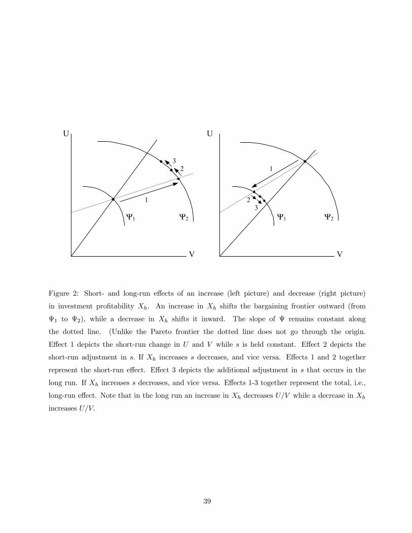
U U 3 2 1 1 2

3 Ψ1 Ψ2 Ψ1 Ψ2

V V

Figure 2: Short- and long-run effects of an increase (left picture) and decrease (right picture)

in investment profitability Xh. An increase in Xh shifts the bargaining frontier outward (from

Ψ1 to Ψ2), while a decrease in Xh shifts it inward. The slope of Ψ remains constant along

the dotted line. (Unlike the Pareto frontier the dotted line does not go through the origin.

Effect 1 depicts the short-run change in U and V while s is held constant. Effect 2 depicts the

short-run adjustment in s. If Xh increases s decreases, and vice versa. Effects 1 and 2 together

represent the short-run effect. Effect 3 depicts the additional adjustment in s that occurs in the

long run. If Xh increases s decreases, and vice versa. Effects 1-3 together represent the total, i.e.,

long-run effect. Note that in the long run an increase in Xh decreases U/V while a decrease in Xh

increases U/V.

39

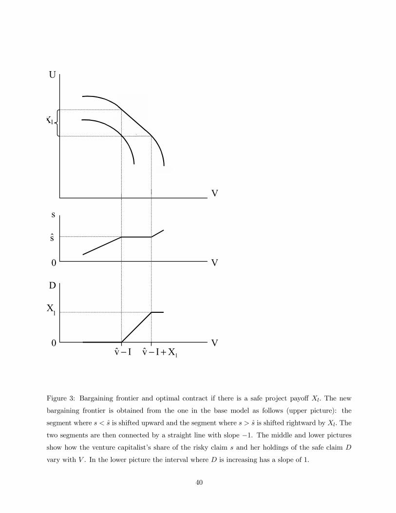
U

Xl

V s

s

0 V

D

Xl

0

Iv −

lXIv +− V

Figure 3: Bargaining frontier and optimal contract if there is a safe project payoff Xl. The new

bargaining frontier is obtained from the one in the base model as follows (upper picture): the

segment where s < s is shifted upward and the segment where s > s is shifted rightward by Xl. The

two segments are then connected by a straight line with slope −1. The middle and lower picturesshow how the venture capitalist’s share of the risky claim s and her holdings of the safe claim D

vary with V . In the lower picture the interval where D is increasing has a slope of 1.

40

U Xl V s s

0 V D-w Xl 0

Iv −

lXIv +− V

Figure 4: Bargaining frontier and optimal contract if there is a safe project payoff Xl and wage

payments are potentially unlimited. The logic is similar to Figure 3. As the safe claim and wages

are perfect substitutes only the sum D −w is uniquely determined. Since wage payments are puretransfers there now always exists a Pareto optimal allocation where the venture capitalist has a

utility of zero.

41