The Effect of Subway Access on School Choice

Luis Herskovic

herskovic@uchicago.edu

January 25, 2017

Abstract

One of the goals of school choice is to allow parents to send their children to higher-performing schools. Several studies have shown that distance to school is one of the maindeterminants of school choice, but challenges to address endogeneity issues remain. Thispaper examines school choice in a context where vouchers have been implemented on alarge scale and combines that analysis with a natural experiment to address the endogene-ity concern posed above. In particular, I use information from Santiago, Chile, and takeadvantage of the construction of a new subway line that crosses a large area of the citypreviously unconnected to the subway network. I provide convincing evidence to show thatthe introduction of the subway line was arguably exogenous for families living close to thenew subway stations. The high clustering of schools in certain areas of the city makes dis-tance especially relevant for students who live in neighborhoods with little connectivity totransport networks. The use of rich administrative data allows me to calculate the distancefrom students’ homes to each school in the city with high accuracy. Using an independentcross-sample difference-in-difference estimation, I find that (i) students near the new subwaystations travel significantly farther to school than students who live in nearby areas withno subway stations, and (ii) that students near the subway are willing to travel farther toattend schools that perform better in standardized tests. This set of results is particularlyinformative for the ongoing school-choice debate, reconciling the advocates’ and skeptics’views in the sense that school choice may lead to higher-performing schools once accessrestrictions are eased.

I Introduction

School choice was introduced to the Chilean school system in 1981 with the intention of gen-

erating competition among schools that would lead to an increase in the overall quality of the

system. The idea behind this reform was that, if schools competed to attract students and par-

ents valued quality, schools would improve their performance (Friedman, 1962, 1997). However,

this policy does not seem to have produced the desired results (McEwan et al., 2008).

In many areas of the city with low-performing schools, students do not leave their districts

to attend better schools. As I show in this paper, in Santiago during the year 2003, more

than 85% of students living in the south side of the city attended schools in their own district

despite the fact that schools in that area were performing worse than schools in the rest of the

city. If students are not actively choosing better schools, the system does not improve as a

result of implementing a school-choice policy. Did school choice fail to generate a system-wide

improvement because parents don’t value school quality as much as expected?

Some authors, such as Elacqua and Fabrega (2004) have argued that parents are uninformed

consumers when it comes to school choice, claiming that they “use few sources of information

and have weak educational networks, consider few schools in their choice set, choose based on

practical reasons, and handle very little precise information about the schools they choose.”

Others, like Gallego and Hernando (2008) have disputed this claim, showing that quality seems

to be one of the main factors affecting parents’ choice of a school. Their results show that,

in Santiago, “differences in quality seem to be the most important factor driving the decision

to attend school in the home or other municipalities.” These opposing views have persisted

throughout much of the debate on the merits of the Chilean school-choice system.

It is possible, however, to reconcile the idea that parents do care about quality with the

fact that in many cases they choose schools that are closer to their home instead of better-

performing schools that are farther away. In this paper, I claim that one of the factors that

determines school choice is access to transportation. Families sometimes will choose lower-

performing schools not because they don’t care but because the commute to better-performing

schools is too long.

To test this idea, I take advantage of a natural experiment generated by the opening of a

new subway line at the end of the year 2005 in Santiago, Chile. The inauguration of this subway

1

line and the use of GIS tools, alongside a rich administrative dataset with detailed geographic

information, allows me to estimate the effect of improved access to transportation infrastructure

on school choice while addressing endogeneity issues.

This estimation strategy is based on the fact that the subway gave easier access to more

and better schools to families living near the new subway stations but not to families in the

same neighborhoods living farther away from the stations. Because of this, if families living

near the new stations valued school quality, we would expect them to send their children to

better-performing schools than families living farther away from the new subway line.

It can be argued that having access to the subway reduced transportation costs for students.

Even if the cost of a subway ticket is the same as a bus ticket in Santiago (roughly $1), there

was a considerable reduction in travel time when using the subway. This allowed students to

potentially travel longer distances in the same time as their previous commute once the subway

was inaugurated.

Using an independent cross-sample difference-in-difference estimation, I find that students

who gained access to the subway with the construction of the new line traveled distances that

are about 20% greater to get to school than students who lived farther away from the subway,

and that the students with close access were willing to travel longer distances to attend schools

that scored higher in standardized tests than students with worse access to the subway network.

Thus, when travel times are reduced by better transport connectivity, families actually choose

better-performing schools for their children, even if these schools are farther away.

This is in line with the evidence presented by Hastings et al. (2007), who show that parents

for whom academic achievement is important are willing to leave their neighborhood to have

access to better schools. Families face a trade-off between choosing a school with a shorter

commute and choosing a school of higher quality. As the results of this paper show, when the

restriction imposed by long commute times is eased, parents choose better-performing schools

for their children.

This paper contributes to the literature on school choice, establishing that ease of access to

transportation plays a prominent role in the schooling decisions made by families. Providing

better access to schools helps parents make quality-oriented decisions. This shows that parents

do care about school quality and that school choice combined with policies that improve access

2

may result in system-wide improvements.

As school choice expands in the United States and other countries, it is especially relevant

to understand which factors may have a direct effect on the potential success of this policy.

Implementing a policy based on school choice with the goal of helping low-income students

will have little or no effect if these same students do not have access to high-quality public

transportation.

It is worth considering that even if all families care about getting higher-quality education,

some families face greater restrictions in terms of the time it takes for their children to travel to

school. Students living in districts without good schools and without good transport connec-

tivity may end up being forced to choose worse schools than what their preferences for quality

would indicate. This limits the impact that school choice may have as a policy on individual

students and on the whole system as schools do not face as much competition as they could be

facing.

The paper is structured as follows. Section II provides additional background on school

choice, on the spatial distribution of schools, on the number of students who choose schools in

other areas of the city, and on the subway network in Santiago, Chile. Section III describes the

unique dataset and distance calculations used in this paper. Section IV introduces the strategy

used to estimate the independent cross-sample difference-in-difference specification. Section V

presents the results of the estimation of the effect of subway access on school choice. Section

VI presents robustness checks. Section VII concludes the paper.

II Background

The following subsections briefly discuss school choice within the Chilean school system, the

spatial distribution of schools in Santiago, and descriptive statistics for these schools. They

also present an overview of the subway network and its expansion.

II.A School Choice in Chile

Starting in 1981, Chile began to implement an educational reform based on giving parents

freedom in the choice of their children’s school with the goal of improving the quality of the

school system. This is clearly summarized by Hsieh and Urquiola (2002): “The notion that

3

free choice is welfare enhancing is one of the foundations of modern, market-oriented societies.

This view is prominent in the school-choice debate, where there is a widespread perception that

public schools are inefficient local monopolies, and that the quality of education would improve

dramatically if only parents were allowed to freely choose between schools.”

An interesting aspect—one that makes Chile a natural ground to study the effects of school

choice—is that this reform consisted of a widespread voucher program that has lasted for more

than 30 years, providing a unique case in the context of voucher programs. For a more detailed

treatment of how the school system reacted to this reform over time, see Hsieh and Urquiola

(2002) and McEwan and Carnoy (2000).

As part of the reform, the Chilean school system was organized around three types of

schools: private, public, and voucher schools. Students could attend schools in any part of the

city and received vouchers for public or voucher schools, with some voucher schools requiring

an additional copayment by parents. That system still stands today but is the focus of major

reforms.

Despite the long-running nature of this reform, the evidence on whether school-performance

improved in Chile after implementing school choice in the 1980s is mixed. International evalua-

tions do not show clear improvements. As Hsieh and Urquiola (2002) point out when examining

international test data from TIMMS: “Using these exams we can assess whether years of unre-

stricted school choice have improved Chile’s performance relative to the other countries... The

evidence presented shows that its relative ranking, if anything, has worsened.”

One of the main arguments of the proponents of school choice—based on Milton Friedman’s

proposals—is that competition should induce schools to either improve their performance or

disappear from the educational market, being replaced by better schools (Friedman, 1997).

Again, in Chile it is not evident that this has happened. Corvalan and Roman (2012) show

that over 1,000 schools in Chile that have persistently underperformed in standardized tests

have remained in the school system over time even when most of them are located in competitive

environments, that is, with better-performing schools in nearby areas.

A frequent explanation to this apparent shortcoming of school choice has been that parents

don’t assign enough importance to quality when they choose a school (Elacqua and Fabrega,

2004). If parents care more about other factors, such as distance, religion or infrastructure,

4

schools won’t have incentives to improve their academic performance to attract more students.

This is supported by survey evidence gathered by Elacqua et al. (2006), who conducted face-

to-face interviews with parents in Santiago to study the determinants of school choice. They

conclude that “despite the fact that parents in Santiago say they are seeking strong academic

programs in their children’s schools, they actually shop for schools that are widely different on

academic quality but similar on socioeconomic dimensions. In short, as parents choose schools

in Chile, class—not the classroom—may matter more.”

This follows the claims made by Hsieh and Urquiola (2002) who suggest that when families

try to choose the best schools for their children, they may actually be trying to choose the best

peer group. Additionally, they suggest that schools may respond to the incentives generated

by school-choice policies but possibly do so by trying to attract better students in addition to

improving their quality.

Other authors have argued that school quality does play a preeminent role in school choice.

For example, Gallego and Hernando (2009) model school choice using information for 70,000

fourth-graders in Chile. They conclude that households consider several attributes when choos-

ing schools but that the two most important ones are test scores and distance from home to

school.

Regarding school choice and the relationship between distance and school quality, Hastings

et al. (2007) have argued that there is considerable heterogeneity in preferences for schools,

pointing out that “while many parents are very inelastic with respect to school test scores,

there is a significant density of parents who highly value school scores and have low preferences

for their neighborhood school. These parents are willing to consider schools outside of their

neighborhood, and they place a high weight on average test scores when picking a school.”

Chumacero et al. (2008) looked into the importance of distance from home to school when

parents choose a school in Santiago. Even though they did not have the exact location of

students’ households, they estimated a probit model and found that there was a trade-off

between distance and quality. They also found that parents were more likely to choose a school

closer to their home if their child was a girl.

5

II.B Spatial Distribution of Schools in Santiago

The previous section highlights the relevance that the distance between homes and schools may

have when analyzing school choice. Families living in certain areas of the city may not have a

realistic possibility of sending their children to better-performing schools, even if they want to.

This is even more relevant in a city like Santiago in which schools are highly clustered by type

and performance on standardized tests.

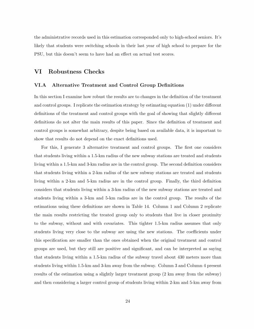
To illustrate this, I generate maps using inverse-distance-weighted interpolation (IDW) that

reflect that, despite there being over 2,000 schools in the city, they are not spatially distributed

in a way that makes them easily accessible to all families. Private schools, which outperform

voucher and public schools in standardized tests, are in many cases more than 10 km away for

a large number of students. The same applies to families that may want to send their children

to high-performing schools. Using standardized math test scores as a measure of quality, it also

becomes clear that high-performing schools are spatially autocorrelated. Figure 5 shows the

distribution of university entrance exam scores for each type of school in 2007.

The maps in Figure 1 and Figure 2 show, respectively, that private and high-performing

schools are highly clustered in the northeast area of the city. In Figure 1, greener areas reflect

a higher proportion and clustering of private schools, yellow areas indicate a larger number

of public schools, and red areas indicate a higher concentration of voucher schools. Figure 2

displays schools according to their performance in the math section of the SIMCE test on a color-

scale that goes from green for the highest-performing schools, to red for the lowest-performing

schools.

These figures present a visual representation of the challenge faced by students from other

parts of the city who want to attend a high-performing school. Without good public trans-

portation, the costs of attending a better school in terms of travel time may be too high for

many students. The construction of a faster mode of transport, such as the subway, plays a

large role in diminishing the importance of these large distances and expands the possible set

of schools from which parents can choose. The subway line that was inaugurated in late 2005

reduced travel times from southern areas of the city to the north by more than 50% for subway

users compared to bus users.1

1As an example, traveling from the southern end of the subway line to its northernmost station on a Mon-

6

The potential benefits of school choice rest on the assumption that students will actually

choose schools in other areas of the city if there are no good schools close to their homes.

This does not seem to be the case in several municipalities in Santiago. To show this, I analyze

administrative records for the years 2003, 2005, and 2007 provided by the Ministry of Education

for all students in the city. These records do not have students’ exact addresses, but they do

register the municipality the students reside in. Unlike the data I use to estimate the model,

this dataset contains information about students from all grades. I use this information to show

that a large proportion of students does not leave their own municipalities to attend schools in

other parts of the city.

Table 1 shows the percentage of students who went to schools inside their own municipal-

ities for the years 2003, 2005, and 2007 in Santiago. As can be seen, the percentage remains

relatively stable at around 70%. That is, almost three out of four students did not leave their

municipalities to attend school. This overall percentage however, hides large variations across

municipalities.

This becomes clear when examining the spatial distribution of students who do not leave

their municipalities for school, as the percentages vary widely by city area. I generate a map

to show the percentage of students attending school in the same municipality as they reside in,

which is shown in Figure 3.

This map shows percentages for students attending schools in the same municipality as they

live in, aggregated for each municipality. Municipalities in which most students travel to schools

in other municipalities are displayed in green. Red areas show places in which more than 85%

of students are living and attending schools inside the same municipality.

The map shown in Figure 3 reveals what might be an unexpected scenario for a city that

in the year 2003 had been under a school-choice system for more than 20 years. In several

municipalities, despite having mostly underperforming schools, high percentages of students

did not leave their own municipality to find better-performing schools. In many cases, more

than 90% of students living in a municipality were also studying there.

Without establishing any causality, this figure gives a first impression of the importance

of access to transportation. Municipalities which had subway stations seem to also have been

day morning at 8AM, takes about 1 hour and 40 minutes by bus, but only 35 minutes by subway, according toGoogle transit data.

7

generally the ones that had the highest percentages of students traveling to take advantage of

the possibility of attending schools in other parts of the city.

II.C Descriptive statistics of schools in Santiago

Finally, to understand the context of school choice in Chile, it is relevant to observe the evolution

of schools by type in Santiago over time, and the way students have distributed among these

types of schools during the 2003-2007 period.

Table 2 shows the number of schools in Santiago per year by type of school. As this table

shows, the number of private schools declines slightly during this period, while the number of

public schools remains relatively stable. The number of voucher schools increases moderately

but consistently every year, reflecting a trend that has been a permanent fixture since they were

introduced. Overall, the number of total schools increased from 2,116 in 2003 to 2,332 in 2007.

Table 3 shows the number of high-school seniors by type of school each year. Overall

enrollment gradually increased over time during the 2003-2007 period. Consistent with the

previous table, the number of seniors in voucher schools increased more than the number of

seniors in other types of schools.

As these tables show, the number of schools in the city increase by about 10% between 2003

and 2007. This is explained exclusively by the creation of new voucher schools. This increase in

the number of schools would represent an expansion of the possible choice set of parents when

choosing schools for their children, only if they have the means of actually attending those

schools. As I will show, this seems to be in part determined by access to public transportation.

II.D Subway network

Understanding the importance of access to transportation requires a brief overview of the sub-

way network. Santiago is a city with a population of more than 6 million people, in which in

the year 2013 more than 60% of trips in public transport were subway trips (Metro de Santi-

ago, 2013). The subway network construction began in 1969, and the first line (Line 1) was

inaugurated in 1975. In 1978 the second line (Line 2) opened, followed by the third line (Line

5) in 1997.

Between November 2005 and March 2006, the fourth line (Line 4) of the subway system

8

started operating. Line 4 is the longest line in the network, covering 24 km with 23 stations,

and extending across 7 large municipalities. It transports around 500,000 people every day and

it’s connected to the other 3 lines in the subway network (Metro de Santiago, 2013; De Grange,

2010).

As I show in Table 4, the yearly ridership of the subway network in Santiago increased

during the 2003-2007 period. Line 4 was inaugurated at the end of 2005, but some stations

were not fully functional during part of 2006. This is reflected in the lower number of passengers

during those years. By 2007 the line reached its maximum operating capacity with almost 115

million passengers per year.

Before the expansion in 2005-2006, a vast area containing some of the most populated

neighborhoods in the city was poorly connected to the transportation network, which consisted

of Line 1, Line 2 and Line 5. Figure 4 shows what the subway networked looked like after the

inauguration of the new subway line (Line 4) at the end of the year 2005. The network in the

year 2016 transports more than 2 million passengers per day.

As I illustrate in Figure 4, Line 4 stretches towards the south of Santiago and is connected

to the rest of the subway network. This is relevant because the new subway line connected a

large area of the city that previously suffered from poor connectivity, greatly reducing travel

times. Using the Google Distance Matrix, I performed several travel simulations of bus and

subway trips between this southern area of the city and the northern end of Line 4, and found

that travel time on average was reduced by about 50% when traveling by subway instead of by

bus.

III Data, variables, geocoding and distance calculations

To study the impact of the subway on school choice I use rich yearly administrative data

which contains information on students’ home addresses, school addresses and subway station

addresses. I geocode every one of these addresses to find the coordinates that identify their

exact location. Once students’ homes have been geocoded, I identify which students live near

the area of influence of the subway, and I also identify the students that live farther away. Then

I calculate the distance between home and school for every student in the dataset. The details

of this are explained in the sub-sections that follow.

9

III.A Datasets

The main dataset I use for this study is generated from yearly Prueba de Seleccion Universitaria

(PSU) registration forms from the years 2003 to 2007. During their high school senior year,

Chilean students interested in attending higher education submit a registration form to take

this test, which can be considered an SAT equivalent with a mathematics and language section,

and other optional additional sections. The PSU test has a minimum score of 150 points, a

maximum of 850, a mean of 500 points and a standard deviation of 110. I consider only students

that are taking the test for the first time, and leave out students that are are registering to

re-take the test since they are not high school seniors.

This dataset contains information on students’ age, gender, test scores, GPA, the school

they attended on their senior year, number of family members that are working, and their

home address when registering for the test. Data is only available for high-school seniors each

year, so I compare each year’s cohort with the seniors from the other years in the 2003-2007

period.

It is important to note that students that do not register to take the PSU, cannot be included

in this analysis. About 80% of high school seniors register for the PSU each year, with students

from lower socio-economic backgrounds being the ones that usually don’t register for the test

(Consejo de Rectores de las Universidades Chilenas, 2015), which restricts the interpretation of

the results of this study to students that registered for the test.

The second dataset I use is generated from SIMCE2 test score results. This test, established

in 1988, is applied yearly to all 4th graders in Chile, and on alternating years to 8th and 10th

graders. It measures achievement in mathematics and verbal skills. Additional test subjects,

such as an English language proficiency test, have been added over time. Possible scores range

from 200 to 350 points, with a mean of 250 points and a standard deviation of 50.

The SIMCE data I use is aggregated by schools. In this study I look at average SIMCE

math scores by school, and also take advantage of this dataset, using it as a census of all schools

in the city, including the address of each school and the year it was established. It is relevant

to point out that SIMCE results are widely reported on and the Ministry of Education devotes

large amounts of resources to disseminate the results for each school in various ways.

2SIMCE is the Spanish acronym for Quality of Education Measuring System

10

Every year during the 2003-2007 period considered in this paper, between 50,000 and 60,000

high school seniors register to take the PSU for the first time. I am able to accurately geocode

more than 90% of students’ home addresses each year. I consider results as accurate if the

coordinates obtained are either a precise street address or a named route. Addresses geocoded

as sublocalities, neighborhoods or other administrative area levels are left out of the final sample.

III.B Variable definitions

I consider three alternative outcome variables in this paper: home-school distance in meters, the

logarithm of home-school distance, and rank-distance of schools. The first of these outcomes is

the distance between home and school. Since the datasets contain home and school addresses,

I geocode them to obtain their exact latitude and longitude with the objective of being able to

calculate distances. It’s important to note that this is not a measure of travel-time, which would

require an assumption about the transport mode used by students, such as car, subway, bus,

or walking. Calculating distances as I do in this paper approximates a realistic travel pattern

for urban areas regardless of transportation mode. I explain this process in more detail in the

next subsections.

The second outcome is the logarithm of the distance between home and school. This outcome

allows for a more intuitive interpretation, in which the coefficient of interest indicates the

percentage change in the distance traveled to school once the subway line is inaugurated.

The last outcome is the rank-distance of schools, which produces results which require an

alternative interpretation. For this, I rank schools for each student according to their distance

from that student’s home. For example, the school closest to a student’s home is ranked number

one, the second school in distance to that house is ranked number two, and so on. In this way,

a rank of 100 means that a student had 99 schools closer to her home than the school she chose

to attend. This rank shows how many schools a student skips over in terms of distance before

choosing the school she finally attends. The relationship between rank-distance and home-school

distance in the year 2003 and 2007 is shown in Figure 9 and Figure 10, respectively.

The treatment variable is defined as students that live near a new subway station. That is,

students living in a 2.5-km radius of a new subway station are considered as treated. Students

living between 2.5 km and 4 km from a subway station are part of the control group.

11

The choice of these precise distances is somewhat arbitrary, although based on other studies

of subway use. For example, a study of dutch rail stations shows that usage of stations largely

declines as the distance between residence and station increases, and the largest declines seem

to happen at around 3 kilometers from the station (Keijer and Rietveld, 2011). As shown in

Section VI, slightly different distance definitions does not alter the results.

I also consider several control variables in the estimation. Among them, I look at the number

of schools in a 1-km and 5-km radius from the student’s home (I also test several other distances,

which does not alter the results). This allows me to control for the fact that students living

near the subway also live closer to a larger number of schools, since understandably schools are

more often located in larger avenues which coincide with the places the subway line is built

through.

Other variables I consider as controls are the number of a student’s family members that

are currently working and the student’s gender. Finally, I also consider the type of school the

student attends, which can take 3 possible values: public, voucher, or private.

III.C Geocoding

I geocoded approximately 200,000 student home addresses for this paper. For this purpose, I

developed a custom script that first corrected errors in the addresses and then, over several

months, used a combination of geocoding services provided by Google and ESRI to find the

coordinates of homes and schools. This process made it possible to achieve a high level of

accuracy (defined as either “rooftop” addresses, or routes), reflected by the fact that for each

year of data, I was able to geocode about 90% of addresses accurately. This differs from other

papers using Chilean data that have used distances measured from the center of municipalities,

which may be several kilometers away from actual home addresses.

III.D Home-school distance calculations

The first outcome of interest in the estimation is the distance between home and school. There

are several possible ways to calculate these distances. For simplicity, a considerable number of

previous research papers have used a “straight-line” distance calculation to measure the distance

between 2 points. But since in this paper I am measuring distances within urban areas, it is

12

much more accurate to use what is commonly referred to as “block” or “Manhattan block”

distance (Boscoe, 2013).

The difference between these 2 types of measurements is non-trivial, since even when looking

at a distance as short as a few city blocks, using a straight-line calculation will yield a distance

considerably shorter than the more realistic block calculation.

As a simple example of this, note that if a student travels only two standard city blocks

of 100 meters each to get to school, which include turning a corner, the straight-line distance

calculation underestimates the distance traveled by 30% compared to the block-distance calcu-

lation.

The formula used to calculate block distance follows Gimpel and Schuknecht (2003):

di = |xi − xj|+ |yi − yj|,

where xi is the longitude of home i, and yj is the latitude of school j. As stated, this formula

assumes that students don’t travel in a straight line between home and school, which is a more

realistic representation of travel patterns within cities.

Table 5 shows the average distance traveled by students to get to their school by year. As

can be seen, the average distance is about 5.5 km and it decreases slightly over time. One

possible explanation for this is the increasing overall number of schools in the city as shown

previously in Table 2.

IV Estimation Strategy

I use an independent cross-sample difference-in-difference specification to estimate the effect

of subway access on school choice. In this approach, variation is determined by the distance

between houses and the new subway stations, which in the short term should be arguably

exogenous. The validity of this method would be threatened if families living near the subway

would have changed the average distance they travel to school relative to families living farther

away regardless of the construction of the subway line, or if certain types of families were more

likely to locate closer to the subway than others. This is partly addressed by considering a

period close to the opening of the subway line, comparing characteristics between groups before

13

and after the subway opened, and examining the trends followed by each group.

Regarding this same issue, it is important to point out that although Line 4 was publicly

announced during 2001, the initial announcement only revealed the general placement of the

line with no information on specific stations. One way to address the possibility that families

who cared more about education may have moved to homes near the subway is to look at

changes in housing prices at the time the subway line was announced. Agostini and Palmucci

(2005) do this and find that housing prices near the new subway line reacted in a very limited

magnitude to the announcement, increasing around 3% with respect to locations farther away

from the line. This would seem to indicate that a massive displacement of people living near

the subway did not take place.

Additionally, in this paper I consider a period of time that begins shortly before the inau-

guration of the subway line and ends after it has been operating for only one year. This may

also reduce concerns about the area surrounding the stations changing its social composition or

infrastructure because of the new subway. Finally, in Section VI, I present results considering

only the years before the subway line opened. This also provides evidence that supports the

idea that students living near the area where the subway stations were constructed, were not

traveling longer distances to school before the subway was inaugurated.

A different threat to the identification strategy proposed in this paper would be the possi-

bility that schools are selecting students instead of families selecting schools. That is, if schools

are the ones controlling which students are admitted, it would be possible for them to select

students based on characteristics that would capture differences besides access to the subway.

This, however, does not seem to be the case in Chile. The evidence points in the opposite

direction. That is, families are the one making these decisions, not schools. Gallego and

Hernando (2008) show that sorting in the Chilean school system comes from the demand side

and not from the supply side. They point to evidence from a 2006 survey, which found that

93% of parents actually said that their children were attending the school they had wanted to

choose as their first option. Supporting this, parents applied on average to only 1.1 schools.

14

IV.A Treatment and Control Groups

For the analysis that follows, I consider that people who live close to a subway station are more

likely to use the subway than people who live farther away. With this in mind, I define the

treatment and control groups as follows: the treatment group is composed of high-school seniors

living within a 2.5-km radius of a new subway station. The control group comprises high-school

seniors living between 2.5 km and 4 km from a new subway station. Figure 6 presents a map I

generated by using a fishnet that captures students in each group to show this more clearly.

Table 6 shows a comparison of several relevant variables between control and treatment

groups before the subway line opened in the year 2003. In Table 7, I show this comparison for

the year 2007, that is, after the subway line opened.

The first of the variables shows the average distance traveled by students to their chosen

school. Students in the control group in the year 2003 traveled longer distances on average to

get to school than students in the treatment group: 6.2 km vs. 5.5 km, respectively. This could

be explained by the fact that the control group had fewer schools near their homes, as shown

by the average number of schools closer than 1 km and 5 km. Students in the control group

had then on average 117 schools within a 5-km radius of their homes, while students in the

treatment group had 143. It is important to point out that while there are differences in the

values of these variables between groups, the differences remain similar over time except for the

distance traveled to school, which is the outcome of interest.

These variables help address the possibility that schools may have reacted to the new subway

line by positioning themselves near stations to attract more students. This could affect the

estimation, since students in the treatment group would suddenly face an increase in the number

of schools near their homes. This does not seem to be the case, as shown in Tables 6 and 7, since

the number of schools within a 1-km radius from the students living close to subway stations

was 7 in 2003 and 2007 and the number of schools within a 5-km radius changed from 143 to

142.

The percentage of students who are male also is similar between groups—close to 50% for

the treatment and control groups—before and after the subway was built. Students in the

control group attended schools that scored on average 275 points on the SIMCE math test in

2003 and 271 points in 2007. Meanwhile, schools attended by students in the treatment group

15

scored 277 points in 2003 and 272 in 2007. Finally, the average number of family members

who were working was 1.5 for both groups in 2003 and 1.3 for both groups in 2007. As can be

seen in Tables 6 and 7, all of these variables have similar values and their differences remain

practically constant over time.

IV.B Pre-treatment Trends

Defining the groups as explained in the previous section makes it likely that the treatment and

the control groups will experience similar changes in their characteristics on average, although

students in the treatment group will be more likely to use the subway as their means of trans-

portation. These definitions are used to estimate a difference-in-difference specification, which

assumes that both groups followed similar trends before the treatment. Visually this can be

seen in Figure 7, which shows trends in covariates for each group before and after the inaugu-

ration of the subway line. There doesn’t seem to be an important change in the characteristics

of people living near the subway once the stations open. This helps address the possibility that

once the subway opened, people with a specific set of characteristics may have immediately

moved to areas surrounding the subway.

The panels in Figure 7 show several trends followed by the treatment and control groups.

Panel (a) shows the percentage of students in each group that attends public schools. As can

be seen, both groups follow relatively parallel trends over time, with about 25% of students

attending a public school. As has been commonly observed in Chile, this percentage gradually

declines over time. The relationship between the trends followed by both groups remains con-

stant even after the subway line is operating in 2006 and 2007.

Panel (b) shows the senior-year grade average for both groups. This panel shows that there

were no differences in the achievement of students in the treatment and control groups once the

subway started operating and that they followed very similar trends between 2003 and 2007.

Panel (c) shows the average distance between the closest school and each student’s home. It is

important to point out that this is not the distance to the actual school the student attended

but the distance to the school closest to their home. This figure reveals that students in the

treatment group, on average, had a school closer to their home than students in the control

group but also that the groups followed parallel trends over time. This did not seem to be

16

affected by the opening of the subway line, which is consistent with the idea that schools did

not immediately react to the construction of the subway line by changing their locations.

Finally, panel (d) shows the number of schools located within a 1-km radius of each student’s

home. As is the case with the other variables, even if there were more schools near students in

the treatment group than in the control group (7 and 4, respectively), which is consistent with

the results from panel (c), the groups still followed parallel trends between 2003 and 2007.

As can be seen from these tables and figures, the treatment and control groups were similar

before and after the subway was built and they followed similar trends over time. There did

not appear to be a significant event that affected one group and not the other besides the

inauguration of the new subway line.

IV.C Effect of Subway Access on Distance to School

I first estimate the effect of subway access on the distance between home and school to see

if families that got subway access sent their children to schools that were farther away than

families that did not get a station nearby. After this, I include an interaction to estimate the

quality of the chosen school to see if parents who lived near the subway were in fact choosing

better schools.

I consider that high-school seniors who lived within a 4-km radius of a subway station of the

new line in the year 2003, before it started operating, are part of the “before” group. In turn,

students who were high-school seniors in the year 2007 and who lived within a 4-km radius of

a subway station of the new line are part of the “after” group.

The group that lived near the subway line (within a 2.5-km radius) after the subway line

opened were the students most likely to be using the subway, so they will be considered as being

in the treatment group, while the rest of high-school seniors, who lived between 2.5 km and 4

km away from the subway, will be considered as being in the control group.

The key identifying assumption of the difference-in-difference estimation is that both groups

would have followed similar trends if the subway line had not been built. Even if it’s not possible

to test this assumption directly, by looking at graphs of the trends of each outcome variable

it’s possible to see whether both groups followed parallel trends until the subway line was

inaugurated.

17

I show the parallel trends first for the distance between home and school in Figure 8. As the

lines in the chart show, individuals in the treatment and control groups followed similar trends

in the years before the subway opened. Students in the treatment group traveled on average

about 5,500 meters to go to school, while students in the control group traveled almost 1,000

meters more. Both trends are parallel until the subway opens, which caused students living

near the subway to start attending schools that were farther away from their homes.

The same pattern is present when looking at the alternative outcome, rank-distance to

school, as presented in Figure 11. The figure shows that, for example, that students in the

treatment group in 2003 on average, had almost 210 schools closer to their homes than the

school they were actually attending. Each year, students attended schools closer to their homes

in terms of rank-distance, but once the subway opened, students living near the subway started

skipping over more schools than students in the control group.

The key equation that I estimate is the following:

Distanceit = β0 + β1Subwayi + β2Postt + γ(Postt ∗ Subwayi) +Xit + ǫit (1)

in which the outcome variable, Distance, is the block distance in meters between a student’s

home and their school, for student i in year t. I also estimate equation (1) using the logarithm

of distance between home and school and the rank-distance of schools as alternative outcome

variables. Subway is a binary variable that is set to one for students that live in houses that

are within a 2.5-km radius of a new subway station. Post is a binary variable that is set to one

if a student is a member of a cohort that graduated from high school after the new subway line

was built.

The parameter γ, which corresponds to the difference-in-difference estimator, captures the

effect of increased subway access on the distance between the school a student was attending

and their home. It is important to note that this parameter captures the intention to treat,

since the available data does not contain information that could be used to identify whether

students were using the subway. Nonetheless, it seems reasonable to assume that students living

closer to the subway were more likely to use it than students living farther away.3

3Information available from a large-scale transportation survey conducted in 2012 in Santiago shows thatin the municipalities that surround the subway line studied in this paper, only about 35% of adults have adriver’s license, and about half of the households don’t own a car. About one third of all subway passengers

18

If students who lived near the subway started attending schools that were farther away from

their homes after the subway opened, we should expect to observe a positive and significant

coefficient for this parameter.

X it is a vector of control variables, which includes the gender of the student, a variable

indicating if family members worked, the number of schools that were closer than 1 km to the

student’s home, the number of schools that were closer than 5 km to the student’s home, and

dummy variables for the type of school, where private schools are the omitted category. Since

the identification strategy being used does not depend on the inclusion of these covariates, it is

expected that they should not affect the results.

IV.D Effect of Subway Access on Distance to School by Test Scores

Additionally, I also estimate a model that includes the interaction between the treatment group

and a measure of school performance: standardized math test scores. The idea behind this is to

see if students living near the subway were traveling farther away to get to a better-performing

school. There is some evidence that shows that families have not generally been aware of SIMCE

results (Corvalan and Roman, 2012). It is possible, though, that awareness increased over time,

since scores are now widely reported on news coverage and the Ministry of Education at various

times has released maps and other types of reports showing easy-to-understand representations

of the test score of each school.

The key equation in this case is the following:

Distanceitj = β0 + β1Subwayi + β2Postt + β3Testj + β4(Postt ∗ Subwayi)+

β5(Postt ∗ Testj) + γ(Postt ∗ Subwayi ∗ Testj) +Xit + ǫitj

(2)

in which the outcome variable is the block distance in meters between a student’s home and

school, for student i and school j in year t. I also consider the alternative outcomes used

previously: the logarithm of the distance between home and school and the rank-distance of

schools.

The Test j variable corresponds to the SIMCE test math score of school j, which range from

200 to 350 points..

are students (OSUAH, 2012).

19

The parameter γ now captures the effect of increased subway access on the distance traveled

to school when attending a school that scores higher on standardized tests. Thus, if students

near the subway were willing to travel farther to attend better-performing schools, this coeffi-

cient should be positive and significant.

X it is a vector of control variables, which includes the gender of the student, a variable

indicating if family members worked, the number of schools that were closer than 1 km to the

student’s home, the number of schools that were closer than 5 km to the student’s home, and

dummy variables for the type of school, where private schools are the omitted category.

V Data Analysis and Results

In this section, I look at the results from the estimation of the effect of subway access on the

distance between home and school, its interaction with school performance, and results for

sub-groups of students.

V.A Results: Effect of Subway Access on Distance to Chosen School

The first set of results presented in Table 8 are from the estimation of equation (1), with and

without covariates, using three different outcomes: the home-to-school distance in meters, the

logarithm of the home-to-school distance, and the school rank-distance. Columns 1, 3 and 5

present estimations without covariates, while Columns 2, 4 and 5 include covariates.

The estimated effect of subway access on distance between the chosen school and students’

homes is positive and significant, and it is practically unchanged when adding control variables,

as was expected. The coefficients in Columns 1 and 2 show that having access to the subway

results in attending schools about 600 meters farther away on average than students who did

not live near the subway, which represents an almost 10% increase over the average distance

traveled by all high-school seniors in the city, not just those in the control group.

Columns 3 and 4 in Table 8 also reveal interesting results. The coefficient of 0.2, using

log distance as the outcome variable, can be interpreted as showing that having access to the

subway allowed students to choose schools that were 20% farther away than students in the same

neighborhood who did not get direct access to the subway. This result is important because

it shows that students are willing to travel farther away to school if they have access to faster

20

transportation. The new subway line reduces travel time, and this allows students living close

to the stations to travel larger distances than they could before it opened.

Finally, Columns 5 and 6 in Table 8 present results using the alternative outcome of rank-

distance to school. This allows for a complementary yet alternative interpretation. The positive

and significant coefficient of 24.2 shows that students in the group treated by the subway skipped

an additional 24 schools when choosing a school to attend, compared to students in the control

group. That is, they went 24 schools farther away than they would have if they had not received

access to the subway.

The full results, shown in Table 9, also reveal interesting results. Male students traveled

almost 7% farther to school than females. This is in line with findings presented by Chumacero

et al. (2008) who propose that parents are more willing to let their sons travel longer distances

to school than their daughters.

The presence of more schools near a student’s home (closer than 1 km and closer than 5 km)

is associated with a decrease in the distance students travel to school, as would be expected.

Having an additional school within a 1-km radius of home is associated with a reduction in the

distance traveled to school of about 130 meters. The presence of an additional school within a

5-km radius has a much smaller but still negative effect on distance traveled to school.

Restricting the sample by using different definitions of the treatment and control groups does

not alter the main results. Since there is no data on which students were using the subway, it

is relevant to note that defining the treatment group as a wider or narrower area around the

new station produces similar results in terms of the direction and magnitude of the effect. This

is shown in more detail in Section VI.

V.B Results: Effect of Subway Access on Test Scores of Chosen School

The results presented in the previous section show that subway access had a relevant effect on

the home-school distance traveled by students living near the new subway, but these results do

not address the question about what is the performance in tests of chosen schools. Table 10

examines the results of the estimation of equation (2), which introduces the interaction with

school test scores. These results are relevant because once it is established that families living

near the subway choose schools that are farther away, it is important to know if the schools they

21

are choosing are better-performing than the ones chosen by families without subway access.

The coefficients in Columns 1 and 2 in Table 10 are positive and significant and do not

change substantially when control variables are included in the estimation. These coefficients

were obtained using distance between home and school as the outcome variable, and they

correspond to the interaction between the treated group in the period after the subway was

inaugurated and school test scores. The coefficients can be interpreted as showing that students

living near the subway traveled 12 additional meters to attend a school that scored one point

higher on a standardized math test in which scores ranged from 200 to 350 points. This is

consistent with an estimation done by Chumacero et al. (2008) who also found that students

were willing to travel an extra 12 meters for an extra point in this test.

This result is particularly important because it reflects the value assigned by parents and

students to school performance. Families were willing to send their children farther away if they

were attending better-performing schools, indicating that travel restrictions play a relevant role

in school-choice policies. Parents seem to value school performance, but it’s possible that

students face too many difficulties when trying to access better-performing schools and end up

attending schools closer to their homes that are not as high-performing as the ones they would

like to attend.

These results are similar to those derived using the log of the distance between home and

school, which are presented in Columns 3 and 4. The latter results show that students that had

access to the subway would travel 0.2% farther to attend a school that scored one point higher

on the SIMCE test. The estimations with and without covariates produce similar coefficients,

which are positive and significant.

Columns 5 and 6 show results using rank-distance to schools as the outcome variable. Again,

both coefficients are positive but only the coefficient of the estimation that includes control

variables is significant. This coefficient of 4.4 reflects that a student would skip over four

schools closer to her home to attend a school that performed one point higher on the test.

In summary, these results give clear indications that once transportation restrictions are

eased, students are willing to choose higher-performing schools even if these are farther away.

On the aggregate level, if transportation was improved for a larger number of students, we

could expect an increase in competition between schools to attract students that are now able

22

to reach a wider set of schools. This, in turn, could lead to overall increases in the quality of

the school-system, as school-choice policies originally intended.

V.C Results: Effect of Subway Access by Subgroups

Finally, I examine results from the estimation by subgroups. I separate students first by the

type of school they attended and then by how they performed on the PSU test.

First, I show that having access to the subway did not affect the type of school that a student

attended, be it public, voucher, or private. For this, I estimate a variation of equation (1) in

which the outcome is the type of school. I do this one time for each possible type of school.

This way, it’s possible to estimate the impact of subway access on the type of school chosen by

students. As can be seen in Table 11, Columns 1, 2 and 3 have coefficients that are close to 0

and not significant. This can be interpreted as showing that subway access did not affect the

type of school a student chose. Considering this result along with the previously established

results, it’s possible to state that students who got access to the subway chose schools that

performed better and that were farther away, but they did not choose a specific type of school.

Along with this, to see if results vary according to the type of school students were attending,

I again estimate equation (1), this time separately for students according to the type of school

they attended. That is, I estimate the equation three times: once for public-school students,

once for voucher-school students, and once for private-school students. The results of this

estimation are presented in Table 12. These results show that students from private and voucher

schools traveled more than 700 meters farther when they had access to the subway. Students

from public schools that had access to the subway did not attend schools that were significantly

farther away compared to students in public schools without subway access.

The second subgroup corresponds to students divided into three quantiles by their PSU

math test scores, classified as Low, Medium, or High. The goal of this is to estimate if having

access to the subway had an effect over a student’s performance on university entrance exams.

Table 13 shows that having access to the subway did not have an effect on test scores. The

coefficients in Columns 1 and 2 are not significant and close to 0. The coefficient in Column 3 is

significant at p < 0.1 and close to 0. Even if students with subway access were attending better-

performing schools, their tests scores did not improve. One possible explanation for this is that

23

the administrative records used in this estimation corresponded only to high-school seniors. It’s

likely that students were switching schools in their last year of high school to prepare for the

PSU, but this doesn’t seem to have had an effect on actual test scores.

VI Robustness Checks

VI.A Alternative Treatment and Control Group Definitions

In this section I examine how robust the results are to changes in the definition of the treatment

and control groups. I replicate the estimation strategy by estimating equation (1) under different

definitions of the treatment and control groups with the goal of showing that slightly different

definitions do not alter the main results of this paper. Since the definition of treatment and

control groups is somewhat arbitrary, despite being based on available data, it is important to

show that results do not depend on the exact definitions used.

For this, I generate 3 alternative treatment and control groups. The first one considers

that students living within a 1.5-km radius of the new subway stations are treated and students

living within a 1.5-km and 3-km radius are in the control group. The second definition considers

that students living within a 2-km radius of the new subway stations are treated and students

living within a 2-km and 5-km radius are in the control group. Finally, the third definition

considers that students living within a 3-km radius of the new subway stations are treated and

students living within a 3-km and 5-km radius are in the control group. The results of the

estimations using these definitions are shown in Table 14. Column 1 and Column 2 replicate

the main results restricting the treated group only to students that live in closer proximity

to the subway, without and with covariates. This tighter 1.5-km radius assumes that only

students living very close to the subway are using the new stations. The coefficients under

this specification are smaller than the ones obtained when the original treatment and control

groups are used, but they still are positive and significant, and can be interpreted as saying

that students living within a 1.5-km radius of the subway travel about 430 meters more than

students living within 1.5-km and 3-km away from the subway. Column 3 and Column 4 present

results of the estimation using a slightly larger treatment group (2 km away from the subway)

and then considering a larger control group of students living within 2-km and 5-km away from

24

the new subway stations. Again, the coefficients are positive and significant and show that

changing the definitions slightly does not alter the main conclusions of this paper. Finally,

Column 5 and Column 6 present results using an even larger treatment group, which considers

students living within a 3-km radius of the subway as being treated. These results are similar

to the ones obtained using the definitions considered in the main estimation. In summary, the

results presented in this paper do not depend on the exact distance ranges used to define the

treatment and control groups.

VI.B Falsification Tests

In an attempt to provide evidence that the estimation is capturing the impact of subway access

on distance traveled to school, I estimate equation (1) using only the years before the subway

line was built. If the subway is causing students to attend schools that are farther away, we

should expect to see no significant effect before the subway line was constructed. The results

of this estimation are shown in Table 15.

Column 1 and Column 2, show the results of estimating equation (1) using only information

for the years 2003 and 2004 using distance between home and school as the outcome. As

expected, the results are not significant. That is, students living near where the subway was

going to be constructed, did not travel significantly longer distances than students living farther

away. Column 3 and Column 4 show the same results using the logarithm of home-to-school

distance as the outcome, and Column 5 and Column 6 show the results using rank-distance

between home and school. The results as before, are not significant.

As a complement to this strategy, I generate placebo subway lines and reproduce the es-

timation using these non-existent lines. For this, I generate subway lines that are the same

shape and length than Line 4. I spatially offset these subway lines by altering the latitude of

the original subway stations and maintaining their longitude constant. This results in a series

of subway lines that are parallel to Line 4, which are restricted to inhabited areas in Santiago.

A map with 3 of these placebo lines is shown in Figure 12.

Using these new geographic points, I reproduce the entire procedure by calculating the

distances between every student’s home, school and subway station. I then estimate equation

(1) using these values. Since there are no real subway stations going through the areas being

25

considered, we should expect to see no effect of being treated by the placebo subway lines.

As expected, living near these placebo subway stations has no effect on distance traveled to

school. Results of these estimations using each of the 3 placebo subway lines are presented in

Table 16, Table 17 and Table 18. In each table, the first 2 Columns present results using home-

to-school distance, without and with covariates. Column 3 and Column 4 show the same results

using the logarithm of home-to-school distance as the outcome, and Column 5 and Column 6

show the results using rank-distance between home and school. None of the coefficients are

significant.

VII Conclusion

The main results from the difference-in-difference estimation show that households that gained

access to the subway started sending their children to schools that were 20% farther away, on

average, and that the students with close access were willing to travel a longer distance to

attend better-performing schools than students who lived farther away from the subway. These

results do not change when control variables are included in the estimation.

Another way of to illustrate this using an alternative outcome is to state that, after the

subway was built, parents living near the new subway stations sent their children to schools

that were on average about 24 schools farther from their homes than parents who did not have

easy access to the subway line. That is, they skipped over 24 schools that were closer to their

homes and chose schools that performed better in standardized tests.

Parents face a restriction created by problems with access to transportation when choosing

schools. When this restriction is relaxed by the construction of a new subway line, parents with

access to the subway start choosing higher-performing schools even if these are farther away

from their homes. Thus, policies that seek to improve school quality via creating a system

that increases competition between schools must necessarily consider the relationship between

access to transport systems and school choice. This set of results is particularly informative for

the ongoing school-choice debate. It is commonly claimed that school choice has not produced

system-wide improvements in Chile because parents do not care enough about school quality

when choosing schools. I show that parents care enough to send their children to better-

performing schools even if they are farther away as long as it’s a realistic possibility in terms

26

of access. A system in which schools are highly spatially segregated will be unlikely to produce

quality improvements if students have difficulties accessing the schools they would like to attend.

Schooling systems that foster competition among schools may still result in system-wide

improvements. In this case, the construction of a subway line reveals that competition might

eventually bring higher quality into the system but that it might not have an effect on its own

as long as other challenges have not been addressed.

27

References

Agostini, C. and Palmucci, G. (2005). Capitalizacion anticipada del metro de santiago en el

precio de las viviendas. ILADES-Georgetown University Working Papers.

Alderman, H., Orazem, P. F., and Paterno, E. M. (2001). School quality, school cost and the

public/private school choices of low-income households in pakistan. The Journal of Human

Resources, 36(2):304–326.

Andre-Bechely, L. (2007). Finding space and managing distance: Public school choice in an

urban california district. Urban Studies, 44(7):1355–1376.

Asahi, K. (2014). The impact of better school accessibility on student outcomes. Spatial

Economic Research Centre Discussion Paper, 156.

Bae, C.-H. C., Jun, M.-J., and Park, H. (2003). The impact of seoul’s subway line 5 on residential

property values. Transport Policy, 10:85–94.

Baum-Snow, N. (2007). Did highways cause suburbanization? The Quarterly Journal of

Economics, pages 775–805.

Boscoe, F. (2013). Geographic Health Data: Fundamental Techniques for Analysis. CAB Inter-

national.

Card, D. (1993). Using geographic variation in college proximity to estimate the return to

schooling. NBER Working Paper Series, (4483).

Chumacero, R., Caorsi, D. G., and Paredes, R. (2008). I would walk 500 miles (if it paid).

Munich Personal RePEc Archive (MPRA).

Consejo de Rectores de las Universidades Chilenas (2015). Proceso de admision 2015.

Corvalan, J. and Roman, M. (2012). The permanence of low-performance schools in the chilean

educational quasi market. Revista Uruguaya de Ciencia Polıtica.

De Grange, L. (2010). El gran impacto del metro. EURE, 36(27):125–131.

28

Denzler, S. and Wolter, S. C. (2011). Too far to go? does distance determine study choices?

IZA Discussion Paper, (5712).

Dickerson, A. and McIntosh, S. (2010). The impact of distance to nearest education institution

on the post-compulsory education participation decision. Sheffield Economic Research Paper

Series, (2010007).

Elacqua, G. and Fabrega, R. (2004). El consumidor de la educacion: El actor olvidado de la

libre eleccion de escuelas en chile. PREAL, Universidad Adolfo Ibanez.

Elacqua, G., Schneider, M., and Buckley, J. (2006). School choice in chile: Is it class or the

classroom? Journal of Policy Analysis and Management, 25(3):577–601.

Falch, T., Lujala, P., and Strom, B. (2013). Geographical constraints and educational attach-

ment. Regional Science and Urban Economics, 43:164–176.

Frenette, M. (2004). Access to college and university: Does distance to school matter? Canadian

Public Policy / Analyse de Politiques, 30(4):427–443.

Friedman, M. (1962). Capitalism and Freedom. Chicago University Press.

Friedman, M. (1997). Public schools: Make them private. Education Economics, 5(3):341–344.

Gallego, F. and Hernando, A. (2009). School choice in chile: Looking at the demand side.

Working Paper - Pontificia Universidad Catolica de Chile, Instituto de Economıa.

Gallego, F. and Hernando, A. E. (2008). On the determinants and implications of school

choice: Semi-structural simulations for chile. Documentos de trabajo, Instituto de Economia.

Pontificia Universidad Catolica de Chile.

Gertler, P. and Glewwe, P. (1989). The willingness to pay for education in developing countries:

Evidence from rural peru. LSMS Working Paper, (54).

Gibbons, S. and Vignoles, A. (2009). Access, choice and participation in higher education.

Working Paper - Centre for the Economics of Education.

Gimpel, J. and Schuknecht, J. (2003). Political participation and the accessibility of the ballot

box. Political Geography, 22:471–488.

29

Griffith, A. L. and Rothstein, D. S. (2007). Can’t get here from there: The decision to apply to

a selective institution. Working Paper - Cornell University, School of Industrial and Labor

Relations.

Hastings, J. S., Kane, T. J., and Staiger, D. O. (2007). Parental preferences and school com-

petition: Evidence from a public school choice program. Working Paper.

Holzer, H. J., Quigley, J. M., and Raphael, S. (2003). Public transit and the spatial distribution

of minority employment: Evidence from a natural experiment. Journal of Policy Analysis

and Management, 22(3):415–441.

Hsieh, C.-T. and Urquiola, M. (2002). When schools compete how do they compete? an

assessment of chile’s nationwide school voucher program. Working Paper.

jae Lee, M. and Kang, C. (2006). Identification for difference in differences with cross-section

and panel data. Economics Letters, 92:270–276.

Keijer, M. and Rietveld, P. (2011). How do people get to the railway station? the dutch

experience. Transportation Planning and Technology, 23(3):215–235.

Kjellstrom, C. and Regner, H. (1999). The effects of geographical distance on the decision to

enroll in university education. Scandinavian Journal of Educational Research, 43(4):335–348.

McEwan, P. and Carnoy, M. (2000). The effectiveness and efficiency of private schools in chile’s

voucher system. Educational Evaluation and Policy Analysis, 22(3):213–239.

McEwan, P., Urquiola, M., and Vegas, E. (2008). School choice, stratification, and information

on school performance: Lessons from chile. Economıa.

Metro de Santiago (2013). Memoria anual metro de santiago.

OSUAH (2012). Encuesta origen destino de viajes. Technical report, Universidad Alberto

Hurtado.

Phillips, D. C. and Sandler, D. (2015). Does public transit spread crime? evidence from

temporary rail station closures. Working paper.

30

Sa, C., Florax, R. J., and Rietveld, P. (2004). Does accessibility to higher education matter?

Tinbergen Institute Discussion Paper.

31

Figure 1: Map of Distribution of Schools by Type in Santiago, 2003

Note: This map was generated using school data from the SIMCE dataset. I geocoded ev-ery school in the city and then used GIS to perform an IDW interpolation, using schooltype as the point variable and the Metropolitan Region of Santiago as a polyline barrier.The 3 subway lines that existed in 2003 are displayed for reference.

32

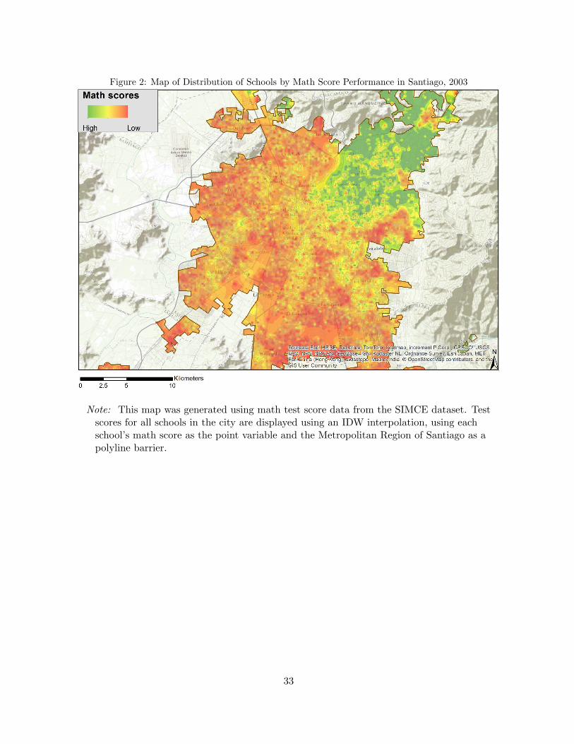
Figure 2: Map of Distribution of Schools by Math Score Performance in Santiago, 2003

Note: This map was generated using math test score data from the SIMCE dataset. Testscores for all schools in the city are displayed using an IDW interpolation, using eachschool’s math score as the point variable and the Metropolitan Region of Santiago as apolyline barrier.

33

Figure 3: Map of Percentage of Students Attending School in Their Own Municipality in 2003

Note: This map was generated using official student registration data from the Ministry ofEducation. I aggregated data for each municipality and then calculated how many of thestudents living there were also attending schools inside the same area.

34

Figure 4: Subway Network in 2006 After the Inauguration of Line 4

Note: I generated this map by geocoding the exact location of each subway station thatexisted at the beginning of 2006, as informed by Metro de Santiago. The subway networkhas since been expanded in recent years with both the inauguration of new lines, and theextension of existing lines.

35

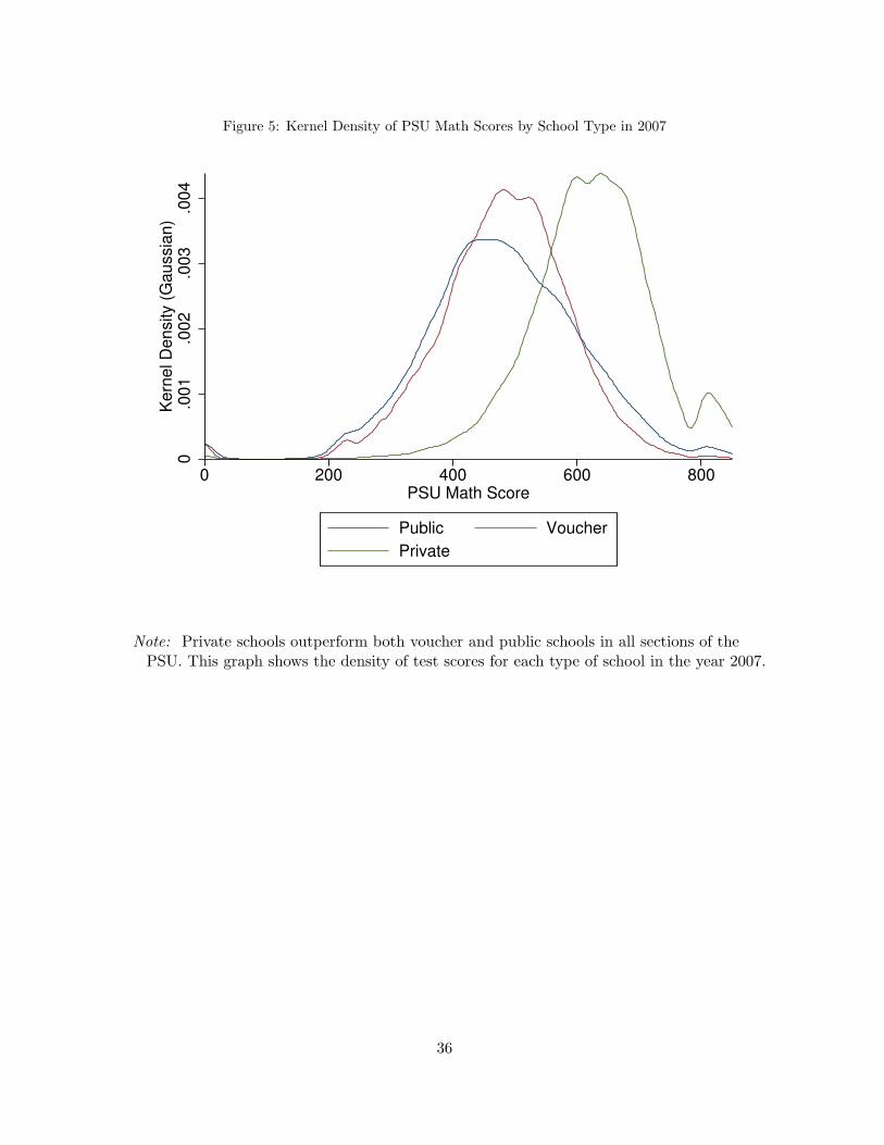
Figure 5: Kernel Density of PSU Math Scores by School Type in 2007

0.0

01

.002

.003

.004

Kern

el D

ensity (

Gaussia

n)

0 200 400 600 800PSU Math Score

Public Voucher

Private

Note: Private schools outperform both voucher and public schools in all sections of thePSU. This graph shows the density of test scores for each type of school in the year 2007.

36

Figure 6: Map of Treated and Control Groups

Note: I generated this map by geocoding the exact location of each high school senior us-ing addresses from PSU registration forms and aggregating them in a fishnet of rectan-gular cells. Students considered as treated by the subway are represented by light greencells, while students that are part of the control group are shown in dark green.

37

Figure

7:Trendsof

CovariatesBetween2003

and2007

(a)Percentage

AttendingPublicSchool

(b)AverageGPA

(c)AverageDistance

toClosest

School

(d)Number

ofSchools

within

a1-km

RadiusFrom

Home

38

Figure 8: Average Distance Traveled to School by Year Between 2003 and 2007

Note: This chart is generated using data from PSU registration forms and SIMCEdatasets. Each data point represents the average distance traveled from home to schoolby students either in the treatment or the control group on a particular year.

39

Figure 9: Distance to Chosen School and Rank-Distance of Chosen School in 2003

0500

1,0

00

1,5

00

Rank−

Dis

tance o

f C

hosen S

chool

0 5,000 10,000 15,000Distance to Chosen School (meters)

Note: This figure shows the relationship between rank-distance to school and distance toschool in meters for the year 2003.

40

Figure 10: Distance to Chosen School and Rank-Distance of Chosen School in 2007

0500

1,0

00

1,5

00

Rank−

Dis

tance o

f C

hosen S

chool

0 5,000 10,000 15,000Distance to Chosen School (meters)

Note: This figure shows the relationship between rank-distance to school and distance toschool in meters for the year 2007.

41

Figure 11: Rank-Distance to School by Year Between 2003 and 2007

Note: This chart is generated using data from PSU registration forms and SIMCEdatasets. Each data point represents the average rank-distance of the chosen school rel-ative to a student’s home for students either in the treatment or the control group on aparticular year.

42

Figure 12: Map of Placebo Subway Lines

Note: I generated this map by offsetting the latitude of the subway line that was inaugu-rated in 2006. I did this several times to generate alternative placebo subway lines to usein falsification tests. This map displays three of those subway lines.

43

Table 1: Percentage of Students that Study in Their Own Municipality Per Year Between 2003 and2007

%

2003 70.52005 71.82007 70.3

Note: This table is generated using data from the Ministry of Education for all students in Santiagoduring the years 2003, 2005 and 2007. I first calculate how many students are going to school in theirown municipalities and show yearly averages of this value.

44

Table 2: Number of Schools in Santiago Per Year Between 2003 and 2007

Private Public Voucher Total

N % N % N % N %

2003 361 17.1 683 32.3 1,072 50.7 2,116 100.02004 325 15.2 681 31.8 1,138 53.1 2,144 100.02005 326 14.7 687 30.9 1,208 54.4 2,221 100.02006 326 14.4 678 29.9 1,267 55.8 2,271 100.02007 329 14.1 680 29.2 1,323 56.7 2,332 100.0

Note: Data used to construct this table comes from the SIMCE dataset. Each set ofcolumns presents the number and percentage of schools for a particular year that corre-sponded to either private, public or voucher schools. The total number of schools in thecity is displayed in the last set of columns.

45

Table 3: Number of High-School Seniors by Type of School in Santiago per Year Between 2003 and2007

Private Public Voucher Total

N % N % N % N %

2003 9,339 23.3 11,705 29.2 19,049 47.5 40,093 100.02004 9,176 22.3 11,543 28.1 20,349 49.5 41,068 100.02005 9,596 20.9 12,396 27.0 23,852 52.0 45,844 100.02006 9,811 17.9 15,765 28.7 29,296 53.4 54,872 100.02007 8,339 16.9 14,175 28.7 26,940 54.5 49,454 100.0

Note: These values correspond to the number of students that were accurately geocodedand thus used in this study, and do not correspond exactly to the total number of stu-dents in Santiago’s school system. Data comes from PSU registration forms. Each set ofcolumns presents the number of high-school seniors attending each type of school.The to-tal number of high-school seniors in the city is displayed in the last set of columns.

46

Table 4: Number of Subway Users Per Year Between 2003 and 2007

2003 2004 2005 2006 2007

Line 1 130,749,000 145,192,992 158,254,000 167,192,000 256,036,992Line 2 34,311,000 39,508,000 51,839,000 58,893,000 120,468,000Line 4 0 0 2,692,000 48,419,000 114,008,000Line 5 38,218,000 47,062,000 54,317,000 53,213,000 89,385,000

Note: There are 0 riders in Line 4 during 2003 and 2004 since it was inaugurated duringthe last months of 2005. Data comes from Metro de Santiago.

47

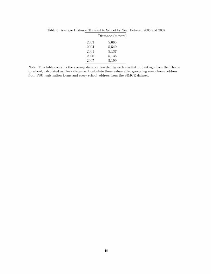
Table 5: Average Distance Traveled to School by Year Between 2003 and 2007

Distance (meters)

2003 5,6652004 5,5492005 5,1372006 5,1362007 5,199

Note: This table contains the average distance traveled by each student in Santiago from their hometo school, calculated as block distance. I calculate these values after geocoding every home addressfrom PSU registration forms and every school address from the SIMCE dataset.

48

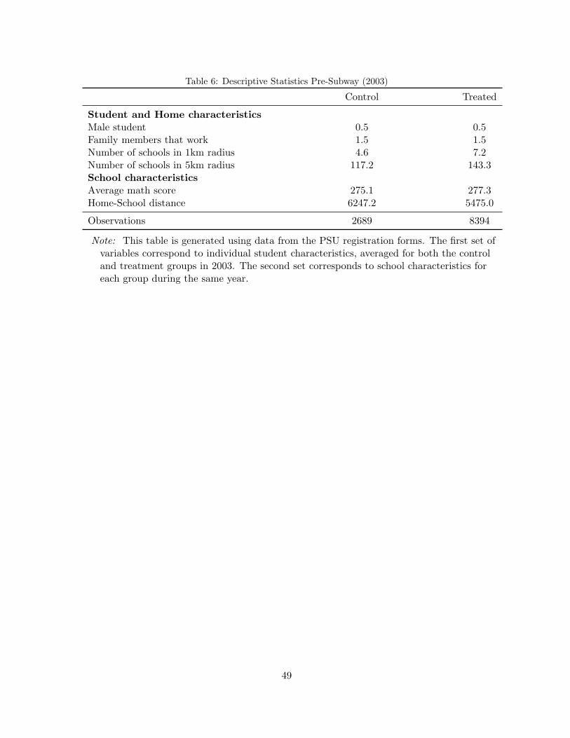
Table 6: Descriptive Statistics Pre-Subway (2003)

Control Treated

Student and Home characteristics

Male student 0.5 0.5Family members that work 1.5 1.5Number of schools in 1km radius 4.6 7.2Number of schools in 5km radius 117.2 143.3School characteristics

Average math score 275.1 277.3Home-School distance 6247.2 5475.0

Observations 2689 8394

Note: This table is generated using data from the PSU registration forms. The first set ofvariables correspond to individual student characteristics, averaged for both the controland treatment groups in 2003. The second set corresponds to school characteristics foreach group during the same year.

49

Table 7: Descriptive Statistics Post-Subway (2007)

Control Treated

Student and Home characteristics

Male student 0.5 0.5Family members that work 1.3 1.3Number of schools in 1km radius 4.6 7.0Number of schools in 5km radius 116.8 141.5School characteristics

Average math score 271.4 271.8Home-School distance 5332.6 5152.8

Observations 3011 8854

Note: This table is generated using data from the PSU registration forms. The first set ofvariables correspond to individual student characteristics, averaged for both the controland treatment groups in 2007. The second set corresponds to school characteristics foreach group during the same year.

50

Table 8: Regression Results (DID): The Effect of Subway Access on Distance Traveled to School

Distance Log distance Rank-Distance

(1) (2) (3) (4) (5) (6)

Access to subway 592.417*** 609.691*** 0.200*** 0.200*** 24.225** 27.118***(168.404) (159.826) (0.035) (0.033) (9.416) (8.908)

Observations 22,046 22,046 22,046 22,046 22,046 22,046R2 0.004 0.103 0.004 0.098 0.002 0.108Controls No Yes No Yes No Yes

Note: Each set of columns presents the results of a separate regression, one for each out-come variable. Columns (2), (4) and (6) present results controlling for the following vari-ables: gender of the student, number of family members that are working, number ofschools in a 1-km radius from the student’s home, number of schools in a 5-km radiusfrom the student’s home, and dummy variables for the type of school.

* p <0.1, ** p <0.05, *** p <0.01. Standard errors in parentheses.

51

Table 9: Regression Results (DID): The Effect of Subway Access on Distance Traveled to School WithFull Covariates

Distance Log distance Rank-Distance

(1) (2) (3)

Access to subway 609.691*** 0.200*** 27.118***(159.826) (0.033) (8.908)

Year after 2006 dummy -903.823*** -0.221*** -45.090***(138.642) (0.029) (7.728)

Treatment dummy -341.590*** -0.072*** -25.142***(122.206) (0.025) (6.811)

Male student 442.328*** 0.066*** 25.813***(69.304) (0.014) (3.863)

Family works -55.022 0.002 -4.245*(45.670) (0.010) (2.546)

Schools close (1km) -131.383*** -0.055*** -5.027***(10.813) (0.002) (0.603)

Schools close (5km) -7.169*** -0.000 0.755***(1.350) (0.000) (0.075)

Public 3921.191*** 0.679*** 229.027***(100.525) (0.021) (5.603)

Voucher 229.078*** -0.002 13.058***(86.428) (0.018) (4.817)

Constant 6538.790*** 8.353*** 104.177***(204.759) (0.043) (11.413)

Observations 22,046 22,046 22,046R2 0.103 0.098 0.108

Note: This table displays the coefficients of all covariates included when estimating equa-tion (1). Each column presents the results of a separate regression, one for each outcomevariable.

* p <0.1, ** p <0.05, *** p <0.01. Standard errors in parentheses.

52

Table 10: Regression Results (DID): The Effect of Subway Access on School Test Scores

Distance Log distance Rank-Distance

(1) (2) (3) (4) (5) (6)

School quality 12.129** 12.165*** 0.002** 0.002** 0.441 0.441*(4.862) (4.575) (0.001) (0.001) (0.271) (0.254)

Observations 22,044 22,044 22,044 22,044 22,044 22,044R2 0.012 0.125 0.007 0.107 0.013 0.135Controls No Yes No Yes No Yes

Note: Each set of columns presents the results of a separate regression, one for each out-come variable. Columns (2), (4) and (6) present results controlling for the following vari-ables: gender of the student, number of family members that are working, number ofschools in a 1-km radius from the student’s home, number of schools in a 5-km radiusfrom the student’s home, and dummy variables for the type of school.

* p <0.1, ** p <0.05, *** p <0.01. Standard errors in parentheses.

53

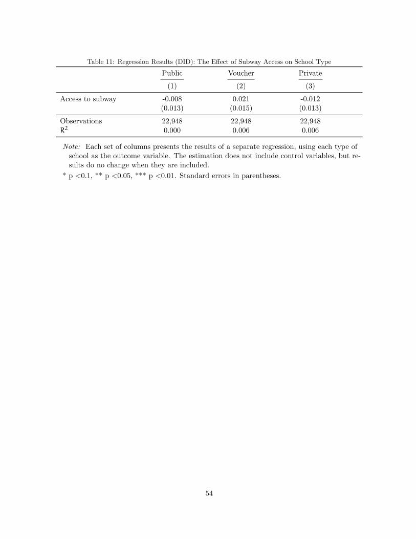
Table 11: Regression Results (DID): The Effect of Subway Access on School Type

Public Voucher Private

(1) (2) (3)

Access to subway -0.008 0.021 -0.012(0.013) (0.015) (0.013)

Observations 22,948 22,948 22,948R2 0.000 0.006 0.006

Note: Each set of columns presents the results of a separate regression, using each type ofschool as the outcome variable. The estimation does not include control variables, but re-sults do no change when they are included.

* p <0.1, ** p <0.05, *** p <0.01. Standard errors in parentheses.

54

Table 12: Regression Results (DID): The Effect of Subway Access on Distance Traveled to School by School Type

Distance Log Distance Rank-Distance

(1) (2) (3) (4) (5) (6) (7) (8) (9)Public Voucher Private Public Voucher Private Public Voucher Private

Access to subway 43.499 760.222*** 821.139*** 0.043 0.247*** 0.233*** -5.983 39.016*** 33.771**(426.483) (205.720) (267.293) (0.069) (0.048) (0.067) (24.729) (10.927) (15.046)

Observations 5,323 11,573 5,150 5,323 11,573 5,150 5,323 11,573 5,150R2 0.006 0.003 0.010 0.005 0.003 0.016 0.005 0.003 0.001

Note: Each set of columns presents the results of a separate regression, one for each outcome variable.Within each set, separate results are presented for each type of school: public, voucher or private. Theestimation does not include control variables, but results do no change when they are included.

* p <0.1, ** p <0.05, *** p <0.01. Standard errors in parentheses.

55

Table 13: Regression Results (DID): The Effect of Subway Access on PSU Math Score

Low Medium High

(1) (2) (3)

Access to subway 0.020 0.004 -0.024*(0.014) (0.015) (0.015)

Observations 22,948 22,948 22,948R2 0.004 0.002 0.001

Note: Each set of columns presents the results of a separate regression, using performancein the PSU math test as the outcome variable, classified as either low, medium or high.The estimation does not include control variables, but results do no change when they areincluded.

* p <0.1, ** p <0.05, *** p <0.01. Standard errors in parentheses.

56

Table 14: Regression Results (DID): The Effect of Subway Access on Distance Traveled to School Us-ing Various Treatment and Control Group Definitions

Distance Distance Distance

(1) (2) (3) (4) (5) (6)

Access to subway 1.5 km 414.425*** 429.543***(155.896) (148.024)

Access to subway 2 km 450.839*** 484.607***(143.367) (136.246)

Access to subway 3 km 663.510*** 767.438***(181.354) (172.204)

Observations 18,952 18,952 23,344 23,344 23,344 23,344R2 0.004 0.103 0.005 0.103 0.004 0.103

(1) (2) (3) (4) (5) (6)

Controls No Yes No Yes No Yes

Note: Each set of columns presents the results of a separate regression, using different def-initions of the treatment and control groups, with distance from home to school as theoutcome variable. Columns (2), (4) and (6) present results controlling for the followingvariables: gender of the student, number of family members that are working, numberof schools in a 1-km radius from the student’s home, number of schools in a 5-km radiusfrom the student’s home, and dummy variables for the type of school.

* p <0.1, ** p <0.05, *** p <0.01. Standard errors in parentheses.

57

Table 15: Regression Results (DID): The Effect of Subway Access on Distance Traveled to School Us-ing Data Before the Subway Line Opened

Distance Log distance Rank-Distance

(1) (2) (3) (4) (5) (6)

Access to subway 144.956 92.504 0.021 0.007 4.321 3.283(176.365) (164.424) (0.037) (0.034) (9.986) (9.299)

Observations 21,208 21,208 21,208 21,208 21,208 21,208R2 0.003 0.134 0.005 0.135 0.000 0.134

(1) (2) (3) (4) (5) (6)

Controls No Yes No Yes No Yes

Note: Each set of columns presents the results of a separate regression, one for each out-come variable. Only the years before the subway line was constructed are considered.Columns (2), (4) and (6) present results controlling for the following variables: genderof the student, number of family members that are working, number of schools in a 1-kmradius from the student’s home, number of schools in a 5-km radius from the student’shome, and dummy variables for the type of school.

* p <0.1, ** p <0.05, *** p <0.01. Standard errors in parentheses.

58

Table 16: Regression Results (DID): The Effect of Subway Access on Distance Traveled to School(Placebo Line 1)

Distance Log distance Rank-Distance

(1) (2) (3) (4) (5) (6)

Access to subway -74.009 -86.941 -0.031 -0.029 -1.688 -1.286(126.510) (122.160) (0.029) (0.028) (7.746) (7.573)

Observations 22,185 22,185 22,185 22,185 22,185 22,185R2 0.000 0.068 0.000 0.083 0.000 0.045Controls No Yes No Yes No Yes

Note: Each set of columns presents the results of a separate regression, one for each out-come variable. Columns (2), (4) and (6) present results controlling for the following vari-ables: gender of the student, number of family members that are working, number ofschools in a 1-km radius from the student’s home, number of schools in a 5-km radiusfrom the student’s home, and dummy variables for the type of school.

* p <0.1, ** p <0.05, *** p <0.01. Standard errors in parentheses.

59

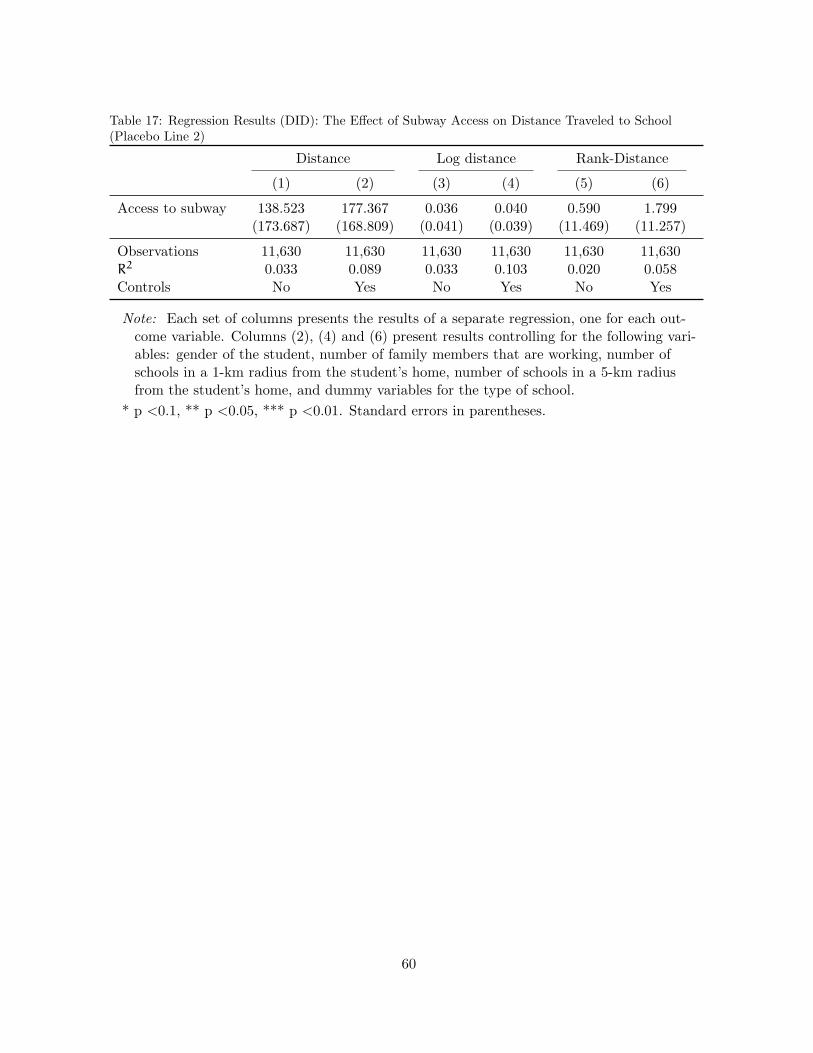
Table 17: Regression Results (DID): The Effect of Subway Access on Distance Traveled to School(Placebo Line 2)

Distance Log distance Rank-Distance

(1) (2) (3) (4) (5) (6)

Access to subway 138.523 177.367 0.036 0.040 0.590 1.799(173.687) (168.809) (0.041) (0.039) (11.469) (11.257)

Observations 11,630 11,630 11,630 11,630 11,630 11,630R2 0.033 0.089 0.033 0.103 0.020 0.058Controls No Yes No Yes No Yes

Note: Each set of columns presents the results of a separate regression, one for each out-come variable. Columns (2), (4) and (6) present results controlling for the following vari-ables: gender of the student, number of family members that are working, number ofschools in a 1-km radius from the student’s home, number of schools in a 5-km radiusfrom the student’s home, and dummy variables for the type of school.

* p <0.1, ** p <0.05, *** p <0.01. Standard errors in parentheses.

60

Table 18: Regression Results (DID): The Effect of Subway Access on Distance Traveled to School(Placebo Line 3)

Distance Log distance Rank-Distance

(1) (2) (3) (4) (5) (6)

Access to subway 223.712 174.774 0.089 0.098 1.965 2.693(392.237) (375.350) (0.098) (0.093) (25.498) (25.039)

Observations 4,732 4,732 4,732 4,732 4,732 4,732R2 0.004 0.091 0.004 0.103 0.000 0.039Controls No Yes No Yes No Yes

Note: Each set of columns presents the results of a separate regression, one for each out-come variable. Columns (2), (4) and (6) present results controlling for the following vari-ables: gender of the student, number of family members that are working, number ofschools in a 1-km radius from the student’s home, number of schools in a 5-km radiusfrom the student’s home, and dummy variables for the type of school.

* p <0.1, ** p <0.05, *** p <0.01. Standard errors in parentheses.

61