The Effect of Economic Transfers on Psychological Well-Being

and Mental Health *

Jimena Romero1 Kristina Esopo2 Joel McGuire3

Johannes Haushofer1,4,5

1Stockholm University2University of California, Santa Barbara

3Happier Lives Institute4Institute for Industrial Economics

5Max-Planck-Institute for Collective Goods

This version: September 14, 2021

Abstract

Transfers of cash or other economic interventions have received renewed attention from policy-makers, philanthropists, academics, and the general public in recent years. We conducted a system-atic review and meta-analysis on the causal impact of economic interventions on psychological well-being and mental health. We reviewed 1,640 abstracts and 127 full-text papers to obtain a final sampleof 57 studies containing 253 treatment effects. We distinguish between different economic interven-tions (conditional and unconditional cash transfers, poverty graduation programs, asset transfers,housing vouchers, health insurance provision, and lottery wins) and different well-being outcomes(depression, stress or anxiety, and happiness or life satisfaction). The average intervention is worthUSD 540 PPP, and impacts on well-being are measured two years after the intervention on average.We find that economic interventions have a positive effect on well-being: on average, an interven-tion increased well-being by 0.100 standard deviations (SD). We observe the largest impacts for assettransfers (0.158 SD) and unconditional cash transfers (0.150 SD). Effects decay over time, and do notdiffer substantially when transfers are directed to men vs. women. We conclude that economic in-terventions have significant potential to improve the psychological well-being and mental health ofrecipients.

*We thank Magdalena Larreboure for excellent research assistance, and Miranda Wolpert and Cat Sebastian for comments.All errors are our own. This work was funded by a Wellcome Trust Mental Health Priority Area ‘Active Ingredients’ commissionawarded to Johannes Haushofer.

1

1. Introduction

According to WHO estimates, mental illnesses are amongst the most important sources of disease bur-

den in the world. Mental illness is strongly linked to poverty in cross-sectional analyses: low-income in-

dividuals have significantly higher rates of mental illness than wealthier individuals (Bromet et al. 2011;

Lund et al. 2010). This correlational result raises the question whether there is a causal relationship, po-

tentially bi-directional, between poverty and mental health. In the public health literature, these twin

hypotheses are referred to as “social causation” (poverty causes mental illness) and “social drift” (mental

illness causes poverty). However, causal evidence on these relationships, and their magnitude, has been

scant.

In recent years, policy makers, philanthropists, academics, and the general public have re-discovered

direct transfers to low-income individuals as a powerful tool of poverty alleviation. These transfers take

various forms, ranging from unconditional and conditional cash transfers to in-kind transfers, e.g. of

food, to transfers of services such as insurance or training. A growing number of studies has investigated

the impact of such transfers on welfare outcomes. Often, the outcomes of interest are economic in na-

ture, including e.g. consumption, asset holdings, and labor supply. However, more recently, researchers

have increasingly turned their attention to the impact of these interventions on psychological well-being

and mental health.

The purpose of the present systematic review is to synthesize the evidence on the impact of eco-

nomic transfers on mental health and subjective well-being. We focus on studies that meet the following

criteria: first, the study has to use randomized assignment of transfers to identify causal effects. There

are two study categories in our sample which meet this criterion: randomized controlled trials (RCTs),

and studies of lottery wins. Second, the intervention has to consist of an economic transfer, which we

define as a transfer of money, goods, or services to individuals without a requirement for repayment.

Note that this definition is relatively broad in that it includes not just cash transfers, but also, for exam-

ple, asset transfers, free provision of insurance, and housing vouchers. Third, the study has to measure

the impact of this intervention on an aspect of mental health or subjective well-being, including, for ex-

ample, depression, happiness, or life satisfaction. (In the following, we use “well-being” as a summary

term for brevity.) We do not restrict the geographic location of the studies, although many are conducted

in low-income countries, or have low-income individuals as participants. Due to the relative paucity of

studies targeting specific age groups, we also do not restrict the age of the recipients.

Using a systematic, pre-registered search strategy, we screened over 1,600 abstracts from published

and unpublished research papers in economics, psychology, medical science, and other disciplines. We

then reviewed the full-text of 127 papers and extracted information about the intervention – such as its

monetary value – and its effect on measures of well-being. We conduct a meta-analysis on the resulting

dataset, which contains 57 papers and 253 treatment effects.

We observe moderately sized and statistically significant positive effects of economic transfers on

measures of well-being. The median intervention in our sample of studies makes a transfer worth USD

540, and thereby generates an improvement in well-being of 0.100 standard deviations (SD) two years

after the intervention. Asset transfers and unconditional cash transfers have the largest impact on well-

2

being (0.158 SD and 0.150 SD, respectively). There is no clear relationship between effect size and transfer

magnitude, possibly due to heterogeneity in samples. We do not find differential effects when transfers

are made to men vs. women, and when they are made as lump-sums or in installments. Transfers in low-

and middle-income countries (LMICs) have a larger effect on average (0.115 SD) than in high-income

countries (0.067 SD). However, this difference is partly due to the different composition of interventions,

in which unconditional cash transfers and asset transfers, interventions with larger impacts, are more

prevalent in LMIC.

Our paper contributes to a set of reviews and meta-analyses on the relationship between economic

and psychological outcomes (Lund et al. 2010; Lund et al. 2011; Ridley et al. 2020). Most closely related

is a recent systematic review and meta-analysis about the effect of cash transfers on psychological well-

being in low- and middle-income countries (McGuire, Kaiser, and Bach-Mortensen 2020). This meta-

analysis reports an average treatment effect of cash transfers on psychological well-being of 0.100 SD.

Our study extends this work beyond cash transfers to include other types of economic transfers, and

beyond low- and middle-income countries.

2. Methods

2.1 Search strategy

In June 2020, a systematic review protocol was registered with the international prospective register

of systematic reviews, PROSPERO, with registration ID number CRD42020189558. We used three ap-

proaches to identify both published and unpublished studies (working papers, technical reports) that

met our selection criteria. First, we conducted systematic searches of the electronic databases PubMed

and RePEc. For each database, we used one set of search terms to identify studies on economic trans-

fers, which included “cash transfer”, “cash”, “income”, “lottery”, “graduation”, “debt relief”, “asset trans-

fer”, and “housing voucher”; and another set of search terms to identify studies on mental health and

psychological well-being, which included “mental health”, “depression”, “psychological”, “well(-)being”,

“happiness”, and “life satisfaction”. To restrict results to randomized controlled trials, we used the option

to restrict results to randomized studies in PubMed. RePEc does not provide an option to restrict results

to RCTs, and we therefore included an additional set of search terms to identify randomized studies, in-

cluding “randomized”, “RCT”, and “trial”. Because lottery wins are not typically examined through RCTs,

we conducted an additional identical search in PubMed and RePEc to ensure the inclusion of these types

of transfers without the restriction to an RCT design. Our second approach was to screen the reference

lists of studies identified in these searches for relevant papers. Finally, we identified a small number

of high-profile researchers who have published on this topic and searched their websites for relevant

papers.

3

2.2 Selection criteria

We aimed to include randomized controlled trials (RCTs) and lottery studies which report treatment

effects on any aspect of mental health or subjective well-being, including, for example, depression, hap-

piness, or life satisfaction.

For the initial search, two reviewers (KE, JR) used a software called abstrackr to independently screen

abstracts and subsequently accept or reject each study for full text review. Abstracts were selected for full-

text review if they described (1) an economic transfer intervention, defined as a transfer of money, goods,

or services to individuals without a requirement for repayment; (2) at least one quantitatively measured

mental health or subjective well-being outcome; and (3) an RCT study design or a lottery design.

Subjective well-being outcomes had to fulfill the following criteria: (1) the outcome is measured with

a self-report, i.e. an individual reports their well-being using a Likert or similar scale; in addition, we

include measures of stress hormones, in particular cortisol levels. (2) The self-report elicits feelings or

thoughts about how the individual’s life is going or how they are feeling (emotions, evaluations, moods).

(3) The self-reports elicit broad assessments, rather than assessments restricted to a single domain of

life, such as financial well-being. However, we do accept indices that combine items that cover many do-

mains. Any disagreements regarding the eligibility of particular studies were resolved through discussion

with a third reviewer (JH).

The same two reviewers (KE, JR) independently reviewed the full text of the studies identified in the

abstract screening phase and used a standardized, pre-piloted digital spreadsheet to extract data from

all included studies. The following data were extracted: publication title and authors; study year; coun-

try; description of study population; population age range and/or average; share of female beneficiaries;

type of economic transfer; transfer value in USD; details of the intervention and control conditions, in-

cluding number of participants assigned to each group; delay between intervention and measurement of

outcomes; description of mental health outcomes measured and frequency of measurement; and mag-

nitude of the treatment effect. The extracted data was later reviewed by a third reviewer (JM), and then

used to determine study eligibility for inclusion in the review. Discrepancies between the data extracted

and the final determination to include or exclude a particular study were reconciled by an additional

reviewer (JH).

We classified the interventions into seven categories: unconditional cash transfers (UCTs); condi-

tional cash transfers (CCTs); neighborhood programs (housing vouchers); poverty graduation programs;

lotteries; asset transfers; and insurance provision. Poverty graduation programs are compound interven-

tiosn that typically consist of an asset transfer, training, and a cash transfer. Similarly, we classified the

outcomes into three outcome groups: depression; stress or anxiety; and happiness or life satisfaction.

Depression outcomes included the Center for Epidemiological Studies Depression Scale (CES-D), the

Geriatric Depression Scale, the John Hopkins Depression Checklist, and the Symptom-Driven Diagnos-

tic System for Primary Care. The CES-D was the most common. Measures of stress and anxiety included

the Kessler Psychological Distress Scale (K6), cortisol levels, the General Health Questionnaire (GHQ),

and Cohen’s Perceived Stress Scale, with the K6 being the most common. Happiness and life satisfaction

included measures of self-reported happiness, life satisfaction, subjective well-being, and unhappiness,

4

such as the Gallup Q-12 index, the most common being self-reported happiness.

We excluded outcomes that did not correspond to any of these groups, such as cognitive outcomes

or anti-social behaviors. We also extracted treatment effects on index variables that summarize several

mental health measures; however, to avoid double-counting outcomes, we do not include these variables

in our meta-analysis.

The search followed PRISMA guidelines, and an overview of the process is shown in Figure 1. From

1,640 abstracts returned from the search strategy, 127 were chosen for full-text review in the screening

process. Fifty-four of these papers were excluded after full-text review because they did not meet the

inclusion criteria, and 16 because they did not contain sufficient information to compute standardize

treatment effects. From the remaining 57 papers, we extracted treatment effects for every mental health

index and component reported. Thus, if a study reported treatment effects for more than one outcome

variable, or more than one treatment, they were extracted separately1. This yielded 57 papers with 253

treatment effects to be analyzed.

1. To avoid double counting, we did not include general indexes of mental health well-being if more specific outcomes wereextracted

5

Figure 1: PRISMA diagram for study selection and inclusion

6

2.3 Data analysis

2.3.1 Standardization

To make treatment effects comparable across studies, we began by standardizing them, i.e. converting

them into standard deviation (z-score) units. This is accomplished by dividing the treatment effect with

the standard deviation of the control group at endline. This is the correct standard deviation to use for the

same reasons that the average outcomes of the control group at endline are the correct counterfactual

for the treatment effect itself. Where the standard deviation of the control group at endline was not

available, we estimated it as follows:

(1) We check if the treatment effect is already standardized. In this case, we use this standardized

treatment effect (thereby adopting the standardization method of the paper, even if it differs from our

preferred approach). (2) If the treatment effect is not standardized, we check if the paper reports the stan-

dard deviation of the control group at the endline, in which case we use it to perform the standardiza-

tion. (3) If this value is not available, we check if the outcome is continuous or binary. (4) If the outcome

is binary, we check whether the share p of individuals responding affirmatively in the control group is

reported. In this case, we compute the control group standard deviation using the formulate for the stan-

dard deviation of a proportion, SD =√p(1−p). If the share of affirmative responses in the control group

at endline is not reported, we use baseline information if available. (5) If the outcome is continuous and

the study reports sample sizes and the standard error of the treatment effect, we approximate the stan-

dard deviation of the control group using the t-test formula, assuming equal variances for the control

and treatment groups. Specifically, the t-test formula for a difference in means is t = x̄1−x̄2SE = x̄1−x̄2√

SD21

n1+ SD2

2n2

.

Assuming equal variances SD2 = SD21 = SD2

2 in both groups, we can calculate the SD as a function of the

standard error and sample sizes: SD =√

SE 2n1n2n1+n2

, where n1 and n2 are the sample sizes of the treatment

and control groups, respectively. The standard error of the treatment effect was standardized in the same

fashion as the treatment effects.

Prior to the standardization, all “negative” outcomes, such as stress and depression, were re-coded so

that high values correspond to “positive” outcomes (i.e. the absence of stress or depression). All z-scores

were adjusted for small sample sizes using Hedges’ formula.2

2.3.2 Meta-analysis Methods

We analyzed the 253 effect sizes that resulted from our systematic review using a random-effects (RE)

meta-analysis model3, using the Sidik-Jonkman estimator.4 Each effect size gets weighted with the in-

verse of its standard error, thereby giving studies with greater precision more weight.

Because the same study often contributes more than one treatment effect, we use cluster-robust

standard errors at the study level. We run this analysis both for all interventions and outcomes, and

2. Hedges’ adjustment for small sample sizes is z∗ = z × (1− 3(4n1+4n2−9 ).

3. Random effect models assume that true effects of each study are drawn from a distribution of true effects (Borenstein etal. 2010), while fixed effects (FE) models assume that all included studies share a common true effect.

4. Results are similar when we use alternative random effects estimators; see Figure A1.

7

separately for each intervention type and outcome. In addition, we run the analysis once for the sample

as a whole, and for the subsets of low-/middle-income countries and high-income countries.

To assess the relationship between effect sizes and various characteristics of the interventions and

beneficiaries, we additionally estimate a meta-regression in which we include the following variables on

the right-hand side: average age of the participants (or, where average age is not available, midpoint of

the age range); intervention value as percentage of per-capita GDP in the study country, measured in

1,000s of USD; average delay between intervention and outcome measurement in years; female share

of the participants (ranging from 0 for all-male samples to 1 for all-female samples); and whether the

intervention was delivered as a lump-sum transfer or in repeated installments. Specifically, we estimate:

θi =β0 +β1 Ag ei +β2LM ICi +β3Femal ei +β4Lumpsumi +β5V aluei +β6Y ear si +εi

We again run this analysis both for all interventions and outcome measures, and separately for each

type of intervention and outcome measure.

Finally, we examine evidence of publication bias with three adjustment methods: Vevea and Hedges

1995; Aert and Assen 2018; and Andrews and Kasy 2019. See Appendix A2 for further information on

these methods.

3. Results

3.1 Study Overview

Our final sample of 57 studies consists of 27 studies of unconditional cash transfers,5 6 of conditional

cash transfers,6 11 of housing vouchers,7 6 of lotteries,8 3 of graduation programs and other multifaceted

interventions such as enterprise development programs,9 3 of asset transfers,10 and 3 of insurance pro-

vision.1112

An overview of studies and their characteristics is shown in Table 1, which shows for each study: (1)

the intervention type (unconditional cash transfer, conditional cash transfer, insurance provision, hous-

ing voucher, asset transfer, lottery, or poverty graduation program); (2) the average transfer value; (3) the

classification of the outcomes measured; (4) the delay between the time of the start of the intervention

5. Alzua et al. 2020; Angeles et al. 2019; Baird, Hoop, and Özler 2013; Bando, Galiani, and Gertler 2020; Ahbijit Banerjee etal. 2020; Blattman, Fiala, and Martinez 2011, 2014; Blattman, Jamison, and Sheridan 2017; Blattman, Fiala, and Martinez 2019;Egger et al. 2019; Fernald and Hidrobo 2011; Ferrah and Mvukiyehe, n.d.; Green et al. 2016; Haushofer and Shapiro 2016, 2018;Haushofer, Mudida, and Shapiro 2019, 2020; Heath, Hidrobo, and Roy 2020; Hjelm et al. 2017; Kilburn et al. 2018; McIntoshand Zeitlin 2020; Molotsky and Handa 2021; Muller, Pape, and Ralston 2019; Natali et al. 2018; Paxson and Schady 2010; Royet al. 2019; Stein et al. 2020

6. Baird, Hoop, and Özler 2013; Blattman, Fiala, and Martinez 2019; Kilburn et al. 2019; Macours, Schady, and Vakis 2012;Morris et al. 2017; Ohrnberger et al. 2020

7. Andersen, Kotsadam, and Somville 2021; Fauth, Leventhal, and Brooks-Gunn 2004; Katz, Kling, and Liebman 2001; Kessleret al. 2014; Kling, Liebman, and Katz 2007; Leventhal and Brooks-Gunn 2003; Leventhal and Dupéré 2011; Ludwig et al. 2013;Nguyen et al. 2013; Osypuk et al. 2012; Sanbonmatsu et al. 2011

8. Burger et al. 2020; Gardner and A. Oswald 2001; Gardner and A. J. Oswald 2007; Kim and Oswald 2021; Kuhn et al. 2011;Lindqvist, Östling, and Cesarini 2020

9. Abhijit Banerjee et al. 2015; Bossuroy et al. 2021; Ismayilova et al. 201810. Edmonds and Theoharides 2020; Glass et al. 2017; Quattrochi et al. 202011. Baicker et al. 2013; Finkelstein et al. 2012; Haushofer et al. 202012. Some studies are counted doubly because they contain more than one type of economic intervention.

8

and outcome measurement; (5) the target population; (6) the country in which the intervention took

place; and (7) the sample size.

9

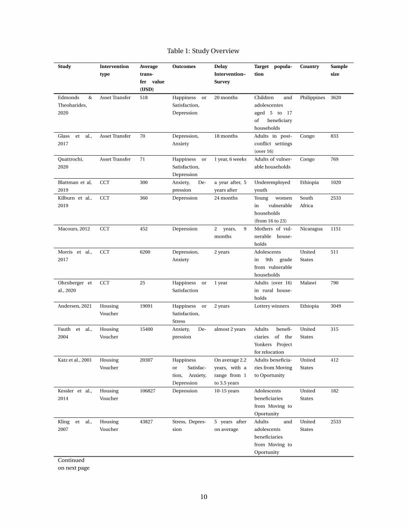
Table 1: Study Overview

Study Intervention

type

Average

trans-

fer value

(USD)

Outcomes Delay

Intervention–

Survey

Target popula-

tion

Country Sample

size

Edmonds &

Theoharides,

2020

Asset Transfer 518 Happiness or

Satisfaction,

Depression

20 months Children and

adolescentes

aged 5 to 17

of beneficiary

households

Philippines 3620

Glass et al.,

2017

Asset Transfer 70 Depression,

Anxiety

18 months Adults in post-

conflict settings

(over 16)

Congo 833

Quattrochi,

2020

Asset Transfer 71 Happiness or

Satisfaction,

Depression

1 year, 6 weeks Adults of vulner-

able households

Congo 769

Blattman et al,

2019

CCT 300 Anxiety, De-

pression

a year after, 5

years after

Underemployed

youth

Ethiopia 1020

Kilburn et al.,

2019

CCT 360 Depression 24 months Young women

in vulnerable

households

(from 16 to 23)

South

Africa

2533

Macours, 2012 CCT 452 Depression 2 years, 9

months

Mothers of vul-

nerable house-

holds

Nicaragua 1151

Morris et al.,

2017

CCT 6200 Depression,

Anxiety

2 years Adolescents

in 9th grade

from vulnerable

households

United

States

511

Ohrnberger et

al., 2020

CCT 25 Happiness or

Satisfaction

1 year Adults (over 16)

in rural house-

holds

Malawi 790

Andersen, 2021 Housing

Voucher

19091 Happiness or

Satisfaction,

Stress

2 years Lottery winners Ethiopia 3049

Fauth et al.,

2004

Housing

Voucher

15400 Anxiety, De-

pression

almost 2 years Adults benefi-

ciaries of the

Yonkers Project

for relocation

United

States

315

Katz et al., 2001 Housing

Voucher

20307 Happiness

or Satisfac-

tion, Anxiety,

Depression

On average 2.2

years, with a

range from 1

to 3.5 years

Adults beneficia-

ries from Moving

to Oportunity

United

States

412

Kessler et al.,

2014

Housing

Voucher

106827 Depression 10-15 years Adolescents

beneficiaries

from Moving to

Oportunity

United

States

182

Kling et al.,

2007

Housing

Voucher

43827 Stress, Depres-

sion

5 years after

on average

Adults and

adolescents

beneficiaries

from Moving to

Oportunity

United

States

2533

Continuedon next page

10

Table 1: Study Overview

Study Intervention

type

Average

trans-

fer value

(USD)

Outcomes Delay

Intervention–

Survey

Target popula-

tion

Country Sample

size

Leventhal &

Brooks-Gunn,

2003

Housing

Voucher

27027 Stress, Depres-

sion

3 years Adults and chil-

dren beneficia-

ries from Moving

to Oportunity

United

States

369

Leventhal &

Dupere, 2011

Housing

Voucher

52227 Stress, Anxiety 5-7 years Adolescents

beneficiaries

from Moving to

Oportunity

United

States

1780

Ludwig et al.,

2013

Housing

Voucher

106827 Depression,

Stress, Hap-

piness or

Satisfaction

10-15 years Adults and

adolescents

beneficiaries

from Moving to

Oportunity

United

States

2595

Nguyen et al.,

2013

Housing

Voucher

48027 Stress 4-7 years Adolescents

beneficiaries

from Moving to

Oportunity

United

States

1426

Osypuk et al.,

2012

Housing

Voucher

48027 Stress 4-7 years Adolescents

beneficiaries

from Moving to

Oportunity

United

States

2829

Sanbonmatsu

et al., 2011

Housing

Voucher

106827 Stress 10-15 years Adults and

adolescents

beneficiaries

from Moving to

Oportunity

United

States

4644

Baicker et al.,

2013

Insurance

Provision

7000 Happiness or

Satisfaction,

Depression

2 years Adults benefi-

ciaries of the

Oregon Health

Insurance exper-

iment

United

States

12229

Finkelstein et

al., 2012

Insurance

Provision

4083 Depression,

Happiness or

Satisfaction

14 months Adults benefi-

ciaries of the

Oregon Health

Insurance exper-

iment

United

States

23741

Haushofer et

al., 2020

Insurance

Provision,

UCT

338 Depression,

Stress, Hap-

piness or

Satisfaction

1 year Metalworkers of

the Kamukunji

Jua Kali Associa-

tion

Kenya 693

Burger et al.,

2020

Lottery 10 Happiness or

Satisfaction

1 week Lottery winners Netherlands 1097

Gardner & Os-

wald, 2001

Lottery 200 Stress, Happi-

ness or Satis-

faction

12 months Lottery winners United

Kingdom

9493

Gardner & Os-

wald, 2007

Lottery 4303 Stress 2 years Lottery winners United

Kingdom

12620

Kim, 2020 Lottery 254 Happiness or

Satisfaction

1 year Lottery winners Singapore 5626

Continuedon next page

11

Table 1: Study Overview

Study Intervention

type

Average

trans-

fer value

(USD)

Outcomes Delay

Intervention–

Survey

Target popula-

tion

Country Sample

size

Kuhn et al.,

2011

Lottery 30000 Happiness or

Satisfaction

6 montths Lottery winners Netherlands 1458

Lindqvist et al.,

2020

Lottery 106000 Happiness or

Satisfaction,

Stress

5 to 22 years Lottery winners Sweden 3331

Banerjee et al.,

2015

Poverty Grad-

uation Pro-

gram

6475 Happiness or

Satisfaction,

Anxiety, Stress

24 months, 36

months

Adults from

ultra-poor

households

Ethiopia,

Ghana,

Hon-

duras,

India,

Pakistan,

Peru

14595

Bossuroy, 2021 Poverty Grad-

uation Pro-

gram

127 Depression,

Happiness or

Satisfaction,

Anxiety, Stress

6 months, 18

months

Women over 20

years old in ex-

treme poverty

Niger 2409

Ismayilova et

al., 2018

Poverty Grad-

uation Pro-

gram

100 Depression 24 months, 12

months

Children (10-15

years) of ultra-

poor households

Burkina

Faso

240

Alzua et al.,

2021

UCT 384 Depression,

Happiness or

Satisfaction

6 months, 1

year

Older adults

over 65 years old

from vulnerable

households

Nigeria 6059

Angeles et al.,

2019

UCT 192 Depression 2 years Young people

from ultra-

poor labor

constrainded

households

Malawi 1366

Bando, 2021 UCT 1104 Depression 1 year Older adults

(over 65) liv-

ing under the

poverty line

Paraguay 1939

Banerjee et al.,

2020

UCT 675 Depression 30 months, 24

months

Adults from poor

households

Kenya 4909

Blattman et al.,

2011

UCT 374 Depression 24-30 months Poor and unem-

ployed adults

aged 16-45

Uganda 1881

Blattman et al.,

2014

UCT 374 Happiness or

Satisfaction

24-30 months,

4 years

Poor and unem-

ployed adults

aged 16-35

Uganda 1996

Blattman et al.,

2017

UCT 200 Depression 2-5 weeks, 12-

13 months

High-risk men

aged 18-35

Liberia 470

Blattman et al.,

2019

UCT 374 Depression,

Stress

9 years Poor and unem-

ployed adults

aged 16-40

Uganda 1868

Egger et al.,

2019

UCT 1000 Depression 11 months Adults from poor

households

Kenya 4121

Continuedon next page

12

Table 1: Study Overview

Study Intervention

type

Average

trans-

fer value

(USD)

Outcomes Delay

Intervention–

Survey

Target popula-

tion

Country Sample

size

Fernald et. al,

2011

UCT 360 Depression 2 years Mothers of vul-

nerable house-

holds

Ecuador 1196

Ferrah, 2021 UCT 227 Happiness or

Satisfaction,

Depression

2 to 2.5 years Women from

vulnerable

households

Tunisia 1356

Green et al.,

2016

UCT 150 Depression 16 months Young people in

post-conflict set-

tings (from 14 to

30 years old)

Uganda 1726

Haushofer &

Shapiro, 2016

UCT 354 Stress, Hap-

piness or

Satisfaction,

Anxiety, De-

pression

9 months Heads of poor

households

Kenya 1474

Haushofer &

Shapiro, 2018

UCT 354 Stress, Hap-

piness or

Satisfaction,

Depression

33 months Heads of poor

households

Kenya 1491

Haushofer et

al., 2019

UCT 485 Happiness or

Satisfaction,

Depression,

Stress

1 year Adults in rural

areas

Kenya 2140

Heath et al.,

2020

UCT 324 Stress 18 months Adults of poor

households with

a child aged 6-23

months

Mali 1143

Hjelm et. al,

2017

UCT 396 Stress 36 months Mothers of poor

households with

a child under 5

Zambia 2490

Kilburn et al.,

2018

UCT 85 Happiness or

Satisfaction

17 months Caregivers

in ultra-

poor, labor-

constrainted

households

Malawi 2919

McIntosh &

Zeitlin, 2020

UCT 750 Depression 15 months Young people

aged 16-30 from

poor house-

holds with less

than secondary

education

Rwanda 666

Molotskya,

2020

UCT 120 Stress, Happi-

ness or Satis-

faction

Combined

Follow up

waves

Caregivers in

vulnerable

households

Malawi 7551

Muller et al.,

2019

UCT 1000 Happiness or

Satisfaction

2.5 years Young people

aged 18 from 34

from vulnerable

households

South Su-

dan

1495

Continuedon next page

13

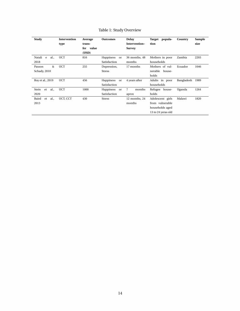
Table 1: Study Overview

Study Intervention

type

Average

trans-

fer value

(USD)

Outcomes Delay

Intervention–

Survey

Target popula-

tion

Country Sample

size

Natali e al.,

2018

UCT 816 Happiness or

Satisfaction

36 months, 48

months

Mothers in poor

households

Zambia 2203

Paxson &

Schady, 2010

UCT 255 Depression,

Stress

17 months Mothers of vul-

nerable house-

holds

Ecuador 1046

Roy et al., 2019 UCT 456 Happiness or

Satisfaction

4 years after Adults in poor

households

Bangladesh 1989

Stein et al.,

2020

UCT 1000 Happiness or

Satisfaction

7 months

aprox

Refugee house-

holds

Uganda 1264

Baird et al.,

2013

UCT, CCT 430 Stress 12 months, 24

months

Adolescent girls

from vulnerable

households aged

13 to 24 yeras old

Malawi 1820

14

3.2 Pooled effect of transfers on mental health and well-being

We extracted 253 treatment effects from these studies. Multiple treatment effects in one study occur

when different interventions are delivered (e.g. large vs. small cash transfers), or when separate treat-

ment effects are reported for different subgroups (e.g. cash transfers to men and women). The average

transfer value is USD 540, and the average delay between intervention and outcome measurement is two

years.

Figure 2 shows the forest plot for the studies included in the paper. If we have more than one outcome

per study, the forest plot presents the pooled estimate13. Table 2 shows the pooled treatment effects

for different kinds of economic interventions and various mental health outcome generated using the

meta-analysis approach described above. Each cell corresponds to a single meta-analysis regression,

and shows the meta-analytic effect size and its standard error.

We find an overall effect of 0.100 SD of any transfer on well-being outcomes, statistically significant at

the 1 percent level. There is some heterogeneity across types of intervention: the largest statistically sig-

nificant treatment effect is observed for asset transfers, which increase measures of well-being by 0.158

SD, significant at the 10 percent level,14, closely followed by unconditional cash transfers, which increase

measures of well-being by 0.150 SD, significant at the 1 percent level. Health insurance provision, stud-

ied in the Oregon Health Insurance Experiment and an RCT in Kenya, improved mental health by 0.093

SD, although this effect is not statistically significant at conventional levels. However, the effects of in-

surance provision are significant for depression and stress/anxiety outcomes. This pattern of results is

driven by a reduction in stress and the stress hormone cortisol in the Kenya study, and by a reduction

in depression in the US study. Poverty graduation programs have a positive but not statistically signif-

icant effect of 0.079 SD. Lotteries had an effect of 0.073 SD, significant at the 10 percent level. Housing

vouchers, studied in an Ethiopian housing lottery, and in two US programs (“Moving to Opportunity”,

and a similar program in New York) have an effect of 0.070 SD, significant at the 1 percent level. Finally,

conditional cash transfer (CCT) programs had an effect of 0.043 SD, significant at the 5 percent level.

Turning to different outcome variables, we observe the largest effect of transfers on happiness (0.131

SD) and depression (0.126 SD), both significant at the 1 percent level. Stress and anxiety show a 0.055 SD

improvement on average, significant at the 1 percent level. The largest overall effects are generated by

UCTs on happiness (0.180 SD), significant at the 1 percent level. Figure 3 presents a comparison of these

effects by intervention type and well-being outcome.

13. The pooled result is estimated using the ’SJ’ method for meta-analysis, weighted by the inverse of the standard error of theoutcome.

14. Note that the concept of significance at the 10 percent level is used in economics, but not psychology and medical science.

15

Figure 2: Forest plot of effects of economic transfers on well-being

Study

Random effects modelHeterogeneity: I2 = 90%, τ2 = 0.0148, p < 0.01

Fernald et. al, 2011Kessler et al., 2014Kuhn et al., 2011Osypuk et al., 2012Nguyen et al., 2013Paxson & Schady, 2010Muller et al., 2019Kim, 2020Blattman et al., 2017Kilburn et al., 2019Lindqvist et al., 2020Macours, 2012Sanbonmatsu et al., 2011Leventhal & Dupere, 2011Blattman et al., 2019Hjelm et. al, 2017Morris et al., 2017Kling et al., 2007Edmonds & Theoharides, 2020Banerjee et al., 2015Ludwig et al., 2013Green et al., 2016Blattman et al, 2019Finkelstein et al., 2012Roy et al., 2019Alzua et al., 2021Baird et al., 2013Fauth et al., 2004Haushofer et al., 2020Andersen, 2021Blattman et al., 2011Natali e al., 2018Haushofer & Shapiro, 2018Ismayilova et al., 2018Banerjee et al., 2020Ohrnberger et al., 2020Gardner & Oswald, 2007Egger et al., 2019Gardner & Oswald, 2001Bossuroy, 2021Baicker et al., 2013Glass et al., 2017Haushofer & Shapiro, 2016Leventhal & Brooks−Gunn, 2003Katz et al., 2001Haushofer et al., 2019Heath et al., 2020Quattrochi, 2020Stein et al., 2020Blattman et al., 2014McIntosh & Zeitlin, 2020Angeles et al., 2019Ferrah, 2021Bando, 2021Molotskya, 2020Kilburn et al., 2018Burger et al., 2020

Treatment Effect

−0.06−0.05−0.01−0.01−0.01−0.010.000.010.020.020.020.020.030.030.030.040.040.040.050.050.050.060.060.060.070.070.070.080.080.080.080.090.090.090.100.110.110.120.120.130.130.130.140.160.160.170.190.200.220.230.260.320.390.480.500.551.30

Standard Error

0.060.280.030.130.120.070.960.000.070.030.010.030.030.040.030.060.090.050.040.010.020.060.030.020.070.020.040.100.040.120.050.020.030.070.020.060.060.070.060.030.060.150.040.040.050.030.120.040.090.030.090.040.350.030.080.140.63

−2 −1 0 1 2

Standardised MeanDifference Intervention Type

UCTHousing VoucherLotteryHousing VoucherHousing VoucherUCTUCTLotteryUCTCCTLotteryCCTHousing VoucherHousing VoucherUCTUCTCCTHousing VoucherAsset TransferPoverty Graduation ProgramHousing VoucherUCTCCTInsurance ProvisionUCTUCTUCT, CCTHousing VoucherInsurance Provision, UCTHousing VoucherUCTUCTUCTPoverty Graduation ProgramUCTCCTLotteryUCTLotteryPoverty Graduation ProgramInsurance ProvisionAsset TransferUCTHousing VoucherHousing VoucherUCTUCTAsset TransferUCTUCTUCTUCTUCTUCTUCTUCTLottery

Country

EcuadorUnited StatesNetherlandsUnited StatesUnited StatesEcuadorSouth SudanSingaporeLiberiaSouth AfricaSwedenNicaraguaUnited StatesUnited StatesUgandaZambiaUnited StatesUnited StatesPhilippinesMultipleUnited StatesUgandaEthiopiaUnited StatesBangladeshNigeriaMalawiUnited StatesKenyaEthiopiaUgandaZambiaKenyaBurkina FasoKenyaMalawiUnited KingdomKenyaUnited KingdomNigerUnited StatesCongoKenyaUnited StatesUnited StatesKenyaMaliCongoUgandaUgandaRwandaMalawiTunisiaParaguayMalawiMalawiNetherlands

Notes: This forest plot shows point estimates and 95% confidence intervals for the main well-being outcome in each of the 57 studies inour sample. The size of each marker corresponds to the study’s sample size, and the color corresponds to the intervention type.

16

Table 2: Meta-analytic estimates of effects of economic transfers on well-being

(1) (2) (3) (4)All Mental Health

Outcomes Depression Stress or Anxiety Happiness

All Interventions 0.100 0.126 0.055 0.131(0.013)*** (0.021)*** (0.010)*** (0.019)***[ 253 / 57 ] [ 89 / 34 ] [ 98 / 28 ] [ 66 / 28 ]

Unconditional Cash Transfer 0.150 0.163 0.081 0.180(0.023)*** (0.039)*** (0.024)** (0.033)***[ 82 / 27 ] [ 39 / 17 ] [ 18 / 10 ] [ 25 / 13 ]

Conditional Cash Transfer 0.043 0.028 0.053 0.106(0.009)** (0.012)* (0.013)* (0.060)*[ 16 / 6 ] [ 8 / 4 ] [ 7 / 3 ] [ 1 / 1 ]

Housing Voucher 0.070 0.104 0.041 0.089(0.001)*** (0.001)** (0.005)** (0.039)[ 66 / 11 ] [ 25 / 6 ] [ 34 / 10 ] [ 7 / 3 ]

Poverty Graduation Program 0.079 0.115 0.047 0.124(0.028) (0.005)** (0.027) (0.040)

[ 51 / 3 ] [ 6 / 2 ] [ 28 / 2 ] [ 17 / 2 ]

Lottery Win 0.073 — 0.082 0.068(0.029)* (0.022)* (0.050)[ 15 / 6 ] [ 0 / 0 ] [ 8 / 3 ] [ 7 / 5 ]

Asset Transfer 0.158 0.137 0.156 0.181(0.048)* (0.057) (0.227) (0.044)[ 12 / 3 ] [ 6 / 3 ] [ 1 / 1 ] [ 5 / 2 ]

Health Insurance Provision 0.093 0.075 0.231 0.092(0.015) (0.001)** (0.067)*** (0.020)

[ 11 / 3 ] [ 5 / 3 ] [ 2 / 1 ] [ 4 / 3 ]

Notes: Meta-analytic estimates for the effect of different types of economic interventions (rows) on dif-ferent well-being outcomes (columns), analyzed using a random effects model. The first row shows theimpact of any intervention on the various well-being outcomes; the remaining rows show the impactof specific interventions. Similarly, the first column reports the effect of interventions on any mentalhealth outcome, while the remaining columns focus on specific outcomes. Standard errors, clusteredat the study level, are shown in parentheses. The number of treatment effects and studies on which theestimate in each cell is based is shown in brackets [number of treatment effects / number of studies].*** denotes significance at the 1 percent level, ** at the 5 percent level, and * at the 10 percent level(note that this convention of denoting significance levels is used in economics but not in psychologyand medicine).

17

Figure 3: Meta-analytic estimates of effects of economic transfers on well-being

Notes: Meta-analytic estimates for the effect of different economic interventions on well-being outcomes. The left panel shows the impacts of any economicintervention on different well-being outcomes; the right panel shows the impacts of different economic interventions on any well-being outcome. Standard

errors represent 95% confidence intervals.

18

3.3 Which variables correlate with effect sizes?

To understand how the observed effect sizes are related to specific characteristics of the intervention or

the participants, we examined five variables: (1) average age of the beneficiaries; (2) a binary variable

indicating if the intervention took place in a low-/middle-income country; (3) the share of female bene-

ficiaries; (4) a binary variable indicating whether the treatment was given as a lump-sum or in repeated

installments; (5) the value of the intervention as a percentage of GDP per capita in the study country;

and (6) the delay in years between the beginning of the transfer and the outcome measurement. Results

by intervention type are show in Table 3, and by outcome in Table 4. We find that effect sizes become

smaller as the delay between intervention and outcome measurement increases; each year decreases the

effect size by 0.006 SD. Perhaps surprisingly, we find no consistent effect of intervention value, possibly

due to the considerable heterogeneity in intervention types and countries. Interventions in low- and

middle-income countries have qualitatively larger effects, but this difference is not statistically signifi-

cant. We observe little variation of effect sizes with age, share of women in the sample, and as a function

of transfer modality (lump-sum vs. installments).

To mitigate the loss of statistical power that results from distinguishing between seven intervention

types, we also conduct an exploratory analysis in which we divide the sample into studies of “in cash” vs.

“in kind” transfers. Results are shown in Table A6. We confirm the finding that effect size decreases over

time. In addition, in-kind transfers have larger effects when they are made to women than to men.

19

Table 3: Correlates of effect size, by intervention type

(1) (2) (3) (4) (5) (6) (7) (8)

AllInterventions

UnconditionalCash

Transfer

ConditionalCash

TransferHousingVoucher

PovertyGraduation

ProgramLottery

WinAsset

Transfer

HealthInsuranceProvision

Constant 0.099 0.134 0.199 0.011 0.163 -7.046 0.209 6.090(0.065) (0.165) (0.129) (0.065) (0.111) (1.801)*** (0.277) (20.999)

Age 0.000 0.001 -0.002 -0.001 -0.001 0.124 -0.010 -0.174(0.001) (0.003) (0.004) (0.002) (0.003) (0.032)*** (0.022) (0.603)

Low-/Middle- 0.032 — 0.062 -2.453 — 0.845 — —Income Country (0.029) (0.118) (3.687) (0.643)

Female Share 0.034 -0.024 -0.153 0.185 0.026 -0.053 0.461 1.342(0.065) (0.059) (0.209) (0.055)*** (0.112) (0.062) (1.050) (5.093)

Lump Sum -0.024 -0.016 0.045 — — — — —(0.036) (0.058) (0.093)

Intervention Value -0.002 0.437 -0.015 0.259 -0.041 1.576 — 1.580(as % of GDP per capita) (0.003) (0.455) (0.183) (0.380) (0.029) (0.422)*** (1.738)

Delay Intervention-Survey -0.006 -0.017 -0.022 -0.085 -0.028 -0.358 -0.147 —(Years) (0.002)** (0.006)** (0.017) (0.118) (0.021) (0.097)*** (0.080)*

Observations/Studies [ 253 / 57 ] [ 82 / 27 ] [ 16 / 6 ] [ 66 / 11 ] [ 51 / 3 ] [ 15 / 6 ] [ 12 / 3 ] [ 11 / 3 ]

Notes:Correlates of effect size by intervention type. Each column is a meta-regression that estimates how the treatment effects of a specific set ofinterventions are related to a set of covariates. Age is the average age of the study sample; Low-/Middle Income Country is a binary variable ifthe intervention takes place in a low- or middle-income country; Female share is the percentage of women in the study sample; Lump Sum is abinary variable that indicates whether the intervention was a lump-sum transfer; Intervention Value is the value of the transfer as a percentageof the GDP per capita on the baseline year, in 1000s of USD; Delay Intervention-Survey is the delay, in years, between the start of the interventionand the outcome measurement. Standard errors, clustered at the study level, are shown in parentheses. *** denotes significance at the 1 percentlevel, ** at the 5 percent level, and * at the 10 percent level.

20

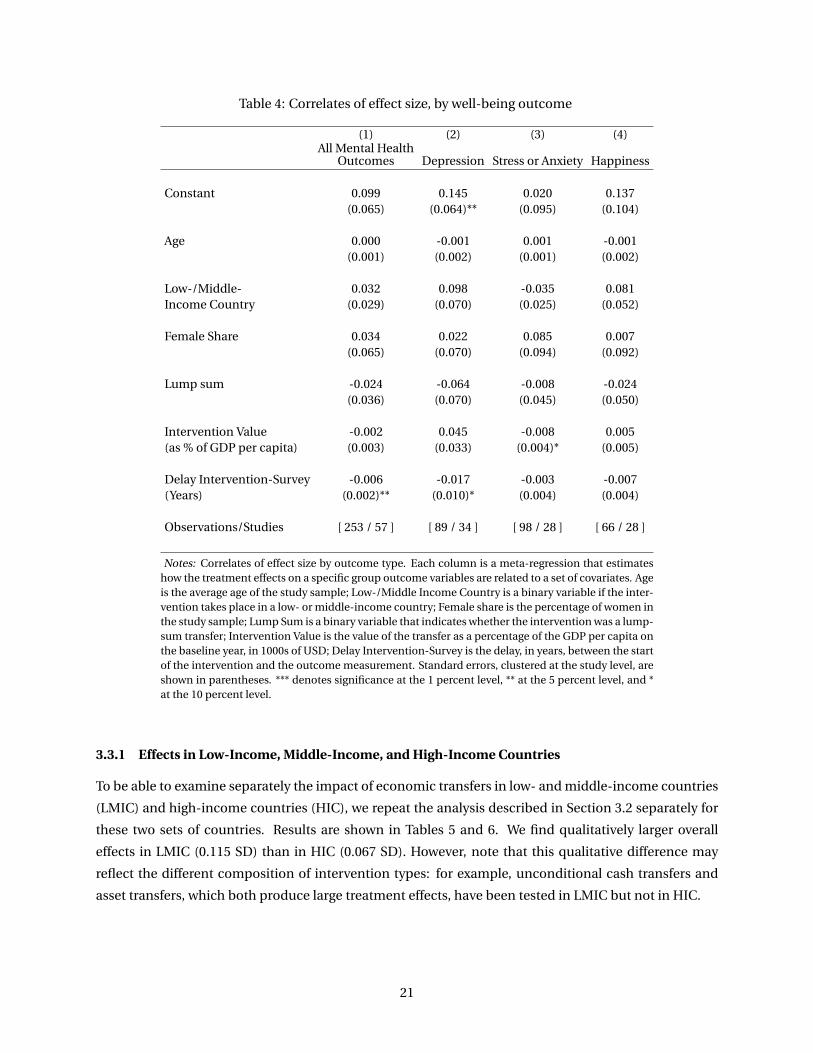
Table 4: Correlates of effect size, by well-being outcome

(1) (2) (3) (4)All Mental Health

Outcomes Depression Stress or Anxiety Happiness

Constant 0.099 0.145 0.020 0.137(0.065) (0.064)** (0.095) (0.104)

Age 0.000 -0.001 0.001 -0.001(0.001) (0.002) (0.001) (0.002)

Low-/Middle- 0.032 0.098 -0.035 0.081Income Country (0.029) (0.070) (0.025) (0.052)

Female Share 0.034 0.022 0.085 0.007(0.065) (0.070) (0.094) (0.092)

Lump sum -0.024 -0.064 -0.008 -0.024(0.036) (0.070) (0.045) (0.050)

Intervention Value -0.002 0.045 -0.008 0.005(as % of GDP per capita) (0.003) (0.033) (0.004)* (0.005)

Delay Intervention-Survey -0.006 -0.017 -0.003 -0.007(Years) (0.002)** (0.010)* (0.004) (0.004)

Observations/Studies [ 253 / 57 ] [ 89 / 34 ] [ 98 / 28 ] [ 66 / 28 ]

Notes: Correlates of effect size by outcome type. Each column is a meta-regression that estimateshow the treatment effects on a specific group outcome variables are related to a set of covariates. Ageis the average age of the study sample; Low-/Middle Income Country is a binary variable if the inter-vention takes place in a low- or middle-income country; Female share is the percentage of women inthe study sample; Lump Sum is a binary variable that indicates whether the intervention was a lump-sum transfer; Intervention Value is the value of the transfer as a percentage of the GDP per capita onthe baseline year, in 1000s of USD; Delay Intervention-Survey is the delay, in years, between the startof the intervention and the outcome measurement. Standard errors, clustered at the study level, areshown in parentheses. *** denotes significance at the 1 percent level, ** at the 5 percent level, and *at the 10 percent level.

3.3.1 Effects in Low-Income, Middle-Income, and High-Income Countries

To be able to examine separately the impact of economic transfers in low- and middle-income countries

(LMIC) and high-income countries (HIC), we repeat the analysis described in Section 3.2 separately for

these two sets of countries. Results are shown in Tables 5 and 6. We find qualitatively larger overall

effects in LMIC (0.115 SD) than in HIC (0.067 SD). However, note that this qualitative difference may

reflect the different composition of intervention types: for example, unconditional cash transfers and

asset transfers, which both produce large treatment effects, have been tested in LMIC but not in HIC.

21

Table 5: Meta-analytic effects: Studies in Low- and Middle-Income Countries

(1) (2) (3) (4)All Mental Health

Outcomes Depression Stress or Anxiety Happiness

All Interventions 0.115 0.136 0.058 0.155(0.018)*** (0.028)*** (0.017)** (0.024)***[ 167 / 39 ] [ 59 / 25 ] [ 56 / 15 ] [ 52 / 20 ]

Unconditional Cash Transfer 0.150 0.163 0.081 0.180(0.023)*** (0.039)*** (0.024)** (0.033)***[ 82 / 27 ] [ 39 / 17 ] [ 18 / 10 ] [ 25 / 13 ]

Conditional Cash Transfer 0.043 0.032 0.045 0.106(0.010)** (0.012) (0.005)* (0.060)*[ 14 / 5 ] [ 7 / 3 ] [ 6 / 2 ] [ 1 / 1 ]

Housing Voucher 0.078 — -0.039 0.196(0.115) (0.036) (0.036)***[ 2 / 1 ] [ 0 / 0 ] [ 1 / 1 ] [ 1 / 1 ]

Poverty Graduation Program 0.079 0.115 0.047 0.124(0.028) (0.005)** (0.027) (0.040)

[ 51 / 3 ] [ 6 / 2 ] [ 28 / 2 ] [ 17 / 2 ]

Lottery Win 1.299 — — 1.299(0.632)** (0.632)**[ 1 / 1 ] [ 0 / 0 ] [ 0 / 0 ] [ 1 / 1 ]

Asset Transfer 0.158 0.137 0.156 0.181(0.048)* (0.057) (0.227) (0.044)[ 12 / 3 ] [ 6 / 3 ] [ 1 / 1 ] [ 5 / 2 ]

Health Insurance Provision 0.121 0.080 0.231 0.028(0.055)** (0.100) (0.067)*** (0.067)[ 5 / 1 ] [ 1 / 1 ] [ 2 / 1 ] [ 2 / 1 ]

Notes: Meta-analytic estimates for the effect of transfers on well-being in low- and middle-incomecountries. This table reproduces Table 2, except that it only includes studies in low- and middle-incomecountries. All other characteristics are as in Table 2.

22

Table 6: Meta-analytic effects: Studies in High-Income Countries

(1) (2) (3) (4)All Mental Health

Outcomes Depression Stress or Anxiety Happiness

All Interventions 0.067 0.099 0.051 0.043(0.005)*** (0.008)** (0.009)** (0.015)**[ 86 / 18 ] [ 30 / 9 ] [ 42 / 13 ] [ 14 / 8 ]

Unconditional Cash Transfer — — — —

[ 0 / 0 ] [ 0 / 0 ] [ 0 / 0 ] [ 0 / 0 ]

Conditional Cash Transfer 0.038 -0.052 0.129 —(0.090) (0.088) (0.088)[ 2 / 1 ] [ 1 / 1 ] [ 1 / 1 ] [ 0 / 0 ]

Housing Voucher 0.069 0.104 0.044 0.057(0.001)** (0.001)** (0.000)** (0.018)**[ 64 / 10 ] [ 25 / 6 ] [ 33 / 9 ] [ 6 / 2 ]

Poverty Graduation Program — — — —

[ 0 / 0 ] [ 0 / 0 ] [ 0 / 0 ] [ 0 / 0 ]

Lottery Win 0.046 — 0.082 0.020(0.020)* (0.022)* (0.009)[ 14 / 5 ] [ 0 / 0 ] [ 8 / 3 ] [ 6 / 4 ]

Asset Transfer — — — —

[ 0 / 0 ] [ 0 / 0 ] [ 0 / 0 ] [ 0 / 0 ]

Health Insurance Provision 0.080 0.081 — 0.100(0.028)** (0.040)** (0.036)**[ 6 / 2 ] [ 4 / 2 ] [ 0 / 0 ] [ 2 / 2 ]

Notes: Meta-analytic estimates for the effect of transfers on well-being in high-income countries. Thistable reproduces Table 2, except that it only includes studies in low- and middle-income countries. Allother characteristics are as in Table 2.

23

3.4 Publication Bias

Recent years have highlighted the possibility of publication bias, i.e. selective publication of “positive”,

surprising, and statistically significant results Andrews and Kasy 2019. To assess to what extent our re-

sults may be affected by such selective publication practices, we adjust our meta-analytic effect size

estimates using three methods: Vevea and Hedges (1995); the P-uniform* method proposed by Aert and

Assen (2018); and Andrews and Kasy (2019) (see Appendix A2 for more information on these methods).

Tables 7 and 8 show the meta-analytic effect size estimates produced by each of these approaches,

by intervention type and well-being outcome, respectively. The first column shows the “naïve” estimates

for comparison. We find little evidence of publication bias; the corrected meta-analytic effect size esti-

mates are numerically close to the overall results. In addition, only a small share of the corrected point

estimates are numerically smaller than the naïve estimates.

The lack of evidence for publication bias may be due to the fact that most of these papers come from

field studies, which tend to publish their results regardless of the outcome. In addition, the well-being

outcomes we analyze here are often not the primary outcomes of interest in the original studies, and

thus may be less affected by publication bias.

24

Table 7: Meta-analytic effects adjusted for publication bias, by intervention type

(1) (2) (3) (4)Naïve

Estimation P-uniform∗ Andrews & Kasy Veva & Hedges

All Interventions 0.100 0.112 0.100 0.138(0.013)*** (0.031)*** (0.010)*** (0.023)***

Unconditional Cash Transfer 0.150 0.192 0.161 0.227(0.025)*** (0.064)** (0.022)*** —

Conditional Cash Transfer 0.043 0.068 0.048 0.092(0.009)** (0.133) (0.019)** (0.064)

Housing Voucher 0.070 0.091 0.037 0.119(0.018)** (0.069)* (0.010)*** (0.027)***

Poverty Graduation Program 0.079 0.091 0.084 0.116(0.028) (0.057)* (0.017)*** —

Lottery Win 0.073 0.038 0.009 0.051(0.029)* (0.074) (0.004)** (0.019)**

Asset Transfer 0.158 0.213 0.201 0.271(0.048)* (0.179) (0.053)*** —

Health Insurance Provision 0.093 0.113 0.057 0.145(0.023)* (0.126) (0.019)** (0.403)

Notes: Meta-analytic effect size estimates adjusted for publication bias, by intervention type. Col-umn 1 reproduces the results from the “naïve” analysis without adjustment. Columns 2–4 showadjusted results using the P-uniform* method; the Andrews & Kasy method; and and the Vevea &Hedges method. The different rows report results for different intervention types. Standard errors,clustered at the study level, are shown in parentheses. *** denotes significance at the 1 percent level,** at the 5 percent level, and * at the 10 percent level.

25

Table 8: Meta-analytic effects adjusted for publication bias, by well-being outcome

(1) (2) (3) (4)Naïve

Estimation P-uniform∗ Andrews & Kasy Vevea & Hedges

All Interventions 0.100 0.112 0.100 0.138(0.013)*** (0.031)*** (0.010)*** (0.023)***

Depression 0.126 0.148 0.136 0.173(0.022)*** (0.060)** (0.020)*** (0.062)**

Stress or Anxiety 0.055 0.068 0.052 0.091(0.010)*** (0.047)* (0.012)*** —

Happiness 0.131 0.152 0.116 0.237(0.019)*** (0.060)** (0.015)*** (0.061)***

Notes: Meta-analytic effect size estimates adjusted for publication bias, by well-beingoutcome. Column 1 reproduces the results from the “naïve” analysis without adjust-ment. Columns 2–4 show adjusted results using the P-uniform* method; the Andrews &Kasy method; and and the Vevea & Hedges method. The different rows report results fordifferent well-being outcomes. Standard errors, clustered at the study level, are shownin parentheses. *** denotes significance at the 1 percent level, ** at the 5 percent level,and * at the 10 percent level.

26

4. Discussion

In this systematic review and meta-analysis, we have summarized the evidence on the effect of economic

transfers on measures of mental health and subjective well-being. We generally find positive effects of

transfers, with an improvement especially in depression, happiness, and life satisfaction. These im-

provements are most robustly documented for unconditional cash transfers (UCTs). Effects decay over

time, but do not differ much depending on the gender of the recipient and the transfer amount.

Together, these results suggest that economic transfers are effective in improving mental health and

subjective well-being, lending support to the “social causation” hypothesis familiar to public health re-

searchers.

While the present study is hopefully a helpful step in better understanding the well-being effects of

economic interventions, it has a number of limitations. First, the overall number of studies is not large,

and especially for individual intervention types and outcome variables, many cells only contain a small

number of studies. This fact raises concerns about external validity, because the inferences drawn for

the particular combination of intervention type and outcome are confounded with the characteristics of

the specific studies, including location, sample, intervention value, and delay between intervention and

outcome measurement. Secondly and relatedly, there is substantial heterogeneity in the effect sizes we

observe, deepening the concerns about individual combinations of interventions and outcomes being

driven by study-specific characteristics, and also weakening the case for summarizing these findings

using meta-analysis. Table A7 shows an overall heterogeneity estimate of I 2 = 93.1%, which is high.15

In addition, the measure fluctuates between 0 and 97% for different intervention types and well-being

outcomes across our sample. At the same time, however, we note that the almost uniformly positive

treatment effects of the interventions we study, despite their heterogeneity, suggests that negative or

zero impacts are unlikely.16.

Together, our results suggest that the renewed interest of policy-makers and others in economic

transfer as welfare interventions is supported not only by the economic impact of such interventions,

but also by their effects on mental health and subjective well-being.

15. I 2 describes the percentage of total variation across studies that is due to heterogeneity rather than chance. It is estimated

as I 2 = 100(Q−d f )

Q , where Q is Cochran’s heterogeneity statistic (the weighted sum of squared differences between individualstudy effects and the pooled effect across studies, with the weights being those used in the pooling method), and d f the degreesof freedom (Higgins et al. 2003).

16. Higgins et al. 2003 note that because systematic reviews bring together studies that are methodologically diverse, hetero-geneity is to be expected, and “there seems little point in simply testing for heterogeneity when what matters is the extent towhich it affects the conclusions of the meta-analysis”

27

References

Aert, Robbie Cornelis Maria van, and Marcel A. L. M. van Assen. 2018. Correcting for Publication Bias ina Meta-Analysis with the P-uniform* Method. Preprint. MetaArXiv, October. Accessed July 2, 2021.https://osf.io/zqjr9.

Alzua, Maria Laura, Maria Natalia Cantet, Ana Dammert, and Daminola Olajide. 2020. “Mental HealthEffects of an Old Age Pension: Experimental Evidence for Ekiti State in Nigeria.”

Andersen, Asbjørn, Andreas Kotsadam, and Vincent Somville. 2021. “Material resources and well-being— Evidence from an Ethiopian housing lottery.” SSRN Electronic Journal, ISSN: 1556-5068, accessedJuly 20, 2021. https://www.ssrn.com/abstract=3834930.

Andrews, Isaiah, and Maximilian Kasy. 2019. “Identification of and Correction for Publication Bias.”American Economic Review 109, no. 8 (August): 2766–2794. ISSN: 0002-8282, accessed July 11, 2021.https://pubs.aeaweb.org/doi/10.1257/aer.20180310.

Angeles, Gustavo, Jacobus de Hoop, Sudhanshu Handa, Kelly Kilburn, Annamaria Milazzo, and Am-ber Peterman. 2019. “Government of Malawi’s unconditional cash transfer improves youth mentalhealth.” Publisher: Elsevier, Social Science & Medicine 225 (C): 108–119. Accessed June 11, 2020.https://ideas.repec.org/a/eee/socmed/v225y2019icp108-119.html.

Assen, Marcel A. L. M. van, Robbie C. M. van Aert, and Jelte M. Wicherts. 2015. “Meta-analysis usingeffect size distributions of only statistically significant studies.” Psychological Methods 20 (3): 293–309. ISSN: 1939-1463, 1082-989X, accessed July 11, 2021. http://doi.apa.org/getdoi.cfm?doi=10.1037/met0000025.

Baicker, Katherine, Sarah L. Taubman, Heidi L. Allen, Mira Bernstein, Jonathan H. Gruber, Joseph P. New-house, Eric C. Schneider, Bill J. Wright, Alan M. Zaslavsky, and Amy N. Finkelstein. 2013. “The Oregonexperiment—effects of Medicaid on clinical outcomes.” New England Journal of Medicine 368 (18):1713–1722.

Baird, Sarah, Jacobus de Hoop, and Berk Özler. 2013. “Income Shocks and Adolescent Mental Health.”Publisher: University of Wisconsin Press, Journal of Human Resources 48 (2): 370–403. AccessedJune 11, 2020. https://ideas.repec.org/a/uwp/jhriss/v48y2013ii1p370-403.html.

Bando, Rosangela, Sebastian Galiani, and Paul Gertler. 2020. “The Effects of Noncontributory Pensionson Material and Subjective Well-Being.” Economic Development and Cultural Change 68 (4).

Banerjee, Abhijit, Esther Duflo, Nathanael Goldberg, Dean Karlan, Robert Osei, William Parienté, JeremyShapiro, Bram Thuysbaert, and Christopher Udry. 2015. “A multifaceted program causes lastingprogress for the very poor: Evidence from six countries.” Science 348, no. 6236 (May): 1260799. ISSN:0036-8075, 1095-9203, accessed May 25, 2016. http://science.sciencemag.org/content/348/6236/1260799.

Banerjee, Ahbijit, Michael Faye, Alan Krueger, Paul Niehaus, and Tavneet Suri. 2020. “Effects of a Univer-sal Basic Income during the pandemic.”

Blattman, Christopher, Nathan Fiala, and Sebastian Martinez. 2011. Employment generation in ruralAfrica: mid-term results from an experimental evaluation of the Youth Opportunities Program inNorthern Uganda. World Bank.

28

Blattman, Christopher, Nathan Fiala, and Sebastian Martinez. 2014. “Generating skilled employment indeveloping countries: Experimental evidence from Uganda.” Quarterly Journal of Economics 129(2): 697–752.

. 2019. The long term impacts of grants on poverty: 9-year evidence from Uganda’s Youth Op-portunities Program. Technical report 802. Publication Title: Ruhr Economic Papers. RWI - Leibniz-Institut für Wirtschaftsforschung, Ruhr-University Bochum, TU Dortmund University, University ofDuisburg-Essen. Accessed September 25, 2020. https://ideas.repec.org/p/zbw/rwirep/802.html.

Blattman, Christopher, Julian C. Jamison, and Margaret Sheridan. 2017. “Reducing Crime and Violence:Experimental Evidence from Cognitive Behavioral Therapy in Liberia.” American Economic Review107, no. 4 (April): 1165–1206. ISSN: 0002-8282, accessed November 4, 2017. https://www.aeaweb.org/articles?id=10.1257/aer.20150503.

Borenstein, Michael, Larry V. Hedges, Julian P.T. Higgins, and Hannah R. Rothstein. 2010. “A basic intro-duction to fixed-effect and random-effects models for meta-analysis.” Research Synthesis Methods1, no. 2 (April): 97–111. ISSN: 17592879, accessed July 2, 2021. http://doi.wiley.com/10.1002/jrsm.12.

Bossuroy, Thomas, Markus Goldstein, Dean Karlan, Harounan Kazianga, William Parienté, Patrick Pre-mand, Catherine Thomas, Christopher Udry, Julia Vaillant, and Kelsey Wright. 2021. Pathways out ofExtreme Poverty: Tackling Psychosocial and Capital Constraints with a Multi-Faceted Social Protec-tion Program in Niger. Policy Research Working Papers. The World Bank, March. Accessed July 20,2021. http://elibrary.worldbank.org/doi/book/10.1596/1813-9450-9562.

Bromet, Evelyn, Laura Helena Andrade, Irving Hwang, Nancy A Sampson, Jordi Alonso, Giovanni de Giro-lamo, Ron de Graaf, et al. 2011. “Cross-national epidemiology of DSM-IV major depressive episode.”BMC Medicine 9, no. 1 (December): 90. ISSN: 1741-7015, accessed July 1, 2021. http://bmcmedicine.biomedcentral.com/articles/10.1186/1741-7015-9-90.

Burger, Martijn J., Martijn Hendriks, Emma Pleeging, and Jan C. van Ours. 2020. “The joy of lottery play:evidence from a field experiment.” Experimental Economics, 1–22.

Edmonds, Eric, and Caroline Theoharides. 2020. “The short term impact of a productive asset transferin families with child labor: Experimental evidence from the philippines.” Journal of DevelopmentEconomics, 102486.

Egger, Dennis, Johannes Haushofer, Edward Miguel, Paul Niehaus, and Michael W. Walker. 2019. Generalequilibrium effects of cash transfers: experimental evidence from Kenya. Technical report. NationalBureau of Economic Research.

Fauth, Rebecca C., Tama Leventhal, and Jeanne Brooks-Gunn. 2004. “Short-term effects of moving frompublic housing in poor to middle-class neighborhoods on low-income, minority adults’ outcomes.”Publisher: Elsevier, Social Science & Medicine 59 (11): 2271–2284. Accessed August 7, 2020. https://ideas.repec.org/a/eee/socmed/v59y2004i11p2271-2284.html.

Fernald, Lia C.H., and Melissa Hidrobo. 2011. “Effect of Ecuador’s cash transfer program (Bono de De-sarrollo Humano) on child development in infants and toddlers: A randomized effectiveness trial.”Social Science & Medicine 72, no. 9 (May): 1437–1446. ISSN: 02779536, accessed June 30, 2021. https://linkinghub.elsevier.com/retrieve/pii/S0277953611001481.

Ferrah, Prepared Samih, and Eric Mvukiyehe. n.d. “Enhancing Female Entrepreneurship through CashGrants: Experimental Evidence from Rural Tunisia,” 52.

29

Finkelstein, Amy, Sarah Taubman, Bill Wright, Mira Bernstein, Jonathan Gruber, Joseph P. Newhouse,Heidi Allen, and Katherine Baicker. 2012. “The Oregon Health Insurance Experiment: Evidence fromthe First Year.” Publisher: Oxford University Press, The Quarterly Journal of Economics 127 (3): 1057–1106. Accessed June 11, 2020. https://ideas.repec.org/a/oup/qjecon/v127y2012i3p1057-1106.html.

Gardner, Jonathan, and Andrew Oswald. 2001. “Does money buy happiness? A longitudinal study usingdata on windfalls.” Manuscript submitted for publication.

Gardner, Jonathan, and Andrew J. Oswald. 2007. “Money and mental wellbeing: A longitudinal study ofmedium-sized lottery wins.” Place: Netherlands Publisher: Elsevier BV, Elsevier, Elsevier Sequoia SA,Journal of Health Economics, Journal of Health Economics, 26 (1): 49–60. ISSN: 0167-6296, accessedJune 29, 2020. http://econpapers.repec.org/article/eeejhecon/v_3a26_3ay_3a2007_3ai_3a1_3ap_3a49-60.htm.

Glass, Nancy, Nancy A. Perrin, Anjalee Kohli, Jacquelyn Campbell, and Mitima Mpanano Remy. 2017.“Randomised controlled trial of a livestock productive asset transfer programme to improve eco-nomic and health outcomes and reduce intimate partner violence in a postconflict setting.” BMJglobal health 2 (1).

Green, E. P., C. Blattman, J. Jamison, and J. Annan. 2016. “Does Poverty Alleviation Decrease DepressionSymptoms in Post-Conflict Settings?: A Cluster-Randomized Trial of Microenterprise Assistance inNorthern Uganda.” Publisher: Cambridge University Press, Global Mental Health, ISSN: 2054-4251.

Haushofer, Johannes, Matthieu Chemin, Chaning Jang, and Justin Abraham. 2020. “Economic and psy-chological effects of health insurance and cash transfers: Evidence from a randomized experimentin Kenya.” Publisher: Elsevier, Journal of Development Economics 144 (C). Accessed June 11, 2020.https://ideas.repec.org/a/eee/deveco/v144y2020ics0304387818310289.html.

Haushofer, Johannes, Robert Mudida, and Jeremy Shapiro. 2019. “The Comparative Impact of Cash Trans-fers and Psychotherapy on Psychological and Economic Well-being.”

. 2020. “The Comparative Impact of Cash Transfers and Psychotherapy on Psychological and Eco-nomic Well-being.”

Haushofer, Johannes, and Jeremy Shapiro. 2016. “The Short-term Impact of Unconditional Cash Trans-fers to the Poor: ExperimentalEvidence from Kenya.” Publisher: Oxford University Press, The Quar-terly Journal of Economics 131 (4): 1973–2042. Accessed June 11, 2020. https://ideas.repec.org/a/oup/qjecon/v131y2016i4p1973-2042..html.

. 2018. “The long-term impact of unconditional cash transfers: Experimental evidence from Kenya,”64.

Heath, Rachel, Melissa Hidrobo, and Shalini Roy. 2020. “Cash transfers, polygamy, and intimate partnerviolence: Experimental evidence from Mali.” Journal of Development Economics 143:102410.

Higgins, Julian P. T., James Thomas, Jacqueline Chandler, Miranda Cumpston, Tianjing Li, Matthew J.Page, and Vivian A. Welch. 2019. Cochrane Handbook for Systematic Reviews of Interventions. Google-Books-ID: cTqyDwAAQBAJ. John Wiley & Sons, September. ISBN: 978-1-119-53661-1.

Higgins, Julian P. T., Simon G. Thompson, Jonathan J. Deeks, and Douglas G. Altman. 2003. “Measuringinconsistency in meta-analyses.” BMJ (Clinical research ed.) 327, no. 7414 (September): 557–560.ISSN: 1756-1833.

30

Hjelm, Lisa, Sudhanshu Handa, Jacobus de Hoop, Tia Palermo, C. G. P. Zambia, and MCP EvaluationTeams. 2017. “Poverty and perceived stress: Evidence from two unconditional cash transfer pro-grams in Zambia.” Social Science & Medicine 177:110–117.

Ismayilova, Leyla, Leyla Karimli, Jo Sanson, Eleni Gaveras, Rachel Nanema, Alexice Tô-Camier, and JoshChaffin. 2018. “Improving mental health among ultra-poor children: Two-year outcomes of a cluster-randomized trial in Burkina Faso.” Publisher: Elsevier, Social Science & Medicine 208 (C): 180–189.Accessed June 11, 2020. https://ideas.repec.org/a/eee/socmed/v208y2018icp180-189.html.

Katz, Lawrence F., Jeffrey R. Kling, and Jeffrey B. Liebman. 2001. “Moving to Opportunity in Boston: EarlyResults of a Randomized Mobility Experiment.” Publisher: Oxford University Press, The QuarterlyJournal of Economics 116 (2): 607–654. Accessed August 12, 2020. https://ideas.repec.org/a/oup/qjecon/v116y2001i2p607-654..html.

Kessler, Ronald C., Greg J. Duncan, Lisa A. Gennetian, Lawrence F. Katz, Jeffrey R. Kling, Nancy A. Samp-son, Lisa Sanbonmatsu, Alan M. Zaslavsky, and Jens Ludwig. 2014. “Associations of housing mobilityinterventions for children in high-poverty neighborhoods with subsequent mental disorders duringadolescence.” Jama 311 (9): 937–947.

Kilburn, Kelly, Sudhanshu Handa, Gustavo Angeles, Maxton Tsoka, and Peter Mvula. 2018. “Paying forHappiness: Experimental Results from a Large Cash Transfer Program in Malawi.” Publisher: JohnWiley & Sons, Ltd. Journal of Policy Analysis and Management 37 (2): 331–356. Accessed August 2,2020. https://ideas.repec.org/a/wly/jpamgt/v37y2018i2p331-356.html.

Kilburn, Kelly, James P. Hughes, Catherine MacPhail, Ryan G. Wagner, F. Xavier Gómez-Olivé, KathleenKahn, and Audrey Pettifor. 2019. “Cash transfers, young women’s economic well-being, and HIV risk:evidence from HPTN 068.” AIDS and Behavior 23 (5): 1178–1194.

Kim, Seonghoon, and Andrew J. Oswald. 2021. “Happy Lottery Winners and Lottery-Ticket Bias.” Reviewof Income and Wealth 67, no. 2 (June): 317–333. ISSN: 0034-6586, 1475-4991, accessed June 30, 2021.https://onlinelibrary.wiley.com/doi/10.1111/roiw.12469.

Kling, Jeffrey R., Jeffrey B. Liebman, and Lawrence F. Katz. 2007. “Experimental Analysis of NeighborhoodEffects.” Publisher: Econometric Society, Econometrica 75 (1): 83–119. Accessed August 12, 2020.https://ideas.repec.org/a/ecm/emetrp/v75y2007i1p83-119.html.

Kuhn, Peter, Peter Kooreman, Adriaan Soetevent, and Arie Kapteyn. 2011. “The effects of lottery prizeson winners and their neighbors: Evidence from the Dutch postcode lottery.” American EconomicReview 101 (5): 2226–47.

Lau, Joseph, John P A Ioannidis, Norma Terrin, Christopher H Schmid, and Ingram Olkin. 2006. “The caseof the misleading funnel plot.” BMJ 333, no. 7568 (September): 597–600. ISSN: 0959-8138, 1468-5833,accessed July 11, 2021. https://www.bmj.com/lookup/doi/10.1136/bmj.333.7568.597.

Leventhal, T., and J. Brooks-Gunn. 2003. “Moving to Oppurtunity: An Experimental Study of Neighbor-hood Effects on Mental Health.” Publisher: American Public Health Association, American Journalof Public Health 93 (9): 1576–1582. Accessed June 11, 2020. https://ideas.repec.org/a/aph/ajpbhl/20039391576-1582_8.html.

31

Leventhal, Tama, and Véronique Dupéré. 2011. “Moving to Opportunity: Does long-term exposure to’low-poverty’ neighborhoods make a difference for adolescents?” Publisher: Elsevier, Social Science& Medicine 73 (5): 737–743. Accessed June 11, 2020. https : / / ideas . repec . org / a / eee / socmed /v73y2011i5p737-743.html.

Lindqvist, Erik, Robert Östling, and David Cesarini. 2020. “Long-Run Effects of Lottery Wealth on Psy-chological Well-Being.” The Review of Economic Studies, accessed September 6, 2020. https : / /academic.oup.com/restud/advance-article/doi/10.1093/restud/rdaa006/5734654.

Ludwig, Jens, Greg J. Duncan, Lisa A. Gennetian, Lawrence F. Katz, Ronald C. Kessler, Jeffrey R. Kling,and Lisa Sanbonmatsu. 2013. “Long-Term Neighborhood Effects on Low-Income Families: Evidencefrom Moving to Opportunity.” Publisher: American Economic Association, American Economic Re-view 103 (3): 226–231. Accessed June 11, 2020. https://ideas.repec.org/a/aea/aecrev/v103y2013i3p226-31.html.

Lund, Crick, Alison Breen, Alan J. Flisher, Ritsuko Kakuma, Joanne Corrigall, John A. Joska, Leslie Swartz,and Vikram Patel. 2010. “Poverty and common mental disorders in low and middle income coun-tries: A systematic review.” Social Science & Medicine 71, no. 3 (August): 517–528. ISSN: 02779536,accessed July 1, 2021. https://linkinghub.elsevier.com/retrieve/pii/S0277953610003576.

Lund, Crick, Mary De Silva, Sophie Plagerson, Sara Cooper, Dan Chisholm, Jishnu Das, Martin Knapp,and Vikram Patel. 2011. “Poverty and mental disorders: breaking the cycle in low-income and middle-income countries.” Publisher: Elsevier Ltd, The Lancet 378 (9801): 1502–1514. ISSN: 0140-6736.

Macours, Karen, Norbert Schady, and Renos Vakis. 2012. “Cash Transfers, Behavioral Changes, and Cog-nitive Development in Early Childhood: Evidence from a Randomized Experiment.” American Eco-nomic Journal: Applied Economics 4, no. 2 (April): 247–273. ISSN: 1945-7782, 1945-7790, accessedJune 30, 2021. https://pubs.aeaweb.org/doi/10.1257/app.4.2.247.

McGuire, Joel, Caspar Kaiser, and Anders Bach-Mortensen. 2020. The impact of cash transfers on sub-jective well-being and mental health in low- and middle- income countries: A systematic review andmeta-analysis. Preprint. SocArXiv, November. Accessed September 14, 2021. https://osf.io/ydr54.

McIntosh, Craig, and Andrew Zeitlin. 2020. “Using Household Grants to Benchmark the Cost Effective-ness of a USAID Workforce Readiness Program.” ArXiv: 2009.01749, arXiv:2009.01749 [econ, q-fin](September). Accessed September 25, 2020. http://arxiv.org/abs/2009.01749.

Molotsky, Adria, and Sudhanshu Handa. 2021. “The Psychology of Poverty: Evidence from the Field.”Journal of African Economies 30, no. 3 (June): 207–224. ISSN: 0963-8024, 1464-3723, accessed June 30,2021. https://academic.oup.com/jae/article/30/3/207/6015888.

Morris, Pamela A., J. Lawrence Aber, Sharon Wolf, and Juliette Berg. 2017. “Impacts of family rewardson adolescents’ mental health and problem behavior: Understanding the full range of effects of aconditional cash transfer program.” Prevention Science 18 (3): 326–336.

Muller, Angelika, Utz Johann Pape, and Laura R. Ralston. 2019. Broken Promises : Evaluating an Incom-plete Cash Transfer Program. Technical report 9016. Publication Title: Policy Research Working Pa-per Series. The World Bank, September. Accessed June 11, 2020. https://ideas.repec.org/p/wbk/wbrwps/9016.html.

32

Natali, Luisa, Sudhanshu Handa, Amber Peterman, David Seidenfeld, and Gelson Tembo. 2018. “Doesmoney buy happiness? Evidence from an unconditional cash transfer in Zambia.” SSM-populationhealth 4:225–235.

Nguyen, Quynh C., Nicole M. Schmidt, M. Maria Glymour, David H. Rehkopf, and Theresa L. Osypuk.2013. “Were the mental health benefits of a housing mobility intervention larger for adolescents inhigher socioeconomic status families?” Health & place 23:79–88.

Ohrnberger, Julius, Eleonora Fichera, Matt Sutton, and Laura Anselmi. 2020. “The worse the better?Quantile treatment effects of a conditional cash transfer programme on mental health.” Health Pol-icy and Planning.

Osypuk, Theresa L., Nicole M. Schmidt, Lisa M. Bates, Eric J. Tchetgen-Tchetgen, Felton J. Earls, andM. Maria Glymour. 2012. “Gender and crime victimization modify neighborhood effects on adoles-cent mental health.” Pediatrics 130 (3): 472–481.

Paxson, Christina, and Norbert Schady. 2010. “Does money matter? The effects of cash transfers on childdevelopment in rural Ecuador.” Economic development and cultural change 59 (1): 187–229.

Quattrochi, John, Ghislain Bisimwa, Peter Van der Windt, and Maarten Voors. 2020. “Effect of an Eco-nomic Transfer Program on Mental Health of Displaced Persons and Host Populations in DemocraticRepublic of Congo: A Randomised Controlled Trial.” SSRN Electronic Journal, ISSN: 1556-5068, ac-cessed June 30, 2021. https://www.ssrn.com/abstract=3706054.

Ridley, Matthew, Gautam Rao, Frank Schilbach, and Vikram Patel. 2020. “Poverty, depression, and anx-iety: Causal evidence and mechanisms.” Publisher: American Association for the Advancement ofScience, Science 370, no. 6522 (December): eaay0214. Accessed September 14, 2021. https://www.science.org/doi/10.1126/science.aay0214.

Roy, Shalini, Melissa Hidrobo, John F. Hoddinott, Bastien Koch, and Akhter Ahmed. 2019. Can transfersand behavior change communication reduce intimate partner violence four years post-program?Experimental evidence from Bangladesh: technical report 1869. Publication Title: IFPRI discussionpapers. International Food Policy Research Institute (IFPRI). Accessed August 2, 2020. https://ideas.repec.org/p/fpr/ifprid/1869.html.

Sanbonmatsu, Lisa, Lawrence F. Katz, Jens Ludwig, Lisa A. Gennetian, Greg J. Duncan, Ronald C. Kessler,Emma K. Adam, Thomas McDade, and Stacy T. Lindau. 2011. “Moving to opportunity for fair housingdemonstration program: Final impacts evaluation.”

Stein, Daniel, Heather E. Lanthorn, Emma Kimani, and Rico Bergemann. 2020. Cash transfers and COVID-19: Experiences from Kiryandongo refugee settlement, Uganda. Technical report. IDinsight.

Vevea, Jack L., and Larry V. Hedges. 1995. “A general linear model for estimating effect size in the presenceof publication bias.” Psychometrika 60, no. 3 (September): 419–435. ISSN: 0033-3123, 1860-0980, ac-cessed July 11, 2021. http://link.springer.com/10.1007/BF02294384.

33

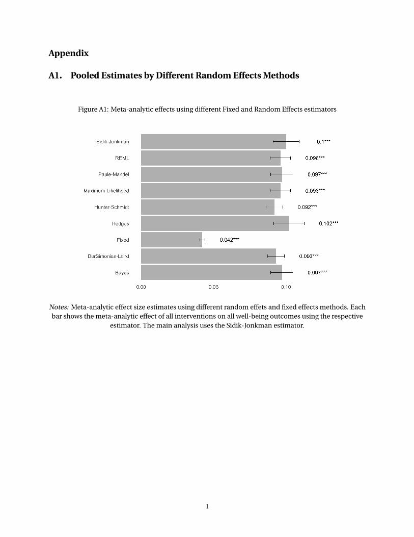
Appendix

A1. Pooled Estimates by Different Random Effects Methods

Figure A1: Meta-analytic effects using different Fixed and Random Effects estimators

Notes: Meta-analytic effect size estimates using different random effets and fixed effects methods. Eachbar shows the meta-analytic effect of all interventions on all well-being outcomes using the respective

estimator. The main analysis uses the Sidik-Jonkman estimator.

1

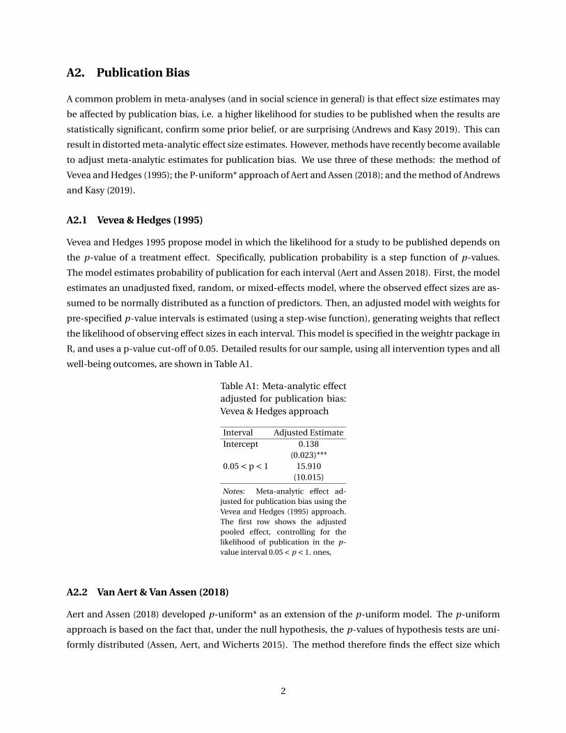
A2. Publication Bias

A common problem in meta-analyses (and in social science in general) is that effect size estimates may

be affected by publication bias, i.e. a higher likelihood for studies to be published when the results are

statistically significant, confirm some prior belief, or are surprising (Andrews and Kasy 2019). This can

result in distorted meta-analytic effect size estimates. However, methods have recently become available

to adjust meta-analytic estimates for publication bias. We use three of these methods: the method of

Vevea and Hedges (1995); the P-uniform* approach of Aert and Assen (2018); and the method of Andrews

and Kasy (2019).

A2.1 Vevea & Hedges (1995)

Vevea and Hedges 1995 propose model in which the likelihood for a study to be published depends on

the p-value of a treatment effect. Specifically, publication probability is a step function of p-values.

The model estimates probability of publication for each interval (Aert and Assen 2018). First, the model

estimates an unadjusted fixed, random, or mixed-effects model, where the observed effect sizes are as-

sumed to be normally distributed as a function of predictors. Then, an adjusted model with weights for

pre-specified p-value intervals is estimated (using a step-wise function), generating weights that reflect

the likelihood of observing effect sizes in each interval. This model is specified in the weightr package in

R, and uses a p-value cut-off of 0.05. Detailed results for our sample, using all intervention types and all

well-being outcomes, are shown in Table A1.

Table A1: Meta-analytic effectadjusted for publication bias:Vevea & Hedges approach

Interval Adjusted EstimateIntercept 0.138

(0.023)***0.05 < p < 1 15.910

(10.015)

Notes: Meta-analytic effect ad-justed for publication bias using theVevea and Hedges (1995) approach.The first row shows the adjustedpooled effect, controlling for thelikelihood of publication in the p-value interval 0.05 < p < 1. ones,

A2.2 Van Aert & Van Assen (2018)

Aert and Assen (2018) developed p-uniform* as an extension of the p-uniform model. The p-uniform

approach is based on the fact that, under the null hypothesis, the p-values of hypothesis tests are uni-

formly distributed (Assen, Aert, and Wicherts 2015). The method therefore finds the effect size which

2

generates a uniform distribution of p-values when it is used as the null hypothesis. The approach mod-

els all studies with statistically significant findings as equally likely to be published and included in the

meta-analysis (Assen, Aert, and Wicherts 2015). The method has three drawbacks: (1) it uses only statis-

tically significant effect sizes; (2) effect size estimates are positively biased when there is between-study

variance in the true effect size; and (3) the approach does not estimate and test for presence of this

between-study variance (Aert and Assen 2018).

The p-uniform* approach addresses these drawbacks. It assumes that the probability of publish-

ing a statistically significant effect size and a non-statistically significant one are constant, but may be

different around a cut-off value (for example, around p = 0.05; Aert and Assen 2018). It uses a maxi-

mum likelihood estimation with truncated densities in between the cut-offs, which allows to implicitly

estimate the weights. This model is specified in the puniform package in R.

Tables A2 and A3 compare the p-uniform and p-uniform* approaches. Each column shows the meta-

analytic treatment effect estimate for a different method available within each of the two approaches. In

Table ??, the different methods to test the uniformity of the p-values are: P (Irwin-Hall), LNP (Fisher),

LN1MINP (transforming p values to 1-P before applying Fisher’s method), and Kolmogorov-Smirnov. In

Table A3, the methods are P (Irwin-Hall), LNP (Fisher), and ML (maximum likelihood estimation of the

effect size and the between-study variance). Using the p-uniform approach, we find very large meta-

analytic effect sizes, that substantially exceed those of the naïve approach. In contrast, the estimates

produced by the p-uniform* approach are very close to those produced by the naïve approach.

Table A2: Meta-analytic effects adjusted for pub-lication bias: P-uniform approach

Estimation P LNP LN1MINP KS

All Interventions 0.396 0.303 0.480 0.396(0.414)* (0.508) (0.330) -

Notes: Meta-analytic effect adjusted for publication biasusing the p-uniform approach. Each column shows themeta-analytic effect size estimate corresponding to a differ-ent method to test uniformity of p-values: P (Irwin-Hall),LNP (Fisher), LN1MINP (transforming p values to 1-P beforeapplying Fisher’s method), and Kolmogorov-Smirnov.

A2.3 Andrews & Kasy

Andrews and Kasy (2019) propose a selection model that corrects the estimates for a known probability

of publication, and this probability can be estimated around specific cut-offs of p-values. It makes the

following distributional and functional form assumptions: publication bias is assumed be to a step func-

tion; the distribution of effect sizes is normal; and effect sizes and sample sizes are independent. While

this latter assumption is common, it has been criticized as unrealistic, given that researchers often use

power calculations to determine sample size (Lau et al. 2006).

3

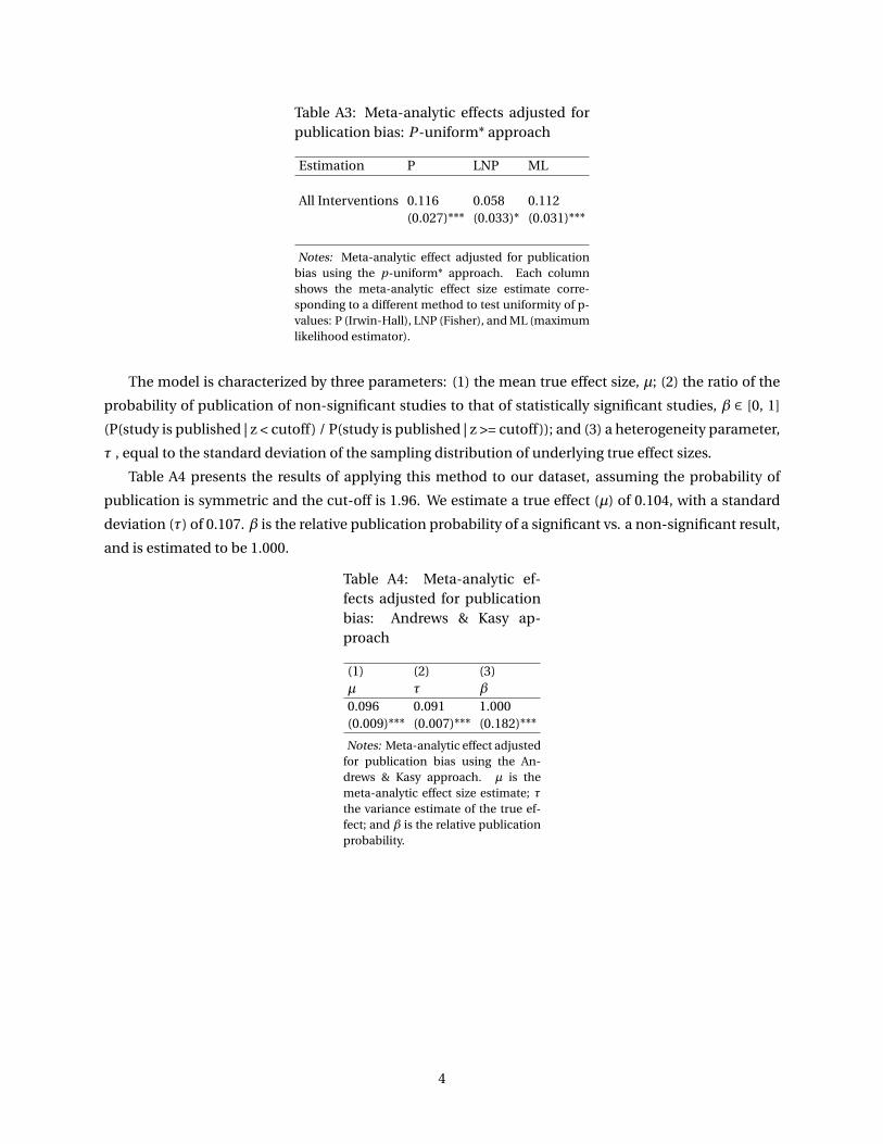
Table A3: Meta-analytic effects adjusted forpublication bias: P-uniform* approach

Estimation P LNP ML

All Interventions 0.116 0.058 0.112(0.027)*** (0.033)* (0.031)***

Notes: Meta-analytic effect adjusted for publicationbias using the p-uniform* approach. Each columnshows the meta-analytic effect size estimate corre-sponding to a different method to test uniformity of p-values: P (Irwin-Hall), LNP (Fisher), and ML (maximumlikelihood estimator).

The model is characterized by three parameters: (1) the mean true effect size, µ; (2) the ratio of the

probability of publication of non-significant studies to that of statistically significant studies, β ∈ [0, 1]

(P(study is published | z < cutoff) / P(study is published | z >= cutoff)); and (3) a heterogeneity parameter,

τ , equal to the standard deviation of the sampling distribution of underlying true effect sizes.

Table A4 presents the results of applying this method to our dataset, assuming the probability of

publication is symmetric and the cut-off is 1.96. We estimate a true effect (µ) of 0.104, with a standard

deviation (τ) of 0.107. β is the relative publication probability of a significant vs. a non-significant result,

and is estimated to be 1.000.

Table A4: Meta-analytic ef-fects adjusted for publicationbias: Andrews & Kasy ap-proach

(1) (2) (3)µ τ β

0.096 0.091 1.000(0.009)*** (0.007)*** (0.182)***

Notes: Meta-analytic effect adjustedfor publication bias using the An-drews & Kasy approach. µ is themeta-analytic effect size estimate; τthe variance estimate of the true ef-fect; and β is the relative publicationprobability.

4

A3. Cash vs. In-kind transfers

Table A5: Meta-analytic effects for cash and in-kind transfers

(1) (2) (3) (4)All Mental Health

Outcomes Depression Stress or Anxiety Happiness

All Interventions 0.100 0.126 0.055 0.131(0.013)*** (0.021)*** (0.010)*** (0.019)***[ 253 / 57 ] [ 89 / 34 ] [ 98 / 28 ] [ 66 / 28 ]

In Cash 0.131 0.138 0.073 0.176(0.020)*** (0.036)** (0.016)** (0.032)***[ 98 / 32 ] [ 47 / 21 ] [ 25 / 12 ] [ 26 / 14 ]

In Kind 0.080 0.111 0.051 0.104(0.012)*** (0.010)*** (0.011)** (0.018)***[ 155 / 26 ] [ 42 / 14 ] [ 73 / 17 ] [ 40 / 15 ]

Notes: Meta-analytic effect size estimates for specific combinations of interventions(rows) and outcomes (columns). The first row shows the impact of any intervention onvarious mental health outcomes, the remaining rows correspond to interventions deliv-ered in-cash or in-kind. Similarly, the first column reports the effect of interventions onany mental health outcome, while the remaining columns focus on specific outcomes.Each cell shows the meta-analytic effect size estimate using random effects with the Sidik-Jonkman estimator. Standard errors, clustered at the study level, are shown in parenthe-ses, and the numbers of effects and studies in brackets. *** denotes significance at the 1percent level, ** at the 5 percent level, and * at the 10 percent level.

5

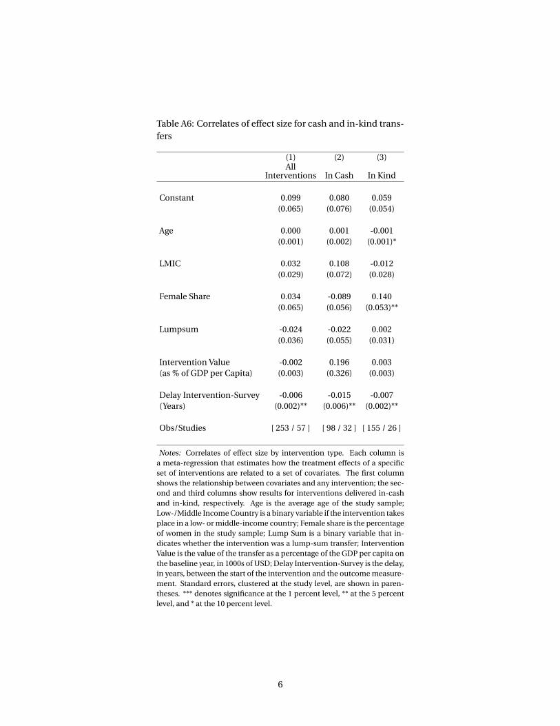
Table A6: Correlates of effect size for cash and in-kind trans-fers

(1) (2) (3)All

Interventions In Cash In Kind

Constant 0.099 0.080 0.059(0.065) (0.076) (0.054)

Age 0.000 0.001 -0.001(0.001) (0.002) (0.001)*

LMIC 0.032 0.108 -0.012(0.029) (0.072) (0.028)

Female Share 0.034 -0.089 0.140(0.065) (0.056) (0.053)**

Lumpsum -0.024 -0.022 0.002(0.036) (0.055) (0.031)

Intervention Value -0.002 0.196 0.003(as % of GDP per Capita) (0.003) (0.326) (0.003)

Delay Intervention-Survey -0.006 -0.015 -0.007(Years) (0.002)** (0.006)** (0.002)**

Obs/Studies [ 253 / 57 ] [ 98 / 32 ] [ 155 / 26 ]

Notes: Correlates of effect size by intervention type. Each column isa meta-regression that estimates how the treatment effects of a specificset of interventions are related to a set of covariates. The first columnshows the relationship between covariates and any intervention; the sec-ond and third columns show results for interventions delivered in-cashand in-kind, respectively. Age is the average age of the study sample;Low-/Middle Income Country is a binary variable if the intervention takesplace in a low- or middle-income country; Female share is the percentageof women in the study sample; Lump Sum is a binary variable that in-dicates whether the intervention was a lump-sum transfer; InterventionValue is the value of the transfer as a percentage of the GDP per capita onthe baseline year, in 1000s of USD; Delay Intervention-Survey is the delay,in years, between the start of the intervention and the outcome measure-ment. Standard errors, clustered at the study level, are shown in paren-theses. *** denotes significance at the 1 percent level, ** at the 5 percentlevel, and * at the 10 percent level.

6

A4. Study Heterogeneity

Table A7: Heterogeneity of Studies: I 2 Statistic

(1) (2) (3) (4)All Mental Health

Outcomes Depression Stress or Anxiety Happiness

All Interventions 93.1 88.3 83.7 96.6[ 240 / 58 ] [ 82 / 33 ] [ 92 / 28 ] [ 66 / 26 ]

Unconditional Cash Transfer 88.5 88.9 61.4 91.4[ 84 / 26 ] [ 38 / 15 ] [ 19 / 10 ] [ 27 / 12 ]

Conditional Cash Transfer 45.1 62.5 29.2 21.3[ 16 / 8 ] [ 5 / 4 ] [ 6 / 3 ] [ 5 / 3 ]

Housing Voucher 77.6 79.5 69.1 23.7[ 63 / 10 ] [ 24 / 6 ] [ 33 / 9 ] [ 6 / 2 ]

Poverty Graduation Program 80.3 0.2 82.8 51.9[ 35 / 2 ] [ 2 / 1 ] [ 20 / 1 ] [ 13 / 1 ]

Lottery Win 98.5 - 94.7 92.1[ 14 / 5 ] - [ 8 / 3 ] [ 6 / 4 ]

Asset Transfer 62.3 60.9 0.6 70.7[ 13 / 4 ] [ 6 / 3 ] [ 2 / 2 ] [ 5 / 2 ]

Health Insurance Provision 80.3 83.3 26.7 15.9[ 11 / 3 ] [ 5 / 3 ] [ 2 / 1 ] [ 4 / 3 ]

Notes: Heterogeneity statistic I 2 for each meta-analytic effects estimation presented in Table 2. TheI 2 estimates the proportion of the variance in study estimates that is due to heterogeneity, as calculatedin Higgins (2003). The standard thresholds according to Higgins et al. 2019 are: 0% to 40%: might not beimportant; 30% to 60%: may represent moderate heterogeneity; 50% to 90%: may represent substantialheterogeneity; 75% to 100%: considerable heterogeneity.

7