1

The Effect of International Remittances on Poverty and

Inequality in Ethiopia

Berhe Mekonnen Beyene†

April, 2011

Abstract

The paper studies the effect of international remittances on poverty and inequality in Ethiopia

using urban household survey collected in 2004. Counterfactual consumption is estimated in the

hypothetical case of no migration and no remittance using information on those households who

don’t receive remittance in a selection corrected estimation framework. Inequality and poverty

values in the hypothetical and actual cases are then compared. Even though only 14% of the

households received remittance, poverty decreased significantly because the remittance receiving

households mainly come from the bottom consumption distribution and the amount they received

is big. The head count ratio fell from 30% to 25% while the poverty gap and the squared poverty

gap ratios respectively decreased from 6.6% to 5.2% and from 2.2% to 1.7%. Inequality

increased but the magnitude is negligible. The Gini coefficient increased from 21.2% to 22.5%.

Key words: remittances, poverty, inequality, Ethiopia

JEL Classification: F-24, I-32, O-15

† University of Oslo, e-mail: b.m.beyene@econ.uio.no. I thank Halvor Mehlum, Kalle Moene

and Jo Thori Lind for comments and suggestions. While carrying out this research I have been

associated with the Centre of Equality, Social Organization, and Performance (ESOP) at the

department of Economics, at the University of Oslo. ESOP is supported by the Research Council

of Norway

2

I. Introduction

International remittances are becoming increasingly important sources of finance for less

developed countries. According to World Bank estimates, the total amount of international

remittances sent to developing countries in 2008 was 325 Billion USD while the foreign direct

investment for the same year was 593 Billion USD. East Asia and the Pacific got the highest

amount with 86 Billion followed by South Asia with 72 Billion while Sub-Saharan-Africa got

the least with 21 Billion. It is worth noting that the World Bank estimate is based on formal

transfers and hence is bound to underestimate the actual size of remittances. In the recent global

financial crisis, despite the common fear that the flow of remittances to developing countries

might fall substantially, it decreased only by 5.5% between 2008 and 2009 to quickly recover in

2010 back to what it was in 2008. In contrast FDI dropped by 40% between 2008 and 2009. In

2008 the total official remittances to Ethiopia was 387 Million USD which was 1.5% of the

annual GDP in that year. Even if the remittance flow to Ethiopia is low its growth is remarkable;

just between 2006 and 2008 it more than doubled (World Bank, 2011).

At macro level, remittances, on top of serving as sources of foreign currency, increase

consumption and investment there by boosting economic growth (Anyanwu and Erhijakpor,

2010). As such, they neutralize (at least partly) the possible human capital loss from migration.

At micro level, remittances improve the welfare of the receiving households by increasing their

income and consumption. There is also evidence that remittance money is invested on small

businesses and education (Edward and Ureta, 2003; Adams, 2003). Further more, remittances

may serve as insurance against income shocks like crop failure (Yang and Choi, 2007). To the

extent that some of the remittance receiving households come from the lower income spectrum,

3

remittances can also decrease poverty and inequality (Acosta et al, 2008). But, if remittances go

mainly to the high income group the impact on poverty will be small or zero while inequality

will be worsened (Adams, 1989; Rodriguez, 1998).1

Studying the effect of remittances on poverty and inequality has a paramount importance in

understanding the overall effect of remittances and in informing policies related with migration

and remittances. To the extent that poverty reduction is a top priority to many developing

countries and international organizations, it is important to know how poverty is affected by

remittances. Also important is the knowledge about the impact of remittances on inequality.

Inequality will decrease if remittances are skewed in favor of the low income households. While

lower inequality is good by itself, it also means more people will be less constrained financially

and will be investing on physical and human capital which will promote economic growth. High

inequality on the contrary lowers investment there by slowing growth (Furman and Stiglitz,

1998; Easterly, 2006). It also makes a pro-poor growth less successful as the poor will be less

likely to benefit from growth (Ravallion, 2001; 2005). Coupled with some socio-cultural factors

it may also trigger polarization and conflict which in turn will destroy economic activities and

institutions (Cramer, 2003). In the long run, high inequality may lead to the subversion of legal,

political, and regulatory institutions by the rich especially in countries where institutions are

weak (Glaeser et al, 2003). Thus, if remittances aggravate inequality, there will be various

negative consequences which dampen, if not totally reverse, the positive effects.

There have been some studies on the effect of remittances on poverty and inequality and the

result so far is not conclusive and varies from study to study. Most of the studies are at micro

level using household survey and concentrate in Latin American countries where remittances are

1 Remittances may also create a moral hazard problem of increasing unemployment or lowering work efforts

(Acosta, 2006; Grigorian and Malkonyan, 2008).

4

very common. There are few studies in African also. There is no study in Ethiopia that deals with

the effect of remittances on poverty and inequality.

This paper studies the effect of remittances on poverty and inequality in Ethiopia using

counterfactual estimation method. First, consumption function is estimated from observations on

households who do not receive remittances and the result is used to construct counterfactual

consumption for remittance receiving households in the hypothetical case of no migration and no

remittances. To account for possible selection in to migration and remittance, the two stage

Hickman selection method is employed. The poverty and inequality measures in the

counterfactual case are then compared with the poverty and inequality measures of the actual

one.

The rest of the paper is organized as follows. Section two reviews existing evidence on the

impact of remittances on poverty and inequality. Section three presents the empirical strategies

employed. In section four, overview of remittance in Ethiopia, data, variable description and

summary statistics are given. The regression results are reported in section five while section six

presents the effect on poverty and inequality. The last section concludes.

II. Summary of Existing Evidence

One of the most obvious and direct effects of remittances is change in the distribution of income

in the receiving country which in turn may affect poverty and inequality depending on who

receives them. While the poor will have more demand to send some member(s) abroad as a

mechanism of improving their welfare the fact that migration is usually expensive and risky also

means that they are less likely to realize it in the absence of well functioning insurance and credit

markets. Thus, to the extent that it is not known a priory who benefit from remittance, the effect

on poverty and inequality is not clear.

5

In the migration literature, it is well established that in areas where migration is on its early

stage, migration is expensive and risky and hence it is only the better-off households who will

afford to send a migrant member abroad and benefit from remittances. As a consequence,

inequality will be aggravated while the effect on poverty will be none or very small. But, as

migration increases through time, information about migration will be easily available which will

make migration less costly and less risky. Past migrants also help new migrants to find a job and

settle in easily. This will enable more and more households to send their members abroad and

benefit from remittances. In the limit, even the very poor will afford to send migrant members

abroad and benefit from remittances. At this stage, migration will be inequality and poverty

reducing (Massey, 1990; Massey and Espinosa, 1997; Mckenzie and Rapoport, 2007). Shen et al

(2010) shows similar result but without migration networks. They argued that initially the cost of

migration is high for the poor and it is mainly the rich who will benefit from migration. As a

result, inequality will be worsened. But, as time goes by, the poor will accumulate wealth

through intergenerational transfers and become less constrained financially. Hence, they will

start to send bigger share of their labor and benefit more from migration. Thus, in the long run

inequality will be reduced. By the same token it could be argued that remittances are more

equalizing (less unequalizing) in areas where there is longer migration history. In the same vein,

Gonzalez-Konig and Wodon (2005) reason that migration is more unequalizing (or less

equalizing) in low income areas than in high income areas because in low income areas only the

rich afford migration and hence benefit from remittances while in high income areas households

in the middle and bottom income distribution may also benefit from remittances.

Interest on the effect of remittances on the receiving country has increased recently and there

have particularly been a number of studies on the impact of remittances on poverty and

6

inequality. Though there are some evidences that remittances decrease poverty and increase

inequality, the result in general is mixed and varies a lot. Most of the studies are country specific

and concentrate in Latin America. There are also few studies in Africa. Cross-country studies are

also emerging recently.

Gustufsson and Mekonnen (1993) studied the effect of remittances on poverty using data

from Lesotho. They treated remittances as exogenous additions to income and compared poverty

measures in the actual case with the counterfactual one where remittances are assumed to be zero

and the migrants are back home with no income. The result shows that remittances decreased

poverty significantly. The effect was more pronounced for poverty gap and poverty severity

measures. They used different poverty lines and the head count ratio on average decreased by a

quarter while the poverty gap and squared poverty gap ratio fell by more than half. But, their

approach has the weakness that migrants are assumed to have no earning capacity should they

stay at home.

Adams (1989) studied the impact of international remittances on inequality in rural Egypt.

He first estimated income for those households who do not have migrant member abroad. The

estimated equation was then used to calculate the counterfactual income for remittance receiving

households in the absence of migration and remittance. Similarly, actual income (including

remittances) was estimated for the whole sample where having a migrant member is included as

a regressor. Then, inequality measures were compared for the two scenarios and it was found

that remittances increase inequality because they were received by the upper income villagers.

The Gini coefficient rose from .20 to .24 for per capita income and from .24 to .27 for household

income. His contribution was pioneering in terms of estimating the counterfactual income

without remittances. But, it has a weakness namely that it did not take in to account the issue of

7

selection in to migration which may bias the result. Using similar approach, Rodriguez (1998)

found that remittances increase inequality significantly in Philippines as represented by a rise of

the Gini coefficient from .29 to .31. He found larger effect when remittances are considered as a

substitute for home income instead of exogenous additions to income. In a similar fashion,

Brown and Jimenez (2008) found that remittances decreased poverty in Fiji and Tonga while the

effect on inequality is negligible. In Fiji where 43% of the households receive international

remittance the head count and the poverty gap ratios respectively fell from .49 to .34 and from

.17 to.15. In Tonga where the remittance receivers account for 90% of the sample, the head count

and poverty gap ratios dropped from .62 to .32 and from .27 to .12 respectively. Interestingly,

they found that the effect on poverty is smaller in the case where remittances are considered as

exogenous additions to households implying that migration and remittances also have indirect

positive effect on income.

Adams (2005) studied the impact of remittances on poverty and inequality in Guatemale

using counterfactual estimation method. Consumption function was estimated for non-remittance

receiving households using OLS method as there was no evidence of self selection. This was

used to predict the counterfactual consumption for those who receive and who don’t receive

remittance in the hypothetical case of no remittances. To get consumption in the actual case

(including remittances), actual remittance values were added to the counterfactual consumption

values (i.e, for non-remittance receivers the counterfactual and actual values will be the same as

should be). The effect of international remittance on poverty depends on the type of measure

considered and is generally small. The head count ratio rose from .55 to .56 while the poverty

gap and squared poverty gap ratios respectively fell from .24 to .23 and from .14 to .15.

Inequality did not change. Adams (2006) applied similar method in Ghana and found that the

8

head count ratio increased from .33 to .39 due to international remittances while the squared

poverty gap decreased from .10 to .7. The poverty gap ratio and the Gini coefficient did not

change. In both countries the proportion of households who receive international remittances was

only 8%.

Barham and Boucher (1998) used a double selection method (for migration and labor force

participation) to estimate counterfactual income in the case of no remittance in their study in

Nicaragua. Using the results of the selection controlled income estimates for non-remittance

receiving households (though they did not find evidence of selection), they estimated

counterfactual income for remittance receiving households. To account for the artificially less

volatile predicted income compared to the actual one they included error components drawn

from the selection equations. They found that remittances increased inequality as reflected by a

rise in the Gini coefficient from .38 to .43 (while it decreased from .47 to .43 when remittances

are treated as exogenous additions to income). Using similar method, Acosta et al (2008) found

that remittances reduced both inequality and poverty in 10 Latin American and Caribbean

countries. The poverty reducing effect is exaggerated when remittances are considered as

exogenous additions to income while the impact of such assumption on inequality is mixed. The

selection result shows that migrant households are negatively selected in their unobservable

characteristics in all countries except Ecuador for which no evidence of selection was found.

Gubert et al (2010) applied similar method in Mali where 20% of the sample received

international remittance. They found that migrant households are negatively selected and

international remittances led to a fall in the fraction of poor people from .49 to .46 (the effect is

larger when remittances are assumed to be exogenous additions). They did not find significant

effect on inequality.

9

There are also studies that tried to see the effect of remittances on inequality and poverty

using decomposition techniques. By decomposing inequality and poverty in to different sources,

it is possible to see the contribution of each income source including remittance to inequality and

poverty. It is also possible to see the effect of a marginal change in each income source. Stark et

al (1986) developed the decomposable Gini index to see the effect of a marginal change in

remittances on inequality. They particularly wanted to test if the effect varies according to the

prevalence of migration in the area. They used household data from two villages in Mexico

collected in 1982. There was huge difference between the two villages in terms of migration. In

the first village, only 26% the households had a migrant member in the US while in the second

village 76% had a migrant member. They found that the distribution of remittances is more

unequal in the first village than the second one. Besides, in the first village remittances mainly go

to the better-off households while in the second village they go even to the very poor. A marginal

increase in remittances worsens inequality in the first village while the opposite is true in the

second village. This supports the argument that remittances are more equalizing (or less

unequalizing) the higher the prevalence of migration.

In a similar fashion, Taylor et al (2005) used the decomposing method to study the effect of

remittances on inequality and poverty using rural data collected from 14 Mexican states. Overall,

remittances worsen inequality, but, there is huge difference across regions. In the West-Central

Mexico, where migration prevalence is the highest, remittances have equalizing effect where as

in South-Eastern region where migration is the lowest remittances have the highest unequalizing

effect on the margin. Similar result is observed for poverty. Even if the overall effect is a fall in

poverty, the magnitude differs starkly across regions. The largest effect is registered for the

highest migration region while the effect is very small or zero for the lowest migration region.

10

Gonzalez-Konig and Wodon (2005) studied how the effect of remittances on inequality varies

with income level using similar method of decomposition. They first developed a simple model

to show that remittances are more unequalizing or less equalizing in low income areas than in

high income areas because in low income areas it is only the better-off households who benefit

from remittances while in high income areas the poor also benefits from remittances. Using a

nationally representative data from Honduras they found that remittances on the margin are

inequality increasing nationally while there is big difference between rural and urban areas. In

rural areas where income is low, remittances are inequality increasing while in urban areas where

income is relatively higher, remittances are inequality decreasing though the effect is not big.

Using a cross-country data from 10 Latin American and Caribbean countries Acosta et al (2008)

also found that remittances have inequality reducing effect for most countries and there is high

difference across countries. Rodriguez (1998) found that remittances have unequalizing effect in

Philippines. Though the decomposition technique is good to see the effect of remittances on

inequality and poverty on the margin it has a weakness that remittances are implicitly assumed to

be exogenous additions to income, i.e., it does not take in to account the overall effect of

remittances including the effect from the forgone income of migrants.

All the micro studies discussed above show only the direct effects of remittances on the

receivers and do not show spillover effects to other households. They don’t also show general

equilibrium effects say in the form of price or labor market changes. Yang and Martinez (2005)

tried to show such effects in the Philippines. To gauge the exogenous effect of remittances on

poverty and inequality they used changes in foreign exchange rates following the Asian crisis in

1997 as an instrument. A positive exchange rate shock was associated with rise in remittances

which led to a fall in poverty. In regions were remittance increases were higher due to the shock,

11

the fall in poverty rates were also higher. Non-remittance receiving households in such regions

also benefited and their chance of being poor decreased suggesting that remittance have indirect

effect on the overall population by increasing economic activities. They did not find strong effect

on inequality.

Another strand of literature includes cross country studies on the effect of remittances on

national level poverty and inequality measures. Adams and Page (2005) estimated the effect of

remittances and migration on poverty using a paned data from 71 countries and found that both

variables (measured respectively as a fraction of GDP and percentage of people living abroad)

significantly reduce poverty. The results were robust to instrumental variable methods. Accosta

et al (2008) also found that remittances decrease poverty while they increase inequality using a

paned data of 59 industrial and developing countries. They found that the effect on inequality is

negative (or insignificant) for Latin American countries where remittances are very common.

Anyanwn and Erhijakpor (2010) found a significant effect of remittances on poverty using data

from 33 African countries while Koechilin and Leon (2007) found an inverted U-shape effect of

remittances on inequality using data from 78 countries.

Mckenzie and Rapport (2007), studied the effect of social networks on inequality at

community level using data from Mexico. They found that when migration networks are not well

developed, wealth is important and migrants come only from upper middle income households

and hence remittances increase inequality. But, after migration networks grow, migration cost

decreases and wealth becomes less of a constraint. As a result, even the poor is able to send

migrant members and remittances become inequality reducing.

12

III. Empirical Strategy

To study the effect of remittances on poverty and inequality, a counterfactual consumption

equation is fist estimated in the hypothetical case of no migration and no remittance. Then, the

poverty and inequality measures in the counterfactual and actual cases are compared. This

approach takes in to account the fact that remittances are replacements for income lost by

households as a result of sending some of their members abroad and not exogenous additions to

household income. It also allows to capture indirect effects of remittances on household welfare

for example through insurance and liquidity constraint effects (Brown and Jimenez, 2008). The

choice of consumption over income as a measure of welfare is motivated by the fact that

information on consumption is more reliable than information on income in a developing country

context. Consumption is also less volatile than income and hence measures average welfare of

households better than income (Deaton, 1997). To construct the counterfactual consumption for

remittance receiving households, the following function is estimated for the sub-sample of

households who do not receive remittances:

1 1 1log (1)i i i iC X H U

Where iC is consumption per capita, iX is a vector of household level variables including inter

alia demographic, human capital and location variables; iH is a vector of household head

characteristics and 1iU is a disturbance term.

If the households who receive remittance were randomly drawn from the whole population,

the consumption function could be estimated using OLS method. But, there is evidence in the

migration literature that this may not necessarily be the case. To the extent that remittance

receiving households are not randomly drawn (and are rather self selected), OLS will not give

13

consistent and unbiased estimates and hence the result will be misleading. For example, if

remittance receiving households are positively selected in their unobservable characteristics,

OLS estimates will overstate the effect of remittances on consumption. On the other hand, if they

are negatively selected; i.e, if migrants come from households who are less productive in their

unobserved characteristics, OLS regression will underestimate the effect of remittances. Given

that migration is risky and requires huge initial cost (investment) it may be argued that migrant

households will be positively selected. But, negative selection is also possible as less productive

and poorer households may consider migration as a means to boost their income and get out of

poverty. The type of selection that exists is therefore unknown a priori and depends on the

specific context.

Thus, in order to get consistent estimates, the Heckman (1979) two-stage selection method is

applied.2 In the first stage the probability of not having an emigrant member abroad and hence

not receiving remittance is estimated using probit method3. Then, the information from the

probability regression will be used in the second stage of consumption estimation. More

specifically, the selection equation will be:

*

2 2 2 2 (2)i i i i iM X H Z U

Where *

iM is the propensity not to have a migrant member and hence receive no remittance, iZ

represents variables that affect non-remittance probability but not consumption function, and 2iU

is a disturbance term. iX and iH are defined the same way as in equation (1). *

iM is not

observed and what is observed is only the sign of *

iM , i.e, weather the household receives

2 For a discussion on selection models refer Cameron and Trivedi (2005)

3 It is assumed that all households who have some relative(s) abroad receive remittance. I.e., there are no migrants

who don’t send back remittance to their relatives back home.

14

remittance or not. Lets define a binary variable, iM which shows weather the household receives

remittance or not, i.e,

*

*

1 if 0

0 if 0

i

i

i

MM

M

Thus, iY is observed only for those households who don’t get remittance or iM =1. The error

terms in equation (1) and (2) are assumed to have a joint normal distribution given by:

2

1 121

2 12

0,

0 1

i

i

UN

U

Where the normalization 2

2 =1 is used because only the sign of*

iM is observed and hence

2

2 is

unknown. Under the above normality assumption about the error terms and using equations (1)

and (2) we will have:

1 1 1 2 2 2 2

1 1 1 2 2 2 2

1 1 1 2 2 2 2

log , , 1 0

i i i i i i i i i i

i i i i i i i

i i i i

E C X H M E X H U X H Z U

E X H U U X H Z

X H E U U X H

1 1 12 2 2 2 (3)

i i

i i i i

Z

X H X H Z

where i is the selection inverse Mill’s ratio given by:

2 2 2

2 2 2

=i i i

i

i i i

X H Z

X H Z

and are respectively the density and the cumulative normal functions. If 12 is zero, then

the selection equation vanishes and hence OLS regression will give consistent estimates. But, if

12 0 which implies the error terms in the selection and outcome equation are correlated, OLS

will not give consistent estimates and hence should not be used. In order to include the selection

term in the consumption regression i is estimated from the first step probit regression of no

15

remittance probability and included in the second stage consumption equation. Thus, the function

to be estimated in the second stage will be:

1 1 12ˆ ˆlog , where , , 0 (4)i i i i i i i i iC X H V E V X H

OLS can then be used to estimate equation (4) and the presence of selection can be checked by

testing the hypothesis that 12 is zero. If it is statistically different from zero, there is selection.

While similar variables could be included in both regression equations, identification requires

that there should at least be one variable included in the selection equation but not in the

consumption equation - exclusion restriction. I.e., there should at least be one variable that

affects the probability of not getting remittance but does not have a direct effect on consumption.

This is not an easy task given close inter-linkage between the two outcome variables, i.e., a

variable that affects the selection function will very likely affect the consumption function also.

Different variables have been used by other researchers. Adams (2005, 2006) used age of

household head in his studies in Guatemala and Ghana; Acosta et al (2008) used wealth and

fraction of remittance receivers in a community in their study in Latin America while Gubert et

al (2010) used district level concentration of major ethnic groups in Mali.

In this study religion is used as source of identification. More specifically, a dummy variable

for Muslim households is included in the migration equation. Given that the Middle East is an

important destination for Ethiopian migrants, it is hypothesized that Muslim households will

have better network with the Middle East and hence bigger chance of sending a migrant member

abroad and receiving remittance. Even if religion is hardly included as a determinant of

migration, it is widely accepted that social networks are important determinants of international

migration and religion is one way of forming social networks. It is believed that religion doesn’t

16

directly affect consumption after controlling for demographic, human capital, ethnicity and

location variables.

Once, the consumption function is estimated for the non-remittance receivers, the equation

will be used to predict consumption for remittance receivers in the counterfactual case of no-

remittance. Then, poverty and inequality measures in the counterfactual and actual case can be

compared. But, there are some issues that have to be addressed before that. First household

variables for remittance receivers should be revised so as to include the migrants in the

calculation of the counterfactual consumption and in the first stage probit regression. In the

absence of detailed information about the migrant household members, some assumptions are in

order. From the survey, only the number of remitters and their relationship with the household

head is known. It can be assumed that those migrants who are close relatives to the household

head, i.e., children and spouses would be part of the household if they did not migrate and hence

can be included in the household. This is used as one alternative. Though this sounds reasonable

in general, it may not apply to all households. It is possible that some of the remitters were not

part of the household before they migrate even if they are close relatives of the household head.

On the other hand, some of the remitters who are not close relatives of the household head might

have lived with the household before they migrated. Thus, as a second alternative it is assumed

that every remittance receiving household has one migrant member abroad. This approach is

used by similar studies in the absence of any information about the migrant (Acosta et al, 2008;

and Gubert et al, 2010). In both alternatives it is assumed that the migrant is an adult and has

finished high school education.

Another issue that has to be addressed is the fact that the estimated counterfactual values will

artificially have a lower variance since they are based on an estimated regression equation which

17

does not include variations in unobserved characteristics. To fix this problem I estimated

consumption function on the whole sample using OLS and used the result to predict consumption

in the actual scenario similar to the approach used by Rodriguez (1998). In addition to the

variables used in equation (4) dummy variable for remittance receivers is included in the right

hand side variables. To account for the possibility that remittances received from close relatives

and distance relatives may have different effect on consumption two dummy variables are

included: one for all remittance receiving households and one only for those households who

receive from distance relatives. It is expected that remittances received from distance relatives

are lower than remittances received from close relatives and hence have lower effect on per

capita consumption. The model to be estimated is:

log (5)i i i i i iC X H R D

Where iR is a dummy variable for remittance receiving households (it takes the value one if the

household receives remittance and zero otherwise), iD is a dummy variable for households who

receive remittance from distance relatives and i is an error term. iC , iX and iH are defined as

before. The estimated result will then be used to predict actual consumption for remittance

receiver and non receivers. And, to construct the counterfactual consumption, the values for

remittance receivers are replaced by the estimated values from the selection controlled regression

equation.

IV. Overview, Data and Summary Statistics

Overview of Remittances in Ethiopia

The total stock of Ethiopian emigrants living abroad in 2009 is estimated to be 0.6 million which

is 0.7% of the total population of 82 million in the same year (WB, 2010). The four major

18

destinations are Asia, North America and Europe hosting 38%, 31% and 21% of the total stock

of emigrants respectively (UN, 2009). Within Asia, the Middle East is the most important

destination for Ethiopian emigrants due to its geographic proximity and nature of the labor

market. It is particularly common for young women to go to the Middle East to work mainly as

domestic workers (Kebede, 2002l; Fransen & Kuschminder, 2009).

Like migrants from all developing countries, Ethiopian migrants send money to their families

back home. Even though Ethiopia is not among the highest remittance receivers even in Sub-

Saharan-Africa, the volume of remittances that flows to Ethiopia increased remarkably in the last

decade. In 2001, the total flow of remittances was only 18 Million USD. In 2004, which is the

year when the survey for this study was conducted, it reached 134 Million USD and was 7% of

export earnings and 1.3% of GDP. In 2008 it reached 387 Million USD and was the 8th

highest in

Sub Saharan Africa (SSA). It was 15% of export earnings and 1.5% of GDP. This shows the

growing importance of remittances to Ethiopia which is also true to many developing countries.

In 2009, it decreased by about 9% to 353 million USD due the global financial crisis. But, it is

expected to rise in 2010 and reach its level in 2009 like total remittances to all developing

countries. According to the UN (2009) report, North America is the most important source of

remittances to Ethiopia with 41% of the total flow followed by Europe with 29% and Asia with

24%. The reason why the highest amounts of remittances come from North America and Europe

while Asia has the highest stock of Ethiopian emigrants may be because migrants earn higher

income in North America and Europe compared to Asia.

The trend of total remittance flows to Ethiopia in the last decade is shown in Graph 1 while

Graph 2 shows remittances as a percentage of GDP. The volume of remittances increased

19

sharply in the last decade. But, the value of remittances as a percentage of GDP is low in general

and did not grow much because the GDP growth in those years was also very high.

Graph 1. Remittance Flows to Ethiopia (2001-2010)

Source: World Bank, World Development Indicators (various years)

Graph 2. Remittances as a Percentage of GDP (2001-2010)

Source: World Bank, World Development Indicators (various years)

0

100

200

300

400

2001 2002 2003 2004 2005 2006 2007 2008 2009 2010

Val

ue

s in

Mill

ion

USD

(cu

rre

nt

pri

ces)

Year

0

0,5

1

1,5

2

2001 2002 2003 2004 2005 2006 2007 2008 2009 2010

Pe

rce

nta

ge o

f G

DP

Year

20

Data Source

The data source for the study is the 2004 round of the Ethiopian Urban Socio-economic Survey

(EUSE) collected by Addis Ababa University in collaboration with Gutenberg University. The

survey includes more than 1400 households drawn from Addis Ababa, the capital city, and six

other big cities from different parts of the country namely Awassa, Bahirdar, Dessie, Dire-Dawa,

Jimma and Mekelle. The sample was distributed to the seven cities proportional to their

population size. Accordingly about 60% of the households are from Addis Ababa which had a

population of more than three Million people in 2004 while the rest are distributed to the other

cities roughly equally as they had more or less equal population size. The data includes detailed

information about consumption and household characteristics among other things. Consumption

is used as a measure of welfare and to account for regional price variations the price deflator

constructed for each city (relative to Addis Abeba) by Gebremedhin and Whelen (2007) is used.

Even though the survey was not conducted for remittance related studies, it includes

important questions about remittances. Households were asked weather they received remittance

or not, and if they received how much they received. Some questions were also asked about the

remitters including their relationship with the household, i.e., weather they are close family

members (spouses and children of household head) or distant relatives. But, important

information about the remitters is missing including location, age, education, gender and the like.

It is not also clear if the remitters were parts of the recipient households before they migrated

though it can be assumed that those close family members were part of the households before

they migrate. Thus, it should be clear from the outset that the analysis will be constrained by the

nature of the data.

21

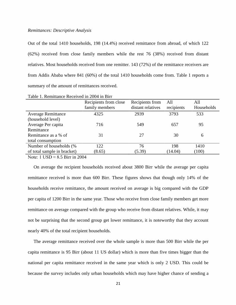
Remittances: Descriptive Analysis

Out of the total 1410 households, 198 (14.4%) received remittance from abroad, of which 122

(62%) received from close family members while the rest 76 (38%) received from distant

relatives. Most households received from one remitter. 143 (72%) of the remittance receivers are

from Addis Ababa where 841 (60%) of the total 1410 households come from. Table 1 reports a

summary of the amount of remittances received.

Table 1. Remittance Received in 2004 in Birr

Recipients from close

family members

Recipients from

distant relatives

All

recipients

All

Households

Average Remittance

(household level)

4325 2939 3793 533

Average Per capita

Remittance

716 549 657 95

Remittance as a % of

total consumption

31 27 30 6

Number of households (%

of total sample in bracket)

122

(8.65)

76

(5.39)

198

(14.04)

1410

(100)

Note: 1 USD ≈ 8.5 Birr in 2004

On average the recipient households received about 3800 Birr while the average per capita

remittance received is more than 600 Birr. These figures shows that though only 14% of the

households receive remittance, the amount received on average is big compared with the GDP

per capita of 1200 Birr in the same year. Those who receive from close family members get more

remittance on average compared with the group who receive from distant relatives. While, it may

not be surprising that the second group get lower remittance, it is noteworthy that they account

nearly 40% of the total recipient households.

The average remittance received over the whole sample is more than 500 Birr while the per

capita remittance is 95 Birr (about 11 US dollar) which is more than five times bigger than the

national per capita remittance received in the same year which is only 2 USD. This could be

because the survey includes only urban households which may have higher chance of sending a

22

migrant member abroad and hence receiving remittance compared with households in the rural

areas. But, it may also be reflecting (at least partly) the fact that official remittance figures are

underestimated as they don’t include remittance received through informal channels.

Remittances are also big when measured as a fraction of consumption expenditure. For

remittance receivers it covers nearly one third of total consumption expenditure while it covers

6% of all households’ consumption expenditure.

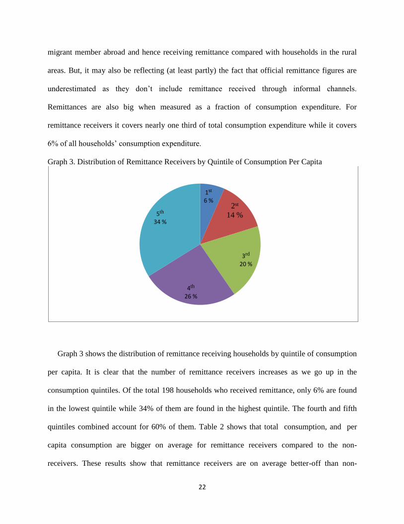
Graph 3. Distribution of Remittance Receivers by Quintile of Consumption Per Capita

Graph 3 shows the distribution of remittance receiving households by quintile of consumption

per capita. It is clear that the number of remittance receivers increases as we go up in the

consumption quintiles. Of the total 198 households who received remittance, only 6% are found

in the lowest quintile while 34% of them are found in the highest quintile. The fourth and fifth

quintiles combined account for 60% of them. Table 2 shows that total consumption, and per

capita consumption are bigger on average for remittance receivers compared to the non-

receivers. These results show that remittance receivers are on average better-off than non-

1st

6 %2st

14 %

3rd

20 %

4th

26 %

5th

34 %

23

receivers. This is not surprising considering the amount they received which is substantial as

shown in table 1. But, it is not clear if the whole effect is due to remittances or if the remittance

receiving households were better-off on average to begin with. This will be highlighted in

sections 5 and 6.

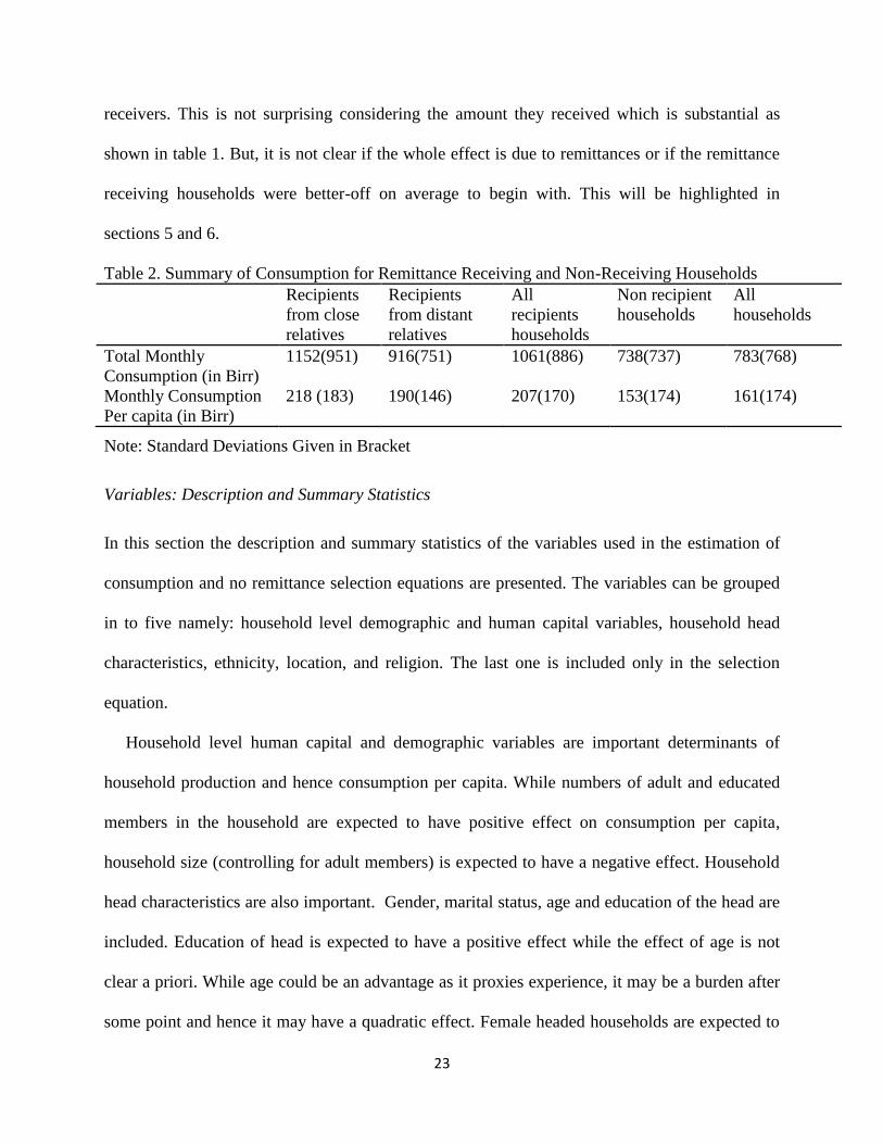
Table 2. Summary of Consumption for Remittance Receiving and Non-Receiving Households

Recipients

from close

relatives

Recipients

from distant

relatives

All

recipients

households

Non recipient

households

All

households

Total Monthly

Consumption (in Birr)

1152(951) 916(751) 1061(886) 738(737) 783(768)

Monthly Consumption

Per capita (in Birr)

218 (183) 190(146) 207(170) 153(174) 161(174)

Note: Standard Deviations Given in Bracket

Variables: Description and Summary Statistics

In this section the description and summary statistics of the variables used in the estimation of

consumption and no remittance selection equations are presented. The variables can be grouped

in to five namely: household level demographic and human capital variables, household head

characteristics, ethnicity, location, and religion. The last one is included only in the selection

equation.

Household level human capital and demographic variables are important determinants of

household production and hence consumption per capita. While numbers of adult and educated

members in the household are expected to have positive effect on consumption per capita,

household size (controlling for adult members) is expected to have a negative effect. Household

head characteristics are also important. Gender, marital status, age and education of the head are

included. Education of head is expected to have a positive effect while the effect of age is not

clear a priori. While age could be an advantage as it proxies experience, it may be a burden after

some point and hence it may have a quadratic effect. Female headed households are expected to

24

have lower consumption per capita while the effect of marital status is not clear. Location and

ethnic variables are also included. While location reflects the variation in economic activities and

cost of life across regions, the ethnicity variables will capture any difference among ethnic

groups that may affect household welfare.

The human capital and demographic variables are also important for the no remittance

selection equation. It is expected that households with more adults and educated members have

higher probability of sending a member abroad and hence lower probability of being in the no

remittance group. Not only will these household tend to have excess labor supply, they will also

have the capacity to raise fund to cover migration cost. It could also be argued that such

households will be better-off and hence have lower propensity to send a member abroad. But, as

the country is very poor the first effect is likely to dominate. Household size will have the

opposite effect. Household head characteristics could also be important. Location which is

associated with economic opportunities and cost of migration is very important. For example,

households from Addis Ababa are expected to have lower chance of being in the no remittance

group compared to households from other cities because migration cost is lower for households

living in Addis Ababa.

As the social-capital theory of migration posits, social networks are also important

determinants of migration. More specifically, households who are members of a bigger

community that has long tradition of migration will be more likely to migrate. Migration

networks could be formed along different lines and a case in point is ethnicity. Households from

ethnic groups with long migration tradition will find it easier to send a member abroad and hence

have lower probability of not receiving remittance. Religion can also serve as a basis to form

social networks and hence a dummy variable for Muslim households is included. It is

25

hypothesized that Muslim households have better network with the Middle East which is a

predominantly Muslim region and is an important destination for Ethiopian emigrants. The

psychological cost of migrating to the Middle East is also lower for Muslim individuals than for

others. Hence, Muslim households are expected to have lower probability of not receiving

remittance. Religion is believed to have no direct effect on consumption and is not included in

the consumption equation. Hence, it will identify the selection equation. The list of variables and

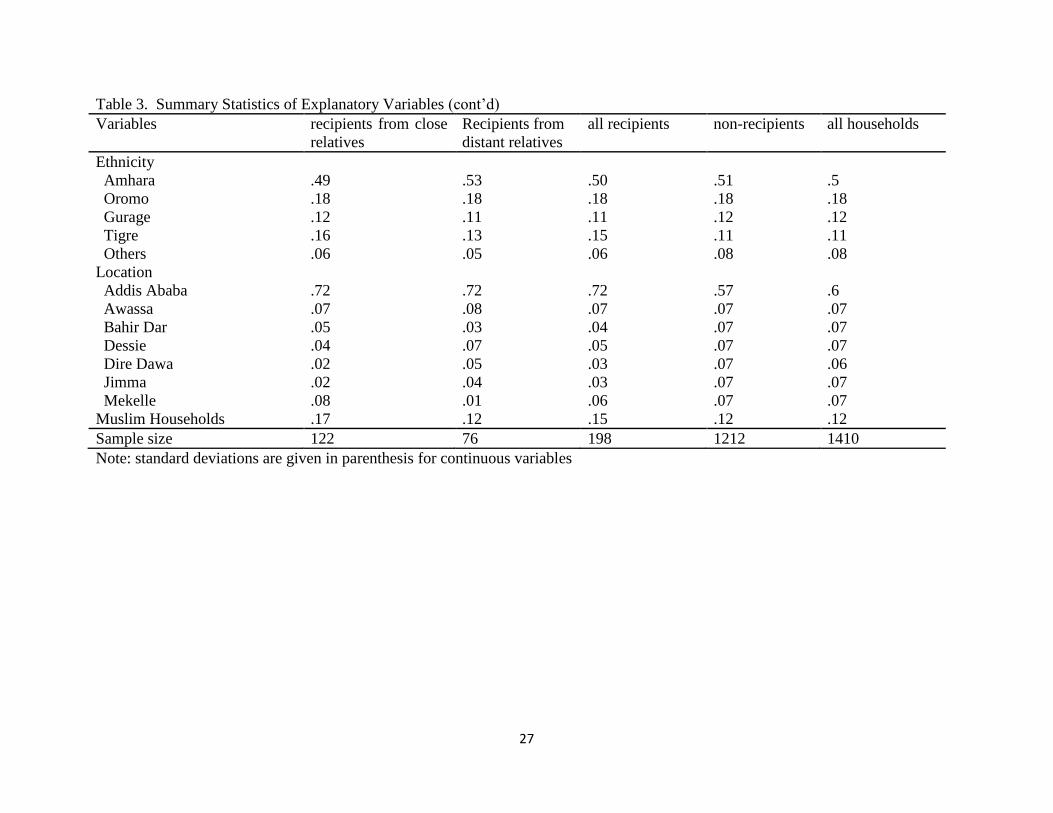
summary statistics is provided in table 3. The definitions of the variables are given in appendix.

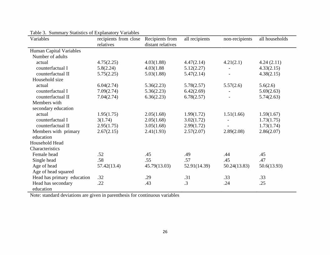
26

Table 3. Summary Statistics of Explanatory Variables

Variables recipients from close

relatives

Recipients from

distant relatives

all recipients non-recipients all households

Human Capital Variables

Number of adults

actual 4.75(2.25) 4.03(1.88) 4.47(2.14) 4.21(2.1) 4.24 (2.11)

counterfactual I 5.8(2.24) 4.03(1.88 5.12(2.27) - 4.33(2.15)

counterfactual II 5.75(2.25) 5.03(1.88) 5.47(2.14) - 4.38(2.15)

Household size

actual 6.04(2.74) 5.36(2.23) 5.78(2.57) 5.57(2.6) 5.6(2.6)

counterfactual I 7.09(2.74) 5.36(2.23) 6.42(2.69) - 5.69(2.63)

counterfactual II 7.04(2.74) 6.36(2.23) 6.78(2.57) - 5.74(2.63)

Members with

secondary education

actual 1.95(1.75) 2.05(1.68) 1.99(1.72) 1.51(1.66) 1.59(1.67)

counterfactual I 3(1.74) 2.05(1.68) 3.02(1.72) - 1.73(1.75)

counterfactual II 2.95(1.75) 3.05(1.68) 2.99(1.72) - 1.73(1.74)

Members with primary

education

2.67(2.15) 2.41(1.93) 2.57(2.07) 2.89(2.08) 2.86(2.07)

Household Head

Characteristics

Female head .52 .45 .49 .44 .45

Single head .58 .55 .57 .45 .47

Age of head 57.42(13.4) 45.79(13.03) 52.91(14.39) 50.24(13.83) 50.6(13.93)

Age of head squared

Head has primary education .32 .29 .31 .33 .33

Head has secondary

education

.22 .43 .3 .24 .25

Note: standard deviations are given in parenthesis for continuous variables

27

Table 3. Summary Statistics of Explanatory Variables (cont’d)

Variables recipients from close

relatives

Recipients from

distant relatives

all recipients non-recipients all households

Ethnicity

Amhara .49 .53 .50 .51 .5

Oromo .18 .18 .18 .18 .18

Gurage .12 .11 .11 .12 .12

Tigre .16 .13 .15 .11 .11

Others .06 .05 .06 .08 .08

Location

Addis Ababa .72 .72 .72 .57 .6

Awassa .07 .08 .07 .07 .07

Bahir Dar .05 .03 .04 .07 .07

Dessie .04 .07 .05 .07 .07

Dire Dawa .02 .05 .03 .07 .06

Jimma .02 .04 .03 .07 .07

Mekelle .08 .01 .06 .07 .07

Muslim Households .17 .12 .15 .12 .12

Sample size 122 76 198 1212 1410

Note: standard deviations are given in parenthesis for continuous variables

28

For the first three variables in the human capital and demographic category, two

counterfactuals are provided for remittance receiving households along with the actual values.

The first counterfactual (counterfactual I) includes remitters who are close family members while

the second counterfactual (counterfactual II) assumes that every remittance receiving household

has one migrant member. In both cases a migrant is assumed to be an adult (older than 14 years

old) and with high school education. The counterfactuals are used in the first stage selection

regression and in calculating the counterfactual consumptions.

Big differences are observed for some of the variables between remittance receiving and non-

receiving households. The recipient group are on average larger, have more adults and high

school graduates. This is true even for the actual values which do not take in to account migrant

members though the difference becomes smaller. The proportion of households with female,

single and high school graduate heads is also larger for remittance receiving group who also have

older heads on average. When it comes to ethnic groups, the proportion of Amharas, Oromos,

and Gurages is similar in the receiving and non-receiving groups. Tigres are overrepresented

while other ethnic groups are underrepresented in the recipient group.

Proportionally higher number of households from Addis Ababa receives remittance. While

Addis Ababa’s share in the whole sample is 60% it accounts for 72% of the remittance receiving

households. The other cities have lower shares in the remittance receiving group than their shares

in the whole sample with the exception of Awassa which has the same share of remittance

receivers as its share of the total sample. The fact that Addis Ababa has higher proportion of

remittance receiving households than the other cities is to be expected as it is easier for

households living in Addis Ababa to send members abroad and hence receive remittance

compared to households in regional cities. The fraction of Muslim households is bigger for the

29

recipient group. Differences are also observed in some of the variables between the two

remittance receiving groups. For example, those who receive remittance from close family

members have on average larger adult members and household size than the group that receives

remittance from distance relatives.

IV. Regression Results

In this section the regression results which will be used to construct counterfactual consumption

for remittance receiving households are presented. As discussed in section three, the two step

Heckman selection method is used. While only information from non-remittance receiving

households is used for the consumption estimation, in the first stage selection equation (in to no

remittance) all households are included. In the selection equation, the household human capital

and demographic variables for the remittance receiving households are adjusted so that they will

include the migrant members. Two alternative assumptions are made. In the first assumption

(Assumption I), only remitters who are close family members are included while in the second

assumption (Assumption II) one member is added for all households who received remittance.

Hence, two regression equations are estimated (one for each assumption) and the results of both

regressions are reported in table 4. All remittance receiving households are included in the

selection group in both regressions. Though the results of the two regressions are similar in

general some differences are observed. The result based on Assumption I is discussed first and

the differences with the second regression are mentioned later.

30

Table 4. Estimates of Selection Controlled Counterfactual Consumption Regression

Explanatory Variables

Assumption I Assumption II

Log Consumption

per capita

P(No Remittance) Log Consumption

per capita

P(No Remittance)

Number of adults .031(.023) .077(.05) .015(.022) -.039(.05)

Household size -.151(.021)*** .021(.052) -.17(.024)*** -.102(.05)***

Members with primary educ .022(.022) -.1(.051)** .051(.023)** .103(.05)***

Members with secondary educ .047(.041) -.375(.052) *** .067(.029)** -.154(.051)**

Female head -.141(.06)** .025(.132) -.15(.061)** -.041(.133)

Single head .069(.066) -.327(.129)** .044(.07) -.397(.13)***

Age of head .018(.01)* .035(.019)* .019(.01)* .035(.019)*

Age squared of head -.000(.000) -.000(.000)** -.000(.000) -.000(.000)**

Head has primary education .288(.039)*** .092(.134) .253(.001)*** -.145(.134)

Head has secondary education .569(.077)*** .266(.156) * .533(.073)*** -.029(.155)

Awassa .201(.086)** -.198(.19) .204(.087)** -.141(.19)

Bahir Dar .317(.086)*** .265(.214) .333(.089)*** .329(.22)

Dessie -.181(.083)** .219(.208) -.181(.086)** .193(.208)

Dire Dawa -.128(.087) .427(.231)* -.127(.088) .401(.232)*

Jimma .015(.086) .451(.232)* .022(.087) .449(.233)*

Mekelle .207(.129) .234(.258) .207(.13) .196(.257)

Amhara .009(.084) -.371(.217)* -.000(.086) -.375(.217)*

Oromo -.091(.095) -.047(.239) -.093(.097) -.056(.238)

Gurage -.000(.09) -.339(.227) -.004(.092) -.324(.226)

Tigre -.117(.133) -.69(.266)*** -.13(.134) -.662(.266)**

Muslim -.54(.15)*** -.512(.149)***

Constant 4.43(.256)*** 1.32(.54)** 4.476(.252)*** 1.753(.547)***

Lambda .453(.276)* .567(.274)**

Note: Standard errors are given in parenthesis. *, **, and *** represent significance level at 10%, 5% and 1% respectively

31

In the first stage selection equation, two of the household human capital variables namely

number of household members with primary and high school education are significant. Both

affect the probability of not receiving remittance negatively. In other words, they positively

affect the probability of having a migrant relative abroad and hence receiving remittance as

expected. It is also worth noting that the coefficient for members with high school education is

bigger than the coefficient for members with primary education.5

Coming to the household head characteristics, having a single head is associated with lower

probability of not receiving remittance while age of head has an opposite effect (though

significant only at ten percent level). The squared age of the head has a significant negative

effect but its coefficient is approximately zero. Households with heads who are high school

graduates have higher chance of not receiving remittance. This is in contrast with the effect of

members with high school education. The fact that the head has a high school education may

show that s/he has a good and stable income and hence the need to send a member abroad and

receive remittance will be lower while having more educated household members means more

labor is available in the households and part of it can be allocated abroad.

From the city dummies only Dire Dawa and Jimma have significant effects. Both have

positive coefficients implying that households from these places are more likely to be non-

remittance recipients compared to households from Addis Ababa. Two of the ethnic dummies

namely Amharas and Tigres also have negative and significant coefficients. This shows that the

two ethnic groups are less likely to be in the selection group of no remittance compared with the

reference group which includes ethnicities other than the four major ethnic groups. Amharas and

Tigres are mainly found in the northern part of Ethiopia which is close to the Middle East (and

5 It could be argued that remittance might affect some of the household level demographic and human capital

variables. But, given that most of the remitters stayed abroad only for few years, the average being 7 years, it is believed that there will not be big endogeneity bias.

32

Europe) and they might have longer migration history than the other ethnic groups. War, draught

and famine have also been more common in the north which might have led to more migration in

the past. Finally, Muslim households have lower probability of not receiving remittances as

expected. The fact that the coefficient is highly significant and big in absolute terms compared to

the other coefficients shows that religion is important in determining households’ selection in to

the non-remittance receiving group. Religion is not included in the second stage consumption

equation and hence identifies the selection equation.

Turning in to the consumption equation, the first thing to observe is that the Lambda has a

significant (at 10% level) and positive coefficient showing that errors of the two equations (no

remittance and consumption) are positively correlated or non-remittance receiving households

are positively selected in their unobservable characteristics. To put it differently, there is

negative selection in to migration and remittance. Though this is against the usual belief that

migrant households are positively selected, it is consistent with the finding by Acosta et al (2008)

in Latin America and Gubert et al (2010) in Mali. Thus, counterfactual estimation which does

not take selection in to account will underestimate the effect of remittance on consumption.

From the human capital variables, only household size has significant effect on consumption

per capita. The coefficient is negative implying that per capita consumption decreases with

household size. This is not surprising as household size includes children who normally do not

contribute much to the household income. But, it is worth mentioning that number of adults and

educated members do not have significant effects (controlling for household size) which reflects

the limited employment opportunity in the country. From the household head characteristics;

gender, age and education of head are important. Female headed households have lower

consumption per capita while age and education of head increases consumption per capita. From

33

the city dummies, Awassa and Bahir Dar are associated with higher consumption per capita

relative to Addis Ababa. The two cities, though found on different sides of Addis Ababa are

similar in that both are found in regions with rich agricultural potential. None of the ethnic

dummies are significant.

Though the results based on Assumption II are basically similar some differences are

observed both in the selection and consumption equations. In the selection equation, household

size becomes significant with a negative effect on the likelihood of being in the non-remittance

receiving group. Number of household members with primary education has now a positive

effect on the probability of being in the non-remittance group. On the other hand, whether the

household head has a high school education or not does not matter. In the consumption equation,

numbers of household members with primary and high school education become significant with

positive effects. In Assumption I, they were not significant though they had similar sign. The

presence of selection is stronger in assumption II where the hypothesis that there is no selection

is rejected at 5% level.

The consumption estimates presented in table 4 will be used to construct counterfactual

consumption values for remittance receiving households in the hypothetical case of no migration

and no remittance. Like in the estimation of the selection equation, the household human capital

variables will be updated to include the migrants. Counterfactual consumption estimates for the

remittance receiving households combined with the actual consumption values for non-receivers

will constitute the consumption distribution in case of no migration and no remittance. But, a

problem arises namely that the counterfactual values for the remittance receiving households are

based on observable characteristics and hence have an artificially reduced variance. As a result,

the counterfactual and actual consumption distributions are not comparable. To fix this problem

34

an OLS regression is run on the whole sample and the result is used to predict consumption in

the actual case as is discussed in section three. This way, the two distributions will be

comparable. The result is reported in table 5.

Table 5. OLS estimates of actual consumption regression (log consumption per capita)

Explanatory variables Slope coefficients

(standard errors in bracket)

Number of adults .031(.019)

Household size -.158(.019)***

Members with primary education .032(.019)*

Members with secondary education .091(.021) ***

Female head -.139(.052)***

Single head .093(.052)*

Age of head .006(.008)

Age squared of head -.000(.000)

Head has primary education .226(.052)***

Head has secondary education .494(.063)***

Awassa .259(.075)***

Bahir Dar .259(.076)***

Dessie -.192(.075)***

Dire Dawa -.157(.077)**

Jimma -.017(.075)

Mekelle .134(.108)

Amhara .029(.074)

Oromo -.094(.085)

Gurage .027(.079)

Tigre -.016(.105)

Remittance .441(.065)***

Remittance from distance relatives -.242(.098)**

Constant 4.77(.212)***

Adjusted R-squared .28

Note: *, **, and *** represent significance level at 10%, 5% and 1% respectively

Most of the variables that were significant in the selection controlled consumption regression

are significant also now with similar sign. The two remittance variables are highly significant.

The coefficient for the first remittance variable shows that households who receive remittance

from close relatives have on average 44% higher per capita consumption than those who don’t

35

receive remittance. The second remittance variable has a negative coefficient and shows that

households who receive remittance from distance relatives have 24% less consumption per capita

compared to those who receive from close relatives, i.e., remittance from distance relatives leads

to a 20% rise in consumption per capita compared to those who do not receive any remittance.

The effects of both types of remittances on consumption per capita are big and are consistent

with the result from the descriptive statistics given in the last section, i.e.; average consumption

per capita is 41% and 24% higher for households who receive remittance from close relatives

and distance relatives respectively compared to those who don’t receive remittance. Remittances

from close relatives have higher effect than remittances received from distance relatives as

expected and consistent with the fact that remittances are on average higher for the first group.

VI. Effect on Poverty and Inequality

In this section the effects of remittances on poverty and inequality are presented. The three

variants of the FGT index (Foster et al, 1984), i.e, the head count, the poverty gap and the

squared poverty gap ratios are reported. The poverty line set by Gebremedhin and Whelan

(2007) from a similar survey in 2000 is used in this paper. Following the cost of basic needs

approach they first constructed the food poverty line by estimating the value of a basket of food

items that meet the stipulated minimum calorie requirement for a healthy life which is 2200 Kcal

per adult per day. Then, the food poverty line was scaled up to include the non-food component

taking in to account the share of food consumption expenditure. Accordingly, the total poverty

line per adult per month was 91 Birr in 2000 which becomes 100.24 Birr after adjusting for

inflation between 2000 and 2004. For the inequality analysis the Gini index is used. The

consumption shares of the top 20% and bottom 20% of the households ranked by consumption

per capita (and their ratio) are also used as complementary measures of inequality. The Gini and

36

the three poverty indices are calculated using household consumption per capita adjusted by

equivalence scale.6 Household sizes are used as weights. The equivalence scale used takes in to

account the fact that children cost less than adults and there is economies of scale in

consumption. It is given as follows:

,0 1,0 1 (6)ES A K

Where ES is equivalence scale, A is number of adults, K is number of children, α is cost of

children relative to adults and θ is a measure of economies of scale. It is believed that α is low

and θ high in poor countries, i.e., while children cost low relative to adults there is no much

economies of scale in poor countries (Deaton and Zaidi, 1998). Following Kedir and Disney

(2004) α and θ are respectively set to be 0.5 and 0.95.

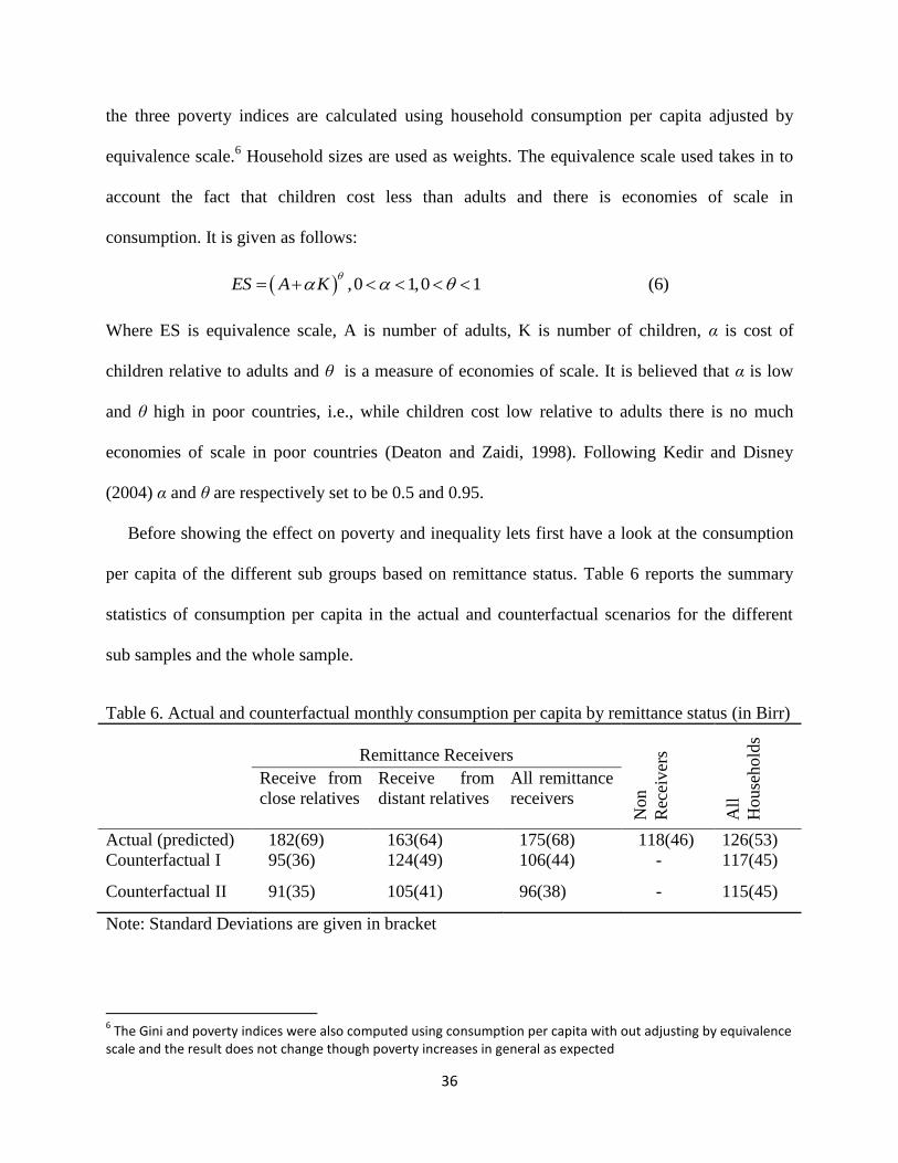
Before showing the effect on poverty and inequality lets first have a look at the consumption

per capita of the different sub groups based on remittance status. Table 6 reports the summary

statistics of consumption per capita in the actual and counterfactual scenarios for the different

sub samples and the whole sample.

Table 6. Actual and counterfactual monthly consumption per capita by remittance status (in Birr)

Remittance Receivers

Non

Rec

eiver

s

All

House

hold

s

Receive from

close relatives

Receive from

distant relatives

All remittance

receivers

Actual (predicted) 182(69) 163(64) 175(68) 118(46) 126(53)

Counterfactual I 95(36) 124(49) 106(44) - 117(45)

Counterfactual II 91(35) 105(41) 96(38) - 115(45)

Note: Standard Deviations are given in bracket

6 The Gini and poverty indices were also computed using consumption per capita with out adjusting by equivalence

scale and the result does not change though poverty increases in general as expected

37

As can be seen from table 6 consumption per capita is higher for remittance receivers than for

the non-receivers in the actual case while it is lower in the two counterfactuals. This implies that

the non-recipients are on average better off than the receivers in the absence of remittance which

is consistent with the negative selection in to migration and remittance found in the last section.

From the two remittances receiving groups, the average actual consumption per capita is larger

for the group that receives from close relatives. The opposite is true in the two counterfactuals.

Average consumption per capita is higher under counterfactual I than under counterfactual II for

both groups of remittance recipients though the difference is small for those who receive from

close relatives. For the group that receives remittance from distant relatives average consumption

per capita is substantially bigger in counterfactual I which is based on the assumption that these

households do not have migrant members and they just receive remittance from individuals who

were not part of the household before they migrate. This may sound counterintuitive but it is

consistent with the selection controlled consumption estimates presented in the last section. Even

if having an additional adult member with a high school education has a positive effect on

consumption per capita, the effect of an additional household size is negative and stronger. This

implies that having an additional household member does not increase household welfare. This

reflects the low employment opportunity available at home even for those with high school

education.

38

Graph 4. Distribution of Remittance Receivers by Quintile of Actual and Counterfactual

Consumption per capita

Graph 4 shows the distribution of remittance receivers by quintile of actual and counterfactual

consumption per capita. It is clearly seen that remittance receivers are concentrated in the higher

quintiles in the actual case while the opposite is true under the two counterfactuals. In the actual

case about 5% of the remittance receivers come from the lowest quintile while more than 50%

come from the highest quintile. Based on counterfactual I, 30% of them come from the first

quintile and only 13% come from the highest quintile. The result for counterfactual II is similar.

Next let’s see the effect on poverty and inequality.7 Table 7 reports the effect on the remittance

receiving group.

7 The poverty and inequality values are calculated using bootstrap method

0,00

10,00

20,00

30,00

40,00

50,00

60,00

1 2 3 4 5

% of

Rem

itta

nce

Rec

eiver

s

Quintile

Actual Counterfactual1 Counterfactual2

39

Table 7. Effect on Poverty and Inequality on Remittance Receivers

Head Count

Ratio

Poverty Gap

Ratio

Squared Poverty

Gap Ratio

Gini

Coefficient

Receive

from

close

relatives

Actual .042 .005 .001 .206

Counterfactual I .527 .128 .043 .206

Difference ↓.485(92%) ↓.123(96%) ↓.042 (98%) .000(0%)

Counterfactual II .562 .153 .057 .210

Difference ↓.520(93%) ↓.148(97%) ↓.056(98%) ↓.004(19%)

Receive

from

distant

relatives

Actual .086 .010 .001 .201

Counterfactual I .238 .039 .010 .203

Difference ↓.152(64%) ↓.029(74%) ↓.009(90%) ↓.002(1%)

Counterfactual II .462 .094 .027 .207

Difference ↓.376(81%) ↓.084(89%) ↓.026(99.6%) ↓.006(3%)

All

remittance

receivers

Actual .058 .007 .001 .206

Counterfactual I .433 .099 .033 .218

Difference ↓.375(87%) ↓.092(93%) ↓.032(97%) ↓.012(5.5%)

Counterfactual II .525 .131 .046 .213

Difference ↓.467(89%) ↓.124(95%) ↓.045(98%) ↓.005(2.3%)

Non

Receivers

Actual .286 .062 .021 .210

As can be seen from table 7, remittances have substantially reduced poverty among the

recipient group. The head count, the poverty gap and the squared poverty gap ratios are

respectively 52.5%, 13.1% and 4.6% in counterfactual II, 43.3%, 9.9% and 3.3% in

counterfactual I and 5.8%, 0.7% and 0.1% in the actual case. The poverty levels in the two

counterfactuals are considerably higher than the poverty levels for the non-recipient group

implying that poverty was higher among the receivers before migration. But, in the actual case

which includes the effect of remittance, poverty is very low for the remittance receivers. This

shows how important remittances are in lifting households out of poverty in Ethiopia. Poverty is

40

larger in counterfactual II which also means the poverty reduction rate is higher. This holds for

the two groups though the effect as was found in the summary of consumption per capita is more

pronounced for the group of households who receive remittance from distant relatives. It is also

noteworthy that the rate of poverty reduction is higher for the poverty gap and squared poverty

gap ratios than for the head count ratio. The effect on inequality is negligible though remittance

is associated with a slight fall in inequality. The inequality levels for remittance receivers and

non-receivers are also comparable. The effect on the whole sample is reported in table 8.

41

Table 8. Effect on Poverty and Inequality on the whole sample

Actual Counterfactual I Difference Counterfactual II Difference

Poverty head count ratio .253 .309 ↓.053(17%) .326 ↓.070(21%)

Poverty Gap .054 .068 ↓.014(21%) .074 ↓.020(27%)

Squared Poverty Gap .018 .023 ↓.005(23%) .025 ↓.007(28%)

Gini Index .225 .212 ↑.013(6%) .214 ↑.011(5%)

Share of top 20% .331 .322 ↑.009(3%) .323 ↑.008(2%)

Share of bottom 20% .105 .108 ↓.003(3%) .107 ↓.002(2%)

Ratio of share of top 20% to

share of bottom 20%

3.15 2.98 ↑.17(6%) 3.02 ↑.13(4%)

Note: The top 20% and the bottom 20% consumption shares are calculated after households are ranked by consumption per capita

42

Comparing the poverty measures in the two counterfactual cases with the actual one shows

that poverty has decreased considerably. The head count ratio in counterfactual I is 30.9% and

decreased to 25.3% in the actual case representing a substantial 17% fall in poverty. Similarly

the poverty gap ratio decreased by 21% from 6.8% to 5.4% while the squared poverty gap ratio

droped by 23% from 2.3% to 1.8%. The fall in poverty is even bigger if counterfactual II is

considered. The reduction in poverty is remarkable taking in to account only 14% of households

get remittance. Poverty decreased significantly because remittance receivers mainly come from

the bottom income distribution as reflected by their low average consumption in the

counterfactual cases. Besides, the remittance they received is big enough to lift many of them out

of poverty.

Though remittance seems to have worsened inequality the magnitude is negligible. If

counterfactual I is considered the Gini coefficient increased from 21.2% to 22.5%. The

consumption share of the top 20% increases from 32.2% to 33.1% while the share of the bottom

20% slightly fall from 10.8% to 10.5%. The result for counterfactual II is similar. Given that

remittance receivers were on average poorer than the non-receivers in the absence of remittance

and inequality with in the recipient group is reduced slightly, one would expect a reduction in

inequality as well. But, the fact that the amount received is big (relative to the average

consumption) means remittances also have unequalizing effect. This is reflected in the actual

average consumption of remittance receivers which is bigger than the average consumption for

non-receivers. The result suggests that the two opposing effects nearly cancel out.

V. Conclusion

The paper studies the impact of remittances on poverty and inequality in Ethiopia using urban

household survey. Counterfactual consumption is estimated in the hypothetical case of no

43

migration and no remittance using information on the non-remittance receivers in a selection

corrected estimation framework which incorporates migration decision by households. In the

absence of detailed information about the remitters two assumptions were made while

constructing the hypothetical consumption distributions. In the first counterfactual only remitters

who are close family members were included in the households while in the second

counterfactual all remittance receiving households were assumed to have one migrant member

abroad. The result shows that remittance receivers have lower consumption per capita than the

non receivers in the counterfactual scenarios while they have higher consumption per capita in

the actual case. The selection result also shows that remittance receiving households are

negatively selected in their unobservable characteristics.

Poverty substantially decreased for the group of remittance receiving households which also

led to a big fall in overall poverty. Based on the first assumption, the head count ratio for the

whole sample fell from 30% to 25% representing 17% reduction in poverty. The poverty gap

ratio decreased from 6.8% to 5.4% showing a 21% decrease. The squared poverty gap ratio

dropped by 23%. Poverty even decreased more when the second assumption is used. The fall in

poverty is high given that only 14% of the households receive remittance and two explanations

could be given for this. First, remittance receiving households on average come from the lower

consumption distribution. Second, the remittance they receive on average is substantially big

relative to the average consumption in the sample.

The effect on inequality is negligible though a slight rise is observed. Given that remittance

receivers come from the lower consumption distribution inequality would be expected to fall.

But since remittances are big compared to the average consumption in the sample they might

44

also have unequalizing effect. The result suggests that the two effects nearly cancel out and

hence no big effect on inequality.

Taking in to account that Ethiopia does not have long migration history, the result on poverty

is remarkable and contradicts the hypothesis that remittances do not have significant poverty

reducing effect in a country with out long migration history because migration in such situation

is risky and expensive and hence only the better-off households can afford it. The lack of strong

migration networks coupled with the extremely low average income in Ethiopia also suggests

that remittances will worsen inequality significantly which was not the case. But, given the low

employment opportunity and the high poverty level in Ethiopia migration may not be considered

as a risky investment. There are anecdotal evidences that many young men and women try to go

abroad in illegal means which involves huge risk in search of better opportunities. On top of that,

once there is a prospect for a household member to go and work abroad, the household in

collaboration with other households in the extended family might have an informal mechanism

of raising fund to cover the migration cost. But, to understand the situation well a detailed study

is required including on how migration costs were financed. It is also interesting to disaggregate

the effect by major destinations of Ethiopian emigrants.

45

References

Acosta P. (2006), “Labor Supply, School Attendance, and Remittances from International

Migration: The case of El Salvador”, World Bank Policy Research Working Paper, WPS3903

Acosta P., C. Calderon, P.Fajnzylber and H. Lopez (2008), “What is the Impact of International

Remittances on Poverty and Inequality in Latin America?”, World Development, Vol. 36,

No. 1, pp. 89-114

Adams R.H.Jr (1989), “Workers Remittances and Inequality in Rural Egypt”, Economics

Development and Cultural Change, Vol. 38, No.1, pp. 45-71

Adams R.H.Jr. (2005), “Remittance, Poverty and Investment in Guatamala”, in International

Migration, Remittances and the Brain Drain, Ozden C., and M. Schiff (eds),

The World Bank Washington D.C.

Adams R.H. Jr (2006), “Remittance and Poverty in Ghana”, World Bank Policy Research

Working Paper 3838, February 2006

Adams R.H.Jr. and J. Page (2005), “Do International Migration and Remittances Reduce Poverty

in Developing Countries?”, World Development Vol.33, No.10, pp. 1645-1669

Anbesse B., C. Hanlon, A. Alem, S. Packer and R. Whitley (2009), “Migration and Mental

Health: a Study of Low-Income Ethiopian Women Working in Middle Eastern Countries”,

International Journal of Social Psychiatry, Vol. 55

Anyanwu J.C. and A.E.O.Erhijakpor (2010), “Do International Remittances Affect Poverty in

Africa?”, African Development Review, Vol. 22, No.1, pp 51-91

Bradford B.and S. Boucher (1998), “Migration, Remittances, and Inequality: Estimating the net

effect of Migration on Income Distribution”, Journal of Development Economics, Vol. 55,

No. 2, pp. 307-331

46

Cameron, A.C. and P.K. Trovedi (2005), Microeconometrics: Methods and Applications,

Cambridge University Press

Cramer C. (2003), “Does inequality cause conflict” Journal of International Development Vol.

15, pp. 397-412

Deaton A. (1997), The Analysis of Household Surveys: A Micro-economic Approach to

Development Policy, The Johns Hopkins University Press

Deaton A,. and S. Zaidi (1999), Guidelines for Constructing Consumption Aggregates For

Welfare Analysis, Washington D.C., The World Bank

Edwards A.C. and M. Ureta (2003), “International migration, remittances, and schooling:

evidence from El Salvador”, Journal of Development Economics, Vol. 72, No. 2, pp. 429-461

Easterly W. (2007), “Inequality does cause underdevelopment: Insights from a new Instrument”,

Journal of Development Economics, Vol.84, No.2, pp.755-776

Foster J, J.Greer and E.Thorbecke (1984), “A Class of Decomposable Poverty Measures”,

Econometrica, Vol. 52, No.3, pp. 761-766

Fransen S. and K. Kuschminder (2009), “Migration in Ethiopia: History, Current Trends and

Future Prospects”, Paper Series: Migration and Development Country Profile, Maastricht

Graduate School of Governance (MGSoG)

Furman J. and J.E.Stiglitz (1998), “Economic Consequences of Income Inequality” In Income

inequality: issues and policy options. Kansas City: Federal Reserve Bank of Kansas City

Gebremedhin T.A, and S. Whelan, (2007), “Prices and Poverty in Urban Ethiopia”, Journal of

African Economies, Vol. 7, No 1, pp. 1-33

Glaeser E., J.Scheinkman and A. Shleifer (2003), “The injustice of inequality”, Journal of

Monetary Economics, Vol.50, pp. 199-222

47

Gonzalez – Konig G. and Q.Wodon (2005), “Remittances and Inequality”, Department of

Economics and Finance Working Paper, EC200506, Universidad de Guanajuato

Grigorian D.A. and T.A.Melkonyan (2008), “Microeconomic Implications of Remittances in an

Overlapping Generations Model with Altruism and Self-Interest”, IMF Working Paper,

WP/08/19

Gubert F., T.Lassourd and S.Mesple-Somps (2010), “Do Remittances Affect Poverty and

Inequality? Evidence from Mali”, Document De Travel DT/2010-08, Paris-Dauphine

University

Gustafsson B. and N. Makonnen (1993), “Poverty and Remittances in Lesotho”, Journal of

African Economies, Vol.2, No.1, pp.49-73

Heckman J.J. (1979), “Sample Selection Bias as a Specification Error”, Econometrica, Vol.47,

No. 1, pp. 153-161

Kebede, Emebet (2002), “Ethiopia: An assessment of International Labor Migration Situation.

The case of Female Migrants” GENPROM Working Paper, No. 3, Geneva:

International Labour Organization

Kedir A.M, and R.Disney (2004), “Prices in the Measurement of Food Poverty in Urban

Ethiopia”, Paper presented at the First International Conference on the Ethiopian Economy

Koechlin V. And G. Leon (2007), “International Remittances and Income Inequality: An

Empirical Investigation”, Journal of Economic Policy Reform, Vol.10, No.2, pp. 123-141

Mckenzie D. and H. Rapoport (2007), “Network effects and the dynamics of migration and

inequality: Theory and evidence from Mexico”, Journal of Development Economics, Vol. 84,

Issue 1, pp. 1-24

Massey D.S. (1990), “Social Structure, Household Strategies, and the Cumulative Causation of

Migration”, Population Index, Vol.56, No.1, pp. 3-26

48

Massey D.S. and K.E. Espinosa (1997), “What’s Driving Mexico-U.S. Migration? A

Theoretical, Empirical, and Policy Analysis”, The American Journal of Sociology, Vol. 102,

No.4, pp. 939-999

Ravallion M. (2001), “Growth, inequality and poverty: Looking Beyond Averages”, World

Development, Vol.29, No.11, pp.1803-1815

Ravallion M. (2005), “Inequality is bad for the poor”, World Bank Policy Research Working

Paper 3677

Richard B.P.C. and E. Jimenez (2008), “Estimating the Net-effect of Migration and Remittances

on Poverty and Inequality: Comparison on Fiji and Tonga”, Journal of International

Development, Vol. 20, No.4, pp. 547-571

Rodriguez E.R. (1998), “International Migration and Income Distribution in the Philippines”,

Economic Development and Cultural Change, Vol.46, No.2, pp. 329-350

Shen I., F.Docquier and H.Rapoport (2010), “Remittance and Inequality: a Dynamic Migration

Model”, Journal of Economic Inequality, Vol.8, No.2, pp. 197-220

Stark O., T.E.Taylor and S.Yitzhaki (1986), “Remittances and Inequality”, The Economic

Journal, Vol. 96, No. 383, pp. 720-740

Taylor J.E., J.Mora, R. Adams, A. Lopez-Feldman (2005), “Remittances, Inequality and Poverty:

Evidence from Rural Mexico”, Working Paper No. 05-003, Giannini Foundation for

Agricultural Economics

United Nations Development Program (2009), Human Development Report. Overcoming

Barriers: Human Mobility and Development, UNDP, New York

World Bank (2011), Migration and Remittances Fact Book 2011, 2nd

ed, The World Bank,

Washington DC

49

World Bank, World Development Indicators (various years): http://data.worldbank.org/indicator

Yang D. and C.Martinez (2005), “Remittances and Poverty in Migrants’ Home Areas:

Evidence from the Philippines”, in International Migration, Remittances and the Brain Drain,

Ozden C., and M. Schiff (eds), The World Bank Washington D.C.

Yang D. and H. Choi (2007), “Are Remittances Insurance? Evidence from Rainfall Shocks in

the Philippines”, The World Bank Economic Review, Vol. 21, No.2, pp. 219-248

50

Appendix

Table 9. Definitions of Variables

Variables Definition

Human Capital Variables

Number of adults Number of adult in the households

Household size Household size

Members with

secondary education

Number of household members who have

completed high school

Members with primary education Number of household members who have

completed primary education

Household Head

Characteristics

Female head Dummy for female household heads

Single head Dummy for single household heads

Age of head Age of household head in years

Age of head squared Age of household head squared

Head has primary education Dummy for household heads who have

completed primary education

Head has secondary education Dummy for household heads who have

completed high school education

Ethnicity (control group: other ethnic groups)

Amhara Dummy for Amhara households

Oromo Dummy for Oromo households

Gurage Dummy for Gurage houseolds

Tigre Dummy for Tigre households

Location (control group: Addis Ababa)

Awassa Dummy for households from Awassa

Bahir Dar Dummy for households from Bahir Dar

Dessie Dummy for households from Dessie

Dire Dawa Dummy for households from Dire Dawa

Jimma Dummy for households from Jimma

Mekelle Dummy for households from Mekelle

Muslim Households Dummy for Muslim households