the effect of investment constraints on hedge fund ... annual meetings/2014-… · hedge fund...
TRANSCRIPT

The Effect of Investment Constraints on
Hedge Fund Investor Returns
JUHA JOENVÄÄRÄ, ROBERT KOSOWSKI, and PEKKA TOLONEN*
This Version: 8 January 2014
ABSTRACT
The aim of this paper is to examine the effect of frictions and real-world investment constraints
on the returns that investors can earn from investing in hedge funds. We contribute to the
existing literature by accounting for share restrictions, minimum diversification requirements and
fund size restrictions that are commonly used by institutional investors. We show that the size-
performance relationship is positive (negative) when past (future) performance is used. Evidence
of performance persistence is reduced significantly when fund size and share restrictions such as
notice, redemption and lockup period are incorporated into rebalancing rules. We test several
hypotheses regarding the economic mechanism that underlies the size-performance relationship.
We find empirical support for theoretical models based on decreasing returns to scale as well as
managers responding optimally to fee incentives. The findings have significant implications for
hedge fund investors since they caution against chasing performance in hedge funds and within
the billion dollar club of hedge funds, in particular.
* We would like to thank Magnus Dahlqvist, Petri Jylhä, Niklas Kohl, Tarun Ramodorai and seminar participants at
the 8th Annual Conference on Advances in the Analysis of Hedge Fund Strategies 2013, the 2013 NBIM Financial
Research Conference in Oslo, Stockholm School of Economics, the 2013 Young Scholars Nordic Finance
Workshop inCopenhagen for helpful comments. The usual disclaimer applies. Contact addresses: Juha Joenväärä,
University of Oulu and Imperial College Business School, [email protected]. Robert Kosowski, Imperial
College Business School and Oxford-Man Institute of Quantitative Finance, [email protected]. Pekka
Tolonen, University of Oulu, [email protected].

1
I. Introduction
THE HEDGE FUND INDUSTRY has experienced a transformation and significant growth since the
financial crisis. Hedge funds‘ assets under management (AuM)1 have recovered from the lows in
2008 to reach $2.3 trillion in 2013. However, as reported in a recent Financial Times article:
There are far fewer marginal hedge funds out there because we have gone through a
period of really culling the herd. . . . The result is a calmer, if less lucrative life, both for
hedge fund managers and their investors.2
The main beneficiaries of recent investor flows have been the largest hedge fund
management companies and funds. In practice, institutional hedge fund investors face constraints
that are not just related to fund size, such as minimum fund size requirements, but also include
share restrictions (regarding notice, redemption, and lockup periods), and minimum
diversification requirements. Although the effect of investment constraints on portfolio
performance has been studied in the empirical and theoretical asset pricing literature (Figlewski
(1981), Diamond and Verrecchia (1987), Luttmer (1996)), research on hedge funds seldom
accounts for such restrictions or examines their effect on the performance of hedge fund
portfolios and the persistence of that performance.3
Our aim is to fill this research gap by documenting the effects of a combined set of
investment constraints faced by real-world hedge fund investors on their opportunity set as
indicated by historical hedge fund data over the period 1994–2012. We find that incorporating
these restrictions reduces average performance dramatically, and reduces, but does not eliminate,
performance persistence. Hence our findings support the view that return expectations of the
predominant investor type (i.e., the institutional investor) should be significantly lower than
expectations that are based on unrestricted portfolio allocations across the broader hedge fund
universe. These results call into question the practicality and implementability—from the
1 See Preqin (2013). According to our aggregate database, hedge fund AuM were $2.2 trillion in February 2013.
2 James Mackintosh, ―Transformed hedge funds in calmer waters,‖ Financial Times, 7 June 2013.
3 The paper by Edelman, Fung, and Hsieh (2012) is one of the few recent studies examining large hedge fund firms;
however, that paper does not address the effect of investment constraints on hedge fund performance and its
persistence.

2
perspective of real-world hedge fund investors—of the findings reported in previous hedge fund
studies.
Given the crucial role that fund size plays, we explore the economic mechanism
underlying the size-performance relationship. We test hypotheses about why the largest funds
attract the majority of assets, and why size is an important determinant of performance.
Investors may attempt to avoid ‗headline‘ risk associated with fund blowups and we, therefore,
test the hypothesis that larger funds have lower volatility and failure rates. It is also plausible that
larger funds optimally choose leverage to reduce the risk of drawdowns and to avoid putting
management fees at risk. Hence, we test the hypothesis that management fees as a percentage of
total fees are increasing with fund size and funds exhibit diminishing returns to scale.
Our analysis provides five key insights for investors and researchers. First, we show that
it is crucial to distinguish between the forward-looking and the backward-looking size–
performance relationship: it is the former that matters to hedge fund investors. We find that
larger funds tend to have generated higher returns than smaller funds in the past but that larger
funds tend to perform worse than smaller funds in the future. Second, we show that the higher
capital allocation to larger funds could be the result of an equilibrium in which investors avoid
the ‗headline‘ risk of smaller funds, since we find that larger funds have lower volatility and
attrition rates. Third, we find that management fees as a percentage of AuM are an increasing
function of AuM whereas performance fees are a decreasing function of AuM. This is consistent
with theories of optimal hedge fund leverage that predict that larger funds reduce leverage and
volatility in order not to put management fees at risk. Fourth, we demonstrate that fund size is
the key for the persistence of hedge fund performance. The investor‘s choice of the fund size
limit is crucial, and results for funds in the ―billion-dollar club‖ are very different from those for
smaller funds. We shed light on the economic mechanism behind differences in performance
persistence and control for the crowded trades effect using the Strategy Distinctiveness Index
(SDI) of Sun, Wang, and Zheng (2012). Our results show that strategy distinctiveness is an
important determinant of the sensitivity of future performance to past performance. Fifth,
incorporating realistic investment restrictions actually reverses widely accepted conclusions

3
about performance persistence among large hedge funds, which are the focus of institutional
investors.
The first main insight from our paper follows from examining the forward-looking size–
performance relationship for the period 1994–2012. We find that a portfolio of the largest funds
(corresponding to AuM of at least $1 billion in 2012) generates a Sharpe ratio of 0.71, which is
about half the size of the Sharpe ratio (1.34) generated by a portfolio of the smallest funds
(corresponding to AuM of less than $10 million in 2012). The Financial Times article just quoted
refers to a ―calmer life‖ for managers, and it implies that larger funds exhibit less volatility and
lower returns. This motivates us to test whether the alpha or risk-adjusted performance of larger
funds is better than that of smaller funds. We find no support for that claim, in line with several
theoretical models arguing that fund size and performance should be negatively related. The
negative forward-looking size-performance relationship is monotonic, and it holds when we take
into account various data biases such as backfill, self-selection or delisting bias.4
These findings do not bode well for the largest hedge funds and management companies,
since the reported values suggest that larger funds will be unable to continue generating superior
risk-adjusted returns. This empirical evidence is consistent with the theoretical work of
Goetzmann, Ingersoll and Ross (2003) who interpret the unwillingness of successful funds to
accept new money as indicative of diminishing returns in the hedge fund industry as a whole.
Our results are supported by the remarks of experienced hedge fund investors. A recent
Financial Times article quotes Rick Sopher (chairman of LCH Investments, the fund of hedge
funds run by the Edmond de Rothschild group), who observes that a critical component of
longer-term success for the top-20 hedge funds is to avoid becoming too big:
4 For example, out-of-sample tests using returns adjusted for backfill bias show that the largest group of funds
generates a statistically insignificant alpha of 1.4% annually. This is in sharp contrast to the corresponding returns
exhibited by our portfolio of the smallest funds, which generates an alpha of 3.9% annually (with a t-statistic of
3.36).

4
When you look at the one thing that virtually all the managers on this list have in
common, it‘s that they have all either at some point or all the way through restricted
capacity [how much money they will accept].5
Mega hedge fund management firms may point to evidence that past performance is
positively related to current fund size; however, that claim is not relevant to investors, who are
concerned with a fund‘s future performance. Our data does confirm the positive relationship
between past performance and fund size. A portfolio consisting of the (671) largest funds with
December 2012 AuM of at least $1 billion generates a Sharpe ratio of 1.56 when calculations are
based on their historical track record, whereas a portfolio of the (10,783) smallest funds
generates a Sharpe ratio of 0.66 when calculated in the same way. When we plot the forward-
looking and the backward-looking size–performance relationship in the same graph, the result is
an X-shape formed by the two lines‘ intersection.
Our second main finding is related to the economic mechanism that may underlie the
size-performance relationship. The fact that larger funds have higher AuM than smaller funds
may represent an equilibrium, because investors may wish to avoid the possibility of ―headline‖
risk, the downside of which is realized when a fund fails because of excessive risk taking or poor
operational control. Our results are consistent with this hypothesis since larger funds exhibit
lower volatility and lower attrition rates than smaller funds.
Our third main insight is related to the hypothesis that larger funds optimally choose
leverage to reduce the risk of drawdowns and to avoid putting management fees at risk. While
the models in Berk and Green (2004) and Goetzmann, Ingersoll and Ross (2003) attribute it to
diminishing returns, the optimal leverage model of Lan, Wang and Yang (2013) implies that, as a
hedge fund grows larger, its management may decide to reduce both leverage and risk in order to
secure asset management fees (while forgoing performance fees) from a larger asset base. We
calculate gross and net returns for funds in different size intervals and find that the relative
contribution of incentive fees decreases with fund size, while the relative contribution of
5 James Mackintosh, ―Small hedge funds outdo elite rivals,‖ Financial Times, 5 March 2013.

5
management fees increases with find size. This is consistent with the implications of the
Goetzmann, Ingersoll and Ross (2003) and the Lan, Wang and Yang (2013) models.
Unfortunately, the publicly available data on hedge funds do not allow us to distinguish among
theoretical mechanisms that may underlie the negative size–performance relationship that we
document, since information on time-varying leverage or cost structures is not publicly available
for all funds.
A recent report6 by Citi Prime Finance based on a confidential survey of hedge funds‘
expenses (expenditures on support personnel and third party expenses) reports that they account
for 65 basis points of total industry AuM and that without incentive fee payouts or additional
capital injections, managers should have between $250 million and $375 million AuM if they
expect to cover the expenses listed above. The authors of the Citi report document that, in their
sample, the average small hedge fund manager with $124 million AuM spent 198 basis points to
cover their expenses, excluding compensation for investment professionals. The report concludes
that the costs associated with running such a hedge fund amount to close to the 2% management
fee collected by small hedge fund managers. Our results on the proportion of management fees
relative to performance fees for small funds underscore the importance of performance fees for
small funds with proportionally high expenses.
Because an institutional investor will most likely focus on the largest hedge funds, we
evaluate the extent to which their performance persists. Our fourth main contribution is to
explore whether the diversification requirements and fund size restrictions that typically apply to
such investors, as well as share restrictions more broadly, affect an investor‘s ability to exploit
performance persistence. Exploiting such persistence may be difficult in practice because hedge
funds normally restrict capital withdrawals by mandating specific periods for lockup, advance
notice, and redemption.
We find that performance persistence, when it is evident, is much weaker for value-
weighted than for equal-weighted portfolios. So investors using historical fund performance as a
6 Citi Prime Finance ―2012 Hedge Fund Business Expense Survey,‖ available at
http://icg.citi.com/transactionservices/home/demo/tutorials8/Hedge_Fund_Dec2012/

6
guide for capital allocation should adopt the latter portfolio weighting approach. However, equal
weighting may not be feasible in practice if the investor, as a result of it, accounts for too high a
proportion of a given fund‘s AuM than allowed by the investor‘s investment guidelines.
Furthermore, when we control for the effect of share restrictions on the rebalancing of investors‘
portfolios, our portfolio sorts reveal that investors may not be able to exploit performance
persistence at annual horizons. For Large and Mega funds (i.e., those with AuM above
$500 million in December 2012) we find no evidence of performance persistence. Overall, these
tests confirm that fund size is an important determinant of performance persistence. The
investor‘s choice of her fund size limit is crucial, as evidenced by the significantly different
results for funds of different size. However, we find even after taking into account investment
constraints that top decile alphas are positive and significant, but often lower compared to
unrestricted allocation. It implies that superior funds may have some performance persistence,
but inferior funds‘ poor performance seems to recover gradually
Although our focus in this paper is on the effect of investment constraints, as part of our
fourth main insight, we also shed some light on the economic mechanism that may drive
performance persistence. Glode and Green (2011) rationalize performance persistence for hedge
funds by showing that persistence can be explained by the desire for secrecy. They argue that the
source of superior returns may not be entirely due to abilities intrinsic to the manager, but
outperformance may also be attributable to strategies or techniques that could be expropriated
and exploited by others if they were informed about them. As Sun, Wang, and Zheng (2012)
show, hedge fund managers who pursue more distinctive strategies may be less subject to
negative externalities owing to the ―crowded-trade‖ effect and the leverage effect as described in
Stein (2009). We find that hedge fund with a greater (lower) Strategy Distinctiveness Indexes
(SDI) and higher past alphas tend to exhibit more (less) performance persistence than other
funds. This evidence supports the view that funds with unique strategies and high past
performance tend to have high future performance. This may be due to the fact that that these
funds suffer less from the crowded-trade effect and the leverage effect than their peers that
following similar strategies that are crowded.

7
Our fifth main insight is that even after incorporating realistic investment restrictions we
demonstrate that superior funds‘ performance persists even after controlling for the effect of
three important constraints related to hedge fund investing. First, we account for liquidity
constraints by incorporating notice and lockup periods into the rebalancing process. Second,
there is a practical limit to the number of individual funds held by ―funds of funds‖. Aiken,
Clifford, and Ellis (2013) state that the typical fund of hedge fund in their sample holds around
20 individual funds.7 Therefore in our simulations we select a subset of the 20 best funds and
not all funds in each size interval. Third, investors do not usually invest in funds that are too
small relative to their own size. As discussed in Ganshaw (2010), few institutional investors want
to account for more than 10% of a given fund‘s assets under management. We simulate the
performance of a hypothetical investor whose portfolio is conditional on the minimum size
requirement faced by institutional investors. During the recent period a portfolio of the 20 best
performing hedge funds generates statistically significant risk-adjusted out-of-sample
performance despite the fact that the average hedge fund has not been able to deliver significant
alpha (see, Edelman, Fung and Hsieh (2012) and Joenväärä, Kosowski, and Tolonen (2013)).
These results shed new light on a recent media discussion regarding decreasing risk-adjusted
performance for the hedge fund industry as a whole.
The findings reported in this paper are related to three streams of the literature. First, both
theoretical and empirical research has addressed the relationship between fund size and
performance and optimal hedge fund valuation models.8 Berk and Green (2004) develop an
equilibrium model in which (mutual) funds with positive alphas incur costs that are an increasing
convex function of fund size. Our empirical results are consistent with the Berk and Green model
in that we demonstrate that larger funds tend to perform worse in the future than do smaller
funds. In related empirical studies, Boyson (2008) and Teo (2010) document a negative
7 Based on anecdotal evidence, Lhabitant (2006) indicates that the typical number is about 40.
8 For mutual funds, see Berk and Green (2004) and Chen, Hong, Huang, and Kubik (2004); for hedge funds, see Teo
(2010).

8
relationship between fund size and future risk-adjusted performance.9 Teo (2010) finds that, with
few exceptions, large funds also deliver significant alpha. However, we show that using
economically motivated size categories that are relevant to real-world investors leads to different
conclusions about the performance of Mega funds, which account for more than 50% of industry
AuM. We find no statistically significant evidence of performance for the Mega funds.
Consistent with the Goetzmann, Ingersoll and Ross (2003) and the Lan, Wang and Yang (2013)
optimal hedge fund valuation models, we find that the relative contribution of incentive fees
decreases with fund size, while the relative contribution of management fee increases with find
size.
Second, recent theoretical work has examined the role of crowded trades as a driver of
performance. Glode and Green (2011) extend the Berk and Green (2004) model by assuming
that the learning pertains to profitability associated with an innovative trading strategy or
emerging sector, rather than ability specific to the fund manager. Our empirical evidence
supports the hypothesis that crowded trades help to explain the lower performance persistence
exhibited by the largest funds.
Third, our work is also related to the literature on short-term persistence of performance
(e.g., Brown, Goetzmann, and Ibbotson (1999), Liang (1999), Agarwal and Naik (2000),
Baquero, Horst, and Verbeek (2005), Kosowski, Naik, and Teo (2007) and Jagannathan,
Malakhov, and Novikov (2010)). The extant literature does not explicitly account for size
restrictions, minimum diversification requirements, or share restrictions. However, doing so has
the effect of reversing many of the reported results and, as remarked previously, of finding no
evidence of performance persistence at annual horizons or for any fund‘s value-weighted
portfolios.
The rest of paper is organized as follows. Section II describes the data, and Section III
examines the size–performance relationship. Section IV reports performance persistence results
9 Using unconditional sorts, Boyson (2008) documents that a portfolio of young, small, good past performers
outperformed a portfolio of old large, poor past performers by nearly 10 percentage points per year.

9
based on out-of-sample tests, and Section V reports results for a hypothetical fund of hedge fund
of performance persistence. Section VI concludes.
II. Data and Fund Size Categories
We construct a large and comprehensive hedge fund database to carry out our empirical analysis.
This database consists of a cross section of hedge funds from the BarclayHedge, EurekaHedge,
HFR (Hedge Fund Research), Morningstar, and Lipper TASS databases with over 60,000 share
classes. We use the ―merging‖ approach of Joenväärä, Kosowski, and Tolonen (2013) to identify
unique investment programs and to exclude multiple share classes.10
Our consolidated database contains 6,012 unique management firms and 34,557 unique
hedge funds obtained from the union of the five databases. The aggregate database contains
monthly fund-level AuM observations and net-of-fees return observations for the period from
January 1994 through December 2012. Following the steps described in Joenväärä, Kosowski,
and Tolonen (2013), we also obtain cross-sectional fund information such as fee structures and
share restrictions. We focus on the post-1994 period because data prior 1994 are less reliable for
a variety of reasons.11
According to Figure 1, the total AuM of single-manager hedge funds was approximately
$2.2 trillion at the end of 2012.12
Our industry size estimate mirrors recent surveys (e.g., HFR,
PerTrac),13
which indicates that our consolidated database can serve also as a reasonable proxy
for the unobserved portion of the hedge fund universe.
10
For details of the merging procedure, see the online appendix of Joenväärä, Kosowski, and Tolonen (2013). 11
Few of the data vendors keep records of defunct funds prior to 1994. Beginning our period of study in that year
mitigates the effects of survivorship bias and backfill bias (see, e.g., Liang (2000), Fung and Hsieh (2000, 2009),
Malkiel and Saha (2005)). 12
We exclude all ―funds of funds‖ in order to prevent double counting. 13
The PerTrac 2012 survey shows that the AuM of hedge funds totaled approximately $1.89 trillion at the end of
that year‘s fourth quarter; HFR reports total AuM of $2.01 trillion at the end of 2011Q4.

10
[[ INSERT FIGURE 1 ABOUT HERE ]]
As mentioned previously, most of the assets under management are concentrated in the
largest hedge fund firms. Panel A of Table I reports the number of funds and percentage of AuM
in five fund size intervals as of December 2012.
[[ INSERT TABLE I ABOUT HERE ]]
The average fund held by institutional investors has AuM of $0.82 billion (according to
the Preqin Hedge Fund Investor Profiles Service), and most hedge funds that are frequently cited
in the financial press manage at least $1 billion in assets.14
According to Table I, there are 9,861
hedge funds. As Table I shows, only 4.1% of the funds in our sample have AuM of at least
$1 billion, but they account for 54.6% of the industry AuM. Therefore, instead of defining size
deciles or quintiles, we use economically motivated size interval limits. We categorize hedge
funds managing at least $1 billion as Mega funds. This cutoff is motivated by frequent discussion
in the financial press of the so-called billion-dollar club of funds. Given rising regulatory,
compliance, and other costs, the break-even size for a fund has increased over the years and is
often placed at several hundred million dollars. The 2012 Citi report mentioned earlier finds that
a hedge fund needs between $250 million and $375 million in AuM in order to sustain itself on
management fees alone.15
We therefore choose $500 million as a conservative lower limit for the
second interval (our Large funds category). According to a recent article in The Economist, a
14
According to the Preqin 2013 survey, which covers 176 investors that invest more than $1 billion in hedge funds,
the average AuM of those funds is $818 million and the surveyed investors typically have from 28 to 35
investments. These investors represent over $550 billion in combined capital allocated to hedge funds, a significant
proportion of the assets at work in today‘s $2.3 trillion industry. The largest reported investor allocations to hedge
funds exceed $10 billion. Most (69%) of these pension funds are based in North America. 15
See http://icg.citi.com/transactionservices/home/demo/tutorials8/Hedge_Fund_Dec2012/

11
new hedge fund typically opens with $50–100 million in assets under management. Hence we
choose $100 million as the lower limit for the third interval (our Medium funds category).16
We define two additional categories: Small and Micro funds, which manage
(respectively) $10–100 million and less than $10 million. The Economist quotes Kent Clark, of
Goldman Sachs Asset Management, as follows: ―Gone are the days when two traders with a
Bloomberg terminal and some banking contacts could brand themselves as a hedge fund and
attract outside money.‖ Table I also shows that 69.5% of the hedge funds have AuM of less than
$100 million and that less than 10% of hedge funds have AuM of at least $500 million. These
values are consistent with the recent trend in this industry for Mega hedge funds to receive the
majority of assets under management.17
Tracking the performance of the largest funds over time requires that we adjust for the
effect of fund growth. Toward this end, we sort hedge funds into nominal groups at the end of
the sample (2012Q4) and then calculate the corresponding percentiles of the number of funds
that belong to each size group.18
We apply these percentile limits and sort hedge funds into five
size groups every December from 1994 through 2012.19
Panel B of Table I shows the number of hedge funds by investment style.20
The greatest
number of funds is of the long/short equity type, but multi-strategy funds account for the largest
percentage of AuM.
As one of the first papers, in our robustness tests, we control for self-selection and
delisting biases by using a sample of hedge funds that do not report to commercial databases.21
Following Aiken, Clifford and Ellis (2013), we gather registered FoFs‘ underlying hedge fund
holdings from SEC forms N-Q, N-CSRS, and N-CRS. From these fillings we are able to create a
16
―Launch bad,‖ The Economist, 20 April 2013. 17
Edelman, Fung, and Hsieh (2012) offer a comprehensive analysis of the capital formation process of Mega hedge
fund firms. 18
For Mega funds, the 2012Q4 percentile limit is 95.37%; hence less than 5% of funds have $1 billion or more
of AuM. 19
At the end of 1995, for example, the average (resp., median) AuM of all Mega funds was $622 million (resp.,
$419 million. 20
See Joenväärä, Kosowski, and Tolonen (2013) for details of this strategy mapping. 21
See Agarwal, Fos and Jiang (2013), Aiken, Clifford and Ellis (2013) and Edelmann, Fung and Hsieh (2013).

12
panel of quarterly hedge fund holdings for each FoF containing the current value of the position
(or individual fund return). Altogether, we estimate quarterly returns for 1,625 individual hedge
funds: 774 of these report to at least one of the main commercial databases and 851 do not and so
are referred to here as ―nonreporting‖ funds. To confirm that our sample of large funds is as
compressive as possible, we compare our reporting and nonreporting hedge fund firm names to
available survey lists of firm names in the billion-dollar club. This comparison establishes that
we have return data for about 70% of the billion-dollar firms. In contrast, for example, one of the
most widely used database – TASS – contains only about 20% of billion-dollar firms.
Throughout the paper, we use the Fung and Hsieh (2004) model to evaluate and predict
hedge fund performance. We regress ri,t, the net-of-fees monthly returns in excess of the risk-free
rate (RF) of a portfolio i, against k factors as follows:
, , , ,1
K
i t i i k k t i tk
r f
. (1)
These k factors are defined as the excess return of the S&P 500 index (SP − RF); the return
spread between the Russell 2000 index and the S&P 500 index (RL − SP); the excess return of
10-year U.S. Treasuries (TY − RF); the return of Moody‘s BAA corporate bonds minus 10-year
Treasuries (BAA − TY); and the excess returns of look-back straddles on bonds
(PTFSBD − RF), currencies (PTFSFX − RF), and commodities (PTFSCOM − RF).22
The
model‘s intercept i , the Fung and Hsieh (2004) alpha (hereafter the FH alpha), measures the
average abnormal return of a portfolio i. We use this alpha‘s t-statistic to predict each fund‘s
future performance because doing so corrects for outliers by normalizing a fund‘s alpha in terms
of its estimated precision (Kosowski, Timmermann, Wermers, and White (2006)).
III. Size and Hedge Fund Performance
22
We obtain data for equity- and bond-oriented factors from Datastream. We thank David Hsieh for making trend-
following factors available on his website.

13
In this section we investigate the relationship between a hedge fund‘s size and its performance.
A. Forward-Looking and Backward-Looking Size–Performance Relationship
We start by showing that it is crucial to distinguish between the forward-looking and the
backward looking relation, as the former is what matters to hedge fund investors. We find that
larger funds tend to have performed better than smaller funds in the past but tend to perform
worse in the future. Figure 2 clearly illustrates these results: the backward-looking size–
performance relationship is upward sloping whereas the forward-looking relationship is
downward sloping and also monotonic.
[[ INSERT FIGURE 2 ABOUT HERE ]]
Figure 2 plots the annualized forward- and backward-looking FH alphas. The sorting
procedure described in Section I is also followed here. Namely, in December 2012 we calculate
the percentiles of funds belonging to the respective nominal fund size category reported in
Table I; then, for each preceding December, we use these percentile limits to sort hedge funds
into portfolios categorized by size. In this case, we estimate the forward-looking (out-of-sample)
alpha for each of the portfolios. According to Figure 2, forward-looking alphas clearly indicate
that smaller funds outperform larger ones and that there is a substantial spread in their respective
alphas. To obtain the backward-looking alphas, hedge funds are first sorted into nominal size
groups based on each live fund‘s and each dead fund‘s last observed available AuM value. This
sorting is performed only once, but all the available return observations for all hedge funds are
used when we estimate the alphas for each of the size category portfolios. The pattern evidenced
by backward-looking alphas is that larger funds outperform smaller funds at the end-of-the
sample period; the reason is that only the most successful large funds continue to report to the
database whereas poorly performing hedge funds are simply liquidated. Consequently, some

14
hedge funds that perform well grow rapidly over time yet do not deliver superior future
performance. This result is consistent with predictions of the Berk and Green (2004) model.
Our initial assessment of the size-performance relationship is based on dividing hedge
funds into the five (economically motivated) nominal size groups presented in Table I. Thus we
proceed by (i) sorting funds into size groups; (ii) measuring the effect of size on future
performance; (iii) ranking the differently sized funds in terms of their past performance; and
(iv) examining the relationship between past and future performance.
Panel A of Table II reports results from the out-of-sample test, which is most relevant for
investors. The values shown indicate that, for the period 1994–2012, a portfolio of Mega funds
generates a Sharpe ratio of 0.71—about half the Sharpe ratio of 1.34 generated by a portfolio of
Micro funds. We calculate the p-value of the difference in Sharpe ratios between Micro and
Mega portfolios and find that the difference in Sharpe ratios (0.63) is statistically significant. We
find small p-value for the difference in Sharpe ratios between Small and Large portfolios. The
size–performance relationship is monotonic, and it holds in terms of alphas and when adjusted
for risk. Our results are consistent with Teo (2010), who finds that the annual FH alpha of the
quintile of the smallest funds is 3.65% higher than that of the quintile of the largest funds.
However, we show that Mega hedge funds have not delivered statistically significant abnormal
returns.23
[[ INSERT TABLE II ABOUT HERE ]]
Panel B of Table II shows that these conclusions are reversed when we examine the
Mega portfolio at the end of the study period (i.e., in 2012) and the past performance of its
constituent funds. The portfolio consisting of today‘s (671) largest Mega funds generated a
Sharpe ratio of 1.56 in the past, whereas the portfolio of today‘s (10,783) Micro funds generated
23
Teo (2010) finds—almost without exception—that large funds also generate significant alphas. Yet his results are
not comparable to ours because, instead of size quintiles, we use ―economically motivated‖ size categories
(described previously) to frame our research question about the average performance of large hedge funds.

15
a Sharpe ratio of 0.66. Some funds are large today because they did well in the past, but that
hardly guarantees an investor that those funds will also perform well in the future.
In fact, there is evidence (see Dichev and Yu (2011)) that investors ―chase‖ performance;
in other words, they tend to invest in the largest funds with the highest past performance. To
estimate the returns that investors actually earn, Dichev and Yu compare dollar-weighted and
time-weighted returns and find that the former are higher than the latter. A possible explanation
for this result is that dollar-weighed returns better reflect (than do time-weighted returns) the
ability of investors to time their investments in hedge funds.24
The top-20 list25
prepared by
LCH Investments (whose chairman was quoted at the start of this paper) is closely watched by
other fund managers because it is based how much funds have made over their lifetimes for
investors in dollars rather than on time-weighted returns. The 20 top hedge funds listed for 2012
made $32.4 billion for their investors that year, less than a fifth of the $172 billion made by the
industry as a whole. The implication is that recent performance of the largest funds has been
subpar, even though they have historically generated nearly half of all industry profits. The
relatively poor performance of the largest funds in 2012 was mainly driven by the continued
underperformance of Macro hedge funds, nearly all of which bet on interest rates, currencies,
and dramatic market moves.
B. Robustness of Forward-Looking Size–Performance Relationship
Joenväärä, Kosowski, and Tolonen (2013) demonstrate the effect of database biases on average
performance. As a robustness check, we follow their suggestion and drop each fund‘s first 31
return observations in order to control for backfill bias; Panels C and D of Table II report results
from the adjusted size–performance tests. Our conclusion regarding forward- and backward-
looking size–performance relationships does not change qualitatively, though it becomes slightly
24
It is important to note that dollar-weighted returns capture the ability of fund investors—not of fund managers—
and that dollar-weighted returns also tend to be lower in most other asset classes (e.g., exchange-traded and mutual
funds) when investors engage in the unsuccessful chasing of returns. 25
James Mackintosh, ―Dalio takes hedge fund crown from Soros‖, Financial Times, 28th
February 2012.

16
less monotonic across size intervals. The annual FH alpha of Micro funds is 6.3% (t-statistic =
5.92) and that of Mega funds is only 1.6% (t-statistic = 1.50). For the backfill-adjusted size
portfolios, the respective alphas of Micro and Mega funds are 3.9% and 1.4% annually.
[[ INSERT FIGURE 3 ABOUT HERE ]]
Backfill bias does not significantly change the performance of the bigger funds, as
indicated by Panel A (Baseline) and Panel C (Backfill-adjusted) of Table II. But as Figure 3
highlights, such bias leads to huge differences in the performance of Micro funds. The figure
plots the results of repeating our size–performance analysis for forward-looking alphas while
excluding the first 12, 24, and 31 return observations. Excluding the first 12 observations results
in a significant decrease in average performance for the portfolio of Micro hedge funds. Yet even
after the most conservative adjustment to account for backfill bias (i.e., dropping 31 return
observations), we observe no significant effect on the performance of hedge funds that have at
least $100 million of AuM. After controlling for backfill bias (31 return observations), the p-
value of the difference in Sharpe ratios (p-value = 0.18) indicates that Micro and Mega
portfolios‘ Sharpe ratios are statistically indistinguishable even thought their difference is
economically large. This finding suggests that commercial databases provide more accurate
performance estimates for larger than for smaller funds.
To our knowledge, this paper is one of the first to address potential self-selection and
delisting biases. Our database is constructed using hedge funds that report to the five main
commercial databases. It may therefore suffer from self-selection bias, given that some hedge
funds do not report to any commercial database or from delisting bias because some funds may
stop reporting to commercial database even though a fund is not dead. We address this issue by
gathering a large sample of hedge funds that do not report to commercial databases—following a
procedure proposed by Aiken, Clifford, and Ellis (2013). Our results are robust to controlling for
delisting bias and self-selection bias.

17
The recent literature presents mixed results on the effect of self-selection bias on hedge
fund performance. Agarwal, Fos, and Jiang (2013) and Edelman, Fung, and Hsieh (2012) find
that self-reporting and nonreporting funds do not differ significantly in terms of return
performance. Using equity holdings, Agarwal, Fos, and Jiang show that there is no significant
performance difference between hedge funds that do or do not report information to commercial
databases. Edelman, Fung, and Hsieh examine the characteristics of billion-dollar hedge funds,
comparing firms in some major commercial databases with those in a confidential database
obtained from private sources. These authors likewise find that the average returns of large,
institutional-quality hedge funds are not much different from those of the smaller firms that
report to commercial databases. Aiken, Clifford, and Ellis (2013) construct a large sample of
hedge fund returns that have never been reported to a commercial hedge fund database, but they
find that funds reporting their performance to commercial databases significantly outperform
nonreporting funds. Their findings suggest that the voluntarily reported performance in
commercial databases exhibits a self-selection bias that may artificially inflate the average skill
of the universe of hedge fund managers.
Because Edelman, Fung, and Hsieh (2012) document that some Mega hedge fund
management companies do not report their fund returns to any of the main commercial
databases, we first address the question of how well our own data set—which is based on an
aggregation of commercial databases—covers the billion-dollar firms and their funds. For this
we collect ―Institutional Investor’s Hedge Fund 100‖ annual surveys from 2001 through 2012,
which name the largest 100 hedge fund companies. We then carefully match the firm names so
collected to (i) the funds reporting to our commercial databases and (ii) the sample of
nonreporting funds obtained as described in the preceding paragraph. We find that five major
commercial databases contain on average about 57% of those largest firms, while after inclusion
of nonreporting funds our sample contains about 70% of largest firms.
[[ INSERT TABLE III ABOUT HERE ]]

18
Table III reports our main results about the forward-looking size–performance
relationship. In addition to the fact that we get better coverage of large funds, there are two
reasons to use quarterly returns containing several billion-dollar firms that do not report
commercial databases. First, the returns of nonreporting funds are available only at that
frequency. Second, using quarterly returns allows us to address the possibility that hedge funds
misreport or ―manage‖ their returns (see, e.g., Bollen and Pool (2008, 2009)) in order to derive
higher alphas; such behavior would also generate lower betas and skew observed correlations
with benchmark returns. Getmansky, Lo, and Makarov (2004) deal with this issue by proposing a
method that can ―unsmooth‖ hedge fund returns. However, Assess, Krail, and Liew (2001) show
that such problems—which are related to autocorrelation—can be handled more simply by using
quarterly fund returns.
Table III presents the forward-looking size–performance results, over the 2004–2012
period of this study, when funds that do not report commercial databases are included—in
particular, the 851 hedge funds (see Section I) with regard to which there is no information in the
commercial databases we sample. Altogether we have 301,827 quarterly returns observations, of
which 7,414 (2.46%) are not reported to commercial databases. We find that 1,575 of these
quarterly return observations can be used to extend the return series of funds that once did, but
no longer do, report to a commercial database; we can thereby control for delisting bias. Our
sample of quarterly returns includes 5,839 (1.93%) observations that are for the 851 funds that
never report to commercial databases. Using these observations allows us to control for self-
selection bias.
Overall, the results reported in Table III are consistent with the main findings reported in
Table II. Micro funds deliver the highest alphas, and that category is the only one generating
statistically significant alphas. An examination of later time periods can explain these findings,
Joenväärä, Kosowski, and Tolonen (2013) document that hedge funds generally have not
delivered superior average performance in recent years. When we extend the time series of

19
reporting funds by using data on the returns of nonreporting funds, we observe no significant
performance differences among the Medium, Large, and Mega fund size categories. Our results
are thus consistent with those of Edelman, Fung, and Hsieh (2012), who report that delisting bias
is negligible for two reasons: some funds that perform extremely well choose not to advertise
that performance (i.e., they cease reporting to commercial databases); and some funds that
perform poorly choose not to report because of reputational concerns. When we account for both
of these dynamics, it seems that delisting biases should ―cancel out‖ even for size.
We address self-selection bias in the last columns of Table III. We assume that all the
nonreporting funds for which we cannot find AuM time-series data are Micro, Small, Medium,
Large or Mega Funds. Consistent with Aiken, Clifford, and Ellis (2013), the performance across
size categories is slightly lower after we merge the returns of nonreporting funds with those of
funds reporting to commercial databases. Even so, the effect of self-selection bias seems to be
statistically insignificant and economically quite small.
C. Hedge Fund Valuation and Size-Performance Relationship
In the model of Berk and Green (2004) funds with positive alphas face costs that are an
increasing (convex) function of fund size; hence they predict a negative relationship between
fund size and performance. Yet the Berk and Green (2004) model does not incorporate more
complex features of hedge fund contracts such as high-water marks and performance fees. We
rationalize a negative size-performance relationship by showing that our empirical findings are
consistent with the hedge fund company valuation framework proposed by Goetzmann,
Ingersoll, and Ross (GIR, 2003). GIR develop a closed-form valuation equation that allows the
estimation of the division of wealth that an investor implicitly contractually enters into with the
portfolio manager. Using reasonable parameters, they find that the present value of fees could be
as high as one third of the invested amount. Importantly, for a fund volatility of 15%, the
investor‘s required alpha is 3-4% to justify a performance fee of 15 to 20%. For a fund volatility
of 25%, the respective alpha predicted by their model ranges from 3.5 to 7.5%. For smaller

20
funds, we document in Table 2 alphas with the latter magnitude, while larger funds alphas are
lower with similar magnitudes as in earlier case. To find out whether the size-performance
relationship can be rationalized by the GIR model, we next estimate other parameters of the GIR
model across size categories.
Consistent with the GIR model‘s predictions, Table IV shows that the cross-sectional
average volatility is much lower for larger funds than smaller ones. The standard deviation in
returns of an average Mega or Large fund is about 12%, whereas that deviation is about a third
higher—nearly 18%—for the typical Small fund. Given that the distribution of hedge fund
returns is often non-normal, we also estimate maximum drawdowns for each of the individual
funds. The values estimated for those drawdowns are consistent with the conclusion one draws
from simple standard deviations; hence the table suggests that smaller hedge funds are exposed
to greater tail risk than are larger funds.
[[ INSERT TABLE IV ABOUT HERE ]]
GIR‘s model also captures the implicit dependence of the investor redemption policy on
the fund failure probability. Indeed, investors may wish to avoid the possibility of ―headline‖
risk, the downside of which is realized when a fund fails because of excessive risk taking or poor
operational control.26
The risk of choosing a poorly performing hedge fund may be significantly
greater when investing in small funds than when relying on the more well-known funds that
constitute the billion-dollar club. Table IV reveals that, in general, larger funds exhibit
significantly lower attrition rates than do smaller funds: the attrition rate is only 4.7% for Mega
funds and 6% for Large funds; in contrast, the rate for Small funds is 14.5%. Yet we do find
lower attrition rates for Micro than for Small funds. This result may be due to data biases—for
26
Liang and Park (2010) show that measures of tail risk can predict fund failures. Brown, Goetzmann, Liang and
Schwartz(2008, 2009, 2012) document that operational risk—as measured using data obtained from SEC Form
ADV disclosures or due diligence reports, which contain information on the filing business, its ownership, and any
disciplinary events—is a valid predictor of fund failure.

21
example, some very small funds may become inactive before they ever report to a commercial
database.
We finally turn to the value of fees by examining the contribution of management and
incentive fees to manager‘s compensation. GIR‘s model predicts that funds with higher volatility
and alpha should earn more performance based fees. In contrast, an increase in the withdrawal
rate decreases the value of both performance and management fees. Therefore, we expect that
smaller funds earn higher incentive fees, while for larger funds it might be optimal to reduce
volatility to lock in the management fees without attempting to earn performance fees.
[[ INSERT TABLE V ABOUT HERE ]]
Table V presents the decomposition of gross returns into net returns and total fees which
are then further decomposed into management and incentive fees. We estimate gross returns of
hedge funds using the procedure proposed by Feng, Getmansky and Kapadia (2011). As GIR
predict, a typical hedge fund company earns as fees about one third of amount that investor has
invested in the fund. In percentile terms, we also document that smaller funds tend to earn more
incentive based fees than larger ones, whereas management fees are roughly similar across size
categories. However, as Figure 4 highlights, the relative contribution of incentive fees decreases
with fund size, while the relative contribution of management fee increases with find size.
[[ INSERT FIGURE 4 ABOUT HERE ]]
In dollar terms, as Table V shows, management fees are extremely valuable for larger
funds, while smaller funds also need incentive fees to survive. The 2012 Citi report mentioned in
the introduction is based on a survey of hedge funds‘ expenses (expenditures on support
personnel and third party expenses) and on purpose excludes data portfolio manager

22
compensation since it is dependent on performance. However, it is instructive to compare the
fees in Table V to the results reported by Citi which document that, in their sample, the average
small hedge fund manager with $124 million AuM spent 198 basis points to cover their
expenses, excluding compensation for investment professionals.27
The report concludes that the
costs associated with running such a hedge fund amount to close to the 2% management fee
collected by small hedge fund managers. Our results on the proportion of management fees
relative to performance fees for small funds underscore the importance of performance fees for
small funds with proportionally high expenses.
Overall, our findings suggest that the negative size-performance relationship can at least
partly explained by the valuation model proposed by Goetzmann, Ingersoll, and Ross (2003).
Hence, there may well exist equilibria in which, for small firms at least, superior performance is
associated with a greater default probability. In other words, the lower alphas generated by larger
funds may be compensated by their lower tail risk and lower probability of failure.
It is important to note that the GIR model does not incorporate some of the more complex
features of hedge fund contracts—such as leverage and the prime broker relationship. More
recently, Buraschi, Kosowski, and Sritrakul (2013) and Lan, Wang, and Yang (2013) examine
optimal leverage and risk taking for hedge funds. In the model of Lan, Wang, and Yang, skilled
managers create value by leveraging alpha strategies. Of course, leverage also increases fund
volatility and hence the likelihood of poor performance, which may trigger money outflow,
drawdown/redemption, and involuntary fund liquidation; such outcomes would cause the
manager to lose future fees. As a hedge fund grows larger, then, its management may decide to
reduce both leverage and risk in order to secure asset management fees (while forgoing
performance fees) from a larger asset base. The publicly available data on hedge funds do not
allow us to distinguish among theoretical mechanisms that may underlie the negative size–
performance relationship that we document, since information on time-varying leverage or cost
structures is not publicly available for all funds.
27
According to Citi, small hedge fund managers, with average AuM of approximately $124 million, tend to have
11.3 people on staff across their entire organization.

23
IV. Investment Constraints and Persistence of Hedge Fund Performance
In this section, we explore whether the minimum diversification requirements and fund
size restrictions (which commonly apply to institutional investors) as well as share restrictions
have an effect on how easily an investor can exploit performance persistence. More specifically,
we conduct a series of persistence sorts and multivariate regressions conditional on the minimum
size requirement for institutional investors. We also incorporate share restrictions in a realistic
way by placing limits on the rebalancing of fund portfolios in our tests for performance
persistence.
A. Minimum Fund Size Requirements, Redemption Restrictions and Persistence Sorts
Our performance persistence tests follow the procedure described in Joenväärä, Kosowski,
and Tolonen (2013). We divide hedge funds into deciles based on the t-statistics for their
ranking-period FH alphas. Using the alpha t-statistics that is estimated from the prior 36-month
data, we rank funds quarterly, semiannually, and annually. For example, if December 1997 is the
evaluation period, then the ranking period consists of the years from 1994 through 1996. Given
the conclusions from Figure 3, we drop each fund‘s first 12 return observations in order to
control for backfill bias.28
It is important that in our persistence tests we also control for fund size. As in the
previous section, at the end of the study period (2012Q4), we divide large hedge funds into two
groups: Large funds (those with AuM between $500 million and $1 billion) and Mega funds
(those with at least $1 billion in AuM). We calculate the corresponding percentiles of the size
groups and then use them to sort funds. This procedure allows us to compare the performance
persistence of large investable funds with the persistence found using the baseline specification,
28
Unreported robustness tests suggests that results are not sensitive for this assumption. For Large and Mega funds,
we do not find persistence even without dropping any return history or dropping the 31 observations.

24
which includes funds of all sizes. We calculate both equal-weighted (EW) and value-weighted
(VW) buy-and-hold returns for each of the decile portfolios across rebalancing horizons.29
Finally, we estimate the spread in FH alphas between portfolios in the top and bottom deciles.
[[ INSERT FIGURE 5 ABOUT HERE ]]
Across rebalancing horizons, Figure 5 shows that performance persistence is much
weaker for value-weighted portfolios than equal-weighted portfolios. Overall results in Table VI
suggest that there is no performance persistence for Large and Mega hedge funds, while smaller
funds tend to persist over the short term. However, once we take share restrictions into account
we cannot document evidence about performance persistence across size categories.
[[ INSERT TABLE VI ABOUT HERE ]]
The columns labeled ―Baseline‖ in Panel A of Table VI document that the performance
of hedge funds persists for short time horizons. In particular, for quarterly rebalanced portfolios
we find a statistically significant FH alpha spread between top and bottom deciles: 3.59% per
annum (t-statistic = 2.28). The columns labeled ―Large and Mega‖ or ―Mega‖ show that the
performance does not persists across rebalancing horizons. However, we find that the top-decile
EW and VW Mega alphas are always both statistically and economically significant—even for
the case of annual rebalancing horizons. However, we still need to establish whether or not the
performance persistence results just described are robust to incorporating realistic share
restrictions.
29
A fund that stops reporting during the holding period is assumed to be in liquidation, and the proceeds are
reinvested in Treasury bills. Robustness tests (not tabulated here) indicate that our conclusions are not sensitive to
this assumption.

25
We next conduct a series of tests to investigate whether a real-world investor could
exploit the short-term performance persistence. Such exploitation may not be possible in practice
because hedge funds typically restrict capital withdrawals by imposing lockup, advance notice,
and redemption periods.30
The effect of these restrictions is that new investors are unable to
withdraw capital from hedge funds in a timely fashion. From the perspective of investors, then,
one important feature of a hedge fund is its capacity to increase investor value (after fees)
consistently.
For each rebalancing horizon, we conduct persistence tests using only the information
that would be available at each time and in light of the given share restrictions. With annual
sorts, for instance, we exclude hedge funds that have lockup or redemption periods of longer
than 12 months. Persistence is measured separately for fund groups sorted by notice periods;
thus, for annual sorts we use notice periods of 1, 3, and 6 months. We control for lag (in portfolio
rebalancing) that is induced by the notice period. For example, if the portfolio is rebalanced
annually and if the notice period is one month, then the investor must rebalance using
information available at the end of November (not at the end of December). In this way we
estimate post-ranking alphas by taking the (realistic) step of accounting for notice periods,
thereby mitigating look-ahead bias.
The columns labeled ―Redemption Restrictions‖ in Table VI highlight the importance for
persistence tests of accounting for investors‘ possibility to rebalance their portfolios. The table
identifies feasible strategies by showing the top-decile alphas to be positive and statistically
significant (at the 5% level) across the various periods of liquidity restrictions. However, we do
not find significant performance persistence: the FH alpha spreads are consistently insignificant
across investor liquidity intervals at the 5% level. Thus, not even quarterly performance
persistence is evident when we control for the role of share restrictions, and neither is any
30
Hedge funds can impose a lockup provision, which specifies a time period during which new investors cannot
withdraw their shares. Investors can withdraw their shares at the end of the lockup period by giving advance notice
of their intentions to do so. After that notice is given, investors must then wait for the prespecified redemption
interval. About 25% of hedge funds impose a one-year lockup period; the typical hedge fund requires 30-day notice
of withdrawal and accommodates redemptions on a quarterly basis.

26
persistence observed for longer rebalancing horizons at the 5% level. We conclude that
performance persistence is, indeed, sensitive to share restrictions.
We observe interesting pattern in top-decile alphas. The magnitude of alphas increases
almost monotonically with holding period even though notice periods are explicitly taken into
account once we rebalance portfolios. The most striking pattern is observed in ―Large and Mega‖
column for annual rebalancing horizon. We find that top-decile alphas are above 8% per annum.
In addition, for funds having shorter than 6 months notice periods, the spread between the top
and bottom alphas is 4.07% with t-statistic of 1.81. We also observe similar patterns to ―Mega‖
funds, but not as strong.
[[ INSERT FIGURE 6 ABOUT HERE ]]
To explore these findings further, we plot 36-month rolling alphas for ―Large and Mega‖
and ―Mega‖ funds. Panel A of Figure 6 displays results for ―All‖ funds, while in Panel B we
show results for a portfolio in which we exclude funds having notice period longer than six
months. Consistent with Fung, Hsieh, Naik, and Ramadorai (2008), we find that the magnitude
of alphas were extremely large around 2000. In addition, we observe that there was more
performance persistence during this early period compared to latter periods. Panel A shows
between internet bubble and financial crisis top-decile generated slightly higher alpha compared
to bottom-decile. However, during the financial crisis bottom-decile alphas were higher than top-
decile alphas. This may be explained by style compositions of strategies. The bottom decile
seems to contain more directional traders like CTAs and Global Macro funds that outperformed
during the financial crisis, while the top decile contains more funds that focus on relative value
funds, which were problems during the financial crisis. In Panel B, in which we control
rebalancing possibilities, we cannot observe so strong a reversal between top- and bottom-decile
alphas. Although the portfolios are rebalanced each year‘s June, we observe more performance

27
persistence than in Panel A. We next address this issue using multivariate persistence
regressions.
B. Multivariate Analysis of Performance Persistence
We employ a multivariate approach to examine the persistence of hedge fund performance. The
main advantage of this approach is that it allows us—when explaining performance
persistence—to control for the effects of fund-specific characteristics other than the fund‘s past
performance. In addition, the multivariate method offers a novel setting in which to explore how
fund share restrictions (in the form of lockup, notice, and redemption periods) affect
opportunities for real-world investors to exploit performance persistence. Specifically, it is
possible to specify lags for past performance so that notice periods are taken into account and
exclude funds that do not allow us to rebalance portfolios.
Using the pooled regression, we investigate how a hedge fund‘s future performance can
be explained in terms of its past performance while controlling for the effects of other fund
characteristics. We set up the regression model as follows:
, 1 0 1 , 2 , 3 ,i t i t i t i i tY Z u , (2)
where ,i t is the prior year‘s FH alpha and , 1i t is the subsequent year‘s FH alpha.31
Here 2 is
a vector representing the slope coefficients for time-varying characteristics, which control for
fund size, capital flow, and fund age—factors found to be important theoretically by Berk and
Green (2004) and empirically by Aggarwal and Jorion (2010) and Teo (2010, 2011); 3 is a
31
Following Brennan, Chordia, and Subrahmanyam (1998), we estimate intercepts and betas by means of the first-
pass time-series regression using the whole sample. Thereafter, we estimate monthly alpha as a sum of intercept and
residual term.
.

28
vector representing the slope coefficients for time-invariant characteristics, including incentive
fees as well as lockup and notice periods. We incorporate incentive fees because Ackermann,
McEnally, and Ravenscraft (1999) and Agarwal, Daniel and Naik (2009) document that hedge
funds with better managerial incentives yield higher returns. In addition, Aragon (2007) finds
that hedge funds with long lockup and notice periods tend to exhibit better performance than do
their peers with less binding restrictions. We control for strategy, domicile, and calendar fixed
effects, and adjust standard errors for within-cluster correlation following Petersen (2009).
In line with our results for univariate portfolio sorts, the multivariate analysis suggests
that the performance persistence decreases with fund size. Specifically, Table VII presents
results across size categories for regressions in which we predict future alphas using past alphas.
For our baseline model specification, the first row of this table reports statistically significant
coefficients for those prior-year alphas. We also find positive and statistically significant
coefficients for Mega and Large hedge funds when considered together. With respect to
persistence, multivariate regressions do not yield statistically significant coefficients for the
prior-year alphas of Mega funds.
[[ INSERT TABLE VII ABOUT HERE ]]
The results reported in Table VII establish that the role played by other fund
characteristics in our sample is consistent with findings in the literature. For all of the model
specifications, we find negative slope coefficients for fund size, flow, and age as theories about
diseconomies of scale suggest. In addition, consistent with Joenväärä, Kosowski, and Tolonen
(2013), the coefficients for share restrictions are often insignificant, while the proxies of
managerial incentives seem to have a positive impact on future performance.32
32
Untabulated robustness tests lead to similar conclusion once we use more sophisticated proxies of managerial
incentives proposed by Agarwal, Daniel and Naik (2009).

29
Columns ―Redemption Restrictions‖ in Table VII presents the results for model
specifications in which we explicitly control for the effect of share restrictions on performance
persistence. We exclude from this analysis any fund whose lockup or redemption period exceeds
one year. The rationale for this exclusion is that portfolios cannot be rebalanced on an annual
basis if those funds are included in the analysis. Once again, for Large and Mega funds, we are
able find some evidence of performance persistence when we rebalance portfolios each year‘s
June, while we are able to find less performance persistence in case when we rebalance
portfolios at each year‘s November. In Panels B and C the coefficients of past alpha are the
highest and most significant when we specify notice periods less than 6 months. In particular, for
Mega funds, this coefficient is 0.084 with t-statistic of 3.39, while for other categories we do not
find statistically significant coefficients.
Although the focus of the paper is in investment constraints, we next shed some new light
on the economic mechanism driving the performance persistence. Glode and Green (2011)
rationalize performance persistence for hedge funds by showing that persistence can be
explained by desire for secrecy. They argue that the source of superior returns may not be
entirely skills or abilities intrinsic to the manager, but outperformance may also be attributable to
strategies or techniques that could be expropriated and exploited by others if they were informed
about them. These arguments are consistent to the ―zero-profit‖ condition of a competitive
economy suggesting that ―enough money chasing a given pattern in returns will necessarily
eliminate that pattern. As Sun, Wang, and Zheng (2012) show, hedge fund managers who pursue
distinctive strategies may be less subject to negative externalities owing to the ―crowded-trade‖
effect and the leverage effect, both of which are elaborated on in Stein (2009).
Table VIII presents results of a multivariate analysis in which we examine the impact of
crowded trades on performance persistence. We use similar pooled regressions as above, but we
control for the crowded trades effect by including an interaction term between prior-year alpha
and the Strategy Distinctiveness Index (SDI) of Sun, Wang, and Zheng (2012). Panel A presents
results when we include all the funds into the regression, while Panel B displays results for Large
and Mega funds. In the first model specification, we use only variables of interest – past alpha

30
and SDI as well as their interaction term. In the second model specification, we control for the
role of other fund characteristics that are defined above.
[[ INSERT TABLE VIII ABOUT HERE ]]
Table VIII reports results showing that once we include interactions between past alphas
and SDIs, the coefficients for prior-year alphas are lower compared to case when do not have
interactions. Large and Mega firms, for which crowded trades are likely to be more serious issue,
we find coefficients for past alpha that are statistically indistinguishable from zero, whereas the
coefficients for these interaction terms are both positive and statistically significant. This finding
indicates that strategy distinctiveness is an important determinant of the sensitivity of future
performance to past performance.
V. Performance of Hypothetical Investor Portfolio
In the preceding sections, we saw that the alphas of the top decile of hedge funds are
often statistically significant and economically large. To examine whether such high
performance could be exploited in practice, we construct three hypothetical investor portfolios
based on a range of realistic assumptions that invest in extreme top past performing funds.
Theoretical asset pricing research has examined the effect of frictions on asset prices.
Luttmer (1996) studies how proportional transaction costs, constraints on short sales, and margin
requirements affect inferences based on asset return data about intertemporal marginal rates of
substitution. Most empirical studies of the capital asset pricing model, arbitrage pricing theory,
and consumption-based asset pricing models assume that the empirical implications of these
theoretical models are robust to the presence of trading frictions. Luttmer provides a framework
for assessing this assumption and casts doubt on its validity. Our work complements existing
empirical and theoretical studies on the effect of frictions and shows that, in practice, the

31
investment constraints faced by hedge fund investors largely invalidate theoretical results on
average performance and persistence in the absence of frictions.
To capture the experience of both large hedge fund investors such as pension funds as
well as smaller investors such as private banks or family offices, we first assume that the
portfolio sizes are $100 million, $500 million or $1 billion, respectively, as of December 2012. A
recent WSJ article documents that the size of a family office should be at least $100 million to
cover required expenses, while Preqin‘s Hedge Fund Investor Profile service currently contains
176 investors with more than $1billion invested in hedge funds (excluding fund of hedge funds
managers). Therefore, we believe that our three investor portfolios provide realistic upper and
lower size limits.
To simulate the growth of the portfolios‘ AuM from December 1997 to December 2012,
we use the HFRI fund-of-fund aggregated index return. Each year we assume that the investor
allocates the portfolio across 20 funds. Therefore, the allocation to a given fund is measured as
the total size of the portfolio divided by 20.
We next make the following assumptions: (i) the fund-level allocation does not exceed
10% of the fund's AuM; (ii) the minimum investment amount does not exceed the fund-level
allocation; and (iii) lockup and redemption periods do not exceed 12 months. These hedge funds
that do not meet assumptions are excluded from the hypothetical investor‘s portfolio.
We track the out-of-sample performance of a portfolio of 20 funds for different scenarios
and report performance of these portfolios in Table IX. The scenarios differ depending on the
portfolio size and the notice period of the underlying funds. The length of the notice period
determines when the portfolio is rebalanced. The portfolio is rebalanced in November (June)
when the notice period is 1 (6) months. We use the t-statistic of the FH alpha to sort the top 20
performing funds into portfolios that are rebalanced annually.33
We calculate the equal-weighted
buy-and-hold returns for each of the portfolio.
33
Our findings of hypothetical portfolios are robust if Madoff feeder funds are excluded from the data. This
decreases slightly the average portfolio alphas, but it does not qualitatively change conclusions of the analysis.

32
For top 20 investor portfolios, Table IX reports the average excess return, the standard
deviation of excess return, the Sharpe ratio, the FH alpha and its t-statistic as well as R² of the FH
model. We find that extreme top 20 fund portfolios are able to deliver superior performance even
after taking into account the constraints we impose. We find consistently that portfolios that are
rebalanced at the end of each year‘s June deliver slightly higher alphas and Sharpe ratios than
portfolios that are rebalanced at the end of each year‘s November. At first glance it might be
counter-intuitive that portfolios that are rebalanced later provide higher performance. We believe
that then hedge fund investors are able to harvest liquidity premium documented by Aragon
(2007) even after accounting for portfolio rebalancing possibilities.
[[ INSERT TABLE IX ABOUT HERE ]]
To understand the dynamics and robustness of the top 20 investor portfolios‘
performance, we estimate time-varying out-of-sample alphas for them. Figure 7 displays rolling
36-month FH alphas for top 20 hedge funds across hypothetical investor size categories ($100
Million, $500 Million and $1 Billion). Solid line shows the time-varying FH alpha and dashed
line presents a 95% confidence interval.
[[ INSERT FIGURE 7 ABOUT HERE ]]
We can observe from these figures that alphas are almost consistently statistically
significant. In addition, there arise two interesting patterns. First, during the early periods for
portfolios, A, B and C alphas are extremely high. These results are consistent to Fung, Hsieh,
Naik, and Ramadorai (2008) showing that after LTCM case fund of hedge funds alphas were
extremely high. More interestingly, even thought Joenväärä, Kosowski, and Tolonen (2013)
document that hedge fund average alpha is lower during the recent periods; we are able show

33
that top hedge fund performance is still high suggesting that hedge funds can add value for
investors.
To sum up, our findings suggest that even after taking into account investment
constraints, a hypothetical investor is able to select a subset of extreme top hedge funds that
outperform. Our investor selects funds using a simple measure based on the past performance. In
future research, it would be interesting to investigate which fund characteristics beyond past
performance are able to predict hedge fund performance once investor constraints are
realistically incorporated.34
In particular, operational risk measures developed by Brown,
Goetzmann, Liang and Schwartz (2008, 2009, 2012) could be used as an additional filter to
screen potential hedge funds.
VI. Robustness Checks
In this section, we conduct a series of robustness tests. We first focus on the forward-looking
size–performance relationship. Second, we address the robustness of the performance persistence
results. We finally examine whether extreme 20 top fund portfolios‘ performance remain
economically and statistically significant.
To explore the robustness of the size—performance relationship, we focus on the
potential problem of omitted risk factors and the impact of serial correlation on performance. We
start by augmenting the Fung and Hsieh (2004) model using (i) the emerging market factor, (ii)
the Pastor and Stambaugh (2003) liquidity risk, and (iii) two additional straddles from Fung and
Hsieh (2001). Untabulated robustness tests show that once we add these factors one by one to
size category regressions we find that our main conclusion about the negative size—performance
relationship remain qualitatively unchanged. In addition, we find that Mega funds‘ alphas are
34
Implicit in our analysis is that search costs associated with identifying the top 20 funds are economically small.
This is plausible if search costs are based on quantitative selection criteria as applied in this paper.

34
often smaller and statistically insignificant. In some cases, we find counter-intuitively that Mega
funds‘ alphas are smaller but even more significant when we include additional factors. This is
perhaps due to fact that additional factors help to explain are larger share of residual volatility.
We next focus on the impact of serial correlation on the size—performance relationship.
Recent papers in the related literature argue that serial correlation in hedge fund returns is either
due to (i) holdings of illiquid assets (Getmansky, Lo and Makarov (2004) or (ii) misreporting
(Bollen and Pool 2008, 2009). To measure the impact of serial correlation on average
performance, we add a MA(2) process to the Fund and Hsieh (2004) model‘s error term. We
thereafter estimate the econometric model proposed by Getmansky, Lo and Makarov (2004) and
adjust the Fung and Hsieh (2004) alphas as well as Sharpe ratios for serial correlation. As
expected, untabulated results show that alphas are slightly lower, while loadings for S&P–500
index returns are slightly higher. Importantly, the main conclusion about the negative size—
performance relationship remains unchanged and the Mega fund portfolio‘s alpha is a bit smaller
and more statistically insignificant compared to the baseline case.
Our baseline tests do not find evidence of performance persistence especially once share
restrictions are incorporated into rebalancing rules. Surprisingly, in our baseline results, we
document some evidence of performance persistence for Large and Mega ‗illiquid‘ funds. In
particular, hedge funds with notice periods equal to or greater than 6 months seem to generate
some performance persistence, whereas funds that offer more onerous liquidity terms do not
provide any performance persistence. We therefore examine whether the level of liquidity
and/or liquidity risk are driving this finding. Once we adjust the Fung and Hsieh (2004) alphas
and corresponding t-statistics using the Getmanksy, Makarov, and Lo (2004) procedure, we find
less evidence of performance persistence than in the baseline case. In contrast, once we augment
the Fung and Hsieh (2004) model with the Pastor and Stambaugh (2003) liquidity risk factor, we
still conclude that there is some evidence of performance persistence. Specifically, the Large and
Mega category‘s top–bottom decile spread is statistically significant at 5% level. Hence,

35
evidence of performance persistence is at best weak once we control for the role of share
restrictions, level of liquidity, and liquidity risk.
We finally turn to the performance of our hypothetical investment strategies. We examine
whether the extreme top 20 fund portfolios‘ remain statistically significant once we control for
the impact of serial correlation, additional risk factors and the well-known Madoff fraud. We
find that all model specifications with additional risk factors (emerging market, liquidity,
straddles) remain economically and statistically significant. Hence, share restrictions, liquidity
risk and omitted factor bias do not seem to drive our results. Given the recent cases of hedge
fund fraud, we manually check whether any of the top 20 fund portfolios contain hedge funds
that are associated with the Madoff Ponzi scheme. According to Bollen and Pool (2012) hedge
funds charged with misappropriation, overvaluation, misrepresentation, or Ponzi schemes
typically have suspicious patterns in returns, and, therefore their performance can be extremely
high. Our findings are robust if we exclude Madoff Feeder funds from the data. This decreases
slightly some alphas of hypothetical investor portfolios. The largest decrease in alphas is in the
$100 million portfolio consisting of liquid funds (1-month notice) amounting to 1% per annum.
Overall, our robustness tests show that our main conclusions remain qualitatively unchanged.
VII. Conclusions
This paper examines the effect of frictions and real-world investment constraints on the returns
that investors can earn from investing in hedge funds. The empirical and theoretical asset pricing
literature has studied the effect of frictions on asset prices, but little research has addressed the
effect of investment constraints on the opportunity set of hedge fund investors. We contribute to
the literature by accounting for share restrictions, minimum diversification requirements, and
fund size restrictions—all of which are commonly faced by institutional investors. We show that
the size–performance relationship is positive (negative) when past (future) performance is

36
considered. Second, we show that the higher capital allocation to larger funds could be the result
of an equilibrium in which investors avoid the ‗headline‘ risk of smaller funds, since we find that
larger funds have lower volatility and attrition rates. Third, we find that management fees as a
percentage of AuM are an increasing function of AuM whereas performance fees are a
decreasing function of AuM. This is consistent with theories of optimal hedge fund leverage that
predict that larger funds reduce leverage and volatility in order not to put management fees at
risk. Forth, performance persistence is significantly reduced when rebalancing rules reflect fund
size restrictions and share restrictions (e.g., redemption and lockup periods). Our findings also
establish that fund size is an important determinant of hedge fund performance persistence.
Results are strongly affected by the fund‘s choice of size limit, and results for billion-dollar
funds differ significantly from those for non-Mega funds. Although Mega funds account for
more than 50% of industry assets under management, on average they neither generate
statistically significant alphas nor exhibit performance persistence. Our results, which are
consistent with those predicted by the Berk and Green (2004) model, offer important lessons for
the hedge fund investor: they caution against ―chasing performance‖ of hedge funds generally
and of Mega hedge funds in particular. One bright spot that emerges from our simulations of
hypothetical investor portfolios is that a more concentrated portfolio of the 20 top funds performs
better than portfolios that contain hundreds of funds in each performance interval.

37
References
Ackermann, C., McEnally, R., Ravenscraft, D., 1999. The performance of hedge funds: risk,
return and incentives. Journal of Finance 54, 833-874.
Agarwal, V., Daniel N.D., Naik N.Y., 2009. Role of managerial incentives and discretion in
hedge fund performance. The Journal of Finance 64(5), 2221-2256.
Agarwal, V., Fos, V., Jiang, W., 2013. Inferring Reporting-Related Biases in Hedge Fund
databases from Hedge Fund Equity Holdings. Forthcoming in Management Science.
Agarwal, V., Naik, N.Y., 2000. Multi-period performance persistence analysis of hedge funds.
Journal of Financial and Quantitative Analysis 53, 327-342.
Aggarwal, R.K., Jorion, P., 2010. The performance of emerging hedge funds and managers.
Journal of financial economics. 96, 238-256.
Aiken, A. L., Clifford, C. P., Ellis, J. A., 2013. Out of the dark: Hedge fund reporting biases and
commercial databases. Review of Financial Studies 26, 208–243.
Aragon, G.O., 2007. Share restrictions and asset pricing: Evidence from the hedge fund industry.
Journal of Financial Economics 83(1), 33.58.
Asness C., Krail R.and Liew J., (2001) Do hedge fund hedge? Journal of Portfolio Management,
28(1), 6-19.
Baquero, G., Horst, J., Verbeek, M., 2005. Survival, look-ahead bias, and the persistence in
hedge fund performance. Journal of financial and quantitative analysis, 40 (3), 493-517.
Berk, J.B., Green, R.C., 2004. Mutual fund flows and performance in rational markets. Journal of
political economy. 112 (6), 1269-1295.
Bollen, N. P., and Pool, V. K., 2008. Conditional return smoothing in the hedge fund industry,
Journal of Financial and Quantitative Analysis 43, 267-298.
Bollen, N.P., Pool, V.K., 2009. Do hedge fund managers misreport returns? Evidence from the
pooled distribution, Journal of Finance 64, 2257-2288.
Bollen, N.P., and V.K. Pool. (2012). Suspicious patterns in hedge fund returns and the risk of
fraud. Review of Financial Studies 25, 2673-2702.

38
Boyson, N., M., 2008. Hedge fund performance persistence: a new approach. Financial Analyst
Journal. 64 (6).
Brennan M. J., Chordia, T., and Subrahmanyam, A., (1998). Alternative factor specifications,
security characteristics, and the cross-section of expected stock returns, Journal of
Financial Economics, 49, 345-373.
Brown, S., Goetzmann, W., Ibbotson, R., 1999. Offshore hedge funds: Survival and
performance, 1989-95. Journal of Business 72, 91-117.
Brown S., W. Goetzmann, B. Liang, and C. Schwarz, 2008, Mandatory Disclosure and
Operational Risk: Evidence from Hedge Fund Registration, The Journal of Finance 63,
2785-2815.
Brown S., W. Goetzmann, B. Liang, and C. Schwarz 2009, Estimating Operational Risk for
Hedge Funds: The Ω-Score, Financial Analysts Journal 65, 43-53.
Brown S., W. Goetzmann, B. Liang, and C. Schwarz, 2012, Trust and Delegation, Journal of
Financial Economics 103, 221-234.
Buraschi, A., Kosowski, R., Stritrakul, W., 2013. Incentives and endogenous risk taking: a
structural view of hedge fund alphas. The Journal of Finance. Forthcoming.
Chen, J., Hong, H.G., Huang, M., Kubik, J.D., 2004. Does fund size erode mutual fund
performance? The role of liquidity and organization. American Economic Review, 94 (5).
Diamond, Douglas.W, and Robert E Verrecchia, 1987, Constraints on short-selling and asset
price adjustment to private information, Journal of Financial Economics 18, 277-311.
Dichev, I.D., Yu, G., 2011. Higher risk, lower return: What investors really earn. Journal of
Financial Economics. 100 (2), 248-263.
Edelman, D., Fung, W., Hsieh, D.A., 2012, Exploring Uncharted Territories of the Hedge Fund
Industry: Empirical Characteristics of Mega Hedge Fund Firms, Available at SSRN:
http://ssrn.com/abstract=2161123 or http://dx.doi.org/10.2139/ssrn.2161123
Feng, S. and Getmansky, M. and Kapadia, N., Flows: The ‗Invisible Hands‘ on Hedge Fund
Management (September 16, 2011). Midwest Finance Association 2012 Annual Meetings
Paper. Available at SSRN: http://ssrn.com/abstract=1929205 .

39
Figlewski, Stephen, 1981, The informational effects of restrictions on short sales: some empirical
evidence, Journal of Financial and Quantitative Analysis 16, 463-476.
Fung, W., Hsieh, D., 2000. Performance characteristics of hedge funds and CTA funds: Natural
versus spurious biases. Journal of Financial and Quantitative Analysis 35, 291-307.
Fung, W., Hsieh, D., 2004. Hedge fund benchmarks: a risk based approach. Financial
AnalystJournal 60, 65-80.
Fung, W., Hsieh D., 2009, Measurement biases in hedge fund performance data: An update,
Financial Analysts Journal 65, 36-38.
Fung, W., Hsieh, D., Naik, N., Ramadorai, T., 2008. Hedge funds: performance, risk, and capital
formation. Journal of Finance, 63 (4), 1777-1803.
Ganshaw T., 2010, Hedge Funds Humbled: The 7 Mistakes That Brought Hedge Funds to Their
Knees and How They Will Rise Again. McGraw-Hill.
Getmansky, M., Lo, A., Makarov, I., 2004. An econometric model of serial correlation and
illiquidity of hedge fund returns. Journal of Financial Economics 74, 529-610.
Glode, V., Green, R. C., 2011. Information spillovers and performance persistence for hedge
funds. Journal of financial economics. 101, 1-17.
Goetzmann, W., N., Brown, S., Liang, B., and Schwarz, C., 2012. Trust and delegation. Journal
of Financial Economics. 103 (2), 221-234.
Goetzmann, W.N., Brown, S., Liang, B., and Schwarz C., 2008. Mandatory Disclosure and
Operational Risk: Evidence from Hedge Fund Registration. Journal of Finance, 63(6),
2785-2815
Goetzmann, W. N., Brown, S., Liang, B., and Schwarz C., 2009. Estimating Operational Risk for
Hedge Funds: The Omega-Score, Financial Analysts Journal, 5(1), 43-53,
Goetzmann, W., N., Ingersoll, J., E., Ross, S., A., 2003. High-water marks and hedge fund
management contracts. The Journal of Finance, 58 (4), 1685-1717.
Jagannathan, R., Malakhov A., and Novikov D., 2010. Do hot hands exist among hedge fund
managers? An empirical evaluation. The Journal of Finance 65(1), 217.255.

40
Joenväärä, J., Kosowski, R., and Tolonen, P., (2013). Hedge fund performance: What do we
know? Available at SSRN: http://ssrn.com/abstract=1989410 or
http://dx.doi.org/10.2139/ssrn.1989410
Kosowski, R., Naik N.Y., and Teo M., 2007. Do hedge funds deliver alpha? A Bayesian and
bootstrap analysis. Journal of Financial Economics 84(1), 229.264.
Kosowski, R., Timmermann, A., Wermers, R., White, H., 2006. Can mutual fund ―stars‖ really
pick stocks? New evidence from a bootstrap analysis. Journal of Finance, 61(6).
Lan, Y., Wang, N. and J. Yang, 2013, The Economics of Hedge Funds, Journal of Financial
Economics, Forthcoming.
Lhabitant F.-S., 2006, Handbook of Hedge Funds. John Wiley & Sons, London.
Liang, B., 1999. On the performance of hedge funds. Financial Analysts Journal 55(4), 72.85.
Liang, B., 2000. Hedge funds: The living and the dead. Journal of Financial and Quantitative
Analysis 35 (3), 309-326.
Liang, B. and Park .H, 2010. Predicting Hedge Fund Failure: A Comparison of Risk Measures.
The Journal of Financial and Quantitative Analysis 45, 199-222
Luttmer, E.G.J., 1996, Asset pricing in economies with frictions, Econometrica 64, 6, 1439-
1467.
Malkiel, B. G., Saha, A., 2005. Hedge funds: risk and return. Financial Analyst Journal. 61 (6),
80-88.
Pastor, L. and R. Stambaugh, 2003, Liquidity Risk and Expected Stock Returns, Journal of
Political Economy, 111: 642–685.
Petersen, M. A. (2009). Estimating standard errors in finance panel data sets: Comparing
approaches. Review of Financial Studies. 22: 435-480.
Stein, J. C., 2009. Presidential address: sophisticated investors and market efficiency. The
Journal of Finance. 64 (4), 1517-1548.
Sun, Z., Wang, A., Zheng, L., 2012. The road less traveled: strategy distinctiveness and hedge
fund performance. The Review of Financial Studies. 25 (1).

41
Teo, M., 2010. Does size matter in hedge fund industry? Singapore Management University -
School of Business.
Teo, M., 2011. The Liquidity Risk of Liquid Hedge Funds, Journal of Financial Economics, 100,
24–44.

AUM Ranges Label Count Count%Avg. Fund
Size Total AuMTotal
AuM%0 < AuM < 10 Micro 2,498 25.3% $3.9 mn $9.7 bn 0.4%10 <= AuM < 100 Small 4,356 44.2% $40.4 mn $175.9 bn 7.9%100 <= AuM < 500 Medium 2,108 21.4% $229.6 mn $484.0 bn 21.8%500 <= AuM < 1,000 Large 492 5.0% $691.7 mn $340.3 bn 15.3%AuM >= 1,000 Mega 407 4.1% $2980.1 mn $1212.9 bn 54.6%
9,861 100% $224.7 mn 2222.8 100%
Count Count% Total AuM Total AuM%Commodity Trading Advisor 1,003 10.2% 182.5 8.2%Emerging Markets 1,362 13.8% 204.2 9.2%Event-Driven 406 4.1% 114.6 5.2%Global Macro 617 6.3% 132.2 5.9%Long Only 572 5.8% 134.6 6.1%Long/Short 2,191 22.2% 314.9 14.2%Market-Neutral 403 4.1% 53.3 2.4%Multi-Strategy 1,671 16.9% 592.1 26.6%Relative Value 1,144 11.6% 397.7 17.9%Sector 262 2.7% 31.5 1.4%Short Bias 40 0.4% 4.0 0.2%Others 190 1.9% 61.4 2.8%
9,861 100% 2222.8 100%
Panel B. The number of funds and Total AuM by style groups
Table IProportion of Funds and Total AuM As of 2012 Q4
Panel A shows the number of hedge funds, the average fund-level assets under management, and thetotal AuM (in billions of U.S. dollars) for five nominal size groups. Panel B shows the number offunds and AuM for various investment styles.
Panel A. The number of funds and total AuM by size groups

Size Group # Funds Avg. ER Sharpe FH Alpha SP − RF RL − SP TY − RF BAA − TY PTFSBD PTFSFX PTFSCOM R ²Micro 11,413 8.7% 1.34 6.3% 0.242 0.145 0.069 0.199 0.004 0.020 0.014 0.56
(5.92) (11.43) (5.72) (1.60) (4.17) (0.59) (4.09) (2.08)Small 16,859 7.4% 1.06 4.5% 0.289 0.178 0.063 0.202 -0.005 0.014 0.009 0.66
(4.46) (14.23) (7.33) (1.54) (4.40) (-0.90) (3.02) (1.43)Medium 8,467 5.5% 0.82 2.6% 0.263 0.151 0.071 0.248 -0.010 0.011 0.011 0.66
(2.59) (13.29) (6.37) (1.78) (5.54) (-1.75) (2.39) (1.77)Large 2,663 5.5% 0.82 2.5% 0.247 0.132 0.099 0.261 -0.008 0.008 0.011 0.60
(2.35) (11.72) (5.23) (2.33) (5.48) (-1.34) (1.73) (1.59)Mega 1,411 4.8% 0.71 1.6% 0.244 0.106 0.112 0.272 -0.017 0.008 0.012 0.59
(1.50) (11.28) (4.10) (2.57) (5.57) (-2.64) (1.61) (1.80)Micro − Mega 3.8% 0.63 4.7% -0.002 0.039 -0.044 -0.073 0.021 0.012 0.002 0.25
(0.00) (6.33) (-0.13) (2.21) (-1.47) (-2.18) (4.74) (3.52) (0.35)
Size Group # Funds Avg. ER Sharpe FH Alpha SP − RF RL − SP TY − RF BAA − TY PTFSBD PTFSFX PTFSCOM R ²Micro 10,783 4.8% 0.66 2.2% 0.287 0.164 0.070 0.280 0.003 0.018 0.015 0.63
(2.09) (13.24) (6.24) (1.67) (5.67) (0.54) (3.54) (2.17)Small 12,391 8.1% 1.07 5.3% 0.325 0.183 0.057 0.241 -0.004 0.013 0.009 0.69
(5.20) (15.61) (7.30) (1.41) (5.09) (-0.66) (2.69) (1.42)Medium 4,424 9.6% 1.42 7.0% 0.261 0.139 0.059 0.272 -0.009 0.011 0.010 0.65
(7.37) (13.42) (5.91) (1.56) (6.16) (-1.62) (2.41) (1.56)Large 859 10.9% 1.60 8.2% 0.278 0.127 0.094 0.228 -0.010 0.016 0.011 0.62
(8.23) (13.53) (5.13) (2.37) (4.88) (-1.69) (3.39) (1.71)Mega 671 9.8% 1.56 7.3% 0.211 0.099 0.093 0.265 -0.011 0.014 0.010 0.52
(7.09) (9.93) (3.88) (2.26) (5.47) (-1.93) (3.00) (1.54)
Table II
Panel A. Forward-Looking
Panel B. Backward-Looking
For each of the size categories, this table reports forward-looking and backward-looking performance measures for the 1994–2012 study period. Panels A and B showthe baseline results; Panels C and D control for backfill bias by excluding each fund’s first 31 return observations. For December 2012 we calculate the percentiles offunds belonging to the respective nominal fund size category. For each preceding December, we use these percentile limits to sort funds into size category portfolios;we then estimate performance measures for each of the size category portfolios. To obtain backward-looking measures, funds are sorted into nominal size groups basedon the last available AuM observation for each live and dead fund. This size sorting is performed only once, but all the available return observations for eachindividual hedge fund are used to estimate performance measures for each of the size category portfolios. Columns present average excess returns, Sharpe ratios,annualized Fung–Hsieh (2004) alphas (FH alpha) as well as the risk loadings as follows: excess return of the S&P 500 index (SP − RF), return spread between theRussell 2000 index and the S&P 500 index (RL − SP), excess return of 10-year Treasuries (TY − RF), return spread between Moody’s BAA corporate bonds and 10-year Treasuries (BAA − TY), excess returns of look-back straddles on bonds (PTFSBD), currencies (PTFSFX), and commodities (PTFSCOM). The difference inSharpe ratios is measured between Micro and Mega portfolios with the associated p-value reported in parentheses. The p-value is estimated with Newey-West (1987)procedure.
Size–Performance Relationship for Forward-Looking and Backward-Looking Alphas

Micro 6,447 5.7% 0.88 3.9% 0.236 0.150 0.060 0.185 0.007 0.016 0.015 0.55(3.36) (10.49) (5.52) (1.30) (3.68) (1.07) (2.81) (2.11)
Small 10,471 6.0% 0.83 3.6% 0.289 0.179 0.044 0.206 -0.004 0.014 0.007 0.69(3.36) (13.93) (7.15) (1.05) (4.47) (-0.60) (2.57) (0.97)
Medium 5,562 4.7% 0.69 2.1% 0.261 0.139 0.075 0.238 -0.010 0.010 0.007 0.67(2.05) (12.98) (5.75) (1.82) (5.32) (-1.60) (2.00) (1.13)
Large 1,840 5.1% 0.70 2.3% 0.264 0.138 0.112 0.249 -0.010 0.011 0.010 0.60(1.89) (11.20) (4.85) (2.32) (4.74) (-1.45) (1.76) (1.33)
Mega 970 4.3% 0.63 1.4% 0.237 0.107 0.125 0.249 -0.020 0.010 0.010 0.60(1.21) (10.78) (4.05) (2.78) (5.10) (-3.07) (1.82) (1.37)
Micro − Mega 1.4% 0.25 2.5% -0.001 0.043 -0.065 -0.065 0.027 0.006 0.006 0.23(0.18) (2.87) (-0.04) (2.06) (-1.86) (-1.70) (5.33) (1.36) (1.02)
Size Group # Funds Avg. ER Sharpe FH Alpha SP − RF RL − SP TY − RF BAA − TY PTFSBD PTFSFX PTFSCOM R ²Micro 5,592 2.2% 0.29 -0.7% 0.296 0.163 0.089 0.289 0.005 0.018 0.014 0.65
(-0.56) (12.92) (5.89) (1.88) (5.61) (0.77) (3.04) (1.89)Small 7,299 6.2% 0.77 3.0% 0.342 0.184 0.068 0.251 -0.004 0.014 0.007 0.74
(2.86) (16.61) (7.37) (1.60) (5.40) (-0.68) (2.66) (1.04)Medium 2,841 8.4% 1.19 5.4% 0.265 0.125 0.072 0.300 -0.011 0.013 0.007 0.69
(5.27) (13.20) (5.14) (1.74) (6.63) (-1.80) (2.50) (1.02)Large 623 9.7% 1.39 6.9% 0.287 0.098 0.081 0.228 -0.008 0.015 0.008 0.65
(6.39) (13.67) (3.85) (1.87) (4.82) (-1.25) (2.77) (1.20)Mega 480 9.9% 1.56 7.3% 0.211 0.098 0.108 0.246 -0.009 0.015 0.006 0.52
(6.41) (9.52) (3.65) (2.37) (4.93) (-1.28) (2.74) (0.76)
Panel C. Forward-Looking (Backfill-Adjusted)
Panel D. Backward-Looking (Backfill-Adjusted)

Size # Funds Avg. ER FH Alpha # Funds Avg. ER FH Alpha # Funds Avg. ER FH AlphaMicro 8,678 7.61% 6.01% 8,687 7.62% 6.03% 9,538 7.18% 5.57%
(1.98) (1.99) (1.90)Small 13,216 5.68% 3.46% 13,238 5.67% 3.46% 14,089 5.52% 3.32%
(1.08) (1.08) (1.05)Medium 6,505 4.42% 2.38% 6,523 4.40% 2.38% 7,374 4.22% 2.21%
(0.77) (0.77) (0.77)Large 2,094 4.31% 2.36% 2,111 4.20% 2.24% 2,962 3.70% 1.78%
(0.79) (0.75) (0.75)Mega 1,011 3.76% 1.64% 1,020 3.67% 1.54% 1,871 3.24% 1.23%
(0.56) (0.53) (0.53)Micro–Mega 3.84% 4.38% 3.94% 4.49% 3.94% 4.35%
(4.05) (4.14) (3.90)
Nonreporting funds includedExtended Database Funds Database Funds
Table IIISize–Performance Relationship for Forward-Looking Alphas with Nonreporting Funds
This table uses nonreporting funds to test the robustness of the forward-looking size–performance relationship derived from the main sample;the nonreporting funds are obtained using the procedure proposed by Aiken, Clifford, and Ellis (2013). The sample period is covered fromAugust 2004 through August 2012. We use similar size percentiles boundaries as in Table 2 to sort funds into size category portfolios. A time-series of quarterly returns is caluclated for each of the size portfolios. Results are reported for four different samples. Sample A consists ofhedge funds that report only to commercial databases. Sample B controls for delisting bias by augmenting delisted commercial databasefunds' returns by using the matched nonreporting funds' returns. Sample C controls for self-selection bias by adding nonreporting funds thatdo not exist in commercial databases. Columns present the number of hedge funds, annualized average excess return and FH alphas.
Self-Selection BiasDelisting Bias Sample CSample BSample A
Baseline

Size GroupAttrition Rate
Avg. # Funds
Standard Deviation
Maximum Drawdown
Micro 7.4% 1,021 16.2% 19.8%Small 14.5% 2,044 17.9% 22.3%Medium 8.6% 1,103 14.2% 17.4%Large 6.0% 292 12.8% 15.0%Mega 4.7% 233 12.1% 14.3%
Cross-sectional Mean
Statistics of Fund-Level Risk Measures by Size Group Table IV
This table reports attrition rates and cross-sectional averages of risk measures for each of the size groups; the sampleperiod is from January 1994 through December 2012. The attrition rate is calculated as a ratio of the number of fundsthat exit the database to the number of funds in the database at the start of the year. Fund-level risk measures areestimated in a 36-month rolling window and fund returns are adjusted for backfill bias by excluding the first 12 monthsof each fund's returns. Percentiles of the number of funds are calculated as of December 2012 and using the nominalsize groups; these percentiles are then used to sort hedge funds into size groups each December.

Micro Small Medium Large Mega Micro Small Medium Large Mega Gross 17.2% 14.3% 12.1% 11.4% 10.3% $0.67 mn $5.77 mn $27.68 mn $78.81 mn $307.07 mn
Net 11.0% 9.6% 8.0% 7.5% 6.7% $0.43 mn $3.88 mn $18.31 mn $51.94 mn $200.60 mn
Total Fees (Gross-Net) 6.2% 4.7% 4.1% 3.9% 3.6% $0.24 mn $1.88 mn $9.36 mn $26.87 mn $106.47 mn
- Management Fee 1.6% 1.5% 1.4% 1.4% 1.5% $0.06 mn $0.59 mn $3.29 mn $9.93 mn $43.39 mn
- Incentive Fee 4.7% 3.2% 2.6% 2.4% 2.1% $0.18 mn $1.30 mn $6.07 mn $16.94 mn $63.08 mn
Panel B. Average Dollar Payoff as of 2012 Q4Panel A. Average Return (Jan 1994 - Aug 2012)
We break down gross returns into net returns and fees which are then further decomposed into management and incentive fees. Gross returns of hedgefunds are estimated using the procedure proposed by Feng, Getmansky and Kapadia (2011). For December 2012 we calculate the percentiles of fundsbelonging to the respective nominal size category. For each preceding December, we use these percentile limits to sort funds into size categoryportfolios; we then estimate performance measures for each of the size category portfolios. The columns in Panel A present the annualized averagereturns for each of the size category. Panel B shows the average dollar payoff for each of the size category. We define the average dollar payoff as theaverage fund-level AuM (as of December 2012) multiplied by the average return.
Table VDecomposition of Simple Gross Return

Baseline Redemption Restrictions Baseline
Redemption Restrictions Baseline
Redemption Restrictions
Notice ≤ 1 Notice ≤ 1 Notice ≤ 1TopFunds 3,845 1,953 593 295 441 124Alpha 4.84% 4.13% 4.65% 1.65% 4.22% 2.05%t -statistic 5.68 3.52 4.26 1.14 3.94 1.39
MiddleFunds 7,347 3,452 1,131 493 862 214Alpha 2.44% 1.22% 2.19% -0.72% 1.64% -2.68%t -statistic 1.80 0.79 1.51 -0.41 1.23 -1.36
BottomFunds 4,605 2,239 789 316 632 135Alpha 1.25% 3.05% 2.16% 4.36% 2.81% 1.73%t -statistic 0.82 1.63 1.25 1.87 1.54 0.81
SpreadAlpha 3.59% 1.08% 2.49% -2.71% 1.41% 0.31%t -statistic 2.28 0.54 1.28 -1.07 0.70 0.14
This table reports performance persistence of equal-weighted portfolios for the 1994–2012 period. As of December 2012, we formpercentiles of the number of funds that belong to the "Large and Mega" (≥ $500 million in AuM) and "Mega" (≥ $1,000 million) sizegroups; we then apply these fund size percentile limits to sort hedge funds into size category portfolios. Within these size categories, weevaluate performance persistence using decile portfolios that are based on the past t -statistic of the FH alpha estimated using 36 returnobservations. To examine persistence across different horizons, we repeat the procedure just described using quarterly (Panel A),semiannual (Panel B), and annual (Panel C) holding periods. Columns "Baseline" report results without controlling for redemptionrestrictions. Columns "Redemption Restrictions" control for investors' redemption possibilities by excluding funds that cannot rebalanceddue to lockup or redemption periods. We sort funds using a one-month (Notice ≤ 1), three-month (Notice ≤ 3) or six-month ( Notice ≤ 6)lag in the alpha’s t -statistic, depending on the length of the notice period. For the top, middle, and bottom deciles, the table reports theaverage number of funds (Count), the annualized FH alpha (Alpha), and its t -statistic. Also reported are the FH alpha spread between thetop and bottom decile portfolios as well as its associated t -statistic.
Hedge Fund Size and Performance Persistence Table VI
Panel A. Quarterly Mega Large and Mega All

Baseline Baseline Baseline Notice ≤ 1 Notice ≤ 3 Notice ≤ 1 Notice ≤ 3 Notice ≤ 1 Notice ≤ 3
TopFunds 3,328 1,746 2,025 516 249 260 390 100 113Alpha 4.50% 3.68% 3.20% 4.16% 1.52% 3.62% 3.77% 2.00% 3.75%t -statistic 5.36 3.23 3.39 3.68 1.14 4.34 3.33 1.43 4.10
MiddleFunds 5,539 2,767 3,524 918 370 435 722 158 194Alpha 2.80% 2.77% 2.26% 1.99% 0.17% 0.17% 1.76% -1.25% -1.82%t -statistic 2.06 1.73 1.45 1.36 0.10 0.10 1.25 -0.60 -0.96
BottomFunds 3,950 2,017 2,497 695 277 321 563 112 133Alpha 1.86% 3.55% 3.44% 2.43% 4.23% 3.41% 2.88% 2.37% 0.54%t -statistic 1.23 2.01 2.05 1.46 1.99 1.72 1.62 1.15 0.23
SpreadAlpha 2.63% 0.12% -0.25% 1.73% -2.71% 0.22% 0.90% -0.37% 3.21%t -statistic 1.71 0.06 -0.14 0.94 -1.18 0.11 0.46 -0.16 1.36
All Large and Mega Mega Panel B. Semiannual
Redemption Restrictions Redemption Restrictions Redemption Restrictions

Baseline Baseline Baseline Notice ≤ 1 Notice ≤ 3 Notice ≤ 6 Notice ≤ 1 Notice ≤ 3 Notice ≤ 6 Notice ≤ 1 Notice ≤ 3 Notice ≤ 6
TopFunds 2,519 1,577 2,138 2,163 297 206 261 267 127 85 105 106Alpha 3.63% 3.69% 4.15% 3.52% 5.83% 6.99% 8.24% 8.17% 2.17% 1.52% 2.27% 2.99%t -statistic 4.21 3.31 4.68 3.91 4.02 2.74 4.09 4.02 2.57 1.10 2.23 2.92
MiddleFunds 3,524 2,167 3,010 2,997 425 271 362 373 181 105 161 158Alpha 3.89% 3.30% 2.74% 4.00% 1.31% -0.09% 3.10% 2.59% 0.45% -3.42% 2.45% -1.81%t -statistic 2.86 2.24 2.05 2.91 0.85 -0.05 1.80 1.76 0.27 -1.55 1.53 -0.93
BottomFunds 2,918 1,796 2,558 2,605 335 221 310 309 138 91 136 130Alpha 3.73% 4.90% 4.89% 3.21% 3.01% 5.98% 5.17% 4.10% 4.61% 4.52% 1.60% 0.62%t -statistic 2.46 2.76 2.79 2.01 1.79 2.48 3.09 2.04 2.71 2.33 0.89 0.37
SpreadAlpha -0.10% -1.20% -0.74% 0.31% 2.82% 1.01% 3.07% 4.07% -2.45% -2.99% 0.67% 2.37%t -statistic -0.07 -0.69 -0.43 0.19 1.75 0.36 1.41 1.81 -1.37 -1.34 0.34 1.32
All Large and Mega Mega Panel C. Annual
Redemption Restrictions Redemption Restrictions Redemption Restrictions

Baseline Baseline BaselineNotice ≤ 1 Notice ≤ 3 Notice ≤ 6 Notice ≤ 1 Notice ≤ 3 Notice ≤ 6 Notice ≤ 1 Notice ≤ 3 Notice ≤ 6
Alpha (Lagged) 0.139 0.138 0.096 0.101 0.074 0.077 0.073 0.097 0.041 0.024 0.046 0.084(14.59) (11.41) (9.73) (11.42) (3.82) (3.61) (3.49) (5.91) (1.16) (0.61) (1.58) (3.39)
Size (Lagged) -0.003 -0.003 -0.003 -0.003 -0.013 -0.013 -0.013 -0.014 -0.015 -0.012 -0.015 -0.016(-5.50) (-4.89) (-5.35) (-6.02) (-6.68) (-5.34) (-6.60) (-6.91) (-4.49) (-3.17) (-4.56) (-4.89)
Flow (Lagged) -0.005 -0.005 -0.006 -0.007 -0.008 -0.007 -0.009 -0.011 -0.012 -0.011 -0.013 -0.015(-5.97) (-4.66) (-5.62) (-6.39) (-4.48) (-3.31) (-4.98) (-5.60) (-4.09) (-3.54) (-4.35) (-4.64)
Age (Lagged) -0.001 -0.001 -0.001 -0.001 -0.001 -0.001 -0.001 -0.001 -0.001 -0.001 -0.001 0.000(-2.89) (-2.26) (-2.74) (-2.74) (-2.10) (-1.44) (-2.26) (-1.62) (-1.07) (-0.67) (-1.20) (-0.65)
Lockup -0.001 0.004 0.000 0.001 0.006 0.008 0.007 0.009 0.002 0.015 0.005 0.006(-0.47) (1.47) (0.10) (0.25) (2.01) (0.96) (1.50) (1.91) (0.51) (1.18) (0.78) (0.96)
Notice 0.019 -0.004 0.051 0.042 0.005 0.011 0.043 0.005 0.016 -0.003 0.076 0.016(0.92) (-0.10) (3.16) (3.02) (0.25) (0.17) (1.63) (0.23) (0.54) (-0.04) (2.12) (0.50)
Redemption -0.007 -0.006 -0.011 -0.011 0.004 0.034 0.000 -0.002 0.006 0.013 -0.005 0.000(-2.11) (-1.03) (-2.52) (-2.64) (0.51) (2.19) (0.05) (-0.26) (0.73) (0.56) (-0.48) (0.01)
Table VII
Panel B. Large and Mega Panel C. MegaPanel A. All Funds
This table presents results for pooled performance persistence regressions across size categories over the 1994–2012 period. Panel A presents results for all funds.Panel B displays results for Large and Mega funds, while Panel C gives results only for Mega funds. In Baseline model specification, we use all return observations. Innext three model specifications, to render strategies feasible, we exclude any hedge fund whose lockup or redemption period is longer than one year (because suchrestrictions prevent annual rebalancing). To take into account advance notice periods portfolios are rebalanced annually at end of November (September) [June] whennotice period is equal or shorter than 1 (3) [6] month (funds that do not satisfy condition are dropped from the regressions) . We use time-series regressions to estimateboth future and prior-year alphas without any overlapping data. For each individual hedge fund, we estimate the Fung and Hsieh (2004) model using all the availablereturn observations; we then obtain each year’s alphas as a cumulative sum of the intercept and the monthly residual term. When a fund exits the sample during theholding period, we assume that capital is invested at the risk-free rate. The dependent variable is Alpha , which is predicted using Lagged Alpha . The model includes aset of time-varying and time-invariant control variables. Lagged Size is the logarithm of the previous year’s fund size, Lagged Flow is the previous year’s fund capitalflow, and Lagged Age is the logarithm of the previous year’s fund age. Lockup Period is the period during which the initial investment cannot be withdrawn, Notice Period is the length of the advance notice required for such withdrawals and Redemption Period is the period when capital can be withdrawn; Incentive Fee is theperformance-based fee, Management Fee is the fixed asset-based fee. High-Water Mark is an indicator variable that gets 1 if the fund uses high-water mark and 0otherwise. We control for strategy, domicile and time fixed effects, and standard errors are clustered at the fund level and their associated t -statistics are reported inparentheses.
Performance Persistence Regressions and Share Restrictions
Redemption Restriction Redemption Restriction Redemption Restriction

Baseline Baseline BaselineNotice ≤ 1 Notice ≤ 3 Notice ≤ 6 Notice ≤ 1 Notice ≤ 3 Notice ≤ 6 Notice ≤ 1 Notice ≤ 3 Notice ≤ 6
Incentive Fee 0.031 0.030 0.037 0.045 -0.025 -0.039 -0.028 -0.013 0.030 0.032 0.034 0.041(1.93) (1.53) (2.12) (2.65) (-0.90) (-1.10) (-0.95) (-0.47) (0.94) (0.83) (0.98) (1.21)
Management Fee 0.453 0.399 0.455 0.447 0.484 0.493 0.431 0.494 0.751 0.884 0.735 0.819(2.82) (1.96) (2.63) (2.60) (1.44) (1.22) (1.23) (1.43) (1.98) (2.05) (1.93) (2.15)
High-Water Mark 0.015 0.014 0.015 0.015 0.018 0.024 0.019 0.018 0.017 0.026 0.017 0.017(6.31) (4.74) (5.89) (5.75) (3.86) (4.26) (3.77) (3.97) (2.83) (3.65) (2.59) (2.82)
Table VII–continued
Redemption Restriction Redemption Restriction Redemption RestrictionPanel A. All Funds Panel B. Large and Mega Panel C. Mega

Alpha (Lagged) 0.152 0.105 0.132 0.091 0.090 0.033 0.063 0.014(17.11) (7.54) (13.53) (6.50) (4.90) (1.13) (3.19) (0.46)
Alpha (Lagged) × 0.15 0.14 0.20 0.17SDI (Lagged) (2.90) (3.79) (2.84) (2.26)SDI (Lagged) 0.06 0.05 0.06 0.05 0.04 0.03 0.04 0.03
(20.76) (11.15) (13.93) (10.47) (6.40) (3.63) (4.99) (3.10)Size (Lagged) -0.003 -0.003 -0.013 -0.013
(-4.89) (-4.85) (-6.44) (-6.39)Flow (Lagged) -0.006 -0.006 -0.008 -0.008
(-6.53) (-6.58) (-4.49) (-4.56)
Age (Lagged) -0.001 -0.001 -0.001 -0.001(-2.26) (-2.24) (-1.56) (-1.52)
Lockup -0.001 -0.001 0.006 0.006(-0.63) (-0.65) (2.04) (2.06)
Notice 0.011 0.010 0.001 0.001(0.51) (0.49) (0.05) (0.03)
Redemption -0.008 -0.008 0.000 -0.001(-2.29) (-2.37) (-0.01) (-0.13)
Incentive Fee 0.013 0.013 -0.030 -0.029(0.79) (0.78) (-1.03) (-1.03)
Management Fee 0.399 0.402 0.437 0.436(2.44) (2.47) (1.24) (1.25)
High-Water Mark 0.015 0.015 0.019 0.019(6.19) (6.19) (3.99) (4.02)
Panel A. All Funds Panel B. Large and Mega
This table presents results of multivariate analysis in which we examine the impact of crowdedtrades on performance persistence. We use similar pooled regressions as in Table V, but we controlfor crowded trades effect by including an interaction term between prior-year alpha and StrategyDistinctiveness Index (SDI ) of Sun, Zheng and Wang (2012). Panel A presents results when weinclude all the funds into regression, while Panel B displays results for Large and Mega funds. In thefirst model specification, we use only variables of interest – past alpha and SDI as well as theirinteraction term. In the second model specification, we control for the role of other fundcharacteristics that are defined as in Table V. Time period is from 1994-2012. We control forstrategy, domicile and time fixed effects, and standard errors are clustered at the fund level and theirassociated t -statistics are reported in parentheses.
Table VIIIPerformance Persistence and Crowded Trades

Notice Period/Portfolio Avg. ER Std. ER Sharpe
FH Alpha R ² Avg. ER Std. ER Sharpe
FH Alpha R ² Avg. ER Std. ER Sharpe
FH Alpha R ²
Notice ≤ 1 Month (Rebalanced at the end of November)4.93% 2.49% 1.91 4.24% 0.27 6.21% 4.91% 1.25 5.43% 0.32 6.29% 6.93% 0.91 4.57% 0.41
t -statistic (6.94) (4.69) (2.99)
Notice ≤ 6 Month (Rebalanced at the end of June)4.26% 1.63% 2.35 4.11% 0.08 6.32% 3.87% 1.57 6.12% 0.15 7.03% 4.86% 1.44 6.46% 0.23
t -statistic (9.22) (5.99) (5.31)
Table IXPerformance Persistence of Hypothetical Fund-of-Funds
We construct three hypothetical investor portfolios. The portfolio sizes are assumed to be $100 million; $500 million; or $1 billion as of December 2012. Tosimulate the growth of the portfolios' AuM from January 1997 to December 2012, we use the HFRI fund-of-fund aggregated index return. Each year we assumethat the investor allocates the portfolio across 20 funds. Therefore, the allocation to a given fund is measured as the total size of the portfolio divided by 20. Wemake the following assumptions: (i) the fund-level allocation does not exceed 10% of the fund's AuM; (ii) the minimum investment amount does not exceed thefund-level allocation; and (iii) lockup and redemption periods do not exceed 12 months. All hedge funds tthat do not meet these criteria are excluded from thehypothetical FoF portfolio. We track the out-of-sample performance of a portfolio of 20 funds for different scenarios and report summary statistics for theportfolio. The scenarios differ depending on the portfolio size and the notice period of the underlying funds. The length of the notice period determines when theportfolio is rebalanced. The portfolio is rebalanced in November (June) when the notice period is 1 (6) months. We use the t -statistic of the FH alpha to sort thetop 20 performing funds into portfolios that are rebalanced annually. We calculate the equal-weighted buy-and-hold returns for each of the portfolio. This tablereports the average excess return, the standard deviation of excess return, the Sharpe ratio, the FH alpha and its t -statistic as well as R ² of the FH model. Allmeasures are annualized.
Panel A. $100 Million Panel C. $1 Billion Panel B. $500 Million

Figure 1.Size of hedge fund industry.
This figure shows the number of funds and total assets under management (in billions of U.S. dollars) for the period from December 1993 through December 2012.
0
500
1000
1500
2000
2500
3000
0
2,000
4,000
6,000
8,000
10,000
12,000
14,000
16,000
18,000
Dec-93 Dec-96 Dec-99 Dec-02 Dec-05 Dec-08 Dec-11 Mar-12 Jun-12 Sep-12 Dec-12
Asset Under Management Number of Funds
Number of Funds
Asset Under Management ($Billions)

Figure 2.Forward- and backward-looking size–performance relationship.
For each of the size categories on the x-axis, this figure shows annualized Fung and Hsieh (2004) forward-looking and backward-looking alphas. ForDecember 2012 we calculate the percentiles of funds belonging to the respective nominal fund size category, and for each preceding December we usethese percentile boundaries to sort hedge funds into size category portfolios; we then estimate the forward-looking FH alpha for each of these portfolios.To obtain the backward-looking alphas, hedge funds are sorted into nominal size groups based on the last available AuM observation for each live anddead fund. This size sorting is performed only once, but all available return observations for each individual hedge fund are used when we estimate theFH alphas for each of the size category portfolios.
6.3%
4.5%
2.6%
2.5%
1.6% 2.2%
5.3%
7.0%
8.2%
7.3%
Micro Small Medium Large Mega
"Forward-looking" Alpha
"Backward-looking" Alpha

Size–performance relationship adjusted for backfill bias.Figure 3.
We form size portfolios as in Table II. This figure shows the annualized Fung and Hsieh (2004) alphas for each of the nominal size groups afterreturns are adjusted for backfill bias. We exclude 12, 24, or 31 months of fund-level returns in order to control for this bias.
0.00%
1.00%
2.00%
3.00%
4.00%
5.00%
6.00%
7.00%
Micro Small Medium Large Mega
All ObservationsBackfill-adjusted (12-Months)Backfill-adjusted (24-Months)Backfill-adjusted (31-Months)

Decomposition of simple gross return.Figure 4.
This figure presents the annualized average simple returns for each of the size category as well as the decomposition of gross returns into mangement and incentive fees.Gross returns of hedge funds are estimated using the procedure proposed by Feng, Getmansky and Kapadia (2011). For December 2012 we calculate the percentiles offunds belonging to the respective nominal size category. For each preceding December, we use these percentile limits to sort funds into size category portfolios; we thenestimate performance measures for each of the size category portfolios. This figure presents annualized average simple returns for each of the size category (Panel A) aswell as contributions of fees to gross returns (Panel B).
17.2% 14.3%
12.1% 11.4% 10.3%
Micro Small Medium Large Mega
Gross returns %/year
18.0%
20.0%
22.0%
24.0%
26.0%
28.0%
30.0%
8.0%
9.0%
10.0%
11.0%
12.0%
13.0%
14.0%
15.0%
16.0%
Micro Small Medium Large Mega
Management fee Incentive fee Contribution of management/incentive fees to gross returns
Management FeeIncentive Fee

Using t -statistics of the seven-factor FH alpha, hedge funds are sorted into decile portfolios that are rebalanced quarterly, semiannually, or annually. The t- statistics areestimated using the 36 most recent return observations. We calculate buy-and-hold returns for each of the portfolios. Panel A (Panel B) plots the (annualized) seven-factorFH alphas for equal-weighted (value-weighted) portfolios.
Hedge fund performance persistence.Figure 5.
0.0%
1.0%
2.0%
3.0%
4.0%
5.0%
6.0%
3-month 6-month 12-monthHolding period
FH Alpha % / year
EW BottomEW TopVW TopVW Bottom

Figure 6.
This figure plots the time-varying FH alphas for out-of-sample EW portfolios using a 36-month rolling window. We construct portfolios is in Table 4 using annual holdingperiod. Panel A plots the annualized FH alphas for portfolios containing all funds. Panel B plots the annualized FH alphas for portfolios that are formed using only feasibleinformation by accounting for fund-specific share restrictions. We exclude hedge funds that have notice or redemption period longer than one year; or notice period longerthan six months.
Out-of-sample performance of EW portfolios sorted by FH alpha: Large and mega/mega funds.
-10.00%
-5.00%
0.00%
5.00%
10.00%
15.00%
20.00%
25.00%
Dec-00 Oct-01 Aug-02 Jun-03 Apr-04 Feb-05 Dec-05 Oct-06 Aug-07 Jun-08 Apr-09 Feb-10 Dec-10 Oct-11 Aug-12
Panel A. All funds
Top (Large and Mega)Bottom (Large and Mega)Top (Mega)Bottom (Mega)
-10.0%
-5.0%
0.0%
5.0%
10.0%
15.0%
20.0%
25.0%
Dec-01 Oct-02 Aug-03 Jun-04 Apr-05 Feb-06 Dec-06 Oct-07 Aug-08 Jun-09 Apr-10 Feb-11 Dec-11 Oct-12
Panel B. Illiquid hedge funds (lockup/redemption periods ≤ 12-months and notice period ≤ 6-months) Top (Large and Mega)Bottom (Large and Mega)Top (Mega)Bottom (Mega)
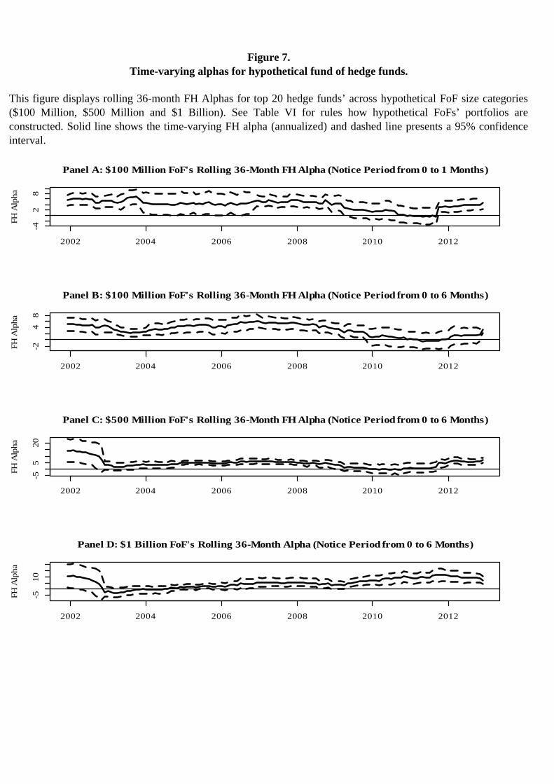
This figure displays rolling 36-month FH Alphas for top 20 hedge funds’ across hypothetical FoF size categories($100 Million, $500 Million and $1 Billion). See Table VI for rules how hypothetical FoFs’ portfolios areconstructed. Solid line shows the time-varying FH alpha (annualized) and dashed line presents a 95% confidenceinterval.
Time-varying alphas for hypothetical fund of hedge funds.Figure 7.
Panel A: $100 Million FoF's Rolling 36-Month FH Alpha (Notice Period from 0 to 1 Months)
FH A
lpha
2002 2004 2006 2008 2010 2012
-42
8
Panel B: $100 Million FoF's Rolling 36-Month FH Alpha (Notice Period from 0 to 6 Months)
FH A
lpha
2002 2004 2006 2008 2010 2012
-24
8
Panel C: $500 Million FoF's Rolling 36-Month FH Alpha (Notice Period from 0 to 6 Months)
FH A
lpha
2002 2004 2006 2008 2010 2012
-55
20
Panel D: $1 Billion FoF's Rolling 36-Month Alpha (Notice Period from 0 to 6 Months)
FH A
lpha
2002 2004 2006 2008 2010 2012
-510