the effect of local government policies on housing...

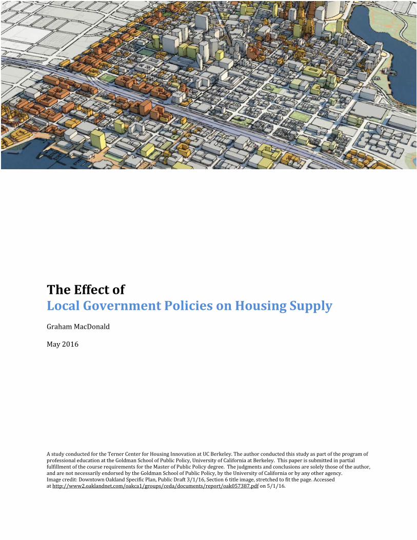
The Effect of Local Government Policies on Housing Supply Graham MacDonald May 2016 A study conducted for the Terner Center for Housing Innovation at UC Berkeley. The author conducted this study as part of the program of professional education at the Goldman School of Public Policy, University of California at Berkeley. This paper is submitted in partial fulfillment of the course requirements for the Master of Public Policy degree. The judgments and conclusions are solely those of the author, and are not necessarily endorsed by the Goldman School of Public Policy, by the University of California or by any other agency. Image credit: Downtown Oakland Specific Plan, Public Draft 3/1/16, Section 6 title image, stretched to fit the page. Accessed at http://www2.oaklandnet.com/oakca1/groups/ceda/documents/report/oak057387.pdf on 5/1/16.

http://www2.oaklandnet.com/oakca1/groups/ceda/documents/report/oak057387.pdf

The Effect of Local Government Policies on Housing Supply

2

Table of Contents Acknowledgements ............................................................................................................................................... 4

Executive Summary ............................................................................................................................................... 5

Housing Production is Important ................................................................................................................ 5

Summary of Recommendations .................................................................................................................. 5

Estimated Effects of Oakland’s Residential Impact Fee and Inclusionary Housing Policy .......................... 6

Estimated Effects of San Francisco’s Proposed Inclusionary Housing and Impact Fee Policy .................... 6

Brief Overview ........................................................................................................................................................ 8

Job Creation is Outpacing Housing Development ....................................................................................... 8

Rising Prices are Increasing Displacement and Can Slow Economic Growth .............................................. 8

Local Governments Make a Difference ....................................................................................................... 9

Project Goals ............................................................................................................................................... 9

Summary of the Literature .............................................................................................................................. 10

Additional Zoning Controls Increase Prices ............................................................................................... 10

Whether Zoning Controls Reduce Housing Supply Depends on Other City Actions ................................. 10

Feasibility Studies Can Help Policymakers Understand Developer Decisions .......................................... 11

Feasibility Studies May Miss Marginally Feasible Properties .................................................................... 11

Feasibility Studies Can Be Better ............................................................................................................... 12

Brief Summary of Methodology and Data .................................................................................................. 12

General Model of Project Feasibility ......................................................................................................... 12

Detailed Model for Parcels in Example Cities ........................................................................................... 13

Policy Alternatives ............................................................................................................................................. 13

Potential Options for Policymakers ........................................................................................................... 13

Criteria for Measuring Alternatives ........................................................................................................... 16

Findings and Discussion ................................................................................................................................... 16

General Model Findings ............................................................................................................................ 16

Example City Findings ................................................................................................................................ 21

Other Policy Considerations ...................................................................................................................... 24

Current or Recent Policy Proposals ............................................................................................................. 24

Estimated Effects of Oakland’s Residential Impact Fee and Inclusionary Housing Policy ........................ 24

Estimated Effects of San Francisco’s Proposed Inclusionary Housing and Impact Fee Policy .................. 25

Limitations ............................................................................................................................................................ 27


3

Appendix A: Methodology ................................................................................................................................ 29

General Model ........................................................................................................................................... 29

Example City Model .................................................................................................................................. 35

Appendix B: Data Sources ................................................................................................................................ 40

Appendix C: Complete Example City Results ............................................................................................. 41


4

Acknowledgements This paper would not be possible without the guidance, advice, and feedback of my client Carol Galante and advisor Dan Lindheim, to whom I owe a thousand thanks. I would also like to thank the incredibly kind city staffers, advocates, and development professionals who took the time to meet with me, answer questions, and provide feedback on my project – John Protopappas, Mike Ghielmetti, Bill Falik, Rick Holliday, Dennis Williams, John Stewart, Robert Freed, Denise Pinkston, Charles Gibson, Will Hu, Joe South, Jamie Choy, Jeff Levin, Sasha Hauswald, Eric Angstadt, Stephen Barton, Annie Campbell-Washington, Alex Marqusee, Adam Simons, Greg McConnell, Dan Schoenholz, Sarah Karlinsky, Thomas Gonzales, Robert Poole, Michael Lane, Ben Boyd, Steve Tipping, Sonja Trauss, Jed Kolko, Ted Egan, Sara Draper Zivetz, and others whose names I’ve missed. For their timely and fast assistance with data, I truly appreciate the help of Mike Wynne, Micaela Pronio, and Rusty Wynn.


5

Executive Summary Housing Production is Important From 2010 to 2015, there were 6 times as many new jobs and people as new housing units in the Bay Area, and home prices rose by 54% over this period. In the most recent year – 2015 – little has changed – 6 jobs and 4 new people were gained for every new housing unit, while home prices rose faster than in previous years1. To accommodate this growth, cities can change local policies to encourage housing production. In consultation with many developers, city planners, politicians, and advocacy groups, I created two models that summarize the relative impact different local policy measures have on housing production. I then weigh the models’ results against potential equity, administrative, and political concerns. The first model describes the effects on the odds that a given project will be built, while the second examines the cumulative impact on an entire city in four local jurisdictions. Examining the effect on every developable parcel in a city represents an improvement over existing feasibility models, which typically focus on a few example sites in a given city. And because many cities do not complete feasibility analyses, pay large sums of money to complete them, and/or produce long, complex reports, providing a transparent, open resource for policymakers can improve local decision making. Summary of Recommendations To increase housing production, my analysis indicates cities should pursue the following policies. Overall, the size of the impact on feasibility is highly dependent upon the strength of underlying market conditions and which policies a city already has in place.

1. Reduce ground floor retail requirements by up to 40%: This policy works best in marginally feasible project areas where retail rents are relatively weak, allowing developers to replace unprofitable retail with profitable residential space

2. Reduce parking requirements by 20%: This policy generally works best in marginally feasible areas with parking requirements of 1 space per unit or above, especially near public transit, allowing developers to replace unnecessary, expensive parking spots with profitable residential space

3. Eliminate costly conditional use requirements, and remove environmental review requirements through a specific plan: This policy works best in areas with conditional use requirements not covered by an area specific plan, as removing public environmental and local planning processes typically leads to significant savings. However, this can be expensive in the case of a lengthy specific plan process, and potentially politically unpopular because allowing permitting by right removes significant public input

4. Decrease basic permitting time for ministerial measures: Reducing time for design review, plan check, building permit approval, etc. may produce a range of effects, depending on a city’s current review time and the project size, largely because developers must provide significant annual returns to investors, who provide the capital. Places like San Francisco, with longer permitting timelines, may see larger benefits from this policy change

5. Increase density: This policy change only has a large effect in financially feasible areas with high rents, or in other areas zoned for less than 4 or 5 stories, and it may be politically challenging. However, in areas where a city has implemented a number of the previous recommendations, such as San Francisco, increasing density may be the best option

1 Author’s analysis of Bureau of Labor Statistics Current Employment Statistics, Census Bureau 2015 Population Estimates, and HUD SOCDS Building Permits Data.


6

Under current conditions, my analysis indicates that San Francisco should consider reducing permitting time and increasing density limits, while Oakland should consider modestly decreasing ground floor retail and parking requirements and reducing permitting time. In smaller cities like Pleasanton and Menlo Park with few developable properties, larger changes in zoning are necessary to significantly increase housing production and revenues. These recommendations consider only local government controlled factors affecting development, but other forces such as market rents, investor and developer target return, and construction costs may have far larger impacts on project feasibility. For a more complete understanding of how market forces and policy decisions interact, and to get an idea for what makes a project “marginal”, visit the interactive single project model at http://ternercenter2.berkeley.edu/proforma and the interactive citywide example cities model at http://ternercenter2.berkeley.edu/examplecities. Estimated Effects of Oakland’s Residential Impact Fee and Inclusionary Housing Policy The City of Oakland recently passed a policy on May 3rd, 2016, that, though much more nuanced, essentially requires 10% affordable housing at 120% of Area Median Income (AMI) or a fee of $24,000 per residential unit. The model estimates that, on average, this policy may reduce the city’s potential housing production – both market rate and affordable units combined – by 6-12%, or 354 to 569 potential units, reduce potential city property, fee, and transfer tax revenues by 5-12%, or $0.9 to $1.9 million per year, and increase potential affordable housing production from 4% of all housing units produced to 11%, an increase of 297 to 367 potential units, though these units would likely be at higher income levels than if the policy were not enacted. The model predicts that most developers would opt to build the affordable housing on site. The policy splits the city into three zones, phases in fees over time, and does not include many projects currently in development agreements in the city, so the actual effects are likely to be lower. Estimated Effects of San Francisco’s Proposed Inclusionary Housing and Impact Fee Policy The City and County of San Francisco is currently proposing, as of April 2016, to increase its on-site inclusionary requirement from 12% to 25%, with 15% going to renters at 55% of AMI and 10% to renters at 100% of AMI, or 15% to condo purchasers at 80% of AMI and 10% to condo purchasers at 120% of AMI. The current proposal will raise the fee from 20% of units to 33% of units, which I model as an increase to $115,000 per residential unit. The model estimates that, on average, this policy may reduce housing production by 4-17%, or 1,521-6,267 potential units, reduce potential city property, fee, and transfer tax revenues by 6-19%, about $9.2-$27.7 million per year, and increase potential production of affordable housing units from 13% of all housing units produced to 25-26%, an increase of 3,129-4,529 potential units, depending on how developers model the tradeoffs between rental and ownership units. Recent proposed legislation may grandfather many projects, however, and the analysis assumes that a state density bonus is not adopted, so the actual effects of the policy may differ. If the state density bonus law is adopted, these effects may be reduced by more than half. In both San Francisco and Oakland, the model estimates that these policies are likely to create more affordable units than could be created by dedicating the property tax revenue from lost production to affordable housing. However, due to the on-site requirements, many of the newly created units are likely to be at higher AMI levels than those that would be built by affordable housing developers.

http://ternercenter2.berkeley.edu/proforma

http://ternercenter2.berkeley.edu/examplecities


7

Blank Page


8

Brief Overview Job Creation is Outpacing Housing Development Employment and population in the San Francisco Bay Area2 are growing much faster than housing. From 2010 to 2015, the region grew by about 531,000 jobs3 and 487,000 people4, but only issued permits for 82,000 housing units5, a ratio of about 6 additional jobs and people per new housing unit. Plan Bay Area, the Bay Area’s current region-wide planning document, released in 2013, called for an increase of 1.1 million additional jobs, 2.1 million additional people, and 660,000 new housing units between 2010 and 20406. Five years into the plan’s life, rapid growth has ensured that the region has exceeded both the plan’s initial population growth projections by 100% and its initial job growth projections by 300%, though the region is on pace to meet the plan’s original housing goals. Even as the real estate market entered a “boom” in 2015, the jobs-housing balance has remained the same – the region continued to add 6 additional jobs per new housing unit, just as it had in the previous two years. The population-housing balance has declined slightly in recent years to just above 4 new people per housing unit by 2015, more than twice the ratio called for by the current regional plan. Rising Prices are Increasing Displacement and Can Slow Economic Growth When the number of new jobs and people exceeds the number of new housing units, prices generally increase, and people are forced to choose a combination of a longer commute and less disposable income, which, though bad in and of itself, can also slow economic growth. Between 2010 and 2015, rental rates and home sales prices increased by 45-55% on average, equivalent to annual increases of 8-9%7. Some of this rise represents a natural rebound from the Great Recession, in which a large portion of homeowners owed more than their homes were worth. By the end of 2013, however, the San Francisco and San Jose metro areas averaged less than 10% of homeowners with “negative equity”, one of the lowest levels in the nation and a drop of about 2/3 since 20118. Though most of the natural rebound had occurred, prices continued to rise between 2013 and 2015 by 21-25%, equivalent to annual increases of 10-12%. Rapidly rising prices – especially rents – have pushed low-income renters farther and farther from work – a recent Zillow study found that the average minimum-wage worker in San Francisco lived about 15 miles from work in 2013, compared to just 9 miles in 2010, a 67% increase in average commute distance over just 3 years9. Half of renter households pay more than 30% of their income on rent, a figure that has remained fairly steady from 2010 to 2014, the latest year in which data is available. Given the share of unrelated people living together has remained fairly steady over that time, the most likely explanation is that higher-income households are moving to lower-income communities close to work, forcing lower-income households farther and farther from job centers10.

2 Defined for the purposes of this paper as the 9-county region as defined by the Association for Bay Area Governments – Alameda, Contra Costa, Marin, Napa, San Francisco, Santa Clara, San Mateo, Solano, and Sonoma counties 3 Author’s analysis of Bureau of Labor Statistics Current Employment Statistics data 4 Author’s analysis of Census Bureau 2015 Population Estimates data 5 Author’s analysis of HUD SOCDS Building Permits data 6 Plan Bay Area 2013, Association of Bay Area Governments. http://planbayarea.org/the-plan/adopted-plan-bay-area-2013.html 7 Author’s analysis of Zillow Research ZHVI All Homes Time Series and ZRI Time Series: Multifamily, SFR, and Condo/Coop. http://www.zillow.com/research/data/ 8 Author’s analysis of Zillow Research Negative Equity Time Series. http://www.zillow.com/research/data/ 9 Zillow Research. http://www.zillow.com/research/seattle-san-fran-affordable-housing-11297/ 10 Author’s analysis of 2010 to 2014 American Community Survey data and Census Public Use Microdata Sample (PUMS), accessed via IPUMS USA.

http://planbayarea.org/the-plan/adopted-plan-bay-area-2013.html

http://www.zillow.com/research/data/

http://www.zillow.com/research/data/

http://www.zillow.com/research/seattle-san-fran-affordable-housing-11297/


9

High housing costs can slow economic growth by making it harder for businesses to recruit and retain employees. According to a 2014 survey of 222 CEOs and business executives in the Silicon Valley Leadership Group, business leaders’ top concern was “housing costs for employees”, followed by “employee recruitment/retention costs”, likely related to housing costs. At the local level, two of the top three recommendations business leaders made to policymakers in the area included easing traffic congestion and approving “more affordable home developments” 11. Local Governments Make a Difference In California, local governments have substantial control over the quantity and type of housing that can be built. Through the local zoning code, cities decide how much housing can theoretically be built, whether it can be built by right or requires significant public review, whether the developer needs to perform a costly environmental review, fees that a developer must pay, parking and retail required on site, and the design of the building, among other regulations. And these factors can be significant – a 2002 study by economists from Harvard and the University of Pennsylvania found strict zoning controls to be the most likely cause of high housing costs in California12. Project Goals This project has two primary goals. The first is to understand which local policies produce the most significant impacts on housing production in general. In other words, for a random development project, which local regulations have the biggest impact, both positive and negative? The second is to understand the impact of these policies in four local “example” jurisdictions, to understand how different local factors, such as rents and existing regulations, change the impact of the city’s local regulations on local housing development. Both models use local data to set reasonable defaults and measure the interaction between local public policies and the economic conditions of local Bay Area municipalities. The project is focused on residential housing production, and does not focus on retail, office, commercial, industrial, or any other real estate sector. The project focuses on retail only to understand the effects of ground floor retail requirements. Therefore, this project may not apply as well to cities considering legislation on commercial impact fees or mixed-use requirements. This project only considers policy changes within local governments’ control, and therefore may not apply to policymakers considering statewide policy changes and impacts. Many local governments in the Bay Area – including San Francisco, Oakland, Fremont, Berkeley, and others – are currently proposing or have recently proposed housing policies aimed at addressing the issues of affordability and displacement of lower-income households. Some of these policies – including inclusionary zoning and impact fees – may have an effect on housing production, and the goal of this paper is to help policymakers understand the relative size of these impacts. Other strategies that affect housing supply in less obvious ways – such as passing local housing bonds and instituting rent control – are outside the scope of this paper, though they may in certain cases be even more compelling policy options. Understanding the impact of local policies on housing supply is but one potential solution among many to address these pressing issues.

11 Silicon Valley CEO Survey. Silicon Valley Leadership Group. 2014. http://svlg.org/wp-content/uploads/2014/03/CEO_Survey_2014.pdf 12 Glaeser, Edward L., and Joseph Gyourko. The Impact of Zoning on Housing Affordability. Working paper no. 8835. National Bureau of Economic Research, Mar. 2002. Web. 24 Mar. 2016.

http://svlg.org/wp-content/uploads/2014/03/CEO_Survey_2014.pdf


10

Summary of the Literature Additional Zoning Controls Increase Prices The research on zoning controls, including impact fees and affordable housing requirements, indicates that increasing requirements increases housing prices. Glaeser and Gyourko, as previously mentioned, found that strict zoning policies were the primary driver of high housing costs in California13. A summary of the literature on impact fees conducted in 2008 found that impact fees lead to an increase in the cost of housing for both new and existing homes14. A summary of the literature on inclusionary zoning conducted in 2015 found that, in California, inclusionary zoning policies tended to increase housing prices by a small amount15. Though the literature generally agrees that increasing zoning controls leads to higher housing prices, researchers disagree on exactly how this happens. In their summary of the literature, Nelson et al. notes that scholars writing in the 1980s and 1990s argued that impact fees result in a decrease in the supply of housing, which leads to increased prices. More modern studies, however, argue that increased impact fees lead to increased local government spending, because many ordinances require governments use the impact fees on local infrastructure projects. These authors argue that this additional spending in turn increases the value of the neighborhood, and therefore it is increased spending, not necessarily decreased supply, that causes the observed price increases16. Been, in a 2005 piece, disagrees with the modern interpretation, arguing that a rising tide of demand in communities with impact fees causes prices to be bid up17. Whether Zoning Controls Reduce Housing Supply Depends on Other City Actions Much of the disagreement is a result of a lack of research on the effect of zoning controls on housing supply in the short run. As Nelson et al. and Hollingshead note in their literature reviews on impact fees and inclusionary housing, there are only a handful of studies addressing this issue, and they have found that these controls either increase, do nothing to, or decrease the housing supply. The reviewers explain this confusion by noting that municipalities may change other local development-related factors simultaneously that are not measured in the research, which may partially or fully negate the negative effects of the studied policies18. For example, if impact fees are introduced but this eliminates community opposition, increasing developer certainty and reducing development time, implementing impact fees could theoretically reduce development costs and increase housing supply. In the long run, as Hollingshead argues, most economists agree – housing supply is largely unaffected as any potential increased costs of local policies result in diminished land values19. Over time, landowners slowly begin to factor in the costs of local policies into decreased land prices, and land prices settle at a new, lower equilibrium in the market. Until landowners adjust to the new reality, developers may find it difficult to convince them to accept less money when comparable plots of land recently sold before the policy change received more.

13 Ibid. 14 Nelson, Arthur C., Liza K. Bowles, Julian C. Juergensmeyer, and James C. Nicholas. A Guide to Impact Fees and Housing Affordability. Washington, DC: Island, 2008. Print. 15 Hollingshead, Ann. When and How Should Cities Implement Inclusionary Housing Policies. Rep. Cornerstone Partnership, May 2015. Web. 25 Mar. 2016. 16 Ibid. 14 17 Been, Vicki. "Impact Fees and Housing Affordability." Cityscape 8.1 (2005): 139-85. Department of Housing and Urban Development. Web. 25 Mar. 2016. 18 Ibid. 14 & 15 19 Ibid. 15


11

Feasibility Studies Can Help Policymakers Understand Developer Decisions This project aims to measure how developers in Bay Area cities might react to changes in local policies. Since the literature is unclear on how these policies affect housing supply, it is important to understand how economic consultants currently model development feasibility in Bay Area cities in order to more accurately model the effects of local policies. Based on conversations with local Bay Area Planning Department staff, it is clear that most city Planning Departments put together a static pro forma – some simple, and others more complex – when contemplating significant zoning changes, though not all cities do a formal feasibility analysis. A static pro forma models the costs and potential returns to a single development on a plot of land at a single point in time. The pro forma provides the expected profit the developer might receive and the amount she can afford to pay for the land. In some cases, cities contract with economic consultants to do a more rigorous static pro forma analysis called a feasibility study. In the Bay Area, I collected 5 different feasibility studies conducted over the past 4 years in 3 different cities – San Francisco, Oakland, and El Cerrito – in order to understand how cities and their consultants model future development decisions. In general, the reports follow fairly similar methodologies, which involve choosing a few example sites and construction typologies representative of likely development in a few key areas of each city, gathering detailed local market data – such as local costs, rents, and zoning restrictions – and running a static pro forma analysis to determine the profitability of the project. For example, a city might study the feasibility of a single family, townhome, and low-rise apartment building in 5 different vacant parcels spread throughout the city, where there might be significantly different rents, in order to test their assumptions. Most reports use a Residual Land Value (RLV) approach to determining project feasibility. The RLV method takes into account all of the necessary costs to build a project – with the exception of the value of the land – specifies a required investor and developer return, and then calculates the maximum the developer would pay for the land to make her target profit. When this amount approaches or exceeds the current market price of land, the consultant determines that the project is likely financially feasible. Feasibility Studies May Miss Marginally Feasible Properties Most feasibility studies in the Bay Area use a few example sites to study the effects of policy changes on residential development feasibility. As a result, these studies measure feasibility for a few prototypes, but do not tell policymakers how common those prototypes are throughout the city. For example, a feasibility study may look at a typical 5 story residential complex on vacant land in north Oakland, and will report whether the development will be financially feasible under a number of different fee and affordable housing requirements. However, the study will not say how many plots of land are vacant, zoned for 5 stories of residential, and can achieve the market rents assumed for that area. If there are a large number of properties with these characteristics, the study may be fairly accurate, but if there are only a few, the study may not be of much use in generalizing to the local area. Even if the examples chosen are relatively representative – for example, the example site chosen represents 70% of the properties in the given area – it may fail to measure the effect of policy changes on the remaining 30% of properties. If many of the properties not represented by the example are marginally feasible – that is, they are highly susceptible to small changes in development


12

assumptions and market forces – small changes in public policy could make a large difference in project feasibility. Failing to consider the properties that don’t conform to the example site selected may prevent policymakers from making a fully informed decision on the impact of policy on local development. By considering all developable properties in a jurisdiction, a more complete model can better predict the impact of a policy decision on development potential. Feasibility Studies Can Be Better Even when jurisdictions do complete a feasibility analysis, these studies can be quite expensive, end up taking the form of long, complex reports and tables, and fail to report the overall effect of the policy on the city as a whole. For example, to perform a nexus and feasibility study, the City of Oakland recently authorized $1.1 million for a consultant, Hausrath Economics Group, to complete a report.20 However, when considering the impact fee, the city attached to the legislation only a summary and presentation of the consultant’s work, which provided recommendations, detailed tables and comments. Though the report did a thorough job examining the impact of a fee on a few example developments, it contained little explanation of the methodology beyond the tables and did not attempt to measure the magnitude of the policy’s impact on total housing production and revenues. Improving the way cities conduct feasibility analysis by providing transparent, easy to use, open tools that can be used by jurisdictions can ensure that:

1. Policymakers understand the impacts of their decisions 2. The public can have improved access to accurate information 3. All parties understand the model’s assumptions and can judge potential tradeoffs.

Brief Summary of Methodology and Data General Model of Project Feasibility The first goal of this project is to help policymakers understand, for a given project, the most important policies, and other factors, influencing the odds of whether the project gets built. The project focuses on the effect over a 5 to 10 year period to focus on short- to medium-run effects. To develop a sound general development model, I combined evidence from the literature, feasibility studies, and interviews with development professionals to create a complex, dynamic21 pro forma model. The model focuses on the most important factors to development and produces a probability that the project will be built, ranging from 0 to 99%. As such, the model allows many key assumptions to be changed and provides a transparent gauge of a project’s sensitivity to any changes to these important assumptions. The project uses a RLV approach, described in the previous section, in order to come up with the maximum value a developer might be willing to pay for the project given the model’s inputs – local market factors, zoning constraints, and required investor and developer return. The model then divides this value by the market rate value of land, also an input, to get the value of the land to a housing developer relative to the current value of land in the area. Because some land owners are financially motivated – say, some are in serious financial trouble and need to sell – while others can afford to hold the land for a long period of time, I assume that as the

20 https://oakland.legistar.com/View.ashx?M=F&ID=3383019&GUID=A295E91C-67C9-4AA2-852C-D9226F923B67. Though the city does not specify how much is paid for the nexus study and the feasibility study separately, it is likely that the study cost 10s to 100s of thousands of dollars. 21 Here, I still use a static pro forma that does not use a discounted cash flow analysis to calculate project value, in which the pro forma uses assumptions from a single point in time. The pro forma is dynamic in the sense that I allow many of the assumptions to be changed, and study the effects of the changes in these assumptions on project financial feasibility.

https://oakland.legistar.com/View.ashx?M=F&ID=3383019&GUID=A295E91C-67C9-4AA2-852C-D9226F923B67


13

price of the land relative to market price increases, more and more land owners will be willing to sell. I also assume that at a certain price, twice that of the market rate value of land, all land owners will be willing to sell. If the land owner is willing to sell, the project gets built. The share of land owners in the market area that might be willing to sell is then the probability the project gets built – the probability represents the odds that a project is sitting on land owned by a willing landowner at the price the developer can afford to pay. This probability is important for calculating total development potential in an area, which I discuss in the detailed model methodology below. Total development potential may not match actual development in the short term, as developers may seek the most motivated landowners first. For a complete discussion of the general model Methodology, see Appendix A: Methodology. Detailed Model for Parcels in Example Cities The second goal of the project is to understand how the importance of the factors in the general development model change when put in context in four example cities – San Francisco, Oakland, Pleasanton, and Menlo Park. The model uses parcel-level data from cities and counties, including manually collected zoning information, local market rents and sales prices within a quarter-mile of each parcel, and information on liquefaction and landslide zones, and narrows the city’s parcels down to those that are built out to 20% or less of their development potential, according to the zoning code. The general development model is applied to each parcel to determine the probability that a housing project will be built. These probabilities are reduced the longer the landowner has owned the parcel, if the landowner is a public entity, and if the current value of the existing use on the parcel is greater than the value the developer is willing to pay for the land. The model does not consider any re-zoning to different uses, focusing only on parcels currently zoned by right or conditional use for residential development. Once the calculations are complete, the model can calculate the range of total development and city revenue potential, in a rough 10th percentile to 90th percentile range based on a Monte Carlo simulation of potential outcomes – using a simulated Monte Carlo approach allows me to report a confidence interval. When calculating revenue potential, the model calculates only the city’s share of the local property tax received. For a complete discussion of the example model Methodology, see Appendix A: Methodology.

Policy Alternatives Potential Options for Policymakers Policymakers can choose among a number of policy tools that can have a significant impact on housing production in their jurisdiction. I limit the alternatives to the following policies in order to provide a short list of the most effective policy tools, identified from conversations with policymakers, city staff, and development experts. Conditional Use Permits and Planned Unit Developments: A Conditional Use (CU) permit and Planned Unit Development (PUD) permit are zoning designations created by cities that require a developer to get approvals from the local Planning Commission and possibly City Council in order to go through with development. These designations are usually included in order to ensure a process by which local concerns can be resolved with individual proposed developments.


14

For example, bars are often conditionally permitted, in order for neighbors to have input into the bar’s hours, level of outside music, parking, and other potentially disrupting factors. In some instances, with little community and City Council opposition, this process may be relatively quick and costless. In others, with strong community turnout and pressure on the City Council, this process can significantly lengthen the development process and add large costs. Deliberations between different interests may take significant time to resolve, at the cost of city staff time and the carrying cost of the developer’s investment in land, architects, engineer, and staff time. Specific Plan Areas: A specific plan is a development plan created by the city to encompass an area, usually comprising a few neighborhoods representing a subset of the city, with new zoning rules and requirements. As part of the Specific Plan, the city completes an Environmental Impact Report (EIR) for the specified area, with necessary mitigations, and as a result, developers requiring discretionary project approval do not have to complete the environmental review process within the Specific Plan area as long as they comply with the mitigations set forth in the plan. Discretionary project approval usually involves some sort of approval from the local Planning Commission or City Council, usually accomplished through a CU or PUD, and excludes things like Design Review and building permit applications. Based on interviews with Bay Area developers, the EIR process can take 12 to 24 months and can cost an extra $300,000 to upwards of $1 million, depending on the size of the project. If the project is sued under the California Environmental Quality Act, additional time and cost delays are possible. As a result, Specific Plans can help lower the cost of projects needing discretionary review in Specific Plan areas significantly. Inclusionary Zoning: Cites may require that a certain percentage of the units in a new development be made affordable, for a certain period of time, to people earning certain incomes, as specified by the city. In California, recent court decisions have spurred localities to allow developers to choose to pay a fee or build affordable housing on site. So, for example, if a city sets their Affordable Housing requirement at 10% and their fees at $0, developers will choose not to build the affordable housing and will instead choose to pay a $0 fee. Both controls must be changed in order to change developer incentives. Finding the correct balance between the two, so that a developer is indifferent between building affordable units and paying the fee, is difficult. Depending on the levels set, the bonus in density the developer receives from the locality for building affordable housing, and the income levels required for affordable housing, this requirement can mean the difference between a developer building the project or walking away. Impact Fee: Cities may charge a certain amount per unit, or per square foot, for new residential construction. In California, recent court decisions have spurred localities to allow developers to choose to pay a fee or build affordable housing on site. See Inclusionary Zoning, above for a brief explanation of this process. All other impact fees, such as sewer and water fees, are not included in this definition, and are included in a general “soft cost” figure in the model. Density: Cities have various options for restricting the amount of residential space built on individual properties. Some cities restrict based on the number of units: maximum number of units, dwelling units per acre, maximum number of units per square foot of property, maximum height. Others restrict based on the size of the space: minimum lot area, maximum ratio of floor area to square feet of property. And many do both. Cities may change the density in any area by establishing new zoning restrictions or changing or eliminating existing ones.


15

Changing density restrictions does not necessarily result in increased or reduced production. Because of building codes, building higher than 6 stories involves more costly construction materials and often labor, and depending on the lot size, certain building heights may not be economically feasible. In general, increasing density is most effective in areas with high economic feasibility – where the general model determines the project is able to pay a significant premium above market land values, due to high rents, low costs, or a combination of the two. Parking Requirements: Cities typically regulate parking by requiring a certain number of parking spaces per new unit constructed. A typical requirement for single family homes is 2 parking spaces per unit, while for center city properties, the requirement may range from no parking to 1 space per unit. Parking can be quite expensive because most parking structures for low-rise units are built of podium – Type I construction22 – and parking spaces require not only the space needed for the car but also extra space for that car to back out and leave the garage. Depending on the type of construction and technology used, parking can range from $30,000 per space to $75,000 per space. Given that developers are currently building units for $450,000 to $500,000 per unit, parking can represent anywhere from 3% to 17% of costs. In many cases, space not used for parking may be used to construct additional residential units, increasing project feasibility. Therefore reducing parking requirements in areas where parking is not required at current levels, even by modest amounts, can significantly affect project costs. Ground Floor Retail Requirements: In areas planned for high retail traffic, cities typically require that there be space set aside on the ground floor for retail space. Some cities specify ground floor retail only along certain corridors, while others require it be situated throughout the entire ground floor. Ground floor retail typically requires ceilings of 15 to 17 feet, much higher than the typical 9 to 10 foot requirement for residential housing, and lots of glass fronting major thoroughfares, requiring higher cost construction materials and labor. In areas where retail traffic and rents are high, these requirements may not adversely impact new development. However, in areas where retail rents are significantly below residential rents, and the planned foot or vehicle traffic has yet to arrive, these requirements can significantly affect project costs. Without major “credit” tenants – for example, CVS or Subway – committed to the space, banks are unlikely to lend to developers building in these nascent retail areas. Without existing foot or vehicle traffic, it may be difficult to convince major retailers to take a chance on future development. Space set aside for ground floor retail could otherwise be used for parking, common area space, or residential living space. Permitting Time: Permitting time is defined here as all ministerial actions necessary for project approval, including design review, plan check, and building permit application approval. Not included here are reviews by the Planning Commission and City Council. Though not directly regulated in the local municipal code, permitting time is indirectly regulated through the number of staff allocated to completing plan checks, doing design review, taking time to work with a developer through the process, the availability of Planning Commission time slots, and building permit processing. The more staff the city allocates to the process, the cheaper development becomes. This is especially true in areas with significant backlogs, where projects can be held up by months before a planner is even assigned to begin the project review, before design review even

22 A typical low-rise residential building consists of a concrete “slab” on the ground floor (Type I) for parking and/or retail space and 4-5 stories of wood-framed residential space above


16

begins. Some areas have expedited processes, in which many of these functions may be completed quickly, for a fee. Some developers may also hire consultants – some of whom are previous government employees – to achieve the same goal. Time is money to developers because contracts are specified with major investors – such as pension funds – to deliver a guaranteed annual return. If a developer is required to return 12% per year to a pension fund on a project in which the fund has invested $10 million upfront in plans, land, and other consulting costs, a one year delay can mean an additional $1.7 million in project costs when the project is finally built 3 years later as the cost is compounded over time. Criteria for Measuring Alternatives The primary purpose of this report is to measure the impact of each of the policy alternatives, however cities must also consider equity, political feasibility, and administrative costs when implementing public policies. For example, in a number of Bay Area locations, especially those closest to downtown San Francisco, displacement of low-income families to locations farther from the city is a pressing equity concern and a top political issue. To determine which policies are most likely to be enacted, supported, administratively cheap, fair to all citizens, and effective, I rank the policy alternatives using a weighted sum of impact, equity, political feasibility, and administrative cost. For the purposes of this analysis, I consider impact, political and administrative feasibility, and equity equally. Each criterion, with the exception of impact, is rated on a 5-point scale from low to high, with low being bad and high good. Impact is measured on a continuous scale to give policymakers an understanding of the relative sizes of each of the policies.

Findings and Discussion In the following two sections, I define “marginal housing developments”, “marginal projects”, and “marginally financially feasible projects” as those developments – as indicated by the model – whose probability of land sale and construction is significantly affected by small changes in any of the models’ inputs. Whether a project is marginally feasible depends on a number of interrelated factors. Practitioners seeking to understand whether a project or projects in an area are feasible can use the interactive general model tool, at http://ternercenter2.berkeley.edu/proforma. General Model Findings The headings for the table below are defined as follows: Effect: Under some circumstances, projects may be highly feasible or infeasible, and so a change may have no effect, while for marginal projects, a change may have a large effect Equity: To what extent does the project affect different groups of people differently? Politics & Admin: How politically popular is the project, and how low are the administrative costs to implement it? Overall Rating: Weighted average of the three considerations. Policy Effect Equity Politics & Admin. Overall Rating Reduce Ground Floor Retail Requirement 40%

0-99% High Moderate High-Moderate

Parking Reduced 20% 0-87% High Moderate High-Moderate Specific Plan 0-94% High-Moderate Low-Moderate High-Moderate Permitting Time Reduced 33% 0-86% High Moderate High-Moderate Conditional Use Eliminated 0-99% Moderate Low-Moderate Moderate



17

Density Increased 25% 0-26% High-Moderate Low-Moderate Moderate Reduce Inclusionary 50% (from 20% to 10%, for example)

0-99% Low Low Low-Moderate

Impact Fee Reduced 50% (from $40,000/unit to $20,000, for example)

0-98% Low Low Low-Moderate

In general, reducing ground floor retail requirements, reducing parking requirements, eliminating conditional use requirements, and implementing specific plans are the most promising policies that cities can take to increase development potential. Each comes with potential caveats that depend heavily on existing regulations and market conditions in a city, which I explain below. This section details the results of potential local government policy changes. Typically market forces such as investor and developer target return (and perceived risk), local sales prices and rents, and construction costs will have a much larger effect than the policy changes listed here. What may be a marginal project in one year may be feasible in a time of rising rents or infeasible during a recession. For a more complete understanding of how market forces and policy decisions interact, visit the interactive general model at http://ternercenter2.berkeley.edu/proforma. For all of the impacts detailed in this section, I write “0% to x%” to specify the maximum possible effect, x, and describe the conditions necessary for that effect to occur. Under certain conditions, however, each policy lever may not change the probability of development at all. For example, projects in extremely low-rent areas may be so far from financial feasibility that no policy action short of a direct subsidy could promote development. Reduce Ground Floor Retail Requirement 40%: Reducing the ground floor retail requirement from 100% of the ground floor to 60% can improve the probability of development for a given project from 0% to 99%. To produce the maximum effect, the project must be marginally financially feasible, have a significant ground floor retail requirement (at least 40% of ground floor space), and retail rents must be significantly below residential rents in the area. If retail rents are high, or the project is already developable, reducing the requirement will make no difference. If retail rents are low, reducing the requirement means significant additional income from residential rents, which may cause the project to become financially feasible. Many cities require ground floor retail, but usually along specific corridors, and not all ground floor space may be required for retail. For example, two of the example cities in this study, Pleasanton and Menlo Park, have no ground floor retail requirement on any vacant and underdeveloped residential parcels. Oakland and San Francisco, on the other hand, have a large number of properties with significant ground floor retail requirements. Reducing ground floor retail may not produce significant equity concerns. It provides more housing units and is unlikely to result in the loss of small, low-income, or minority businesses, which would be unlikely to afford the rents of new ground floor retail spaces. Politically, the policy may satisfy the intent of planners and community members for active, ground floor uses and a vibrant commercial corridor, though there is likely to be some opposition. Administratively, measuring the amount of ground floor retail space is easily accomplished upon the city’s issuance of the certificate of occupancy.



18

Reduce Parking Requirement 20%: Reducing the parking requirement by 20 percent – for example, from 1 space per unit to 0.8 spaces per unit - can improve the probability of development for a given project from 0% to 87%. To produce the maximum effect, the project must be very close to being developable – a marginally developable property, where rents are almost high enough to justify construction. The project must have a significant parking requirement – for example, it must require at least some parking, and usually a significant amount of at least 1 space per unit, because a 20% decrease is much smaller when the original parking requirement is 0.25 to 1. And the effect on the project increases with the number of units in the project – reducing parking ratio required for 500 units makes a much larger difference than for a 10 unit project. Reducing parking not only removes parking cost but may allow for increased revenue through the addition of residential units or space per residential unit. Although a developer is unlikely to put a single unit on a ground floor built solely for parking, some developers place parking along the back of the complex and residential space, or common area access space such as a lobby, mail room, or manager’s office, along the front. Reducing parking may not produce significant equity concerns, though this depends on the location and project tenure. In walk-able urban corridors with strong public transit in rental properties, reducing parking marginally provides more housing units without significant effects on parking availability. In for-sale suburban areas without strong public transit access, reducing parking may increase congestion and face pushback from developers and homeowners. The administrative burden of measuring parking requirements remains unchanged. Politically, however, this issue may prove difficult in certain neighborhoods – residents may be afraid that reducing parking will lead to congestion and parking undersupply. These political concerns may be somewhat ameliorated by targeting the parking reduction to transit-friendly neighborhoods with low vehicle demand, or in areas with few existing residents. Specific Plan Areas: Creating a Specific Plan in one area can increase the odds that a project gets developed from 0% to 94%. To produce the maximum effect, the project must be a marginally feasible project and must be a large project, with at least a few hundred units. Development experts agreed that larger project were more likely to need to produce longer and more expensive environmental reports, and may also be more likely to attract expensive litigation. Specific Plans remove the requirement to do a full Environmental Review under the California Environmental Quality Act (CEQA) for all projects that require a CU, PUD, or other discretionary action. An Environmental Impact Report (EIR) may take over a year and can cost upwards of $1 million, depending on the project’s size and potential litigation. Specific Plans require extensive community input, which tends to mitigate many concerns over equity. However, Planning Department funds are finite, and many people who might not care enough to take time out of a busy day may not attend public meetings to shape the plan, leaving many low-income residents disproportionately affected by any changes. Politically, public input may lead to support for the Specific Plan, especially given the additional amenities promised to local residents, to be paid for through future fees on development.


19

Administratively, Specific Plans are usually expensive and time consuming. They must be initiated by the local Planning Department, and require the completion of an EIR by the city, the costs of which the city may attempt to at least partially pass on to developers. Specific Plans may involve extensive community input and therefore Planning Department staff time. In return, developers receive certainty, and often properties in the specific plan may be zoned by right. The lack of CUs or PUDs can provide significant development savings, as described in the previous section. Reducing Permitting Time: Again, permitting time is defined here as all ministerial actions necessary for project approval, including design review, plan check, and building permit application approval. Not included here are reviews by the Planning Commission and City Council. Reducing the amount of time necessary for ministerial actions such as design review and building permit applications by 33% – for example, from 6 to 4 months – can increase the odds that a project gets developed from 0% to 86%. To produce the maximum effect, the project must be a marginally feasible project. The project must also either have a long existing ministerial process – much longer than 6 months – or must be a large project with higher than average capital costs. Reducing development time reduces the amount that a developer must eventually return to an investor who requires an annual return, which is common in the real estate industry. Every additional month means the investor in the project must receive additional return, compounded on the amount invested, based on the annual rate. A decrease in time for purely ministerial actions that are part of a previous publicly approved process produces few equity concerns. Politically, this policy may do little to damage any group, and may face little opposition, though increased funding may cause some concern in cities struggling financially. Administratively, this is likely to involve additional staffing, coordination, and a change of processes, which may prove difficult, depending on budgeting constraints. Eliminating Conditional Use or Planned Unit Development Requirements: Eliminating the CU or PUD requirement for a project can turn a financially infeasible project with a 0% chance of development to a project with a 99% chance of development. To produce the maximum effect, the project must be very close to being developable – a marginally feasible project – or the costs and time of a CU or PUD permit must be high. If the additional cost and time required are high, the project need not be marginally feasible to produce the maximum effect. Eliminating CUs or PUDs can in some cases cause significant equity concerns. Traditionally, CUs and PUDs are used in order to deal unforeseen issues that a new use of the property may cause. Issues such as parking, types of housing allowed, the amount of affordable housing required, and others may be ignored or unaccounted for if Planning Commission and City Council discretion is eliminated. For example, if a large housing development sites its garage entry across the street from the entrance to a major commercial center, a city may want to require the developer move the parking entrance to avoid major traffic congestion. Without the CU or PUD process, the city may not have the power to compel the developer to make this change. But eliminating CUs and PUDs may also have positive equity effects. These processes may draw surrounding neighbors interested in reducing development to protect local property values. In this case, eliminating the requirement may allow for a more equitable distribution of housing units at different sizes and costs.


20

For these same reasons, this issue is politically difficult – many residents may not appreciate that they have no opportunity to block or negotiate changes project, though the process will likely be administratively simpler. For example, residents living around the major complex would likely want to negotiate a change in the parking entrance, but would not have the opportunity. At the same time, the city would not have to spend money putting together staff reports for commission meetings and mediating the dispute between neighbors and the developer. If CUs and PUDs are eliminated in the same process as a Specific Plan, however, the community may feel they have sufficient input into the process, and many of these issues may be avoided. In a Specific Plan process, which often lasts years, the public has a number of opportunities, through community meetings and Planning Commission and City Council meetings, to voice their concerns. Issues with the Specific Plan process are discussed below. Increasing Density: Increasing density limits by 25% – for example, moving height limits from 4 stories to 5 stories – can increase the odds that a project gets developed from 0% to 26%. To produce the maximum effect, the project must be financially feasible or marginally financially feasible, and the current height limit must not be at a threshold, defined by building code, that might make additional units cost significantly more money to build. For example, moving from a six story to a seven story building generally requires significant expense, because developers are forced by building code to build using more expensive materials and construction labor. Increasing density for the most cost effective types of construction – usually low-rise, 5 to 6 story buildings – to their maximum potential under code produces the largest effect. For example, cities with financially feasible residential areas zoned for 2 to 3 stories in height could benefit from up-zoning these areas to 5 to 6 stories. Because the construction typology is similar at both heights, developers can add units without significantly increasing the construction cost per unit. On the other hand, cities like San Francisco, with very high rents in the residential areas surrounding the Financial District, can benefit from up-zonings at most height levels without significant concerns for the increasing costs of construction per unit. Increasing density can cause some equity concerns, especially among the surrounding neighbors, though it is likely that outside observers would consider a 25% increase in density fairly modest. This, of course, depends on how the density increase is implemented and how neighbors are affected by the development. Allowing more units prioritizes new residents over existing residents, who may see increased density as a cause of potential traffic and parking issues in nearby streets, potential overcrowding of local public facilities, and increased noise and pollution unless these issues are remediated by the developer. For these same reasons, increasing density may be politically difficult. Administratively, increasing density can involve some challenges, as many competing factors often constrain development in an area. Depending on the size of the development and units proposed within the development, a few different zoning regulations might be the cause of current limitations to increased development capacity, and sorting through which ones will affect which developments may take a significant investment in staff time. Reducing Inclusionary Requirements: Reducing inclusionary requirements by 50% – for example, from 20% of units to 10% – can increase the odds that a project gets developed from 0% to 99%. Increasing inclusionary requirements by 100%, from 10% to 20%, would have the opposite effect. To produce the maximum effect, the project must be very close to being developable – a marginally feasible project – and the impact fees must be high enough so that the project chooses to build


21

affordable units on site both before and after the change to the requirement. The project must also require inclusionary housing at relatively low levels – for example, 50% of AMI – to produce a large effect. Reducing the inclusionary requirement increases the amount of income the developer can receive for the project, which makes a project more likely to be built. Reducing the inclusionary requirement may carry significant equity concerns. Low-income renters, especially those earning 30% or less of Area Median Income, often struggle to afford a place to live because the cost to maintain a quality rental unit, even in the cheapest parts of the Bay Area, is greater than the rent the landlord might receive. Producing less housing for lower-income people would only exacerbate these trends. However, even the most aggressive inclusionary programs rarely require such deep subsidies – most require apartments to be affordable to families earning 50-60% of AMI or above. Though this it is administratively simple to lower the level of the requirement, given current concerns over gentrification and displacement, this policy may be very politically unpopular, and would likely produce fewer affordable units overall. Reducing Impact Fees: Reducing impact fees by 50% – for example, from $40,000 per new unit built to $20,000 – can increase the odds that a project gets developed from 0% to 99%. To produce the maximum effect, the project must be very close to being developable – a marginally feasible project – and the affordable housing requirement must be high enough so that the project chooses to pay the impact fees both before and after the change to the requirement. Reducing impact fees directly reduces the cost of the project and therefore increases the chances that the project is developed. Reducing the impact fee requirement carries significant equity concerns, especially as some jurisdictions have required most of these revenues to flow to affordable housing. As argued in the previous section, low-income and lower-middle class households are disproportionately affected by this policy. In the case where the fees go toward parks, streets, city general funds, and other uses, reducing these fees may affect city residents more equally. Though this it is administratively simple to lower the fee levels, given current concerns over gentrification and displacement, and the budget struggles many California cities face, this policy would be very politically unpopular. Example City Findings The table measures the percentage change in potential housing units and city revenue, from the base case of current city policy, over the following 5 to 10 years. Increases Potential Production (& Revenue) in … Policy San Francisco** Oakland Pleasanton* Menlo Park* Specific Plans Citywide 4% (4%) 15% (7%) 62% (29%) 39% (50%) Conditional Use Eliminated 6% (5%) 15% (7%) 95% (61%) 290% (279%) Reduce Inclusionary 50% 16% (10%) 5% (1%) -3% (-6%) 0% (0%) Impact Fee Reduced 50% 7% (90%) 1% (9%) 15% (-3%) 0% (0%) Density Increased 20% 9% (10%) 5% (6%) 33% (23%) 31% (54%) Parking Reduced 20% 1% (2%) 19% (17%) 65% (41%) 286% (283%) Reduce Ground Floor Retail Requirement 40%

4% (3%) 30% (20%) 0% (0%) 0% (0%)

Permitting Time Reduced 33% 19% (16%) 18% (12%) 15% (3%) 14% (25%) *Results may be less reliable as these cities have very few developable properties within the size range in which the model is most accurate ** Yerba Buena and Treasure Island are not included because data were not available for this analysis The most effective policies for a city vary depending on local constraints and market factors, which I discuss below. Because Menlo Park and Pleasanton have so few properties that have not been


22

developed to at least 20% of their development potential, the results in these cities are less accurate and difficult to interpret, and I talk about them more generally in the discussion below. To reiterate, this section details the results of potential local government policy changes. Typically market forces such as investor and developer target return (and perceived risk), local sales prices and rents, and construction costs will have a much larger effect than the policy changes listed here. What may be a marginal project in one year may be feasible in a time of rising rents or infeasible during a recession. For a more complete understanding of how market forces and policy decisions interact, visit the interactive example model at http://ternercenter2.berkeley.edu/examplecities. In San Francisco, Increases Potential … Policy Housing Units Revenue Aff. Housing Units Base N = 33,672 to 39,197 $1.13 to $1.35 B 4,107 to 4,802 Specific Plans Citywide 2% to 6% 2% to 5% 1% to 6% Conditional Use Eliminated 5% to 7% 5% to 6% 3% to 7% Reduce Inclusionary 50% 15% to 17% 8% to 13% -38% to -35% Impact Fee Reduced 50% 6% to 8% 85% to 95% -77% to -74% Density Increased 20% 8% to 9% 9% to 10% 8% to 9% Parking Reduced 20% 0% to 2% 1% to 2% 0% to 3% Reduce Ground Floor Retail Requirement 40%

3% to 6% 3% to 4% 2% to 5%

Permitting Time Reduced 33% 17% to 21% 14% to 17% 16% to 22% San Francisco: In San Francisco, with high rents and a number of Specific Plan areas covering dense zones of the city, many areas with development potential are financially feasible. San Francisco has been a leader in removing parking requirements and in many neighborhoods has set parking maximums instead of minimums. Though the city does require ground floor retail on a number of key corridors, most of these corridors have high rents and do not adversely affect the financial feasibility of most projects. With an impact fee set at a slightly more expensive level than building affordable housing on site, the most effective factors to increasing development include reducing the inclusionary zoning requirement, reducing what developers report to be a long basic permitting process, and increasing density. Increasing density moderately could produce approximately 3,200 new units for the city and increase city revenue by $110 to $125 million in net present value over 10 years, or about $13 to $15 million per year. Reducing basic permitting time by 33%, or about 6 months in this case, could produce approximately 6,500 to 7,000 new units for the city, and increase city revenue by $190 to $195 million in net present value over 10 years, or about $18 to $24 million per year. Reducing the inclusionary requirement by 50%, or from 12% to 6% at 55% of AMI, could produce approximately 6,000 new units for the city, and increase city revenue by $100 to $150 million in net present value over 10 years, or about $12 to $18 million per year. Reducing the affordability requirement would decrease development expenses, reducing permitting time would reduce developer carrying costs, and increasing density in areas that are already financially feasible would further increase housing production and revenues. The model indicates that reducing the impact fee may incentivize developers to switch to paying the fee, as opposed to choosing to build affordable housing. A shift to more developers paying the fee would dramatically



23

increase revenue (while decreasing on-site affordable housing production), without significantly changing development potential. In Oakland, Increases Potential … Policy Housing Units Revenue Aff. Housing Units Base N = 4,588 to 5,472 $135 to $156 M 488 to 599 Specific Plans Citywide 13% to 17% 4% to 11% 16% to 16% Conditional Use Eliminated 13% to 17% 4% to 11% 16% to 17% Reduce Inclusionary 50% 5% to 6% 1% to 2% -22% to -18% Impact Fee Reduced 50% 1% to 2% 7% to 12% -15% to -10% Density Increased 20% 4% to 6% 6% to 6% 2% to 3% Parking Reduced 20% 18% to 20% 15% to 18% 18% to 18% Reduce Ground Floor Retail Requirement 40%

30% to 30% 19% to 21% 29% to 34%

Permitting Time Reduced 33% 18% to 19% 12% to 12% 17% to 25% Oakland: In Oakland, the model indicates that there are many marginally developable properties and many areas of the city where development is currently financially infeasible. Many of the places with feasible development – such as those in north Oakland and downtown Oakland – have significant parking requirements of at least 1 space per unit. In many of these spaces, the model finds that ground floor retail rents may be impediments to financial feasibility for marginal housing developments, depending on local retail rents. The most effective factors in Oakland, from the table above, align with the recommended factors from the general model. The model indicates that modestly decreasing ground floor retail and parking requirements, and permitting time may significantly impact many of the city’s marginal development projects and increase city revenue from property taxes. Reducing ground floor retail requirements would increase housing production by 1,300 to 1,600 units, and increase city revenue by $25 to $33 million in net present value over 10 years, or $3 to $3.9 million per year. Either reducing parking requirements or reducing permitting time moderately could produce approximately 800 to 1,100 new units for the city, and increase city revenue by $16 to $28 million in net present value over 10 years, or about $1.9 to $3.3 million per year. The magnitude and direction of the impact of reductions to inclusionary requirements and impact fees is similar to the general model’s findings of moderate, positive effects on potential housing production. In addition, reductions in permitting time and efforts to continue to expand the areas of the city covered by specific plans may create comparably large improvements in residential production and revenue. The model’s findings indicate that changes to further increase inclusionary zoning and impact fee requirements should be offset by changes in parking and ground floor retail requirements, permitting time, and the implementation of current and future specific plans to ensure development is not adversely affected. Increasing density in Oakland is not likely to have as large an effect as changing parking or ground floor retail requirements, as a number of marginal properties are already zoned for sufficient height given current market conditions. This analysis assumes that the baseline policy is 0% affordable housing and $24,000 per unit residential impact fees, as recently passed by the city on May 3rd, 2016. This is in contrast to the


24

results of passing this policy, explored in the section following, which assumes as the baseline 0% affordable housing and $0 per unit residential impact fees. Pleasanton and Menlo Park: As previously mentioned, both Pleasanton and Menlo Park have so few properties built to 20% or less of their current zoning potential that the model’s results are highly sensitive to a few properties in each jurisdiction. In addition, some of the properties are limited to 1- to 2-stories by the local zoning code, heights at which this model is not as accurate in interpreting development decisions due to a number of different development factors involved in construction at such a small scale. In these cities, decreasing parking requirements, increasing density, removing conditional use requirements, reducing permitting time, and applying specific plans would increase the number of potential housing units developed, among the small set of properties that are currently developed to 20% or less of their capacity. With so few developable properties, some of the most significant changes in potential housing production are likely to occur from more drastic changes in zoning – for example, increasing density in single-family home areas to allow for duplexes, 3-unit complexes, or 4-unit complexes would dramatically increase the amount of housing in these jurisdictions, whose primary land use type is single family housing. Other Policy Considerations As is the case in Pleasanton and Menlo Park, there may be more effective policy options than those listed in the previous section. For example, allowing for two units on single-family properties – Accessory Dwelling Units (ADUs) – as Oakland has recently done, or switching to parking maximums as opposed to parking minimums, as San Francisco has done. Because the models constructed for this paper focus on mid-sized and large-scale developers, I could not model the effects of some of these alternative policies. The relatively modest policy proposals in this paper are meant to demonstrate the significant effect such small changes, which may be more politically and administratively palatable, may have on development potential in Bay Area cities. In many cases, political opposition and cost are the two major factors that prevent these cities from going forward with more aggressive policy solutions, which may have a large effect. As such, it may be best to think of the policy proposals in this paper as the most effective and politically efficient policy proposals, given the current political environment in Bay Area cities. From a longer term perspective, groups focused on building coalitions around providing housing for the Bay Area’s rapidly growing population may want to focus not only on implementing the relatively modest solutions suggested here, but also larger goals, such as increasing density in single-family neighborhoods near transit or more drastically reducing parking minimums in marginally feasible areas.

Current or Recent Policy Proposals Estimated Effects of Oakland’s Residential Impact Fee and Inclusionary Housing Policy Oakland recently passed, on May 3rd, 2016, an ordinance requiring developers build 10% of units as affordable housing to people at 120% of Area Median Income (AMI), 10% at 80% of AMI, or 5% at 50% of AMI, or pay a fee, varying in value from $13,000 to $24,000 per new residential unit for multi-family housing development based on the location of the development, phased in over two years. For simplicity, I model this policy using its most stringent requirements in order to estimate the


25

maximum effect. The example model considers the requirement as 10% of units at 120% of AMI or a $24,000 per unit requirement. This analysis assumes that the baseline policy is 0% affordable housing and $0 per unit residential impact fees, as opposed to the results from the example cities model above, which assumes as the baseline this recently passed policy of 10% affordable housing and $24,000 per unit residential impact fees. The model estimates that this policy would reduce the city’s potential housing production by 6-12%, or 354 to 569 potential units, reduce potential property, fee, and transfer tax revenues by 5-12%, or $0.9 to $1.9 million per year, and increase potential affordable housing production from 4% of all housing units produced to 11%, or by 297 to 367 potential units. Potential housing production may decline because affordable rents or development with the fee would produce less revenue for developers. The revenue figure includes only the city’s share of revenues received. At 120% of AMI, $112,725 per year in the Oakland-Fremont CA Metro Area, a family of four could afford to pay $2,820 per month in rent and utilities (30% of their income). For an 800 square foot apartment going for $3.50 per square foot, as is roughly accurate for market rent in North Oakland, market rent might be around $2,800, plus utilities. Depending on the location, size, and asking rents for market rate units, the affordable rent for units at 120% of AMI may be close to market rate rents for new development in Oakland. For 6-12% of potential units and 5-12% of potential revenue, these projects would no longer be financially feasible. The loss in potential revenue is equivalent to approximately $8-16 million in net present value over 10 years or about $0.9 to $1.9 million in potential revenue per year. Assuming it costs $50,000 per unit, $100,000 per unit, or $150,000 per unit to subsidize an affordable housing developer to build one affordable housing units at 50% of AMI, $0.9 million in potential revenue equates to 6 to 19 affordable housing units foregone annually, or 60 to 190 over 10 years. $1.9 million in potential revenue equates to 13 to 38 affordable housing units foregone annually, or 130 to 380 over 10 years. It is important to note that because much of the revenue foregone is property tax revenue, it is unlikely the city would have dedicated it to affordable housing, so this comparison may not be relevant. The model estimates that the policy will increase the potential production of affordable housing units by about 297 to 367 units, though these units will likely be at higher AMI levels. The model predicts that most developers would opt to build the affordable housing on site, because for many financially feasible projects, rents at 120% of AMI are similar to area market rents. The model does not include additional affordable units that may be constructed by non-profit affordable housing developers. Because the fees are divided into different zones, are phased in over two years, and is modeled at its strictest level, it is likely that actual effects may be slightly lower. Estimated Effects of San Francisco’s Proposed Inclusionary Housing and Impact Fee Policy The City and County of San Francisco is currently proposing, as of late April, 2016, to increase its on-site inclusionary requirement from 12% to 25%, with 15% going to renters at 55% of AMI and 10% to renters at 100% of AMI, or 15% to condo purchasers at 80% of AMI and 10% to condo purchasers at 120% of AMI. The current proposal will raise the fee from 20% of units to 33% of units, which I model as an increase from $70,000 to $115,000 per new residential unit. For simplicity, I model the affordable housing requirement through two model calculations – one modeled as a 25% requirement at 70% of AMI, and another as a 25% requirement at 95% of AMI, representing a mostly rental scenario and a mostly condo scenario. The analysis assumes that the state density bonus law,


26

similar to the one recently proposed by the city in January of 2016, is not implemented when the measure is approved. The model estimates that this policy would reduce housing production by 16-18% in the mostly rental scenario, or 5,474 to 7,060 potential units, and 4% in the mostly condo scenario, or 1,345 to 1,696 potential units. The model estimates this policy will reduce potential property, fee, and transfer tax revenues by 19-20% in the mostly rental scenario and 4-8% in the mostly condo scenario, and increase potential production of affordable housing units from 12-13% of all housing units produced to 25% in the mostly rental scenario and 26% in the mostly condo scenario. This change equates to an increase of 3,035 to 3,222 in the mostly rental scenario and 4,236 to 4,821 in the mostly condo scenario. The increase in affordable units is likely to occur for the most part at higher AMI levels, due to the policy’s requirements. It is likely that the true effect on all measures listed above will be somewhere in between these the two scenarios, depending on the mix of rental and condo projects chosen. The revenue figure includes only the city’s share of revenues received. At 120% of AMI, $147,750 per year in the San Francisco Metro Area, a family of four could afford to pay $3,690 per month in rent and utilities (30% of their income). For a 700 square foot apartment going for $5.50 per square foot, as is roughly accurate for market rent in north eastern San Francisco, market rent might be around $3,850, plus utilities. Depending on the location, size and asking rents for market rate units, the affordable rent for units at 120% of AMI may be close to market rate rents for new development in San Francisco. Many of these units would likely become infeasible in the short term as developers reduce their offers to landowners. Developers, with additional fee or affordable housing costs, would reduce the amount that they offer to landowners. Some landowners, seeing high-priced recent sales but lower offers, may hold out until the next market boom for higher prices. The loss in potential revenue is equivalent to approximately $221 to $250 million in net present value over 10 years, or about $26 to $29.4 million in potential revenue per year, in the mostly rental scenario and $49 to $107 million in net present value over 10 years, or $5.8 to $12.6 million in potential revenue annually, in the mostly condo scenario. Assuming it costs $50,000 per unit, $100,000 per unit, or $150,000 per unit to subsidize an affordable housing developer to build one affordable housing units at 50% of AMI, $14.5 to $22.4 million in potential revenue equates to 173 to 520 potential affordable housing units foregone annually on the low end, or 1,730 to 5,200 over 10 years, and 196 to 588 per year on the high end, or 1,960 to 5,880 over 10 years, in the mostly rental scenario. In the mostly condo scenario, $5.8 to $12.6 million in potential annual revenue equates to 38 to 115 potential affordable housing units foregone annually on the low end, or 380 to 1,150 over 10 years, and 84 to 252 per year on the high end, or 840 to 2,520 over 10 years. It is important to note that because much of the revenue foregone is property tax revenue, it is unlikely the city would have dedicated it to affordable housing, so this comparison may not be relevant. Recent proposed trailing legislation indicates that many current projects will be grandfathered in under the old requirements, so the actual effects of the policy may be lower. In the event the state density bonus law is implemented before the ordinance goes into effect, the impacts on housing production and revenue will change. The model estimates that this policy would reduce housing production by 8% in the mostly rental scenario and 4% in the mostly condo scenario,


27

reduce potential property, fee, and transfer tax revenues by 11% in the mostly rental scenario and 6% in the mostly condo scenario, and increase potential production of affordable housing units from 12-13% of all housing units produced to 25% in the mostly rental scenario and 26% in the mostly condo scenario.

Limitations The modeling approach used in this paper, though carefully constructed from a review of the literature, feasibility studies, and a large number of interviews with policy, planning, and development experts, is highly dependent on its assumptions. Different developers, such as Real Estate Investment Trusts (REITs), have different costs of capital, different modeling approaches, and even different information on current market conditions and expectations for the future. Construction costs vary from contractor to contractor, and different developers may approach the economic efficiencies of parking differently. Changes to these assumptions in the context of the example city model can greatly affect the number of projects deemed developable, which is especially problematic in cities with a number of marginal projects, such as Oakland. Underlying property valuations by owners and their decisions to sell are inherently unknown, and given the data was not available, I was unable to truly test the theoretical information gathered from a number of development experts against any empirical data. In addition, overall land owner willingness to sell likely varies from city to city. I measured rents and sales prices using a ¼ mile radius of all rental listings and recorded sales in the Bay Area in 2015 for each parcel. This approach, while providing geographically specific details on rents, may not be accurate if the rents for the residential real estate in the area are not representative of the rents a developer can achieve with their project. In addition, I assume a certain level of retail rents as a share of residential rents, and apply this factor citywide, as detailed data on retail rents was unavailable. More accurate local information on retail rents would provide a more accurate assessment of the effects on changes to ground floor retail requirements. To estimate the value of the current use of a given parcel to the land owner, I used a simple regression based on the relationship of residential price per square foot to residential capitalization rates. After taking into account the difference in capitalization rates between different product types, I came up with the likely current land value. A more robust modeling approach of current use value would likely yield a more accurate model. The model does not consider differing levels of impact fees other than affordable housing impact fees across different cities. For example, San Francisco typically has higher transportation, schools, water and sewer, and other fees for residential property compared to Oakland. In my model, while this is not a large concern due to large variations in land costs between the cities, which makes most development in San Francisco feasible despite these differences, a more accurate model would consider all fees on new residential construction for each city. In addition, though the modeling approach here runs multiple pro formas for each project in an attempt to evaluate the most profitable options, it makes simplifying assumptions about standard efficiencies and architectural design that may be overcome by skilled local architects or clever developers. Though it runs through a number of different development scenarios and calculates complicated formulas like interest carry accurately, the model does not run every possible permutation, and therefore may not always reflect the optimal development outcome. And finally,


28

developers view risk and target return necessary to assume that risk differently, all in reaction to local decisions and politics, which are constantly in flux. To help people understand how the models might change if the assumptions were different, I created an interactive tool of the general model and the example cities model, which can be accessed at the following sites. General Model: http://ternercenter2.berkeley.edu/proforma Example Model: http://ternercenter2.berkeley.edu/examplecities




29

Appendix A: Methodology General Model The general development model uses a Residual Land Value (RLV) approach, as described in the Brief Summary of Methodology and Data section. This approach considers all development costs except the price of land, and determines how much, given investor and developer target profit margins, a developer can afford to pay for the land. Given a land value, the model then determines the likelihood a land owner will sell to the developer, given the current market rate value of land. This approach is important because land owners behave in different ways. Some land owners have owned the land for generations, and will only sell for very high profits above current land values. Others may be corporations with debt on the land, and therefore a strong incentive to sell to focus their investment elsewhere before interest eats away at profits. To approximate these different land owner situations, based on interviews with developers as to the land owners they see in the market, I use a Poisson distribution with lambda value 4 at increments of 0.05 from 0 to 10. This distribution assumes that about 79% of motivated land sellers agree to sell at the market price, and allows for a few holdouts at high market value. The distribution looks as follows, with percent of market land value is on the x-axis and probability of sale is on the y-axis:

To obtain the probability that a development will be built, the model calculates the land value the developer is willing to pay, and then calculates the ratio of that value to the current market value of the land, which for this paper is set at a default of $100 per square foot (psf). Based on the share of market land value, the model uses the distribution in the graph above to calculate the odds that the landowner will sell, and provides a probability of development. This probability is essentially the odds that the landowner on the site is one willing to accept the paid price, and is not a long-term hold out. This model assumes that all landowners are motivated landowners, and therefore at a certain price – here 200% of market value – all landowners will be willing to sell. Because no development deal is ever certain, except in the case where the developer needs to be paid for the land to make the project work, the model’s probability ranges from 0% to 99%. The model used to calculate the Residual Land Value is a static pro-forma model that does not use discounted cash flows over time but instead uses a straightforward, point in time estimate to determine current development feasibility. As such, it is meant to estimate short-term development decisions, given realistic current inputs. The default inputs used for the model are realistic for current projects in northern Oakland, though model inputs are flexible for different market conditions in other cities.


30

The static pro forma model runs multiple times for a single development in order to calculate the development return with an impact fee and no density bonus, with an impact fee and a density bonus, building affordable housing on site and no density bonus, and building affordable housing on site with a density bonus. The model producing the highest possible land price the developer is willing to pay determines which choice the developer makes in terms of impact fee or affordable housing on site and density bonus or no density bonus. The model can be run for either for sale or rental properties – for this paper, model results represent rental properties, as in interviews most Oakland developers stated that rental projects were most likely to be the majority of Oakland developments in the near future. It is worth noting that the model is configured to run the same calculations on for sale units as well. The model makes a number of basic assumptions. The assumptions are based on interviews with local development experts. The key development variables are set as follows: Key Development Variables: Variable Level Investor Required Return 10% annually Market Land Costs $100 per square foot Local Rents $3.50 per square foot per month Local Sales Prices $690 per square foot Low Rise Construction Costs $250 per square foot Impact Fees $30,000 per unit Affordable Housing Requirement 10% of units Affordability Level for Affordable Housing

120% of Area Median Income

Height 5 stories Parking Requirement 1 space per unit Basic Permitting Time 6 months By Right Zoning Assumed By Right, no Conditional Use CU or PUD Additional Time 6 months CU or PUD Additional Cost $5,000 per unit Specific Plan Area Not in a Specific Plan Area Small Environmental Impacts No Negative Declaration or Mitigated

one Tenure For Rent Expected Rent or Sales Price Increase 3% per year Expected Construction Cost Increase 2% per year Additional Developer Required Return 1% per year in addition to Investor

Return Capitalization Rate 4% Bank Loan Interest Rate 6% annually Ground Floor Retail Required 0% of 1st floor Local Retail Rents $25 per square foot per year Average Unit Size 800 square feet Lot Size 25,000 square feet Liquefaction Zone Not in a liquefaction zone Landslide Zone Not in a landslide zone The key development variables are defined as follows:


31

Investor Required Return: The rate of return needed for an investor – such as a pension fund or Real Estate Investment Trust – to invest in this real estate project over other investments it can consider, such as other real estate projects and investments in other industries. For the purposes of this model, investor required return plus developer required return represent the necessary total unlevered return on project costs, not just the return on the invested equity. Market Land Costs: The current market rate cost of land in the project's area. Local Rents and Sales Prices: For rentals, the market rental rates of similar units, per square foot per month, of livable space, in the project's area. For sales, the market sales price of similar units, per square foot of livable space, in the project's area. Low Rise Construction Costs: The current market rate cost per square foot of constructed floor space to build wood-framed construction up to 5 stories, as charged by area general contractors. High rise construction costs are automatically calculated by the model as a percent of low-rise costs based on the building height. Impact Fees: The fee collected by the city per new unit of housing built. Cities are required by law to allow developers to choose to pay a fee or build affordable housing on site. If the Fees are changed but Affordable Housing remains at 0%, developers will choose not to pay the fee and will instead choose to build 0% affordable housing. All other impact fees, such as sewer and water fees, are not included in this definition and are instead included in the general “soft costs” figure. Affordable Housing Requirement: The share of new units built that must be affordable to households of certain incomes. Cities are required by law to allow developers to choose to pay a fee or build affordable housing on site. If the Affordable Housing requirement is changed but Fees remains at $0, developers will choose not to build the affordable housing and will instead choose to pay a $0 fee. Affordable housing is assumed to be the same quality and size as market rate housing. Affordability Level: The maximum income of residents eligible for the affordable housing units in the project, as a percent of Area Median Income (AMI). AMI is specified by the Department of Housing and Urban Development in 2016 as annual income for a family of 4 in the Oakland-Fremont CA Metro Area. For example, 50% of AMI is $48,750 per year, and given affordability requires 30% of income toward rent, annual rent paid by affordable tenants would be $14,625, or $1,219 per month. Height: The height of the building above grade – the average level of the ground of the property – in stories, as chosen by the developer, inclusive of parking, ground floor retail, and other non-residential space, if that space is above grade. Note that this is different from the maximum height, which was avoided in order to show the financial tradeoffs at each level of building height instead of only the most profitable height. Parking Requirement: The number of spaces per housing unit in the property, as chosen by the developer. For example, 0.5 per unit parking required in a 100 unit property means 50 total parking spaces required. Note that this is different from minimum parking required, which was avoided in order to show the financial tradeoffs at each level of parking. Basic Permitting Time: The amount of time necessary for the city to assign a planner, check the developers' plans, do any required design review by planners, process and issue building permits,


32

and perform any other ministerial, non-discretionary actions. For clarity, a discretionary action might include a planning commission or city council approval, for example. By Right Zoning: A CU is a Conditional Use permit, while a PUD is a Planned Unit Development. Both are zoning designations created by cities that require a developer to get approvals from the local Planning Commission and possibly City Council in order to go through with development. By right zoning indicates that a developer does not have to receive these discretionary approvals, and must only go through ministerial actions, such as those described in Basic Permitting Time. CU or PUD Additional Time: The additional time, above and beyond the Basic Permitting Time, necessary to get Conditional Use or Planned Unit Development approval from the local Planning Commission and/or City Council. This time does not include time spent on environmental negative declarations, Environmental Impact Reports, or environmental-related litigation. CU or PUD Additional Cost: The cost to developers of the additional requirements imposed by the local Planning Commission and/or City Council necessary to get the project approved. This could include the cost to hire an additional security guard, construct a new on-ramp, pay additional fees, and other charges. This cost does not include money spent on environmental negative declarations, Environmental Impact Reports, or environmental-related litigation. Specific Plan Area: Indicates whether the property is within a city-defined Specific Plan area. A specific plan is a development plan created by the city to encompass an area, usually comprising a few neighborhoods representing a subset of the city, with new zoning rules and requirements. The city completes an Environmental Impact Report (EIR) for the specific plan area, with necessary mitigations, and as a result, developers do not have to complete the environmental review process within the specific area, as long as they comply with the mitigations set forth in the plan. Small Environmental Impacts: Small environmental impacts are called negative declarations. Projects that have a negligible impact on the environment or one easily mitigated by the developer are not required to perform an Environmental Impact Report. Tenure: Indicates whether the project is a rental project or a condo for-sale project. Expected Rent or Sales Price Increase: The expected increase in sales prices or rental rates between project inception – drawing plans, seeking initial planning department input, and other preliminary activities – and project completion and sale. Expected Construction Cost Increase: The expected increase in Low Rise Construction Costs between project inception – drawing plans, seeking initial planning department input, and other preliminary activities – and the beginning of construction. Additional Developer Required Return: The additional return required by the developer, over and above the Investor Required Return, to complete the project. Developers have choices between different projects, and require higher projected return for projects that are perceived as being riskier. If they do not receive what they perceive to be an adequate return for the risk, they will pursue another project. Perceived risk is based on the amount and complexity of approvals required, a city's track record of approvals, risk of an environmental lawsuit, and other factors. Capitalization Rate: Income from rental units, minus expenses, all divided by the total cost to build the property. This calculation is the return a purchaser of the recently built property would receive,


33

in the first year of ownership, from the property, and is used to calculate valuations for sale of rental properties. Bank Loan Interest Rate: The current interest rate for a construction loan charged by the bank. Ground Floor Retail Required: The percent of the first floor that is required to be set aside for retail shops only. Local Retail Rents: The market rental rates of retail shops, per square foot per year, of rentable space, in the project's area. This factor is only important if the project requires Ground Floor Retail. Average Unit Size: The average size, in square feet, of an individual unit, not including common area space, such as hallways, lobbies, or maintenance rooms. Lot Size: The size, in square feet, of the lot. Liquefaction Zone: Indicates whether the project is in a liquefaction zone, defined by the California Department of Conservation. A liquefaction zone is an area in which the earth below the structure 'liquefies' and becomes unable to support the structure. Landslide Zone: Indicates whether the building is on a steep slope or otherwise in a landslide risk zone, a location where the building risks sliding with the slope of the earth. There are a number of other assumptions in the model, as follows: The condo or apartment project is sold at stabilization after all construction is complete at a rate of 20 units per month. Stabilization indicates the time when 90% of the building is occupied for 90 days for rental units. Hard costs represent costs associated with actually constructing the building — digging the foundation, putting up the walls, installing the plumbing, etc. — while soft costs are all other costs — legal fees, some architectural fees, time spent meeting with city staff, and other costs. The bank loan is 65% of total hard and soft construction costs and bank loan fees are 0.75% of the loan amount. Costs to build out the retail space are $15 per square foot (psf) less expensive than low-rise construction costs. Tenant improvements and leasing costs for the space are $100 psf. Basic podium parking — where part or all of the bottom floor is a concrete-walled parking lot — costs $120 psf. Low rise construction cost does not include retail tenant improvements, parking, or landscaping costs, and indicates the cost of building up to 5-story structures. High rise construction costs are calculated internally by the model as a percent of low rise costs, rising to 103% of low rise costs at 6 stories, 125% at 7 and 8 stories, 130% of low rise costs at 9 stories, and 1 percentage point higher per story afterward. Sales expenses are 3.5% of revenue for rental properties and 5.5% of revenue for condos. There is a premium for condo finishes of 5% of residential hard costs. All units are the same size in square feet. All units receive the same rent per square foot. There is a 10% contingency added to hard construction costs.


34

Each parking space requires 350 square feet, and stackers — allowing 2 cars to fit, stacked one on top of the other, in a single space — are used for an extra $15,000 per space for all parking in buildings 3 stories and higher. With stackers, parking costs come out to around $28,500 per space in a podium setup, compared to about $42,000 per space otherwise, a difference of over 30% from traditional parking costs. Construction takes 18 months for smaller projects 3 stories and higher, 6 months for 1 story projects, 12 months for 2 story projects, and 21 months for projects 7 stories and higher, adding one additional month time for every 2 additional stories for larger projects beginning at 13 stories. The amount of lot square footage used as net rentable space is 73% for the most inefficient projects — high rises — and near 100% for one to two story buildings. Landscaping costs $10 psf. Above 50 units, projects gain efficiency at a slow linear rate up to a 5% discount on hard and soft costs for 250 units and above. A number of these variables change with building height. Per square foot costs rise with building height according to general cost estimates from the San Francisco Transportation Sustainability Fee report and interviews with developers. Lot square footage used as net rentable space is 100% for 1 story projects and 95% for two story projects, dropping to 78% for 3 story buildings. The figure improves steadily from 5 to 7 stories, and then declines again after 9 stories in 1% increments. Parking costs per square feet are significantly cheaper for 1 to 2 story structures than more complex low-rise podium parking. Parking costs rise after 6 stories and again after 11 stories to reflect the costs of underground parking. Residential vacancy is 5%, while retail vacancy is 10%. Soft costs, not including interest carry or local impact fees, are 20% of hard costs. The capitalization rate (cap rate) — termed Year 1 Return for Similar Properties above — for retail is 1.5 percentage points above the residential cap rate, as indicated in a recent CBRE report. Two parking spaces are required per 1,000 sf of retail space. 10% of hard and soft construction costs are spent during predevelopment. Predevelopment indicates the time before construction occurs, usually spent drafting plans, doing soil studies, getting city approvals, and other activities. 10% of the cost of the land is paid annually in option consideration. The basic permitting process includes time to get a planner assigned, design review, and time required to receive a building permit application. The EIR or negative declaration processes are assumed to be concurrent with basic permitting processes, while conditional use time is assumed to be above and beyond basic permitting time. We assume developers take about 3 months time before submitting anything to the planning department. Projects with a negative declaration are assumed to take 4 months longer than projects with no environmental review, while projects with a full EIR take 12 to 24 months longer, depending on project size. EIR production and litigation costs are assumed to start at $300,000 and rise based on project size by about $1,500 per unit. Projects do not have to complete an EIR or negative declaration if they are not in a conditional use area, are not classified as a "large project" — here defined using the city of Oakland's definition of a lot size of 60,000 square feet or more — or have 6 units or fewer. Affordable units are assumed to be the same size and quality as market rate units. AMI levels are based on 2016 Department of Housing and Urban Development income limits for a family of 4. The density bonus is modeled after Oakland's ordinance — 10% minimum required at Low Income, with a 20% bonus, increasing by 1.5% to a 35% bonus at 20% affordable units. The model uses only the low-income scale, no matter what affordability level is selected. The model assumes there is no


35

external subsidy for affordable units, though in practice developers might pursue a subsidy if more than 20% of units were required to be affordable at 50% of AMI or below. At this threshold, the project would qualify for non-competitive Federal Low Income Housing Tax Credit Subsidies. Projects in liquefaction zones cost 4% more and projects in landslide zones cost 1.5% more, based on conversations with a structural engineer. Condo fees are $500/month, and property taxes are 1.2%. Mortgage rates are 1 percentage point below the "Bank Loan Interest Rate" for construction loans. Affordable condo purchases pay 10% down. Renters and owners pay 30% of their income toward rent or mortgage payments. Operating costs are 30% of residential rents and 10% of retail rents. This model works best at a scale of approximately 50 to 250 units, due to a number of unique factors in very small and very large projects. At a scale below 50 units, mid-size projects lose efficiency from a property management perspective, as managers have to split time between multiple properties. Costs may vary widely for smaller projects as up-front costs easily absorbed into larger projects become a larger share of the project budget. Single family homes and townhouses at a small scale have different rear yard requirements, ways of approaching parking, and requirements for building systems. Project efficiency is assumed to increase by up to 10% of costs as projects rise from 50 to 250 units. Most defaults are set based on local data for a typical mid-sized lot in north Oakland, though some — such as required return and bank loan interest rate — are set based on conversations with developers. Local rents and sales represent the 85th percentile of north Oakland rents to approximate new construction. This model does not include an ADU policy as a government lever because the factors that induce individual owners to build ADUs are too different from the factors facing larger building developers to include in the model. Example City Model The example city model uses a slightly modified version of the General Model, run over every parcel in each example city that is currently built out to 20% or less than its current development potential under each city’s current zoning code. The Example City Model is modified by including the low-income (80%) of AMI density bonus incentives specific to each example city. It should be noted that this is not the complete density bonus incentive for each example city, which includes different density bonuses at different income levels for affordable housing. The density bonuses used for each city are listed below. Density Bonus Used Variable San Francisco Oakland Pleasanton Menlo Park Minimum Threshold 10% of units 10% 10% 21% Max. Affordability Level 80% of AMI 80% 80% 80% Base Bonus 20% increase 20% 20% 36.5% Bonus Step per Additional 1% of Affordable Housing

1.5% increase 1.5% 1.5% 1.5%

Max. Bonus 35% increase 35% 35% 60%


36

The Example Cities Model is also modified by allowing for different heights, with the maximum potential height based on the property’s maximum potential height, in order to identify the most profitable building height for developers. Because calculating the profit at every single discrete building height would be too computationally intense, the model considers only the maximum potential building height and every number in the following list below that maximum height: 40, 30, 20, 10, 8, 6, 4, and 2. For each height, the model runs a pro forma for a rental and a for sale project, and for each of these, runs a pro forma for the development with the fee and without the density bonus, with the fee and the density bonus, without the fee and without the density bonus, and without the fee and with the density bonus. In the minimum case, for a two story project, the model runs 8 pro formas for each property, though in most cases, the model runs many more than that, up to 64 for a single property. The pro forma able to pay the largest amount for the land is considered the most profitable for that property. The model is also modified by using current inputs to produce the market value of land, as opposed to using outside data, which is not sufficient to provide local level estimates of land values throughout each example city. In other words, before probabilities are calculated using the price of the land, the model is run and uses the RLV output of the price the developer would be willing to pay for the land as the market price of land for that property. Another minor change to the model is to require that parking at a property not fall below 0.5 spaces per unit. In conversations with developers, many stated that investors are wary of building spaces where consumers are given no options to drive, as it can affect sales or the lease up rate. As a result, some developers build to parking maximums even when not required to do so. Another change to the general model is to amend the CU or PUD Additional Time to 12 months and CU or PUD Additional Cost to $20,000 per unit in San Francisco and Menlo Park, due to the perceived difference in political opposition in these cities. Because of developer reports that ministerial time to be assigned a planner in San Francisco could take up to 8 to 9 months, I set the Basic Permitting Time in San Francisco at 12 months. AMI levels vary from city to city. In Oakland and Pleasanton, I use the Oakland-Fremont CA Metro Area AMI provided by HUD, which at 50% of AMI is $48,750 per year. In San Francisco and Menlo Park, I use the San Francisco Metro Area provided by HUD, which at 50% of AMI is $61,500 per year. The final change in the Example Cities Model is to remove the assumption that all land owners are motivated sellers. While the model still uses the Poisson distribution from the General Model, the distribution is “shifted” to the right for properties with high current use values, long-term private owners, or public owners. Given the existing use of the property (e.g., Office, Retail, Residential, etc.) and size of the property, we calculate the current market value. If this value is greater than the RLV, the distribution is shifted by the difference, making more valuable current properties less likely to sell. The distribution is similarly shifted the longer an owner has owned the property, or if the owner is a public entity, indicating patient or slow-moving capital. The shift based on length of ownership begins after 20 years and escalates to 40 years in a linear function, which can affect the probability of sale by up to 35 percentage points. If the owner is a public entity the willingness to sell is assumed to be the same as a long term private owner.


37

Besides the changes noted above, the assumptions in the Example Cities Model remain the same as the General Model, with a few key exceptions. A number of the key assumptions in the Example Cities Model vary based on local zoning, rental, price, and hazard factors specific to each local property. The elements that vary are: Lot Size, Maximum Height, Landslide and Liquefaction Zones, Local Rents and Sales Prices, the Capitalization Rate, Small Environmental Impact, Parking Requirement, Ground Floor Retail Requirement, Specific Plan Area, and By Right Zoning. Additional elements that vary by property that were not included in the General Model include: Lot Size excluding setbacks, maximum number of units allowed, a flag for public entity ownership, the number of years the property has been owned, and the current value of the existing use on the property to the owner. The table below summarizes how the elements that vary by parcel were calculated for the Example City Model. The data sources for these calculations can be found in Appendix B: Data Sources. Different Example Model Variable Calculations Variable Calculation Lot Size Electronic parcel maps using GIS software Lot Size excluding setbacks Using lot size, solve for possible parcel length and width,

subtract 10 feet from length and width (5 foot setbacks), multiply length by width

Maximum Units Calculate maximum units under all possible by right zoning restrictions for a property, or conditional use restrictions if no by right available, take the minimum of these values

Maximum Height Calculate height needed to fit maximum units, given existing parking and ground floor retail requirements

Landslide and Liquefaction Zones Spatial join with GIS software Local Rents Using point level rental listings and assessors data to get rents

per square foot within ¼ mile of property, 2015. In rare cases with no data, data is filled with city average.

Local Sales Prices Using Assessor records of all residential sales per square foot within ¼ mile of the property, 2015. In rare cases with no data, data is filled with city average.

Capitalization Rate Local rents per square foot per year, net 30% operational expenses and 5% vacancy, divided by local sales prices per square foot per year

Small Environmental Impact No data available – use random number generator Parking Requirement Based on local zoning data for permitting parking minimum, or

conditional use minimum if no by right available Ground Floor Retail Requirement Based on local zoning data Specific Plan Area Spatial join based on local zoning maps, or local zoning data By Right Zoning Based on local zoning data Public Entity Ownership Based on Assessor data code Years Owned Based on Assessor data last sales year, with current year at

2016, maximum is 50 if there was no previous transaction recorded

Current Value to Owner See discussion below. Current Value to Owner: The calculation for the current value of an existing use on a property is too complex to describe in a simple table, so I describe it here. First, I use an area market study to determine the spread, or difference between, capitalization rates for Residential and other uses – Retail, Office and Medical, Industrial, and Hotel – in the San Francisco Bay Area. The difference in


38

capitalization rates are +2.25 percentage points for Retail over Residential, +1.75 for Office and Medical, +1.5 for Industrial, and +2.25 for Hotel. Next, I calculate a simple bivariate regression, using a sample of the data in all example cities, to understand the magnitude of the relationship between the capitalization rates in an area and the sales price in that area, which I calculate roughly as 𝑂𝑂𝑂𝑂𝑂𝑂𝑂𝑂𝑂𝑂 𝑉𝑉𝑉𝑉𝑉𝑉𝑉𝑉𝑂𝑂 = ( 1.431

𝐶𝐶𝐶𝐶𝐶𝐶𝐶𝐶𝐶𝐶𝐶𝐶𝐶𝐶𝐶𝐶𝐶𝐶𝐶𝐶𝐶𝐶𝐶𝐶𝐶𝐶𝐶𝐶 𝑅𝑅𝐶𝐶𝐶𝐶𝑅𝑅)2. Then, I

categorize each parcel as Residential, Retail, Office, Medical, Industrial, Hotel, Parking, Public, Non-Profit, Vacant, and Other, with the use codes from the Assessor data for each example city. For each use code for which I have a capitalization rate spread from the market study, I use the capitalization rate for that property, add the appropriate spread to the capitalization rate, and plug the resulting value into the equation mentioned at the beginning of this paragraph to produce the value of the property to the owner. For Public, Non-Profit, Vacant, and Other properties, I consider the value of the existing use to be 0 – note this does not include the value of the land. For Parking properties, I consider the property value to be equal to about 1/6 of the estimated sales value, as parking spaces in general are about ½ the value of residential spaces and only about 1/3 of the space required for parking is used for the space itself. So I calculate the Parking property’s value by multiplying the size of the lot or parking garage by the local area sales price per square foot for Residential and divide by 6. The results of the Example City Model are based on the development potential of properties that are currently developed to 20% of less of their maximum under the zoning code. To reduce each city’s full set of parcels to only these “soft” sites, I use information on the number of residential units at each property, the square footage of building at each property, and the number of stories of the building at each property. If the residential units are more than 20% of the Maximum Units – defined in the previous table – or the amount of square footage of the building is more than 20% of the maximum square footage of the building, or the height of the building is more than half of the maximum height of the building, that parcel is not included in the Example City Model. The example city model calculates the range of units, revenues, and affordable units that have the potential to be built in the short term with sufficient capital and development interest. Not all potential development will be built, as there may not be sufficient experienced developers or capital to make all feasible projects work. To calculate the range of units, revenues, and affordable units, the model first calculates the probability that each parcel will be developed using the most profitable development at each parcel. Then, for every parcel in the city, I run a random number generator 10 times, in a limited Monte Carlo simulation. For each pass of the random number generator, the development probability for each parcel is compared to the random number, between 0 and 1, and if the number is below the parcel’s probability, I count that parcel as being built, for that first scenario. This is repeated 10 times and for each scenario, the model tabulates the total number of units from developments that were built, the total revenue from those units, and the total number of affordable units in those developments. The Monte Carlo simulation was run only 10 times because additional runs were too computationally intensive. Total revenue is calculated as the sum of the net present value of 10 years of discounted cash flows from property tax revenue, transfer tax revenue, according to each locality’s set transfer tax rate, if the most profitable project on a site is a condo property, and impact fees paid. I choose a 10 year window, discounted at 3% per year, to calculate revenue gained by new development because many


39

city actions that prevent development in the short term may only shift that development off a few years. Given the current business cycle, it is likely this will delay projects into a recessionary period, at which point a few additional years may be required before capital is available and willing to invest in risky real estate ventures. As such, it is likely that projects delayed now will have to wait until the run up of the following business cycle, and all property tax revenue collected because a project was not delayed is additional revenue for a city. Property tax revenue is calculated as 0.4% of a project’s total estimated completed value. Transfer tax revenue assumes each unit is sold just once at each unit’s total estimated complete value, and impact fees are only paid if the most profitable option for a developer is to pay the fee. To give policymakers an idea for how volatile such estimates may be, I report a range of possible effects in Appendix C: Complete Example City Results. These results represent the 10th percentile and 90th percentile of the 10 scenario Monte Carlo simulation, and therefore reflect a confidence interval for the model’s results. The confidence interval is meant to display the likely range of outcomes given the model’s assumptions and input data.


40

Appendix B: Data Sources For the purposes of analyzing local-level impacts of policy changes, I collected data from a number of different sources, listed here. Data Source Liquefaction, Earthquake, and Landslide Zones CA Department of Conservation Seismic Hazard

Zonation Program City Boundaries Census Tiger/Line Census Designated Place

Shapefiles Parcel Data – San Francisco San Francisco Assessor’s Office, San Francisco

Planning Department Land Use Database, San Francisco Property Information Map/CRIIS, San Francisco Open Data Portal

Parcel Data – Oakland Alameda County Assessor’s Office, Oakland Planning Department, Oakland Open Data Portal

Parcel Data – Pleasanton City of Pleasanton Website, Alameda County Assessor’s Office, City of Pleasanton Planning Department

Parcel Data – Menlo Park City of Menlo Park Website, San Mateo County Assessor’s Office, San Mateo County Website

Detailed Zoning Code Data Manually collected from online scan of each individual city’s municipal code

Home Sales Price Data SF Gate Bay Area Home Sales Database Rental Price Data Padmapper.com Highway Data CalTrans California Enhanced National Highway

System Data


41

Appendix C: Complete Example City Results The results for the example cities presented in the paper represent an average of a 90% confidence interval. This appendix contains the full confidence interval for each result, and includes data on the change in affordable housing units as well. In San Francisco, Increases Potential … Policy Housing Units Revenue Aff. Housing Units Base N = 33,672 to 39,197 $1.13 to $1.35 B 4,107 to 4,802 Specific Plans Citywide 2% to 6% 2% to 5% 1% to 6% Conditional Use Eliminated 5% to 7% 5% to 6% 3% to 7% Reduce Inclusionary 50% 15% to 17% 8% to 13% -38% to -35% Impact Fee Reduced 50% 6% to 8% 85% to 95% -77% to -74% Density Increased 20% 8% to 9% 9% to 10% 8% to 9% Parking Reduced 20% 0% to 2% 1% to 2% 0% to 3% Reduce Ground Floor Retail Requirement 40%

3% to 6% 3% to 4% 2% to 5%

Permitting Time Reduced 33% 17% to 21% 14% to 17% 16% to 22% Yerba Buena and Treasure Island are not included because data were not available for this analysis

In Oakland, Increases Potential … Policy Housing Units Revenue Aff. Housing Units Base N = 4,588 to 5,472 $135 to $156 M 488 to 599 Specific Plans Citywide 13% to 17% 4% to 11% 16% to 16% Conditional Use Eliminated 13% to 17% 4% to 11% 16% to 17% Reduce Inclusionary 50% 5% to 6% 1% to 2% -22% to -18% Impact Fee Reduced 50% 1% to 2% 7% to 12% -15% to -10% Density Increased 20% 4% to 6% 6% to 6% 2% to 3% Parking Reduced 20% 18% to 20% 15% to 18% 18% to 18% Reduce Ground Floor Retail Requirement 40%

30% to 30% 19% to 21% 29% to 34%

Permitting Time Reduced 33% 18% to 19% 12% to 12% 17% to 25% In Pleasanton, Increases Potential … Policy Housing Units Revenue Aff. Housing Units Base N = 502 to 1,696 $18 to $101 M 17 to 51 Specific Plans Citywide 27% to 97% 8% to 50% 139% to 418% Conditional Use Eliminated 57% to 159% 37% to 113% 131% to 139% Reduce Inclusionary 50% -5% to 0% -11% to -1% -39% to -35% Impact Fee Reduced 50% 2% to 28% -6% to 0% 0% to 0% Density Increased 20% 15% to 50% 7% to 39% 104% to 306% Parking Reduced 20% 16% to 115% 9% to 72% 82% to 241% Reduce Ground Floor Retail Requirement 40%

0% to 0% 0% to 0% 0% to 0%

Permitting Time Reduced 33% 3% to 28% 1% to 6% 12% to 18% Results may be less reliable as these cities have very few developable properties within the size range in which the model is most accurate

In Menlo Park, Increases Potential … Policy Housing Units Revenue Aff. Housing Units Base N = 70 to 459 $2 to $13 M 18 to 101 Specific Plans Citywide 0% to 77% 0% to 100% 0% to 67% Conditional Use Eliminated 9% to 571% 8% to 550% 10% to 472% Reduce Inclusionary 50% 0% to 0% 0% to 0% 0% to 0% Impact Fee Reduced 50% 0% to 0% 0% to 0% 0% to 0% Density Increased 20% 7% to 54% 8% to 100% 6% to 39%


42

Parking Reduced 20% 17% to 554% 15% to 550% 17% to 461% Reduce Ground Floor Retail Requirement 40%

0% to 0% 0% to 0% 0% to 0%

Permitting Time Reduced 33% 2% to 26% 0% to 50% 3% to 22% Results may be less reliable as these cities have very few developable properties within the size range in which the model is most accurate

the effect of local government policies on housing...

Documents