the effect of maternal employment and child care … · international economic review vol. 49, no....
TRANSCRIPT

INTERNATIONAL ECONOMIC REVIEWVol. 49, No. 4, November 2008
THE EFFECT OF MATERNAL EMPLOYMENT AND CHILD CAREON CHILDREN’S COGNITIVE DEVELOPMENT∗
BY RAQUEL BERNAL1
Universidad de los Andes, Colombia
This article develops and estimates a dynamic model of employment and childcare decisions of women after childbirth to evaluate the effects of these choices onchildren’s cognitive ability. We use data from the National Longitudinal Surveyof Youth to estimate it. Results indicate that the effects of maternal employmentand child care on children’s ability are negative and sizable. Having a mother thatworks full-time and uses child care during one year is associated with a reduc-tion in ability test scores of approximately 1.8% (0.13 standard deviations). Weassess the impact of policies related to parental leave and child care on children’soutcomes.
1. INTRODUCTION
Extensive research has shown that children’s early achievements are strongpredictors of a variety of outcomes later in life. The high achievers are morelikely to have higher educational attainment and higher earnings and are lesslikely to have out-of-wedlock births, be on welfare, or participate in crime. Forthis reason, the issue of what determines ability of individuals at early stages oflife is critical for the design of public policy aimed at improving labor marketoutcomes.
The effect of parental time inputs and child care (as well as child care quality)on children’s development has been widely analyzed, especially in the psychologyand sociology literature. Economists have also realized the importance of thisquestion. For many years we have been trying to understand the determinants ofindividuals’ labor market performance, in particular, wages. In spite of the vastresearch in this area, there is still a large component of wages that we have notbeen able to explain. Other related studies2 have concluded that once people
∗Manuscript received March 2004; revised October 2005.1I am grateful to Michael Keane for his guidance and support. I want to acknowledge helpful
comments from Donghoon Lee, Petra Todd, Raquel Fernandez, Chris Ferrall, Christopher Flinn, ChrisTaber, Zvi Eckstein, Ken Wolpin, and participants of seminars at NYU, Queen’s University, Minnesota,UT Austin, Pittsburgh, Wisconsin, Brown, Rochester, Penn State, Yale, Carnegie Mellon, WesternOntario, and Northwestern. The extended comments of three anonymous referees were extremelyvaluable in improving this work. I gratefully acknowledge financial support from the ColombianCentral Bank and New York University. Please address correspondence to: R. Bernal, EconomicsDepartment and CEDE, Universidad de los Andes, Carrera 1 # 18A-70, Of. E-108, Bogota, Colombia.E-mail: [email protected].
2 See Keane and Wolpin (1997, 2001), Cameron and Heckman (1998), and Cunha and Heckman(2006).
1173C© (2008) by the Economics Department of the University of Pennsylvania and the Osaka UniversityInstitute of Social and Economic Research Association
1174 BERNAL
reach a certain age, around 16–18 years old, most of what determines their laterlabor market performance has already been determined. In other words, a set ofunobserved (to the researcher) characteristics that determine a significant portionof wages, educational attainment, or other career outcomes are already present byage 16. These unobserved characteristics have often been called the individual’s“cognitive ability” or “skill endowment.” But their determinants remain largelya black box.
In this article we develop and estimate a dynamic model of employment andchild care choices of mothers after childbirth and assess how these decisions affectchildren’s cognitive outcomes using data from the National Longitudinal Surveyof Youth (NLSY). A common limitation of previous studies that have used datafrom the NLSY to assess the impact of maternal employment and child careuse on children’s outcomes is that they have failed to fully control for potentialbiases that may arise as a result of one or both of the following facts: (1) womenthat work/use child care may be systematically different from women who donot work/do not use child care and (2) the child’s cognitive ability itself mayinfluence the mother’s decisions of whether to work and/or place the child in daycare.
Women are heterogeneous in their skill endowments, the constraints they face,and their tastes. Likewise, children are heterogeneous in their cognitive abilityendowments. Some of these characteristics might be unobserved by the researcher.Mothers’ decisions of whether or not to work and whether or not to use child carewill clearly depend on these unobserved heterogeneous characteristics of bothmothers and children. To illustrate this endogeneity problem, we lay out a couple ofexamples. In the case of (1), for example, suppose a woman with higher skill is morelikely to have a child with high cognitive ability and also more likely to work. Then,a statistical analysis that does not account for endogeneity would overestimate theeffect of maternal employment on her child’s cognitive outcomes. In the case of(2), mothers of low ability children may choose to compensate them by spendingmore time with them, in which case mothers are more likely to work if they havehigh ability children. Again, the estimated effect of maternal employment onchild’s cognitive outcomes would be upwardly biased. This endogeneity problemmakes evaluation of the effects of women’s decisions on child outcomes verydifficult.
In this article, we estimate a model of employment and child care choices jointlywith a child cognitive ability production function. This type of estimation allowsus to implement a correction for endogeneity in the sense that we can adjust forthe fact that certain types of children are more likely to be put in child care and/orto have working mothers. Most importantly, we can use the model to assess theeffects of counterfactual policy experiments.
Although a number of studies have estimated the effect of maternal employ-ment or child care use on children’s cognitive development, only some of themhave tried to overcome the endogeneity problem by (1) using a very extensive setof control variables, (2) estimating fixed effects models, and/or (3) using instru-mental variables. As we will discuss in detail in Section 2 none of these estimationmethods provides a panacea for dealing with the problem of unobserved child
EMPLOYMENT, CHILD CARE, AND CHILDREN’S ABILITY 1175
ability. Fixed effects and value added specifications3 often rely on assumptionsthat are in some cases stronger than OLS. In addition, neither fixed effects (childor household FE) nor value added models deal with the endogeneity problemthat arises because current inputs may respond to lagged test score realizations.A few attempts to use IV have not been completely successful in the sense thatthe instrument is questionable (because one could easily argue that it is correlatedwith the child cognitive ability endowment)4 or it is too weak to identify plausiblysized effects of maternal inputs on child outcomes.
In this article, we pursue the alternative approach of estimating a structuralmodel of maternal employment and child care decisions jointly with the cog-nitive ability production function using the sample of married mothers in theNational Longitudinal Survey of Youth. This approach provides a plausible correc-tion mechanism for the endogeneity problem under certain assumptions (whichare clearly laid out and are not necessarily stronger that those required by ap-proaches (1), (2), or (3) mentioned above). But most importantly, the structuralapproach allows us to assess the effects of counterfactual policy experiments. Thelatter would not be possible if one estimates the production function alone, regard-less of the estimation strategy. In particular, we use the estimates of the model toevaluate the effects of policies related to parental leave, child care subsidies, andother incentives for women to stay at home after birth on women’s labor supplyand child care choices and children outcomes.
The key findings of this article are the following. First, the average effect ofmaternal employment and child care on children’s cognitive ability is negativeand rather sizable. In fact, having a full-time working mother who uses child careduring one of the first five years after childbirth is associated with a 1.8% reductionin the child’s test scores (around 0.13 standard deviations). Second, this effect isstronger for children with high ability endowments. In other words, there is ahigher technological return to time spent with high ability children relative to lowability ones. However, we also find that mothers get diminishing marginal utilityfrom child ability and will therefore have an incentive to compensate children withrelatively low initial ability endowments. We find that the latter effect is big enoughto counteract the former. Third, the estimated effect of household income sincethe birth of the child is quantitatively small, and statistically insignificant, givencontrols for mother’s education and mother’s AFQT scores. This is consistent witha view that permanent income is significant in determining parental investment inchildren and hence the children’s achievement, whereas transitory income is not.But we make no attempt to disentangle the extent to which the mother’s educationand AFQT coefficients reflect genetic transmission of maternal ability to the childvs. the impact of household permanent income on investment in children. Fourth,child care subsidies and a specific type of maternity leave policy are detrimentalfor children’s cognitive development yet increase the mothers’ expected lifetime
3 In the value-added approach, the test score in period t (Sijt) is a function of the outcome in periodt − 1 and the inputs in period t , the idea being that the lagged test score proxies for the child’s abilityat the start of a period.
4 For example, Blau and Grossberg (1992) use work experience prior to childbirth as the instrumentfor maternal employment.
1176 BERNAL
utility, whereas a baby bonus received by the household after the birth of a childwould have positive effects on both mothers’ welfare and children’s test scores.
The article is organized as follows. In Section 2, we present a brief summaryof the related literature. In Section 3, we describe the structure of the model.Section 4 discusses the solution and estimation methods. Section 5 describes theNLSY data on which we estimate the model and highlights the overall patternsin the data. Section 6 presents the estimates of the model, evaluates its ability tofit the data, and discusses the importance of unobserved heterogeneity. Section 7presents the results from several policy experiments. Section 8 concludes.
2. RELATED LITERATURE
A number of prior studies, mostly in the developmental psychology literature,have used NLSY data to assess the effect of maternal employment and child careuse on children’s cognitive development. Comprehensive reviews of this literaturecan be found in Love et al. (1996), Blau (1999), Lamb (1996), Haveman and Wolfe(1994), and Ruhm (2002).5 A significant fraction of these studies provide resultsthat are difficult to interpret in terms of effects of specific inputs.6 Most of thesestudies present simple correlations between inputs and child outcomes and do notinclude additional controls for family characteristics and/or child characteristics.In most cases, no control for the endogeneity problem associated with the fact thatchildren whose mothers work/use child care may be systematically different fromchildren whose mothers do not work/do not use child care was implemented.
Bernal and Keane (2007) summarize the results reported in this literature. Ofthe papers that use the NLSY data to assess the effect of maternal employmenton child cognitive outcomes, roughly a third report positive effects, a third reportnegative effects, and the remaining report either insignificant effects or effectsthat vary depending on the group studied or the timing of inputs. Similarly, of thepapers that evaluate effects of day care use (and/or day care quality) on children’soutcomes, estimated effects range from positive to negative and are in most caseseither insignificant or vary with the specific sample used or the quality of day care.
Reasons for the diversity of these results may include the wide range of speci-fications that are estimated, as well as the common limitation of failing to controlfor potential biases that may arise due to the endogeneity of employment andchild care choices. However, a few studies, which we discuss below, have imple-mented corrections for the endogeneity problem by (1) using a very extensive setof control variables, (2) running household or child fixed effects models, and/or(3) using instrumental variables.
5 There are several papers, such as Rosenzweig and Wolpin (1994), Rosenzweig and Schultz (1983),Todd and Wolpin (2003), and Cunha and Heckman (2006), on the general topic of the specifica-tion/estimation of child cognitive (and/or noncognitive) ability production functions. We summarizehere only studies related in particular to parental time and child care inputs during early childhood.
6 Some studies show associations between clusters of child care arrangements and children’s de-velopment instead of assessing the impact of each input (e.g., Howes and Rubinstein, 1981; Petersonand Peterson, 1986; Studer, 1992). In some other cases, coefficient estimates or signs of the estimatedeffects are not provided by the authors (e.g., Howes and Rubenstein, 1981).
EMPLOYMENT, CHILD CARE, AND CHILDREN’S ABILITY 1177
To make the exposition of the literature more clear, it is useful to consider thefollowing specific framework, which at least implicitly, seems to underlie mostof the papers in the literature. The following equation can be interpreted as acognitive ability production function:
ln Si jt = α1Ti jt + α2Ci jt + α3Gi jt + α4 Xi jt + µ j + δi j + εi j t ,(1)
where Sijt is the child’s cognitive outcome for child i of mother j at age t.7 Tijt
is a measure of the maternal time inputs up through age t.8 Cijt is a measure ofnonmaternal time input (i.e., child care), and Gijt represents goods inputs used inthe production of child’s ability. Xijt is a set of controls for the child’s initial skillendowment.9 The error components, µ j and δi j are family and child effects thatcapture parts of the unobserved skill endowment of the child. And finally, εijt is atransitory error term that can be interpreted as measurement error.
A fundamental problem is that the maternal time input T and the goods inputsG are not directly observed. Most papers have dealt with this issue by using ma-ternal employment and/or child care use in place of maternal time. Some studies,however, include one or the other of these variables without examining both.10
Similarly, some papers have ignored G, whereas a few have used income of themother or the HOME environment index (which measures not only physical char-acteristics of the household but also features of the parent-child relationship) as aproxy.11 A few papers, such as Rosenzweig and Wolpin (1994), Todd and Wolpin(2003), and James-Burdumy (2005) discuss in detail the relationship between achild ability production function and the estimating equation by pointing out thedifficulty in interpreting the coefficients in the latter when proxies are used formaternal time and goods inputs.
The most important issue is that a significant fraction of papers in the literatureestimate Equation (1) by OLS, ignoring the potential endogeneity of the inputs—that is, the potential correlation of the maternal work and day care use decisions,and the goods inputs, with the unobserved ability endowments, µ j and δi j . A few
7 We use a log specification as we view Equation (1) as analogous to a standard human capitalaccumulation equation (such as Mincer) except at a young age and because cognitive ability testscores are positive.
8 This may be a scalar, as in a cumulative specification, or a specification where only average inputsor the current input matters. It may also be a vector, if inputs at different ages have different effects.
9 This might include mother’s age, education, AFQT score, etc. (meant to capture the inheritedability endowment), and/or initial characteristics of the child such as gender, race, and birthweight.
10 For example, Vandell and Ramanan (1992) estimate the effect of maternal employment on child’scognitive outcomes but do not include child care arrangements as an additional input. Similarly, Caughyet al. (1994) assess the effect of child care participation on children’s outcomes but do not includematernal inputs in their specification.
11 Baydar and Brooks-Gunn (1991) estimate the effects of both maternal and child care arrange-ments but do not include goods/services in the specification of the production function nor a proxyfor these such as household income. Desai et al. (1989) estimate the effect of maternal employmenton children’s achievement and include the average number of child care arrangements during the first3 years after birth and household income as additional controls without much discussion of whetherthese should be considered additional inputs or the implications in terms of the interpretation of theirestimated coefficients of this particular specification.
1178 BERNAL
recent studies have tried to overcome this problem by using (1) an extensive set ofexplanatory variables to proxy for unmeasured endowments, (2) child or familyfixed effects, or “value-added” models, and/or (3) instrumental variables.
Let us first consider the studies that have used extensive controls (like mother’seducation, AFQT score, etc.), for the child’s skill endowment. Among others,Han et al. (2001), Baydar and Brooks-Gunn (1991), Parcel and Menaghan (1994),Vandell and Ramanan (1992), and Ruhm (2002) use an extensive set of observ-able characteristics of the child and the mother. In spite of this, these studiesstill obtain a diversity of results that make it difficult to draw conclusions. Forexample, Baydar and Brooks-Gunn (1991) report negative effects of maternalemployment (in the child’s first year of life) on cognitive outcomes whereas Van-dell and Ramanan (1992) report positive effects of early maternal employmenton math achievement and positive effects of current maternal employment onreading achievement. Ruhm (2002) finds significant negative effects of maternalemployment on math scores whereas Parcel and Menaghan (1994) report smallpositive effects of maternal employment on child’s outcomes.
Next, consider the studies that use fixed effects. James-Burdumy (2005) esti-mated household FE models using a sample of 498 sibling children in the NLSY.Her results indicate that the effect of maternal employment varies depending onthe particular cognitive ability assessment used and the timing of employment.12
Note that use of sibling differences eliminates the mother (or household) fixedeffects µ j from (1) but does not eliminate the child fixed effect δi j . It is plausiblethat mothers make time compensations for children depending on their abilitytype. In this case, using a household fixed effect model would not be appropriate,since maternal employment is correlated with the sibling specific part of the cogni-tive ability endowment. In addition, the FE estimator requires that input choicesare unresponsive to prior sibling outcomes. If inputs of child i ′ are responsive tooutcomes for child i, then εijt will be correlated with those inputs.
Blau (1999) and Duncan and NICHD (2003) both study the effects of child careuse and child care quality on child outcomes. Blau (1999) uses NLSY data whereasDuncan and NICHD (2003) use the NICHD Study of Early Child Care. They usevery similar methodologies, including both a wide range of proxies for unmea-sured child ability endowment (like mother’s AFQT and education), controls formany aspects of the home environment, and use of various fixed effects and valueadded specifications. Blau (1999) reports that child care inputs during the first threeyears of life have a small impact on child outcomes. Similarly, Duncan and NICHD(2003) find a modest positive effect of improved child care quality.13 Both these pa-pers contain useful discussions of the limitations of fixed effects and value added
12 Her FE estimates in some cases imply large effects of maternal employment on scores. Accordingto the results in Table 5, an increase in maternal work hours from 0 to 2000 in year 1 of the child’slife would reduce the PIAT math score (measured at ages 3–5) by (−0.00117)×2000 = −2.4 points.However, James-Burdumy finds no significant effect of maternal employment after the first year, soher estimate of the effect of five years of full-time employment is relatively small.
13 In particular, a one standard deviation in child care quality causes a 0.04 to 0.08 standard deviationincrement in child cognitive ability. Quality is assessed using the Observational Record of the CaregiverEnvironment (ORCE).
EMPLOYMENT, CHILD CARE, AND CHILDREN’S ABILITY 1179
specifications. As they point out, neither approach is ideal for dealing with theproblem of unobserved child ability. For example, the household FE estimatorrequires that input choices are unresponsive to the child specific part of the abil-ity endowment. The value added model runs into the problem that estimates oflagged dependent variable models are inconsistent in the presence of fixed effectslike µ j and δi j . Neither approach, nor child fixed effects, deals with the endogene-ity problem that arises because current inputs may respond to lagged test scorerealizations.14
Finally, consider the studies that have used instrumental variables, Blau andGrossberg (1992) and James-Burdumy (2005). Both of these papers look at effectsof maternal work on child outcomes and do not examine effects of day care use perse. More importantly, the instruments used in both cases turn out to be too weak toestimate plausibly sized effects of maternal employment. A detailed discussion ofthis issue can be found in Bernal and Keane (2007). The conclusion is that it seemsquite difficult to come across plausible instruments that are powerful predictorsof both maternal employment and day care usage.
Aside from the studies we have mentioned, several recent papers also estimatecognitive ability production functions, but for children who are old enough tobe in pre-school or primary school (as opposed to child care). For instance, Liuet al. (2003) study 5–15 year olds, and Todd and Wolpin (2007) and Cunha andHeckman (2006) look at 6–13 year olds. Thus, none of these studies address howchild care affects child outcomes.
3. THE MODEL
In this section, we present a structural model of married mothers’ decisionsabout work and child care use, and how these affect child cognitive outcomes.The woman makes sequential choices about work and child care in each period tfollowing the birth of a child and until the child goes to primary school at age 5.15
We will consider a woman who has a single child and ignore additional fertilitydecisions.16 In the model the time periods correspond to 3-month intervals. We
14 In addition, a key difficulty in interpreting the results in both Blau (1999) and Duncan and NICHD(2003) is that their specifications makes it difficult to infer any estimate of the effect of maternal timeper se. Both studies include the HOME environment index, which includes both goods inputs, likebooks in the home, and time inputs, like how often the child is read to or talks with the mother whileshe does housework. Thus, the coefficient on whether the mother works or uses day care measures theeffect of those variables holding the HOME index fixed.
15 In the model, mothers make all the decisions. Fathers’ labor supply choices do not affect the child’scognitive ability and hence are not incorporated in the model, and fathers’ income and education aretaken as given. These assumptions allow us to avoid modeling the mother and father’s joint laborsupply decisions, which would significantly increase the complexity of the model. However, we allowfathers to matter in two dimensions: their income affects women’s labor supply and child care choices,and the child’s initial skill endowment is correlated with father’s education.
16 In a model with multiple children, one would also have to specify how total maternal contacttime is allocated among children and take a stand on the extent to which maternal time is a “publicgood” (i.e., do children get the same benefit from maternal time regardless of how many children arepresent?).
1180 BERNAL
allow for three work options (full-time, part-time, or no work), whereas the childcare choice is binary. That means that altogether there are 2 × 3 = 6 possibleoptions in a woman’s choice set.17 Formally, the choice set is denoted as: J = {(ht ,Ict ):ht = 0, 1, 2 and Ic
t = 0, 1},where ht denotes hours of work (2 = full-time,1 = part-time, 0 = no work), and Ic
t is an indicator for whether or not the womanutilizes child care in period t. Define dj
t as an indicator function that equals 1 ifalternative j ∈ J is chosen at time t.
3.1. Utility Function. The current-period utility function given choice of op-tion j is given by
U jt = 1
α1cα1
t + α2ht + α3
(Aλ
t − 1λ
)+ α4 Ic
t + α5ht (1 − Ict ) + α6 Ic
t
(1 − 1
[t−1∑τ=1
Icτ > 0
])+ α71 [t = 1] Ic
t + α81[t < 5]Ict + ε
jt d j
t , for j = 1, . . . , 6,
(2)
where consumption ct is given by the budget constraint
ct = 250 · wt · ht + yH − ccIct .(3)
Here At is cognitive ability of the child generated by a production function thatis defined below, wt is the mother’s hourly wage, yH represents average husband’squarterly income, cc is the cost of child care, 1 [·] respresents the indicator function,and εi is an alternative-specific random taste component.
The utility function (2) has the common CRRA form in consumption. Theparameter α2 is the disutility from working. The mother gets utility from thechild’s cognitive ability, At , according to the CRRA function with parameter λ.An estimated λ < 1 would imply that mothers get diminishing marginal utilityfrom child ability and will therefore have an incentive to engage in behaviors thatcompensate children with relatively low initial ability endowments.
The next set of terms in the utility function capture various aspects of the util-ity/disutility from child care use. This set of terms is necessary for the model toprovide a good fit to the quantitative features of the NLSY data, in particularpatterns of child care utilization. The parameter α4 is a general nonpecuniarybenefit/cost associated with the use of child care. The parameter α5 is an extradisutility from working if child care is not available. The parameter α6 is an extracost of initiating child care if it has not been used before. This parameter capturesthe net effect of factors such as the cost of finding day care and the psychic cost offirst time separation from the child. The parameter α7 is an extra cost from using
17 We allow for the possibility that mothers work either full-time or part-time and do not use childcare. This is the case of women whose partners/husbands take care of the child while they work. Allother caregivers different from the mother’s partner/husband are coded as child care (including oldersiblings, grandparents, other relatives, nonrelatives, etc.).
EMPLOYMENT, CHILD CARE, AND CHILDREN’S ABILITY 1181
child care during the first quarter after birth (t = 1), and α8 is an extra cost fromusing child care before the child is one year old (t < 5). Both of these parame-ters capture the fact that it is more difficult to find day care centers that will takeinfants, along with the fact that the psychic cost of separation from the child isgreater when the child is very young.
We allow the terms εi to be correlated across alternatives, to capture the factthat some alternatives are more similar than others. In particular, we assume thatthe random preference shocks εt = {ε1
t , ε2t , ε3
t , ε4t , ε5
t , ε6t } have a joint normal
distribution F(εt ) and are serially uncorrelated.Turning to the budget constraint (3), note that earned income is given by
250 × wt × ht , because part-time work (for a quarter) is defined as 250 hoursand full time work as 500 hours. This grouping of hours is necessary to keep thechoice set discrete. Keane and Moffitt (1998) argue that this particular groupingis desirable given that hours are very concentrated at 20 and 40 per week, and be-cause much of the variation away from those figures is likely to be measurementerror. The second term in the budget constraint, yH, represents average husband’squarterly income, and finally the third term is the cost of child care.
Aside from the budget constraint, a woman faces two other constraints thatinfluence her work and child care utilization decisions: her wage function and thechild cognitive ability production function. We now turn to both these constraints.
3.2. Wage Formation. It is useful to first define wo as the woman’s “initialwage” prior to giving birth. This would be the actual wage for an employed woman,or a latent offer wage based on latent earnings capacity for a nonworking woman.We assume that the initial wage is a function of a vector of observable characteris-tics that include age, age squared, education, AFQT score18 and race. This yieldsthe following initial wage function:
ln wo(µo) = µo + θ1 age + θ2 age2 + θ3 educ + θ4 AFQT + θ5 race + νwo,(4)
where µo represents the mother’s unobserved heterogeneity in the skill endow-ment. The mother’s educational attainment at childbirth (educ) and race cap-ture observed heterogeneity in the skill endowment, whereas age (the woman’sage at the time of childbirth) captures movement along the life-cycle wage pathfor a woman of a given skill endowment. Finally vwo captures measurement er-ror and it is assumed to be serially independent. In particular, we assume thatvwo ∼ N(0, σ 2
w).It is useful to define ln wo(µo) = ln wo(µo) + vwo, so that ln wo(µo) represents
the persistent part of the woman’s log offer wage at the time of childbirth. Then,
18 The AFQT is a standardized test adapted for the military and its goal is to ascertain test takers’general cognitive abilities.
1182 BERNAL
after childbirth, the wage a woman can earn upon returning to work is given bythe following process:
ln wt (µo) = ln wo(µo) − δ · t + φ1 Et
+ φ2 ft−1 + φ3 pt−1 + φ4(Et · educ) + φ5τst + vwt .
(5)
Here, δ is the depreciation rate of human capital, so that δ · t captures thepercentage depreciation of a woman’s offer wage (i.e., human capital level) ifshe leaves the labor force for t periods after childbirth.19 Acquiring work experi-ence can counteract this depreciation. Et = ∑t−1
τ=0 hτ is total work experience sincebirth, f t−1 and pt−1 indicate whether the woman worked full-time or part-timeduring the immediately preceding period, and Et · educ is an interaction term ofwoman’s experience and her education at birth. τ st is a vector of local labor marketconditions at time t in state of residence s,20 which includes the unemploymentrate, the real hourly wage rate at the 20th percentile of the wage distribution inthat state and the percentage of the labor force employed in the services sector. vwt
is a stochastic term due to measurement error, which we assume to be distributedvwt ∼ N(0, σ 2
w).21 Finally, we assume a discrete distribution of unobserved types,i.e., we will assume two types µo, high and low. Type proportions, denoted by πµh
and πµl respectively, are parameters to be estimated. We explain this further inSection 3.4.
3.3. Child’s Cognitive Ability Production Function. Each mother derivesutility from her child’s cognitive ability, which she can observe. We assume thatthe child is born with a cognitive ability endowment A0, which is correlated withsome observable and unobservable variables according to the following equation:
ln A0(µs) = µs + γ2 educ + γ3 race + γ4 AFQT + γ5 educfa + γ61[age < 18]
+ γ71[age > 33] + γ8 BW + γ9 gender,
(6)
19 For women who were not working prior to giving birth, initial wages get depreciated by anadditional amount, which is the total number of periods during which they were unemployed prior togiving birth.
20 Recall that in the model a time period is a quarter (3 months) after childbirth. Hence the localdemand variables included in the wage equation at period t correspond to those observed during theassociated calendar period and vary by women depending on their delivery date and state of residence.
21 Note that we do not specify a single wage equation (instead of a pre-birth and post-birth equation)since we do not model the mother’s entire human capital accumulation process, e.g., all education andwork experience prior to childbirth. Instead, what the model is doing is relating the child’s initial skillendowment to observed and unobserved characteristics of the mother. For example, children whosemother’s had high initial wages are more likely to have higher levels of skill endowment. However,given that mothers had different ages and education levels, we age and education-adjust the wage rate(by specifying Equation (4)) before using it as a predictor of the child’s skill endowment (for details,see Section 3.3). In this sense, equation ln wo(µo) should not really be thought of as a structuralequation.
EMPLOYMENT, CHILD CARE, AND CHILDREN’S ABILITY 1183
where µs ≡ γ 1µo + ωκ is the child’s unobserved skill endowment. This consists of apart that is correlated with the unobserved part of the mother’s ability endowment(µo), and a part ωκ that is not. There is also a part of the child ability endowmentthat is correlated with a set of observed characteristics of the mother and thefather: the mother’s educational attainment (at childbirth), educ, AFQT score, andrace,22 indicators for whether the mother was less than 18 or over 33 at the time ofchildbirth (1[age < 18] and 1[age > 33]), and the father’s educational attainment(educfa). We include the age indicators in (6) because there is some evidence thatteenage mothers (and old mothers) have less healthy children (i.e., there may bea direct physiological adverse effect), although some evidence also suggests thatthis association vanishes if one controls for mother’s characteristics like educationand income.23 Finally, there is a part of the endowment that is correlated withobserved characteristics of the child, although the only such observables we haveare birthweight (BW) and gender, a dummy variable indicating the child is a male.In solving the dynamic programming problem and writing the likelihood functionwe assume a discrete distribution of types such that ωκ can take two values, lowand high.
An additional assumption of the model is that mothers know their child’s cogni-tive ability endowment. Thus, mothers know ωκ and ln A0. This creates a potentialsource of bias in the estimates of the cognitive ability production function in thesense that mothers can engage in compensating behaviors by spending more time(and using less child care) with low endowment children.24 Although it is reason-able to assume that mothers know much more about the cognitive ability of theirchildren than we do, assuming they have complete information is also unrealistic.It could be possible to consider extensions such as incorporating learning in themodel or allowing ωκ to be a composite of two components, one of which is ob-served by the mother. However, we will not pursue either of these possibilities inthis article.
Finally, the cognitive ability production function maps the child’s initial abilityendowment A0, along with subsequent home inputs (e.g., maternal time), into thechild’s (age adjusted) cognitive ability at time t, denoted At , according to
ln At (µs) = ln A0(µs) + γ9 Et + γ10Ct + γ11 ln Yt + γ14 · t,(7)
where Et = ∑t−1τ=0 hτ and Ct = ∑t−1
τ=0 Icτ denote the mother’s total quarters of work
experience and child care use, respectively, since childbirth, ln Yt denotes log cu-mulative household net income,25 and t is the child’s age at the time of the out-come. Equation (7) can be derived from a general specification of the child’s abilityproduction function in which ability at time t , ln Ait , is given by an unrestrictedfunction A of a vector Tit of period-by-period maternal time inputs up throughperiod t, a vector of day care/pre-school time inputs (Cit ), a vector of goods inputs
22 Race is a dummy variable that equals 1 if the child is nonwhite, 0 otherwise.23 See, for example, Lopez (2003) and Geronimus et al. (1994).24 In this case, a sibling fixed effect estimator would not deal with the problem because if mothers
can see the endowment differences across their children they may treat them differently.25 Total household income net of child care expenditures.
1184 BERNAL
(Git ), and the child’s ability endowment (µs): ln Ait = A(Tit , Cit , Git , µs), underthe following assumptions:
(1) Only cumulative inputs matter instead of their timing, and the effect of theunobservable is constant over time. This simplification is quite familiarfrom the human capital literature, e.g., in the standard Mincer earningsfunction, only cumulative education and experience are assumed to affecthuman capital, and the unobserved skill endowment is typically assumedto have a constant effect on log earnings.26
(2) Cumulative inputs affect lnAit linearly.(3) Maternal employment, Eit , reduces maternal contact time with the child
and hence can be used as a proxy for maternal time inputs, Tit , which arenot directly observed.27
(4) Finally, to deal with the fact that goods inputs (Git ) are, to a great extent,unobserved,28 we use total household income as a proxy for Git . In otherwords, we implicitly assume that households spend a fixed fraction ofincome on goods and services that enhance the child’s cognitive ability.
Once we assume that only cumulative inputs matter and use assumptions (3)and (4), we obtain Equation (7), which is estimable, because all the independentvariables are observable.29
Finally, we include interaction terms between the child’s initial ability and homeinputs to allow the effect of inputs to vary by child type:
ln At (µs) = ln A0(µs) + γ9 Et + γ10Ct + γ11 ln Yt
+ γ12(ln A0(µs) · Et ) + γ13(ln A0(µs) · Ct ) + γ14 · t.
(8)
The complete cognitive ability production function is obtained by substituting(6) into (8).
Of course, we do not observe actual cognitive ability of children but insteadhave a set of cognitive ability test scores from which one has to infer it. Let SA
t be
26 Admittedly, it would be desirable to use a more flexible specification that allows effects of maternalemployment and child care to depend upon child’s age. It is plausible to think that the production ofhuman capital is very different during early childhood than during adulthood, and that the timing ofinputs is particularly relevant during the former. This could be done, for example, by decomposingEt and/or Ct into measures of employment and child care use when the child is in various differentage ranges. Clearly, this would imply that the state space that the woman faces each period is not onlycharacterized by cumulative work and child care decisions but also by these age-specific cumulativeterms. Hence, this would considerably add to the computational burden of solving and estimating themodel. Although we do not pursue this possibility in this article, Bernal and Keane (2007, 2008) findthat child care inputs do not have any detrimental effect during the first year but have a negative andsignificant effect on children’s cognitive achievements after year one.
27 Let alone “quality” time with the mother.28 For example, the NLSY contains information on number of books in the home, but lacks other
potentially important goods inputs like nutrition, health care, tutors, recreation, etc.29 Note that, comparing (1) with (7), the term α4 Xt + µ + δ (i.e., the observed and unobserved
parts of the ability endowment) has been subsumed in ln Ao(µs). In addition, we drop ε because thedependent variable in (7) is the actual ability instead of a noisy test score measurement.
EMPLOYMENT, CHILD CARE, AND CHILDREN’S ABILITY 1185
the (age adjusted) test scores30 observed in period t and let measurement errorbe specified as
ln St = ln At + η1d1t + η2d2t + vst ,(9)
where d1t and d2t are cognitive ability test dummies31 that capture the fact thatthe means on the different tests differ, and vst is a measurement error with vst ∼N(0, σ 2
v ).Finally, we will allow for observed and unobserved heterogeneity in a number
of dimensions. We have already noted that women are heterogeneous in theirunobserved skill type, given by µo, and that children are heterogeneous in theirendowment type, ωκ in Equation (6). We will also allow mothers to be heteroge-neous in their tastes for work (α2) and tastes for child care utilization (α4). Recallthat the α’s are parameters of the utility function in Equation (2). Specifically:
αi,k = αi1 ed + αi2 race + αi,k, for i = 2, 4 and k = l(low), h(high).(10)
αi,k is the unobserved component of tastes for work or child care. We assumethat there are two different types in each case (low and high).32 That means thataltogether there are a total 24 = 16 child–mother types: two types of motherunobserved skill type, µo, two types of child endowment type, ωκ , and two typesof each mother preference parameter, α2 and α4. Associated type proportions aredenoted by πµh, πµl , πωh, πωl , πα2l , πα2h, πα4l and πα4h, which are parameters to beestimated.
Finally, note that identification of the effects of interest relies on (1) the structureof the model being correct, (2) the distributional assumptions required to estimatethe model being correct, and (3) certain exclusion restrictions in the sense thatsome variables enter some equations of the model and not others. For example,local labor market conditions, τ st , enter the mother’s employment and child careuse decision rules whereas they do not enter the cognitive ability productionfunction directly. That means that local demand conditions (measured by thingslike the local unemployment rate) enter the score equation only through theireffect on hours of work, child care and household income, but not directly. Thus,we assume that variation in local labor market conditions might plausibly generateexogenous variation in employment and child care decisions of mothers althoughnot being directly correlated with the child’s ability.
For local demand conditions to be valid exclusion restrictions we require thefollowing assumptions: (1) These local conditions are merely demand indicators,and cannot vary across regions due to changes in supply conditions. More specifi-cally, we have to assume that a common shock to married women, e.g., a common
30 We use the Peabody Picture Vocabulary Test and the Picture Individual Achievement Test (Mathand Reading).
31 d1t = 1 if St is a Peabody Picture Vocabulary Test score, 0 otherwise, and d2t = 1 if St is a PeabodyIndividual Achievement Test (Math) score, 0 otherwise.
32 The fit of the model does not improve if the number of unobserved types is increased.
1186 BERNAL
shock to tastes for work in a given period, cannot drive up or down variables suchas the local unemployment rate; (2) there is no systematic variation in women’sunobserved heterogeneity across localities, e.g., women in one state like to workmore than women in another state, or if these differences exist, they are not bigenough to influence local supply conditions to the extent that they would movethe local demand measures.
3.4. Solution and Estimation of the Model. Solution of the individual’s opti-mization problem requires that we solve numerically for the value function at eachpoint in the state space. Define �t as the state at period t that arises as a result ofthe decisions made up to t. The model is characterized by three state variables thatevolve endogenously: quarters of work experience since childbirth (Et ), the workdecision during the immediately preceding period (ht−1), and cumulative quartersof child care use (Ct ). In addition, cumulative household net income should bepart of the set of state variables that evolve endogenously. Cumulative income(Yt ) is given by
Yt =[ ∑
τ=1,t
wτ (Eτ , hτ−1).hτ .250
]+ t.yH − cc.Ct ,(11)
where wτ (Eτ , hτ−1) highlights the dependence of current wage on cumulativeexperience (Eτ ) and the previous period employment choice (hτ−1). From thatexpression, it is clear that to solve the DP problem at t, we would have to keeptrack of {Eτ , hτ−1}τ=1,t . For example, at T = 20 the number of endogenous statevariables could be as large as 61. To reduce the state space we use the followingapproximation of log cumulative income:
Yt = wt .Et .250 + t.yH − cc.Ct ,(12)
where current wage, wt , is used as an approximation to the average wage of thewoman from childbirth and up to period t.33 Thus, cumulative household incomecan be easily constructed by using the three state variables in �t = {Et , ht−1, Ct} .The state variables are all incremented in the obvious way at each age t based onthe work and day care use decisions at t − 1.
In addition, each woman has a set of individual specific state variables that stayfixed over time or that we assume evolve exogenously.34 These include her skillendowment and her child’s cognitive ability endowment, her race and education,
33 In other words, we could have approximated cumulative labor income by multiplying the averagewage since childbirth ((w1 + . . . + wt )/t) by total accumulated experience since childbirth. We usecurrent wage instead of average wage (in which case we would have to keep track of additional statevariables) since these should be very close, differing only because of depreciation and accumulationof experience.
34 In a way that the woman anticipates.
EMPLOYMENT, CHILD CARE, AND CHILDREN’S ABILITY 1187
and her husband’s average income. As a result of these variables, each woman inthe sample faces her own unique optimization problem.35
We model mother’s decisions from t = 1 (the first quarter after the child isborn) until T = 20. At T + 1 = 21 the child reaches 5 years of age and goes toprimary school. At that point the nature of the woman’s decision problem changesfundamentally, so we will not model decisions beyond that point. Rather, we willassume a terminal period value function that is a function of the values of the statevariables at T = 21:
V jT+1(�T+1) = U j
T+1(cT+1, dT+1, AT+1) +65∑
τ=a
(β4)τ−a(
1α1
cα1 + α2
)
+65∑
τ=5
(β4)τ−5α3
(Aλ
T+1 − 1
λ
),
(13)
where Vjt (�t ) denotes the value a person assigns to choosing alternative j ∈ J st at
time t. Equation (13) says that the woman cares about the cognitive ability of herchild and consumption,36 which depends upon her own work experience (whichwill affect her future earning capacity) at time T = 20.37
Estimation of the structural model requires that, at any given trial parametervector, we solve the agent’s dynamic optimization problem numerically by usingthe “backsolving” technique from T = 21 to 1.
In solving the woman’s optimization problem, we assume that she has perfectforesight about aggregate local market conditions. In other words, women areforward-looking and know how future wages will be influenced by the local de-mand conditions they face.
Having solved the dynamic optimization problem at a particular value for theparameter vector of our model, we are now in a position to construct the likelihoodfunction. Suppose we have data on a sample of individuals who are assumed tobe solving the choice model previously described. The data consist of choices ineach of the periods along with wages that are observed only when people chooseto work. In addition, we have data on the test scores of children. We can write the
35 However, in describing an individual woman’s optimization problem, we supress these variablesin the notation, and focus only on the endogenously evolving state variables in �t .
36 In particular, ci = E(ci | wiT+1, EiT+1, hT−1, yi H) denotes predicted consumption, which is afunction of the state variables at T + 1 and accounts for the fact that the values of the state variablesat T = 20 matter for the earnings capacity (and hence for future behavior) of the woman from thatperiod on. Specifically:
ci = [E(hT+1) ∗ wiT+1] + ν.yH,
where yH is the husband’s average income, v is the probability of divorce in period T + 1, wiT+1 is thepredicted wage of individual i at period T + 1 given the state variables at T + 1, and the probability ofemployment status, E(hT+1), is given by a logit in various characteristics of the individual. The resultsof this logit are reported in Appendix Table A.1.
37 Estimation results are not sensitive to the specification of the terminal value function.

1188 BERNAL
probability that a woman chooses alternative j at time t from her choice set J, asfollows:
Pr(d j
t = 1 | �t) = Pr
(U j
t (�t ) + βEt−1Vt (�t (�t , j)
≥ Ukt (�t ) + βEt−1Vt (�t (�t , k), ∀k ∈ J
).
(14)
If the choice j involves working, then a wage will also be observed. And insome periods we will also observe child test score realizations. The likelihoodcontribution of person i in period t (t indexes child age in quarters) is the choiceprobability times the densities of the wage and test score (if observed) and can bewritten as
Lit =[∑
j∈J
d jt Pr(d j
t = 1 | �t )
]· φ(wt | �t )( ft +pt ). f (St | �t )I[St available],
t = 1, . . . , 20,
(15)
where φ (wt | �t ) is the density of the wage wt conditional on the state spaceat t and f (St | �t ) is the density of a given test score St given the state at t thatincludes all prior periods’ inputs into the cognitive ability production function.We can then obtain the likelihood contribution over all time periods by takingLi = �t=1,20 Lit . The likelihood function for the sample is the product of theseprobability statements over people. Equation (15) conditions on the unobservedtype of the mother and her child. To obtain the unconditional likelihood contri-bution for person i, we must take a weighted average of the Li over all possibletypes, weighting by the type proportions π l , which are parameters to be estimated(Heckman and Singer, 1984).
We have assumed that we have available a sample of individuals for whomchoices
{ht , Ic
t
}are observed in each of the periods t = 1, . . . , 20 quarters. In-
stead, the NLSY sample that we use contains individuals for whom employmentchoices are observed for the entire period (t = 1–20) whereas child care choicesare observed only for the first three years after the mother gives birth (t = 1 to t =12). If we do not observe a woman’s child care choice in one period, then we donot fully observe her state space in subsequent periods, because it is not possibleto know the value of the cumulative stock of child care use (Ct ) with certainty.However it is possible to integrate over unobserved endogenous state variableswhen forming the likelihood function (see Keane and Wolpin, 2001).38 Given thatthe number of possible histories increases significantly over time and the estima-tion can become burdensome, we use semester periods (i.e., half years) instead of
38 For example, the probability of observing choice { f 13, p13} in t = 13 for every possible choice ofIc
13 (which is not observed) will be given by
Pr( f13, p13 | w13, �13) = Pr(
f13, p13, Ic13 = 0 | w13, �13
). Pr
(Ic13 = 0 | �13
)+ Pr
(f13, p13, Ic
13 = 1 | w13, �13). Pr
(Ic13 = 1 | �13
),
where Pr(Ic13 = k | �13) = Pr( f13,p13,Ic
13=k|w13,�13)∑1j=0 Pr( f13,p13,Ic
13= j |w13,�13), for k = 0, 1.
EMPLOYMENT, CHILD CARE, AND CHILDREN’S ABILITY 1189
quarters for the fourth and fifth years after the birth of the child. To do this it isonly necessary to adjust the discount factor when needed.
Maximizing the sample likelihood with respect to the parameter vector wouldyield consistent and asymptotically normal estimates. Evaluation of the likelihooditself requires the calculation of five-variate integrals.We use a GHK recursiveprobability simulator (Keane, 1994) of the choice probabilities and form a simu-lated maximum likelihood estimator.39
4. DATA
The data are taken from the 1979 youth cohort of the NLSY. The NLSY consistsof 12,686 individuals, approximately half of them women, who were 14–21 yearsof age as of January 1, 1979. The sample consists of a core random sample and anoversample of blacks, Hispanics, poor whites, and the military. Interviews werefirst conducted in 1979 and have been conducted annually to the present. Ona regular basis, the NLSY79 has collected pre- and postnatal care informationfrom the sample of women as they became mothers. Using data from the NLSY79Workhistory File, it is possible to construct a detailed employment history for eachmother in the sample for the period surrounding the birth of her child, i.e., up tofour quarters before birth and each quarter interval since the child’s birth for aperiod of five years. For child care, retrospective data were gathered during 1986,1988, 1992, and 1994–2000 that allows us to construct complete child care historiesduring each of the first three years of the child’s life.
In 1986 a separate survey of all children born to NLSY79 female respondentsbegan. In addition to the data on the mother from the NLSY79, the child surveyincludes assessments of each child as well as additional demographic and develop-ment information collected from either the mother or the child. A battery of childcognitive, socioemotional, and physiological assessments as well as a variety of at-titude, aspiration and psychological well-being questions have been administeredbiennially for children of appropriate age.
4.1. Household Inputs and Child Assessments. Maternal employment ismeasured in the following way. Women reporting between 75 and 375 hours ofwork per quarter are assumed to be working part-time, women reporting morethan 375 hours of work per quarter are assumed to be working full-time, andwomen reporting less than 75 hours of work per quarter are assumed to be stayingat home during the period.
Unfortunately, the NLSY does not report the actual number of hours that achild was in child care instead of in the mother’s care.40 The child care variableavailable in the NLSY is simply an indicator for whether the mother used child
39 The algorithm uses 25 draws.40 The number of hours the child spends in child care is only available in survey years 1982, 1983,
and 1984. However, there is a serious problem of missing data. For example, out of the 529 women inour sample, only 170 would have nonmissing data about hours in the 1982 (note that we would needthis information for five years after childbirth and not just one year).
1190 BERNAL
care41 for at least 10 hours per week during the last month. Using this informationwe create a dichotomous child care indicator that equals 1 if the answer to thisquestion was yes, 0 otherwise.
We use as measures of the child’s cognitive ability the scores on the PeabodyPicture Vocabulary Test (PPVT) and the Peabody Individual Achievement TestReading Recognition subtest (PIAT-R) and Mathematics subtest (PIAT-M).42
Both assessments are among the most widely used for preschool and early school-aged children. The PPVT is a vocabulary test for standard American English andprovides a quick estimate of verbal ability and scholastic aptitude. The PIAT-Mmeasures attainment in mathematics. Finally the PIAT-R measures word recog-nition and pronunciation ability.43
4.2. The Sample. Estimation of the model presented in Section 3 requiresa sample of women that live with their husband or coresident male for the firstfive years after the birth of the child and who do not have an additional child forfive years after the birth of the child.44 The first condition is required to avoidhaving to deal with issues related to welfare participation that arise because singlemothers are generally a low income group. It has been well documented thatwelfare participation affects single mother’s labor supply decisions. The secondcondition is required to avoid modeling fertility decisions and to avoid havingto model mothers’ time allocation among multiple preschool aged children.45
Presumably the amount of time that a mother can allocate to an individual childwill differ, even conditional on her work and child care decisions, depending onhow many children she has. Thus, the effect of child care and maternal employmenton child outcomes may differ depending on the number of children.46
The final sample consists of 529 mothers and their children.47 Of these women,449 worked at least once during the year prior to giving birth so we have a
41 Relative or nonrelative, day care center, nursery/preschool, regular school.42 The analysis is based on the “standard” cognitive assessment scores, which are transformations
(on an age-specific basis) of the raw scores.43 In Appendix Table A.2, we present a brief description of these three cognitive ability tests for
children in our sample.44 This includes women who have only one child and also women who have more than one child
but there is at least a five year period between births.45 Both issues, fertility decisions and welfare participation, are undoubtedly very important when
trying to understand mothers’ employment and child care choices after birth. However, the computa-tional burden implied by the model would be immensely complicated by the introduction of either ofthese. Bernal and Keane (2008) estimate a quasi-structural version of a similar model using the sampleof single mothers in the NLSY. The estimated effect of child care on cognitive outcomes is strikinglysimilar to the one reported here.
46 It is worth noting that essentially all the “reduced form” work in this area has ignored this problemas well (i.e., they do not, in general, account for the fact that effects of maternal work and day caremay differ depending on the number of children).
47 From the original 10,918 births from NLSY mothers, 2,241 correspond to those who did not havean additional child for five years after the birth of the child. From these, 603 mothers lived with theirhusband or male coresident during the entire 5-year period after childbirth. Finally, 74 observationshave missing test scores data. That means that there are 529 mother/child pairs who satisfy our selectioncriteria.
EMPLOYMENT, CHILD CARE, AND CHILDREN’S ABILITY 1191
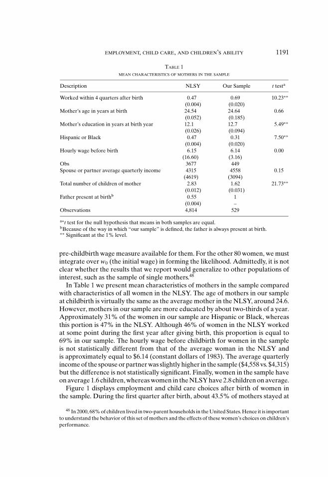
TABLE 1MEAN CHARACTERISTICS OF MOTHERS IN THE SAMPLE
Description NLSY Our Sample t testa
Worked within 4 quarters after birth 0.47 0.69 10.23∗∗(0.004) (0.020)
Mother’s age in years at birth 24.54 24.64 0.66(0.052) (0.185)
Mother’s education in years at birth year 12.1 12.7 5.49∗∗(0.026) (0.094)
Hispanic or Black 0.47 0.31 7.50∗∗(0.004) (0.020)
Hourly wage before birth 6.15 6.14 0.00(16.60) (3.16)
Obs 3677 449Spouse or partner average quarterly income 4315 4558 0.15
(4619) (3094)Total number of children of mother 2.83 1.62 21.73∗∗
(0.012) (0.031)Father present at birthb 0.55 1
(0.004) –Observations 4,814 529
a∗t test for the null hypothesis that means in both samples are equal.bBecause of the way in which “our sample” is defined, the father is always present at birth.∗∗ Significant at the 1% level.
pre-childbirth wage measure available for them. For the other 80 women, we mustintegrate over w0 (the initial wage) in forming the likelihood. Admittedly, it is notclear whether the results that we report would generalize to other populations ofinterest, such as the sample of single mothers.48
In Table 1 we present mean characteristics of mothers in the sample comparedwith characteristics of all women in the NLSY. The age of mothers in our sampleat childbirth is virtually the same as the average mother in the NLSY, around 24.6.However, mothers in our sample are more educated by about two-thirds of a year.Approximately 31% of the women in our sample are Hispanic or Black, whereasthis portion is 47% in the NLSY. Although 46% of women in the NLSY workedat some point during the first year after giving birth, this proportion is equal to69% in our sample. The hourly wage before childbirth for women in the sampleis not statistically different from that of the average woman in the NLSY andis approximately equal to $6.14 (constant dollars of 1983). The average quarterlyincome of the spouse or partner was slightly higher in the sample ($4,558 vs. $4,315)but the difference is not statistically significant. Finally, women in the sample haveon average 1.6 children, whereas women in the NLSY have 2.8 children on average.
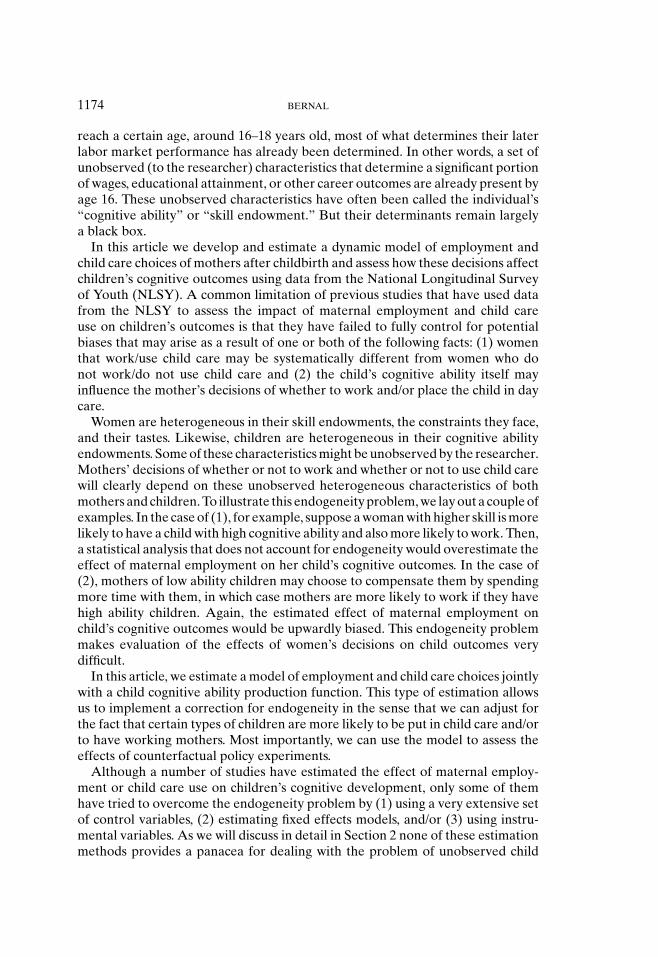
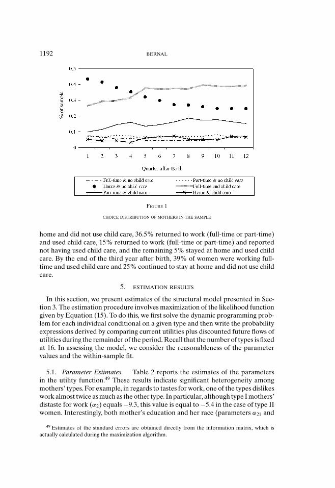
Figure 1 displays employment and child care choices after birth of women inthe sample. During the first quarter after birth, about 43.5% of mothers stayed at
48 In 2000, 68% of children lived in two-parent households in the United States. Hence it is importantto understand the behavior of this set of mothers and the effects of these women’s choices on children’sperformance.
1192 BERNAL
FIGURE 1
CHOICE DISTRIBUTION OF MOTHERS IN THE SAMPLE
home and did not use child care, 36.5% returned to work (full-time or part-time)and used child care, 15% returned to work (full-time or part-time) and reportednot having used child care, and the remaining 5% stayed at home and used childcare. By the end of the third year after birth, 39% of women were working full-time and used child care and 25% continued to stay at home and did not use childcare.
5. ESTIMATION RESULTS
In this section, we present estimates of the structural model presented in Sec-tion 3. The estimation procedure involves maximization of the likelihood functiongiven by Equation (15). To do this, we first solve the dynamic programming prob-lem for each individual conditional on a given type and then write the probabilityexpressions derived by comparing current utilities plus discounted future flows ofutilities during the remainder of the period. Recall that the number of types is fixedat 16. In assessing the model, we consider the reasonableness of the parametervalues and the within-sample fit.
5.1. Parameter Estimates. Table 2 reports the estimates of the parametersin the utility function.49 These results indicate significant heterogeneity amongmothers’ types. For example, in regards to tastes for work, one of the types dislikeswork almost twice as much as the other type. In particular, although type I mothers’distaste for work (α2) equals −9.3, this value is equal to −5.4 in the case of type IIwomen. Interestingly, both mother’s education and her race (parameters α21 and
49 Estimates of the standard errors are obtained directly from the information matrix, which isactually calculated during the maximization algorithm.
EMPLOYMENT, CHILD CARE, AND CHILDREN’S ABILITY 1193
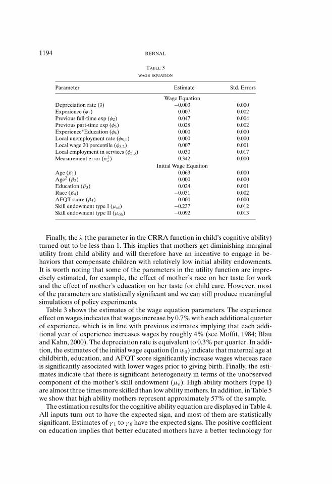
TABLE 2UTILITY FUNCTION
Parameter Estimate Std. Errors
Consumption (α1) 0.36 0.01Mother’s education on taste for work (α21) −0.27 0.04Mother’s race on taste for work (α22) −0.37 0.28Disutility from work (α2) Type I −9.30 0.53Disutility from work (α2) Type II −5.41 0.58Utility from child’s ability (α3) 0.00 0.02Ability function (λ) 0.46 0.20Mother’s education in taste for child care (α41) −0.02 0.02Mother’s race in taste for child care (α42) 0.39 0.12Utility from child care (α4) Type I −0.27 0.24Utility from child care (α4) Type II 7.92 1.15Cost of no child care if working (α5) −4.67 0.08Cost of initiating child care (α6) −5.08 0.03Extra cost of using child care in qtr 1 (α7) −0.26 0.16Extra cost of using child care during 1st year (α8) −1.20 0.06Child care cost (cc) 156.8 70.8
α22) decrease the disutility from work. To have a clearer interpretation of someof these parameters, we express them in terms of consumption units. Averageconsumption per quarter is $6,350. For example, working full time during a givenperiod reduces consumption by $919 for women type I (high disutility from work)and $535 for type II women (low disutility from work). In addition, in Table 5 weshow that approximately 43% of the mothers in the sample correspond to type II(low disutility from work).
Women are quite different in their tastes for child care. Although one of thetypes derives disutility from child care (α4 = −.271), the other type derives a highutility from using child care in any given period (α4 = 7.92).50 Race significantlyincreases the utility derived from using child care51 whereas education is not signif-icantly associated with tastes for child care (parameters α41 and α42, respectively).The disutility from using child care for women type I is equivalent to −$27 whereasthe utility of using child care in the case of women type II is approximately $783.
The cost to a parent of working without using child care is $462 (−4.66 inutility units). The cost of initiating child care (if never used before) is about $502.The extra cost associated with using child care during the first quarter after birthis $26 and the extra cost of using child care before the child is one year old isapproximately $119. Finally, the cost of child care per quarter is estimated to be$156 (dollars of 1983), which corresponds approximately to $324 in 2007. Althoughthis amount may seem small, it is important to remember that this estimationaverages over various types of child care, which can have very different qualitiesand prices, including child care provided by relatives (which is in most cases free).
50 According to the results presented in Table 5 only 23% of women in the sample correspond totype II (high utility from using child care).
51 Race is a dummy variable that equals 1 for nonwhites.
1194 BERNAL
TABLE 3WAGE EQUATION
Parameter Estimate Std. Errors
Wage EquationDepreciation rate (δ) −0.003 0.000Experience (φ1) 0.007 0.002Previous full-time exp (φ2) 0.047 0.004Previous part-time exp (φ3) 0.028 0.002Experience∗Education (φ4) 0.000 0.000Local unemployment rate (φ5,1) 0.000 0.000Local wage 20 percentile (φ5,2) 0.007 0.001Local employment in services (φ5,3) 0.030 0.017Measurement error (σ 2
ε) 0.342 0.000Initial Wage Equation
Age (β1) 0.063 0.000Age2 (β2) 0.000 0.000Education (β3) 0.024 0.001Race (β4) −0.031 0.002AFQT score (β5) 0.000 0.000Skill endowment type I (µol) −0.237 0.012Skill endowment type II (µoh) −0.092 0.013
Finally, the λ (the parameter in the CRRA function in child’s cognitive ability)turned out to be less than 1. This implies that mothers get diminishing marginalutility from child ability and will therefore have an incentive to engage in be-haviors that compensate children with relatively low initial ability endowments.It is worth noting that some of the parameters in the utility function are impre-cisely estimated, for example, the effect of mother’s race on her taste for workand the effect of mother’s education on her taste for child care. However, mostof the parameters are statistically significant and we can still produce meaningfulsimulations of policy experiments.
Table 3 shows the estimates of the wage equation parameters. The experienceeffect on wages indicates that wages increase by 0.7% with each additional quarterof experience, which is in line with previous estimates implying that each addi-tional year of experience increases wages by roughly 4% (see Moffit, 1984; Blauand Kahn, 2000). The depreciation rate is equivalent to 0.3% per quarter. In addi-tion, the estimates of the initial wage equation (ln w0) indicate that maternal age atchildbirth, education, and AFQT score significantly increase wages whereas raceis significantly associated with lower wages prior to giving birth. Finally, the esti-mates indicate that there is significant heterogeneity in terms of the unobservedcomponent of the mother’s skill endowment (µo). High ability mothers (type I)are almost three times more skilled than low ability mothers. In addition, in Table 5we show that high ability mothers represent approximately 57% of the sample.
The estimation results for the cognitive ability equation are displayed in Table 4.All inputs turn out to have the expected sign, and most of them are statisticallysignificant. Estimates of γ 1 to γ 6 have the expected signs. The positive coefficienton education implies that better educated mothers have a better technology for
EMPLOYMENT, CHILD CARE, AND CHILDREN’S ABILITY 1195
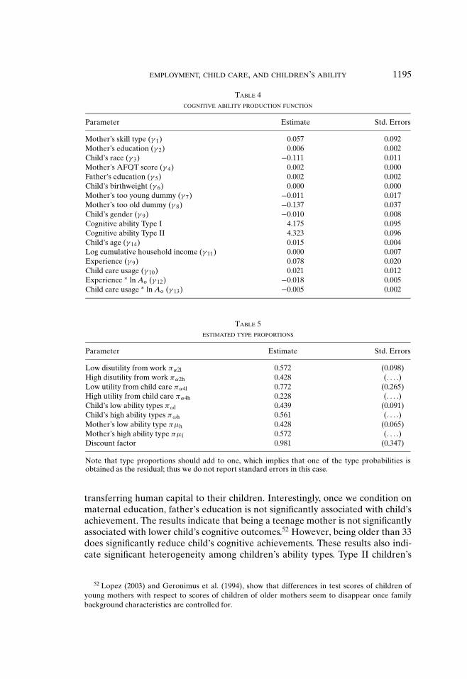
TABLE 4COGNITIVE ABILITY PRODUCTION FUNCTION
Parameter Estimate Std. Errors
Mother’s skill type (γ 1) 0.057 0.092Mother’s education (γ 2) 0.006 0.002Child’s race (γ 3) −0.111 0.011Mother’s AFQT score (γ 4) 0.002 0.000Father’s education (γ 5) 0.002 0.002Child’s birthweight (γ 6) 0.000 0.000Mother’s too young dummy (γ 7) −0.011 0.017Mother’s too old dummy (γ 8) −0.137 0.037Child’s gender (γ 9) −0.010 0.008Cognitive ability Type I 4.175 0.095Cognitive ability Type II 4.323 0.096Child’s age (γ 14) 0.015 0.004Log cumulative household income (γ 11) 0.000 0.007Experience (γ 9) 0.078 0.020Child care usage (γ 10) 0.021 0.012Experience ∗ ln Ao (γ 12) −0.018 0.005Child care usage ∗ ln Ao (γ 13) −0.005 0.002
TABLE 5ESTIMATED TYPE PROPORTIONS
Parameter Estimate Std. Errors
Low disutility from work πα2l 0.572 (0.098)High disutility from work πα2h 0.428 (. . . .)Low utility from child care πα4l 0.772 (0.265)High utility from child care πα4h 0.228 (. . . .)Child’s low ability types πωl 0.439 (0.091)Child’s high ability types πωh 0.561 (. . . .)Mother’s low ability type πµh 0.428 (0.065)Mother’s high ability type πµl 0.572 (. . . .)Discount factor 0.981 (0.347)
Note that type proportions should add to one, which implies that one of the type probabilities isobtained as the residual; thus we do not report standard errors in this case.
transferring human capital to their children. Interestingly, once we condition onmaternal education, father’s education is not significantly associated with child’sachievement. The results indicate that being a teenage mother is not significantlyassociated with lower child’s cognitive outcomes.52 However, being older than 33does significantly reduce child’s cognitive achievements. These results also indi-cate significant heterogeneity among children’s ability types. Type II children’s
52 Lopez (2003) and Geronimus et al. (1994), show that differences in test scores of children ofyoung mothers with respect to scores of children of older mothers seem to disappear once familybackground characteristics are controlled for.
1196 BERNAL
FIGURE 2
EFFECT OF MATERNAL EMPLOYMENT ON COGNITIVE ABILITY: d ln St/dEt = 0.078 − 0.018 ln Ao
unobserved ability endowment is 15% higher than type II children’s (4.32 vs.4.17).53
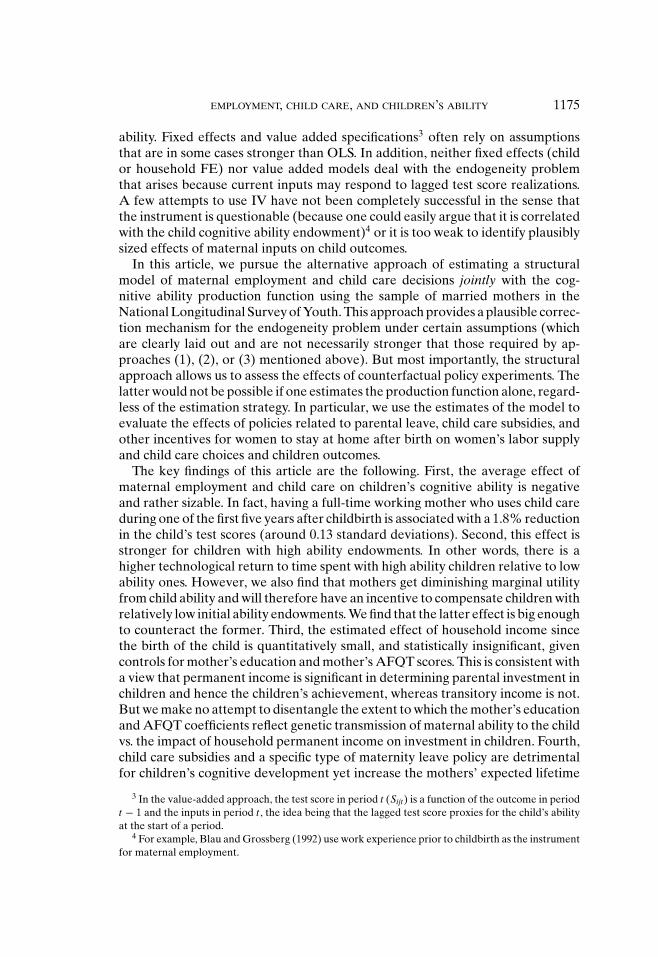
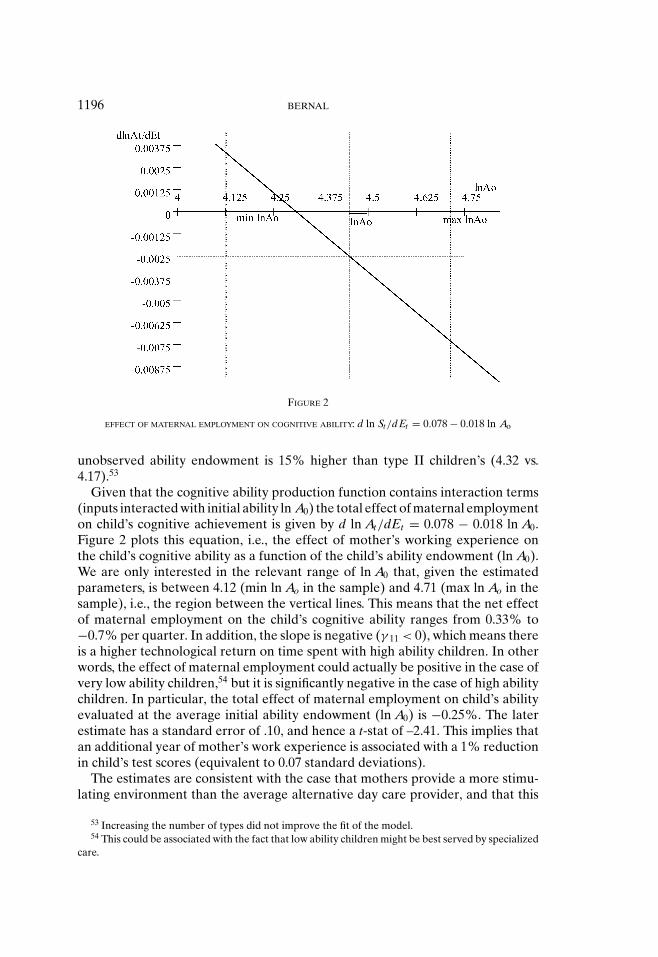
Given that the cognitive ability production function contains interaction terms(inputs interacted with initial ability ln A0) the total effect of maternal employmenton child’s cognitive achievement is given by d ln At/dEt = 0.078 − 0.018 ln A0.Figure 2 plots this equation, i.e., the effect of mother’s working experience onthe child’s cognitive ability as a function of the child’s ability endowment (ln A0).We are only interested in the relevant range of ln A0 that, given the estimatedparameters, is between 4.12 (min ln Ao in the sample) and 4.71 (max ln Ao in thesample), i.e., the region between the vertical lines. This means that the net effectof maternal employment on the child’s cognitive ability ranges from 0.33% to−0.7% per quarter. In addition, the slope is negative (γ 11 < 0), which means thereis a higher technological return on time spent with high ability children. In otherwords, the effect of maternal employment could actually be positive in the case ofvery low ability children,54 but it is significantly negative in the case of high abilitychildren. In particular, the total effect of maternal employment on child’s abilityevaluated at the average initial ability endowment (ln A0) is −0.25%. The laterestimate has a standard error of .10, and hence a t-stat of –2.41. This implies thatan additional year of mother’s work experience is associated with a 1% reductionin child’s test scores (equivalent to 0.07 standard deviations).
The estimates are consistent with the case that mothers provide a more stimu-lating environment than the average alternative day care provider, and that this
53 Increasing the number of types did not improve the fit of the model.54 This could be associated with the fact that low ability children might be best served by specialized
care.

EMPLOYMENT, CHILD CARE, AND CHILDREN’S ABILITY 1197
FIGURE 3
EFFECT OF CHILD CARE USE ON COGNITIVE ABILITY: d ln St/dCt = 0.021 − 0.005 lnAo
effect is stronger for higher ability children.55 However, given the specification ofthe utility function, i.e., the CRRA functional form for child’s cognitive ability, weare allowing for a compensation effect in the sense that parents may compensatelow ability type children by devoting more time to them, depending on the curva-ture parameter λ. The net effect can only become clear by studying individuals’choices, which we do in the next section.
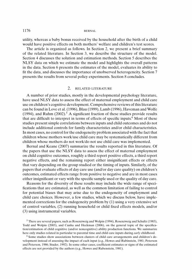
Similarly, the total effect of child care use on the child’s cognitive ability is givenby d ln At/dCt = 0.021 − 0.005 ln A0. This expression is plotted in Figure 3. Ascan be observed, the net effect of child care use on a child’s cognitive ability inthe relevant range of ln A0 ranges from −0.02% to −0.32% per quarter. The neteffect evaluated at the average of ln A0 is −0.19%. This estimate has a standarderror of .11, and hence a t-stat of –1.67. This means that an additional year ofchild care use is associated with a reduction of approximately 0.8% in child’s testscores (equivalent to 0.05 standard deviations). Again, given that γ 12 < 0, thereis a higher technological return to having high ability children spend less time atchild care than in the case of low ability children.
In sum, the total effect of an additional quarter of maternal working experi-ence and child care use on children’s test scores is −0.44%.56 This estimate has astandard error of .13, and hence a t-stat of –3.32. This means that having a motherthat works full-time and uses child care during one whole year (within the first
55 We also find that high ability children are in fact associated with high ability mothers. In thiscase, this result could also be interpreted as highly skilled mothers time inputs having stronger positiveeffect on children.
56 The first column in Table 7 shows the results from running the cognitive ability Equation (1) byOLS using the same sample of women. The total effect of maternal employment and child care use onchilds’ outcomes is around −0.12% per quarter.
1198 BERNAL
five years after the birth of the child) is associated with a reduction in test scoresof approximately 1.8% (which is equivalent to 0.13 standard deviations).
Finally, the estimated effect of household income since the birth of the childis quantitatively small and statistically insignificant (see Table 4), given controlsfor mother’s education and mother’s AFQT scores. This is consistent with a viewthat permanent income is significant in determining parental investment in chil-dren and hence the children’s achievement, whereas transitory income is not.57
However, we do not attempt to disentangle the role of (i) genetic transmission ofparental ability from (ii) the impact of household permanent income on invest-ment in children.
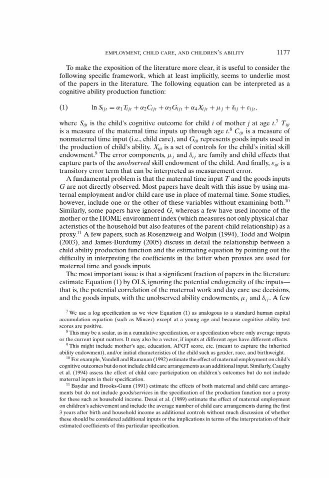
5.2. Model Fit. Figure 4 depicts the fit of the model to the choice distribu-tions in Figure 1, based on a simulation of 8,000 individuals. As can be observed,the model matches the data quite well, in particular, in the case of the most chosenalternatives, i.e., working full-time or part-time and using child care and stayingat home without child care.58 Finally, predicted period-by-period transitions, pre-dicted wages by mother’s education and age, as well as predicted log averagescores by age and by characteristics of the mother (figures not shown) fit the dataquite closely.
5.3. Understanding Unobserved Heterogeneity. As has been emphasized,there is significant heterogeneity among individuals by unobserved characteristics.It would be interesting to try to describe these types even if the model is silent onhow types are determined. As was mentioned in an earlier section, according tothe parameter estimates, there is a higher technological return of spending timewith higher ability children (since the parameter γ 11 turned out to be negative)but women derive higher marginal utility from spending time with lower abilitychildren (given that λ < 1). Because these two effects go in opposite directions,whether mothers engage in compensating behaviors such that they spend moretime (or use less child care) with low ability children is an empirical issue that wenow turn to discuss.
Table 6 shows the proportion of mothers of low ability endowment childrenwho work (per period) compared to the proportion of mothers of high abilityendowment children who do. The right panel shows the same comparison in thecase of child care use. One can observe that, on average, mothers of low abilitychildren tend to work less and use less child care. For instance, during the firstquarter after birth, 2.7 percentage points (5% ) less women work and 1 percentagepoints less women use child care. The same is true for every period after birth. Thispattern implies that mothers of low ability children compensate them by spending
57 This finding is reminiscent of the findings by Keane and Wolpin (2001) and Cameron and Heck-man (1998) to the effect that transitory fluctuations in parental income have little effect on collegeattendance decisions by youth. In addition, it is consistent with findings by Blau (1999) and Carneiroand Heckman (2002) according to which permanent household income is significant in determininginvestments in children whereas transitory income is not.
58 χ2 goodness-of-fit test statistics (not reported) confirm the graphical results, with the fit beingrejected in very few periods.
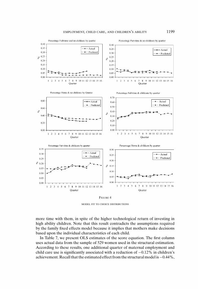
EMPLOYMENT, CHILD CARE, AND CHILDREN’S ABILITY 1199
FIGURE 4
MODEL FIT TO CHOICE DISTRIBUTIONS
more time with them, in spite of the higher technological return of investing inhigh ability children. Note that this result contradicts the assumptions requiredby the family fixed effects model because it implies that mothers make decisionsbased upon the individual characteristics of each child.
In Table 7, we present OLS estimates of the score equation. The first columnuses actual data from the sample of 529 women used in the structural estimation.According to these results, one additional quarter of maternal employment andchild care use is significantly associated with a reduction of −0.12% in children’sachievement. Recall that the estimated effect from the structural model is −0.44%,
1200 BERNAL
TABLE 6MOTHER’S CHOICES BY CHILD’S ABILITY ENDOWMENT
(% OF WOMEN CHOOSING EACH ALTERNATIVE)
Work Child Care
Mothers of Mothers of
Quarter Low High Low Highafter Ability Ability Ability Abilitybirth Child Child Difference Child Child Difference
1 54.40 57.16 2.76 45.13 45.99 0.862 56.74 60.97 4.23 49.16 49.90 0.753 57.58 62.60 5.01 49.91 50.67 0.764 57.58 60.88 3.29 49.63 50.86 1.235 60.11 64.22 4.11 57.02 60.50 3.476 61.05 66.41 5.36 59.27 61.64 2.377 62.08 65.36 3.28 58.80 62.79 3.988 62.17 64.60 2.43 60.11 62.21 2.1016 61.52 66.41 4.90 61.61 63.84 2.23
Based on a simulation of 8.000 individuals.
which means that OLS estimates of the maternal employment and child care useon children’s achievement are indeed upwardly biased as expected. That is, oncewe correct for the endogeneity problem, the effect significantly declines relativeto the OLS estimates. In addition, household cumulative income turns out tobe positive and significant. However, the effect is quantitatively very small. Inparticular, a 1% increase in household income is associated with an increase of0.009% in children’s test scores.
Column (2) shows the same OLS estimation using simulated data generatedby the model and the estimated parameter vector. Interestingly, results from theestimation on simulated data turn out to be very close to the OLS estimation onactual data.59 These results indicate that the effect of an additional quarter ofmaternal employment and child care use is around −0.18%. This means that themodel is in fact generating the same endogeneity bias present in the data and itgoes in the expected direction.
Finally, column (3) shows OLS estimates using simulated data again but wecondition on both mother’s types and children’s types (which are known in thesimulation). In other words, we can assign ω-types and µ0-types and include theseas additional controls in the regression. We observe that once we control for unob-served types, the effect of maternal employment and child care use is significantlylarger. In particular, an additional quarter of maternal work experience and childcare use is associated with a 0.24% reduction in children’s achievements. Thatmeans that once we partially control for the sources of endogeneity we signifi-cantly reduce the bias.
59 These regressions are based on a simulation of 8,000 individuals whereas the actual data contains529 observations. The fact that the size of the simulated data is bigger can be the reason that somecoefficients turn out to be significant whereas they were insignificant when estimated on actual data.
EMPLOYMENT, CHILD CARE, AND CHILDREN’S ABILITY 1201
TABLE 7OLS ESTIMATION OF THE TEST SCORE EQUATION
Simulated DataActual data
(1) (2) (3)
Work experience + child care use −0.0012 −0.0018 −0.0024(0.0006)∗ (0.0001)∗∗ (0.0008)∗∗
Log(Cumulative Income) 0.0096 0.0090 0.0006(0.0053)∗ (0.0029)∗∗ (0.0022)
Gender 0.0108 −0.0027 −0.0044(0.0078) (0.0022) (0.0016)
Birthweight 0.0001 0.0002 0.0003(0.0002) (0.0001)∗∗ (0.0001)∗∗
Mother’s education −0.0014 0.0101 0.0054(0.0027) (0.0007)∗∗ (0.0005)∗∗
Mother’s AFQT 0.0014 0.0012 0.0019(0.0002)∗∗ (0.0001)∗∗ (0.0004)∗∗
I[age<18] −0.0187 −0.0003 −0.0262(0.0189) (0.0069)∗∗ (0.0052)∗∗
I[age>=33] −0.0696 −0.1021 −0.1077(0.0302)∗∗ (0.0087)∗∗ (0.0065)∗∗
Race −0.0663 −0.0877 −0.0935(0.0093)∗∗ (0.0025)∗∗ (0.0019)∗∗
Father’s education 0.0098 0.0016 0.0011(0.0020)∗∗ (0.0005)∗∗ (0.0004)∗∗
Child’s age 0.0164 0.0182 0.0210(0.0066)∗∗ (0.0026)∗∗ (0.0015)∗∗
PPVT dummy −0.0943 −0.0921 −0.0741(0.0134)∗∗ (0.0047)∗∗ (0.0035)∗∗
MATH dummy −0.0602 −0.0508 −0.0344(0.0097)∗∗ (0.0030)∗∗ (0.0022)∗∗
Constant 4.4605 4.3478(0.0413)∗∗ (0.0306)∗∗
Mother type 1 + Child type 1 4.3853(0.0233)∗∗
Mother type 1 + Child type 2 4.3769(0.0230)∗∗
Mother type 2 + Child type 1 4.5065(0.0232)∗∗
Mother type 2 + Child type 2 4.5017(0.0230)∗∗
R2 0.241 0.253 0.414
(1) OLS estimated with actual data.(2) OLS estimated with simulated data.(3) OLS estimated with simulated data but assigning mother–child types.Standard errors reported do not take into account the estimation error on the model parameters.
6. POLICY EXPERIMENTS
In this section, we evaluate the effect of various policies on women’s choicedistributions and children’s average test scores.
1202 BERNAL
TABLE 8THE EFFECT OF A 35% CHILD CARE SUBSIDY ON AVERAGE TEST
SCORES (PERCENTAGE DIFFERENCE IN TEST SCORES WITH RESPECT
TO THE BASELINE)
Test and child’s age % change in avg. test scores
PPVT age 3 −1.07PPVT age 4 −1.87PPVT age 5 −0.24MATH age 5 −1.19MATH age 6 −0.94READ age 5 −0.82READ age 6 −0.23
Based on a simulation of 8000 individuals.
6.1. Child Care Subsidy. The first experiment involves a 35% child caresubsidy. In particular, the parameter cc is reduced from its estimated value of$156.8 to $102. As expected, the percentage of women choosing alternatives thatinclude child care increases with respect to the baseline case. On average, there isan increase of 4 percentage points per period in the number of women that nowchoose to use child care (choice distribution not shown).
However, a priori it is not obvious what will happen with employment choicesonce the subsidy is introduced. On the one hand, there is a substitution effect inthe sense that the availability of cheaper child care might allow women to workmore. On the other hand, there is an income effect given that the subsidy increaseshousehold income, and hence might induce a reduction in the hours of work. Theoverall effect of the subsidy is to increase the percentage of women working inalmost every period after childbirth by approximately 1 percentage point, whichimplies that the substitution effect dominates.
Table 8 displays the percentage difference in average log scores by ability type inthe 35% child care subsidy case with respect to the baseline. The results indicatethat the introduction of a subsidy is associated with a reduction in test scoresat all ages. This reduction ranges from 0.23% to 1.8% depending on the testand the age of the child. Given the fact that child care has a negative effect onthe child’s cognitive ability, the incentive for mothers to move into child carealternatives is detrimental to children’s scores even if it seems to increase parents’utility.60
6.2. Maternity Leave Policy. In this section, we analyze a maternity leavepolicy according to which there is no wage penalty for time out of the labor marketafter giving birth. In particular, we do this by setting the wage depreciation rateδ at 0. This means that if a woman did not work for a few periods after giving
60 One can calculate the mother’s mean expected present value of lifetime utility at t = 1 and observethat it increases on average 0.3% once the child care subsidy is introduced.
EMPLOYMENT, CHILD CARE, AND CHILDREN’S ABILITY 1203
birth, her re-employment wage is drawn from the same wage distribution she hadbefore giving birth.61
Once the wage depreciation rate is set at 0 a higher percentage of women chooseto work full-time relative to the baseline case, whereas less choose to either stay athome or work part-time (choice distribution not shown). For example, in period 4the total percentage of women choosing to work increases by 6 percentage points,and the proportion of mothers choosing to use child care raises by 5 percentagepoints.
Intuitively, women are still getting zero wages during the time they are awayfrom the labor market after childbirth but the opportunity cost of staying at homehas now increased relative to the baseline scenario. Forgone wages are higherduring the current period, and the discounted stream of future wages has increasedas well. The expected gain derived from staying home with their children throughtheir increased cognitive ability is not enough to compensate for the loss in termsof forgone wages and, hence, women choose to work more.
As expected this has the effect of reducing average scores given that mothers arenot only working more but also using more child care. The reduction in averagetest scores with respect to the baseline case ranges from 0.1% to 1% dependingon the test and the age of the child. Mothers’ mean expected present value oflifetime utility at time t = 1 is increased by 0.6% with respect to the benchmarkcase. It is difficult to assess whether this type of policy is effective or not given thefact that although it increases women’s lifetime utility, it decreases children’s testscores.
6.3. Baby Bonus. Finally, we assess the impact on women’s decisions andchildren’s average test scores of a $250 quarterly baby bonus after the birth ofa child and until he or she is 5 years old.62 In this case, fewer women choosealternatives that include work and more women decide to stay at home with theirchildren (choice distributions are not shown).
Table 9 reports the proportion of women who choose each alternative in thebaseline case as well as in the $250 baby bonus scenario in period 4. The last columnshows the difference (in percentage points) between these. As can be observed,there is a reduction in the proportion of women working (full-time and part-time)of 3.8 percentage points and a reduction in the proportion of women using child
61 An alternative way to model the maternity leave policy would be to allow for the possibilityof paid benefits during a given leave period. However, in this case the state space would have to bealtered to account for the new state variable. In the United States the law requires only that employershold the mother’s job for 12 weeks after giving birth but does not mandate paid benefits during thistime. Hence it seems reasonable to model this policy as one in which women are not penalized in thesense that their wage after childbirth is not reduced depending on the time they spent out of the labormarket after giving birth.
62 To give a few examples, Australia just very recently implemented a baby bonus for a maximumof up to $2,500 per annum over five years. The minimum entitlement is $500 per year. In Singapore,the baby bonus amounts to $3,000 for the second child and $6000 for the third child. Parents in Japanget a $70 allowance a month for the first two children until they enter pre-school. Also, a per-child taxdeduction as those that have been implemented in the United States would be analogous to this typeof bonus.
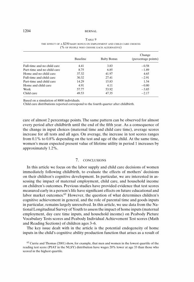
1204 BERNAL
TABLE 9THE EFFECT OF A $250 BABY BONUS ON EMPLOYMENT AND CHILD CARE CHOICES
(% OF PEOPLE WHO CHOOSE EACH ALTERNATIVE)
ChangeBaseline Baby Bonus (percentage points)
Full-time and no child care 4.41 3.83 −0.58Part-time and no child care 8.75 6.85 −1.89Home and no child care 37.32 41.97 4.65Full-time and child care 30.32 27.41 −2.91Part-time and child care 14.29 15.83 1.54Home and child care 4.91 4.11 −0.80Work 57.77 53.92 −3.85Child care 49.53 47.35 −2.17
Based on a simulation of 8000 individuals.Child care distributions reported correspond to the fourth quarter after childbirth.
care of almost 2 percentage points. The same pattern can be observed for almostevery period after childbirth until the end of the fifth year. As a consequence ofthe change in input choices (maternal time and child care time), average scoresincrease for all tests and all ages. On average, the increase in test scores rangesfrom 0.1% to 0.8% depending on the test and age of the child. At the same time,women’s mean expected present value of lifetime utility in period 1 increases byapproximately 1.2%.
7. CONCLUSIONS
In this article we focus on the labor supply and child care decisions of womenimmediately following childbirth, to evaluate the effects of mothers’ decisionson their children’s cognitive development. In particular, we are interested in as-sessing the impact of maternal employment, child care, and household incomeon children’s outcomes. Previous studies have provided evidence that test scoresmeasured early in a person’s life have significant effects on future educational andlabor market outcomes.63 However, the question of what determines children’scognitive achievement in general, and the role of parental time and goods inputsin particular, remains largely unresolved. In this article, we use data from the Na-tional Longitudinal Survey of Youth to assess the impact of home inputs (maternalemployment, day care time inputs, and household income) on Peabody PictureVocabulary Tests scores and Peabody Individual Achievement Test scores (Mathand Reading Sections) of children ages 3–6.
The key issue dealt with in the article is the potential endogeneity of homeinputs in the child’s cognitive ability production function that arises as a result of
63 Currie and Thomas (2001) show, for example, that men and women in the lowest quartile of thereading test score (PIAT in the NLSY) distribution have wages 20% lower at age 33 than those whoscored in the highest quartile.
EMPLOYMENT, CHILD CARE, AND CHILDREN’S ABILITY 1205
the existence of unobserved characteristics of both mothers and children. Womenare heterogeneous in both the constraints they face and their tastes. At the sametime, children are heterogeneous in their cognitive endowments. As we would ex-pect, mothers’ decisions with respect to working when children are young and/orplacing children in child care are influenced by these heterogeneous characteris-tics. Hence, children of working women or children of women who use child carewill differ systematically from those whose mothers stay at home or do not usechild care. Estimation of a structural model of women’s employment and childcare choices jointly with a cognitive ability production function is suggested asan alternative way of implementing a correction mechanism for this endogeneityproblem. Most importantly, estimation of the structural model allows us to explorethe effects of counterfactual policy experiments on women’s choices and children’soutcomes that we would not be able to do with the ability production functionalone.
Results suggest that the effects of maternal employment and child care duringthe first five years of life of the child are rather sizable. In fact, an additional yearof full-time work is associated with a reduction of about 1% in test scores, and anadditional year of child care use is associated with a reduction of approximately0.8% in children’s achievement. This means that having a full-time working motherthat uses child care during an entire year (within the first five years after the birthof the child) is associated with a 1.8% (0.13 standard deviations) reduction inability test scores. Furthermore, we find that this effect is stronger for high abilitychildren. In other words, there is a higher technological return to spending timewith high ability children relative to time spent with low ability children. However,we also find that mothers get diminishing marginal utility from child ability, andwill therefore have an incentive to compensate children with relatively low initialability endowments. We find that the latter effect is big enough to counteract theformer.
In addition, the estimated effect of household income since the birth of thechild is quantitatively small and statistically insignificant, given controls formother’s education and mother’s AFQT scores. This is consistent with a viewthat permanent income is significant in determining parental investment in chil-dren, and hence the children’s achievement, whereas transitory income is not.But we make no attempt to disentangle the extent to which the mother’s ed-ucation and AFQT coefficients reflect genetic transmission of maternal abilityto the child vs. the impact of household permanent income on investment inchildren.
The results of the policy experiments suggest that both child care subsi-dies and maternity leave entitlements can be detrimental for pre-school agedchildren’s cognitive outcomes, while increasing mothers’ expected lifetime util-ity. On the one hand, child care subsidies provide incentives for women whoderive high disutility from work and/or high utility from child care to choose al-ternatives that include child care. This has a negative effect on children’s averagescores.
On the other hand, by setting the wage depreciation at zero, in other words,eliminating the wage penalty that a woman would incur depending on the number
1206 BERNAL
of periods she was away from the labor market after giving birth, children aremade worse off. Intuitively, given the fact that women do not receive a wage (ora portion of it) while away from the labor market and forgone wages are higherrelative to the case in which the depreciation rate is nonzero, women decide towork more under the new scenario. Not only is the current forgone wage higherbut so is the expected stream of future wages. Hence, if the gain derived fromincreased child’s cognitive ability is smaller than the opportunity cost of stayingat home, women choose to work more with the expected detrimental effect thatthis has on children’s average scores.
Finally, the effect of a $250 quarterly baby bonus after the birth of a child anduntil he/she goes to primary school at age 5 has a positive impact on both mothersand children. On the one hand, mean expected present value of lifetime utility ofmothers is increased by 1.2% and on the other hand average scores of childrenincrease by about 0.5%. The increase in household’s income provides an incentivefor women to work less and stay at home with their children at the same time thatit acts as a disincentive for child care use. Therefore, the net effect is to increasechildren’s cognitive ability as well as mothers’ utility.
We do not claim that the estimated effects and the results of the policy exper-iments reported here can be generalizable. As a matter of fact, we have used arestricted sample of women in the NLSY to estimate the model. In particular, wehave used mothers that are married and women that do not have an additionalchild during the five year period following childbirth. Hence, the results shouldonly be thought as applicable to this specific subset of women.64
In this article, we have assumed that there is a homogeneous type of child care.An interesting extension of the model would be to include quality of child care as achoice variable of the mother. One might argue that the result according to whichmaternal employment has a significant and sizable negative effect on children’scognitive ability is driven by the fact that most of the child care provided is of lowquality. Clearly, introducing the quality of child care in the model might changethe results in very interesting ways. A woman with higher wage might be able topurchase child care services of very high quality in which case it will not be soclear that her time investments will be as valuable.
Finally, the results could be sensitive to changes in the assumptions about whatthe mother knows about her child. One could allow, for example, the child’s un-observed ability endowment (ωκ) to be a composite of two components, one ofwhich is observed by the mother. It is difficult to predict in which direction theresults would change but it is plausible to think that this could describe parents’behavior better.
64 Bernal and Keane (2008) estimate a quasi-structural version of a model very similar to the onepresented in this article using the sample of single mothers in the NLSY. In addition, Bernal and Keane(2007) use a set of welfare rules and local demand conditions as instrumental variables to estimate acognitive ability production function using the same sample of single mothers (NLSY). The estimatedeffects of child care use on children’s cognitive outcomes in both papers are strikingly similar to theones reported here for the sample of married women.
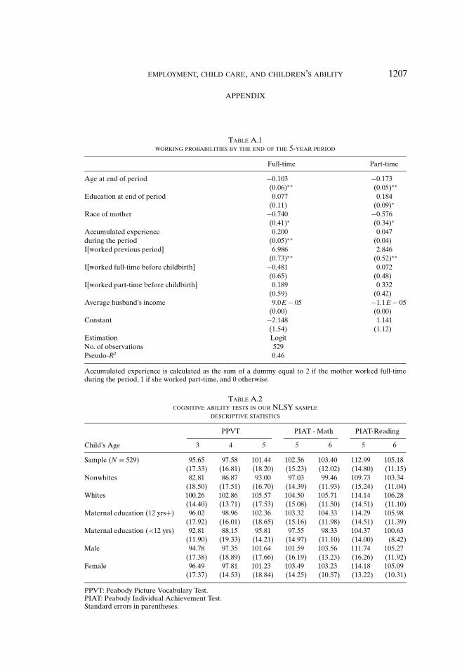
EMPLOYMENT, CHILD CARE, AND CHILDREN’S ABILITY 1207
APPENDIX
TABLE A.1WORKING PROBABILITIES BY THE END OF THE 5-YEAR PERIOD
Full-time Part-time
Age at end of period −0.103 −0.173(0.06)∗∗ (0.05)∗∗
Education at end of period 0.077 0.184(0.11) (0.09)∗
Race of mother −0.740 −0.576(0.41)∗ (0.34)∗
Accumulated experience 0.200 0.047during the period (0.05)∗∗ (0.04)I[worked previous period] 6.986 2.846
(0.73)∗∗ (0.52)∗∗
I[worked full-time before childbirth] −0.481 0.072(0.65) (0.48)
I[worked part-time before childbirth] 0.189 0.332(0.59) (0.42)
Average husband’s income 9.0E − 05 −1.1E − 05(0.00) (0.00)
Constant −2.148 1.141(1.54) (1.12)
Estimation LogitNo. of observations 529Pseudo-R2 0.46
Accumulated experience is calculated as the sum of a dummy equal to 2 if the mother worked full-timeduring the period, 1 if she worked part-time, and 0 otherwise.
TABLE A.2COGNITIVE ABILITY TESTS IN OUR NLSY SAMPLE
DESCRIPTIVE STATISTICS
PPVT PIAT - Math PIAT-Reading
Child’s Age 3 4 5 5 6 5 6
Sample (N = 529) 95.65 97.58 101.44 102.56 103.40 112.99 105.18(17.33) (16.81) (18.20) (15.23) (12.02) (14.80) (11.15)
Nonwhites 82.81 86.87 93.00 97.03 99.46 109.73 103.34(18.50) (17.51) (16.70) (14.39) (11.93) (15.24) (11.04)
Whites 100.26 102.86 105.57 104.50 105.71 114.14 106.28(14.40) (13.71) (17.53) (15.08) (11.50) (14.51) (11.10)
Maternal education (12 yrs+) 96.02 98.96 102.36 103.32 104.33 114.29 105.98(17.92) (16.01) (18.65) (15.16) (11.98) (14.51) (11.39)
Maternal education (<12 yrs) 92.81 88.15 95.81 97.55 98.33 104.37 100.63(11.90) (19.33) (14.21) (14.97) (11.10) (14.00) (8.42)
Male 94.78 97.35 101.64 101.59 103.56 111.74 105.27(17.38) (18.89) (17.66) (16.19) (13.23) (16.26) (11.92)
Female 96.49 97.81 101.23 103.49 103.23 114.18 105.09(17.37) (14.53) (18.84) (14.25) (10.57) (13.22) (10.31)
PPVT: Peabody Picture Vocabulary Test.PIAT: Peabody Individual Achievement Test.Standard errors in parentheses.
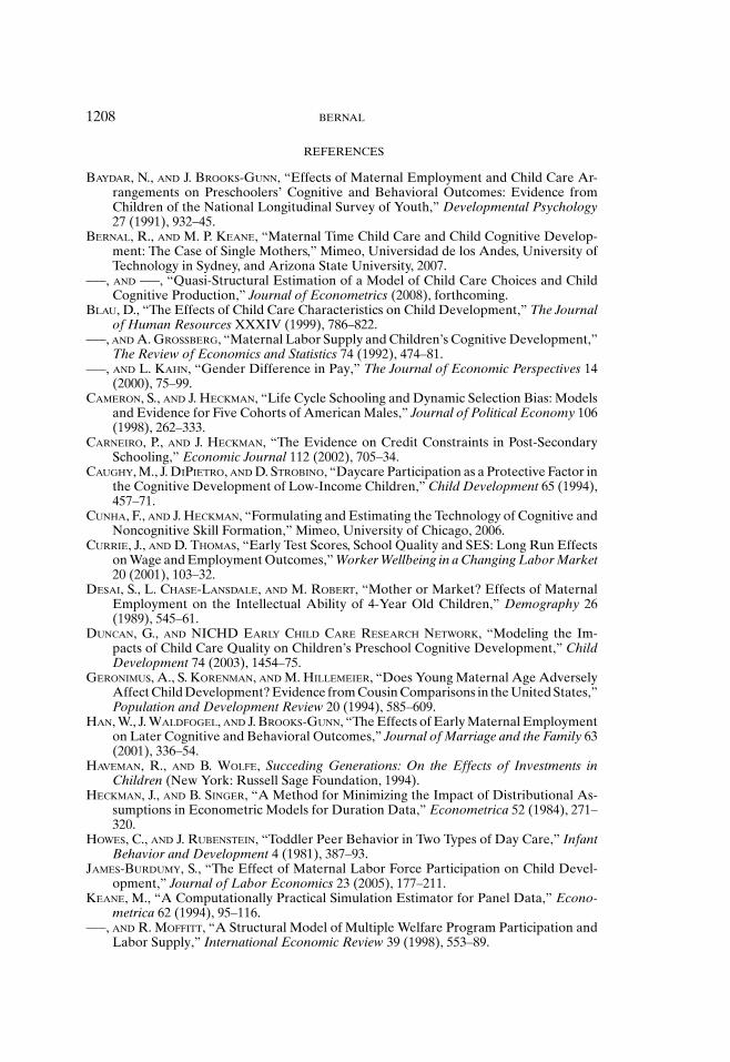
1208 BERNAL
REFERENCES
BAYDAR, N., AND J. BROOKS-GUNN, “Effects of Maternal Employment and Child Care Ar-rangements on Preschoolers’ Cognitive and Behavioral Outcomes: Evidence fromChildren of the National Longitudinal Survey of Youth,” Developmental Psychology27 (1991), 932–45.
BERNAL, R., AND M. P. KEANE, “Maternal Time Child Care and Child Cognitive Develop-ment: The Case of Single Mothers,” Mimeo, Universidad de los Andes, University ofTechnology in Sydney, and Arizona State University, 2007.
–––, AND –––, “Quasi-Structural Estimation of a Model of Child Care Choices and ChildCognitive Production,” Journal of Econometrics (2008), forthcoming.
BLAU, D., “The Effects of Child Care Characteristics on Child Development,” The Journalof Human Resources XXXIV (1999), 786–822.
–––, AND A. GROSSBERG, “Maternal Labor Supply and Children’s Cognitive Development,”The Review of Economics and Statistics 74 (1992), 474–81.
–––, AND L. KAHN, “Gender Difference in Pay,” The Journal of Economic Perspectives 14(2000), 75–99.
CAMERON, S., AND J. HECKMAN, “Life Cycle Schooling and Dynamic Selection Bias: Modelsand Evidence for Five Cohorts of American Males,” Journal of Political Economy 106(1998), 262–333.
CARNEIRO, P., AND J. HECKMAN, “The Evidence on Credit Constraints in Post-SecondarySchooling,” Economic Journal 112 (2002), 705–34.
CAUGHY, M., J. DIPIETRO, AND D. STROBINO, “Daycare Participation as a Protective Factor inthe Cognitive Development of Low-Income Children,” Child Development 65 (1994),457–71.
CUNHA, F., AND J. HECKMAN, “Formulating and Estimating the Technology of Cognitive andNoncognitive Skill Formation,” Mimeo, University of Chicago, 2006.
CURRIE, J., AND D. THOMAS, “Early Test Scores, School Quality and SES: Long Run Effectson Wage and Employment Outcomes,” Worker Wellbeing in a Changing Labor Market20 (2001), 103–32.
DESAI, S., L. CHASE-LANSDALE, AND M. ROBERT, “Mother or Market? Effects of MaternalEmployment on the Intellectual Ability of 4-Year Old Children,” Demography 26(1989), 545–61.
DUNCAN, G., AND NICHD EARLY CHILD CARE RESEARCH NETWORK, “Modeling the Im-pacts of Child Care Quality on Children’s Preschool Cognitive Development,” ChildDevelopment 74 (2003), 1454–75.
GERONIMUS, A., S. KORENMAN, AND M. HILLEMEIER, “Does Young Maternal Age AdverselyAffect Child Development? Evidence from Cousin Comparisons in the United States,”Population and Development Review 20 (1994), 585–609.
HAN, W., J. WALDFOGEL, AND J. BROOKS-GUNN, “The Effects of Early Maternal Employmenton Later Cognitive and Behavioral Outcomes,” Journal of Marriage and the Family 63(2001), 336–54.
HAVEMAN, R., AND B. WOLFE, Succeding Generations: On the Effects of Investments inChildren (New York: Russell Sage Foundation, 1994).
HECKMAN, J., AND B. SINGER, “A Method for Minimizing the Impact of Distributional As-sumptions in Econometric Models for Duration Data,” Econometrica 52 (1984), 271–320.
HOWES, C., AND J. RUBENSTEIN, “Toddler Peer Behavior in Two Types of Day Care,” InfantBehavior and Development 4 (1981), 387–93.
JAMES-BURDUMY, S., “The Effect of Maternal Labor Force Participation on Child Devel-opment,” Journal of Labor Economics 23 (2005), 177–211.
KEANE, M., “A Computationally Practical Simulation Estimator for Panel Data,” Econo-metrica 62 (1994), 95–116.
–––, AND R. MOFFITT, “A Structural Model of Multiple Welfare Program Participation andLabor Supply,” International Economic Review 39 (1998), 553–89.
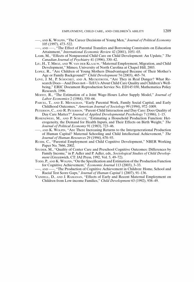
EMPLOYMENT, CHILD CARE, AND CHILDREN’S ABILITY 1209
–––, AND K. WOLPIN, “The Career Decisions of Young Men,” Journal of Political Economy105 (1997), 473–522.
–––, AND –––, “The Effect of Parental Transfers and Borrowing Constraints on EducationAttainment,” International Economic Review 42 (2001), 1051–03.
LAMB, M., “Effects of Nonparental Child Care on Child Development: An Update,” TheCanadian Journal of Psychiatry 41 (1996), 330–42.
LIU, H., T. MROZ, AND W. VAN DER KLAAUW, “Maternal Employment, Migration, and ChildDevelopment,” Mimeo, University of North Carolina at Chapel Hill, 2003.
LOPEZ, R., “Are Children of Young Mothers Disadvantaged Because of Their Mother’sAge or Family Background?” Child Development 74 (2003), 465–74.
LOVE, J. M., P. SCHOCHET, AND A. MECKSTROTH, “Are They in Real Danger? What Re-search Does—And Does not—Tell Us About Child Care Quality and Children’s Well-being,” ERIC Document Reproduction Service No. ED145 030, Mathematica PolicyResearch, 1996.
MOFFIT, R., “The Estimation of a Joint Wage-Hours Labor Supply Model,” Journal ofLabor Economics 2 (1984), 550–66.
PARCEL, T., AND E. MENAGHAN, “Early Parental Work, Family Social Capital, and EarlyChildhood Outcomes,” American Journal of Sociology 99 (1994), 972–1009.
PETERSON, C., AND R. PETERSON, “Parent-Child Interaction and Day Care: Does Quality ofDay Care Matter?” Journal of Applied Developmental Psychology 7 (1986), 1–15.
ROSENZWEIG, M., AND P. SCHULTZ, “Estimating a Household Production Function: Het-erogeneity, the Demand for Health Inputs, and Their Effects on Birth Weight,” TheJournal of Political Economy 91 (1983), 723–46.
–––, AND K. WOLPIN, “Are There Increasing Returns to the Intergenerational Productionof Human Capital? Maternal Schooling and Child Intellectual Achievement,” TheJournal of Human Resources 29 (1994), 670–93.
RUHM, C., “Parental Employment and Child Cognitive Development,” NBER WorkingPaper No. 7666, 2002.
STUDER, M., “Quality of Center Care and Preschool Cognitive Outcomes: Differences byFamily Income,” in P. Adler and P. Adler, eds., Sociological Studies of Child Develop-ment (Greenwich, CT: JAI Press, 1992, Vol. 5, 49–72).
TODD, P., AND K. WOLPIN, “On the Specification and Estimation of the Production Functionfor Cognitive Achievement,” Economic Journal 113 (2003), 3–33.
–––, AND –––, “The Production of Cognitive Achievement in Children: Home, School andRacial Test Score Gaps,” Journal of Human Capital 1 (2007), 91–136.
VANDELL, D., AND J. RAMANAN, “Effects of Early and Recent Maternal Employment onChildren from Low-income Families,” Child Development 63 (1992), 938–49.