the effect of private health insurance on medical care ... · the effect of private health...
TRANSCRIPT
The effect of private health insurance on medical careutilization and self-assessed health in Germany∗
Patrick Hullegie† and Tobias J. Klein‡
April 2010
Abstract
In Germany, employees are generally obliged to participate in the public health insurancesystem, where coverage is universal, co-payments and deductibles are moderate, and pre-mia are based on income. However, they may buy private insurance instead if their incomeexceeds the compulsory insurance threshold. Here, premia are based on age and health, in-dividuals may choose to what extent they are covered, and deductibles and co-payments arecommon. In this paper we estimate the effect of private insurance coverage on the numberof doctor visits, the number of nights spent in a hospital and self-assessed health. Variationin income around the compulsory insurance threshold provides a natural experiment that weexploit to control for selection into private insurance. We document that income is measuredwith error and suggest an approach to take this into account. We find negative effects ofprivate insurance coverage on the number of doctor visits, no effects on the number of nightsspent in a hospital, and positive effects on health.
JEL Classification: I11, I12, C31.Keywords: Private health insurance, medical care utilization, selection into insurance, naturalexperiment, regression discontinuity design, measurement error.
∗We would like to thank Jaap Abbring, Otilia Boldea, Katie Carman, Hans-Martin von Gaudecker, HendrikJürges, Peter Kooreman, Willard Manning, Martin Salm, one anonymous referee, and participants of the Netsparseminar (Tilburg University) and the 18th European Workshop on Econometrics and Health Economics for helpfulcomments.
†Netspar, CentER, Tilburg University. Address: Tilburg University, Department of Economics, PO Box 90153,5000 LE Tilburg, The Netherlands. E-Mail: [email protected].
‡Netspar, CentER, Tilburg University. Address: Tilburg University, Department of Econometrics and OR, POBox 90153, 5000 LE Tilburg, The Netherlands. E-Mail: [email protected].
1

1 Introduction
In Germany, employees are generally obliged to participate in the public health insurance system,
where coverage is universal, co-payments and deductibles are moderate, and premia are based on
income. However, they may buy private insurance instead if their income exceeds the so-called
compulsory insurance threshold.1 Here, premia are based on age and health, individuals may
choose to what extent they are covered, and deductibles and co-payments are common.2 These
differences in the incentive structure may affect both health behavior and the demand for medical
care. Once an individual faces an illness that requires medical treatment, the treatment costs for
a privately insured patient will be higher due to higher cost-sharing. For that reason, privately
insured patients have stronger incentives to invest in prevention to decrease the likelihood of
occurrence of an illness. Moreover, even in case the treatment provided to privately and publicly
insured patients is exactly the same, we would expect privately insured patients to be less inclined
to demand medical services.
An important difference affecting the supply of services is that for the same treatment the
compensation doctors receive for privately insured patients is, on average, 2.3 times as high as
the compensation for publicly insured patients (Walendzik et al., 2008). Therefore doctors have
an incentive to treat privately insured patients first, and more intensely, possibly providing better
treatment (Jürges, 2009). For example, waiting times for privately insured patients are lower on
average (Lungen et al., 2008). This may in turn affect the demand for medical care.
The combination of demand and supply side incentives determines whether the amount of
services consumed is higher or lower for privately insured individuals, and which effect insurance
type has on health. Ultimately, it is an empirical question whether more or less services are
consumed and how health depends on insurance status.
1About 90 percent of the German population is insured in the public health insurance system. Most remainingindividuals buy private insurance (Colombo & Tapay, 2004).
2In our data, 72 percent of the privately insured individuals who answered the respective question have insurancecontracts that involve deductibles or co-payments.
2

In this paper, we study the effect of being privately insured on the number of doctor visits,
the number of nights spent in a hospital and self-assessed health. We do not look at the effects
of specific insurance characteristics but look at the difference in usage between public and pri-
vate health insurance, keeping in mind that deductibles and co-payments are common features
of private insurance contracts. We do so by exploiting an unusual feature of the German public
health insurance system: as soon as income in the last year exceeds the so-called compulsory
insurance threshold individuals become eligible to opt out of the public health insurance system
and may buy private insurance instead. Random variation in income around this compulsory
insurance threshold generates a natural experiment that allows us to conduct a regression dis-
continuity (RD) analysis and estimate the effect of private insurance for those individuals who
buy private insurance once becoming eligible.3 This local average treatment effect is interesting
to policymakers considering to increase the compulsory insurance threshold, because this would
force exactly those individuals for whom we estimate the effect to return to the public system.
If in addition this local average treatment effect does not vary too much with income, so that
it is sufficiently close to the effect of private insurance on those who buy private insurance (the
treatment effect on the treated), then our results are informative about the effects of abandoning
the private system altogether.
We use survey data from the German Socio Economic Panel (GSOEP) for our analysis be-
cause German administrative data, that contain accurate income measures, do not contain health
related information. In the data, we find direct evidence for measurement error in income. More-
over, we find that there is a sizable number of individuals who, according to their reported in-
come, are not eligible to buy private insurance but at the same time report to be privately insured.
The methodological contribution in this paper is to model the measurement error in the so-called
3The RD approach has been suggested by Thistlethwaite and Campbell (1960) and has recently been developedby Hahn et al. (2001). They show that under relatively mild assumptions the RD method can be interpreted as alocal randomized experiment. This gives the results a strong internal validity. However, in general, a drawback isthat the effect is only estimated for a small subset of the population of interest/the population that a social planneris concerned with. See also Imbens and Lemieux (2008), Lee and Lemieux (2009) and Van der Klaauw (2009) forrecent discussions.
3

forcing variable, income in our case, within the RD framework. This then allows us to estimate
the effects of interest.
Controlling for selection into private insurance we find a significant negative effects of being
privately insured on the number of doctor visits for those individuals who visit the doctor at least
once in a three month period. At the same time, we find no significant effects on the number of
nights spent in a hospital, which can arguably be influenced less by the individual, and positive
effects on self-assessed health. This suggests that privately insured patients either receive better
or more intense treatment each time they see a doctor, or that they invest more in prevention.
The remainder of this paper is organized as follows. Section 2 and 3 discuss related re-
sults and the institutional details, respectively. In Section 4 we provide information on the data
and document that there is measurement error in income. Section 5 discusses the econometric
approach, emphasizing our approach to modeling measurement error. Results are presented in
Section 6, and a sensitivity analysis is performed in Section 7. Finally, Section 8 concludes.
2 Related Literature
The empirical literature on demand for health services dates at least back to the 1970s, when
the RAND Health Insurance Experiment (HIE) was conducted. One finding of this randomized
experiment is that the use of medical services responds negatively to changes in cost sharing,
with a stronger effect for outpatient care than for inpatient care (Newhouse, 1974; Manning et
al., 1987).
There are at least four studies for Germany that relate demand for medical services to insur-
ance type. They all use GSOEP data. Geil et al. (1997) estimate a count data model for hospital
visits on data from 1984-1989, 1992, and 1994. They find no relationship between insurance
coverage and the hospitalization decision. Riphahn et al. (2003) estimate a bivariate count data
model for physician and hospital visits. They use data from 1984 through 1995 and find that nei-
4

ther hospital nights nor doctor visits depend on the insurance type of the individual. Pohlmeier
and Ulrich (1995) and Jürges (2009) both estimate a negative binomial hurdle model. Pohlmeier
and Ulrich (1995) use data from 1985 and find that privately insured individuals are less likely
to contact a general practitioner but the number of visits once they do so is not significantly dif-
ferent from the one for publicly insured patients. Jürges (2009) uses data from 2002 and finds
that privately insured individuals are less likely to visit a doctor at all, but given that they do
the number of doctor visits is significantly larger than that of patients covered by public health
insurance. All four papers have in common that they do not control for selection into private
insurance.4
3 Institutional details
In Germany, about 90% of the population is publicly insured (Colombo & Tapay, 2004). Buying
public insurance is mandatory for dependent employees as long as their income does not exceed
the so-called compulsory insurance threshold. The public insurance premium equals a certain
percentage (nowadays about 14 percent that are equally shared between the employer and the
employee) of gross income up to the so-called contribution ceiling, and equal to it thereafter.5
Table 1 shows the contribution ceilings and the compulsory insurance thresholds by the year
in which the income was earned. To give an example of how the system works consider an indi-
vidual whose income, including all extra payments, in 2000 was 40,000 Euro. Then he is eligible
to buy private insurance in 2001 because his income exceeded 39,574 Euro, the compulsory in-
surance threshold. If his income stays the same in 2001, then he will have to join the public
insurance again in 2002 because the compulsory insurance threshold is 40,034 Euro for income
4The first two papers allow for random effects. Until recently both the theoretical and the empirical literature oninformational asymmetries focused on adverse selection and moral hazard (Akerlof, 1970; Rothschild & Stiglitz,1976; Arrow, 1963). However, Finkelstein and McGarry (2006) and Fang et al. (2008) point out that there might beadvantageous selection instead. Their explanation is that “good risks” select into insurance because they are morerisk averse and therefore value insurance more than “bad risks” do.
5See Jürges (2009) and the references therein for more details on this and the following discussion.
5
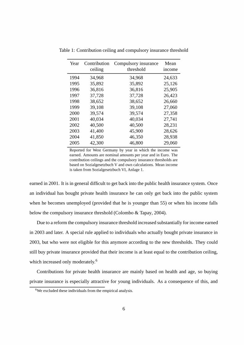
Table 1: Contribution ceiling and compulsory insurance threshold
Year Contribution Compulsory insurance Meanceiling threshold income
1994 34,968 34,968 24,6331995 35,892 35,892 25,1261996 36,816 36,816 25,9051997 37,728 37,728 26,4231998 38,652 38,652 26,6601999 39,108 39,108 27,0602000 39,574 39,574 27,3582001 40,034 40,034 27,7412002 40,500 40,500 28,2312003 41,400 45,900 28,6262004 41,850 46,350 28,9382005 42,300 46,800 29,060
Reported for West Germany by year in which the income wasearned. Amounts are nominal amounts per year and in Euro. Thecontribution ceilings and the compulsory insurance thresholds arebased on Sozialgesetzbuch V and own calculations. Mean incomeis taken from Sozialgesetzbuch VI, Anlage 1.
earned in 2001. It is in general difficult to get back into the public health insurance system. Once
an individual has bought private health insurance he can only get back into the public system
when he becomes unemployed (provided that he is younger than 55) or when his income falls
below the compulsory insurance threshold (Colombo & Tapay, 2004).
Due to a reform the compulsory insurance threshold increased substantially for income earned
in 2003 and later. A special rule applied to individuals who actually bought private insurance in
2003, but who were not eligible for this anymore according to the new thresholds. They could
still buy private insurance provided that their income is at least equal to the contribution ceiling,
which increased only moderately.6
Contributions for private health insurance are mainly based on health and age, so buying
private insurance is especially attractive for young individuals. As a consequence of this, and
6We excluded these individuals from the empirical analysis.
6
because of the fact that private insurers are allowed to reject individuals, the risk pool of the
private insurers is much better than in the public system.
Coverage is universal in the public system. Deductibles and co-payments are limited. Pri-
vately insured individuals can buy better care, e.g. treatment by the head doctor in a hospital
or a single room in a hospital, but this comes at a higher price. Deductibles and co-payments
are much more common, and many insurers offer a rebate if an individual did not use medical
services in the past calendar year. Unfortunately, specific characteristics of private insurance are
not recorded in our data.
At this point it is worth noticing that there is a feature called family insurance in the German
public health insurance system. A spouse is automatically insured if an individual is insured. For
this it is mandatory that the spouse is not full time self-employed and that the spouse does not earn
more than a rather low specified amount. If a married man is working then this system generates
incentives against working for his wife because then she would have to pay contributions which
amount to about 7 percent of her gross wage (the employer matches this and pays about the same
amount to the system). The family insurance feature does not exist for private health insurance
and therefore, individual insurance has to be purchased for each family member.
As already pointed out before insurance status has important consequences for the com-
pensation of doctors. For a given treatment the compensation doctors receive for privately in-
sured patients is, on average, 2.3 times as high as the compensation for publicly insured patients
(Walendzik et al., 2008). Furthermore, there is indirect evidence that doctors face strong time
constraints when treating patients. The consultation length for the average (publicly insured)
individual is very low in Germany.7 Deveugele et al. (2002, Table 4) compare the average con-
sultation length for general practitioners in six countries and find that with 7.6 minutes it is lowest
in Germany. It is highest in Switzerland, where it is equal to 15.6 minutes. Together with the
differences in the compensation this suggests that doctors dedicate more time to privately insured
7Recall that about 90 percent of the individuals are publicly insured. See footnote 1.
7
patients.
4 Data
The GSOEP we use in this study contain information at the individual level on medical care
utilization, self-assessed health, and background variables. We analyze data from West Germany
for the period from 1995 to 2006.8
Our sample is constructed such that eligibility to opt out of the public insurance system is
exclusively determined by income. Unemployed individuals who receive unemployment benefits
are required to be in the public health insurance system. For them there is no way to opt out
and therefore they are excluded. For self-employed, civil servants, soldiers, teachers in private
schools and students it is not mandatory to be in the public system, even if their income is below
the compulsory insurance threshold. Hence eligibility does not depend on income and therefore
they are excluded from the sample as well. Retired individuals, who receive a public pension,
are required to have public health insurance. They may opt out if insurance was not mandatory
in at least five years after the age of 55 and most of the time before that. Hence eligibility is
only weakly related to income and therefore they are excluded. Individuals of age 55 and older
are excluded for two reasons. First, because for them various ways to opt for (early) retirement
exist. Second, because for them it is difficult to get back into the public health insurance system.
Individuals under the age of 25 are excluded because a large fraction of them is covered by their
parents’ insurance.
To summarize, our study population consists of West German individuals, aged 25 to 55,
with a regular employment contract for whom eligibility to opt out of the public health insurance
8We do not use data before 1995 because the question on the number of doctor visits was phrased differently. Weuse data only up to 2006 because from 2007 onwards individuals had to earn more than the compulsory insurancethreshold in three consecutive years in order to be eligible to buy private insurance. East German individuals havebeen excluded because it turned out that for them, even when we control for measurement error in income, there isno jump in the probability to be privately insured when income is equal to the compulsory insurance threshold.
8
system is exclusively determined by income.
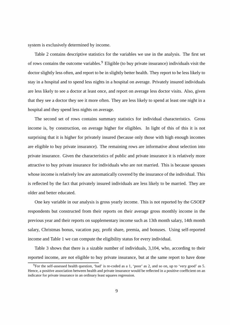
Table 2 contains descriptive statistics for the variables we use in the analysis. The first set
of rows contains the outcome variables.9 Eligible (to buy private insurance) individuals visit the
doctor slightly less often, and report to be in slightly better health. They report to be less likely to
stay in a hospital and to spend less nights in a hospital on average. Privately insured individuals
are less likely to see a doctor at least once, and report on average less doctor visits. Also, given
that they see a doctor they see it more often. They are less likely to spend at least one night in a
hospital and they spend less nights on average.
The second set of rows contains summary statistics for individual characteristics. Gross
income is, by construction, on average higher for eligibles. In light of this of this it is not
surprising that it is higher for privately insured (because only those with high enough incomes
are eligible to buy private insurance). The remaining rows are informative about selection into
private insurance. Given the characteristics of public and private insurance it is relatively more
attractive to buy private insurance for individuals who are not married. This is because spouses
whose income is relatively low are automatically covered by the insurance of the individual. This
is reflected by the fact that privately insured individuals are less likely to be married. They are
older and better educated.
One key variable in our analysis is gross yearly income. This is not reported by the GSOEP
respondents but constructed from their reports on their average gross monthly income in the
previous year and their reports on supplementary income such as 13th month salary, 14th month
salary, Christmas bonus, vacation pay, profit share, premia, and bonuses. Using self-reported
income and Table 1 we can compute the eligibility status for every individual.
Table 3 shows that there is a sizable number of individuals, 3,104, who, according to their
reported income, are not eligible to buy private insurance, but at the same report to have done
9For the self-assessed health question, ‘bad’ is re-coded as a 1, ‘poor’ as 2, and so on, up to ‘very good’ as 5.Hence, a positive association between health and private insurance would be reflected in a positive coefficient on anindicator for private insurance in an ordinary least squares regression.
9

Table 2: Descriptive statistics
(1) (2) (3) (4) (5)Public Private
Ineligible Eligible insurance insurance Total
At least 1 doctor visit 0.604 0.594 0.611 0.521 0.602- - - - -
Doctor visits given at least 1 visit 3.259 2.919 3.229 2.845 3.195(4.156) (3.365) (4.083) (3.304) (4.018)
Doctor visits 1.967 1.733 1.974 1.483 1.922(3.601) (2.963) (3.559) (2.776) (3.487)
At least 1 night in hospital 0.077 0.065 0.077 0.059 0.075- - - - -
Nights in hospital 0.827 0.655 0.822 0.551 0.793(4.934) (4.033) (4.812) (4.408) (4.772)
Self-assessed health 3.596 3.696 3.598 3.765 3.616(0.848) (0.790) (0.841) (0.789) (0.837)
Gross income 20,986.10 61,249.00 28,249.10 33,836.70 28,844.80(11,996.90) (27,755.60) (18,776.40) (43,628.00) (22,822.10)
Years of education 11.737 13.971 11.930 14.249 12.177(2.401) (2.929) (2.506) (3.038) (2.666)
Married 0.657 0.746 0.677 0.658 0.675- - - - -
Male 0.526 0.848 0.567 0.769 0.589- - - - -
Age 39.725 42.161 39.966 42.159 40.200(8.289) (7.206) (8.207) (7.334) (8.147)
N 40,821 9,900 45,313 5,408 50,721
Means and standard deviations (in parentheses). For binary variables only proportions are shown.Sample consists of dependent employees for whom eligibility to opt out of the public health insur-ance system is exclusively determined by income.
so. These 3,104 individuals constitute 57% of the individuals with private health insurance.
Misreporting insurance status or measurement error in income may both be valid explanations
for this.10
We consider it to be more plausible that income is measured with error because income is a
real number, and may thus be recalled with errors, whereas insurance status is more easily known
10There is an extensive literature on measurement error in income, see for example Bound et al. (2001) for asurvey. In order to study the accuracy of survey reports, they are typically compared with either employers’ oradministrative records. Some studies find that survey reports are highly correlated with record values, while othersfind much lower correlations. The mean of survey reports is found to be close to the mean of the record values. Thatis, under- or over-reporting, if present, is found to be moderate on average.
10
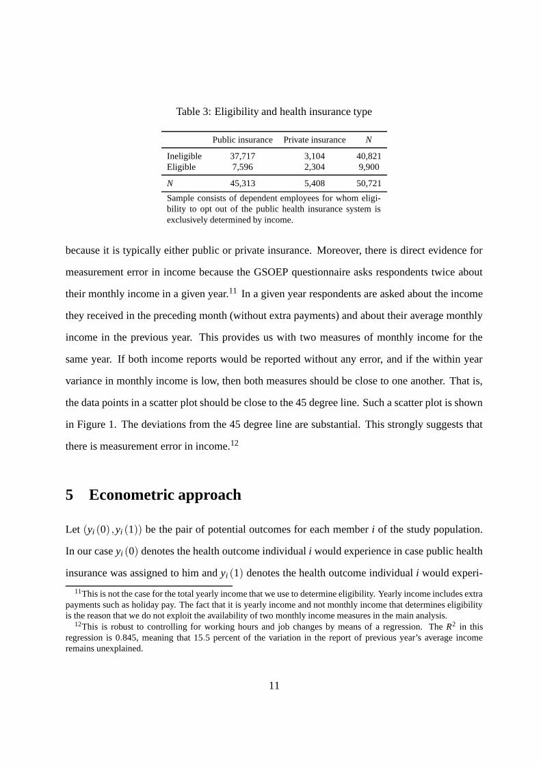
Table 3: Eligibility and health insurance type
Public insurance Private insurance N
Ineligible 37,717 3,104 40,821Eligible 7,596 2,304 9,900
N 45,313 5,408 50,721
Sample consists of dependent employees for whom eligi-bility to opt out of the public health insurance system isexclusively determined by income.
because it is typically either public or private insurance. Moreover, there is direct evidence for
measurement error in income because the GSOEP questionnaire asks respondents twice about
their monthly income in a given year.11 In a given year respondents are asked about the income
they received in the preceding month (without extra payments) and about their average monthly
income in the previous year. This provides us with two measures of monthly income for the
same year. If both income reports would be reported without any error, and if the within year
variance in monthly income is low, then both measures should be close to one another. That is,
the data points in a scatter plot should be close to the 45 degree line. Such a scatter plot is shown
in Figure 1. The deviations from the 45 degree line are substantial. This strongly suggests that
there is measurement error in income.12
5 Econometric approach
Let (yi (0) ,yi (1)) be the pair of potential outcomes for each member i of the study population.
In our case yi (0) denotes the health outcome individual i would experience in case public health
insurance was assigned to him and yi (1) denotes the health outcome individual i would experi-
11This is not the case for the total yearly income that we use to determine eligibility. Yearly income includes extrapayments such as holiday pay. The fact that it is yearly income and not monthly income that determines eligibilityis the reason that we do not exploit the availability of two monthly income measures in the main analysis.
12This is robust to controlling for working hours and job changes by means of a regression. The R2 in thisregression is 0.845, meaning that 15.5 percent of the variation in the report of previous year’s average incomeremains unexplained.
11

Figure 1: Joint distribution of the two income measures
050
0010
000
1500
0La
st y
ear’s
rep
ort o
f las
t yea
r’s m
onth
ly in
com
e
0 5000 10000 15000Current year’s report of last year’s monthly income
Sample consists of dependent employees for whom eligi-bility to opt out of the public health insurance system isexclusively determined by income. For this figure we useonly income reports below 15,000 Euro per month.
ence if private health insurance was assigned. That is, we consider private health insurance to be
the “treatment.”
An individual is eligible to buy private health insurance instead of public insurance if his
income in the previous year exceeded the respective compulsory insurance threshold. That is, an
individual is eligible when z∗i ≥ 0, where z∗i denotes the difference between income earned in the
previous year and the corresponding compulsory insurance threshold. Buying private insurance
is voluntary for eligible individuals so that some will buy it while others will not.
Hahn et al. (2001) show that two assumptions are needed to identify a local average treatment
effect. First, the mean value of yi (0) conditional on z∗i is a continuous function of z∗i at z∗i =
0. This assumption holds if the mean health outcome would be a smooth function in income
around the compulsory insurance threshold once public insurance was exogenously assigned to
everybody. This is highly plausible. Second, we assume that the decision to buy private insurance
12
is monotone in eligibility. This is the monotonicity condition of Imbens and Angrist (1994). It
holds by construction because ineligibles cannot buy private insurance. Under these assumptions
the average treatment effect for those individuals that would buy private health insurance when
becoming eligible is given by
∆LATE ≡ E(yi (1)− yi (0) |pi = 1,z∗i = 0) =E(yi|z∗i = 0+)−E(yi|z∗i = 0−)
E(
pi|z∗i = 0+) , (1)
where yi is the observed health outcome, pi is an indicator of private insurance, E(·|z∗i = 0+) ≡
limδ↓0 E(·|z∗i = δ ), and E(·|z∗i = 0−) ≡ limδ↑0 E(·|z∗i = δ ). This effect is of particular interest
because it is directly related to the question what the effect of requiring all individuals to buy
public insurance would be.
Measurement error in income leads to misclassification of eligibility. Importantly, this mis-
classification is not independent of the true underlying income because if the true underlying
income is below (above) the compulsory insurance threshold the classification error can only
be that the individual is (not) eligible to buy private insurance. This precludes the use of an
instrumental variables approach to estimating the unknown quantities in the numerator and de-
nominator in equation (1).
The effect of the measurement error in income on estimates of these quantities is that no
discontinuity in reported income is observed at the threshold (Battistin et al., 2009). In Figure
2, the dots are fractions of privately insured individuals which we plot against the difference
in income and the compulsory insurance threshold. The figure shows that these fractions are
not zero if reported income is below the compulsory insurance threshold, i.e. if the value of
the difference on the horizontal axis is negative, and that indeed there is no discontinuity in the
fraction of privately insured at the threshold.
Towards estimating the local average treatment effect in the presence of measurement error
we now develop an expression for the probability to be privately insured, which is equal to the
13
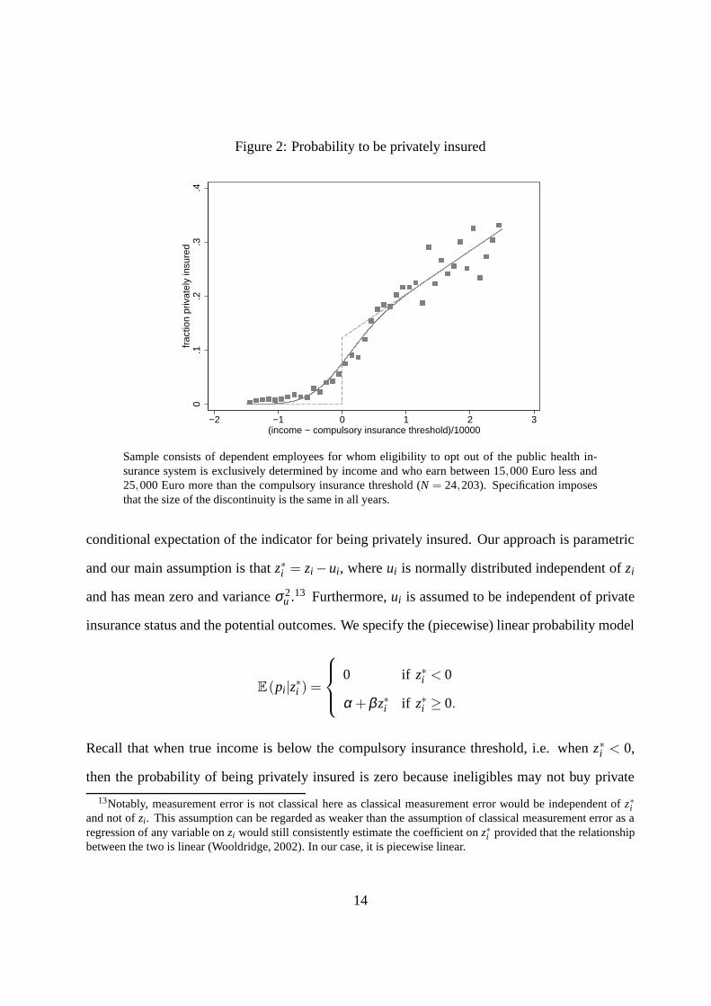
Figure 2: Probability to be privately insured
0.1
.2.3
.4fr
actio
n pr
ivat
ely
insu
red
−2 −1 0 1 2 3(income − compulsory insurance threshold)/10000
Sample consists of dependent employees for whom eligibility to opt out of the public health in-surance system is exclusively determined by income and who earn between 15,000 Euro less and25,000 Euro more than the compulsory insurance threshold (N = 24,203). Specification imposesthat the size of the discontinuity is the same in all years.
conditional expectation of the indicator for being privately insured. Our approach is parametric
and our main assumption is that z∗i = zi − ui, where ui is normally distributed independent of zi
and has mean zero and variance σ 2u .13 Furthermore, ui is assumed to be independent of private
insurance status and the potential outcomes. We specify the (piecewise) linear probability model
E(pi|z∗i ) =
0 if z∗i < 0
α +β z∗i if z∗i ≥ 0.
Recall that when true income is below the compulsory insurance threshold, i.e. when z∗i < 0,
then the probability of being privately insured is zero because ineligibles may not buy private
13Notably, measurement error is not classical here as classical measurement error would be independent of z∗iand not of zi. This assumption can be regarded as weaker than the assumption of classical measurement error as aregression of any variable on zi would still consistently estimate the coefficient on z∗i provided that the relationshipbetween the two is linear (Wooldridge, 2002). In our case, it is piecewise linear.
14

insurance. Conversely, when true income exceeds the compulsory insurance threshold, i.e. when
z∗i ≥ 0, individuals may buy private insurance.
We show in Appendix A that under these assumptions
E(pi|zi) = Φ(
zi
σu
)
·
α +β zi +βσu
φ(
ziσu
)
Φ(
ziσu
)
, (2)
where Φ(·) is the standard normal cumulative distribution function and φ (·) is the standard nor-
mal probability density function. Notably, this is the prediction for the relationship between the
probability to be privately insured and the difference between reported income and the compul-
sory insurance threshold (zi). The solid line in Figure 2 shows the estimated relationship for
our data when we pool data across all years. The dots are sample fractions of privately insured.
Comparing them to the solid line shows that the fit is reasonably good. Finally, the dashed line in
this figure is the underlying relationship between the probability to be privately insured and the
difference between actual (measured without error) yearly income and the compulsory insurance
threshold (z∗i ).
A similar expression can be obtained for E(yi|zi). This involves specifying different linear
functions to the left and right of the discontinuity,
E(yi|z∗i ) =
α0 +β0z∗i if z∗i < 0
α1 +β1z∗i if z∗i ≥ 0,
15

so that, under our assumptions,
E(yi|zi) =
(
1−Φ(
zi
σu
))
α0 +β0zi−β0σu
φ(
ziσu
)
1−Φ(
ziσu
)
+Φ(
zi
σu
)
α1 +β1zi +β1σu
φ(
ziσu
)
Φ(
ziσu
)
. (3)
The parameters for both E(pi|zi) and E(yi|zi) will be jointly estimated using the feasible
generalized nonlinear least squares estimator for nonlinear systems of equations. We then calcu-
late the local average treatment effect from these parameter estimates. For this observe that α ,
α0, and α1 are equal to E(pi|z∗i = 0+), E(yi|z∗i = 0−), and E(yi|z∗i = 0+), respectively. Hence,
it follows from equation (1) that the local average treatment effect is given by
∆LATE =α1 −α0
α. (4)
6 Results
We jointly estimate the equation for the probability to be privately insured conditional on reported
income, equation (2), and the equation for medical care utilization conditional on reported in-
come, equation (3). Throughout, we allow the probability to be privately insured to have year
specific jumps at the compulsory insurance threshold. This is reasonable since the compulsory
insurance threshold changed over time (see Table 1). We impose that the local average treatment
effect is the same in all years, i.e. we impose that ∆LATE , our parameter of main interest, is
independent of z∗i . Then, it follows from equation (4) that we can replace α1 by α0 +∆LATE ·α .
Notice that the size of both the numerator and the denominator in equation (1) is still allowed to
vary across years, but we impose that the relative change in both is the same. Finally, we impose
16
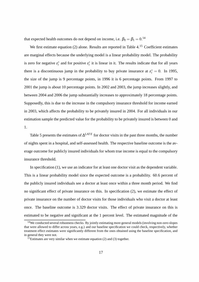
that expected health outcomes do not depend on income, i.e. β0 = β1 = 0.14
We first estimate equation (2) alone. Results are reported in Table 4.15 Coefficient estimates
are marginal effects because the underlying model is a linear probability model. The probability
is zero for negative z∗i and for positive z∗i it is linear in it. The results indicate that for all years
there is a discontinuous jump in the probability to buy private insurance at z∗i = 0. In 1995,
the size of the jump is 9 percentage points, in 1996 it is 6 percentage points. From 1997 to
2001 the jump is about 10 percentage points. In 2002 and 2003, the jump increases slightly, and
between 2004 and 2006 the jump substantially increases to approximately 18 percentage points.
Supposedly, this is due to the increase in the compulsory insurance threshold for income earned
in 2003, which affects the probability to be privately insured in 2004. For all individuals in our
estimation sample the predicted value for the probability to be privately insured is between 0 and
1.
Table 5 presents the estimates of ∆LATE for doctor visits in the past three months, the number
of nights spent in a hospital, and self-assessed health. The respective baseline outcome is the av-
erage outcome for publicly insured individuals for whom true income is equal to the compulsory
insurance threshold.
In specification (1), we use an indicator for at least one doctor visit as the dependent variable.
This is a linear probability model since the expected outcome is a probability. 60.6 percent of
the publicly insured individuals see a doctor at least once within a three month period. We find
no significant effect of private insurance on this. In specification (2), we estimate the effect of
private insurance on the number of doctor visits for those individuals who visit a doctor at least
once. The baseline outcome is 3.329 doctor visits. The effect of private insurance on this is
estimated to be negative and significant at the 1 percent level. The estimated magnitude of the
14We conducted several robustness checks. By jointly estimating more general models (involving non-zero slopesthat were allowed to differ across years, e.g.) and our baseline specification we could check, respectively, whethertreatment effect estimates were significantly different from the ones obtained using the baseline specification, andin general they were not.
15Estimates are very similar when we estimate equation (2) and (3) together.
17

Table 4: Probability to be privately insured
(Gross income - threshold)/10000 0.075***(0.005)
Discontinuity 1995 0.089***(0.013)
Discontinuity 1996 0.064***(0.013)
Discontinuity 1997 0.099**(0.041)
Discontinuity 1998 0.098***(0.014)
Discontinuity 1999 0.107***(0.013)
Discontinuity 2000 0.101***(0.010)
Discontinuity 2001 0.109***(0.011)
Discontinuity 2002 0.132***(0.010)
Discontinuity 2003 0.114***(0.010)
Discontinuity 2004 0.193***(0.011)
Discontinuity 2005 0.191***(0.012)
Discontinuity 2006 0.178***(0.011)
σu 0.463***(0.034)
R2 0.184N 24,203
Standard errors are clustered at the individual level andshown in parentheses. ∗,∗∗,∗∗∗ denote significance at the10, 5, and 1 % level, respectively. Sample consists of de-pendent employees for whom eligibility to opt out of thepublic health insurance system is exclusively determined byincome and who earn between 15,000 Euro less and 25,000Euro more than the compulsory insurance threshold.
effect, however, seems to be too big. Nevertheless, the upper limit of the 95 percent confidence
interval is −1.893, which seems more reasonable in terms of the magnitude. Specification (3) is
18

Table 5: Baseline specification
(1) (2) (3) (4) (5) (6)At least one Doctor visits Doctor visits At least one night Nights in Self-assesseddoctor visits for subsample in hospital hospital health
∆LATE -0.079 -3.746*** -2.137*** -0.063* -1.084* 0.449***(0.076) (0.945) (0.546) (0.035) (0.572) (0.160)
Baseline outcome 0.606*** 3.329*** 2.013*** 0.074*** 0.783*** 3.614***(0.005) (0.054) (0.039) (0.002) (0.039) (0.011)
N 24,203 14,579 24,203 24,203 24,203 24,203
Standard errors are clustered at the individual level and shown in parentheses. ∗,∗∗,∗ ∗ ∗ denote significance at the 10, 5, and 1 % level,respectively. Sample consists of dependent employees for whom eligibility to opt out of the public health insurance system is exclusivelydetermined by income and who earn between 15,000 Euro less and 25,000 Euro more than the compulsory insurance threshold.
for the number of doctor visits in the entire sample. This is a combination of the two effects we
discussed above. The mean baseline outcome is estimated to be 2.013. The estimated effect is
negative and significant at the 1 percent level, but again the magnitude of the point estimate is
too big as it exceeds the baseline in terms of the magnitude. However, the upper end of the 95
percent confidence interval is −1.067, which seems more reasonable than the point estimate.
Manning, Morris, and Newhouse (1981) argue that the decision to visit a doctor at all, the
so-called contact decision, is made by the individual, whereas the number of visits is mainly
determined by the doctor. However, it could also be that the patient and the doctor jointly deter-
mine the number of visits, or that fewer visits are needed for privately insured patients because
they have invested in prevention. Furthermore, it could be that privately insured patients are
treated more intensely so that less doctor visits are necessary. This is sensible because doctors
are paid based on the number of treatments, not on the number of visits itself, and receive a
higher compensation when they treat privately insured patients. They are time constraint and
may thus focus on treating privately insured patients first (Lungen et al., 2008; Jürges, 2009),
while spending relatively little time on publicly insured patients (Deveugele et al., 2002).
In specification (4) we use an indicator for at least one night spent in a hospital as the de-
pendent variable. This is also a linear probability model. 7.4 percent of the publicly insured
19

spend at least one night in a hospital. The results indicate that there is no significant effect of
private insurance on this (at the 5 percent level). Specification (5) is for the number of nights
spent in a hospital and also here we find no significant effect of private insurance (also at the 5
percent level). These findings for hospital nights are in line with those of Geil et al. (1997) and
Riphahn et al. (2003), and is intuitively plausible as the number of nights spent in a hospital can
be influenced less by the individual than the the number of doctor visits is. Finally, we find that
private insurance has a positive effect on health. The size of the effect seems big, but the lower
end of the 95 percent interval is given by 0.136, which seems reasonable.
7 Sensitivity analysis
Generally, we do not have to control for covariates when performing an RD analysis unless the
distribution of the covariates changes when we move from the left to the right of the discontinuity
(Imbens & Lemieux, 2008). The measurement error in the forcing variable, however, prevents us
from performing the usual tests. However, it is still feasible to perform the analysis incorporating
a dependence of the baseline outcome and the probability to be privately insured on additional
covariates. Table 6 reports the results. They are similar to our baseline results.
Some of the studies that use GSOEP data additionally condition on health when estimat-
ing the relationship between private insurance coverage and the health outcomes (Jürges, 2009,
e.g.). For two reasons we consider it reasonable to condition on previous period’s health instead
of current health. First, one of the outcomes in this study is current period’s health so that con-
ditioning on current health is not sensible, at least for this outcome. Second, current period’s
health is likely to be endogenous. We condition on previous period’s health by re-estimating the
model for individuals who report in the previous period that their health is “satisfactory”. Table
7 contains the results.16
16These results were obtained using a two-step procedure to achieve convergence. This procedure is described inthe Online Appendix.
20
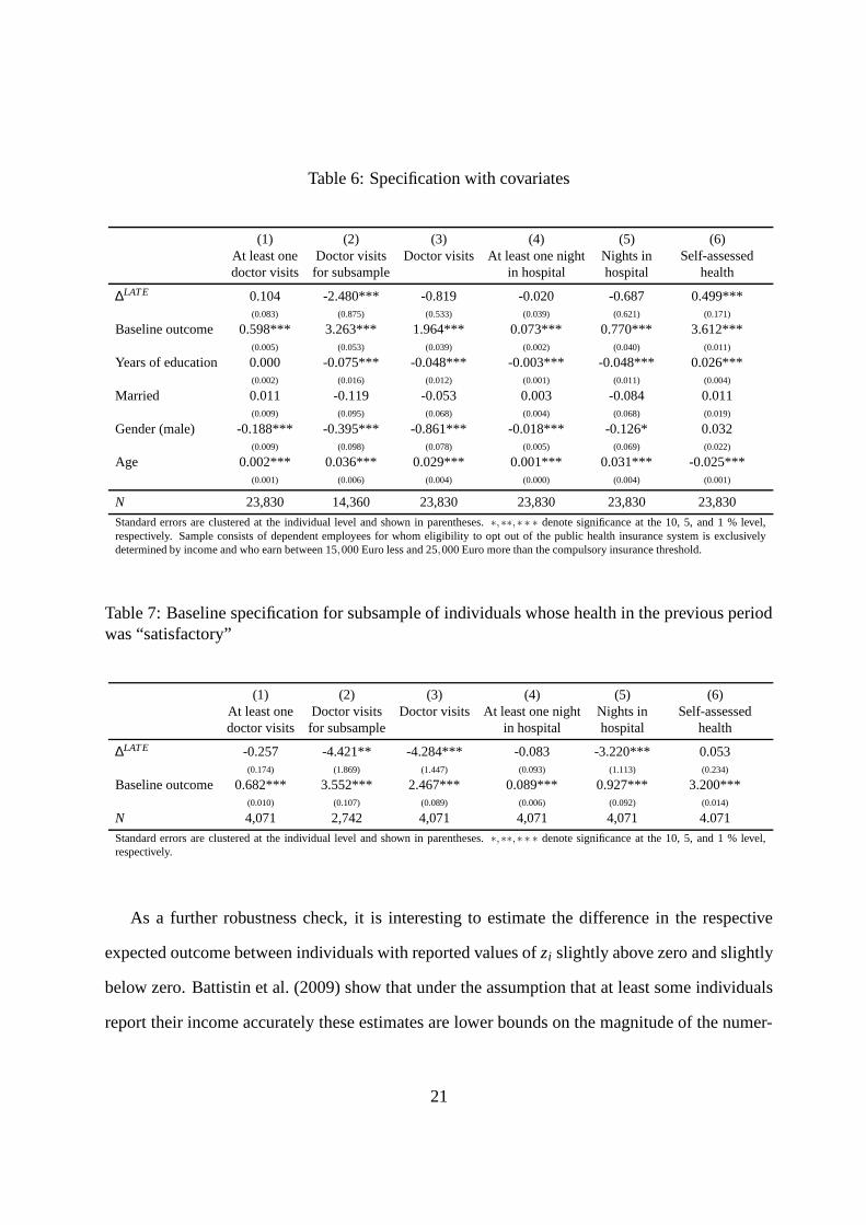
Table 6: Specification with covariates
(1) (2) (3) (4) (5) (6)At least one Doctor visits Doctor visits At least one night Nights in Self-assesseddoctor visits for subsample in hospital hospital health
∆LATE 0.104 -2.480*** -0.819 -0.020 -0.687 0.499***(0.083) (0.875) (0.533) (0.039) (0.621) (0.171)
Baseline outcome 0.598*** 3.263*** 1.964*** 0.073*** 0.770*** 3.612***(0.005) (0.053) (0.039) (0.002) (0.040) (0.011)
Years of education 0.000 -0.075*** -0.048*** -0.003*** -0.048*** 0.026***(0.002) (0.016) (0.012) (0.001) (0.011) (0.004)
Married 0.011 -0.119 -0.053 0.003 -0.084 0.011(0.009) (0.095) (0.068) (0.004) (0.068) (0.019)
Gender (male) -0.188*** -0.395*** -0.861*** -0.018*** -0.126* 0.032(0.009) (0.098) (0.078) (0.005) (0.069) (0.022)
Age 0.002*** 0.036*** 0.029*** 0.001*** 0.031*** -0.025***(0.001) (0.006) (0.004) (0.000) (0.004) (0.001)
N 23,830 14,360 23,830 23,830 23,830 23,830
Standard errors are clustered at the individual level and shown in parentheses. ∗,∗∗,∗ ∗ ∗ denote significance at the 10, 5, and 1 % level,respectively. Sample consists of dependent employees for whom eligibility to opt out of the public health insurance system is exclusivelydetermined by income and who earn between 15,000 Euro less and 25,000 Euro more than the compulsory insurance threshold.
Table 7: Baseline specification for subsample of individuals whose health in the previous periodwas “satisfactory”
(1) (2) (3) (4) (5) (6)At least one Doctor visits Doctor visits At least one night Nights in Self-assesseddoctor visits for subsample in hospital hospital health
∆LATE -0.257 -4.421** -4.284*** -0.083 -3.220*** 0.053(0.174) (1.869) (1.447) (0.093) (1.113) (0.234)
Baseline outcome 0.682*** 3.552*** 2.467*** 0.089*** 0.927*** 3.200***(0.010) (0.107) (0.089) (0.006) (0.092) (0.014)
N 4,071 2,742 4,071 4,071 4,071 4.071
Standard errors are clustered at the individual level and shown in parentheses. ∗,∗∗,∗ ∗ ∗ denote significance at the 10, 5, and 1 % level,respectively.
As a further robustness check, it is interesting to estimate the difference in the respective
expected outcome between individuals with reported values of zi slightly above zero and slightly
below zero. Battistin et al. (2009) show that under the assumption that at least some individuals
report their income accurately these estimates are lower bounds on the magnitude of the numer-
21
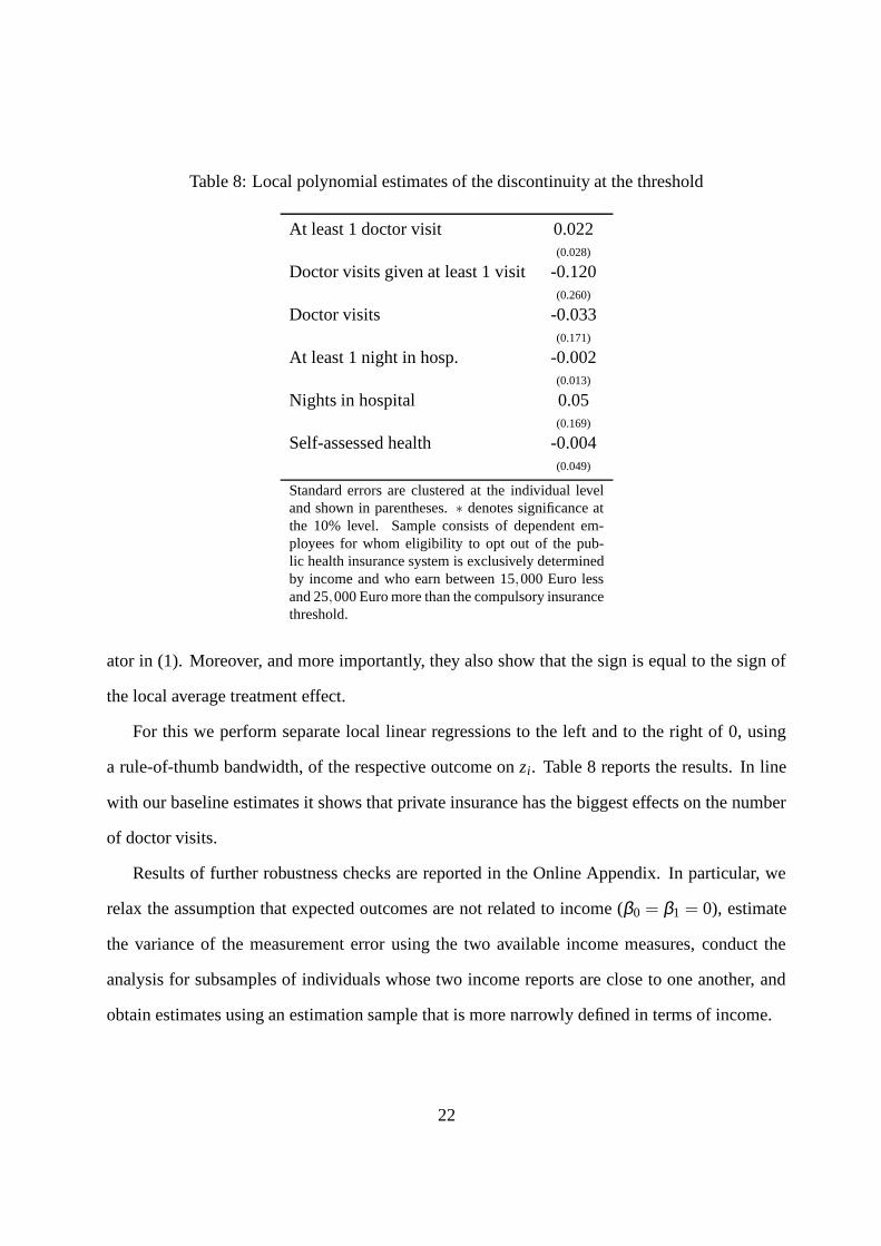
Table 8: Local polynomial estimates of the discontinuity at the threshold
At least 1 doctor visit 0.022(0.028)
Doctor visits given at least 1 visit -0.120(0.260)
Doctor visits -0.033(0.171)
At least 1 night in hosp. -0.002(0.013)
Nights in hospital 0.05(0.169)
Self-assessed health -0.004(0.049)
Standard errors are clustered at the individual leveland shown in parentheses. ∗ denotes significance atthe 10% level. Sample consists of dependent em-ployees for whom eligibility to opt out of the pub-lic health insurance system is exclusively determinedby income and who earn between 15,000 Euro lessand 25,000 Euro more than the compulsory insurancethreshold.
ator in (1). Moreover, and more importantly, they also show that the sign is equal to the sign of
the local average treatment effect.
For this we perform separate local linear regressions to the left and to the right of 0, using
a rule-of-thumb bandwidth, of the respective outcome on zi. Table 8 reports the results. In line
with our baseline estimates it shows that private insurance has the biggest effects on the number
of doctor visits.
Results of further robustness checks are reported in the Online Appendix. In particular, we
relax the assumption that expected outcomes are not related to income (β0 = β1 = 0), estimate
the variance of the measurement error using the two available income measures, conduct the
analysis for subsamples of individuals whose two income reports are close to one another, and
obtain estimates using an estimation sample that is more narrowly defined in terms of income.
22
8 Conclusions
In this paper we estimate the effect of private health insurance on the number of doctor visits, the
number of nights spent in a hospital, and self-assessed health in Germany. Variation in income
around the compulsory insurance threshold generates a natural experiment which allows us to
control for selection into private insurance and estimate respective average treatment effects for
individuals who buy private insurance once they become eligible by earning enough.
We show that it is important to account for measurement error in income and suggest a way to
do so. We find a significant negative effect of private insurance on the number of doctor visits for
those individuals who see the doctor at least once. At the same time, we find no effect of private
health insurance on the number of nights spent in a hospital, and a positive effect on self-assessed
health. This suggests that private health insurance either has a positive effect on investment in
prevention, because of the monetary incentives provided to the insured, or that privately insured
patients receive more intense or better treatment each time they visit a doctor.
Appendix A: Derivations
In this appendix we derive an expression for E(pi|z∗i ) = Pr (pi = 1|z∗i ). Recall that z∗i = zi − ui,
where ui is normally distributed with mean 0 and variance σ 2u , statistically independent of zi, pi
and the potential outcomes. For z∗i < 0 we have that E(pi|z∗i ) = 0 by definition. For z∗i ≥ 0 we
specify E(pi|z∗i ) to be a linear function in z∗i , a linear probability model. That is,
E(pi|z∗i ) =
0 if z∗i < 0
α +β z∗i if z∗i ≥ 0.
23

By the law of total probability,
E(pi|zi) = Pr (z∗i < 0|zi) ·0+Pr(z∗i ≥ 0|zi) ·E(pi|zi,z∗i ≥ 0) .
The assumptions about the measurement error imply that this is equivalent to
E(pi|zi) = Pr(ui ≤ zi) · (α +βE(zi−ui|zi,ui ≤ zi)) . (5)
Recall that if v is standard normally distributed then E(v|v < c) =−φ (c)/Φ(c), which is known
as the inverse Mills ratio, where Φ(·) and φ(·) denote the standard normal cumulative distribu-
tion function and the probability density function, respectively. Using this equation (5) can be
rewritten as
E(pi|zi) = Φ(
zi
σu
)
·
α +β zi +βσu
φ(
ziσu
)
Φ(
ziσu
)
.
ReferencesAkerlof, G. (1970). The market for ‘lemons’: Quality uncertainty and the market mechanism.
Quarterly Journal of Economics, 84, 488-500.Arrow, K. (1963). Uncertainty and the welfare economics of medical care. American Economic
Review, 53, 941-973.Battistin, E., Brugiavini, A., Rettore, E., & Weber, G. (2009). The retirement consumption
puzzle: Evidence from a regression discontinuity approach. American Economic Review,2209 - 2226.
Bound, J., Brown, C., & Mathiowetz, N. (2001). Measurement error in survey data. In J. Heck-man & E. Leamer (Eds.), Handbook of Econometrics, volume 5 (p. 3705 - 3843). ElsevierScience.
Colombo, F., & Tapay, N. (2004). Private health insurance in OECD countries: The benefitsand costs for individuals and health systems. OECD Health Working Paper No 15.
Deveugele, M., Derese, A., van den Brink-Muinen, A., Bensing, J., & De Maeseneer, J. (2002).Consultation length in general practice: Cross sectional study in six European countries.British Medical Journal, 325, 472-477.
Fang, H., Keane, M., & Silverman, D. (2008). Sources of advantageous selection: Evidencefrom the Medigap insurance market. Journal of Political Economy, 116, 303 - 350.
24
Finkelstein, A., & McGarry, K. (2006). Multiple demensions of private information: Evidencefrom the long-term care insurance market. American Economic Review, 96, 938 - 958.
Geil, P., Million, A., Rotte, R., & Zimmerman, K. (1997). Economic incentives and hospitaliza-tion in Germany. Journal of Applied Econometrics, 12, 295-311.
Hahn, J., Todd, P., & Van der Klaauw, W. (2001). Identification and estimation of treatmenteffects with a regression discontinuity design. Econometrica, 69, 201 - 209.
Imbens, G., & Angrist, J. (1994). Identification and estimation of local average treatment effects.Econometrica, 62, 467-475.
Imbens, G., & Lemieux, T. (2008). Regression discontinuity designs: A guide to pratice. Journalof Econometrics, 142, 615 - 635.
Jürges, H. (2009). Health insurance status and physician behavior in Germany. In Schmoller’sJahrbuch (Vol. 129, p. 297 - 307).
Lee, D., & Lemieux, T. (2009). Regression discontinuity designs in economics. Working PaperNo. 14723 NBER.
Lungen, M., Stollenwerk, B., Messner, P., Lauterbach, K. W., & Gerber, A. (2008). Waitingtimes for elective treatments according to insurance status: A randomized empirical studyin Germany. International Journal for Equity in Health, 7(1), 1-7.
Manning, W., Morris, C., & Newhouse, J. (1981). A two-part model of the demand for medicalcare: Preliminary results from the health insurance study. In J. van der Gaag & M. Perlman(Eds.), Economics and health economics. Amsterdam: North Holland.
Manning, W., Newhouse, J., Duan, N., Keeler, E., Leibowitz, A., & Marquis, M. (1987). Healthinsurance and the demand for medical care: Evidence from a randomized experiment.American Economic Review, 77, 251 - 277.
Newhouse, J. (1974). A design for a health insurance experiment. Inquiry, 11, 5 - 27.Pohlmeier, W., & Ulrich, V. (1995). An econometric model of the two-part decisionmaking
process in the demand for health care. Journal of Human Resources, 30(2), 339-361.Riphahn, R., Wambach, A., & Million, A. (2003). Incentive effects in the demand for health
care: A bivariate panel count data estimation. Journal of Applied Econometrics, 18, 387 -405.
Rothschild, M., & Stiglitz, J. (1976). Equilibrium in competitive insurance markets: An essay inthe economics of incomplete information. Quarterly Journal of Economics, 90, 624-649.
Thistlethwaite, D., & Campbell, D. (1960). Regression discontinuity analysis: An alternative tothe ex post facto experiment. Journal of Educational Psychology, 51, 309 - 317.
Van der Klaauw, W. (2009). Regression discontinuity anlaysis: A survey of recent developmentsin economics. Labour, 22, 219 - 245.
Walendzik, A., Gress, S., Manouguian, M., & Wasem, J. (2008). Vergütungsunterschiedeim ärztlichen Bereich zwischen PKV und GKV auf Basis des standardisierten Leis-tungsniveaus der GKV und Modelle der Vergütungsangleichung. Diskussionsbeitrag No.165, University of Duisburg-Essen.
Wooldridge, J. M. (2002). Econometric analysis of cross section and panel data. Cambridge,MA: MIT Press.
25