VT

T T

EC

HN

OL

OG

Y 1

27

T

he

effe

ct o

f stress sta

te o

n g

rou

nd

wa

ter fl

ow

in b

ed

roc

k

ISBN 978-951-38-8054-5 (URL: http://www.vtt.fi/publications/index.jsp)ISSN-L 2242-1211ISSN 2242-122X (Online)

The effect of stress state on groundwater flow in bedrock Simulations of in situ experiments

The effect of stress state on groundwater flow in bedrockSimulations of in situ experiments

Karita Kajanto

•VISIONS•S

CIE

NC

E•T

ECHNOLOGY•R

ES

EA

RC

HHIGHLIGHTS

127

VTT TECHNOLOGY 127

The effect of stress state ongroundwater flow in bedrockSimulations of in situ experiments

Karita Kajanto

3

The effect of stress state on groundwater flow in bedrockSimulations of in situ experimentsJännitystilan vaikutus pohjaveden virtaukseen kallioperässä. Paikkatutkimustulosten mallinnusta.Karita Kajanto. Espoo 2013. VTT Technology 127. 59 p.

AbstractThe effect of the stress state on the permeability of bedrock for groundwater was studied bysimulating an in situ experiment. Previous studies show that the dependency of permeability onstress can have a significant effect on flow. Several models have been developed, but little hasbeen done in order to develop models suitable for in situ applications, such as the deep under-ground repositories for spent nuclear fuel. In repositories, stress state evolves during the longtime period considered in safety assessment. The effect of the changing flow pattern, due to theevolving stress, has to be estimated for, e.g., radionuclide transport calculations.

Previous work done in the field was reviewed, existing relations between stress and permea-bility were analysed, and suitable relations were selected for the modelling cases. Rock masspermeability and discrete fracture permeability were treated separately. One new empiricalmodel for fracture permeability was presented and three models were further developed to bemore suitable for 3-D implementation. Simulations followed in situ experiments conducted inÄspö Hard Rock Laboratory. The modelling geometry was constructed based on the experi-mental setup and the fracture information from the location. The overall stress state in the areawas known and the effect of the measurement tunnel and boreholes was computed. The stressstate was used to compute the groundwater flow, and the applicability of the chosen models forin situ modelling was analysed. COMSOL Multiphysics was used as the tool for the simulations.

The simulation results followed the measurements reasonably well, but differences werefound with one model. The results show that differences between most of the models were rela-tively small if inflow rates were compared, however, differences between flow patterns werefound. Stress dependency could partly explain observed phenomena and qualitative behaviour.Moreover, some of the fracture models were able to identify fractures prone to deformation.

Keywords permeability, stress, in situ, bedrock, groundwater

4

Jännitystilan vaikutus pohjaveden virtaukseen kallioperässäPaikkatutkimustulosten mallinnusta

The effect of stress state on groundwater flow in bedrock. Simulations of in situ experiments.Karita Kajanto. Espoo 2013. VTT Technology 127. 59 s.

TiivistelmäJännitystilan vaikutusta kallioperän permeabiliteettiin vedelle tutkittiin simuloimalla in situ-tilannetta. Aiemmat tutkimukset ovat osoittaneet, että permeabiliteetin riippuvuus jännitystilastavoi vaikuttaa merkittävästi kallion pohjavesivirtaukseen. Erilaisia malleja aiheesta on kehitetty,mutta in situ -mallinnukseen soveltuvien mallien kehitys on jäänyt vähemmälle. Turvallisuusana-lyysin pitkän ajanjakson aikana jännitystila kalliossa loppusijoitussyvyydellä muuttuu. Muuttuvanjännityksen virtaukseen aiheuttamat muutokset tulee ottaa huomioon radionuklidienkulkeutumislaskennassa.

Tässä työssä käytiin läpi alan aiempia tutkimuksia, analysoitiin kehitettyjä jännityksen ja per-meabiliteetin välisiä malleja sekä valittiin erilaisia tutkittavalle kivityypille soveltuvia malleja mal-linnustapauksissa käytettäviksi. Kiviaineksen permeabiliteettia ja yksittäisten rakojen permeabili-teettia käsiteltiin erikseen. Uusi empiirinen rakopermeabiliteettimalli esiteltiin ja aiempia mallejakehitettiin paremmin in situ -mallinnukseen sopiviksi. Simulaatiotapaukset laadittiin Äspö Hard

Rock Laboratoryssa tehtyjen mittausten mukaisesti. Laskentageometria vastasi koejärjestelyjäja alueelta tehtyjä havaintoja. Alueen keskimääräinen jännitystila tunnetaan, ja sen avulla las-kettiin mittaustunnelin ja reikien vaikutus mallinnusalueella. Valittujen mallien soveltuvuutta insitu -mallinnukseen analysoitiin. Laskenta suoritettiin COMSOL Multiphysics -ohjelmistolla.

Mallien tulokset noudattivat mittauksia in situ -mallinnustuloksiksi hyvin, mutta joissain tapauk-sissa esiintyi selviä eroja. Virtaamatuloksien väliset erot useiden mallien kesken olivat suhteelli-sen pieniä. Virtausjakaumista löytyi selkeitä eroja, ja jännitystilariippuvuudella voinee selittääjoitain tuloksia ja käyttäytymistä. Lisäksi havaittiin, että eräillä rakomalleilla pystyy tunnistamaanraot, joilla on muita suurempi todennäköisyys deformaatioon.

Avainsanat permeability, stress, in situ, bedrock, groundwater

5

Preface

This Thesis was written in the Nuclear Waste Management team of VTT during2013. Many people have contributed in the course of the process. I would like tothank my instructor Veli-Matti Pulkkanen for his guidance and ideas during theproject, for the conversations, and for teaching me an excellent introductory lectureon structural mechanics. This Thesis was supervised by professor Rainer Salomaa,who I would like to thank for his instructions on studies, and for commenting themanuscript, as well as my previous special assignments. My team leader Kari Rasi-lainen and professor Markus Olin have both commented the manuscript and givenhelpful ideas. I would like to thank Åsa Fransson from Chalmers University andMarcus Wahlqvist from Cascade Computing AB for kindly answering my questionsconcerning the measurements and data.

I would also like to thank my family and friends for their patience and encourage-ment. My dance group and teachers have provided a vital distraction from the dailywork, fresh ideas, and a di�erent perspective on life. I thank Niko for his unwaveringlove, support, and encouragement, and for all those walks around Otaniemi.

Otaniemi, 24th September, 2013

Karita Kajanto

6

Contents

Abstract 3

Abstract (in Finnish) 4

Preface 5

Contents 6

Symbols and Abbreviations 8

1 Introduction 9

2 Background 112.1 Rock modelling . . . . . . . . . . . . . . . . . . . . . . . . . . . . . . 112.2 Fracture modelling . . . . . . . . . . . . . . . . . . . . . . . . . . . . 12

3 Theory 153.1 Structural mechanics . . . . . . . . . . . . . . . . . . . . . . . . . . . 153.2 Hydraulic problem . . . . . . . . . . . . . . . . . . . . . . . . . . . . 15

4 Fracture permeability models 174.1 Bed of Nails model . . . . . . . . . . . . . . . . . . . . . . . . . . . . 174.2 Exponential model . . . . . . . . . . . . . . . . . . . . . . . . . . . . 204.3 Angular model . . . . . . . . . . . . . . . . . . . . . . . . . . . . . . 22

5 Rock permeability models 235.1 Volumetric-strain dependent model . . . . . . . . . . . . . . . . . . . 235.2 Granular models . . . . . . . . . . . . . . . . . . . . . . . . . . . . . 245.3 Uniformly spaced fracture lattice . . . . . . . . . . . . . . . . . . . . 25

5.3.1 Bai model . . . . . . . . . . . . . . . . . . . . . . . . . . . . . 265.3.2 Gangi model . . . . . . . . . . . . . . . . . . . . . . . . . . . . 27

6 Geometry and Modelling 28

7 Results 327.1 Stress calculation . . . . . . . . . . . . . . . . . . . . . . . . . . . . . 337.2 Calibration of initial permeabilites . . . . . . . . . . . . . . . . . . . . 347.3 E�ect of mechanical properties . . . . . . . . . . . . . . . . . . . . . . 347.4 In�ow to borehole 17G01 . . . . . . . . . . . . . . . . . . . . . . . . . 39

7.4.1 In�ow in phase one . . . . . . . . . . . . . . . . . . . . . . . . 397.4.2 In�ow in phase two . . . . . . . . . . . . . . . . . . . . . . . . 40

7.5 In�ow to borehole 18G01 . . . . . . . . . . . . . . . . . . . . . . . . . 417.6 In�ow to TASO tunnel . . . . . . . . . . . . . . . . . . . . . . . . . . 447.7 Pressure . . . . . . . . . . . . . . . . . . . . . . . . . . . . . . . . . . 45

7.7.1 Phase one . . . . . . . . . . . . . . . . . . . . . . . . . . . . . 45

7

7.7.2 Phase two . . . . . . . . . . . . . . . . . . . . . . . . . . . . . 46

8 Discussion 498.1 Model implementation . . . . . . . . . . . . . . . . . . . . . . . . . . 498.2 In�ow to borehole 17G01 . . . . . . . . . . . . . . . . . . . . . . . . . 508.3 Nappy test . . . . . . . . . . . . . . . . . . . . . . . . . . . . . . . . . 518.4 In�ow to borehole 18G01 . . . . . . . . . . . . . . . . . . . . . . . . . 528.5 In�ow to TASO tunnel �oor . . . . . . . . . . . . . . . . . . . . . . . 528.6 Pressure measurements . . . . . . . . . . . . . . . . . . . . . . . . . . 538.7 Comparison of the models . . . . . . . . . . . . . . . . . . . . . . . . 54

9 Conclusions 56

References 57

8

Symbols and Abbreviations

Symbols

ε Strain (tensor)εVOL Volumetric strainθ Dipκ Rock permeability (tensor)κ Rock permeability (scalar)κ0 Rock permeability in the unstressed stateκf Fracture permeability (tensor)κf Fracture permeability (scalar)κf0 Fracture permeability in the unstressed stateµ Viscosity of waterρ Density of waterσ Stress (tensor)φ Strikeφσ1 Angle of the �rst principal stressb Fracture apertureE Young's modulusK Hydraulic conductivity (tensor)K Hydraulic conductivity (scalar)n PorosityP Pressures Fracture spacingTn Normal component of surface tractionTt Tangential component of surface tractionu Deformationv Velocity

Abbreviations

BIPS Borehole Image Processing SystemDFN Discrete Fracture NetworkHRL Hard Rock LaboratoryREV Representative Element VolumeTASD A tunnel intersecting TASOTASO Tunnel, where the experiments take place

9

1 Introduction

The current plan for the management of spent nuclear fuel both in Finland and inSweden is a deep underground repository system. The repository consists of severalengineered barriers to prevent and delay the release of radionuclides, but the �nalbarrier is the bedrock. The bedrock in the Fennoscandian �eld is old, hard, dense,extensively fractured, and saturated with water. The bedrock at the disposal depthis also under signi�cant loading due to the weight of the overlying rock and tectonicmovements.

During the long time span of the �nal disposal, the stress state of the bedrockwill change. The excavations and �lling cause changes in the stress state duringthe operation of the repository. Post-closure equilibration, including the swelling ofbentonite, a�ects the stress �eld and over a longer time span tectonic movementsor an overlying glacier might cause large changes. The stress state a�ects the per-meabilities of rock and rock fractures, which are important to the safety assessmentof a deep rock depository as they a�ect, for example, the wetting of the bentoniteand radionuclide transport in the rock. Another research �eld that has interest inthe subject is the petroleum industry [1], where the theory of permeability of astressed medium is applied to reach the large amount of gas trapped in relativelyimpermeable sandstone reservoirs.

The Precambrian rock in the Fennoscandian �eld, and thus the very bedrock ofthe repository, is saturated with fractures of varying size and orientation due to along and complicated deformation history. The deformations are a result of largestresses in the rock that also have varied throughout geological history. In Europeand North Africa, horizontal north-west trending �rst principal stress is typical dueto tectonic movements. On a smaller scale, di�erent stress regimes can be observed.A correlation between the orientation of the �rst principal stress and the orientationsof the �owing structures has been reported [2, 3], which show that the best �owingstructures can be found parallel to the �rst principal stress.

The e�ects of the bedrock structure and permeability properties on the ground-water �ow have been studied to a great extent since the early 20th century. Thebasis of permeability lies in the micro-structure of the rock. Rock mass is a porousmaterial that consists of grains of mineral, packed in a lattice, but also of fractures,which can be found at all scales down to the size of the mineral structure. For mod-elling purposes, some lower limit for fracture size, depending on the geometry, mustusually be determined. Thus, the bedrock is thought to consist of rock mass andfractures that both contribute to the �ow. Flow in the fractures is normally fasterthan in the rock itself, and the di�erences in permeability of rock and fractures canbe many orders of magnitude.

In this study, the relation between bedrock stress and permeability is appliedto a model of an in situ experiment. The dependency of permeability on the stressstate has previously been widely studied by using experiments, analytical models,and simulations. The research focus has recently been on numerical modelling onsimulated data [4, 5, 6, 7] with signi�cant advances, but less has been done inthe pursuit of application to in situ bedrock systems. In the present study, an

10

in situ experiment is modelled directly by using the measured fracture geometryparameters, not by the conventional stochastic discrete fracture network (DFN)model. The stress e�ect to the permeability of the rock mass and the fractures iscomputed with di�erent reported relations, instead of assuming the mechanical andhydraulic apertures to be equal, as is commonly done in DFN simulations.

Di�erent models between the stress state and permeability in rock and discretefractures are reviewed and developed further in this Thesis. A selection of relationsfrom previous studies is chosen for simulations, in addition to constant permeabilitymodels. Also, a new empirical model for the fracture permeability is developed, andthe selected models are modi�ed to suit the implementation. The relations chosenfor simulations should be simple enough to be used in large 3-D simulations, with aslittle required initial data as possible, and they should still give reasonably accurateresults.

The data used in this study was provided by the Bentonite Rock InteractionExperiment (BRIE), which was conducted in the Äspö Hard Rock Laboratory. Themodel geometry follows the experimental setup of BRIE and is constructed basedon fracture data measured at the site. The stress state in the modelling volumeis computed based on the known average principal stresses in Äspö. Hydraulicsimulations follow the con�guration of the experiments, and the measurement resultsare compared with the simulation results within the limits of the given accuracy.The aim of this study is to test if the stress dependent permeability models couldbe used to predict the �uid �ow measured in the area, and also to study the e�ectsof the stress state on the outcome of the simulations.

In the following chapter 2 the history and development of the rock and fracturepermeability models are reviewed. The formulations of the mechanical and hydraulicproblem solved in the simulations are presented in chapter 3. In chapter 4 theselected fracture permeability models are introduced, some developments are madeand a new permeability model is presented. The rock permeability models arepresented in chapter 5, and �nal selections and modi�cations are made. Chapter 6goes through the geometry, setup, phases of the experiments, and the implicationof the model. The obtained simulation results with di�erent permeability modelsare viewed in chapter 7. The results and the model implementation are discussed inchapter 8. Chapter 9 concludes the essential content of the study.

11

2 Background

In the following sections, the history and development of the research of elasticityand permeability for both rock mass and fractures are introduced.

2.1 Rock modelling

Deep rock reservoirs are saturated with water and under tension. The stress stateconsists of the con�ning stress of the upper rock mass and horizontal stresses de-pending on the tectonics of the area. Stress has an e�ect on the micro-structure ofthe rock, and thus, to rock permeability and the �ow properties. The theoreticalstudy of poroelasticity, i.e., the theory of the elastic behaviour of porous materialsstarted out for soils. A pioneer work by Biot in [8] presents the basic theory of soilconsolidation. The later developments in the �eld are commonly also applied forgranular rock masses.

The research of �ow in granular structures started by applying Poisseuille's lawfor circular channels, when studying �ow through granular beds. An empiricalformula by Hazen to predict the permeability of loose uniform sized sand [9] was fora long time widely used for in situ soil permeability estimation. Kozeny [10] and laterCarman [11] studied the �ow of water through granular materials and summarizedprevious results of the �eld. They propose a semiempirical, semitheoretical relationfor the pressure drop of a �uid through a granular bed, derived from the Darcy's law.Kozeny�Carman equation is more accurate than Hazen�formula [9], but requiresinformation on the grain shape and size distribution.

There are numerous experimental studies on the stress e�ect on rock, and espe-cially sand, permeability, see, e.g., [12, 13]. The theoretical study of porous media�ow from the granular point of view has been further developed by taking the stressstate of the material into account. Gangi, among others, presents a model for rockpermeability variation under pressure [14]. He makes an assumption that porousrock consists of uniformly sized spherical grains packed in a triangular 2-D lattice,and the grains compress according to Hertzian contact theory when uniform pres-sure is applied. Flow takes place in the pores between the grains, and the decreasein permeability is due to the decrease in pore size when the rock compresses.

The idea of spherical grains in a lattice under compression was later furtherdeveloped by Bai and Elsworth. In their model, which is explained in detail in[15], a simple cubic grain packing is assumed, and the change in the permeabilityis proposed to result from the variation of the mean grain size instead of pores.The pore pressure and the con�ning stress are combined to form e�ective stress,for simplicity. A further work by Bai et al. [16] presents conceptual models for thepermeability of fractured media, intact porous media and fractured porous media.The porous media model is the same as presented in [15]. These models assumeuniform compression and no shear e�ects, and thus cannot explain any e�ects dueto anisotropies.

Other ways to approach the permeability of a stressed rock mass are for examplethe one presented by Kim and Parizek in [17], where Kozeny�Carman equation

12

is applied to a rock model. In this model, rock is assumed to consist of a solidrock skeleton, instead of individual grains, and the skeleton compresses under stressinstead of individual grains. The essential di�erence to other models is that thesolid volume does not change. The model is isotropic, assumes no shear stresses andthat the Kozeny-Carman equation is valid, and on the upside it is mathematicallysimple.

The aforementioned granular models are widely applied for sandstone and otherrelatively soft rock materials. The rock deep in the Scandinavian crust, however, ishard and fractured in every scale. A popular and more suitable way to approachthe permeability of an extensively fractured bedrock is to assume that it consistsof the permeability of uniformly distributed parallel fracture planes. Such modelsare presented for example in [16]. The behaviour of grains under compression is leftout, and all focus is on the behaviour of fractures. The rock between the fractureplanes is assumed to be impermeable, and in some models also completely rigid.

2.2 Fracture modelling

In fracture �ow, the simplest approximation is the parallel plate model that was �rstderived from the Navier-Stokes' equations in the 19th century by Boussinesq [18].The equation is valid for laminar �ow through smooth, open fractures consistingof parallel planar plates. Later, extensive laboratory tests, such as by [19, 20] orlater [21, 22], show that fracture permeability is proportional to the third power ofthe fracture hydraulic aperture. This leads to the extensively used cubic law, whichforms the basis for basically all fracture permeability equations today. Its validitywas �rst thoroughly studied in [22], and the cubic law was found to be valid forfractures under stress and in contact, and permeability was found to be uniquelyde�ned by the fracture hydraulic aperture. Geometrical deviations from the parallelplate assumption were found to a�ect the equation only by a coe�cient close toone in value. It has since been studied extensively, the key questions being surfaceroughness, closure and high Reynolds number e�ects.

In real fractures, the value of aperture depends on the compression of the frac-ture. The elastic deformation of single asperities can be calculated from Hertziantheory of elastic deformation. One of the �rst theoretical calculations for the contactof a nominally �at surface was by Greenwood and Williamson in [23]. They studytheoretically elastic and plastic deformation of asperities when compressing surfaces.Witherspoon and Gale have written quite an extensive review of the work done thusfar in [24]. Work on the asperity distributions in rock fractures and their compres-sion is presented by Gangi and Swan in [14] and [25]. Slightly di�erent conceptualapproaches both result in a permeability equation dependent on the applied load.The choice of asperity distribution has a major e�ect on the relation, both use powerlaw and Swan also exponential and normal distributions. An empirical, cubic-lawbased equation for the permeability of fractures under normal pressure, along withexperimental studies, has been proposed by Gale in [26]. All three relations requirefew parameters to describe the fracture.

13

The experimental work on single fractures has been extensive. The anisotropy tothe �ow caused by shearing is an interesting question, and in the interest of severalresearch �elds. Yeo et al. [27] and Gentier et al. [28], among others, both performed�ow tests with a single fracture replica, of sandstone and granite respectively. Yeoet al. performed unidirectional tests under constant normal stress and various sheardisplacements, whereas Gentier et al. present results for three shear directions inone directional �ow. Both results give indication that the permeability is slightlylarger in the direction perpendicular to the shear.

Lee and Cho in [29] performed combined hydraulic and mechanical laboratorytests with arti�cial fractures in granite and marble. The topography of the fracturewas measured using a 3-D laser pro�lometer. The e�ects of normal stress andalso shear stress and dilation under small normal stress were studied. The �owwas laminar and in the direction of the shear. Models presented in earlier studies[14, 25, 26] are compared to the results, and exhibit a high degree of �tness, whenapplied with suitable parameters. The relation between hydraulic and mechanicalaperture is discussed, for example, in [30].

In the development of the analytical models for permeability, shear stress hasbeen taken into account relatively recently, as older models only include normalstress. Now, however, several writers have taken the task. For example, Zhou et al.have presented an analytical model to describe the e�ect of a general stress stateon �ow [5]. Fractures are modelled as interfacial layers, with no displacement toother than the perpendicular direction, assuming the mechanical response can bedescribed by a linearly-elastic model. The weakness of this model is that it requiresa lot of parameters that have to be determined in extensive laboratory experiments,and as such the model has little use in �eld studies. Shear stress e�ect in 2-Dsimulated fracture system is studied by Min et al. [31], and an empirical equationbetween stress and permeability is introduced, based on discrete fracture modelling.The problem in this relation is the same as in the previous one, a lot of parametersneed to be determined before any simulations can be made.

The rapidly increasing computational capacity has a�ected the �eld, and a ma-jority of the studies from the 21st century are numerical simulations. The DFNmethod is now common, with emphasis on determining the representative elementvolume (REV). In the discrete fracture method, the rock consists of a fracture net-work with similar average properties as the rock under investigation. The problemof determining the permeability tensor is passed over by calculating the mechanicalchanges, primarily the aperture change, induced by stress, as accurately as possible.Then the �ow, which is assumed to take place in the fractures only, can be calculatedwith the cubic law. This transfers the problem of determining permeability into aproblem of presenting the geometry change as accurately as possible. Issues remainthough, for example the hydraulic aperture used in cubic law is not the mechanicalaperture, and some relation to link them should be used, and also some model be-tween normal stress and normal closure should be applied. Commonly the fractureshear stress�displacement behaviour is modelled with Mohr�Coulombs law [32], anddilation occurs according to a certain dilation angle. The sti�ness behaviour andfriction angles of the fractures are required.

14

In a recent study [7], Zhao et al. present combined structural, hydraulic andtransport modelling by the discrete element method and particle tracing. The stressstate is found to be a signi�cant factor in the solute residence time and travelpaths. The model uses many simpli�cations, among the most important are thatfractures are smooth and follow the cubic law, and the hydraulic apertures are equalto mechanical apertures with constant initial aperture value for the whole geometry.The simulation is conducted in 2D. E�ort has been made to make it from 2D torealistic 3-D geometries. Zhang et al. [33] present both numeric calculations andexperimental results with the purpose to achieve a stress�permeability relation towork in 3D. A fracture lattice system is applied to be the rock model, with noshearing e�ects included. Existing results are summarised, and the cubic law isfound to be valid.

Fracture permeability and its behaviour under stress is an active �eld of study,where signi�cant advances, especially in single fracture �ow, has been made. Inrock permeability, focus has been on the granular approach, but numerical studiesof fracture networks are increasing in e�ciency and volume.

15

3 Theory

The computations consist of two parts, the mechanical problem and the hydraulicproblem. The mechanical problem is solved before the hydraulic one since perme-ability in the hydraulic problem depends on the solution of the mechanical problem.Both problems are stationary. Temperature is assumed constant, and the e�ects ofsalinity have been neglected for simplicity.

3.1 Structural mechanics

In order to study the e�ect of stress state to �ow properties of rock, the stress�eld has to be calculated. The principal stresses of the Äspö area in the investi-gation depth are known and used as initial values for the calculation. The tunnelinner boundaries are set to move freely, and the e�ect of the investigation tunnelis computed. The outer boundaries of the simulation area are set to have zerodisplacement, since the boundaries are a part of the bedrock.

From the structural point of view, the bedrock is assumed to be a homogeneousand isotropic material. Fractures are included as surfaces, and the displacementsare assumed continuous across them. This is a simpli�cation, in reality fracturesare somewhat elastic. Computing them as compressive is possible, but it wouldrequire knowledge on the normal and shear sti�ness, and their behaviour againststress magnitude. With no such information at hand, continuity is assumed.

The stress σ is solved from

−∇ · σ = FV, (1)

where FV is the force per unit volume. Hooke's law [34] relates the stress tensor tothe strain tensor with the assumption of a linear elastic material

σ = σ0 + C : (ε− ε0), (2)

where C is the elasticity tensor, ε the strain, and σ0 and ε0 are the initial stressand strain. For a linearly elastic material the strain is

ε =1

2

[(∇u)T +∇u

]. (3)

3.2 Hydraulic problem

The physical hydraulic problem is quite straightforward. The computation domainis a cube of bedrock, with certain pressure boundary conditions that are obtainedfrom a larger site-speci�c model. Inside the rock of the calculation domain aretunnels and boreholes, which have an atmospheric pressure boundary condition.The bedrock has fractures, which have their own, larger permeability. The rock isassumed fully saturated in the whole geometry. The �ow in the rock follows themass balance equation

∇ · (ρv) = Q, (4)

16

where the velocity is obtained from Darcy's law

v = −κµ∇P. (5)

Q is a source term, κ is the rock permeability for water and µ water viscosity.In the fractures, a similar tangential mass balance equation prevails

∇T · (bρv) = bQ, (6)

and velocity follows Darcy's law also in the fractures

v = −κf

µ∇TP. (7)

∇T is the gradient operator on the surface representing the fracture, b is the apertureof the fracture, and κf the permeability of the fracture.

17

4 Fracture permeability models

In rock fracture �ow, the cubic law dependence between permeability and aperture iswidely used. It is found to work also on fractures under loading. Cubic law is basedon a parallel plate model, by far the simplest assumption, yet it does not describe thedetails of natural fractures. A natural fracture has contact areas, surface roughnessand a large variance in aperture [35]. When normal stress is applied, the contactarea increases, and average aperture decreases non-linearly.

The di�culty in modelling fractures under load is that some assumption mustalways be made of the fracture geometry. The e�ect of shear stress is more tricky,because displacement and dilation are dependent on the topography. Depending onthe relative position of the top and bottom fracture pro�les, the behaviour undershear can be quite di�erent, as FIgure 1 presents. For single fractures the shearstress-displacement behaviour is widely studied, in for example [28] and [29]. Shearstress increases with shear displacement until a peak value of shear stress is reached.In single fracture measurements this point is reached when shear stress exceeds thenormal stress. From there on, a plastic region begins, where shear displacementincreases with smaller shear stresses, and dilation into the normal direction beginsto take place. In terms of permeability it means a rapid increase of several or-ders of magnitude, which turns into a moderate increase afterwards. The situationin bedrock di�ers from the single fracture behaviour, since the fractures are notnecessarily free to displace or dilate.

Figure 1: The process of shear can go from right to left or from left to right,depending on the initial mating of the surfaces.

4.1 Bed of Nails model

Gangi presents a model in [14] for fracture permeability that is based on the aperturedistribution in a fracture. The model is called the Bed of Nails model, since in it thefracture is assumed to consist of planar planes with rods of di�erent lengths attachedto them, looking much like an actual bed of nails. The rods are assumed to behaveas elastic springs. Therefore, when normal stress is applied to the surfaces, the rodscompress and even more rods make contact, hence the resistance of the fractureincreases.

The necessary assumptions of the model are that the �ow is laminar, and thesurface roughness has little e�ect on the �ow, which can be considered as �ow

18

between smooth parallel plates. Also, the angles of the fracture surface relative to asmooth surface have to be small, so that the �ow length does not di�er signi�cantly.The distribution function of the lengths of the "nails" is assumed to follow powerlaw.

The advantage of the Bed of Nails model is that it is �exible to the distributionof aperture, the so-called nails. Swan uses an approach similar to the Bed of Nailsmodel in [25], where the fracture surfaces are assumed to consist of hemisphericalpeaks su�ciently far from each other to deform independently. Three peak heightdistributions are considered: power law, exponential distribution and normal distri-bution. These are based on aperture distribution measurements, also presented inthe paper. It is found, as in other studies like [27, 29, 35, 36] that natural aperturedistributions follow roughly the normal distribution, although for certain parts ofthe distribution other �ts are also reasonable approximations. Other distributionchoices for the model than power law are slightly problematic, normal distributionrequires a lot more computing power, as the integrals should be calculated at everystep. The exponential distribution works well for small normal loads.

Gangi's Bed of Nails model is essentially the same as Swan's with power lawaperture distribution. The model requires as parameters the Young's modulus ofthe material and the initial fraction of contact surface in the fracture. This fractionis di�erent for all natural fractures, but since the model has to be su�ciently simpleand computationally not too heavy, a general value for all fractures must be assessed.The estimate is based on several studies, for example [23, 35], wherein the aperturepro�les of bedrock fractures has been measured. The model requires also initialpermeability, which is calibrated from in situ experiments.

For the assumed planar fracture, permeability can be calculated from the cubiclaw

κf = Cb3. (8)

If the permeability at a certain aperture is known, the change in permeability canbe calculated from the change of the aperture

κf = κ0(b/b0)3, (9)

where b0 and b are the apertures before and after the application of pressure.The force required to move the two faces of a fracture closer to each other by a

distance x can be expressed as

F (x) =I∑i=1

kin(li)R(x− b0 + li), (10)

where I is the total number of rod sizes, ki is the spring constant of the i:th rod,n(li) is the number of rods that have length li, and R() is a ramp function.

The rods keeping fracture surfaces apart can be considered as springs de�ned bya spring constant. The sti�ness of an ideal spring is expressed as

F = −kx, (11)

19

where k is the spring constant and x the distance from the springs' initial length.Then again, Young's modulus is de�ned as tensile stress per tensile strain. This is

E =σ

ε=

F/A0

∆L/L0

, (12)

where F is the force exerted on the object, A0 is the cross-sectional area of theobject before application of the force, L0 the original length and ∆L the change inlength. Combining equations (11) and (12) we get

k =EA0

L0

. (13)

For all rods in the Bed of Nails system, it is similarly valid that

aili

=k

E= constant = βb0, (14)

where ai is the cross-sectional area of each rod and β << 1, is a constant chosen forsimplicity. From now on all the rods are assumed to have the same spring constantk for simplicity.

The pressure that is exerted on the faces of the fracture can be calculated fromthe de�nition of pressure using equations (10) and (14)

P (x) =F (x)

A=Eβb0A

I∑i=1

n(li)R(x− b0 + li), (15)

where A is the fracture area. From now on the "shortness" of a rod ξi = b0 − liis used as the variable, for simplicity. The summation is convenient to turn intoan integral of the distribution function over the shortnesses dN(ξ) = n(ξ)dξ, whereN(ξ) is the distribution function of the shortnesses of the rods.

P (x) =Eβb0A

∫ x

0

(x− ξ)n(ξ)dξ. (16)

The distribution function N(ξ) depends on the geometry of the fracture, butsome function must be chosen to represent it. The recorded aperture distributionsform approximately a Gaussian curve, and thus their distribution function is theerror function. Gangi has chosen power law as the distribution function of theBed of Nails model. This makes sense, as linear power law, e.g. exponent 2 is agood approximation of the central part of the error function in many cases. Thedistribution function is then of the form

N(x) = I0

(x

b0

)n−1. (17)

Now the integral can be calculated.

20

The pressure exerted on the faces of the fracture takes now the form

P (x) =Eβb20I0nA

x

b0

n

. (18)

As x = b0 − b, we getb

b0= 1−

(P

P1

) 1n

, (19)

where P1 = Eβb20I0/nA. The area covered by rods at b0 is

Ar =

∫ N(b0)

N(0)

a(ξ)dN(ξ) = I0βb20n, (20)

which leads toP1 = E

ArA. (21)

Uniting equations (9), (19) and (21) and remembering that n = 2 was chosen,the �nal formulation of permeability according to the Bed of Nails model is

κf = κ0

1−(P

P1

)1

2

3

. (22)

4.2 Exponential model

Min et al. in [31] have derived a model for the permeability of fracture sets as afunction of stress state in 2D. The model is experimental, based on a discrete fracturenetwork study. The behaviour of single fractures in the network is calculated, andthe general permeability behaviour of a fracture network is studied. A numberof simulations at di�erent stress conditions are run, and an analytical equation is�tted to those simulation results. In the simulations, a stepwise linear model fornormal sti�ness of fractures and a constant shear sti�ness are used. Sti�ness isthe slope of a stress�displacement curve. The rock blocks between fractures areassumed continuous, homogeneous, isotropic, linearly elastic and impermeable. Theshear stress�shear displacement fracture behaviour is modelled by an elasto-perfectlyplastic constitutive model with a Mohr-Coulomb failure criterion [32], where dilationtakes place in the plastic region.

The analytical model is derived to �t the described simulation results. Bothnormal and shear e�ects are included, their permeabilities in each direction arecalculated independently, and it is assumed that the sum of shear and normal per-meability gives the total directional permeability. The cubic law is used for therelation between permeability and hydraulic aperture. The permeabilities are notfor single fractures but for fracture systems of a speci�ed fracture density.

The di�erence between this model and most of the others is that it is an empiricalmodel and thus takes no notion of the micro-structural theory of fracture surfaces.

21

This model is slightly modi�ed for the purpose of this study. Instead of taking thetotal permeability as the sum of normal and dilational permeabilities, it is assumedthat the aperture is the sum of the dilation and the aperture that deforms due tonormal stress. The cubic law is used to get the permeability from the total aperture.With these changes the permeability is taken as a representative permeability for asingle fracture in bedrock, not a fracture set permeability.

It is proposed that an aperture under normal loading can be divided into twoparts, the deformable aperture and the residual aperture [22]. As the normal loadingincreases, the deformable aperture decreases and the total aperture approaches theresidual aperture. The form of the normal stress to aperture curve is known [24], sothe normal stress-dependent aperture can be assumed to take the form

b = bres + bmax exp(−γ1σ), (23)

where γ1 is a parameter related to the curvature of the exponential function.The shape of shear stress�displacement curve is di�erent when the normal dis-

placement is restricted. Dilation forms a �rst rapidly increasing and later slowlyincreasing curve against shear displacement, and no peak nor elastic region forms[24]. In an unlimited case, shear dilation takes place after the ratio of shear tonormal stress exceeds a threshold kc. If the friction angle of the fractures is known,the value of the threshold can be calculated from the Coulomb failure criterion [32]

kc =1 + sin Φ

1− sin Φ, (24)

where Φ is the friction angle of the fractures. The shear dilation term is

d = dmax [1− exp(−γ2(η − kc))] , (25)

where dmax is the maximum possible dilation in the fracture and γ2 the curvature ofthe dilation function. The equation is only valid when η − kc > 0. Experiments forfree single fractures [28, 29] suggest that when the ratio is approximately 1, dilationbegins to take place, indicating that the friction angles are very small. In bedrock,where the fractures are within the rock matrix, the situation is not as simple. LargeDFN-simulations suggest that the threshold in fracture systems is larger, 3 accordingto [7] and [31]. The ratio increases when fractures are not free to move, and theelastic region may not be reached. As the fractures are in old bedrock that has acomplicated stress �eld history, some fractures might be past the threshold and havealready dilated and are in the elastic region, thus having a signi�cantly decreasedshear stress.

If the aforementioned di�culties are neglected, the equation form of dilation canbe expressed as

κ =

(b1 + b2 exp(−γ1|Tn|) + (b2 − b1)

(1− exp

(−γ2(|

TtTn| − 1)

)))3

, (26)

where b1 is the residual aperture, b2 is half of the maximum aperture, Tt is thetangential component of the surface traction and Tn is the normal component of

22

the surface traction. As with the original model, [31], the problem with Eq. (26) isthe numerous parameters that have to be determined. The γ1 and γ2 values werechosen to yield somewhat credible shapes. In�uence was taken from the curvespresented in [22, 26, 28] and [29]. The aperture change was chosen to be threeorders of magnitude, and the values of residual and the half maximum aperturewere calibrated. The model bares no other distinction of direction than normal toand along the fracture plane in question.

4.3 Angular model

A completely new model is presented here, based on the experimental results re-ported in [2]. In the paper, orientations of recorded wet fracture sets from ÄspöHRL area are compared to the principal stress directions of the region. It seemsthat most of the wet fractures belong to a set parallel to the �rst principal stress, thedirection most prone to shearing and dilation, and with least normal stress. Also,the direction with least wet structures is parallel to the third principal stress. Theseboth apply for subvertical fractures. In subhorizontal direction, there are also somereported �owing structures, although less than in the vertical direction.

Based on this information, an equation is derived, where the permeability ofa fracture depends solely on its direction in respect to principal stresses. In thedirection of the strike, permeability reaches its maximum when it is perpendicularto the �rst principal stress. When considering dip, the permeability reaches itssigni�cantly smaller peak value when the dip is close to 0 or 90 degrees. Based onno other information we can formulate

κf = κmin + κ01

6(κdip + 2κstrike + 3) , (27)

whereκdip = cos(4θ) (28)

andκstrike = − cos(2 (φσ1 − φ)). (29)

θ is the dip, de�ned downwards from horizontal plane, φσ1 is the angle of the �rstprincipal stress and φ is the strike, de�ned clockwise from north.

23

5 Rock permeability models

In models, bedrock is assumed to consist of a rock mass and fractures within. Therock mass can be considered to consist of mineral grains in a lattice, but is oftenassumed to be a homogeneous mass. The �ow in the rock takes place in the spacebetween the grains, the so called pore space. If stress causes a change in the size ofthis space, the permeability changes. If the pore space is very small and the rock issu�ciently fractured, it is impractical to consider the �ow in pores, and one mightcomprehend the rock permeability as �ow in a matrix of uniformly spaced channelsin an impermeable medium. The appropriate approach depends on the rock type.

In the granular approach, there are two ways to regard the compression process:either the grains themselves are assumed to compress, which causes the total volumeand pore space to change, or only the pore space compresses, while the individualgrains are considered relatively incompressible. A similar division concerns alsofracture lattice models, wherein the rock blocks between fracture planes can beconsidered either rigid or elastic.

5.1 Volumetric-strain dependent model

A simple mathematical relation between stress and permeability has been derived byKim and Parizek in [17]. The objective of the study is to generate a mathematicallysimple model that is still a signi�cant improvement to a constant rock permeability.In the model, bedrock is not considered as individual grains in a lattice, but asa uniform solid skeleton. The skeleton is assumed elastic, to surround the porespace, and the individual solid grains are assumed relatively incompressible. Themodel assumes that Darcy's law and Hooke's law are valid and that the mechanicaldeformation of the skeleton does not alter the shape factor of the Kozeny�Carmanequation. The shape factor expresses the e�ect of the shape of the solid grains on thehydraulic conductivity, and it has to be assumed unchanging during a deformation.For this reason shear stress cannot be included. The main advantage of the modelis that the derivation is simple and understandable. It is also fast to compute sinceit is isotropic and depends only on volumetric strain.

For a porous medium, the change in the porosity n due to the deformation ofthe solid skeleton can be expressed as

dn = d

(VPVT

)=dVPVT− ndVT

VT, (30)

where VP is the pore volume and VT is the total volume. In case that the individualgrains are incompressible, the solid volume does not change dVS = 0, and hencedVT = d(VP + VS) = dVP. Thus Eq. (30) becomes

dn = (1− n)dVTVT

. (31)

Integrating this from the unstressed state gives

1− n0

1− n=

VTVT0

, (32)

24

where VT0 and n0 are the volume and porosity at the unstressed state. Using thenotion VT = VT0 + ∆VT and the de�nition of volumetric strain εVOL = ∆VT/VT0

yields

n = 1− 1− n0

1 + εVOL

. (33)

Until Eq. (33), the assumptions have been quite reasonable. The next step con-sists of making the relation between saturated hydraulic conductivity and porosity,by applying the Kozeny�Carman equation [9]

K =ρwg

µwκ =

ρwg

µwf(s)f(n)d2, (34)

where ρw and µw are the density and viscosity of water, κ is the intrinsic permeability,f(n) = n3/(1 − n)2 is the porosity factor and f(s) the shape factor. SubstitutingEq. (33) into Eq. (34) we get

κ = κ0

[(1

n0

)(1 + εVOL)2/3 −

(1− n0

n0

)(1 + εVOL)−1/3

]3, (35)

where κ0 is the initial permeability before any deformation takes place. Eq. (35) isvalid only on the condition that εVOL > −n0. A constant value for the permeabilityis used in modelling for the area where the relation is not valid.

The model is intended as an improvement to using constant rock permeability,and di�erences in prediction from other numerical and analytical models is reportedin [17]. However, the model cannot explain hydraulic anisotropy, often found in rockformations. The limitations of the Kozeny�Carman equation must be kept in mind,since it assumes a reasonably uniform grain size and random pore structure, andthus does not necessarily work for parallel oriented structures.

5.2 Granular models

A widely used way to approach rock permeability is to examine its grain structure.Flow takes place in the pore space between the grains, and when the grains compress,the volume of pore space changes. The grains are assumed spherical, and theircompression can be calculated with Hertzian contact theory. Assumptions on grainpacking and compression may vary between models. Gangi in [14] presented oneequation for permeability of compressing grains in a triangular lattice

κ = κ0

(1− C

(P

P0

))4

, (36)

whereP0 =

4E

3π(37)

is the reference pressure, where E is the Young's modulus. P is the e�ective pressurein the rock, and C a geometrical parameter that Gangi suggests to be approximately2 for spherical grains.

25

Bai and Elsworth presented their slightly altered model for grains in a simplecubic lattice in [15]

κ = κ0

1∓ 1

2

[9 (1− µ2)

2

(πP

E

)2]1/32

. (38)

κ0 is the unstressed permeability and µ the Poisson's ratio. The negative sign refersto compressional loading and the positive sign to dilatational loading. Both modelsare isotropic and are functions of the e�ective pressure.

These type of models are frequently used for sandstone applications, but forgranite with a Young's modulus as high as 60 GPa, the di�erences in permeabilitytend to be small. They both also assume that the pressure is uniform, which is unre-alistic in this particular in situ application. Neither of these models were used in thesimulations in the end, since they di�er only minimally from constant permeability.

5.3 Uniformly spaced fracture lattice

The crystalline granite of Scandinavia is fractured. This is why assuming the rockto consist of an evenly spaced fracture lattice in impermeable rock, is reasonable.The permeability for paralleled fractured rock has been derived long ago [32]

κ =1

12sb3, (39)

where s is the fracture spacing. In a stress �eld, however, the fracture aperturescannot be assumed constant, but some model that takes their compression intoaccount should be added. There are many alternatives, stress or strain dependent,like the models presented in the previous section (Fracture permeability models) ofthis study.

In the fracture lattice model, it is assumed that the rock matrix consists offracture planes oriented in three perpendicular directions that are assumed to be theprincipal stress or strain directions. This assumption makes the problem easier, sincethere is no shearing in this coordinate system. This is not a completely arbitrarychoice, since rock tends to crack roughly along the stress directions [32]. Old rockhas known di�erent stress states in its geological history, and contains fractures inbasically all directions.

In a fracture lattice, �ow in one direction is a�ected by the stress or strain in theother two directions, as the apertures of the fractures change. If all fractures havethe same initial aperture and the rock has a uniform fracture spacing, half of the�ow in direction 1 is controlled by stress in direction 2 and the other half by stressin direction 3. This situation is illustrated in Figure 2. Thus the e�ective aperturethat transmits �ow to direction 1 is the arithmetic mean of the apertures in direction2 and 3. This approach can be regarded as a simpli�ed arithmetic version of themodel presented in [33].

26

Figure 2: The uniform lattice geometry with �ow to direction one (light blue arrows)and controlling stresses (σ2 and σ3) to directions 2 and 3.

5.3.1 Bai model

The �rst simple model used was presented as a 2-D version by Bai et al. [16]. In theequation it is assumed that the fractures are soft in respect to the rock matrix, sothat the strains are only a result of the displacement of the fractures, the rock doesnot deform. The bedrock permeability in one direction can thus be expressed as

κj =1

12s

(b0 +

s

2

(∑i6=j

εi

))3

, (40)

where b0 is the initial aperture of all the fractures and s the fracture spacing, whichis also same in all directions. The permeability needs to always be positive, e.g.,the fractures cannot close more than to zero aperture. This gives Eq. (40) a validitycondition ∑

i6=j

εi ≥ −2b0s. (41)

When the sum of the strains is below the threshold, a constant value for permeabilityis applied.

27

This model poses the numerical di�culty that the permeability di�erences be-tween directions can easily be 10 orders of magnitude, as the sums of the strainscomputed by the structural model can be up to millimetres. Therefore, limitationsare made when applying the relation. It is assumed that the fracture cannot close tozero aperture, but residual aperture behaviour is presented. It is also assumed thatthe aperture of the fractures cannot increase in�nitely, but that there is a maximumaperture, after which further increase in strain does not increase permeability anyfurther . This is not in line with the basic idea of the model, but numerically nec-essary. The sharpness of the edges is slightly smoothed to make the �rst derivativecontinuous.

5.3.2 Gangi model

The constant aperture in Eq. (39) can be modelled also by other means. One choicewould be to use some fracture model, like the Bed of Nails model presented byGangi( Eq. (22)). In a uniform fracture lattice coordinate system, such as in Figure2, it would yield

κj =1

12s

(b0

(1−

12(∑

i6=j σi)

P1

))3

, (42)

where σi and σj are the perpendicular normal stresses and P1 is the parameter ofthe Bed of Nails model, Eq. (21). The problem here is that the Bed of Nails modelis valid only for compressive stresses and the stress gets tensile in some areas closeto the tunnel. To simplify the model, it is assumed that the maximum permeabilityis reached with the initial aperture, e.g., fractures do not expand. Also, only thesign of the sum of the stresses is taken into account. The summation oversimpli�esthe situation as large stresses of opposite signs compensate each other.

28

6 Geometry and Modelling

The simulations follow the Bentonite Rock Interaction Experiment (BRIE) con-ducted in the Äspö Hard Rock Laboratory, which is a well known rock mass inSweden with an extensive tunnel network. The investigation tunnel in question iscalled TASO, a side tunnel from a larger one called TASD; both are in the depth ofapproximately 400 m.

The basic tunnel geometry of Äspö tunnels TASO and intersecting TASD, pre-sented in Figure 3, was imported to COMSOL Multiphysics [37] from a CAD-�lerepresenting the site. In the model, north is parallel to the direction of the y-axis.The geometry includes three full-size deposition-holes that are bored to TASD andTASO �oors. Three large fracture-zones, i.e., large fracture 1, large fracture 2, andNNW4 have been found in the experiments of the area of interest (Figure 3). Theseare imported as planar surfaces to the model. Transmissivities and apertures for thefracture-zones have been estimated in previous large scale �ow tests [38].

The in�ow experiments done in TASO can be divided into two phases basedon the geometry. In the �rst phase, �ve holes of 76 mm diameter were bored toTASO �oor and their fracturing was recorded and �ow and pressure experimentswere conducted. In the second phase, two of the holes were expanded to 300 mmdiameter, ten new holes were bored around the previous ones, and four to the TASOwalls. The boreholes have depths varying around 3 m, and the horizontal holes are10 meters deep.

The holes are indexed according to the following system: 00G00, where the �rstdigits indicate the number of meters the hole is from the start of the tunnel. The�rst �ve holes have numbers 14, 15, 17, 18, and 20. The second digits after theletter can be either 01, 02, 03, or 04. The �ve holes of the �rst phase are all alongthe same line and all have secondary digit 01. Holes labelled with 02 are found ona line south�east from the �rst-phase holes and those with 03 to north-west. Theholes labelled with 04 are found along the original line, but always after the 01-hole.

Figure 3: Left: tunnel network, observed large fractures and the outline of the largercubic model geometry are illustrated. Right: the �ve �rst phase boreholes on TASO�oor and their indexing is presented [38].

29

(a) Boreholes in the TASO tunnel �oor. (b) Boreholes in the TASO tunnel walls.

Figure 4: Boreholes in TASO tunnel in phase 2 [38].

The horizontal boreholes have letter A on the south side of the tunnel and letter Bon the north side. The �rst and second phase hole-orientation and their indexing ispresented in Figure 4.

Core studies and Borehole Image Processing System (BIPS) imaging were donefor the �ve �rst phase boreholes to study the fracturing. 78 fractures were recordedin total. Such an amount of fractures is impractical for meshing and calculations inCOMSOL. The set of fractures had to be reduced by some logical means.

The �rst basis for reduction was to include only fractures that are observed inthe BIPS. This is because BIPS imaging might be easy enough to be used when arepository is in operation, whereas examining cores of every single borehole of therepository could be impractical. Thus, in a real application, only fractures visiblein BIPS would be included in the �ow calculation.

Secondly, fractures that were reported as con�dently sealed were excluded. Alsofractures too close to others were eliminated due to meshing di�culties. After theseeliminations 31 fractures remained. Creating a mesh to a domain with all thesewould be impractically time-consuming, and would lead to memory problems be-cause of the heavy computational load. Talbot in [2] shows that in nature, fracturesperpendicular to the �rst principal stress conduct the least water, and that bestconductors are fractures subparallel to the �rst principal stress. Based on this in-formation, fractures perpendicular to the �rst principal stress, meaning fractureswith a strike between 198�218o or 18�38o, were excluded. This led to the elimina-tion of three more fractures. Finally, six fractures were eliminated because of theirsimilarity in location and orientation compared with other remaining fractures.

Twenty-two small fractures around the boreholes remained to be included inthe geometry. Fractures were assumed planar, and thence were imported as planarsurfaces into the model. They were assumed to reach a distance of 0.3 m from theborehole center. There is no practical way of determining the real shape and span ofall the fractures, so some approximative assumptions were made. The radius of 0.3m is an estimate of the fracture length, based on previously reported transmissivityvalues [38]. In phase two, two more fractures were reported as �owing structures in

30

boreholes 17G01 and 18G01, and were added to the geometry along with the chosenfractures in phase one.

For necessary water and granite material parameters the COMSOL Material Li-brary values were used, since they are in the range of the measured values in theBRIE area. For the large fracture zones, �ow tests have been performed, and esti-mates for their transmissivities exist [38]. From core tests of rock samples estimatesfor the rock permeability values have been made.

The fracture aperture values are di�cult to determine. Rough estimates onthe mechanical apertures were reported with the fracture data that was provided.The mechanical aperture di�ers from the hydraulic aperture, and the relation isstill under research. The cubic law, and thus all the hydraulic models, uses thehydraulic aperture. Since the fracture models are based on the cubic law, andsince the cubic law depends on hydraulic aperture, all fracture models are modelsof aperture deformation as well as permeability. It would, thus, be possible tocompute the e�ect of stress on aperture, and use this deformed aperture value inthe computation of the in�ow from the fractures, according to Eq. (6). Nevertheless,this was left out of the model and a constant fracture aperture was applied whencomputing the in�ow. This was done in order to get a clear interpretation of thee�ects the models have on fracture transmissivity. The hydraulic aperture of thelarge fracture-zones was 10−5 m and 10−6 m for the small fractures.

The initial rock and fracture permeabilities, κ0 and κf0, were calibrated. Thewater in�ow to the TASO tunnel has been both computed based on large scalepressure�distance data, and measured by water�collection tests [38]. The value is0.5 l/min and the measured value from the sorbing mats 0.1 l/min. The calibrationvalue used was 0.2 l/min for the whole TASO tunnel.

The model built in COMSOL included two Physics Modules, Solid Mechanicsand Darcy's Law. The CAD Import Module kernel was used for the geometry,because it was mainly imported from a CAD �le, and because great accuracy in smallfeatures was required. The default settings of the Solid Mechanics module (quadraticdiscretization) worked well for the mechanical problem. The default settings ofDarcy's Law module are enough for the isotropic rock permeability models. For thediagonal rock permeability models, linear-element discretization was used, becauseof its ability to follow rapid changes. Permeability and fracture-conductivity modelsare either inserted directly to the model using the free �eld or implemented aspiecewise functions.

The meshing proved to be sensitive. The di�culty was to create a mesh thatsuited the geometry with large di�erences in scale, and the 2-D surfaces in a 3-Dgeometry. The meshes were built to yield maximum accuracy close to the boreholes,where the measurements take place, with the limitation of required memory. As thestructural mechanics computation is more demanding, having three variables tocompute instead of just one as in the hydraulic problem, the mesh was signi�cantlymore coarse than the mesh of the hydraulic problem.

31

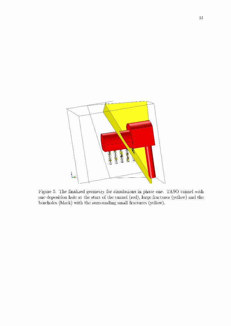
Figure 5: The �nalized geometry for simulations in phase one. TASO tunnel withone deposition hole at the start of the tunnel (red), large fractures (yellow) and theboreholes (black) with the surrounding small fractures (yellow).

32

7 Results

Measurements conducted in the boreholes of Äspö Hard Rock Laboratory were sim-ulated with di�erent models. The stress state of the bedrock was calculated �rst.The �ow simulations can be divided into two phases according to the geometry, asdescribed in the previous section. In the �rst phase of the experiments there were�ve boreholes of 7.6 cm diameter on the �oor of TASO tunnel. Pressure and in-�ow measurements were conducted with focus on borehole 17G01. For the secondphase, holes 17G01 and 18G01 were expanded to 30 cm diameter and additional 14holes were drilled around the previous ones. Again, pressure and in�ow tests wereconducted. All these experiments were simulated using combinations of di�erentmodels for rock and fracture permeabilities.

During in�ow tests, all other holes were sealed, except for the examined one.In the �rst phase, the total in�ow test to the holes succeeded in giving results toonly two holes, i.e., 17G01 and 14G01. In�ow to 17G01 was also measured from adepth range of 0.5�2.97 m, in relation to the tunnel �oor. In phase two, the �owexperiments were conducted on 17G01 and 18G01, and pressure measurements onselected new holes. The in�ow to TASO tunnel �oor was also measured.

For both bedrock and fracture permeability, the computations were done �rstwith constant permeabilites. In addition for bedrock, Volumetric model (Eq. (35)),plain fracture lattice model (Eq. (40)) referred to as Bai, and the compressive frac-ture lattice model (Eq. (42)) referred to as Gangi, were used. The models used forfractures were Bed of Nails (Eq. (22)), Exponential (Eq. (26)), and Angular (Eq.(27)). A summary of the model principles is presented in Table 1, and the usedmodel combination indexing is presented in Table 2.

Table 1: Summary of the used models.

Name Description ReferenceRock modelsVolumetric Isotropic model, volumetric-strain-dependent [17]Gangi Fracture lattice model, fractures follow Bed of Nails [14]Bai Fracture lattice model, rigid rock [15]Fracture modelsBed of Nails Compressing asperity distribution [14]Exponential Derived from a DFN simulation, shear included [4]Angular Empirical model derived based on in situ results [2]

33

Table 2: Indexes of the used fracture and bedrock model combinations.

Fracture | Bedrock Constant Volumetric Gangi BaiConstant 1 5 9 13Bed of Nails 2 6 10 14Exponential 3 7 11 15Angular 4 8 12 16

Table 3: Stress state measured in Äspö.

σ1 σ2 σ3Value (MPa) 30 15 10Angle from North 298 - 208Angle from horizontal plane 0 90 0

7.1 Stress calculation

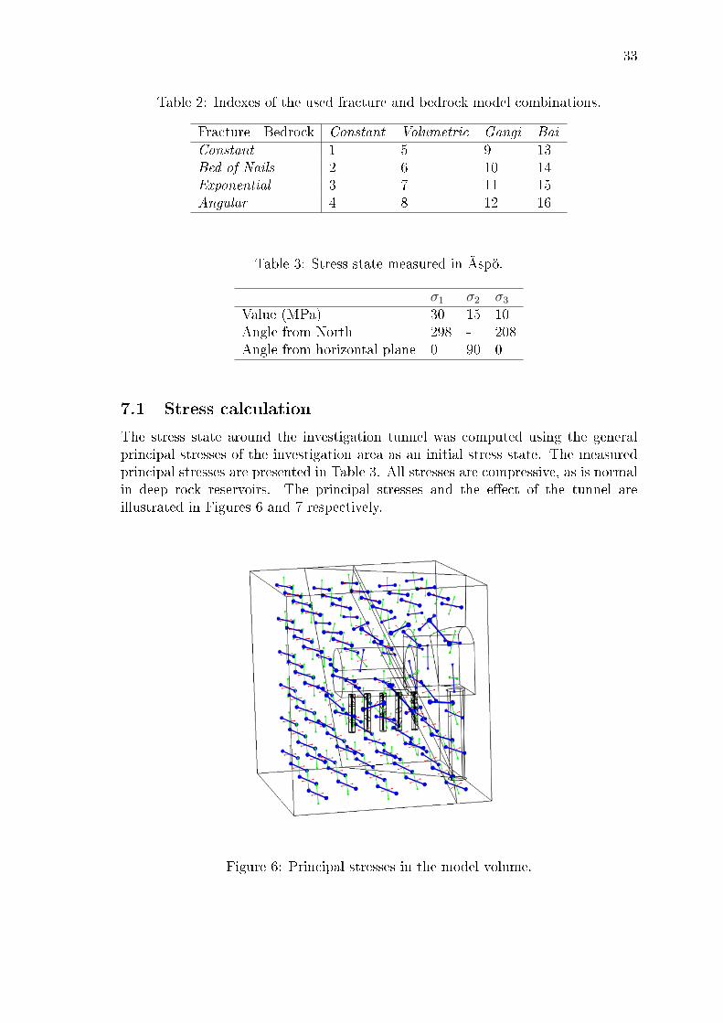
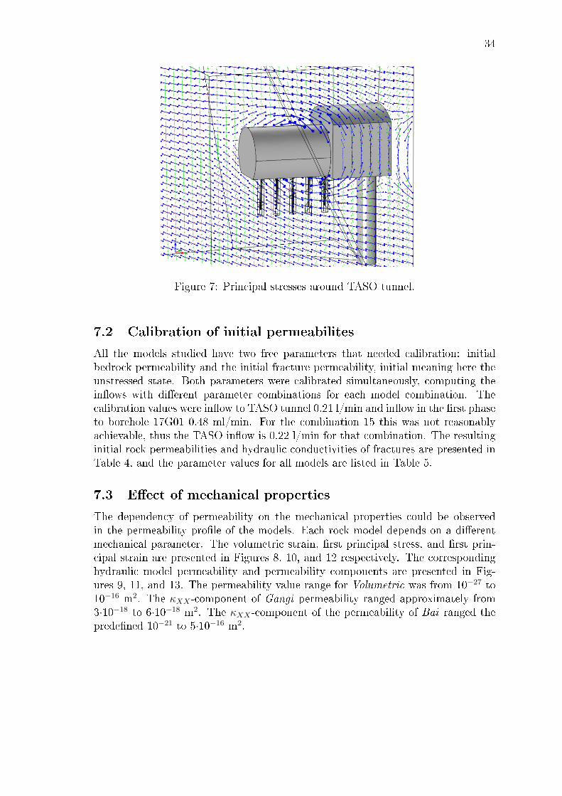
The stress state around the investigation tunnel was computed using the generalprincipal stresses of the investigation area as an initial stress state. The measuredprincipal stresses are presented in Table 3. All stresses are compressive, as is normalin deep rock reservoirs. The principal stresses and the e�ect of the tunnel areillustrated in Figures 6 and 7 respectively.

Figure 6: Principal stresses in the model volume.

34

Figure 7: Principal stresses around TASO tunnel.

7.2 Calibration of initial permeabilites

All the models studied have two free parameters that needed calibration: initialbedrock permeability and the initial fracture permeability, initial meaning here theunstressed state. Both parameters were calibrated simultaneously, computing thein�ows with di�erent parameter combinations for each model combination. Thecalibration values were in�ow to TASO tunnel 0.21 l/min and in�ow in the �rst phaseto borehole 17G01 0.48 ml/min. For the combination 15 this was not reasonablyachievable, thus the TASO in�ow is 0.22 l/min for that combination. The resultinginitial rock permeabilities and hydraulic conductivities of fractures are presented inTable 4, and the parameter values for all models are listed in Table 5.

7.3 E�ect of mechanical properties

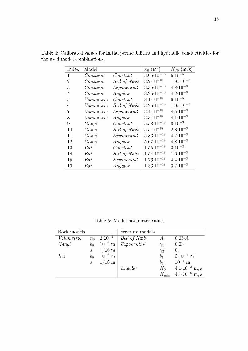
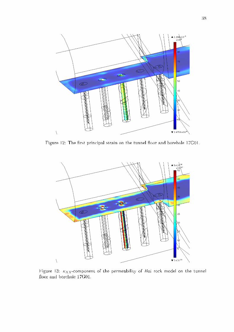
The dependency of permeability on the mechanical properties could be observedin the permeability pro�le of the models. Each rock model depends on a di�erentmechanical parameter. The volumetric strain, �rst principal stress, and �rst prin-cipal strain are presented in Figures 8, 10, and 12 respectively. The correspondinghydraulic model permeability and permeability components are presented in Fig-ures 9, 11, and 13. The permeability value range for Volumetric was from 10−27 to10−16 m2. The κXX-component of Gangi permeability ranged approximately from3·10−18 to 6·10−18 m2. The κXX-component of the permeability of Bai ranged theprede�ned 10−21 to 5·10−16 m2.

35

Table 4: Calibrated values for initial permeabilities and hydraulic conductivities forthe used model combinations.

Index Model κ0 (m2) Kf0 (m/s)1 Constant Constant 3.05·10−18 6·10−52 Constant Bed of Nails 3.2·10−18 1.95·10−33 Constant Exponential 3.35·10−18 4.8·10−34 Constant Angular 3.25·10−18 4.2·10−35 Volumetric Constant 3.1·10−18 6·10−56 Volumetric Bed of Nails 3.25·10−18 1.95·10−37 Volumetric Exponential 3.4·10−18 4.5·10−38 Volumetric Angular 3.3·10−18 4.1·10−39 Gangi Constant 5.58·10−18 3·10−310 Gangi Bed of Nails 5.5·10−18 2.3·10−311 Gangi Exponential 5.83·10−18 4.7·10−312 Gangi Angular 5.67·10−18 4.8·10−313 Bai Constant 1.55·10−18 3·10−214 Bai Bed of Nails 1.54·10−18 1.6·10−315 Bai Exponential 1.76·10−18 4.4·10−316 Bai Angular 1.33·10−18 3.7·10−3

Table 5: Model parameter values.

Rock models Fracture modelsVolumetric n0 3·10−4 Bed of Nails Ar 0.03·AGangi b0 10−6 m Exponential γ1 0.03

s 1/66 m γ2 0.1Bai b0 10−6 m b1 5·10−7 m

s 1/16 m b2 10−4 mAngular K0 4.1·10−3 m/s

Kmin 4.1·10−6 m/s

36

Figure 8: Volumetric strain of the mechanical model on the tunnel �oor and borehole17G01.

Figure 9: Permeability of Volumetric rock model on the tunnel �oor and borehole17G01.

37

Figure 10: The �rst principal stress on the tunnel �oor and borehole 17G01.

Figure 11: κXX-component of the permeability of Gangi rock model on the tunnel�oor and borehole 17G01.

38

Figure 12: The �rst principal strain on the tunnel �oor and borehole 17G01.

Figure 13: κXX-component of the permeability of Bai rock model on the tunnel�oor and borehole 17G01.

39

7.4 In�ow to borehole 17G01

The in�ow to borehole 17G01 has been measured in phase one and with severalmethods in phase two. The measuring-time interval was 400 min, which is longenough to assume the situation to be stationary.

7.4.1 In�ow in phase one

In phase one the measuring-depth interval of borehole 17G01 was 0.5�2.97 m and themeasured in�ow was 0.25 ml/min. The calibration in�ow value was taken from theentire borehole depth. The in�ow from the prescribed depth interval was computedwith the di�erent model combinations; the results are presented in Table 6.

The in�ows computed with di�erent models ranged from 0.21 to 0.30 ml/min,which are close to the measured value. Combinations 1�12 with Constant, Volumet-ric and Gangi gave larger values than Bai, which gave the exact measured valuewith combinations 15 and 16. Among fracture models, in combinations 1�8, Expo-nential gave the smallest in�ow, which was the one closest to the measured value,while Constant and Angular gave the largest in�ows. Combined with Bai rockmodel, Constant and Bed of Nails fracture permeability models gave the smallestvalues. With Gangi rock model, changes between fracture models were too small tobe observed.

Table 6: In�ow to hole 17G01 (ml/min, d = 76 mm), phase one, depth range 0.5�2.97m.

Index Model In�ow1 Constant Constant 0.302 Constant Bed of Nails 0.293 Constant Exponential 0.284 Constant Angular 0.305 Volumetric Constant 0.306 Volumetric Bed of Nails 0.297 Volumetric Exponential 0.288 Volumetric Angular 0.309 Gangi Constant 0.2910 Gangi Bed of Nails 0.2911 Gangi Exponential 0.2912 Gangi Angular 0.2913 Bai Constant 0.2114 Bai Bed of Nails 0.2115 Bai Exponential 0.2516 Bai Angular 0.2517 Measurement 0.25

40

Table 7: In�ow to hole 17G01 (ml/min, d = 300 mm), phase two, depth ranges I:2.1�3.5 m, II: 2.95�3.5 m and III: 3.45�3.5 m.

Index Model I II III1 Constant Constant 0.47 0.27 0.072 Constant Bed of Nails 0.48 0.28 0.093 Constant Exponential 0.50 0.29 0.094 Constant Angular 0.48 0.28 0.095 Volumetric Constant 0.59 0.32 0.076 Volumetric Bed of Nails 0.53 0.28 0.077 Volumetric Exponential 0.55 0.29 0.078 Volumetric Angular 0.54 0.29 0.079 Gangi Constant 0.52 0.29 0.0910 Gangi Bed of Nails 0.50 0.29 0.0911 Gangi Exponential 0.58 0.34 0.1212 Gangi Angular 0.51 0.29 0.0913 Bai Constant 0.03 0.01 0.0014 Bai Bed of Nails 0.03 0.01 0.0015 Bai Exponential 0.04 0.02 0.0116 Bai Angular 0.04 0.01 0.0117 Measurement 0.25 0.20 0.08

7.4.2 In�ow in phase two

The in�ow measurements in phase two for 17G01 were conducted with two di�erentmethods: a nappy test and basic water collection. In a nappy test an absorbing mat,commonly called as a nappy, is placed on the studied area, and later the weight ofthe collected water is measured. The in�ow test was conducted on three depthintervals: 2.1�3.5 m, 2.95�3.5 m and 3.45�3.5 m respectively. The simulation resultsare presented in Table 7. A graphical representation of the in�ows computed for thethree intervals with di�erent model combinations can be found in Figure 14.

The measured relative in�ow increased towards the bottom of the borehole.There were large di�erences between the models, but the simulation results can bedivided into two groups: Bai combinations that gave smaller results, and the othermodels. Combinations 1�12 gave approximately twice as high values for interval Ias what was measured, but close to measured values for interval III. Combinations13�16 gave small values for all areas, though the relative in�ow is greater in regionIII than what was measured. The in�ow distribution along depth di�ered from themeasured results with all combinations, as seen in Figure 14.

In the nappy in�ow test simulation, the borehole was divided into 20-cm-highsections, as were the nappies, distributed over the depth interval 2.25�3.25 m. Nappyindexing goes from top to down. The numeric values for simulated in�ow distribu-tions are shown in Table 8. The in�ow per nappy for each model combination and

41

0 2 4 6 8 10 12 14 16 180

0.1

0.2

0.3

0.4

0.5

0.6

0.7

Model Index

Inflo

w (

ml/m

in)

Figure 14: In�ow to three di�erent sections of borehole 17G01, represented as theheight of each column. The darkest color is for region III (3.45�3.5 m), middle colorfor II, (2.95�3.5 m), and brightest color is for region I (2.1�3.5 m). The red columnpresents the measured results.

the measurements are illustrated in Figure 15.Model combinations 1�12 presented similar behaviour and large in�ow values.

Their in�ow increased slightly with depth, with the exception of nappy 4, wherea slight decrease of in�ow was observed. Of rock models, Volumetric gave largestin�ows, and Constant smallest values. The di�erences between the fracture modelswere relatively small. Constant and Exponential fracture models presented thelargest di�erences.

Bai rock permeability model combinations 13�16 di�ered signi�cantly from theothers. Most importantly the results were small in value. Considering the in�owdistribution, the greatest di�erence was that nappy 5 did not give the largest in�ow,as in other models, but the smallest in�ow. The shape of in�ow along the depthwas now �rst increasing and then decreasing. All four combinations had largest �owinto nappies 2 and 3. Di�erences between the fracture models were negligible.

7.5 In�ow to borehole 18G01

The in�ow to borehole 18G01 was measured only in phase two, for the depth intervalof 2.1�3.1 m. Computed in�ows for di�erent model combinations and the measuredvalues are presented in Table 9.

As with other results, combinations 1�12 exhibited similar behaviour, shown inFigure 16. They all gave large in�ows with little variance between the fracturemodels. The in�ows were close to what was simulated for 17G01 and even largerthan what was measured for 17G01. Bai combinations 13�16 gave again small

42

Table 8: In�ow to hole 17G01 (ml/min, d = 300 mm), nappy test, depth range2.25�3.25 m, nappy indexing runs downwards.

Model | Nappy 1 2 3 4 51 0.05 0.05 0.06 0.05 0.072 0.05 0.05 0.06 0.05 0.073 0.05 0.06 0.06 0.05 0.084 0.05 0.05 0.06 0.05 0.075 0.06 0.07 0.08 0.08 0.096 0.06 0.06 0.07 0.07 0.087 0.06 0.07 0.07 0.07 0.098 0.06 0.07 0.07 0.07 0.089 0.05 0.06 0.06 0.06 0.0810 0.05 0.06 0.06 0.05 0.0811 0.05 0.06 0.06 0.06 0.0912 0.05 0.06 0.06 0.05 0.0813 0.01 0.01 0.01 0.00 0.0014 0.01 0.01 0.01 0.00 0.0015 0.01 0.01 0.01 0.00 0.0016 0.01 0.01 0.01 0.00 0.00Measurement 0 0.023 0.016 0.015 0.024

0 2 4 6 8 10 12 14 16 180

0.01

0.02

0.03

0.04

0.05

0.06

0.07

0.08

0.09

0.1

Model Index

Inflo

w

Figure 15: Nappytest simulations, in�ows to 5 nappies computed with 16 di�erentmodel combinations, index 17 presents the measurement results. Blue = nappy 1,light blue = nappy 2, green = nappy 3, orange = nappy 4, and red = nappy 5.

43

Table 9: In�ow to hole 18G01 (ml/min, d = 300 mm), phase two, depth range2.1�3.1 m.

Index Models 2.1�3.11 Constant Constant 0.402 Constant Bed of Nails 0.403 Constant Exponential 0.424 Constant Angular 0.415 Volumetric Constant 0.526 Volumetric Bed of Nails 0.447 Volumetric Exponential 0.458 Volumetric Angular 0.449 Gangi Constant 0.4310 Gangi Bed of Nails 0.4211 Gangi Exponential 0.4912 Gangi Angular 0.4313 Bai Constant 0.0114 Bai Bed of Nails 0.0115 Bai Exponential 0.0216 Bai Angular 0.0217 Measurement 0.03

0 5 10 15 200

0.1

0.2

0.3

0.4

0.5

0.6

0.7

Model Index

Inflo

w (

ml/m

in)

Figure 16: In�ow to borehole 18G01 at depth range 2.1�3.1 m, computed withdi�erent models (see indexes in Table 9). Measured in�ow to 18G01 in green inindex 17, and measured in�ow to 17G01 in red in index 18 for comparison.

44

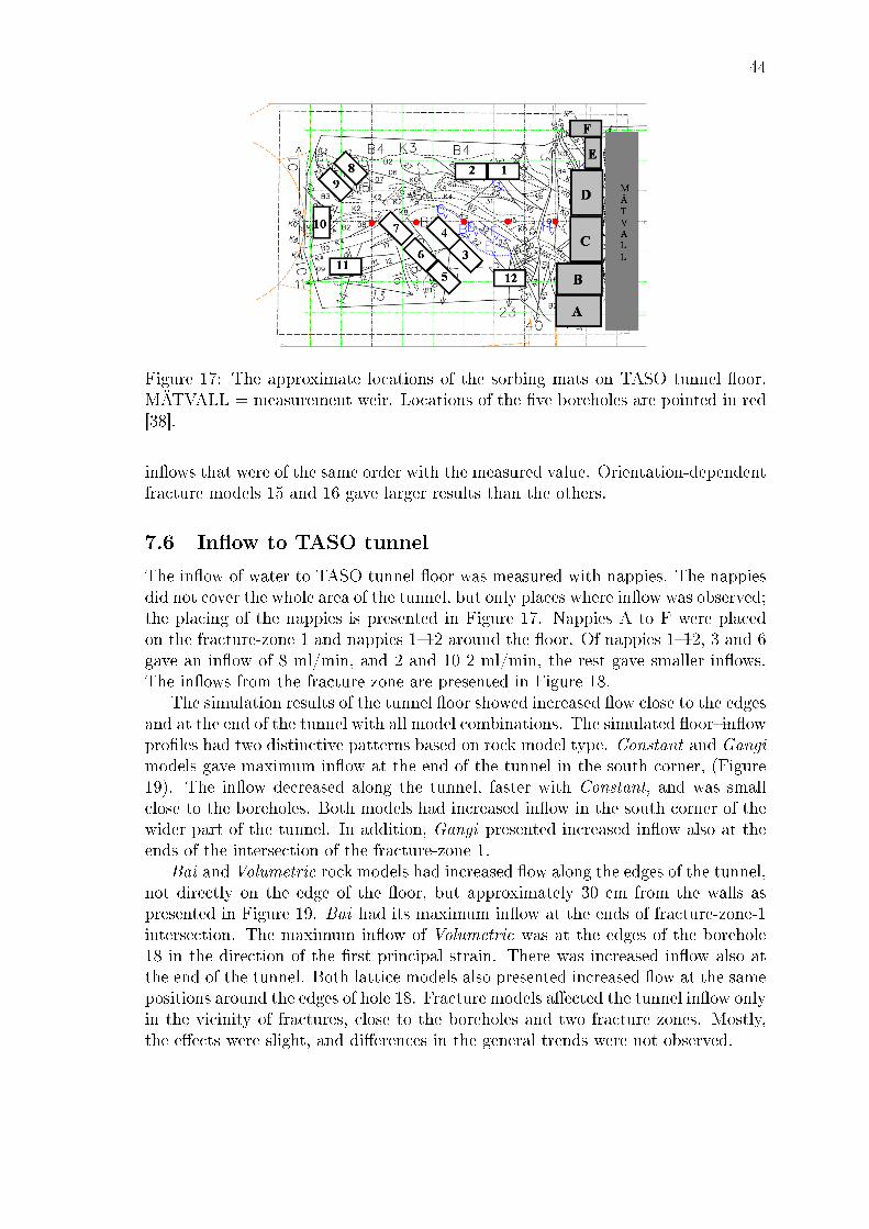
Figure 17: The approximate locations of the sorbing mats on TASO tunnel �oor.MÄTVALL = measurement weir. Locations of the �ve boreholes are pointed in red[38].

in�ows that were of the same order with the measured value. Orientation-dependentfracture models 15 and 16 gave larger results than the others.

7.6 In�ow to TASO tunnel

The in�ow of water to TASO tunnel �oor was measured with nappies. The nappiesdid not cover the whole area of the tunnel, but only places where in�ow was observed;the placing of the nappies is presented in Figure 17. Nappies A to F were placedon the fracture-zone 1 and nappies 1�12 around the �oor. Of nappies 1�12, 3 and 6gave an in�ow of 8 ml/min, and 2 and 10 2 ml/min, the rest gave smaller in�ows.The in�ows from the fracture zone are presented in Figure 18.

The simulation results of the tunnel �oor showed increased �ow close to the edgesand at the end of the tunnel with all model combinations. The simulated �oor�in�owpro�les had two distinctive patterns based on rock model type. Constant and Gangimodels gave maximum in�ow at the end of the tunnel in the south corner, (Figure19). The in�ow decreased along the tunnel, faster with Constant, and was smallclose to the boreholes. Both models had increased in�ow in the south corner of thewider part of the tunnel. In addition, Gangi presented increased in�ow also at theends of the intersection of the fracture-zone 1.

Bai and Volumetric rock models had increased �ow along the edges of the tunnel,not directly on the edge of the �oor, but approximately 30 cm from the walls aspresented in Figure 19. Bai had its maximum in�ow at the ends of fracture-zone-1intersection. The maximum in�ow of Volumetric was at the edges of the borehole18 in the direction of the �rst principal strain. There was increased in�ow also atthe end of the tunnel. Both lattice models also presented increased �ow at the samepositions around the edges of hole 18. Fracture models a�ected the tunnel in�ow onlyin the vicinity of fractures, close to the boreholes and two fracture zones. Mostly,the e�ects were slight, and di�erences in the general trends were not observed.

45

F E D C B A0

20

40

60

80

100

120

140

Nappies

Inflo

w (

ml/m

in)

Figure 18: In�ow values measured from mats F�A.

The in�ow from the fracture zone was controlled in the simulations by the frac-ture permeability model, although the rock permeability model played a role too.All model combinations presented a low peak at the location of mat F, as seen inFigure 20, unlike in the measurements in Figure 18. The outline of the in�ow pro�lefrom the fracture-zone 1 intersection on TASO �oor was quite similar with fracturemodels Constant, Bed of Nails and Angular. They all presented a peak in�ow undermat A and a secondary peak under mat F. The relative size of the peaks dependedon the rock permeability model. Angular gave small in�ow, and Exponential wasthe only fracture model that presented a di�erent pro�le. A sharp peak occurredapproximately at mat B, and the zone of relatively large �ow extended to mat C.A smaller peak was also observed on the other side, approximately between mats Eand F, followed by a signi�cant gap.

7.7 Pressure

The geometry and the permeability distribution determine the pressure contour inthe study domain. Pressure measurements in Äspö were conducted in both phases,one borehole was sealed, sensors within, at the time, while all others were also sealed.

7.7.1 Phase one

The phase one pressure was measured from hole 17G01 from two depth intervals,0.5�2.97 m and 2.0�2.97 m. The value measured for the �rst interval was 0.9�1MPa, and for the latter 1.7 MPa. The modelled pressure distributions were closeto each other, yielding for the �rst interval 0.2�0.9 MPa and at the second interval0.6�1 MPa.

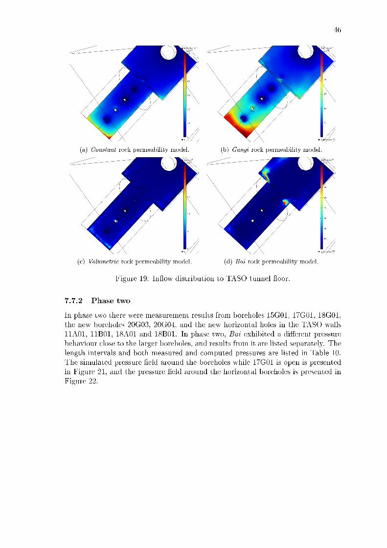
46

(a) Constant rock permeability model. (b) Gangi rock permeability model.

(c) Volumetric rock permeability model. (d) Bai rock permeability model.

Figure 19: In�ow distribution to TASO tunnel �oor.

7.7.2 Phase two

In phase two there were measurement results from boreholes 15G01, 17G01, 18G01,the new boreholes 20G03, 20G04, and the new horizontal holes in the TASO walls11A01, 11B01, 18A01 and 18B01. In phase two, Bai exhibited a di�erent pressurebehaviour close to the larger boreholes, and results from it are listed separately. Thelength intervals and both measured and computed pressures are listed in Table 10.The simulated pressure �eld around the boreholes while 17G01 is open is presentedin Figure 21, and the pressure �eld around the horizontal boreholes is presented inFigure 22.

47

(a) Constant fracture permeability model. (b) Angular fracture permeability model.

(c) Bed of Nails fracture permeability model. (d) Exponential fracture permeability model.

Figure 20: Out�ow distribution pro�le from fracture zone 1 to TASO tunnel, com-puted with di�erent fracture models and Gangi rock model. The layout is similar toFigure 18. Discontinuity in (d) is due to an intersecting line in the geometry. Therelatively large element size is clearly visible in the �gure.

Table 10: Measured and computed pressures for di�erent boreholes in phase 2.

Borehole Section (m) P (MPa) P (MPa) P (MPa)Measured 1�12 13�16

15G01 2.1�3.03 0.5 0.6�0.7 0.4�0.617G01 2.11�2.97 0.5 0.7�0.9 0.1218G01 1.42�3.06 0.4 0.7�1.1 0.1�0.1220G04 2.0�3.5 1.05 1�1.4 0.9�1.320G03 2.0�3.5 0.9 0.9�1.3 0.6�1.211A01 1.01�10 2.7 0.5�1.9 0.5�1.911B01 1.24�10 0.3 0.3�1.1 0.3�1.118A01 1.11�10 2.6 0.6�2.6 0.6�2.618B01 1.28�10 2.1 0.4�1.5 0.4�1.5

48

Figure 21: Pressure �eld around the boreholes, while borehole 17G01 is open.

Figure 22: Pressure �eld around the horizontal boreholes (Pa).

49

8 Discussion

Sixteen combinations of rock and fracture permeability models were used for simula-tions of groundwater �ow in stressed bedrock. Three rock permeability models andthree fracture permeability models were used in addition to constant permeabilitymodels. The model naming and principles are presented in Table 1 and the modelcombination indexing is presented in Table 2. The simulations were conducted intwo phases that have a di�erent geometry; in phase one there were �ve boreholes ofthe same diameter, and in phase two, two of the boreholes were enlarged. All modelswere found to work well for the purpose of the simulation in phase one. In phasetwo, one of the rock permeability models poses numerical problems, but the othermodels give credible results. No single model can replicate the observed behaviour,but each model brings out di�erent aspects of the phenomenon. From the resultsand calibration it is evident that the rock �ow model dominates in a geometry suchas in this work, mostly rock and a couple of fractures here and there.

8.1 Model implementation

The implementation of the model geometry leaves a lot of room for questions anderrors, but when modelling in situ experiments, data is always lacking. Despitethe systematic �ltering procedure, including a few of the reported fractures is quitearbitrary and a lot of information from BIPS and core analysis is lost on the way.However, including observed fractures has more basis in reality than a completelystatistical fracture network. During the elimination process of fractures before build-ing the geometry, when two fractures are too close to each other, one is eliminated.The algorithm chooses the one placed �rst in the list to be eliminated, and no at-tention is paid on the fracture properties. Making this selection by hand would beslow, and a signi�cant improvement in the result would not be guaranteed.

The models of phase two include all the same fractures as in the �rst phase and inaddition the reported two new fractures. On the other hand, it is reported that onlythe two new fractures are identi�ed as �owing structures in the enlarged boreholes.This could be interpreted so that only those two fractures should be included in thegeometry. This choice would change the results especially in hole 18G01, and theupper parts of 17G01, and increase the importance of the rock permeability modeleven more. However, the translation from �rst phase geometry to the second phasewould be even less consistent than at the moment.

The fracture size and shape is another thing that creates large uncertainties.All fractures are assumed planar, because there is no actual information on theirshape. Also the radius chosen for the fractures is somewhat arbitrary. As there isno reported connectivity between the boreholes, it can only be assumed that thefractures do not cross fractures from di�erent boreholes. Another source of con�ictis that the permeability of the rock remains the same, even close to the boreholes,where the fractures are taken into account separately. The overall permeabilityaround the boreholes is thus slightly increased. The importance of the rock perme-ability around the boreholes is increased, which could explain some of the di�erences

50

from the measurements. The calibration results would de�nitely be di�erent, andthe fracture �ow would have a greater e�ect, which is more in line with the mea-surements. The phase two in�ow measurements to 17G01 would have a di�erentdistribution, but the in�ow result of hole 18G01 would not necessarily improve.

8.2 In�ow to borehole 17G01

The in�ow tests to borehole 17G01 in phase one show only little di�erence betweenmodel combinations, which is not surprising as the models are calibrated based onthe total in�ow to this hole. Keeping this in mind, the in�ow values from the lengthinterval along the borehole, presented in Table 6, describe most importantly thedistribution of the in�ow along the hole. The results show that other rock modelsthan Bai rock model tend to slightly overestimate the �ow in the middle part of theborehole. Bai model gives the exact result or a slight underestimate, since it has apronounced maximum �ow point at the bottom of the hole. For the other models,the in�ow from the bottom is smaller, since they have a smoother permeabilitydistribution, hence the larger in�ow to the measurement interval.

In phase two, the in�ow was measured from three di�erent depth intervals of theborehole. As seen in Figure 14, the measured relative in�ow increases towards thebottom of the borehole. For model combinations 1�12 the in�ow values are large,lacking such a relative increase of in�ow with depth, as in the measurements. Whilethere is di�erence in distribution, the in�ow value from interval III is similar to whatwas measured. Rock permeability remains large and saturated close to the tunnelsurface, and no clear change in distribution can be observed.

The bottom part of the borehole is dominated by the e�ect of the fracture addedin phase two, the intersection goes through the bottom of the hole. The reasonfor the systematic di�erence of in�ow distribution from the measurements by allmodels could be in the relative magnitude of rock and fracture permeability. Highrock permeability overestimates �ow in parts where there are no fractures, thuswith lower rock permeability the distribution could be closer to measurements. Therelative magnitude is a result of parameter choices made during the calibration.Another likely reason could be the geometry. The in�ow distribution would bedi�erent if the measured fractures from phase one were not included. If the fractureat the bottom would be the only �owing structure, the amount of �ow would begreater. Also, if the fracture were deeper, and especially, deeper than other fractures,the in�ow distribution would be closer to what was measured.

With Bai model combinations 13�16 the in�ow values are so small in all intervalsthat they are in the limits of the calibration accuracy, and the distribution is evenfurther from what was measured than with the other combinations. This is due tothe small pressure gradient around the enlarged boreholes. The �ow distributiondecreases downwards since the fracture �ow to the bottom of the hole is very strong,and rock �ow from regions close to fractures is diminished.

The general amount of in�ow to the borehole increases due to the new fractureadded in phase two, and the larger area. Another reason for an increase of �owis that the enlarged borehole has larger stresses and strains, which increase the

51

permeabilities. There is no total in�ow value to the borehole reported, and hence itis di�cult to estimate if the measured total in�ow is actually larger in phase two.

8.3 Nappy test

A nappy test was performed on a section of borehole 17G01 in phase two. Nomodel combination can replicate the measured nappy test results, neither in valuenor structure. This is due to the measured zero value for nappy 1, which cannot bereached with models that have a non-zero permeability for rock. Also, the measure-ments report a �owing structure at nappy 2, which can also be seen from the nappy2 in�ow value. As the fracture is not included in the geometry, its e�ect cannot beseen in the simulation results. In the modelled geometry, the only fracture in themeasurement area is at nappy 5.

The nappy test simulation results present the same divided behaviour as seenbefore. Three of the rock models, combinations 1�12, give similar results, where therock model dominates so greatly that the di�erences between the fracture modelscan hardly be seen. The in�ow distribution increases downwards in nappies 1�3,most likely due to the pressure distribution, nappy 4 gives a smaller value andnappy 5 the maximum. The decrease in nappy 4 �ow is due to the fracture in nappy5 that absorbs water from the nappy 4 area. Bai on the other hand gives verysmall results, with a di�erent distribution, as was noticed also in phase two in�owto 17G01. A very small pressure gradient decreases the rock �ow, and strongerfracture �ow dominates. The �ow decreases downwards in the measurement area,and the greatest di�erence to other models is that nappies 4 and 5 give the smallestvalues, instead of the maximum. All combinations have the maximum in�ow atthe bottom of the borehole, but since with Bai rock model the fracture �ow isconsiderably stronger, a larger area around the fracture gets drained.

As can be seen in Figure 15, the rock model controls the distribution of the in�ow,and the fracture model slightly changes the amount of in�ow and the relative sizesbetween in�ows to di�erent nappies. Because there is only one fracture in the nappytest area, the signi�cance of the fracture models is small. The relative di�erence ofin�ow between nappies 2 and 5 covering the observed fractures from the others, isaround the same order in the measurements and combinations 1�12.

The zero in�ow from nappy 1 raises questions of the in�ow sources. The valuemay be a result from measurement inaccuracies, but the reason is probably in therelative magnitudes of rock and fracture �ow. When considering the sources of themodelled �ow, the two observed fractures at nappies 2 and 5 could form the �ow oftheir respective nappies, but the source of the modelled in�ow of nappies 3 and 4is from the rock. However, if nappy 1 value is zero, the observed rock �ow must beconsidered to consist of �ow from fractures too small for observation, which is in linewith the principle of the fracture lattice models. The lack of these fractures wouldexplain the measured zero value. If this is the case, there is no way to predict or evenreplicate the in�ow with Constant or Volumetric models. Although, adding a wellconducting fracture to nappy 2 might decrease somewhat the in�ow from nappy 1.

52

The in�ow from the rock is quite high in the simulations, decreasing it could bringthe results a lot closer to measurements.

8.4 In�ow to borehole 18G01

The computation of in�ow to hole 18G01 brings out a signi�cant di�erence betweenmodel predictions and the measurement. The reported in�ow is very small, alsocompared to the reported in�ow to 17G01. In models 1�12, the permeability ofrock dominates so that even with no fractures in the model, the measured value ofin�ow would be exceeded. In addition, the two fractures at the lower part of theborehole both conduct well according to the fracture models. The second to lowestfracture is optimally oriented for both Exponential and Angular models. Bai modelgives numerically very small values, but as with other combinations, larger valuesthan the in�ow values to hole 17G01. The measured in�ow to 18G01 is only a smallfraction of the in�ow to 17G01.

In the measurements it was reported that at �rst there was no in�ow to hole18G01, and �owing started a while after the boring. This gives a strong indicationthat some sort of deformation might have happened, with the result of increasedtransmissivity. The fracture orientation of the phase two fracture is prone to defor-mation, when examined based on Angular. Exponential gives the fracture a shear tonormal stress ratio kc ≈ 2, which could indicate dilation, depending on the frictionangle of the fracture. The models could be used to �nd fractures that are prone todilation.

8.5 In�ow to TASO tunnel �oor

The simulated in�ow patterns to the TASO tunnel �oor vary between rock models,while fracture models have only small e�ects. The sorbing mats do not cover thewhole �oor, but since they were chosen based on visual inspections of the most�owing areas of the �oor, other areas can be considered to have a smaller in�ow.The sorbing mats can have absorbed water from the ground, falling water from theceiling and the walls, but it is assumed here that all water comes from the �oor.

The most signi�cant in�ow points of the �oor, the points chosen by visual inspec-tion for a mat location, are the fracture intersections. Thus the measurement resultdepends on the fracturing of the TASO �oor. However, no fracture information ofthe �oor was available when building the geometry, and thus in the models in�owto TASO consists of �ow from rock mass. The di�erences between principles mayseem large, but as in the fracture lattice models rock �ow is essentially fracture �ow,these models should be able to replicate the measurements to some extent. The areaaround borehole 18G01 is found to be more conductive, and several mats are placedaround it in the measurements, as is the case at the end of the tunnel. These arefound to match somehow with Constant, Volumetric, and especially Gangi. Bai,however, has an in�ow maximum around nappies E and F, where barely any in�owis registered. Therefore, it can be concluded that Bai is far from what was measured.

53

Mats A to F in Figure 17 are placed on the deformation-zone 1, which is a heavily�owing structure, as in models as well. The heaviest �ow comes from mats A andC, as mats E and F barely register any �ow at all. As the sorbing mat test doesnot separate the �ow out of the fracture zone from the �ow out of the rock, it canonly be assumed that majority of the water comes from the fracture. With thisassumption the in�ow pro�les along fracture zone intersection in Figure 20 can becompared with the measured in�ow in Figure 18. All pro�les are �at when comparedto the measured pro�le, and all have a peak at nappy F. Constant fracture modelpro�le, Figure 20(a) is least similar to the measurements. Exponential is the onlyfracture model taking the shear stress into account, and that can be seen from themore complex in�ow pro�le.

All models have the small peak at mat F since the corner is an in�ow point for alarge area of the fracture. However, this phenomenon is completely lacking from themeasurements. This could indicate that the north side of the tunnel has decreased�ow compared to the south side. This theory is supported also by the horizontalpressure measurements. This is partly due to the other tunnel (Figure 3) that isclose to TASO on the northern side.

8.6 Pressure measurements

The pressure �elds are realistic, follow the measurements to a large extent, and thepressure values give insight to the fracture connectivity. Only Bai has in some casesa signi�cantly di�erent pressure distribution from the others. The high maximumpermeability values of Bai near the expanded boreholes of the phase two geometrycause the pressure in these boreholes to drop to the tunnel boundary pressure,whatever their boundary condition.

In phase one the measured pressure for the �rst interval of 17G01 is of the sameorder than what is computed at the lower level of the interval. More extensiveconnectivity at the topmost part could account for the measured high pressure forthe whole distance. At the lower part of the borehole, the measured pressure is large,2.7 MPa compared to the simulated 0.6�1 MPa. This indicates a good connectivityto much deeper in the bedrock, for example a deep fracture.

In phase two the measured pressure values for the original G01 type boreholesare slightly smaller than those given by combinations 1�12. Bai values are in generalslightly smaller than the others, and in some cases give a slightly better estimate dueto the smaller values. However, for the enlarged boreholes 17G01 and 18G01 Baicombinations give very small pressures, due to the large total permeability aroundthe enlarged boreholes. Between the two phases of the experiment, the measuredpressure in hole 17G01 decreases signi�cantly. The enlargement of the boreholeseems to destroy some connection deeper to the rock.

In the case of the horizontal boreholes, as they are 10 meters long, they coverquite a range of pressures in the model. The measured pressure values are large,except the inner pressure on the B side. 11A01 is clearly well connected to the deeperparts, away from the tunnels, as the measured pressure value is so high, seen in Table10. Both holes at the end of the tunnel give quite large measured values. 11B01

54

on the other hand is placed between tunnels, as seen in Figure 3, hence the smallersimulated values. The di�erences from the simulated pressure �elds would lead toconclude that there are higher pressures around TASO than what the simulationssuggest, with the exception of 11B01 that is well connected with the low pressurearea between tunnels.

Overall the pressure measurements showed that the models are close to what ismeasured, but there are some over- and underestimates. Too large simulated pres-sures are found in the vicinity of the tunnel, and too small can be found particularlyin the long horizontal boreholes. The underestimates could be corrected by chang-ing the pressure boundary condition, but a more probable and less practical causeof error is the lacking fracture and connectivity data. The tendency could indicatethat the permeability is in general larger close to the tunnel and smaller deep in therock.

8.7 Comparison of the models

The model results showed a divided behaviour. Constant, Volumetric and Gangirock models give similar results in shape and magnitude, while Bai combinationsgive markedly di�erent results. Except for this division, di�erences between modelswere small. There is no single model that would outperform the others, but bettermodels can be named, depending on the type of results wanted. It makes a di�erenceif a better value for in�ow, or a more accurate in�ow distribution is wanted, whencomparing the models.

Constant and Gangi are similar to some extent, even though one is isotropic andthe other diagonal, since the change in permeability magnitude in Gangi is less thanan order of magnitude per component. In Bai, on the other hand, the change is �veorders of magnitude per component and the permeability is diagonal. This causeslarge permeability magnitudes, and signi�cant di�erences between directions, whichlead to numerical problems. Volumetric has permeability varying for more than tenorders of magnitude, with no problems during solving, due to its isotropy.

The di�ering results of Bai in phase two are due to its quickly changing perme-ability and a resulting di�erently shaped pressure distribution. Around the expandedboreholes the total permeability is large due to large strains, and this large perme-ability draws down the small pressures of the tunnel �oor. This leads to a smallpressure gradient along the surface of the borehole, and a large gradient right belowthe borehole. The pressure along the borehole evens out, leading to the impressionthat the hole is under an atmospheric pressure boundary condition even if it is not.This only happens with the enlarged boreholes. With Volumetric such very largechanges of permeability magnitude around the hole take place, but there are bothsmall and large total permeabilities around the borehole, and no such change in thepressure distribution occurs.

Constant rock model gives slightly larger results for 17G01 in phase one dueto its relatively even in�ow distribution, and in phase two it gives the smallestresults of combinations 1�12, that are still large compared to measurements. BothVolumetric and Gangi models have signi�cantly larger in�ows around the borehole

55

due to permeability variation. The same case is in 18G01. The values are smallestsince there are no large permeability areas around boreholes, such as the othermodels have. Constant rock model is a good choice if the best numeric values arewanted, but even those in�ows are signi�cantly larger than measurements, and othermodels describe the distribution of the �ow better.

Volumetric rock model gives roughly the largest results in every measurement.With this model also the in�ow distribution to 17G01 is the worst, since the volumet-ric strain is constant along vertical lines, preventing the observed vertical di�erencesfrom forming, which can be seen in Figures 14 and 15. Gangi falls between Con-stant and Volumetric when it comes to in�ow values and pro�les. This follows itsformulation, which can be considered as constant, but is slightly stress dependent.Its permeability around the boreholes is vertically constant, as with the Volumetricmodel. Gangi combination 11 gives the best distribution of �ow into 17G01 in phasetwo.

Bai gives the least correct results in phase two with the small in�ows and oppositedistributions from measurements and other models. Also from the TASO in�owtest, the only actual conclusion that can be made is that Bai results do not �t. Thepermeability causes a very small pressure gradient around the enlarged boreholes.In this model also the relative magnitude of fracture �ow is much larger than mostlyin other combinations. On the other hand, the measured pressures and in�ows aresmaller than what was simulated with other combinations, and in several cases Baigives better results. This could indicate that the pressure distribution of Bai couldhave some resemblance to the measured distribution. Such increased permeabilityaround the boreholes, as with Bai, that changes the pressure distribution, could givethe measured smaller in�ows and smaller pressures. Also, in phase one Bai givesthe best results.

Of the fracture models, Bed of Nails gives the smallest in�ows. This is due tothe mathematical formulation of the model that only allows compression. Angularis close to Bed of Nails in values, the range of permeability is not radical in thismodel either. Constant fracture model in�ow values are large, when combined tothe other rock models than Constant, since Constant fracture model transmits waterequally from all over. Exponential has dilation included and gives larger values dueto this property. The magnitude of �ow is partially due to the choice kc = 1, madein the implementation. The value is what has been measured for single fractures,but simulated values for fracture systems are larger. The in�ow distribution ofExponential from fracture zone 1, Figure 20(c), could be called slightly better thanthe others. It has a distinct peak and, if not for the peak at nappy F, wouldresemble the measured in�ow in Figure 18. Also, combination 11 with Exponentialin the phase two in�ow to 17G01 has a slightly better distribution than the others.

Di�erences between modelled results tend to be small, when comparing the mod-elled and measured results, which indicates that the inequality to the measurementresults is caused mainly by conceptual di�erences.

56

9 Conclusions

The e�ect of stress state on bedrock permeability for groundwater was studied bysimulating an in situ experiment. The dependency of permeability on stress wascomputed with di�erent relations, not by making the conventional assumption thathydraulic and mechanical apertures are equal. The approach was found to work wellfor in situ simulations.

Two permeability models were implemented as such, three of the models weredeveloped further to suit the implementation, and a new empirical model for fracturepermeability was derived from previously reported experimental results. The simula-tion geometry was constructed based on the experimental setup of BRIE. COMSOLwas found to be a su�cient tool for the simulations in the applied geometry, whereinthe number of fractures had been reduced.

Due to the geometry implementation and calibration, the e�ect of rock perme-ability was pronounced. The granular approach of the rock structure did not workwell for the studied rock type, neither as compressive grains in a symmetric lattice(Eq. (36), Eq. (38)), nor as randomly placed incompressive grains (Eq. (35)). Aconstant rock permeability or a fracture lattice model were found to be more suit-able for the studied rock. Two of the fracture models (Exponential and Angular)were found to be able to roughly estimate the tendency of fractures to displace anddilate.

In the future, di�erent model geometry and calibration parameters should betested in order to estimate their e�ect on results. Fracture lattice models should beapplied in line with the fracture models, and di�erent in situ sites could be triedout. Comparison with DFN computations would give insight into the consequencesof the choice of concept. The mechanical model could be improved by includingthe fractures, if sti�ness data were available. With the help of the aforementionedstudy suggestions, a suitable model for permeability for the studied rock type canbe found, and the presented method could be used in in situ modelling tasks.

57

References

[1] L. Qiao, R. Wong, R. Aguilera, and A. Kantzas. Determination of Biot's ef-fective stress parameter for permeability of Nikanassin sandstone. In CanadianInternational Petroleum Conference, 2009.

[2] C.J. Talbot and M. Sirat. Stress control of hydraulic conductivity in fracture-saturated Swedish bedrock. Engineering geology, 61(2):145�153, 2001.

[3] S.F. Rogers. Critical stress-related permeability in fractured rocks. GeologicalSociety, London, Special Publications, 209(1):7�16, 2003.

[4] K. Min, L. Jing, and O. Stephansson. Determining the equivalent permeabilitytensor for fractured rock masses using a stochastic REV approach: methodand application to the �eld data from Sella�eld, UK. Hydrogeology Journal,12(5):497�510, 2004.

[5] C.B. Zhou, R.S. Sharma, Y.F. Chen, and G. Rong. Flow�stress coupled per-meability tensor for fractured rock masses. International journal for numericaland analytical methods in geomechanics, 32(11):1289�1309, 2008.

[6] A. Baghbanan and L. Jing. Stress e�ects on permeability in a fractured rockmass with correlated fracture length and aperture. International Journal ofRock Mechanics and Mining Sciences, 45(8):1320�1334, 2008.

[7] Z. Zhao, L. Jing, I. Neretnieks, and L. Moreno. Numerical modeling of stresse�ects on solute transport in fractured rocks. Computers and Geotechnics,38(2):113�126, 2011.

[8] M.A. Biot. General theory of three-dimensional consolidation. Journal of ap-plied physics, 12(2):155�164, 1941.

[9] W.D. Carrier III. Goodbye, Hazen; Hello, Kozeny-Carman. Journal of Geotech-nical and Geoenvironmental Engineering, 129(11):1054�1056, 2003.

[10] J. Kozeny. Über kapillare Leitung des Wassers im Boden. Sitzungsber. Akad.Wiss. Wien, 136:271�306, 1927.

[11] P.C. Carman. Fluid �ow through granular beds. Transactions-Institution ofChemical Engineeres, 15:150�166, 1937.

[12] I. Fatt and D.H. Davis. Reduction in permeability with overburden pressure.Journal of Petroleum Technology, 4(12), 1952.

[13] J.P. Davies and D.K. Davies. Stress-dependent permeability: characterizationand modeling. SPE Journal, 6(2):224�235, 2001.

[14] A.F. Gangi. Variation of whole and fractured porous rock permeability withcon�ning pressure. International Journal of Rock Mechanics and Mining Sci-ences & Geomechanics Abstracts, 15(5):249�257, 1978.

58

[15] M. Bai and D. Elsworth. Modeling of subsidence and stress-dependent hydraulicconductivity for intact and fractured porous media. Rock mechanics and rockengineering, 27(4):209�234, 1994.

[16] M. Bai, F. Meng, D. Elsworth, M. Zaman, and J.C. Roegiers. Numerical model-ing of stress-dependent permeability. International Journal of Rock Mechanicsand Mining Sciences, 34(3):2�e1, 1997.

[17] J.M. Kim and R.R. Parizek. A mathematical model for the hydraulic propertiesof deforming porous media. Ground Water, 37(4):546�554, 1999.

[18] J. Boussinesq. Memoire sur l'in�uence des frottements dans les mouvementsreguliers des �uides. J. Liouville, 13:377�424, 1868.

[19] C. Louis. A study of groundwater �ow in jointed rock and its in�uence on thestability of rock masses. Imperial College of Science and Technology, 1969.

[20] D.T. Snow. Rock fracture spacings, openings, and porosities. Journal of SoilMechanics & Foundations Div, 1968.

[21] F. Jones Jr. A laboratory study of the e�ects of con�ning pressure on fracture�ow and storage capacity in carbonate rocks. Journal of Petroleum Technology,27(1):21�27, 1975.

[22] P.A. Witherspoon, J.S.Y. Wang, K. Iwai, and J.E. Gale. Validity of cubiclaw for �uid �ow in a deformable rock fracture. Water Resources Research,16(6):1016�1024, 1980.

[23] J.A. Greenwood and J.B.P. Williamson. Contact of nominally �at surfaces. Pro-ceedings of the Royal Society of London. Series A. Mathematical and PhysicalSciences, 295(1442):300�319, 1966.

[24] P.A. Witherspoon and J.E. Gale. Mechanical and hydraulic properties of rocksrelated to induced seismicity. Engineering Geology, 11(1):23�55, 1977.

[25] G. Swan. Determination of sti�ness and other joint properties from roughnessmeasurements. Rock Mechanics and Rock Engineering, 16(1):19�38, 1983.

[26] J.E. Gale. The e�ects of fracture type (induced versus natural) on the stress-fracture closure-fracture permeability relationships. In The 23rd US Symposiumon Rock Mechanics (USRMS), 1982.

[27] I.W. Yeo, M.H. De Freitas, and R.W. Zimmerman. E�ect of shear displacementon the aperture and permeability of a rock fracture. International Journal ofRock Mechanics and Mining Sciences, 35(8):1051�1070, 1998.

[28] S. Gentier, E. Lamontagne, G. Archambault, and J. Riss. Anisotropy of �owin a fracture undergoing shear and its relationship to the direction of shearingand injection pressure. International Journal of Rock Mechanics and MiningSciences, 34(3):94�e1, 1997.

59

[29] H.S. Lee and T.F. Cho. Hydraulic characteristics of rough fractures in linear�ow under normal and shear load. Rock Mechanics and Rock Engineering,35(4):299�318, 2002.

[30] Z. Chen, S.P. Narayan, Z. Yang, and S.S. Rahman. An experimental investiga-tion of hydraulic behaviour of fractures and joints in granitic rock. InternationalJournal of Rock Mechanics and Mining Sciences, 37(7):1061�1071, 2000.

[31] K.B. Min, J. Rutqvist, C.F. Tsang, and L. Jing. Stress-dependent permeabilityof fractured rock masses: a numerical study. International Journal of RockMechanics and Mining Sciences, 41(7):1191�1210, 2004.

[32] B.H.G. Brady and E.T. Brown. Rock mechanics: for underground mining.Springer, 2007.

[33] J. Zhang, W.B. Standi�rd, J-C. Roegiers, and Y. Zhang. Stress-dependent �uid�ow and permeability in fractured media: from lab experiments to engineeringapplications. Rock mechanics and rock engineering, 40(1):3�21, 2007.

[34] Kang Feng and Zhongci Shi. Mathematical theory of elastic structures. SpringerBerlin, 1996.

[35] E. Hakami. Aperture distribution of rock fractures. PhD thesis, Royal Instituteof Technology Stockholm, Sweden, 1995.

[36] T. Koyama, N. Fardin, L. Jing, and O. Stephansson. Numerical simulation ofshear-induced �ow anisotropy and scale-dependent aperture and transmissivityevolution of rock fracture replicas. International Journal of Rock Mechanicsand Mining Sciences, 43(1):89�106, 2006.

[37] COMSOL Multiphysics. www.comsol.com. 1.2.2013.

[38] Å. Fransson and M. Åkesson. Äspö Hard Rock Laboratory, Bentonite RockInteraction Experiment. SKB X-XX-XX, To be published.

Series title and numberVTT Technology 127

Title The effect of stress state on groundwater flow in bedrockSimulations of in situ experiments

Author(s) Karita KajantoAbstract The effect of the stress state on the permeability of bedrock for groundwater was

studied by simulating an in situ experiment. Previous studies show that the de-pendency of permeability on stress can have a significant effect on flow. Severalmodels have been developed, but little has been done in order to develop mod-els suitable for in situ applications, such as the deep underground repositoriesfor spent nuclear fuel. In repositories, stress state evolves during the long timeperiod considered in safety assessment. The effect of the changing flow pattern,due to the evolving stress, has to be estimated for, e.g., radionuclide transportcalculations.

Previous work done in the field was reviewed, existing relations betweenstress and permeability were analysed, and suitable relations were selected forthe modelling cases. Rock mass permeability and discrete fracture permeabilitywere treated separately. One new empirical model for fracture permeability waspresented and three models were further developed to be more suitable for 3-Dimplementation. Simulations followed in situ experiments conducted in ÄspöHard Rock Laboratory. The modelling geometry was constructed based on theexperimental setup and the fracture information from the location. The overallstress state in the area was known and the effect of the measurement tunneland boreholes was computed. The stress state was used to compute thegroundwater flow, and the applicability of the chosen models for in situ modellingwas analysed. COMSOL Multiphysics was used as the tool for the simulations.

The simulation results followed the measurements reasonably well, but differ-ences were found with one model. The results show that differences betweenmost of the models were relatively small if inflow rates were compared, however,differences between flow patterns were found. Stress dependency could partlyexplain observed phenomena and qualitative behaviour. Moreover, some of thefracture models were able to identify fractures prone to deformation.

ISBN, ISSN ISBN 978-951-38-8054-5 (URL: http://www.vtt.fi/publications/index.jsp)ISSN-L 2242-1211ISSN 2242-122X (Online)

Date September 2013Language English, Finnish abstractPages 59 p.Name of the projectCommissioned byKeywords Permeability, stress, in situ, bedrock, groundwaterPublisher VTT Technical Research Centre of Finland

P.O. Box 1000, FI-02044 VTT, Finland, Tel. 020 722 111

Julkaisun sarja ja numeroVTT Technology 127

Nimeke Jännitystilan vaikutus pohjaveden virtaukseenkallioperässäPaikkatutkimustulosten mallinnusta

Tekijä(t) Karita KajantoTiivistelmä Jännitystilan vaikutusta kallioperän permeabiliteettiin vedelle tutkittiin simuloimalla

in situ -tilannetta. Aiemmat tutkimukset ovat osoittaneet, että permeabiliteetinriippuvuus jännitystilasta voi vaikuttaa merkittävästi kallion pohjavesivirtaukseen.Erilaisia malleja aiheesta on kehitetty, mutta in situ -mallinnukseen soveltuvienmallien kehitys on jäänyt vähemmälle. Turvallisuusanalyysin pitkän ajanjaksonaikana jännitystila kalliossa loppusijoitussyvyydellä muuttuu. Muuttuvan jännityk-sen virtaukseen aiheuttamat muutokset tulee ottaa huomioon radionuklidienkulkeutumislaskennassa.

Tässä työssä käytiin läpi alan aiempia tutkimuksia, analysoitiin kehitettyjä jän-nityksen ja permeabiliteetin välisiä malleja sekä valittiin erilaisia tutkittavallekivityypille soveltuvia malleja mallinnustapauksissa käytettäviksi. Kiviaineksenpermeabiliteettia ja yksittäisten rakojen permeabiliteettia käsiteltiin erikseen.Uusi empiirinen rakopermeabiliteettimalli esiteltiin ja aiempia malleja kehitettiinparemmin in situ -mallinnukseen sopiviksi. Simulaatiotapaukset laadittiin ÄspöHard Rock Laboratoryssa tehtyjen mittausten mukaisesti. Laskentageometriavastasi koejärjestelyjä ja alueelta tehtyjä havaintoja. Alueen keskimääräinenjännitystila tunnetaan, ja sen avulla laskettiin mittaustunnelin ja reikien vaikutusmallinnusalueella. Valittujen mallien soveltuvuutta in situ -mallinnukseen analy-soitiin. Laskenta suoritettiin COMSOL Multiphysics -ohjelmistolla.

Mallien tulokset noudattivat mittauksia in situ -mallinnustuloksiksi hyvin, muttajoissain tapauksissa esiintyi selviä eroja. Virtaamatuloksien väliset erot useidenmallien kesken olivat suhteellisen pieniä. Virtausjakaumista löytyi selkeitä eroja,ja jännitystilariippuvuudella voinee selittää joitain tuloksia ja käyttäytymistä. Li-säksi havaittiin, että eräillä rakomalleilla pystyy tunnistamaan raot, joilla on muitasuurempi todennäköisyys deformaatioon.

ISBN, ISSN ISBN 978-951-38-8054-5 (URL: http://www.vtt.fi/publications/index.jsp)ISSN-L 2242-1211ISSN 2242-122X (verkkojulkaisu)

Julkaisuaika Syyskuu 2013Kieli Englanti, suomenkielinen tiivistelmäSivumäärä 59 s.Projektin nimiToimeksiantajatAvainsanat Permeability, stress, in situ, bedrock, groundwaterJulkaisija VTT

PL 1000, 02044 VTT, Puh. 020 722 111

VT

T T

EC

HN

OL

OG

Y 1

27

T

he

effe

ct o

f stress sta

te o

n g

rou

nd

wa

ter fl

ow

in b

ed

roc

k

ISBN 978-951-38-8054-5 (URL: http://www.vtt.fi/publications/index.jsp)ISSN-L 2242-1211ISSN 2242-122X (Online)

The effect of stress state on groundwater flow in bedrock Simulations of in situ experiments

The effect of stress state on groundwater flow in bedrockSimulations of in situ experiments

Karita Kajanto

•VISIONS•S

CIE

NC

E•T

ECHNOLOGY•R

ES

EA

RC

HHIGHLIGHTS

127