the effect of the nonlinearity on gcv applied to conjugate ... · the effect of the nonlinearity on...

Volume 25, N. 1, pp. 111– 128, 2006Copyright © 2006 SBMACISSN 0101-8205www.scielo.br/cam

The effect of the nonlinearity on GCVapplied to Conjugate Gradients in

Computerized Tomography

REGINALDO J. SANTOS1 and Á LVARO R. DE PIERRO2

1Departamento de Matemática, ICEx, Universidade Federal de Minas Gerais

CP 702, 30123-970 Belo Horizonte, MG, Brazil2Department of Applied Mathematics – IMECC, State University of Campinas

CP 6065, 13081-970 Campinas, SP, Brazil

Emails: [email protected] / [email protected]

Abstract. We study the effect of the nonlinear dependence of the iterate xk of Conjugate

Gradients method (CG) from the data b in the GCV procedure to stop the iterations. We compare

two versions of using GCV to stop CG. In one version we compute the GCV function with the

iterate xk depending linearly from the data b and the other one depending nonlinearly. We have

tested the two versions in a large scale problem: positron emission tomography (PET). Our results

suggest the necessity of considering the nonlinearity for the GCV function to obtain a reasonable

stopping criterion.

Mathematical subject classification: 62G05, 92C55, 65F10, 65C05.

Key words: Generalized Cross Validation, Tomography, Conjugate Gradients.

1 Introduction

We consider the problem of estimating a solution x of

Ax + ε = b , (1.1)

where A is a real m × n matrix, b is an m-vector of observations and ε is an

error vector. We assume that the components of ε are random with zero mean,

#647/05. Received: 11/XI/05. Accepted: 30/XI/05.

112 GCV APPLIED TO CONJUGATE GRADIENTS

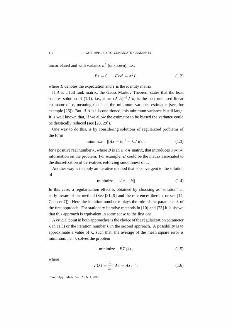
uncorrelated and with variance σ 2 (unknown); i.e.;

Eε = 0 , Eεεt = σ 2 I , (1.2)

where E denotes the expectation and I is the identity matrix.

If A is a full rank matrix, the Gauss-Markov Theorem states that the least

squares solution of (1.1), i.e., x̃ = (At A)−1 At b, is the best unbiased linear

estimator of x , meaning that it is the minimum variance estimator (see, for

example [26]). But, if A is ill-conditioned, this minimum variance is still large.

It is well known that, if we allow the estimator to be biased the variance could

be drastically reduced (see [28, 29]).

One way to do this, is by considering solutions of regularized problems of

the form

minimize ||Ax − b||2 + λxt Bx , (1.3)

for a positive real number λ, where B is an n ×n matrix, that introduces a priori

information on the problem. For example, B could be the matrix associated to

the discretization of derivatives enforcing smoothness of x .

Another way is to apply an iterative method that is convergent to the solution

of

minimize ||Ax − b|| (1.4)

In this case, a regularization effect is obtained by choosing as ‘solution’ an

early iterate of the method (See [31, 9] and the references therein, or see [14,

Chapter 7]). Here the iteration number k plays the role of the parameter λ of

the first approach. For stationary iterative methods in [10] and [23] it is shown

that this approach is equivalent in some sense to the first one.

A crucial point in both approaches is the choice of the regularization parameter

λ in (1.3) or the iteration number k in the second approach. A possibility is to

approximate a value of λ, such that, the average of the mean square error is

minimum, i.e., λ solves the problem

minimize ET (λ) , (1.5)

where

T (λ) = 1

m||Ax − Axλ||2 , (1.6)

Comp. Appl. Math., Vol. 25, N. 1, 2006

REGINALDO J. SANTOS and Á LVARO R. DE PIERRO 113

where xλ is the solution of (1.3) and x is one solution of (1.1). Probably, the

most popular of these methods is Generalized Cross-Validation (GCV) (See

[33, 16]).

If xλ is a estimator for x (the solution of (1.3) or one iterate of a iterative method

convergent to the solution of (1.4)), the influence operator Aλ is defined as

Aλb = Axλ . (1.7)

For the solution of (1.3), the influence operator is given by

Aλb = A(At A + λB)−1 At b (1.8)

If Aλ is given by (1.8), in [6, 13] the GCV function V (λ) was defined as

V (λ) =1m ||b − Axλ||2[1m T r(I − Aλ)

]2 . (1.9)

GCV chooses the regularization parameter by minimizing V (λ). This estimate

is a rotationally invariant version of Allen’s PRESS, or Cross-Validation [1].

In [6, 13] was proven that, if Aλ is given by (1.8), then

|ET (λ) − EV (λ) + σ 2|ET (λ)

<

(2µ1 + µ2

1

µ2

)µ2

1

(1 − µ1)2(1.10)

where µ1 = 1m TrAλ µ2 = 1

m TrA2λ, whenever 0 < µ1 < 1. In [8] Eldén presents

a method to compute the trace-term of the GCV function using bidiagonaliza-

tion. In [12], Golub and Von Matt proposed an iterative method to approximate

the trace-term of the GCV function for large scale problems. In [21], Golub,

Nguyen and Milanfar extended the derivation of the GCV function to under-

determined systems with applications to superresolution reconstruction.

Another approach is to apply an iterative method directly to the least square

problem

minimize ||Ax − b||2

and take as as a ‘solution’ an early iterate of the method. In [10] and [23], it is

proven that this approach is equivalent, in some sense, to (1.3). Now, the role of

the parameter λ is played by the iteration number k and the GCV functional can

be used to choose this number, that is, as a stopping rule, as shown in [32, 25] for



stationary linear iterative methods. It is well known that the Conjugate Gradients

method applied to the normal equations (CGLS) associated to the problem (1.1)

can achieve its best accuracy significantly faster than stationary methods and that

CGLS can be used as a regularizing algorithm (see [22]). However, the iterations

of CG are a nonlinear function of the data vector b, and, as pointed out in [15],

a very good stopping rule should be used. In [15], Hanke and Hansen suggest

a Monte Carlo GCV procedure to stop CGLS and the ν-method ([15], pages

298– 299). But the nonlinearity of the influence operator in the case of CGLS is

not taken into account. While for the ν-method the influence operator is linear

or affine, for CGLS it is nonlinear. However they observe that the application of

their procedure “ can suffer severely from the nonlinearity of CGLS”. Also in [15]

another even more crude approximation is used. In the later case the denominator

of the GCV functional is approximated by the expression(1 − n−p+k

m

)2, where

p is the matrix rank; and this is the same for every value of b ([15], page 307).

The main goal of this paper is to compare a Monte Carlo GCV procedure

deduced in Section 2 that takes into account nonlinearity with another one that

linearizes the influence operator for large scale problems like that arising in

Positron Emission Tomography (PET).

Another alternative to GCV can be the use of the L-curve (see [15]), that is

not considered in this article because of the fact that we wanted to make explicit

the importance of considering the nonlinear part of CG and because of the lack

in that approach (the L-curve) of most of the statistical information provided by

the problem.

In Section 2 we derive an inequality like (1.10), when Aλ is a nonlinear

function of b. We also show how to use a Monte Carlo approach, as in [11],

in order to compute the denominator of our GCV functional. In Section 3 we

describe the implementation of our procedure applied to a preconditioned Con-

jugate Gradients Method (PCCGLS). In Section 4 we present numerical experi-

ments simulating a PET problem and in Section 5 some concluding remarks.



2 GCV for a nonlinear influence operator

We would like to obtain a good estimate for

T (λ) = 1

m||Ax − Axλ||2 , (2.1)

using the relative residual defined by

U (λ) = 1

m||b − Axλ||2 (2.2)

and our information on the error (1.2).

The next result is a technical lemma.

Lemma 1. Let F(λ), g(λ), G(λ), r(λ) and H(λ) be real valued functions with

λ in R and α real number. If

G(λ) = F(λ) + α(1 − 2g(λ)) + r(λ) (2.3)

and

H(λ) = G(λ)

(1 − g(λ))2, (2.4)

then the following expression is valid:

H(λ) − F(λ) − α

F(λ)= 1

(1 − g(λ))2

(−αg(λ)2 + r(λ)

F(λ)+ 2g(λ) − g(λ)2

)(2.5)

Proof. From (2.3) e (2.4) we have that

H(λ) − F(λ) − α

F(λ)

= 1

(1 − g(λ))2

(F(λ) + α(1 − 2g(λ)) + r(λ)

F(λ)− (1 − g(λ))2(F(λ) + α)

F(λ)

)

= 1

(1 − g(λ))2

(1 − α

g(λ)2

F(λ)− (1 − g(λ))2 + r(λ)

F(λ)

),

(2.6)

that implies (2.5). �



Throughout this paper we will assume that the influence operator, defined by

Aλ(b) = Axλ, (2.7)

is a continuously differentiable operator as a function of b, with b varying in an

open set �, that contains Ax , and if we denote by D Aλ(·) the Jacobian of Aλ(·),we have the next result.

Proposition 2. Let {xλ} be a family of estimators for the solution of (1.1), and

(1.2). For each λ, Aλ(·) is continuously differentiable in �, then

EU (λ) = ET (λ) + σ 2

(1 − 2

mT r(D Aλ(Ax))

)+ E(εt Oλ(ε

tε)) , (2.8)

where U (λ) is given by (2.2), T (λ) by (2.1) and the function Oλ(εtε) is such

that ||Oλ(εtε)|| ≤ Mεtε, for some M > 0.

Proof. Expanding the square of the residual of (1.1) and (1.6), at xλ we get that

||b − Axλ||2 − ||Ax − Axλ||2 = ||Ax + ε − Axλ||2 − ||Ax − Axλ||2= ||ε||2 + 2εt(Ax − Axλ) .

(2.9)

Now, expanding Aλ(·) at Ax + ε around the point Ax in Taylor formula:

Aλ(Ax + ε) = Aλ(Ax) + D Aλ(Ax)ε + Oλ(εtε) (2.10)

where Oλ(εtε) satisfies the hypothesis. Using (1.1) and (2.10) above we obtain

Axλ = Aλ(b) = Aλ(Ax + ε) = Aλ(Ax) + D Aλ(Ax)ε + Oλ(εtε) . (2.11)

Dividing (2.9) by m, applying the expectation and using (1.2), (2.11) we obtain

EU (λ) = ET (λ) + 1

mE

(||ε||2

)+ 2

m

[E

(εt Ax

) − E(εt Axλ

)]

= ET (λ) + σ 2 − 2

m

[E

(εt Aλ(Ax)

)

+ E(εt D Aλ(Ax)ε

) + E(εt Oλ(ε

tε))]

= ET (λ) + σ 2[1 − 2

mT r(D Aλ(Ax))

]+ E

(εt Oλ(ε

tε))

,

(2.12�)



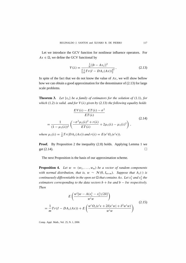
Let we introduce the GCV function for nonlinear influence operators. For

Ax ∈ �, we define the GCV functional by

V (λ) =1m ||b − Axλ||2[

1m T r(I − D Aλ(Ax))

]2 , (2.13)

In spite of the fact that we do not know the value of Ax , we will show bellow

how we can obtain a good approximation for the denominator of (2.13) for large

scale problems.

Theorem 3. Let {xλ} be a family of estimators for the solution of (1.1), for

which (1.2) is valid. and for V (λ) given by (2.13) the following equality holds

EV (λ) − ET (λ) − σ 2

ET (λ)

= 1

(1 − µ1(λ))2

(−σ 2µ1(λ)2 + r(λ)

ET (λ)+ 2µ1(λ) − µ1(λ)2

),

(2.14)

where µ1(λ) = 1m T r(D Aλ(Ax)) and r(λ) = E(εt Oλ(ε

tε)).

Proof. By Proposition 2 the inequality (2.8) holds. Applying Lemma 1 we

get (2.14). �

The next Proposition is the basis of our approximation scheme.

Proposition 4. Let w = (w1, . . . , wm) be a vector of random components

with normal distribution, that is, w ∼ N (0, Im×m). Suppose that Aλ(·) is

continuously differentiable in the open set � that contains Ax. Let xλ1 and xλ

2 the

estimators corresponding to the data vectors b + δw and b − δw respectively.

Then

E

(wt [w − A(xλ

1 − xλ2 )/2δ]

wtw

)

= 1

mT r(I − D Aλ(Ax)) + E

(wt Oλ(ε

tε + 2δ|εtw| + δ2wtw)

wtw

) (2.15)



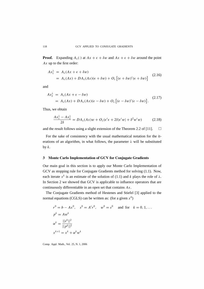
Proof. Expanding Aλ(·) at Ax + ε + δw and Ax + ε + δw around the point

Ax up to the first order:

Axλ1 = Aλ(Ax + ε + δw)

= Aλ(Ax) + D Aλ(Ax)(ε + δw) + Oλ

[(ε + δw)t(ε + δw)

] (2.16)

and

Axλ2 = Aλ(Ax + ε − δw)

= Aλ(Ax) + D Aλ(Ax)(ε − δw) + Oλ

[(ε − δw)t(ε − δw)

].

(2.17)

Thus, we obtain

Axλ1 − Axλ

2

2δ= D Aλ(Ax)w + Oλ(ε

tε + 2δ|εtw| + δ2wtw) (2.18)

and the result follows using a slight extension of the Theorem 2.2 of [11]. �

For the sake of consistency with the usual mathematical notation for the it-

erations of an algorithm, in what follows, the parameter λ will be substituted

by k.

3 Monte Carlo Implementation of GCV for Conjugate Gradients

Our main goal in this section is to apply our Monte Carlo Implementation of

GCV as stopping rule for Conjugate Gradients method for solving (1.1). Now,

each iterate xk is an estimate of the solution of (1.1) and k plays the role of λ.

In Section 2 we showed that GCV is applicable to influence operators that are

continuously differentiable in an open set that contains Ax .

The Conjugate Gradients method of Hestenes and Stiefel [3] applied to the

normal equations (CGLS) can be written as: (for a given x0)

r0 = b − Ax0, s0 = Atr0, w0 = s0 and for k = 0, 1, . . .

pk = Awk

αk = ||sk ||2||pk ||2

xk+1 = xk + αkwk



rk+1 = rk − αk pk

sk+1 = Atrk+1

βk = ||sk+1||2||sk ||2

wk+1 = sk+1 + βkwk

For each k > 0, the operator T (k)(b) = xk is nonlinear and it is continuously

differentiable outside the termination set (closed)

Mk ={

b ∈ Rm |PR(A)b − Ax0 is a linear combination of k eigenvectors of AAt}

,

where PU denotes the orthogonal projection onto the subspace U (i.e., � =(Rn − Mk)). If A is an ill-conditioned operator, then T (k)(·) is discontinuous in

Mk−1, as pointed out by Eicke, Louis and Plato in [7] in the infinite dimensional

context. The same arguments of [7] can be easily used to understand the behavior

of the method in the discrete case. For b in Mk−1, we define bl = b + σl12 ul ,

where ul is the singular vector associated to the singular value σl . From the fact

that bl ∈ Mk it follows that

||T (k)(b) − T (k)(bl)|| = ||A†b − A†bl || = 1

σ12

l

.

Thus, if σl ≈ 0, then ||T (k)(b) − T (k)(bl)|| ≈ ∞. And if b ∈ Mk−1 and bw is b

perturbed by a random vector w, we should also have ||T (k)(b)− T (k)(bw)|| ≈∞. But, usually in ill-posed problems the vector b has all the components of

the singular vectors. It means that b does not belong to a termination set Mk ,

for any k.

Taking into account the results of the preceding section we describe the algo-

rithm for calculating an approximation of the GCV functional (2.13) by using

central differences to approximate the direcional derivative.

Algorithm 1.

(i) Generate a pseudo-random vector w = (w1, . . . , wm)t ∈ Rm from a nor-

mal distribution with standard deviation equal to one, i.e.,

w ∼ N (0, Im×m) .



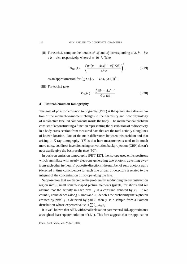
(ii) For each k, compute the iterates xk xk1 and xk

2 corresponding to b, b − δw

e b + δw, respectively, where δ = 10−4. Take

NL(k) =(

wt [w − A(xk1 − xk

2)/2δ]wtw

)2

, (3.19)

as an approximation for(

1m T r [Im − D Ak(Ax)]

)2 ;(iii) For each k take

VNL(k) =1m ||b − Axk ||2

NL(k)(3.20)

4 Positron emission tomography

The goal of positron emission tomography (PET) is the quantitative determina-

tion of the moment-to-moment changes in the chemistry and flow physiology

of radioactive labelled components inside the body. The mathematical problem

consists of reconstructing a function representing the distribution of radioactivity

in a body cross-section from measured data that are the total activity along lines

of known location. One of the main differences between this problem and that

arising in X-ray tomography [17] is that here measurements tend to be much

more noisy, so, direct inversion using convolution backprojection (CBP) doesn’t

necessarily give the best results (see [30]).

In positron emission tomography (PET) [27], the isotope used emits positrons

which annihilate with nearly electrons generating two photons travelling away

from each other in (nearly) opposite directions; the number of such photons pairs

(detected in time coincidence) for each line or pair of detectors is related to the

integral of the concentration of isotope along the line.

Suppose now that we discretize the problem by subdividing the reconstruction

region into n small square-shaped picture elements (pixels, for short) and we

assume that the activity in each pixel j is a constant, denoted by x j . If we

count bi coincidences along m lines and ai j denotes the probability that a photon

emitted by pixel j is detected by pair i , then yi is a sample from a Poisson

distribution whose expected value is∑n

j=1 ai j x j .

It is well known that ART, with small relaxation parameters [18], approximates

a weighted least squares solution of (1.1). This fact suggests that the application



of Conjugate Gradients to the system (4.21) could give similar or better results

[24] and it is a reasonable example to test the capability of GCV as a stopping

rule for CG.

With the objetive of comparing the GCV procedures in Computerized To-

mography we apply the Conjugate Gradients method “ preconditioned” with a

symmetric ART (from algebraic reconstruction technique) method, as presented

recently in [24], i.e. we apply CG to solve the generalized least squares problem

(CGGLS)

min ||C−1ω (b − Ax)||2.

where Cω = (D +ωL)D− 12 , if AAt = L + D + Lt , where L is the strictly lower

triangular part and D the diagonal of AAt respectively.

This corresponds to apply CG to the system

AtC−tω C−1

ω Ax = AtC−tω C−1

ω b , (4.1)

In the ART method, ω is the relaxation parameter. Here it has a different role,

it is the weight of the lower triangular part of A in the preconditioning. When ω

is zero, this corresponds to a diagonal scaling.

The Conjugate Gradients method applied to (4.21) can be written as:

r0 = C−1ω (b − Ax0), s0 = AtC−t

ω r0, w0 = s0 and for k = 0, 1, . . .

pk = C−1ω Awk

αk = ||sk ||2||pk ||2

xk+1 = xk + αkwk

r k+1 = rk − αk pk

sk+1 = AtC−tω rk+1

βk = ||sk+1||2||sk ||2

wk+1 = sk+1 + βkwk

The elements of the matrix L are not explicitly known, but in [2] was shown

an efficient way to compute the products AtC−tω r and C−1

ω Aw.



In our numerical experiments we used the programming system SNARK93,

developed by the Medical Image Processing Group of the University of Penn-

sylvania [5]. The images to be reconstructed (phantom) were obtained from a

computerized atlas based on typical values inside the brain, as in [18]. The data

collection geometry was a divergent one simulating a typical PET data acqui-

sition [5]. We used a discretization with n = 95 × 95 pixels and the divergent

geometry had 300 views, of 101 rays each, a total number of m = 30292 equa-

tions (8 rays were not considered because their lack of intersection with the

image region). The starting point was a uniform image x0 = (a, . . . , a)t , where

a is an approximation of the average density of the phantom given by

a =∑m

i=1 bi∑mi=1

∑nj=1 ai j

. (4.2)

The choice of a uniform non-zero starting point was advocated by L. Kaufman

[20] and it is widely accepted as the best choice for many researchers in PET.

The vector b was taken from a pseudorandom number generator with a Poisson

distribution (see [19]). The total photon count was 2 022 085, 991 179, 514 925

and 238 172 (monotonically increasing noise).

We have performed experiments applying Algorithm 1 with photon counts

2 022 085, 991 179, 514 925 and 238 172 and with six values of ω, between 0.0

and 0.025. For each value ω and each photon count we repeated the experiments

ten times. The ten tests gave very similar results.

We plotted, for one of the tests, in Figure 1 the functions

1001

952||xk − x ||2, 1

30292||Axk − Ax ||2, VMC − 100 and VHH − 100

against the iteration number k, for ω = 0.0 (diagonal scaling) and ω = 0.025.

Here we call VHH the Monte Carlo GCV function, if we suppose that PCCGLS

is a linear function of the data vector b, as proposed by Hanke-Hansen in [15].

As expected, the minimum of our Monte Carlo GCV function VMC(k) coincides

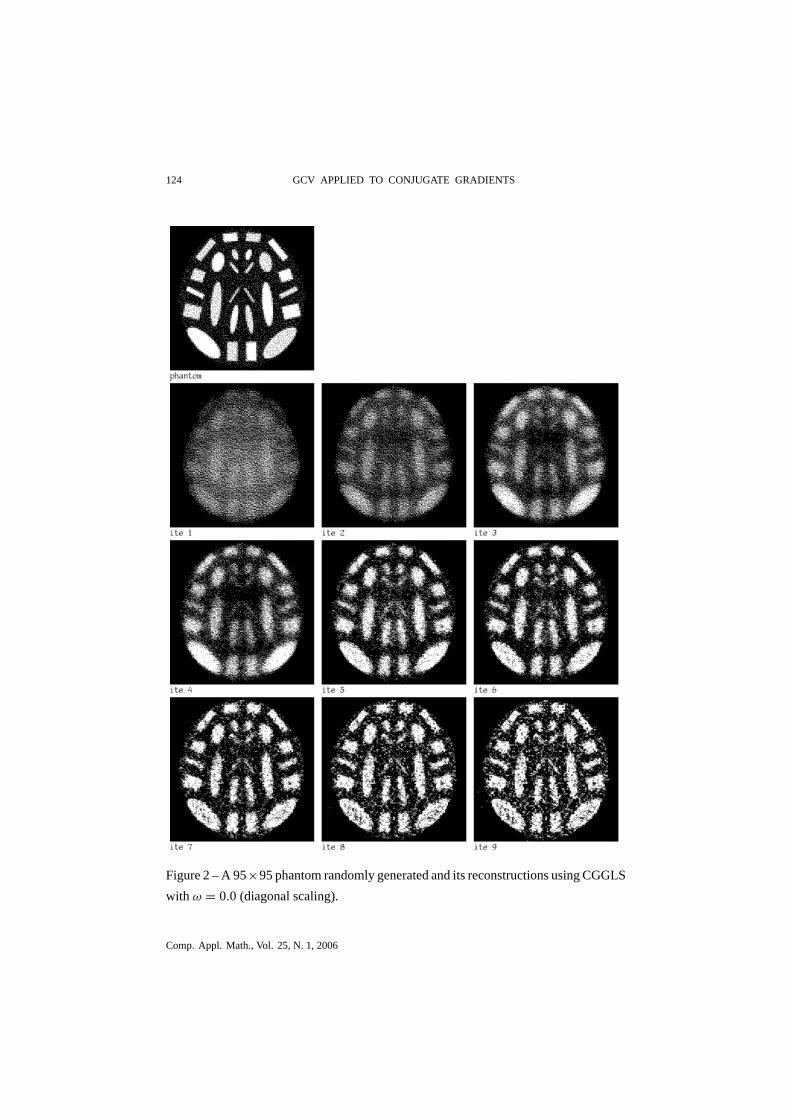
with that of ||A(xk − x)||2, and also the curves are very similar. We can see that

using VHH can give wrong results in the case of Conjugate Gradients. Figures

2 and 3 show the reconstructions corresponding to the curves in row 1 of the

Fig. 1.



0 5 100

50

100

0 5 100

50

100

0 5 100

50

100

0 5 100

50

100

0 5 100

50

100

0 5 100

50

100

0 5 100

50

100

iteration, k0 5 10

0

50

100

iteration, k

Figure 1 – Loss functions for the method CGGLS with ω = 0.0 (diagonal scaling)

(left) and ω = 0.025 (right). The rows 1-4 correspond to 2 022 085, 991 179,

514 925 and 238 172 photon counts, respectively. The solid thin lines correspond

to 100 1952 ||xk − x ||2; the thick ones, to 1

30292 ||Axk − Ax ||2; the dashed lines to transla-

tions of VMC and dotted ones to translations of VHH, i.e., if we suppose that CGGLS is

a linear function of b.



Figure 2 – A 95×95 phantom randomly generated and its reconstructions using CGGLS

with ω = 0.0 (diagonal scaling).



Figure 3 – A 95×95 phantom randomly generated and its reconstructions using CGGLS

with ω = 0.025.



5 Concluding remarks

Iterative methods in Emission Computed Tomography, like RAMLA [4], that

are being used nowadays by PET scanners (see for example http: / / www.

medical.philips.com/us/products/pet/products/cpet/), are fast and produce high

quality pictures (because they take into account the Poisson nature of the noise)

in few iterations. So it was not our goal in this paper to compare Conjugate

Gradient with those methods, but to show that our approximation of GCV is

applicable as a stopping rule to the Conjugate Gradient method for large scale

ill-posed problems, similar to Positron Emission Tomography (very large scale,

not severely ill-posed and relatively large noise in the data). Some authors (see,

for example, [15, 9]) have suggested the use of other approximations to GCV.

Our experimental results show (Fig. 1) that Algorithm 1 gives very good (much

better than Hanke et al’s) approximations for the minimum of ||A(xk − x)||2.

Further research is needed to extend these applications of GCV to more gen-

eral nonlinear methods and nonlinear problems. We also need more specific

asymptotic theoretical results.

Acknowledgements. We are grateful to J. Browne and G.T. Herman for their

support on the use of SNARK93.

Á lvaro R. De Pierro was partially supported by CNPq Grant No. 300969 /

2003-1 and FAPESP Grant No. 2002 / 07153-2, Brazil.

REFERENCES

[1] D.M. Allen, The relationship between variable selection and data augmentation and a method

for prediction. Technometrics, 16(1) (1974), 125– 127.

[2] A. Björck and T. Elfving, Accelerated projection methods for computing pseudoinverse

solutions of systems of linear equations. BIT, 19 (1979), 145– 163.

[3] Åke Björck, Numerical Methods for Least Squares Problems. SIAM, Philadelphia (1996).

[4] J. Browne and A.R. De Pierro, A row-action alternative to the em algorithm for maximizing

likelihoods in emission tomography. IEEE Trans. Med. Imag., 15 (1996), 687– 699.

[5] J.A. Browne, G.T. Herman and D. Odhner, SNARK93 a programming system for image

reconstruction from projections. Technical Report MIPG198, Department of Radiology,

University of Pennsylvania, 1993.



[6] P. Craven and G. Wahba, Smoothing noisy data with spline functions. Numer. Math., 31 (1979),

377– 403.

[7] B. Eicke, A.K. Louis, and R. Plato, The instability of some gradient methods for ill-posed

problems. Numer. Math., 58 (1990), 129– 134.

[8] L. Eldén, A note on the computation of the generalized cross-validation function for ill-

conditioned least squares problems. BIT, 24 (1984), 467– 472.

[9] H. Engl, M. Hanke and A. Neubauer, Regularization of inverse problems. Kluwer Academic

Publishers Group, Dordrecht (1996).

[10] H.E. Fleming, Equivalence of regularization and truncated iteration in the solution of

ill-posed image reconstruction problems. Linear Algebra and its Appl., 130 (1990), 133– 150.

[11] D.A. Girard, A fast ‘Monte-Carlo cross-validation’ procedure for large least squares problems

with noisy data. Numer. Math., 56 (1989), 1– 23.

[12] G. Golub and U. von Matt, Generalized cross-validation for large-scale problems. Journal

of Computational and Graphical Statistics, 6 (1997), 1– 34.

[13] G.H. Golub, M.T. Heath and G. Wahba, Generalized cross-validation as a method for

choosing a good ridge parameter. Technometrics, 21 (1979), 215– 223.

[14] M. Hanke, Conjugate Gradient Type Methods for Ill-Posed Problems. Longman Scientific

& Technical, Essex,UK (1995).

[15] M. Hanke and P.C. Hansen, Regularization methods for large-scale problems. Surv. Math.

Ind., 3 (1993), 253– 315.

[16] P.C. Hansen, Rank-Deficient and Discrete Ill-Posed Problems. SIAM, Philadelphia (1998).

[17] G.T. Herman, Image Reconstruction from Projections: The Fundamentals of Computerized

Tomography. Academic Press, New York (1980).

[18] G.T. Herman and L.B. Meyer, Algebraic reconstruction techniques can be made computa-

tionally efficient. IEEE Trans. Med. Imaging, 12 (1993), 600– 609.

[19] G.T. Herman and D. Odhner, Performance evaluation of an iterative image reconstruc-

tion algorithm for positron emission tomography. IEEE Trans. Med. Imaging, 10 (1991),

336– 346.

[20] L. Kaufman, Implementing and accelerating the EM algorithm for positron emission tomog-

raphy. IEEE Trans. Med. Imag., 6 (1987), 37– 51.

[21] N. Nguyen, P. Milanfar and G. Golub, Efficient generalized cross-validation with applications

to parametric image restoration and resolution enhancement. IEEE Transactions on Image

Processing, 10(9) (2001), 1299– 1308.

[22] R. Plato, Optimal algorithms for linear ill-posed problems yield regularization methods.

Numer. Funct. Anal. Optim., 11 (1990), 111– 118.



[23] R.J. Santos, Equivalence of regularization and truncated iteration for general ill-posed

problems. Linear Algebra and its Appl., 236 (1996), 25– 33.

[24] R.J. Santos, Preconditioning conjugate gradient with symmetric algebraic reconstruction

technique (ART) in computerized tomography. Applied Numerical Mathematics, 47 (2003),

255– 263.

[25] R.J. Santos and A.R. De Pierro, A cheaper way to compute generalized cross-validation as a

stopping rule for linear stationary iterative methods. Journal of Computational and Graphics

Statistics, 12 (2003), 417– 433.

[26] S.D. Silvey, Statistical Inference. Penguin, Harmondsworth (1970).

[27] M.M. Ter-Pogossian et al., Positron emission tomography. Scientific American, October:

170– 181, 1980.

[28] A. van der Sluis and H.A. van der Vorst, Numerical solution of large, sparse linear alge-

braic systems arising from tomographic problems. In G. Nolet, editor, Seismic Tomography.

D. Reidel Pub. Comp., Dordrecht, The Netherlands (1987).

[29] A. van der Sluis and H.A. van der Vorst, SIRT and CG type methods for the iterative solution

of sparse linear least squares problems. Linear Algebra and its Appl., 130 (1990), 257– 303.

[30] Y. Vardi, L.A. Shepp and L. Kaufman, A statistical model for positron emission tomography.

J. Amer. Stat. Assoc., 80(389) (1985), 8– 37.

[31] C. Vogel, Computational methods for inverse problems. SIAM, Philadelphia (2002).

[32] G. Wahba, Three topics in ill-posed problems. In H. Engl and C. Groetsch, editors, Inverse

and Ill-Posed Problems. Academic Press, New York (1987).

[33] G. Wahba, Spline Models for Observational Data. SIAM, Philadelphia (1991).


the effect of the nonlinearity on gcv applied to conjugate ... · the effect of the nonlinearity on...

Documents