the effect of transformer maintenance parameters … for thaiscience/article/61...electric power...

Electric Power Systems Research 72 (2004) 213–224

The effect of transformer maintenance parameterson reliability and cost: a probabilistic model

Panida Jirutitijaroen∗, Chanan Singh

Department of Electrical Engineering, Texas A&M University, College Station, TX 77840, USA

Received 19 February 2004; accepted 30 April 2004Available online 23 July 2004

Abstract

Transformer is an equipment common to most power systems. Preventive maintenance is performed to extend the equipment lifetime.Models relating probability of failure to maintenance activity are proposed in [Panida Jirutitijaroen, Chanan Singh, Oil-immersed transformerinspection and maintenance: probabilistic models, in: Proceedings of the 2003 North American Power Symposium Conference, pp. 204–208].The model parameters which are mean time in each stage, inspection rate of each stage, and probabilities of transition from one stage to others,have an effect on reliability and cost of maintenance. In order to establish a cost-effective maintenance process, analysis of model parametersshould be conducted thoroughly.

This paper develops detailed models relating maintenance parameters to reliability and cost and then investigates the effect of varyingmodel parameters. Simulation results from the proposed model are shown and corroborated by mathematical analysis of a simpler equivalentmodel. The analysis covers mean time to the first failure, maintenance cost, inspection cost, and failure cost.© 2004 Elsevier B.V. All rights reserved.

Keywords: Inspection model; Maintenance; Maintenance model; Probabilistic model; Reliability; Transformer model

1. Introduction

There is relatively little literature on quantifying theeffect of maintenance on reliability in power systems. Aprobabilistic model of the effect of maintenance on relia-bility was first introduced in [2,3]. Based on this generalmodel, oil-immersed transformer inspection and mainte-nance model is proposed in [1] utilizing the concept ofdevice of stage [6].

Model parameters in the proposed model [1] are assumedto be known from data collected. The parameters include in-spection rate of each stage, mean time in each stage, failurecost, maintenance cost, and inspection cost. This paper in-vestigates the effect of model parameters on reliability andmaintenance cost. An equivalent model is introduced forsimpler analysis. The analysis covers mean time to the firstfailure, maintenance and failure cost, and inspection cost.Simulation results of the proposed model are corroboratedby mathematical equations of the equivalent model using

∗ Corresponding author.E-mail address: [email protected] (P. Jirutitijaroen).

first passage time and steady state probability calculations[6].

The objective of this paper is to give an insight into theeffect of the model parameters on reliability and all associ-ated cost.

2. Transformer maintenance model

A general probabilistic model of the effect of maintenanceon reliability is proposed in [2,3]. The model represents thedeterioration process of a device by discrete stages [6]. Thetransformer probabilistic model in [1] utilizes this generalmodel. The model is based on the proposed model in [2,3]and concept of device of stages [6].

In Fig. 1, deterioration process of a transformer is approx-imated by three discrete stages: D1, D2, and D3. At eachstage, oil is inspected to determine its condition. After theinspection, oil condition is determined by the criteria indi-cated in [4,5]. The criteria categorize oil condition into fourgroups ranging from normal (C1) to adverse condition (C4).To simplify the model, C3 and C4 are grouped together.

0378-7796/$ – see front matter © 2004 Elsevier B.V. All rights reserved.doi:10.1016/j.epsr.2004.04.005

214 P. Jirutitijaroen, C. Singh / Electric Power Systems Research 72 (2004) 213–224

Fig. 1. Transformer maintenance model.

These oil conditions are categorized as:

1. Good working condition (C1).2. Required reconditioning before use (C2).3. Poor condition (C3).4. Adverse condition (C4).

Maintenance action is assigned corresponding to the oilcondition. If oil condition is C1, nothing is done. If oil con-dition is C2, C3, or C4, two options are available and areassigned with different probabilities: oil filtering or oil re-placement. For example, if the present stage is D2 with oilcondition C2, the probability of oil filtering will be higherthan oil replacement. On the other hand, if the present stageis D2 with oil condition C3 or C4, the probability of oil re-placement will be higher. After maintenance, the device willhave three options, going to stage D1, D2, or D3. The prob-ability of transferring to other stages depends on the presentstage and maintenance practice.

3. Model parameters

Parameters in transformer maintenance model are listedbelow.

1. Mean time in each stage: These parameters determine thetransition rate of each stage in the deterioration process.

2. Inspection rate of each stage: This parameter can betreated as maintenance rate of each stage under the as-sumption that inspection, test and maintenance actionsare implemented sequentially.

3. Probabilities of transition from one stage to others: Theseparameters are the probabilities of oil condition after theinspection process, probabilities of transferring from anyoil condition to a given stage, probabilities of filteringor replacing the oil, and probabilities of transferring toeach stage after maintenance. These probabilities can betreated as equivalent transition rates from one stage toothers. The equivalent model is introduced to clarify thispoint later.

Notice that model parameters 1 and 3 can be approxi-mated from historical data of oil condition of a physicaltransformer; thus, these parameters are given. However, in-spection rate of each stage can be varied to achieve highreliability with minimum cost. Therefore, this parameter isof the most concern in the analysis.

In the following section, sensitivity analysis of inspectionrate of each stage is implemented on the model in Fig. 1.Other model parameters are listed in Appendix A. The anal-ysis covers two aspects: mean time to the first failure, and allassociated costs (failure, maintenance and inspection costs,respectively). The simulation results from MATLAB are pre-sented and examined in each section.

P. Jirutitijaroen, C. Singh / Electric Power Systems Research 72 (2004) 213–224 215

Fig. 2. The relationship between MTTFF and inspection rates.

4. Sensitivity analysis of inspection rate on mean timeto the first failure (MTTFF)

Mean time to the first failure is the expected operatingtime before failure of the transformer starting from initialstage. This analysis will provide information of how thetransformer operating time changes when the inspection rateof each stage changes.

Let i1 = inspection rate of D1 (per year), i2 = inspectionrate of D2 (per year), i3 = inspection rate of D3 (per year).

The simulation results of the relationship of each inspec-tion rate and MTTFF are shown in Fig. 2a and b.

The following observations can be drawn from these sim-ulation results.

1. In Fig. 2a, MTTFF decreases with i1. This is caused bythe assumption of exponential distribution of time spentin each stage. The exponential distribution implies con-stant failure rate. This is of particular significance in stageD1. This means that the inspections, which lead back toD1, will not improve the time to failure in D1; however,those leading to D2 and D3 will result in degradation.Thus, the effect of inspection will always be degradation.In other words, if we assume an exponential distributionfor stage 1, then maintenance can not be useful.

2. In Fig. 2b, MTTFF increases at a decreasing rate with i2and stays at some value.

3. In Fig. 2c, MTTFF has a positive and linear relationshipwith i3.

Next, the model in Fig. 1 is modified by representingstage D1 by three sub-stages in order to relax the assump-tion of exponential distribution. Although each sub-stage isexponentially distributed, the overall D1 will have a dete-rioration. The simulation results of relationship of each in-spection rate and MTTFF are shown in Fig. 3a–c.

In Fig. 3a, MTTFF increases rapidly when increasing i1and then slightly decreases at high i1. The simulation resultsin Fig. 3b and c give the same observations as in Fig. 2band c.

In conclusion, the simulation results suggest that inspec-tion rate of D1 helps extending MTTFF; however, too highinspection rate of D1 might reduce MTTFF. In addition, in-spection rate of D2 beyond a certain value has a minimalimpact on reliability. Fig. 3c indicates that transformer life-time will be longer with improved inspection rate of D3.

5. Sensitivity analysis of inspection rate on allassociated cost

Costs from maintenance practice in model in Fig. 1 areinspection cost, oil filtering cost, oil replacement cost, andfailure cost. This analysis will provide information about theeffect of inspection rate on all associated cost. We assumecost parameters in Appendix A.

The simulation result of relationship between each inspec-tion rate and all associated costs are shown in Figs. 4–6. The


Fig. 3. The relationship between MTTFF and inspection rate when stage 1 is represented by three sub-stages.

Fig. 4. The relationship between all associated cost and i1.


following observations can be made from the simulationresults.

1. In Figs. 4a, 5a and 6a, failure cost decreases exponentiallyas inspection rate of D1, D2 and D3 increases.

2. In Fig. 4b, maintenance cost first decreases as inspec-tion rate of D1 increases and then increase with inspec-tion rate of D1. The optimal region of inspection rateof D1 that will minimize maintenance cost is 0.5–1 peryear.

3. In Figs. 5b and 6b, maintenance cost increases with in-spection rate of D2 and D3 and stays at constant valueat higher inspection rate of D2 and D3.

4. In Fig. 4c, inspection cost increases linearly with inspec-tion rate of D1.

5. In Figs. 5c and 6c, inspection cost increases as inspectionrate of D2 and D3 increases and remains constant at highinspection rate of D2 and D3.

6. In Fig. 4d, the optimum region of inspection rate of D1that will minimize total cost depends on inspection rate ofD2 and D3. If the inspection rate of D2 and D3 are higher,the optimal value of inspection rate of D1 will be smaller.Failure cost dominates total cost at small inspection rateof D1 while maintenance cost dominates total cost at highinspection rate of D1.

7. In Figs. 5d and 6d, the minimum total cost will occurat very high inspection rate of D2 and D3. Failure costdominates total cost at small inspection rate of D2 andD3 while maintenance cost dominates total cost at highinspection rate of D2 and D3.

In conclusion, simulation result suggests that cost effec-tive maintenance occurs at small inspection rate of D1 andhigh inspection rate of D2 and D3.

The sensitivity analysis of inspection rate on MTTFF andall associated costs are discussed in the previous sectionbased on simulation results of model in Fig. 1. In the nextsection, equivalent mathematical models are presented forsimpler analysis. Equations derived from mathematical anal-ysis will provide an explicit relationship of each inspectionrate with MTTFF and costs.

6. Equivalent models for mathematical analysis

Two equivalent models are introduced to simplify thetransformer maintenance model shown in Fig. 1. The equiv-alent models have three discrete stages representing thedeterioration processes. Assume that maintenance is im-plemented at every inspection, maintenance and inspectionrate of each stage is considered to be an equivalent repairrate.

Let y1 = mean time in stage 1 (year), y2 = mean time instage 2 (year), y3 = mean time in stage 3 (year), µ21 = repairrate from stage 2 to 1 (/year), µ32= repair rate from stage3 to 2 (/year), µ31= repair rate from stage 3 to 1 (/year).

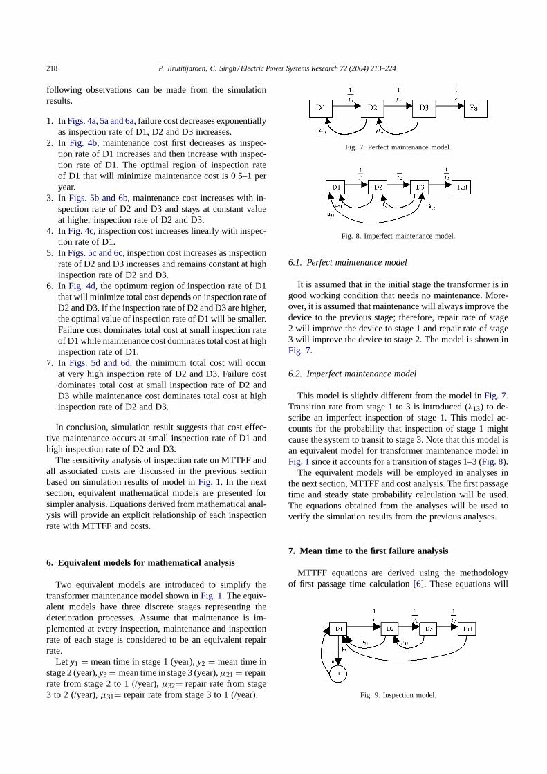
Fig. 7. Perfect maintenance model.

Fig. 8. Imperfect maintenance model.

6.1. Perfect maintenance model

It is assumed that in the initial stage the transformer is ingood working condition that needs no maintenance. More-over, it is assumed that maintenance will always improve thedevice to the previous stage; therefore, repair rate of stage2 will improve the device to stage 1 and repair rate of stage3 will improve the device to stage 2. The model is shown inFig. 7.

6.2. Imperfect maintenance model

This model is slightly different from the model in Fig. 7.Transition rate from stage 1 to 3 is introduced (λ13) to de-scribe an imperfect inspection of stage 1. This model ac-counts for the probability that inspection of stage 1 mightcause the system to transit to stage 3. Note that this model isan equivalent model for transformer maintenance model inFig. 1 since it accounts for a transition of stages 1–3 (Fig. 8).

The equivalent models will be employed in analyses inthe next section, MTTFF and cost analysis. The first passagetime and steady state probability calculation will be used.The equations obtained from the analyses will be used toverify the simulation results from the previous analyses.

7. Mean time to the first failure analysis

MTTFF equations are derived using the methodologyof first passage time calculation [6]. These equations will

Fig. 9. Inspection model.


explain the simulation results in Fig. 3. The analysis is basedon equivalent math models, perfect maintenance model andimperfect maintenance model.


MTTFF is calculated in Appendix B.1.Let T0 = life time without maintenance, TE = extended

life time with maintenance, λ12 = 1/y1 transition rate fromD1 to D2, λ23 = 1/y2 transition rate from D2 to D3, λ3f

= 1/y3 transition rate from D3 to F.Then,

T0 = y1 + y2 + y3 (1)

TE = µ21

λ12λ23+ µ32

λ23λ3f

+ µ21µ32

λ12λ23λ3f

(2)

MTTFF = T0 + TE (3)

The extended time of perfect maintenance model is asummation of all possible combinations of ratios betweenmaintenance rate of the current stage and failure rate of thecurrent and previous stage. Since TE can only be positive inthis model, inspection and maintenance will always extendthe equipment life time.

If the repair rate of each stage is high relative to thetransition rate of that stage and the previous stage (µ21 �λ12λ23, µ32 � λ23λ3f ), the lifetime before failure of thedevice will be high.


MTTFF is calculated in Appendix B.2 using first passagetime technique. Then,

MTTFF = T0 + TE

1 + λ13/λ12 + λ13µ21/λ12λ23(4)

TE = µ21µ31 + µ21µ32 + µ21λ13 + µ32λ13

λ12λ23λ3f

+ µ21

λ12λ23

+ µ31

λ23λ3f

+ µ31

λ12λ3f

+ µ32

λ23λ3f

+ λ13

λ12λ3f

(5)

The relationships of inspection rate of each stage andMTTFF are listed in the following.

7.2.1. Inspection rate of stage 1It is possible that inspection and maintenance will reduce

MTTFF at very high inspection rate of stage 1 (recall thathigh inspection in stage 1 will increase λ13; thus, denomi-nator may be large). This will increase the failure rate fromstage 1 to 3; therefore, MTTFF may decrease. This conclu-sion is verified by the simulation result in Fig. 3a.

7.2.2. Inspection rate of stage 2High inspection rate of stage 2 will increase the repair

rate from stage 2 to 1 (µ21).

Assuming that this repair rate is very high,

MTTFF ≈ 1 + y3(µ31 + µ32 + λ13)

λ13(6)

Then, MTTFF will increase to a constant value. This isverified by the simulation result in Fig. 3b.

7.2.3. Inspection rate of stage 3High inspection rate of D3 will increase the repair rate

from stage 3 to 2 (µ32) and also repair rate of stage 3 to 1(µ31). These rates are linearly related to MTTFF; therefore,the lifetime will increase linearly with inspection rate ofstage 3. This is verified by the simulation result in Fig. 3c.

8. Cost analysis

Cost equations are derived using steady state probabilitycalculation. The cost analyses include failure cost, mainte-nance cost, and total cost. Maintenance cost in this analy-sis includes inspection cost based on the assumption of theequivalent model that maintenance is implemented at everyinspection. These equations will explain the simulation re-sults in Figs. 4–6.


The transitional probability matrix and resulting steadystate probability are derived in Appendix C.1.

Let FC = repair cost after failure (dollar/time), MC= maintenance cost (dollar/time), P(i) = steady state prob-ability of stage i; i=1, 2, or 3, CF = expected annual failurecost (dollar/year), CM = expected annual maintenance cost(dollar/year), CT = expected annual total cost (dollar/year),TR = repair time (year).

8.1.1. Failure cost analysisThe expected failure cost per year is

CF = FC × frequency of failure (7)

CF = FC × P(3) × 1

y3= FC

TR + MTTFF(8)

The failure cost is an average cost over lifetime in onecycle of the device. This indicates that as MTTFF increases,the annual failure cost will reduce and it can also reduce tozero.

Consider the case of very frequent maintenance, this costwill approach zero. On the other hand, without maintenance;this cost will be an average cost over a total life time (lifetime without maintenance plus repair time). This indicatesthat failure cost will be the highest without maintenance;therefore, maintenance helps reducing failure cost.

8.1.2. Maintenance cost analysisThe expected maintenance cost per year is


CM = MC × frequency of maintenance (9)

CM = MC × (P(2)µ21 + P(3)µ32)

= MC(y2µ21 + y3µ32 + y2y3µ21µ32)

TR + MTTFF(10)

Maintenance cost depends on repair rate of stage 2 and3. Without maintenance, this cost will obviously be zero.Consider the case of very frequent maintenance causing thedevice to stay in stage 1 longer, maintenance cost will bethe highest and equal to an average cost over a lifetime instage 1. Therefore, maintenance cost will increase from zeroto some constant value.

8.1.3. Total cost analysisThe expected total cost is a summation of failure and

maintenance cost. Clearly, without maintenance the totalcost will be only a failure cost which is an average cost overa total lifetime. Consider very frequent maintenance, failurecost will be zero while maintenance cost will be the high-est. Thus, total cost is dominated by failure cost at small in-spection rate and is dominated by maintenance cost at highinspection rate.

8.1.3.1. Should we do the maintenance at all? Since main-tenance is introduced in order to reduce the total cost, itshould be implemented only if the highest possible total costwithout maintenance is less than the highest possible totalcost with maintenance, i.e.,

CF(µ21 = 0, µ32 = 0) < CM(µ21 �= 0| µ32 �= 0) (11)

CF(µ21 = 0, µ32 = 0) = FC

TR + T0(12)

CM(µ21 �= 0| µ32 �= 0)

=

CM(µ21 = 0, µ32 → ∞) = MC

y2

CM(µ21 → ∞, µ32 = 0) = MC

y1

CM(µ21 → ∞, µ32 → ∞) = MC

y1

(13)

Thus, the following inequality should be considered.

FC

TR + T0>

MC

y1or

MC

y2(14)

Similarly,

FC

MC>

TR + T0

y1or

TR + T0

y2(15)

The inequality tells that if the ratio of failure cost andmaintenance cost is higher than a constant value, then themaintenance should be implemented. Intuitively, if the fail-ure cost is not expensive, we would rather replace the devicethan maintain it.


The transitional probability matrix and the resultingsteady state probabilities are derived in Appendix C.2.

8.2.1. Failure cost analysisThe expected failure cost per year is

CF = FC × frequency of failure (16)

CF = FC × P(3) × 1

y3= FC

TR + MTTFF(17)

Failure cost equation of this model is the same as thatof perfect maintenance model; however, MTTFF equationis different. From MTTFF analysis, MTTFF will be greaterthan the lifetime without maintenance as long as the proba-bility of transferring from stage 1 to 3 is not high which isusually true. Therefore, failure cost will reduce to a constantvalue as inspection rate of any stage increases. This conclu-sion is verified by simulation results in Figs. 4a, 5a and 6a.

8.2.2. Maintenance cost analysisThe expected maintenance cost per year is

CM = MC × frequency of maintenance (18)

CM = MC × (P(1)λ13 + P(2)µ21 + P(3)(µ31 + µ32))

(19)

If the probability of transferring from stages 1 to 3 is verysmall then the analysis is the same as in perfect maintenancemodel. Maintenance cost will increase from zero to someconstant value when inspection rates of D2 and D3 increase.This is verified by simulation results in Figs. 5b and 6b.However, when inspection rate of D1 increases (probabilityof transferring from stages 1 to 3 is higher), maintenancecost could increase to infinity. This is verified by the simu-lation result in Fig. 4b. It might be the case that the devicecondition gets worse and worse with every inspection andmaintenance.

8.2.3. Total cost analysisFailure cost dominates total cost at small inspection rate

while maintenance cost dominates total cost at high inspec-tion rate. Total cost will be smallest at optimum region ofinspection rate of stage 1 and high inspection rate of stages2 and 3. This conclusion is verified by simulation results inFigs. 4d, 5d and 6d.

Note that in this cost analysis, the inspection cost is ac-counted in the maintenance cost. However, if the inspectionis used only to determine the stage of the device then theinspection cost need to be addressed in the model separately.

9. Inspection model and inspection cost analysis

An inspection stage is added to the perfect mainte-nance model (Fig. 9). Note that the inspection stage has no


transition rate to other stage under an assumption of perfectinspection that the device after inspection will stay in thesame stage. Transitional probability matrix and resultingsteady state probability are derived in Appendix D. TheMTTFF equation is the same as that of the model withoutinspection. Moreover, the steady state probability equationsare the same as those of perfect inspection model.

Intuitively, inspection by itself should not improve oper-ating lifetime of the device since it is introduced only to de-termine the stage of the device. Clearly, the inspection doesnot affect the failure and maintenance cost.

9.1. Inspection cost analysis

Let IC = inspection cost (dollar/time), CI = expected in-spection cost (dollar/year).

The expected annual inspection cost is

CI = IC × P(1) × µI

CI = IC × µI(y1 + y1y2µ21 + y1y2y3µ21µ32)

TR + MTTFF

Inspection cost is a linear function of inspection rate andprobability of being in stage 1; therefore, higher inspectionrate and repair rate of going from any stage to stage 1 willincrease the inspection cost.

9.2. What is the advantage of inspection?

Obviously, inspection increases the total cost. However,inspection is intended to determine the stage of the devicewhich is a crucial issue. Inspection is neither introduced toextend the device lifetime nor to reduce the cost. As long asthe inspection does not cause the system to transit to higherstages, it should be implemented.

10. Conclusion

Analysis of inspection rate of each stage on MTTFF, fail-ure cost, maintenance cost and inspection cost has been rec-ognized in the paper. Simulation results from MATLAB areshown and verified by mathematical equations of the equiv-alent model. The paper suggests the criteria of implement-ing maintenance by comparing the failure and maintenancecost. In addition, inspection model has been constructedfor inspection cost analysis. The analysis suggests theinspection is introduced only to determine the stage ofdevice.

The proposed model in [1] will be selected for differentload type of transformer in the system. The implementationusing Monte Carlo simulation is in progress.

Acknowledgements

The work of this paper was supported by the Power Sys-tem Engineering Research Center.

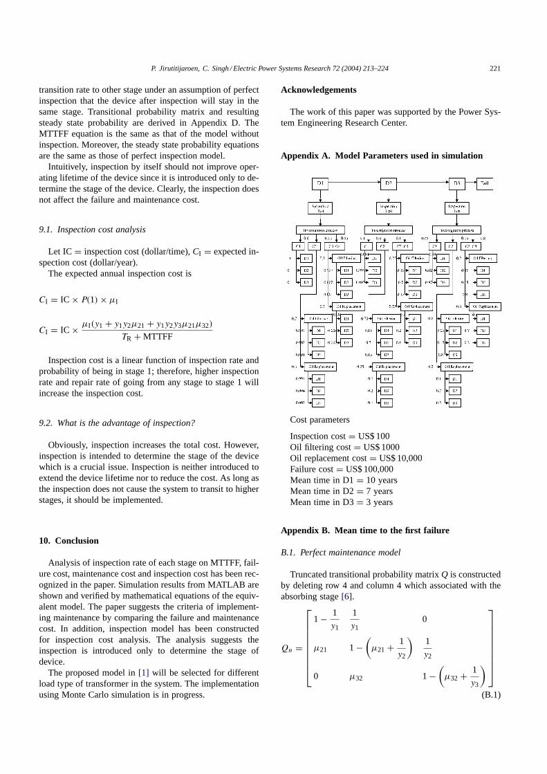
Appendix A. Model Parameters used in simulation

Cost parameters

Inspection cost = US$ 100Oil filtering cost = US$ 1000Oil replacement cost = US$ 10,000Failure cost = US$ 100,000Mean time in D1 = 10 yearsMean time in D2 = 7 yearsMean time in D3 = 3 years

Appendix B. Mean time to the first failure

B.1. Perfect maintenance model

Truncated transitional probability matrix Q is constructedby deleting row 4 and column 4 which associated with theabsorbing stage [6].

Qn =

1 − 1

y1

1

y10

µ21 1 −(

µ21 + 1

y2

)1

y2

0 µ32 1 −(

µ32 + 1

y3

)

(B.1)


The expected number of time intervals matrix is calculatedfrom N = [I − Qn]−1 [6].

det(N) = µ21µ32

y1+ µ21

y1y3+ µ32

y1y2+ 1

y1y2y3

−(

µ32

y1y2+ µ21µ32

y1+ µ21

y1y3

)= 1

y1y2y3(B.2)

Entering from stage 1, MTTFF is the summation of matrixN(1).

MTTFF = y1 + y2 + y3 + µ21y1y2 + µ32y2y3

+ µ21µ32y1y2y3 (B.3)

B.2. Imperfect maintenance model


Qn =

1 −(

λ13 + 1

y1

)1

y1λ13

µ21 1 −(

µ21 + 1

y2

)1

y2

µ31 µ32 1 −(

µ31 + µ32 + 1

y3

)

(B.4)


det(N) = 1

y1y2y3+ λ13

y2y3+ λ13µ21

y3(B.5)

Entering from stage 1, MTTFF is the summation of matrixN(1).

MTTFF = 1

det (N)

(1

y2y3+ 1

y1y3+ 1

y1y2

+ µ21(µ31 + µ32) + µ21

y3+ µ31

y2+ µ32λ13

+ µ31

y1+ µ32

y1+ λ13

y2+ µ21λ13

)(B.6)

Appendix C. Steady state probability

C.1. Perfect maintenance model

Using frequency balance approach, steady state probabil-ity is calculated from

P =

− 1

y1µ21 0 µF

1 1 1 1

01

y2−

(µ32 + 1

y3

)0

0 01

y3−µF

−1

0

1

0

0

(C.1)

Let TR = 1µF

: the repair time (year) then,

det(P) = − µF

y1y2y3(TR + MTTFF). (C.2)

P = 1

(TR + MTTFF)

y1 + y1y2µ21 + y1y2y3µ21µ32

y2 + y2y3µ32

y3

TR

(C.3)

C.2. Imperfect maintenance model


P =

1 1 1 1

1

y1−

(µ21 + 1

y2

)µ32 0

λ131

y2−

(µ31 + µ32 + 1

y3

)0

0 01

y3−µF

−1

1

0

0

0

(C.4)


det(P) = − µF

y1y2y3(TR + MTTFF)

× (1 + y1λ13 + y1y2µ21λ13) (C.5)

Then, the steady state probability is

P = 1

(TR + MTTFF)

y1 + y1y2µ21 + y1y3µ31 + y1y2y3µ21µ31 + y1y2y3µ21µ32

(1 + λ13y1 + λ13µ21y1y2)

y2 + y2y3µ31 + y2y3µ32 + y1y2y3λ13µ32

(1 + λ13y1 + λ13µ21y1y2)y3

TE

(C.6)

Appendix D. Inspection model

D.1. Mean time to the first failure


Qn =

1 −(

µI + 1

y1

)1

y10 µE

µ21 1 −(

µ21 + 1

y2

)1

y20

0 µ32 1 −(

µ32 + 1

y3

)0

1 0 0 0

(D.1)


det(N) = 1

y1y2y3(D.2)

Entering from stage 1, mean time to the first failure is

MTTFF = y1 + y2 + y3 + µ21y1y2 + µ32y2y3

+ µ21µ32y1y2y3 (D.3)

D.2. Steady state probability


P =

1 1 1 1 1

1

y1−

(µ21 + 1

y2

)µ32 0 0

01

y2−

(µ32 + 1

y3

)0 0

0 01

y3−µF 0

µI 0 0 0 −1

−1

1

0

0

0

0

(D.4)

Let TI = Time in inspection stage then,

TI = µI(y1 + µ21y1y2 + µ21µ32y1y2y3) (D.5)

det(P) = µF

y1y2y3(TR + TI + MTTFF) (D.6)

P =

y1 + y1y2µ21 + y1y2y3µ21µ32

TR + TI + MTTFF

y2 + y2y3µ32

TR + TI + MTTFF

y3

TR + TI + MTTFF

TR

TR + TI + MTTFF

µI(y1 + y1y2µ21 + y1y2y3µ21µ32)

TR + TI + MTTFF

(D.7)


The conditional probabilities of stage 1, 2 and 3 giventhat the stages are in working stages (excluding time spentin inspection stage) are

P(1) = y1 + y1y2µ21 + y1y2y3µ21µ32

TR + MTTFF(D.8)

P(2) = y2 + y2y3µ32

TR + MTTFF(D.9)

P(3) = y3

TR + MTTFF(D.10)

These probabilities are the same as in Appendix C.1.

References

[1] Panida Jirutitijaroen, Chanan Singh, Oil-immersed transformer in-spection and maintenance: probabilistic models, in: Proceedings ofthe 2003 North American Power Symposium Conference, pp. 204–208.

[2] J. Endrenyi, G.J. Anders, A.M. Leite da Silva, Probabilistic evaluationof the effect of maintenance on reliability—an application, IEEETrans. Power Sys. 13 (2) (1998) 576–583.

[3] S.H. Sim, J. Endrenyi, Optimal preventive maintenance with repair,IEEE Trans. Reliab. 37 (1) (1998) 92–96.

[4] IEEE Standard, C57.104-1991, IEEE Guide for the Interpretation ofGases Generated in Oil-Immersed Transformers.

[5] IEEE Standard, C57.100-1986, IEEE Standard Test Procedure forThermal Evaluation of Oil-Immersed Distribution Transformers.

[6] C. Singh, R. Billinton, System Reliability Modeling and Evaluation,Hutchinson Educational, London, 1977.

the effect of transformer maintenance parameters … for thaiscience/article/61...electric power...

Documents