The Effect of Vignettingin Hinode/XRT Optical System

Kazunori Ishibashi (NWRA)Rev. 02

(DRAFT)June 12th, 2008

What is vignetting?

[From Wikipedia] Vignetting is a reduction of an image's brightness or saturation at the periphery compared to the image center.

The effect of vignetting in the Hinode/XRT system had not been documented extensively in writing. This led to an incorrect assumption (by yours truly) that the vignetting was negligible. In turn, this led to a (wrong) conclusion that the observed non-uniformity in brightness on the CCD was due to non-uniformly distributed contamination material. But this result was in contradiction to the G-band measurement on the thickness of the contaminants by Bando et al. (J4). Hence, upon request of the J-side XRT team, I have looked at the E2E data taken at XRCF in order to characterize the effect of vignetting for the Hinode/XRT system.

Importance of Vignetting Correction to Science

While depending on the severity of vignetting effect, vignetting-uncorrected images lead to a systemic underestimation in the brightness of an object near the periphery of the CCD (or - more properly - of any FOV).

If the photometric property of data is not important, the effect of vignetting needs not to be compensated. However, the majority of science are (should be) performed with photometrically well-calibrated data and hence one must carefully examine the effect of vignetting to data.

Characterization on the effect of Vignetting

End-To-End (E2E) test data for vignetting

At XRCF/MSFC, X-ray calibration data for vignetting were requested by Sakao et al. and were taken on June 12, 2005 at 30+ different off-axis positions on XRT/CCD detector with Cu-Lα line beam (at E=0.9297keV) as a part of the E2E test.

Focal Point = -798steps (not best), CCD temp = -42.3deg

Exposure Time = 22.6s with [FW1,FW2]=[0,0]

The effect of vignetting was not measured at any other energy during the E2E test. I was unable to find any other suitable data to measure energy dependency in the effect of vignetting.

Data marked as “NG”(logged by Sakao et al.) are omitted.

Analysis Method

Each datum is carefully evaluated for its zero level (dark + bias + readout) and a local background noise around the beam source is measured and subtracted.

The sum of counts in the sampling boxes of 25 x 25 and 200 x 200pix are measured for all the data. The use of two sampling boxes is to determine if the clipping of PSF wing would affect the vignetting measurement significantly.

Also the center of the PSF is estimated by eyes for each datum.

The ratio of photon counts at on-axis ([yaw,pitch]=[0,0]) to that of arbitrary off-axis position provides the effect of reduction in brightness (vignetting) at that arbitrary location on the CCD...(or that is what I thought, but turned out not quite to be the case here... see more later).

Analysis Method (cont.)

CCD X

CC

D

Y

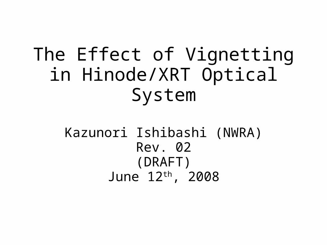
Figure 1

Location of beam positions used for vignetting measurement performed in this analysis. White dots indicate each pointing position.

My understanding is that each E2E image is corrected to CCDX/Y coordinate (the same as theone used nominally in flight).

Analysis Method (cont.)Tabl e 1: Vi gnetti ng Measurement

YYYY_DDD_HH_MM_SS -Yaw -Pi tch Counts X Y (200pi x) (25pi x) (pi xel )

2005_163_14_41_28 4 -16 31422.4 29088.2 1179 2672005_163_14_43_17 16 -14 26701.5 24265.9 1884 3812005_163_14_44_55 10 -14 29446.5 28954.8 1532 3822005_163_14_46_08 4 -14 34093.5 31044.8 1179 3852005_163_14_48_06 -2 -14 35136.5 31007.5 825 3862005_163_14_50_08 -8 -14 32754.2 28912.6 474 3872005_163_14_51_48 10 -8 34352.1 31511.7 1530 7342005_163_14_53_24 4 -8 39014.1 37260.9 1181 7362005_163_14_54_50 -2 -8 39326.3 36793.2 829 7382005_163_14_56_18 18 -2 -1 25382.6 2002 10832005_163_14_57_56 16 -2 29620.7 28128.1 1893 10842005_163_14_59_29 10 -2 35674.7 32355.1 1537 10852005_163_15_01_07 4 -2 42312.2 38686.6 1185 10872005_163_15_02_51 -2 -2 41254.1 38028.3 832 10892005_163_15_05_38 -10 -2 35703.7 33828.3 361 10892005_163_15_07_47 10 4 32283.2 29617.2 1535 14372005_163_15_09_08 4 4 38942 34895.2 1187 14392005_163_15_10_41 -2 4 38251.7 35263.6 833 14412005_163_15_12_25 16 10 24068.2 22805.9 1891 17872005_163_15_13_56 10 10 28290.3 25549.9 1545 17882005_163_15_15_25 4 10 31971.6 29473.8 1189 17902005_163_15_17_07 -2 10 32643.6 30631.3 836 17922005_163_15_18_32 -8 10 29065.3 26857.3 483 17932005_163_15_20_07 4 12 31567.7 28930.7 1189 19092005_163_15_47_47 -13 -3 -1 30148.4 186 10332005_163_15_49_37 -8 -15 28788.2 28036 471 3302005_163_15_55_17 16 -15 27454.4 24962.1 1883 3222005_163_16_03_39 4 -19 -1 27258.1 1177 922005_163_16_08_17 4 -19.5 -1 26921.7 1177 632005_163_16_14_57 4 14 -1 26383 1191 20252005_163_16_33_09 19.5 -3 -1 23273 2097 10232005_163_16_36_10 0 0 42219.7 39391.4 951 1206

(arcmi n)

Table 1Photometric measurement at each Cu-L beam position in order to evaluate the effect of vignetting.

For (my) convenience, the negative valuesof yaw and pitch are listed in the table.

When the beam is placed too close to an edge of the CCD and photometry cannot be done with a larger box, the count is set to -1.

While the offset values [yaw,pitch] are set to be the same, the measured[X,Y] coordinate may vary from time totime. That is not necessarily due to inaccurate measurements by eyes.

Result: First Vignetting Map

Figure 2: First vignetting map (left: linear, right: contour).

Result: First Vignetting Map (cont.)

The scale of reduction due to vignetting varies from 0.49 to 1, although the lower boundary is not well constrained (a result of poor extrapolation).

The effect of vignetting is assumed to be smooth and monotonically declining from the on-axis position.

Not enough data points to constrain the four corners of the CCD.

No data points to evaluate energy dependency.

At least 3% of the uncertainty in the vignetting measurement (mostly due to the background subtraction; not sure about the stability of the beam line at XRCF).

IDL routine min_curve_surf being used to create the map (probably not the best).

Result: First Vignetting Map --> No Good <--

The first vignetting map does not allow the field to be flatten. It seems that the reduction around the periphery of the CCD is estimated to be too much.

Figure 3: Failed attempt to flat-fieldan image with the first vignetting map. The changein color from light green to purple illustrates a steep gradient across the CCD field (Quad I). For unknownreason, the square-root of the first vignettingmap flattens the same imagemore appropriately (see the left panel in the figure).

But for some unknown reason, the square-root of the first vignetting map allowed the images to be flattened more properly. More on that in the following slides.

Square-Rooted Vignetting Map

Figure 4: Square-rooted vignetting map (contour).

The scale of reduction due to vignetting varies from 0.7 to 1. Otherwise the overall structure remains to be the same as the first vignetting map.

The normalized peak resides at coordinate [x0,y0]=[1020,1124].

Square-Rooted Vignetting Map (cont.)

Figure 5: Projected radial profilesof the first (green) and square-rooted(blue) vignetting maps compared withthe theoretical values (red) given by L. Golub (SAO). The radial profileswere derived with [x0,y0]=[1020,1124]as the center.

L. Golub at SAO provides the theoretical values for vignetting based on Goodrich measurement on ground. As shown below, the theoretical radial profile for vignetting closely matches with the square-rooted vignetting map (see Fig 5).

Goodrich Vignetting Map #1

Figure 6: Goodrichvignetting map (contour).

Construct a new vignetting map based on the numbers given by Leon Golub. The on-axis position was chosen to coincide with the same position derived with the E2E data. The profile is assumed to be axially symmetric around the on-axis position. (As I understand it, parts of the mirror entrance are blocked out and hence I'd expect the true map to be not quite concentric like this.)

Goodrich Vignetting Map #2

Figure 7: Goodrichvignetting map (contour).

The same as Goodrich Map #1, except that the vignetting center is placed at the CCD center [1023.5,1023.5].

Vg[angle] = 1.0 - (2/3)x(angle/graze_angle) where

graze_angle = 0.91 degrees

Difference between the Vignetting Maps

Figure 8: Difference between the vignettingmaps (contour). The values are derived as “Sqrt-map - Goodrich map”. The positive differenceis shown in red, negative in blue. The difference is generally below 7%. (Left): Goodrich Map #1; (right): Goodrich Map #2.

Verification of the Vignetting Map

Testing the Vignetting Maps

The three vignetting maps (square-rooted and two Goodrich's) are put to test to see which maps allows X-ray images to be flatten the best.

To do so, I use a set of synoptic images taken nearly at the same time as dither pointing observations (done in October 2007).

Both synoptic and dither-pointing observations observed the same solar disk center region in a short period of time, yet the ROIs of the CCD used to sample the disk center were different (for synoptic, the ROI was roughly [769:1792,769:1792], whereas for dither pointing, the ROI was [1024:2047,1024:2047] for CCD Quadrant I, for instance). Hence if the ratio of these two images were to be taken, the difference in vignetting effect would manifest itself (see the next four slides).

Testing the Vignetting Maps (cont.)

CCD Quadrant I: The radial profile of the flux ratio of images (dither to synoptic) per filter setting. The CCD center ([1024,1024]) is chosen to be the center of the radial distribution. As there is no vignetting correction, the radial profiles show a slope. If each image is corrected for vignetting effect properly, then the flux ratio is expected to be unity at any radius.

Figure 9a

Testing the Vignetting Maps (cont.)

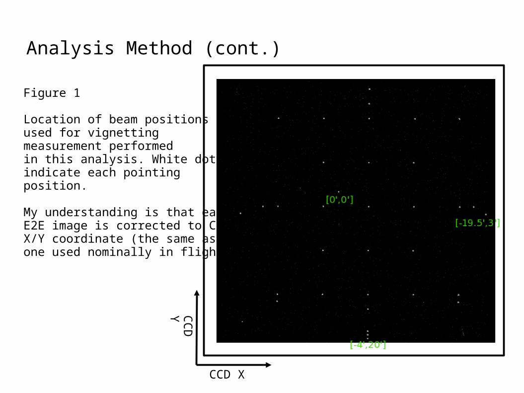
CCD Quadrant II: Ditto as Quadrant I.

Figure 9b

Testing the Vignetting Maps (cont.)

CCD Quadrant III: Ditto as Quadrant I.

Figure 9c

Testing the Vignetting Maps (cont.)

CCD Quadrant IV: Ditto as Quadrant I.

Figure 9d

Testing the Vignetting Maps (cont.)

Now apply vignetting correction using the Sqrt and Goodrich #1 maps (Note: Goodrich #2 map not tested here) , then derive the same radial profile to see if the images are flatter. (In short, the radial profiles are flatter after corrections. Both maps work equally well).

Later on, it is demonstrated that Goodrich #2 Map flattens images better than these two maps tested here.

Testing the Vignetting Maps (cont.)

CCD Quadrant I: The radial profile of the flux ratio of images (dither to synoptic) per filter setting. Black dots show the profile corrected with the Sqrt map. Blue crosses trace the median values of the radial profile (black dots). Red crosses, on the other hand, trace the median value of the radial profile derived with the Goodrich #1 map. It appears that there is very little difference in between them. The radial profile, in any case, is flatter here.

Figure 10a

Testing the Vignetting Maps (cont.)

CCD Quadrant II: Ditto as Quadrant I.

Figure 10b

Testing the Vignetting Maps (cont.)

CCD Quadrant III: Ditto as Quadrant I.

Figure 10c

Testing the Vignetting Maps (cont.)

CCD Quadrant IV: Ditto as Quadrant I.

Figure 10d

Testing the Vignetting Maps (cont.)

Now let us look at the actual image frame (instead of radial profile) to see if there are any local abnormalities produced with vignetting corrections. Ideally, after vignetting correction, each image should look flat (sans some minor changes around active regions or XBPs).

Testing the Vignetting Maps (cont.)

CCD Quadrant I: The flux ratio map per filter setting. On the left of each panel: with Sqrt-map; on the right, with Goodrich #1 map. There seems to be a weak slope across CCD-X direction. Note that Al-mesh images shown on left bottom, Al/poly in top right, and then Ti/poly in right bottom.

Figure 11a

Testing the Vignetting Maps (cont.)

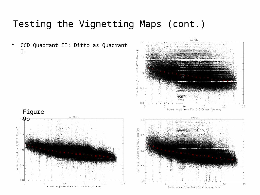
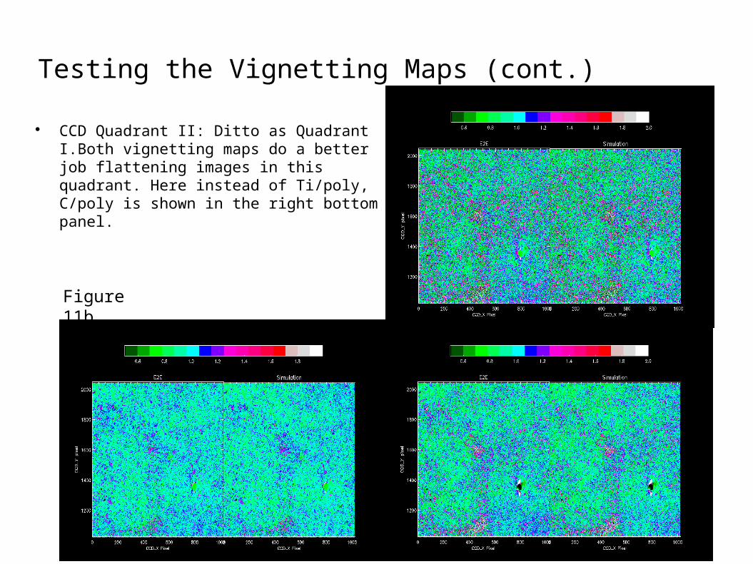
CCD Quadrant II: Ditto as Quadrant I.Both vignetting maps do a better job flattening images in this quadrant. Here instead of Ti/poly, C/poly is shown in the right bottom panel.

Figure 11b

Testing the Vignetting Maps (cont.)

CCD Quadrant III: Ditto as Quadrant I.Both vignetting maps do a better job flattening images in this quadrant. In Al-mesh image, there is a slight pointing offset error.

Figure 11c

Testing the Vignetting Maps (cont.)

CCD Quadrant IV: Ditto as Quadrant I.There seems to be a weak slope toward the right bottom corner of the CCD. So one needs to be cognizant of the artifacts when using the vignetting maps in Quadrants I and IV.

Figure 11d

Testing the Vignetting Maps (cont.)

Both of the vignetting map – Sqrt and Goodrich #1 – appears to work equally well (or poorly, depending on how one looks at the early results).

How about the differences in the quality of “flatness” achieved with Goodrich #2 maps?

Upon comparison, the metric for “flatness” is defined to be how closely the ratio of the vignetting corrected fluxes (shown as a radial profile as before) clusters around unity. For the perfect vignetting, the flatness is perfect and then the ratio becomes unity at any radial angle.

I will repeat the analysis performed to derive Figure 9 in the following.

Testing the Vignetting Maps (cont.)

Al/Mesh Al/Poly

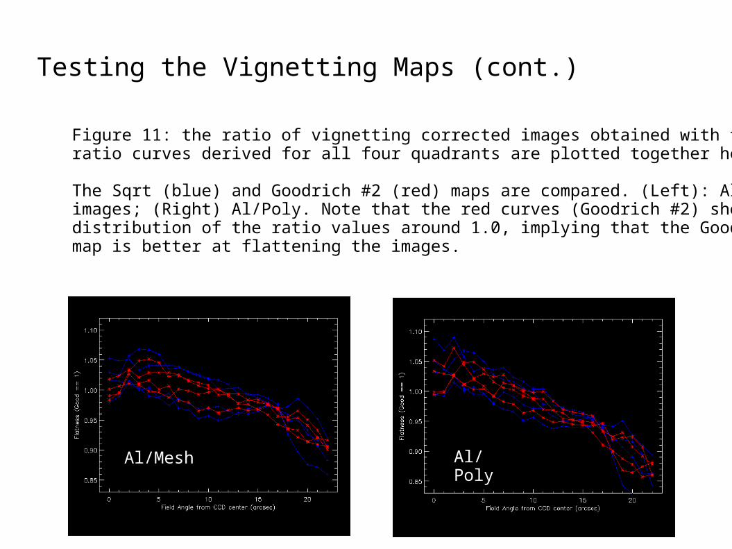
Figure 11: the ratio of vignetting corrected images obtained with two filters. The ratio curves derived for all four quadrants are plotted together here.

The Sqrt (blue) and Goodrich #2 (red) maps are compared. (Left): Al/Meshimages; (Right) Al/Poly. Note that the red curves (Goodrich #2) shows a tighterdistribution of the ratio values around 1.0, implying that the Goodrich #2 (red) map is better at flattening the images.

Testing the Vignetting Maps (cont.)

Al/Mesh Al/Poly

Figure 12: the ratio of vignetting corrected images obtained with two filters.

The Goodrich #1 (blue) and Goodrich #2 (red) maps are compared here. (Left): Al/Mesh images; (Right) Al/Poly. Note that the red curves (Goodrich #2) again shows a tighter distribution of the ratio values around 1.0, implying that the Goodrich #2 map excels in flattening.

Summary on the Testing the Vignetting Maps

The Goodrich #2 map appears to do the best of the three maps. We have a clear winner here (note that it does not mean that the

map is the most optimized vignetting correction map).

The effect of vignetting appears to be weakly dependent of energy (or filter), as the effect of vignetting appears to affect equally the same for all the filter setting (per quadrant...see Figure 9).

Quadrants I and IV (upper and lower right corner of the CCD) show weak slopes, slightly deviating from unity (i.e., the field is not quite flat at these corners).

For the Goodrich map, you can create a map based on the equation: Vg[angle] = 1.0 – (2/3) x (angle/graze_angle)

where graze_angle = 0.91 degrees. Or use nono_vignette.pro by S. Saar (SAO).

Possible culprit for vignetting

A Possible Cause for Vignetting

Off-axis images show a fragmented ring (the three segments of the XRT aperture shown out of focus).This typically implies that some photons were not reflected onto a focal plane by one segment (or a part of) of the XRT mirror due to steep incident angle of the beam. Effectively this would reduce the incident flux by 1/3, or 33%.

Tri-foil pattern

“The Effect of Vignetting” Clarified

The intensity of these three segments changes at various off-axis angle and position. KI considers it due to vignetting.

Gaps due to maskingat the entrance aperture(and not due to vignetting..the effect of these must be incorporated as reduction of the effective area, instead)

Adding a few final words...(not like you haven't heard enough already)

Concluding remarks

When performing filter-ratio analysis on images sampled at the same ROI on the CCD, it appears that there is little need to correct for vignetting. This is true if the vignetting effect is weakly dependent on energy.

Even if one works with 512x512FOV data, at least 5% of systematic underestimation in flux is introduced at the periphery of the FOV.

Shouldn't there be more formal numbers for the true vignetting effect? Like the numbers based on the actual flight mirror model?

It is not understood why the square-rooted vignetting map, based on the E2E data, appears to work fine. Recommend to use Goodrich #2 Map for vignetting correction in any case.

D O N E