Research, Development, and TechnologyTurner-Fairbank Highway Research Center6300 Georgetown PikeMcLean, VA 22101-2296

The Effective Integration of Analysis,Modeling, and Simulation Tools

PublIcATIon no. FHWA-HRT-13-036 AuGuST 2013

FOREWORD

Simulation models used in transportation analysis are not well integrated among different domains (e.g., operations, safety, and environment) and for different levels of analysis (i.e., macro, meso, and micro). This project developed a prototype data hub and data schema using the Network EXplorer for Traffic Analysis (NeXTA) open-source software tool to save users time to input data and to model and display results in a common format. Researchers tested the newly developed model integration approach to address real-world transportation planning, operations, and management problems and demonstrated the approach to transportation planners at Portland Metro and Pima Association of Governments. The test applications validated the open-source data hub functionality by taking existing regional travel demand models from the respective regions, exporting the data to a dynamic traffic assignment model for mesoscopic analysis, exporting to a signal timing optimization tool, and then exporting to a microscopic simulation tool for detailed operations analysis. Preliminary results showed that the data hub prototype overcame many shortcomings associated with integrated modeling applications. The analyses took only 7 to 11 h to complete with the data hub in comparison to 35 to 52 h without the data hub, which is a total time savings of 80 percent. This report documents the findings and recommendations from the research, and it is aimed at model users, managers at modeling agencies, software developers, and researchers who are interested in advancing integrated modeling practices.

Joseph I. Peters Director, Office of Operations Research and Development

Notice This document is disseminated under the sponsorship of the U.S. Department of Transportation in the interest of information exchange. The U.S. Government assumes no liability for the use of the information contained in this document. This report does not constitute a standard, specification, or regulation.

The U.S. Government does not endorse products or manufacturers. Trademarks or manufacturers’ names appear in this report only because they are considered essential to the objective of the document.

Quality Assurance Statement The Federal Highway Administration (FHWA) provides high-quality information to serve Government, industry, and the public in a manner that promotes public understanding. Standards and policies are used to ensure and maximize the quality, objectivity, utility, and integrity of its information. FHWA periodically reviews quality issues and adjusts its programs and processes to ensure continuous quality improvement.

TECHNICAL REPORT DOCUMENTATION PAGE 1. Report No. FHWA-HRT-13-036

2. Government Accession No.

3. Recipient’s Catalog No.

4. Title and Subtitle The Effective Integration of Analysis, Modeling, and Simulation Tools

5. Report Date August 2013 6. Performing Organization Code

7. Author(s) Brandon L. Nevers, Khang M. Nguyen, Shaun M. Quayle, Xuesong Zhou, Ph.D., and Jeffrey Taylor

8. Performing Organization Report No.

9. Performing Organization Name and Address Science Applications International Corporation 8301 Greensboro Drive, Mailstop E-12-3 McLean, VA 22102-2296

10. Work Unit No. (TRAIS) 11. Contract or Grant No.

12. Sponsoring Agency Name and Address Office of Operations Research and Development Federal Highway Administration 6300 Georgetown Pike McLean, VA 22101-2296

13. Type of Report and Period Covered

14. Sponsoring Agency Code

15. Supplementary Notes The Contracting Officer’s Technical Representative (COTR) was Joe Bared, HRDO-20. 16. Abstract The need for model integration arises from the recognition that both transportation decisionmaking and the tools supporting it continue to increase in complexity. Many strategies that agencies evaluate require using tools that are sensitive to supply and demand at local and regional levels. This in turn requires the use and integration of analysis tools across multiple resolutions. Despite this need, many integrated modeling practices remain ad hoc and inefficient.

A concept for an open-source data hub was developed to better enable the exchange of model information across multiple resolutions. All modeling and field data are fed and stored using a unified data schema. Tools within the data hub aid users in modifying modeling network, control, and demand data to match an objective, such as calibrating to field data. Visualization tools were built into the data hub’s core visualization program, NeXTA, along with powerful links to common Web-based tools such as Google Earth®, Google Maps®, and Google Fusion Tables®. The data hub reduces barriers to interfacing models across multiple resolutions and software platforms, which ultimately saves time and reduces costs. 17. Key Words Integrated modeling, Travel demand forecasting, Dynamic traffic assignment, Microsimulation, Data hub, Data schema, Analysis, Modeling, Simulation

18. Distribution Statement No restrictions. This document is available to the public through the National Technical Information Service, Springfield, VA 22161.

19. Security Classif. (of this report) Unclassified

20. Security Classif. (of this page) Unclassified

21. No. of Pages 127

22. Price N/A

Form DOT F 1700.7 (8-72) Reproduction of completed page authorized

ii

SI* (MODERN METRIC) CONVERSION FACTORS APPROXIMATE CONVERSIONS TO SI UNITS

Symbol When You Know Multiply By To Find Symbol LENGTH

in inches 25.4 millimeters mm ft feet 0.305 meters m yd yards 0.914 meters m mi miles 1.61 kilometers km

AREA in2 square inches 645.2 square millimeters mm2

ft2 square feet 0.093 square meters m2

yd2 square yard 0.836 square meters m2

ac acres 0.405 hectares ha mi2 square miles 2.59 square kilometers km2

VOLUME fl oz fluid ounces 29.57 milliliters mL gal gallons 3.785 liters L ft3 cubic feet 0.028 cubic meters m3

yd3 cubic yards 0.765 cubic meters m3

NOTE: volumes greater than 1000 L shall be shown in m3

MASS oz ounces 28.35 grams glb pounds 0.454 kilograms kgT short tons (2000 lb) 0.907 megagrams (or "metric ton") Mg (or "t")

TEMPERATURE (exact degrees) oF Fahrenheit 5 (F-32)/9 Celsius oC

or (F-32)/1.8 ILLUMINATION

fc foot-candles 10.76 lux lx fl foot-Lamberts 3.426 candela/m2 cd/m2

FORCE and PRESSURE or STRESS lbf poundforce 4.45 newtons N lbf/in2 poundforce per square inch 6.89 kilopascals kPa

APPROXIMATE CONVERSIONS FROM SI UNITS Symbol When You Know Multiply By To Find Symbol

LENGTHmm millimeters 0.039 inches in m meters 3.28 feet ft m meters 1.09 yards yd km kilometers 0.621 miles mi

AREA mm2 square millimeters 0.0016 square inches in2

m2 square meters 10.764 square feet ft2

m2 square meters 1.195 square yards yd2

ha hectares 2.47 acres ac km2 square kilometers 0.386 square miles mi2

VOLUME mL milliliters 0.034 fluid ounces fl oz L liters 0.264 gallons gal m3 cubic meters 35.314 cubic feet ft3

m3 cubic meters 1.307 cubic yards yd3

MASS g grams 0.035 ounces ozkg kilograms 2.202 pounds lbMg (or "t") megagrams (or "metric ton") 1.103 short tons (2000 lb) T

TEMPERATURE (exact degrees) oC Celsius 1.8C+32 Fahrenheit oF

ILLUMINATION lx lux 0.0929 foot-candles fc cd/m2 candela/m2 0.2919 foot-Lamberts fl

FORCE and PRESSURE or STRESS N newtons 0.225 poundforce lbf kPa kilopascals 0.145 poundforce per square inch lbf/in2

*SI is the symbol for th International System of Units. Appropriate rounding should be made to comply with Section 4 of ASTM E380. e(Revised March 2003)

iii

TABLE OF CONTENTS

EXECUTIVE SUMMARY ...........................................................................................................1

INTRODUCTION..........................................................................................................................5 CHARACTERISTICS OF EFFECTIVE INTEGRATION ................................................6 MARKET DEMAND FOR INTEGRATION TOOLS ........................................................7

MULTI-RESOLUTION AMS TOOL INTEGRATION ............................................................9 INTRODUCTION....................................................................................................................9 USE CASES ............................................................................................................................10 NEEDED CAPABILITIES FOR EFFECTIVE MODEL INTEGRATION ....................12

Data Constraints and Inefficiencies ...................................................................................12 CALIBRATION/VALIDATION ..........................................................................................13 BEHAVIORAL RESPONSE ................................................................................................14

AMS DATA HUB CONCEPT OF OPERATIONS ..................................................................15 INTRODUCTION..................................................................................................................15 FEDERATES..........................................................................................................................18 DATA CONVERSION TOOLBOX .....................................................................................19 DATABASE SCHEMA .........................................................................................................23 CLOUD STORAGE...............................................................................................................26 VISUALIZATION .................................................................................................................26

V/C Visualization...............................................................................................................28 Speed Visualization ...........................................................................................................29 Queuing Visualization .......................................................................................................29

INTRODUCTION..................................................................................................................31 DESCRIPTION OF TEST NETWORKS ...........................................................................31

Tucson, AZ, Test Network.................................................................................................31 Portland, OR, Test Network...............................................................................................32 Objectives of the Portland test application are as follows: ................................................36

INTRODUCTION..................................................................................................................37 Step 1—Export Network from Regional TDM .................................................................37 Step 2—Import Network from Regional TDM .................................................................37 Step 3—Read Demand Data from Regional TDM ............................................................40 Step 4—Run Assignment with DTALite to Equilibrium ..................................................40 Step 5—Cut a Subarea Within the Larger Model for More Detailed Analysis .................40 Step 6—Prepare Field Data for ODME .............................................................................42 Step 7—Run ODME Using Field Data for Calibration .....................................................43 Step 8—Export to Synchro®/PTV Vissim® for Signal Optimization and/or Microscopic Analysis.........................................................................................................44

SUMMARY ............................................................................................................................47

PORTLAND, OR, TEST APPLICATION RESULTS .............................................................49 INTRODUCTION..................................................................................................................49

Step 1—Export Network from Regional TDM .................................................................49 Step 2—Import Network from Regional TDM .................................................................52 Step 3—Read Demand Data from Regional TDM ............................................................55

iv

Step 4—Run Assignment with DTALite to Equilibrium ..................................................56 Step 5—Cut a Subarea within the Larger Model for More Detailed Analysis ..................56 Step 6—Prepare Field Data for ODME .............................................................................59 Step 7—Run ODME Using Field Data for Calibration .....................................................60 Step 8—Export to Synchro®/PTV Vissim® for Signal Optimization and/or Microscopic Analysis.........................................................................................................61

SUMMARY ............................................................................................................................63

CONCLUSIONS AND RECOMMENDATIONS .....................................................................67

APPENDIX A. INI CONFIGURATION FILE .........................................................................69

APPENDIX B. DATA SCHEMA ...............................................................................................73 DATABASE SYSTEM ..........................................................................................................74 ZONES ....................................................................................................................................74

Existing Practice ................................................................................................................74 Challenges ..........................................................................................................................74 Proposed Structure .............................................................................................................75

NODES ....................................................................................................................................77 Existing Practice ................................................................................................................77 Challenges ..........................................................................................................................78 Proposed Structure .............................................................................................................78

LINKS .....................................................................................................................................81 Existing Practice ................................................................................................................81 Challenges ..........................................................................................................................81 Proposed Structure .............................................................................................................81

DEMANDS .............................................................................................................................85 Existing Practice ................................................................................................................85 Challenges ..........................................................................................................................86 Proposed Structure .............................................................................................................87

TRANSIT ................................................................................................................................92 Existing Practice ................................................................................................................92 Challenges ..........................................................................................................................92 Proposed Structure .............................................................................................................92

HOUSEHOLD TRAVEL SURVEYS ..................................................................................94 Existing Practice ................................................................................................................94 Challenges ..........................................................................................................................94 Proposed Structure .............................................................................................................95

TRAVEL MODEL OUTPUTS .............................................................................................98 Existing Practice ................................................................................................................98 Challenges ..........................................................................................................................98 Proposed Structure .............................................................................................................98

MOES ....................................................................................................................................100 Existing Practice ..............................................................................................................100 Challenges ........................................................................................................................100 Proposed Structure ...........................................................................................................101

SCENARIOS ........................................................................................................................104 Existing Practice ..............................................................................................................104

v

Challenges ........................................................................................................................105 Proposed Structure ...........................................................................................................105

SIGNAL CONTROL ...........................................................................................................107 Existing Practice ..............................................................................................................107 Challenges ........................................................................................................................107 Proposed Structure ...........................................................................................................108

VEHICLE TRAJECTORIES .............................................................................................110 Existing Practice ..............................................................................................................110 Challenges ........................................................................................................................110 Proposed Structure ...........................................................................................................110

CONFIGURATION .............................................................................................................111 Existing Practice ..............................................................................................................111 Challenges ........................................................................................................................112 Proposed Structure ...........................................................................................................112

REFERENCES ...........................................................................................................................117

vi

LIST OF FIGURES

Figure 1. Illustration. Data flows and component diagram for AMS data hub ...............................1 Figure 2. Flowchart. Implementation of a conceptual integrated AMS tool ...................................6 Figure 3. Illustration. Level of aggregation for various AMS tool domains .................................10 Figure 4. Illustration. AMS data hub architecture .........................................................................17 Figure 5. Screenshot. Google Fusion Tables® data exported from NeXTA ..................................26 Figure 6. Illustration. Example network plotted using Google Maps® ..........................................27 Figure 7. Graph. Example scatter plot using Google Fusion Tables® ...........................................27 Figure 8. Illustration. NeXTA toolbar visualization options .........................................................27 Figure 9. Illustration. V/C ratio performance by link ....................................................................28 Figure 10. Illustration. Speed performance by link .......................................................................29 Figure 11. Illustration. Queuing performance by link ...................................................................30 Figure 12. Illustration. Tucson, AZ, test network and intersection geometry ...............................32 Figure 13. Illustration. NW 185th Avenue arterial test network area ............................................33 Figure 14. Photo. Light rail crossing on NW 185th Avenue .........................................................34 Figure 15. Photo. NW 185th Avenue arterial test corridor traffic .................................................35 Figure 16. Photo. Second view of NW 185th Avenue arterial test corridor traffic .......................36 Figure 17. Screenshot. Sample INI configuration file ...................................................................38 Figure 18. Screenshot. File loading status window showing import results after completion ......39 Figure 19. Illustration. Tucson regional network imported into NeXTA ......................................39 Figure 20. Illustration. Subarea boundary selection for Tucson I-10 study area ...........................41 Figure 21. Illustration. Clipped subarea for the Tucson I-10 study area .......................................42 Figure 22. Illustration. Subarea field data sensor locations for ODME in DTALite .....................43 Figure 23. Graph. Results before ODME for Tucson subarea .......................................................44 Figure 24. Graph. Results after ODME for Tucson subarea..........................................................44 Figure 25. Illustration. Tucson I-10 subarea network exported in Synchro® ................................45 Figure 26. Illustration. Tucson I-10 subarea network in PTV Vissim® .........................................46 Figure 27. Illustration. Tucson network MOE visualization .........................................................48 Figure 28. Illustration. Portland regional TDM loaded in PTV Visum® .......................................50 Figure 29. Screenshot. Shape file export options in PTV Visum® ................................................51 Figure 30. Screenshot. Saving demand matrices in PTV Visum® to be imported into NeXTA ...........................................................................................................................................52 Figure 31. Screenshot. Matrix export options in PTV Visum® .....................................................52 Figure 32. Screenshot. Network import menu location in NeXTA ...............................................53 Figure 33. Screenshot. Import configuration INI file in NeXTA ..................................................54 Figure 34. Screenshot. File loading status window displaying import results ...............................54 Figure 35. Illustration. Portland regional network imported into NeXTA/DTALite ....................55 Figure 36. Illustration. Subarea boundary selection for NW 185th Avenue subarea ....................57 Figure 37. Illustration. Clipped subarea for the NW 185th Avenue subarea .................................58 Figure 38. Illustration. Results from converting zonal connectors to side streets in the NW 185th Avenue subarea ............................................................................................................59 Figure 39. Illustration. Subarea field data sensor locations for ODME in NeXTA.......................60 Figure 40. Graph. Results before ODME for NW 185th Avenue subarea ....................................61 Figure 41. Graph. Results after ODME for NW 185th Avenue subarea .......................................61 Figure 42. Screenshot. NW 185th Avenue subarea network imported into Synchro® ..................63

vii

Figure 43. Illustration. NW 185th Avenue subarea network imported in PTV Vissim®...............63 Figure 44. Illustration. Comparison of observed and simulated link volumes in the NW 185th Avenue subarea in NeXTA ..........................................................................................65

viii

LIST OF TABLES

Table 1. Estimated time saving from AMS data hub .......................................................................2 Table 2. Capabilities of AMS tools..................................................................................................9 Table 3. Use cases for AMS tool integrated modeling applications ..............................................11 Table 4. Summary of typical transportation AMS data types ........................................................20 Table 5. Data flow for information propagation and exchange in cross domain applications ......22 Table 6. Data types ........................................................................................................................25 Table 7. Source data for Tucson, AZ, test application...................................................................32 Table 8. Source data for Portland, OR, test application.................................................................35 Table 9. Model attributes configuration settings ...........................................................................69 Table 10. Node import configuration settings ...............................................................................69 Table 11. Link import configuration settings ................................................................................70 Table 12. Proposed zones data structure ........................................................................................75 Table 13. Subarea zone table with sample subarea fields ..............................................................76 Table 14. Socioeconomic zone table with sample subarea fields ..................................................77 Table 15. Sample fields in the base node table ..............................................................................79 Table 16. Sample fields in the node geometry table ......................................................................80 Table 17. Sample fields in the node volume table .........................................................................80 Table 18. Sample fields in the link table........................................................................................83 Table 19. Sample fields in the link geometry table .......................................................................84 Table 20. Sample fields in the link volume table...........................................................................85 Table 21. Demand for activity-based TDMs .................................................................................89 Table 22. O-D for assignment in regional TDM............................................................................90 Table 23. Production/attraction trip from four-step model ............................................................90 Table 24. Higher time resolution for DTA or operations analysis ................................................91 Table 25. Traffic count ..................................................................................................................91 Table 26. Sample fields in the stop table .......................................................................................93 Table 27. Sample fields in the route table......................................................................................93 Table 28. Sample fields in the zone-to-zone fare table ..................................................................94 Table 29. Sample fields in the household table .............................................................................95 Table 30. Sample fields in the person table ...................................................................................96 Table 31. Sample fields in the vehicle table ..................................................................................96 Table 32. Sample fields in the raw trip table .................................................................................97 Table 33. Sample fields in the processed trip table .......................................................................97 Table 34. Sample fields in the trip table ........................................................................................99 Table 35. Sample fields in the skim table ......................................................................................99 Table 36. Sample fields in the link table........................................................................................99 Table 37. Sample fields in the activity-based model table ..........................................................100 Table 38. Subset table with sample MOE fields for nodes ..........................................................101 Table 39. Subset table with sample MOE fields for links ...........................................................102 Table 40. Subset table with sample MOE fields for path or corridor ..........................................103 Table 41. Subset table with sample MOE fields for subarea and entire network ........................104 Table 42. Subset table with sample scenario fields for links .......................................................106 Table 43. Subset table with sample scenario fields for nodes .....................................................107 Table 44. Signal control table with sample fields ........................................................................108

ix

Table 45. Signal phasing table with sample fields .......................................................................109 Table 46. Vehicle trajectory table with sample fields ..................................................................110 Table 47. Example configuration table ........................................................................................114

x

LIST OF ABBREVIATIONS

AADT Annual average daily traffic

ADOT Arizona Department of Transportation

AMS Analysis, modeling, and simulation

ANM Animation

APC Automated passenger counting

AVL Automated vehicle location

CSV Comma-separated value

DBF Database file

DBMS Database management system

DTA Dynamic traffic assignment

DynaSmart Dynamic Network Assignment-Simulation Model for Advanced Road Telematics

DynusT Dynamic Urban Systems for Transportation

ESRI® Economical and Social Research Institute

GIS Geographic information system

GTFS General Transit Feed Specification

HCM Highway Capacity Manual HOV High-occupancy vehicle

HPMS Highway Performance Monitoring System

INI Initialization

ITS Intelligent transportation system

MOE Measure of effectiveness

MPO Metropolitan planning organization

MOVES Motor vehicle emissions simulator

MTX Matrix

NAD83 North American Datum

NeXTA Network EXplorer for Traffic Analysis

O-D Origin-destination

ODME Origin-destination matrix estimation

PAG Pima Association of Governments

QEM Quick estimation method

SOV Single-occupant vehicle

xi

TAZ Transportation analysis zone

TDM Travel demand model

TI Interchange

.tnp Transportation network project

UTDF Universal traffic data format

UTM Universal transverse Mercator

V/C Volume-to-capacity

VMS Variable message sign.

WGS84 Word Geodetic System

XML Extensible Markup Language

1

EXECUTIVE SUMMARY

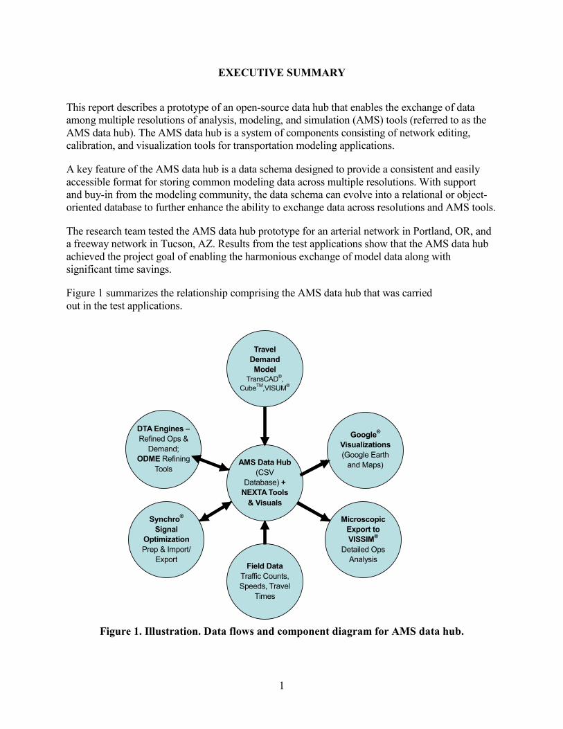
This report describes a prototype of an open-source data hub that enables the exchange of data among multiple resolutions of analysis, modeling, and simulation (AMS) tools (referred to as the AMS data hub). The AMS data hub is a system of components consisting of network editing, calibration, and visualization tools for transportation modeling applications.

A key feature of the AMS data hub is a data schema designed to provide a consistent and easily accessible format for storing common modeling data across multiple resolutions. With support and buy-in from the modeling community, the data schema can evolve into a relational or object-oriented database to further enhance the ability to exchange data across resolutions and AMS tools.

The research team tested the AMS data hub prototype for an arterial network in Portland, OR, and a freeway network in Tucson, AZ. Results from the test applications show that the AMS data hub achieved the project goal of enabling the harmonious exchange of model data along with significant time savings.

Figure 1 summarizes the relationship comprising the AMS data hub that was carried out in the test applications.

Figure 1. Illustration. Data flows and component diagram for AMS data hub.

Synchro® Signal

Optimization Prep & Import/

Export

Microscopic Export to VISSIM®

Detailed Ops Analysis

Travel Demand Model

TransCAD®, CubeTM,VISUM®

AMS Data Hub (CSV

Database) + NEXTA Tools

& Visuals

DTA Engines – Refined Ops &

Demand; ODME Refining

Tools

Google® Visualizations (Google Earth

and Maps)

Field Data

Traffic Counts, Speeds, Travel

Times

2

Specific benefits of the AMS data hub include the following:

• Capacity to quickly transfer most common travel demand models (TDMs) (i.e., TransCAD®, Cube VoyagerTM, and PTV Visum®) into mesoscopic dynamic traffic assignment (DTA) resolution for enhanced operational evaluations.

• Tools to adjust network, demand, and signal timing to facilitate quality DTA evaluations (portable to multiple DTA engines such as DTALite, Dynamic Urban Systems for Transportation (DynusT), and Dynamic Network Assignment-Simulation Model for Advanced Road Telematics (DynaSmart)).

• Origin-destination matrix estimation (ODME) to calibrate model volumes to field counts.

• Tools and export/import utilities with signal timing optimization tool (Synchro®) to build confidence in signal timing plans for DTA and microsimulation use.

• Import/export tools from the data hub to a common microsimulation tool (PTV Vissim®).

Results from the test application show significant time savings by using the AMS data hub compared to traditional ad hoc/manual methods. The most significant time savings are associated with network import functionality, creation of subarea origin-destination (O-D) matrices, automatic generation of signal timing for planning networks, and link volume calibration.

Table 1 summarizes the travel savings by component based on the results of the test applications, which reflect an 80 percent time savings.

Table 1. Estimated time saving from AMS data hub.

Component Without AMS

Data Hub With AMS Data Hub

Network import—Export, edit, and import network 8–10 h 1–2 h Intersection control inference—Edit control type for all nodes 6–8 h 4–6 h Subarea O-D matrices—Aggregate path flows at boundary 8–16 h < 0.5 h Convert connectors to side streets—Add new nodes, delete links, etc. 1–2 h < 0.5 h Signal timing with the quick estimation method (QEM)—Initial timings for intersections 6–8 h < 0.5 h ODME—Prepare field data and running ODME 6–8 h 2–3 h Total 35–52 h 7–11 h

3

Both the concept and interim tool demonstrations have been well received by the Portland Metro and Pima Association of Governments (PAG), which are the respective model agencies for the test applications. Portland Metro, in particular, has faced challenges with cross resolution modeling between macroscopic and mesoscopic tools. Their insights and requests, along with those of other professionals, have shaped the tools and functionality of the proof of concept AMS data hub tool. For example, Portland Metro expressed a strong desire to generate realistic signal timing plans and import them into the data hub (using Synchro®) for use with DTA. Portland Metro views signal timing as a key component to improving the realism of traffic assignments and results from DTA.

While this report discusses the integration of the AMS data hub for specific software tools to cross resolutions, the hub is intended to be an open source and customizable to support a wide variety of software tools. This is not an endorsement or recommendation of the specific software tools linked through this proof of concept, but rather a realistic test case for transferring data to support representative transportation analysis needs.

5

INTRODUCTION

The increasing complexity and interrelationship of transportation issues such as congestion, safety, emissions, accessibility, and mobility intensifies the need for practitioners to produce modeling results at multiple levels of resolution across multiple domains. Yet, no single AMS tool exists to answer the complex, multifaceted problems facing agency managers and elected officials. Often, gaps between data needs and capabilities prevent agencies from confidently addressing the problem at hand. Transportation Research Board’s Special Report 288 highlights the importance of applying the right tool for the right job by stating, “Travel forecasting tools...should be appropriate for the nature of the questions being posed by its constituent jurisdictions and the types of analysis being conducted.”(pg. 3)(1)

Given the multi-resolution nature of U.S. transportation problems, there remains an outstanding need to develop tools, guidelines, and approaches to effectively integrate a range of AMS tools. Planners and engineers have, at some level, integrated AMS tools for many years through the transcription of inputs and outputs, either manually or through customized utility programs. For example, traditional four-step regional TDM results are often postprocessed to develop turning movement counts which are then manually input into a deterministic Highway Capacity Manual (HCM)-method based model to arrive at intersection level performance measures such as level of service or volume-to-capacity (V/C) ratio.(2)

Drawbacks with this manual approach to integrated modeling include the following:

• It is time consuming and resource intensive.

• The accuracy of the results is likely subject to the constraints of the genesis model and its input data.

• It requires the user to understand the strengths and limitations of multiple modeling tools, either by their nature (resolution, domain, etc.) or as a result of software assumptions and algorithms that drive the results.

• It lacks the ability to interrelate the two-way effects of supply (network capacity and performance) and demand (volume, route, mode, departure time, etc.).

AMS tools primarily exist to address a single resolution or domain, such as solving large-scale transportation problems with coarse resolution or solving small-scale problems with fine details.(3) The integration of these models has historically been ad hoc in nature, offering data transfers within or between models or model resolutions in response to specific project needs. The problem with this approach is the lack of a framework or guidance to allow smaller integration efforts to fit together in a larger, collective body of work. Consistency and simplicity in model integration would enhance practitioner understanding and ease of use when integrating models.

6

CHARACTERISTICS OF EFFECTIVE INTEGRATION

The effective integration of AMS tools requires enhanced, reliable data sources, as well as informed well-trained users with a clear analytic objective typically defined by policy or decisionmakers to complement the multi-resolution models. Figure 2 illustrates a concept for integrating multiple AMS models and their relationships with data sources and decisionmakers.

Figure 2. Flowchart. Implementation of a conceptual integrated AMS tool.

It is important to note that effective integration of AMS tools requires more than seamlessly and accurately linking multiple model resolutions/domains together. Effective integration will require the following:(4)

• The availability and linking of key data sources as more advanced models are developed (activity-based, trip chaining, or real-time traffic counts or signal logic).

• Enhanced knowledge documentation and transfer to allow an understanding of key assumptions, limitations, and strengths of each modeling domain and resolution.

• Sufficient analysis demands and time to allow users to maintain and advance the skill sets needed to perform integrated modeling tasks.

• Sufficient computing power/hardware to efficiently complete desired integrated analysis.

7

MARKET DEMAND FOR INTEGRATION TOOLS

Demand for integrated modeling across multiple domains and resolutions are growing. Currently, software vendors, universities, and public agencies are developing approaches to accomplish model linkages and data transfers, but many are ad hoc in nature. A survey conducted as part of NCHRP 8-36 Task 90 indicated that the majority of users associated with integrated corridor management had already linked or were planning to link in the near future their regional demand planning model to a network simulation tool to perform time-dependent traffic assignments.(4) A one-way link between the coarser four-step TDM and a mesoscopic DTA or microsimulation model was by far the most common linkage cited within the surveyed agencies. Respondents who did not plan to integrate their planning and simulation models in the near future were discouraged by the difficulties in designing the data exchange mechanism.

Surveyed agencies identified the following common challenges to effectively integrate their planning (regional demand) models and network simulation tools (DTA or microsimulation):(4)

• Fitting or estimating O-D demand to link counts for calibration and validation. The problem is magnified when adjusted for future year scenarios.

• Network loading differences in that aggregated transportation analysis zone (TAZ) level data and connectors must be disaggregated to support actual entry points to a network (driveway, parking lot, etc.) within a microsimulation model.

• Adequate processing power and hardware to support the integrated modeling analysis.

NCHRP 8-36 Task 90 mainly focuses on system and congestion management as well as identifying capacity improvement projects through the lens of traffic operations.(4) It is important to recognize that effective integration of AMS tools must branch across multiple types of transportation disciplines. The need for linking operational performance measures with land use, environmental/emissions, safety, cost-benefit, and human factors models is paramount to supporting increasingly complex policy decisions within surface transportation.

9

MULTI-RESOLUTION AMS TOOL INTEGRATION

INTRODUCTION

Existing AMS tools have the capability to meet the needs of specific and relatively simplistic activities performed by different agencies. However, these tools have limited capacity to replicate complex system performance across different domains. For example, macroscopic TDMs are incapable of modeling detailed signal control, making them unsuitable to model traffic management and control alternatives. Running speed is a constraint for large networks in a microscopic simulation model. Real-time information and simulation of nonrecurring events are only available in the DTA and simulation models. Table 2 provides a high-level overview of AMS capabilities.

Table 2. Capabilities of AMS tools.

Domains

Capable of Replicating the

System Performance Running Speed

Receive Real-Time Information and

Simulate Nonrecurring

Events Macroscopic TDMs Yes on planning level

network Reasonable running speed for large network

No

Mesoscopic DTA models

Yes on subarea network level

Longer than macroscopic TDM

Yes

Microscopic simulation models

Yes on small network Requires significant running time for large networks

Yes

Activity-based models

Possible, calibration is resource intensive

Slow to medium No

Static deterministic programs

Yes on nodes and link level

Fast No

Safety Still developing Fast No Land use models Possible, calibration is

resource intensive Slow to medium No; typically

modeled for 5 years Emissions Yes Fast No

Although it is not suggested to use a single model across purposes for different domains, transportation models can be integrated on many levels because most of these domains are correlated with others on multiple dimensions. Figure 3 illustrates possible integration links between multiple AMS domains in transportation. The user may need to perform an integrated process when a comprehensive and complex transportation analysis is needed. The software tools for most of the integration links between the model domains in figure 3 are either unavailable, still in the research/development phase, or can be purchased as proprietary software programs. In many cases, users need to manually edit or create their own utility tools for integration purposes.

10

Figure 3. Illustration. Level of aggregation for various AMS tool domains.

USE CASES

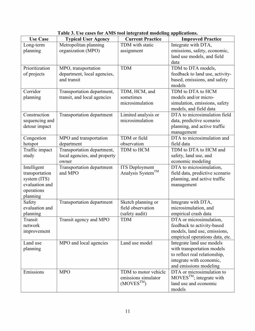
Several existing example use cases pertain to supporting transportation decisionmaking to solve complex challenges facing the transportation system. These challenges are multi-modal and diverse by geographic location. Temporal elements have multiple interrelated influences on the system including traffic demand, transportation capacity/supply, economic market forces, land use allocations and decisions, environmental conditions, and the desire to reduce crash frequency, to name a few. Table 3 presents a summary list of example use cases, typical user agency(s) that may be involved, current practice, and improved practice. The improved practice should be driven by the development and use of the AMS data hub.

11

Table 3. Use cases for AMS tool integrated modeling applications. Use Case Typical User Agency Current Practice Improved Practice

Long-term planning

Metropolitan planning organization (MPO)

TDM with static assignment

Integrate with DTA, emissions, safety, economic, land use models, and field data

Prioritization of projects

MPO, transportation department, local agencies, and transit

TDM TDM to DTA models, feedback to land use, activity-based, emissions, and safety models

Corridor planning

Transportation department, transit, and local agencies

TDM, HCM, and sometimes microsimulation

TDM to DTA to HCM models and/or micro-simulation, emissions, safety models, and field data

Construction sequencing and detour impact

Transportation department Limited analysis or microsimulation

DTA to microsimulation field data, predictive scenario planning, and active traffic management

Congestion hotspot

MPO and transportation department

TDM or field observation

DTA to microsimulation and field data

Traffic impact study

Transportation department, local agencies, and property owner

TDM to HCM TDM to DTA to HCM and safety, land use, and economic modeling

Intelligent transportation system (ITS) evaluation and operations planning

Transportation department and MPO

ITS Deployment Analysis SystemTM

DTA to microsimulation, field data, predictive scenario planning, and active traffic management

Safety evaluation and planning

Transportation department Sketch planning or field observation (safety audit)

Integrate with DTA, microsimulation, and empirical crash data

Transit network improvement

Transit agency and MPO TDM DTA or microsimulation, feedback to activity-based models, land use, emissions, empirical operations data, etc.

Land use planning

MPO and local agencies Land use model Integrate land use models with transportation models to reflect real relationship, integrate with economic, and emissions modeling

Emissions MPO TDM to motor vehicle emissions simulator (MOVESTM)

DTA or microsimulation to MOVESTM; integrate with land use and economic models

12

Travel model update

MPO Household travel survey, ad hoc integration of validation data from Census, traffic counts, and transit counts

Direct integration of estimation and validation data

NEEDED CAPABILITIES FOR EFFECTIVE MODEL INTEGRATION

A review of AMS tools and modeling practices has shown that current integrated modeling practices in transportation are mostly ad hoc and relatively inefficient. Inherent challenges to the modeling process include data constraints and inefficiencies, interoperability, calibration/validation, and adequate modeling behavioral response/feedback.

Data Constraints and Inefficiencies

Each stand-alone model program generally has sufficient data management techniques; however, each model program generally has a unique data format that impedes the ability to seamlessly integrate with other software programs. Effective model integration must bring diverse datasets into conformity. Currently, some users are developing ad hoc tools for integration. The lack of clear guidance and data standards is a barrier to entry for resource-constrained agencies that want to apply integrated modeling techniques. The following subsections provide additional detail regarding data constraints.

Data Availability

The types of input data required are often not readily available to modelers or are difficult to obtain, particularly for arterial streets and freeway off-ramps. A wave of new data sources, particularly probe-based data sources such as automatic vehicle identification, Bluetooth®, and data from private vendors along with real-time data from traffic signal controllers are becoming increasingly available for use in transportation modeling; however, these data sources are not yet widely integrated into standard modeling practices and still require significant labor resources to compile, postprocess, error check, and convert to a useful format.

Data Quality

Detector failure rates have been found to be as high as 60 percent, nearly double the 30 percent failure rate that is frequently cited as the average condition.(5) Poor data quality requires more time for scrubbing raw sensor data and raises questions about the credibility of modeling results.

Data Format

The lack of standardized data formats for common elements such as demand data (i.e., O-D, turning movement, vehicle trajectories, etc.), junction control data (i.e., signal timing), and, to a lesser extent, roadway network data requires manual manipulation or customization of utility tools to interface between models. This increases the risk of error in transposing data inputs. The

13

additional effort also takes away from time that could be spent on calibrating/validating, running additional scenarios, and performing sensitivity tests.

Many AMS tools have proprietary components that are encumbered by copyrights or other restrictions. These limitations create impediments for exchanging data across independent software packages and require the development and application of individual utility tools.

Data Exchange

It is important to standardize data exchange between tools at different levels of resolution in order to fully integrate multiple stand-alone models or simulation programs. An open standard would enhance the interoperability of analytical/simulation tools to coordinate and work together in a common (virtual) environment. This ability requires the cross resolution model integration architecture to be built on a common understanding of the transportation network, traffic demand, traffic control devices, and traffic sensor data.

System Coupling

Although a full integration approach within a single platform is desirable for cross resolution modeling, it requires a common data model and single-user interface for geographic information system (GIS) and other data analysis software. Thus, it is more practical to develop a future integrated modeling approach using either a loose coupling approach or a tight coupling approach. The utility tools serving the transfer of data files between different resolutions of common models need to be well defined and designed in order to be scalable, modular, interoperable, and extendable. Individual models should be developed on a modular basis so that each module can perform its function and be easily connected and extended to meet future modeling needs.

Interoperability

Software developers are enhancing the functionality of their suites of programs to enable integrated and cross resolution modeling to act as a one-stop shop for modeling needs. Examples include PTV Visum/PTV Vissim® by PTV Group®, TransCAD®/TransModeler® by Caliper®, and Aimsun® by Transport Simulation Systems®. However, given the lack of industry-wide data standards and protocols, it is generally not feasible from a time and resource perspective for practitioners to work across multiple software-developer packages, and even if they did, the process would be far from seamless. This underscores the driving need to establish guidelines, standards, and protocols to address data handling and exchange.

CALIBRATION/VALIDATION

Few guidance or support tools exist for the calibration/validation of performance at a network level and for cross resolution model integration. Most validation is generally performed by qualitatively assessing the results and output for reasonableness. To the extent quantitative validation is performed, it is generally based on link or turning movement volumes. It is often difficult to validate performance measures such as travel time and route choice given the lack of available data, particularly when broken down for individual O-D pairs and routes.

14

The lack of calibration and validation can lead to a credibility issue with the public and decisionmakers and result in agencies shying away from applying data-driven models.

BEHAVIORAL RESPONSE

One of the most significant gaps in the functionality of current models is the lack of behavioral response associated with congestion, pricing, and traveler information (and other demand management strategies). Transportation models in many cases require significant manipulation and calibration to produce reasonable results for networks that are oversaturated and/or include demand management strategies that affect travelers’ choice of mode, departure time, and route. By only focusing on the supply side, many transportation analyses do not reflect the true effects of operating conditions, particularly when it comes to examining performance over multiple days for the purposes of estimating reliability. Ongoing research efforts are addressing this shortcoming and are expected to produce enhanced modeling tools and techniques that will establish a foundation for the future state-of-the-practice. As such, the development of standards, tools, and guidance as part of this project should look ahead to meet future modeling needs, not just current practice, which may soon be outdated in some cases.

15

AMS DATA HUB CONCEPT OF OPERATIONS

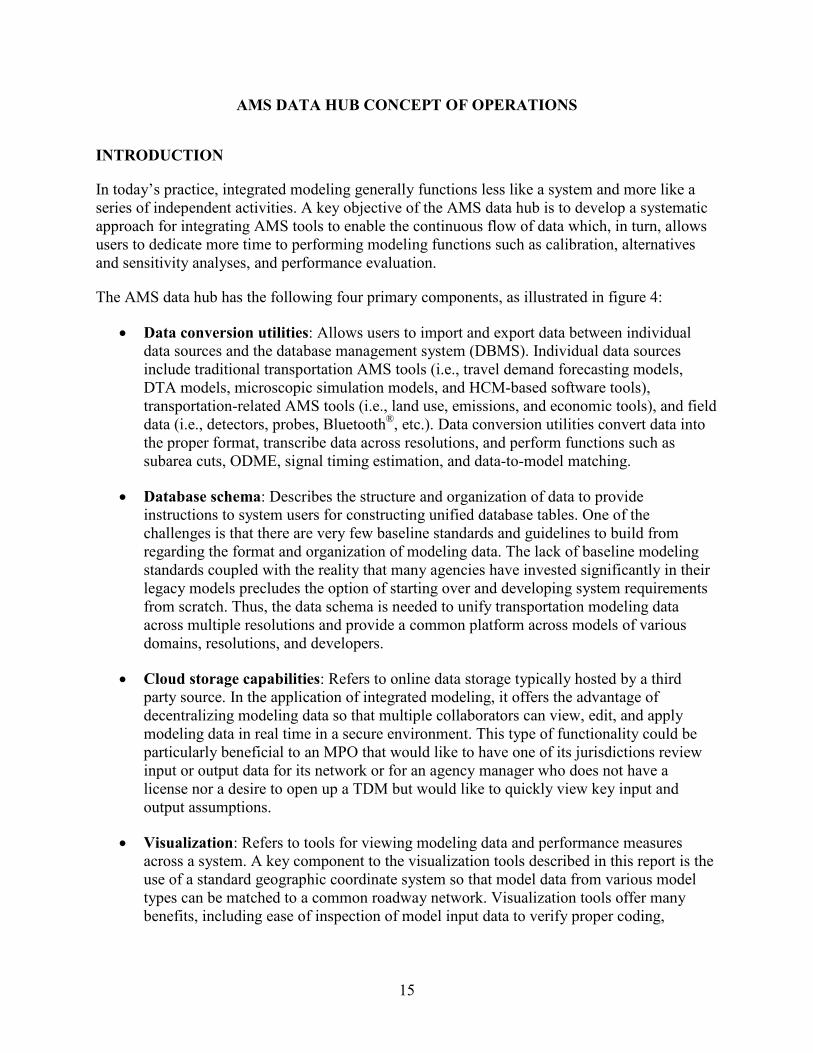
INTRODUCTION

In today’s practice, integrated modeling generally functions less like a system and more like a series of independent activities. A key objective of the AMS data hub is to develop a systematic approach for integrating AMS tools to enable the continuous flow of data which, in turn, allows users to dedicate more time to performing modeling functions such as calibration, alternatives and sensitivity analyses, and performance evaluation.

The AMS data hub has the following four primary components, as illustrated in figure 4:

• Data conversion utilities: Allows users to import and export data between individual data sources and the database management system (DBMS). Individual data sources include traditional transportation AMS tools (i.e., travel demand forecasting models, DTA models, microscopic simulation models, and HCM-based software tools), transportation-related AMS tools (i.e., land use, emissions, and economic tools), and field data (i.e., detectors, probes, Bluetooth®, etc.). Data conversion utilities convert data into the proper format, transcribe data across resolutions, and perform functions such as subarea cuts, ODME, signal timing estimation, and data-to-model matching.

• Database schema: Describes the structure and organization of data to provide instructions to system users for constructing unified database tables. One of the challenges is that there are very few baseline standards and guidelines to build from regarding the format and organization of modeling data. The lack of baseline modeling standards coupled with the reality that many agencies have invested significantly in their legacy models precludes the option of starting over and developing system requirements from scratch. Thus, the data schema is needed to unify transportation modeling data across multiple resolutions and provide a common platform across models of various domains, resolutions, and developers.

• Cloud storage capabilities: Refers to online data storage typically hosted by a third party source. In the application of integrated modeling, it offers the advantage of decentralizing modeling data so that multiple collaborators can view, edit, and apply modeling data in real time in a secure environment. This type of functionality could be particularly beneficial to an MPO that would like to have one of its jurisdictions review input or output data for its network or for an agency manager who does not have a license nor a desire to open up a TDM but would like to quickly view key input and output assumptions.

• Visualization: Refers to tools for viewing modeling data and performance measures across a system. A key component to the visualization tools described in this report is the use of a standard geographic coordinate system so that model data from various model types can be matched to a common roadway network. Visualization tools offer many benefits, including ease of inspection of model input data to verify proper coding,

16

identification of hotspots across a network, and communication of information to lay audiences.

This report provides a high-level overview of a recommended database schema for unifying modeling data across commonly used AMS tools. Figure 4 provides an overview on the proposed software architecture by illustrating the information data flow procedures between different components.

The following sections describe each component in detail, including its primary function, internal relationship with other components, key characteristics, and operation environment.

Figure 4. Illustration. AMS data hub architecture.

17

18

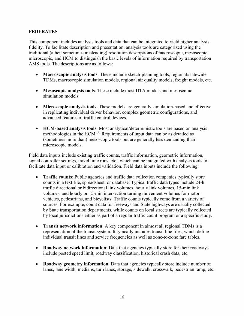
FEDERATES

This component includes analysis tools and data that can be integrated to yield higher analysis fidelity. To facilitate description and presentation, analysis tools are categorized using the traditional (albeit sometimes misleading) resolution descriptions of macroscopic, mesoscopic, microscopic, and HCM to distinguish the basic levels of information required by transportation AMS tools. The descriptions are as follows:

• Macroscopic analysis tools: These include sketch-planning tools, regional/statewide TDMs, macroscopic simulation models, regional air quality models, freight models, etc.

• Mesoscopic analysis tools: These include most DTA models and mesoscopic simulation models.

• Microscopic analysis tools: These models are generally simulation-based and effective in replicating individual driver behavior, complex geometric configurations, and advanced features of traffic control devices.

• HCM-based analysis tools: Most analytical/deterministic tools are based on analysis methodologies in the HCM.(2) Requirements of input data can be as detailed as (sometimes more than) mesoscopic tools but are generally less demanding than microscopic models.

Field data inputs include existing traffic counts, traffic information, geometric information, signal controller settings, travel time runs, etc., which can be integrated with analysis tools to facilitate data input or calibration and validation. Field data inputs include the following:

• Traffic counts: Public agencies and traffic data collection companies typically store counts in a text file, spreadsheet, or database. Typical traffic data types include 24-h traffic directional or bidirectional link volumes, hourly link volumes, 15-min link volumes, and hourly or 15-min intersection turning movement volumes for motor vehicles, pedestrians, and bicyclists. Traffic counts typically come from a variety of sources. For example, count data for freeways and State highways are usually collected by State transportation departments, while counts on local streets are typically collected by local jurisdictions either as part of a regular traffic count program or a specific study.

• Transit network information: A key component in almost all regional TDMs is a representation of the transit system. It typically includes transit line files, which define individual transit lines and service frequencies as well as zone-to-zone fare tables.

• Roadway network information: Data that agencies typically store for their roadways include posted speed limit, roadway classification, historical crash data, etc.

• Roadway geometry information: Data that agencies typically store include number of lanes, lane width, medians, turn lanes, storage, sidewalk, crosswalk, pedestrian ramp, etc.

19

• Signal controller settings: Most controllers have information regarding rings, barriers, phases (movements and duration, sequence, etc.), coordination (offset, cycle length, etc.), time settings, detectors, time of day plan, etc.

• Travel time runs: Corridor travel time runs can be collected by probe cars or Bluetooth® devices.

Note that this report does not provide detailed information on transportation-related analysis tools such as land use, emissions, and safety models. The AMS data hub concept can be extended in the future to include other related models.

DATA CONVERSION TOOLBOX

The conversion toolbox is one of the core components of the AMS data hub. Within the current state of the practice, many conversions are required to transfer data among analysis tools. Over time, it is likely that the conversion toolbox will become less and less critical as analysis tools adopt the unified data structure and have built-in capability to import/export AMS data hub compatible format. However, for near-term applications, the conversion toolbox is essential. This section provides data hub users with a better understanding of underlying multi-resolution modeling elements, automated processes of disaggregating and aggregating data across different resolutions, and value added and data mining support tools such as subarea O-D demand matrix updating and sensor data management.

Table 4 provides a summary of typical modeling components used at different resolutions of transportation modeling and simulation tools.

20

Table 4. Summary of typical transportation AMS data types.

Data Type

Data Resolution Macroscopic

Regional Planning Models (Including

Agent-Based Demand and Land

Use Models) Mesoscopic DTA

Microscopic Traffic Simulation, Travel

Demand, and Highway Capacity Analysis

Tools Node Coordinates turning

movement permission and restriction

Movement-specific capacity

Turning volume and signal timing plan

Link Upstream node, downstream node, length, link capacity, and number of lanes

Number of left-turn and right-turn bays and length of bays

Lane-to-lane connectors at intersections and detailed geometry of lanes

Vehicle demand Household, population, employment of traffic analysis zones, parcel-level household data for activity origins and destinations, and peak hour O-D demand matrix by different trip purposes and vehicle types

Time-dependent departure time profile and vehicle paths under different traveler information provision strategies

Node-specific turning movement and vehicle routing plan in the subarea

Transit demand Transit network with connectors from zone centroids

Number of transit vehicles on network

Individual transit stops with walk access connectors from land parcels

Link measure of effectiveness (MOE) output from simulators/ models

Peak hour end-to-end travel time and accessibility, link speed, and flow rate

Link-based time-dependent flow rates and queue evolution

Second-by-second lane-by-lane vehicle trajectory

Observed sensor measurements

Peak hour link count and end-to-end travel time

Time-dependent loop detector data such as speed, flow, occupancy, and time- dependent travel time

High-fidelity vehicle trajectory data (e.g., Next Generation Simulation)

21

To facilitate the seamless cross resolution modeling practice and improve the modeling accuracy of simulation and planning models, the AMS data hub should consider the following guiding principles:

• Embed a spatial data representation: The AMS data hub should allow the user (e.g., MPO planners and traffic engineers) to export shared datasets from the data hub to a GIS environment.

• Recognize cross resolution dependencies between elements at different resolutions: To minimize the complexity in managing cross resolution data dependencies, the AMS data hub should first provide full coverage of modeling elements at the mesoscopic level and then streamline the compatible data access interfaces that traverse the boundaries of mesoscopic to macroscopic and mesoscopic to microscopic representations, including network, traffic demand, and vehicle trip elements.

• Provide bidirectional cross resolution modeling (disaggregation and aggregation): Disaggregation involves the breakdown of regional network and demand elements from macroscopic modeling methods to fine-grained subarea representations used in microscopic simulation systems. Aggregation involves the compilation of simulation results from a high-fidelity traffic simulator to network-level measures for macroscopic traffic demand forecasting tools such as activity-based/land use models. This bidirectional cross resolution data flow offers a strong support to integrate traffic demand/supply in a feedback loop.

• Provide additional MOEs such as reliability, safety, and sustainability for region-wide and project-level traffic impact analysis: Cross domain modeling has the potential to bridge the gap between congestion-oriented traffic assignment/simulation models with the other critical evaluation criteria such as safety, reliability or sustainability. Table 5 details the steps for information propagation and exchange in cross domain applications.

• Facilitate the use of emerging mobile data sources, innovative data acquisition methods, and collaborative data management: Challenges in handling multiple sources with different formats and varying data quality include mapping and transforming raw loop/Bluetooth®/Global Positioning System sensor data to travel time and flow volume information on geo-coded transportation modeling networks used in transportation planning and simulation and constructing a real-world data environment to enable accurate offline or online traffic simulation with seamless connections to real-world observations, incident, and work zone data.

• Include functionality to streamline calibration/validation: A key benefit from data-model integration is to bring diverse sensor data sets into conformity and further improve the modeling accuracy. Additional software tools can be developed within the proposed data hub environment to establish a closer connection between field and model data and support real-time traffic management strategies such as the Connected Vehicle Initiative.

22

Table 5. Data flow for information propagation and exchange in cross domain applications.

Data Type

Data Resolution Macroscopic

Representation Mesoscopic

Representation Microscopic

Representation Domain application

Safety impact evaluation

Travel time reliability analysis

Emission impact studies

Output through data hub

Link volume (average annual daily traffic (AADT)) and congestion level

Time-dependent path flow pattern and link capacity variations under recurring conditions

Second-by-second lane-by-lane vehicle trajectory

Additional information from specific domain applications

AADT-based crash prediction formulas for different facility types

Link volume, capacity, and demand variations due to incidents, work zone, and severe weather conditions

Vehicle-specific power-to-emission conversion table

Additional MOEs

Peak hour and daily crash rates and capacity reduction

End-to-end travel time reliability measures under recurring and non-recurring conditions

Regional- and project-level emissions estimates and sustainability analysis

Network EXplorer for Traffic Analysis (NeXTA) version 3 is the prototype implementation of the AMS data hub that was developed based on the guiding principles highlighted in this section. It houses various conversion tools and provides a visualization as well as connection with the cloud storage. The following conversion tools are currently embedded in NeXTA:

• From TDMs (Cube VoyagerTM, PTV Visum®, and TransCAD®) to NeXTA.

• From DynaSmart-PTM-P and DynusTTM to NeXTA.

• From Synchro® to NeXTA.

• From link counts to NeXTA.

• From NeXTA to Synchro®.

• From NeXTA to PTV Vissim®.

• From NeXTA to Google Fusion Tables®.

Other functions provided by NeXTA include the following:

• DTALite: A mesoscopic DTA engine called DTALite that can be run directly from within NeXTA. DTALite is a mesoscopic simulation-assignment framework that uses a computationally simple but theoretically rigorous traffic queuing model in its simulation engine. Its greatest strength over other DTA software is its ability to model a large network with a minimal set of data and computing resources.

23

• Subarea: Users can define a small study area, and NeXTA automatically performs all necessary steps to create an independent network of the subarea that is ready for further analysis.

• ODME: This technique is used to adjust demand patterns in a network to better approximate observed traffic conditions (e.g. time-dependent link volume). It is an iterative process that assigns trips to paths in a network, compares observed and simulated link volumes/counts, adjusts the input demand data, and moves to the next iteration where the trips are reassigned. With a simple click and minimal user input, NeXTA invokes DTALite in the background and automatically completes the iteration.

DATABASE SCHEMA

This section describes a unified data structure that facilitates input/output data conversion in the short term and promotes data consistency and exchange in the long term.

The component diagram shown in figure 4 illustrates the relationship of the series of tables in the proposed database schema: zones, nodes, links, demands, transit, household travel surveys, travel model outputs, MOEs, scenarios, signal control, vehicle trajectories, and configuration.

A few key points regarding the organization of the data hub tables are as follows:

• The arrow indicates the parent-child relationship. For example, a zone can have one or more links; a link can have nodes, demands, and performance measures; a node can have a signal, stop control, or roundabout; etc.

• The signals and trajectory tables are currently applicable only to mesoscopic and microscopic resolutions.

• As previously mentioned, HCM-based tools fall between the mesoscopic and microscopic categories. As such, some table data are applicable to the HCM-based tools.

• The configuration table is independent of the other tables.

Advantages of the database schema are as follows:

• The database is software neutral.

• The initially proposed database tables can be expanded in the future.

• Software can be configured to read all or a subset of parameters in a table.

• A software vendor can add field parameters that are specific to its product.

• Links and nodes are geo-coded and thus more easily integrate with GIS and other visualizers such as Google Maps®.

24

• Since the data structure is transparent and openly defined, it can readily be scrutinized, tested, and enhanced.

• The database can serve as a platform to encourage the development of analysis tools and visualization tools, especially from small software vendors and researchers.

• The database moves the practice of integrated modeling toward a standard for how modeling data should be stored and shared as opposed to the current ad-hoc practice which varies across users and agencies.

One disadvantage of such an overarching unified data schema is its size, which has an adverse effect on computational speed and efficiency. The data structure is understandably large in order to accommodate analysis models in various resolutions (i.e., a single intersection analysis using the HCM method would utilize only a small portion of the data structure).

A description of each of the components of the database schema is provided in appendix B of this report. The description is general in nature, and the database schema can be implemented in multiple ways. Regardless of the format, the AMS data hub must accommodate a wide variety of data types, some of which are quite complex (see table 6). Examples of data types are as follows:

Simple data types:

• Strings: Alphanumeric fields that are typically short (less than 200 characters) and contain descriptive or type data.

• Integers: Used for floating point numbers.

Complex data types:

• Coordinates: Used to specify geographic locations of points such as nodes. A series of coordinates is used to define a shape such as a link or a zone boundary. Coordinates are specified in a predefined system (e.g., latitude/longitude or universal transverse Mercator (UTM)).

• Geometry: Needed to specify boundaries (in the case of zones) or paths (in the case of links).

The data type definitions in table 6 are proposed in the database schema.

25

Table 6. Data types.

Type Definition Range

Notes Minimum Maximum Int Signed 32-bit

integer value -2,147,483,648 2,147,483,647 Other possible integer types

(which are less often used): byte (8 bits), short int (16 bits), and long int (64 bits)

Double Double precision floating point number

-1.797e308 1.797e308 Used for most inputs that can take on any value, including fractional values

Enum Takes on one of several prespecified values

N/A N/A Used for categorical variables (e.g., facility type = freeway, arterial, ramp, etc.)

Bool Boolean value: true or false

N/A N/A N/A

String String of unicode characters

N/A N/A N/A

Extensible Markup Language (XML)

XML formatted field

N/A N/A Can alternately be defined as a string variable, but some DBMSs provide XML field definitions with special handling (e.g., the user may have to specify a validating schema)

Array n-dimensional array

N/A N/A An array of any simple type

Date/time Date and time value

N/A N/A N/A

Geometry Geometric object N/A N/A Can be a point, line segment, path, or polygon

User-defined

User-defined data object to hold complex data types

N/A N/A Some DBMSs allow user-defined objects, but these usually require an additional handling code to be written by the user

N/A = Not applicable. n = Number of dimensions in the subject array.

NeXTA version 3 is used for the test applications conducted for the AMS data hub. Its data structure is loosely based on the proposed data schema. To allow the most flexibility, readability, and compatibility with the open-source concept, NeXTA’s tables are currently stored in a series of comma-separated values (CSV) files. As a compromise, it lacks advanced capabilities such as table linkage, shared access, entry validation, etc., that are typically inherent in a database.

26

CLOUD STORAGE

Google Fusion Tables® is employed to demonstrate the benefits of cloud storage. Data uploaded to Google Fusion Tables® are stored on the Google® cloud server. The tables can be shared with many users. Google Fusion Tables® is free and provides many functions to work with and manipulate data. Since it is open source, there is a growing number of add-in tools developed by others and distributed freely. Figure 5 shows link and node data from a sample network that has been exported from NeXTA and uploaded to Google Fusion Tables®. Similarly, the network data can be downloaded from Google Fusion Tables® in CSV format and imported into NeXTA or other software.

©2012 Google Fusion Tables®

Figure 5. Screenshot. Google Fusion Tables® data exported from NeXTA.(6)

VISUALIZATION

Visualization is an increasingly important element of transportation analysis and should be an integral part of any AMS data hub. Analysts can apply several readily available visualization functions with Google Fusion Tables®. Figure 6 and Figure 7 illustrate two examples.

27

©2013 Google Maps®

Figure 6. Illustration. Example network plotted using Google Maps®.(7)

©2012 Google Fusion Tables®

Figure 7. Graph. Example scatter plot using Google Fusion Tables®.(8)

The NeXTA interface also has many useful visualization functions. Visual display of commonly used MOEs such as V/C ratio, speed, and queuing are readily available from one of the toolbars (see figure 8).

Figure 8. Illustration. NeXTA toolbar visualization options.

28

V/C Visualization

The V/C visualization view shows time-dependent V/C ratios for each link in the network. The color coding is user definable and allows for quantifying locations and durations of congestion in a network, as shown in figure 9.

Figure 9. Illustration. V/C ratio performance by link.

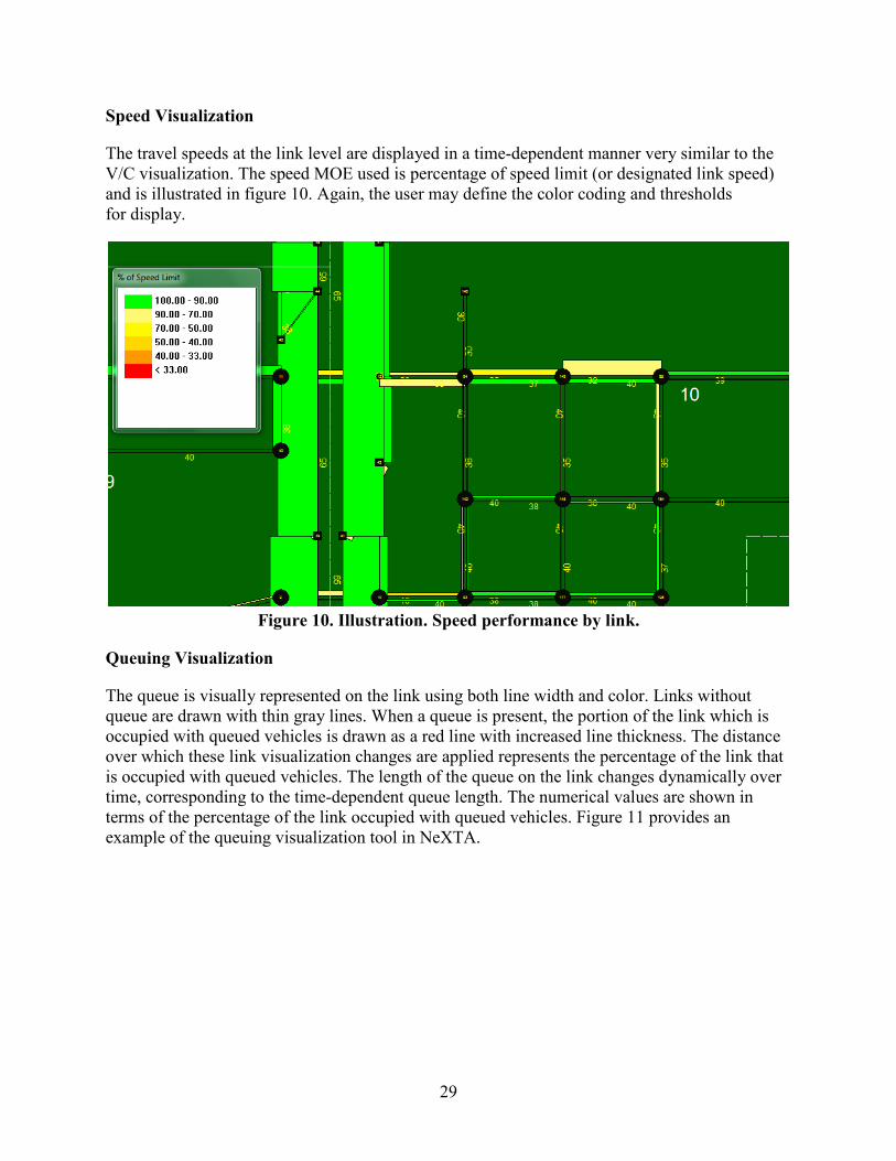
29

Speed Visualization

The travel speeds at the link level are displayed in a time-dependent manner very similar to the V/C visualization. The speed MOE used is percentage of speed limit (or designated link speed) and is illustrated in figure 10. Again, the user may define the color coding and thresholds for display.

Figure 10. Illustration. Speed performance by link.

Queuing Visualization

The queue is visually represented on the link using both line width and color. Links without queue are drawn with thin gray lines. When a queue is present, the portion of the link which is occupied with queued vehicles is drawn as a red line with increased line thickness. The distance over which these link visualization changes are applied represents the percentage of the link that is occupied with queued vehicles. The length of the queue on the link changes dynamically over time, corresponding to the time-dependent queue length. The numerical values are shown in terms of the percentage of the link occupied with queued vehicles. Figure 11 provides an example of the queuing visualization tool in NeXTA.

30

Figure 11. Illustration. Queuing performance by link.

NeXTA’s visualization tools also provide additional MOEs, some of which are more advanced and in the forefront of the transportation analysis practice. One of them is the path travel time reliability analysis tool, which is an advanced feature for investigating travel time reliability and sources of unreliability.

31

TEST NETWORK OVERVIEW

INTRODUCTION

The research team conducted two test applications using the AMS data hub prototype. The objective of the test application is to create seamless linkages between AMS tools and multiple resolutions. The test applications aim to replicate real-world analyses and enable alternatives analyses and scenario evaluations.

The two networks selected for testing are located in Tucson, AZ, and Portland, OR. These networks were chosen due to agency interest, availability of field data, and availability of AMS models. Additionally, the two networks collectively represent a freeway (Tucson, AZ) and arterial (Portland, OR) network.

DESCRIPTION OF TEST NETWORKS

Tucson, AZ, Test Network

The I-10 Casa Grande Tucson Highway traverses the northwestern and eastern portions of Pima County and is an important corridor serving Tucson commuters as well as interstate traffic. The Arizona Department of Transportation (ADOT), in conjunction with the Federal Highway Administration, has identified the need to reconstruct I-10 from milepost 247.5 to milepost 253.0 to increase the roadway capacity and to improve operational efficiency. As part of the planning process, a detailed traffic study is required to establish year 2040 traffic demands and capacity needs. The study should also recommend a construction sequencing strategy with the least impact to road users. This test application presents the application of the AMS data hub to address some of the project’s traffic questions.

Objectives of the Tucson, AZ, test application are as follows:

• Illustrate the functionality and workflow of NeXTA.

• Illustrate the application of the unified data format and AMS tool to a real-world problem.

• Demonstrate benefits of an integrated AMS approach over the traditional analysis approach.

• Identify future capacity requirements for the I-10 corridor.

• Evaluate optimal construction sequencing for the corridor and its interchanges.

Figure 12 depicts the study area, the I-10 corridor, and its interchanges (TIs). As shown, there are four existing interchanges within the study corridor. The I-10 mainline currently goes over the crossroads at the Ina Road, Sunset Road, and Ruthrauff Road TIs. The reconstruction will place the crossroads over I-10 and thus require complete closure of those three TIs.

32

Figure 12. Illustration. Tucson, AZ, test network and intersection geometry.

Input data for the Tucson, AZ, test application are summarized in table 7.

Table 7. Source data for Tucson, AZ, test application. Source Data Type AMS Tool Source

Regional TDM TransCAD® PAG 24-h segment counts, intersection turning movement counts, I-10 mainline speed data

N/A Collected by quality counts for ADOT

Regional Synchro® models Synchro® PAG N/A = Not applicable.

Portland, OR, Test Network

NW 185th Avenue is located in the center of Portland’s western suburbs and bisects Beaverton and Hillsboro. The population of both communities is rising and outpacing growth in the greater Portland metro area. NW 185th Avenue is one of the longest continuous north-south major arterials in western suburban Portland. This important link has largely commercial and residential adjacent land uses and carries an average daily traffic of 30,000 across a mostly five-lane cross section.

Figure 13 shows the limits of the NW 185th Avenue corridor and locations of traffic signals. Projected future vehicular volumes warrant widening NW 185th Avenue to seven lanes or more, but regional MPO livability policy dictates no roadway widening beyond five lanes. Thus, a time-dependent, capacity constrained evaluation is needed at the link level to provide an informed decision about the likely congestion impacts and route diversion to occur if NW 185th Avenue arterial is left at five lanes or if it is widened.

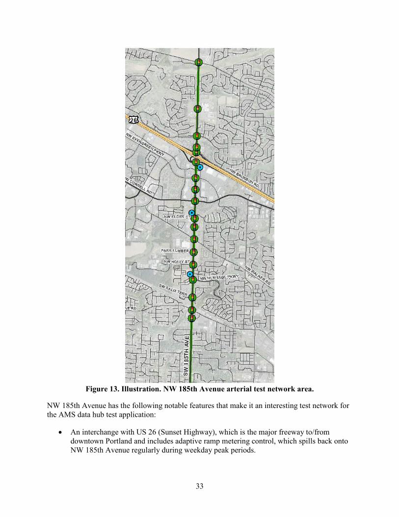
33

Figure 13. Illustration. NW 185th Avenue arterial test network area.

NW 185th Avenue has the following notable features that make it an interesting test network for the AMS data hub test application:

• An interchange with US 26 (Sunset Highway), which is the major freeway to/from downtown Portland and includes adaptive ramp metering control, which spills back onto NW 185th Avenue regularly during weekday peak periods.

34

• An at-grade light rail crossing (see Figure 14) projected to increase future train frequency beyond the 5-min or less current headways during peak periods, which creates more challenges for a congested network and particularly the major signalized intersection to the south of the light rail crossing.

• Regional shopping centers that draw heavy traffic volumes during weekends and holidays.

• Two high schools and two elementary schools, inducing variability in traffic peaking and at times significant pedestrian, bicycle, and transit demand.

• The corridor is a candidate for transit signal priority, truck signal priority, and adaptive signal control as advanced ITS solutions.

Photo Credit: Shaun Quayle, Kittelson & Associates

Figure 14. Photo. Light rail crossing on NW 185th Avenue.

For the purposes of this test application, a DTA evaluation is necessary at a larger subarea level to evaluate alternative routes due to sizing of the NW 185th Avenue arterial. For the deterministic or microsimulation evaluations, the team focused on the most congested portion of the network near the US 26 interchange, which is adjacent to the Tanasbourne regional shopping center where ramp meter spillback is most pronounced.

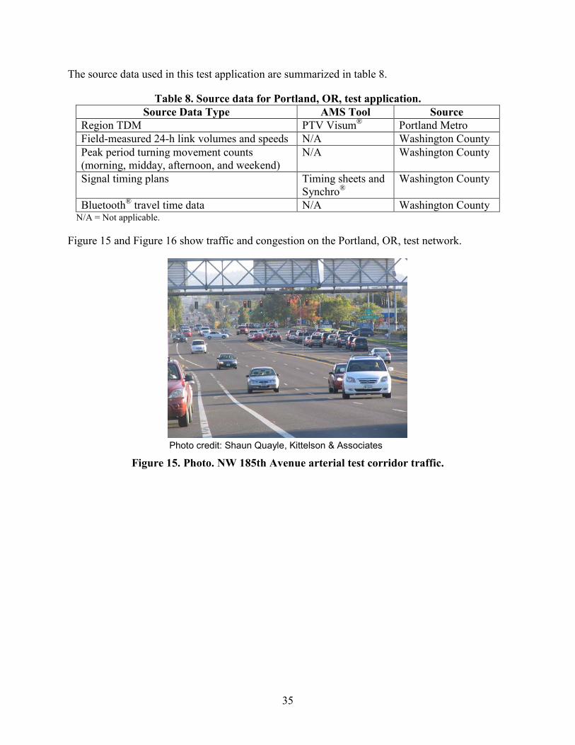
35

The source data used in this test application are summarized in table 8.

Table 8. Source data for Portland, OR, test application. Source Data Type AMS Tool Source

Region TDM PTV Visum® Portland Metro Field-measured 24-h link volumes and speeds N/A Washington County Peak period turning movement counts (morning, midday, afternoon, and weekend)

N/A Washington County

Signal timing plans Timing sheets and Synchro®

Washington County

Bluetooth® travel time data N/A Washington County N/A = Not applicable.

Figure 15 and Figure 16 show traffic and congestion on the Portland, OR, test network.

Photo credit: Shaun Quayle, Kittelson & Associates

Figure 15. Photo. NW 185th Avenue arterial test corridor traffic.

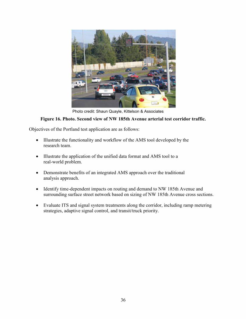
36

Photo credit: Shaun Quayle, Kittelson & Associates

Figure 16. Photo. Second view of NW 185th Avenue arterial test corridor traffic.

Objectives of the Portland test application are as follows:

• Illustrate the functionality and workflow of the AMS tool developed by the research team.

• Illustrate the application of the unified data format and AMS tool to a real-world problem.

• Demonstrate benefits of an integrated AMS approach over the traditional analysis approach.

• Identify time-dependent impacts on routing and demand to NW 185th Avenue and surrounding surface street network based on sizing of NW 185th Avenue cross sections.

• Evaluate ITS and signal system treatments along the corridor, including ramp metering strategies, adaptive signal control, and transit/truck priority.

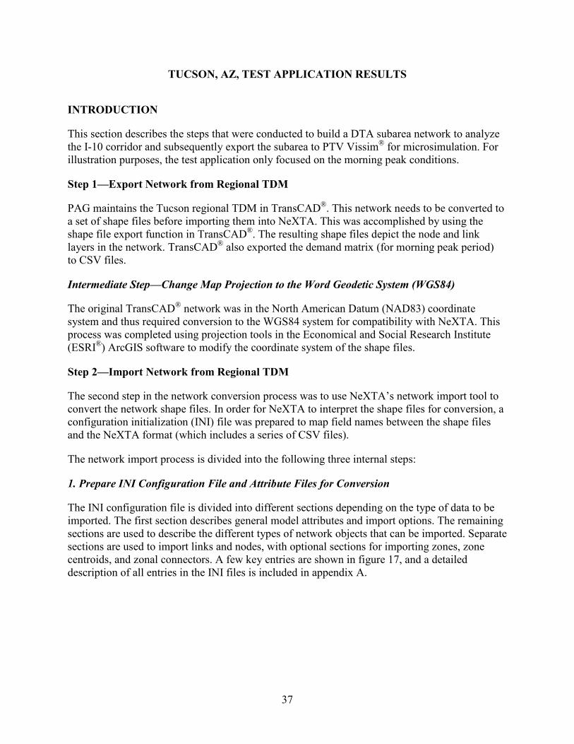
37

TUCSON, AZ, TEST APPLICATION RESULTS

INTRODUCTION

This section describes the steps that were conducted to build a DTA subarea network to analyze the I-10 corridor and subsequently export the subarea to PTV Vissim® for microsimulation. For illustration purposes, the test application only focused on the morning peak conditions.

Step 1—Export Network from Regional TDM

PAG maintains the Tucson regional TDM in TransCAD®. This network needs to be converted to a set of shape files before importing them into NeXTA. This was accomplished by using the shape file export function in TransCAD®. The resulting shape files depict the node and link layers in the network. TransCAD® also exported the demand matrix (for morning peak period) to CSV files.

Intermediate Step—Change Map Projection to the Word Geodetic System (WGS84)

The original TransCAD® network was in the North American Datum (NAD83) coordinate system and thus required conversion to the WGS84 system for compatibility with NeXTA. This process was completed using projection tools in the Economical and Social Research Institute (ESRI®) ArcGIS software to modify the coordinate system of the shape files.

Step 2—Import Network from Regional TDM

The second step in the network conversion process was to use NeXTA’s network import tool to convert the network shape files. In order for NeXTA to interpret the shape files for conversion, a configuration initialization (INI) file was prepared to map field names between the shape files and the NeXTA format (which includes a series of CSV files).

The network import process is divided into the following three internal steps:

1. Prepare INI Configuration File and Attribute Files for Conversion

The INI configuration file is divided into different sections depending on the type of data to be imported. The first section describes general model attributes and import options. The remaining sections are used to describe the different types of network objects that can be imported. Separate sections are used to import links and nodes, with optional sections for importing zones, zone centroids, and zonal connectors. A few key entries are shown in figure 17, and a detailed description of all entries in the INI files is included in appendix A.

38

Figure 17. Screenshot. Sample INI configuration file.

In figure 17, the variables on the left side of the equal sign are NeXTA’s field names, while the variables in quotation marks are field names in the TransCAD® shape files. Some of the fields imported from TransCAD® into NeXTA were from_node, to_node, street name, segment length, capacity, and speed limit.

Two additional attribute files that required preparation were the input_link_type.csv and input_node_control_type.csv. The input_link_type maps the link types in TransCAD® with the link types in NeXTA. Since the Tucson TDM does not contain traffic control data, NeXTA applied its default control types during conversion.

2. Use NeXTA’s Import Network Tool to Convert the Network

Starting with a new empty network project in NeXTA, the conversion process was initiated by selecting the INI file. After the successful conversion process, NeXTA displayed a file loading status window as shown in figure 18.

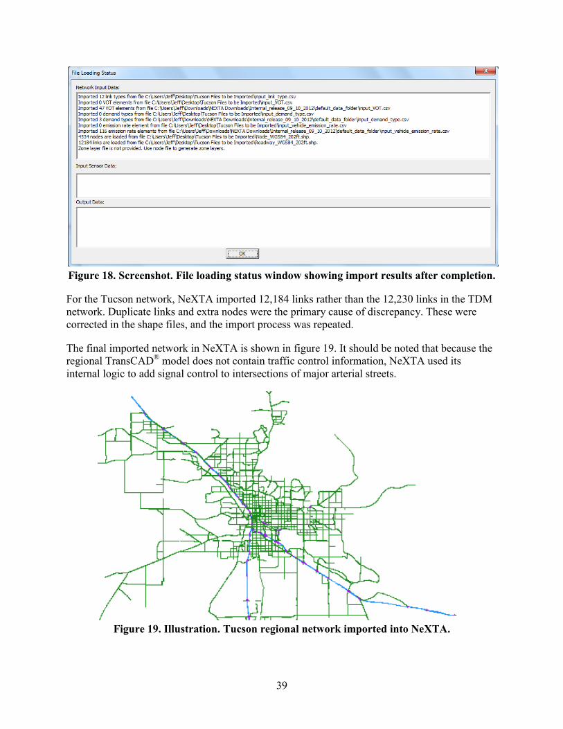
39

Figure 18. Screenshot. File loading status window showing import results after completion.

For the Tucson network, NeXTA imported 12,184 links rather than the 12,230 links in the TDM network. Duplicate links and extra nodes were the primary cause of discrepancy. These were corrected in the shape files, and the import process was repeated.

The final imported network in NeXTA is shown in figure 19. It should be noted that because the regional TransCAD® model does not contain traffic control information, NeXTA used its internal logic to add signal control to intersections of major arterial streets.

Figure 19. Illustration. Tucson regional network imported into NeXTA.

40

3. Save the New Network As a New Project File

The network was saved as a new transportation network project (.tnp) file.

Step 3—Read Demand Data from Regional TDM

Similar to the INI file, the input_demand_meta_data.csv file is used by NeXTA to find and read the O-D tables exported from TDMs. This metadata file requires several entries, but the relevant entries include the following:

• File name: “DA_GP.csv” is the O-D matrix for the morning period brought into NeXTA.

• Format: “Matrix” is the type of O-D matrix format for the Tucson test application.

• Start and end times: “Start_time” is minute 420 or 7 a.m., and the “End_time” is minute 540 or 9 a.m. The O-D matrix stores the number of trips between 7 a.m. and 9 a.m.

Step 4—Run Assignment with DTALite to Equilibrium

Before a subarea was created for more detailed analyses, DTA was performed with DTALite to ensure equilibrium network path flows and thus reasonable trips entering the subarea. Running the DTALite assignment engine requires editing the simulation settings in the input_scenario_settings.csv file and initiating the assignment engine (e.g., selecting simulation from one of the NeXTA toolbars).

DTALite is fairly efficient. For the Tucson regional network with 10 simulation runs for about 310,000 vehicles, DTALite took 5 min 22 s of computational time on an Intel® Core 2 Duo T7500 (2.2 GHz) with 3 GB RAM. It was determined that the average travel time was 14.67 min with an average trip length of 7.55 mi within the Tucson network.

Step 5—Cut a Subarea Within the Larger Model for More Detailed Analysis

To focus on the I-10 corridor from the Ina Road interchange to the Ruthrauff Road interchange, select link analyses were conducted, and it was determined that the study subarea needed to include one additional interchange to the north and three interchanges to the south. NeXTA simplifies the subarea creation process by automatically handling extraction of necessary nodes, links, zones, and O-D tables.

The subarea creation process is divided into the following four internal steps:

1. Create a Subarea Boundary in NeXTA

Using the create subarea tool in NeXTA, a subarea boundary was drawn around the I-10 study area (see figure 20). The links and nodes within the boundary are highlighted, which allows a visual assessment of the boundary so that adjustments can be made if needed.

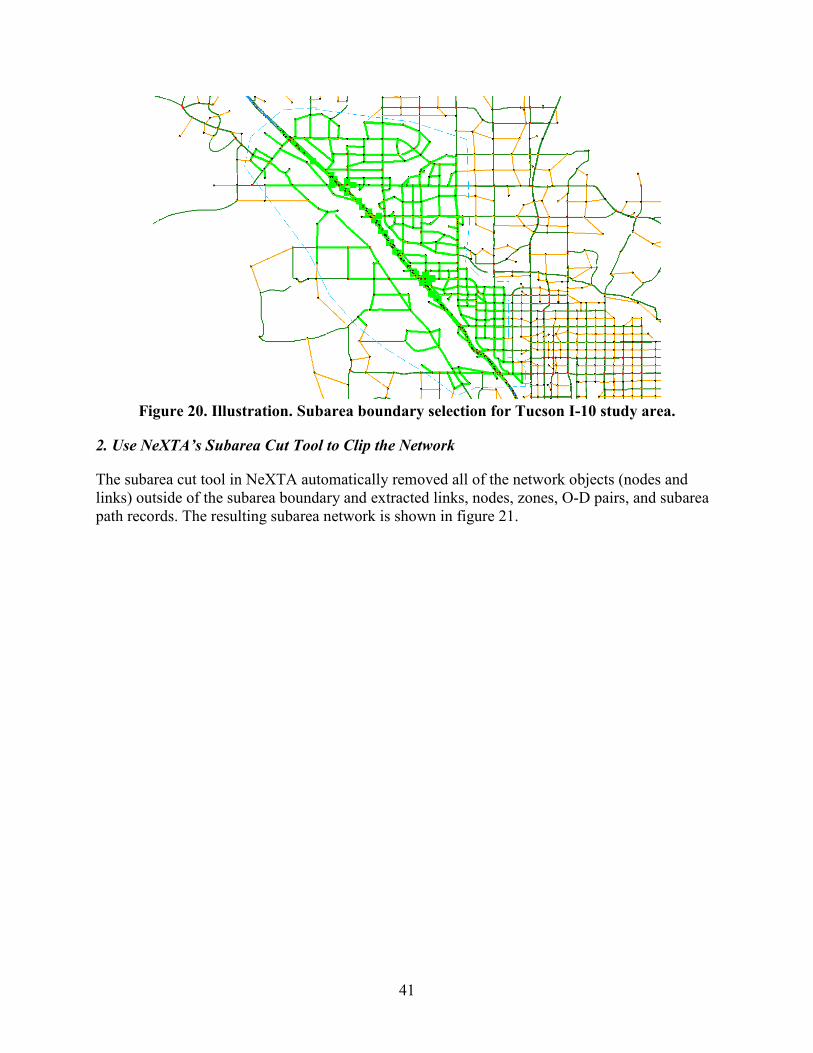
41

Figure 20. Illustration. Subarea boundary selection for Tucson I-10 study area.

2. Use NeXTA’s Subarea Cut Tool to Clip the Network

The subarea cut tool in NeXTA automatically removed all of the network objects (nodes and links) outside of the subarea boundary and extracted links, nodes, zones, O-D pairs, and subarea path records. The resulting subarea network is shown in figure 21.

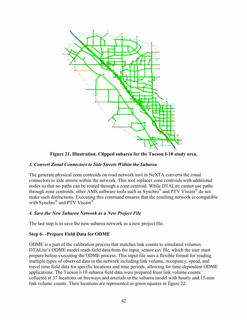
42

Figure 21. Illustration. Clipped subarea for the Tucson I-10 study area.

3. Convert Zonal Connectors to Side Streets Within the Subarea

The generate physical zone centroids on road network tool in NeXTA converts the zonal connectors to side streets within the network. This tool replaces zone centroids with additional nodes so that no paths can be routed through a zone centroid. While DTALite cannot use paths through zone centroids, other AMS software tools such as Synchro® and PTV Vissim® do not make such distinctions. Executing this command ensures that the resulting network is compatible with Synchro® and PTV Vissim®.

4. Save the New Subarea Network as a New Project File

The last step is to save the new subarea network as a new project file.

Step 6—Prepare Field Data for ODME

ODME is a part of the calibration process that matches link counts to simulated volumes. DTALite’s ODME model reads field data from the input_sensor.csv file, which the user must prepare before executing the ODME process. This input file uses a flexible format for reading multiple types of observed data in the network including link volume, occupancy, speed, and travel time field data for specific locations and time periods, allowing for time-dependent ODME applications. The Tucson I-10 subarea field data were prepared from link volume counts collected at 37 locations on freeways and arterials in the subarea model with hourly and 15-min link volume counts. Their locations are represented as green squares in figure 22.

43

Figure 22. Illustration. Subarea field data sensor locations for ODME in DTALite.

Step 7—Run ODME Using Field Data for Calibration

To enable ODME mode in DTALite, the user must set up the input_scenario_settings.csv file and the ODME_Settings.txt file. These files specify the number of iterations, the amount of adjustment allowed per iteration, the calibration time period which can be a portion of the simulation period, and weight on historical O-Ds.

The plots in figure 23 and figure 24 compare the observed and simulated link volumes/counts at the subarea sensor locations. The initial equilibrium assignment (before ODME) produced link volumes that were relatively similar to the observed link volumes with R2 = 0.74, although under- and over-estimation was observed at multiple locations. After running ODME for 10 iterations, the under- and over-estimation was significantly reduced, and the R2 value improved to 0.89 over all observations.

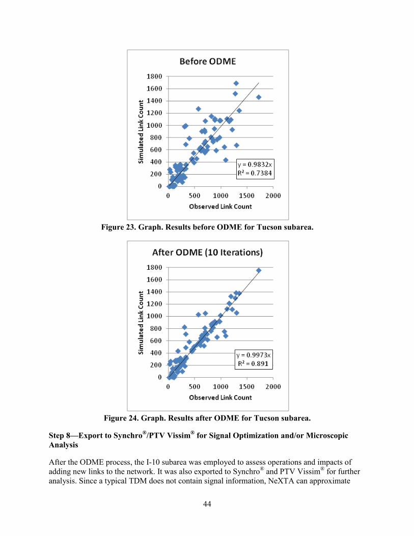
44

Figure 23. Graph. Results before ODME for Tucson subarea.

Figure 24. Graph. Results after ODME for Tucson subarea.

Step 8—Export to Synchro®/PTV Vissim® for Signal Optimization and/or Microscopic Analysis

After the ODME process, the I-10 subarea was employed to assess operations and impacts of adding new links to the network. It was also exported to Synchro® and PTV Vissim® for further analysis. Since a typical TDM does not contain signal information, NeXTA can approximate

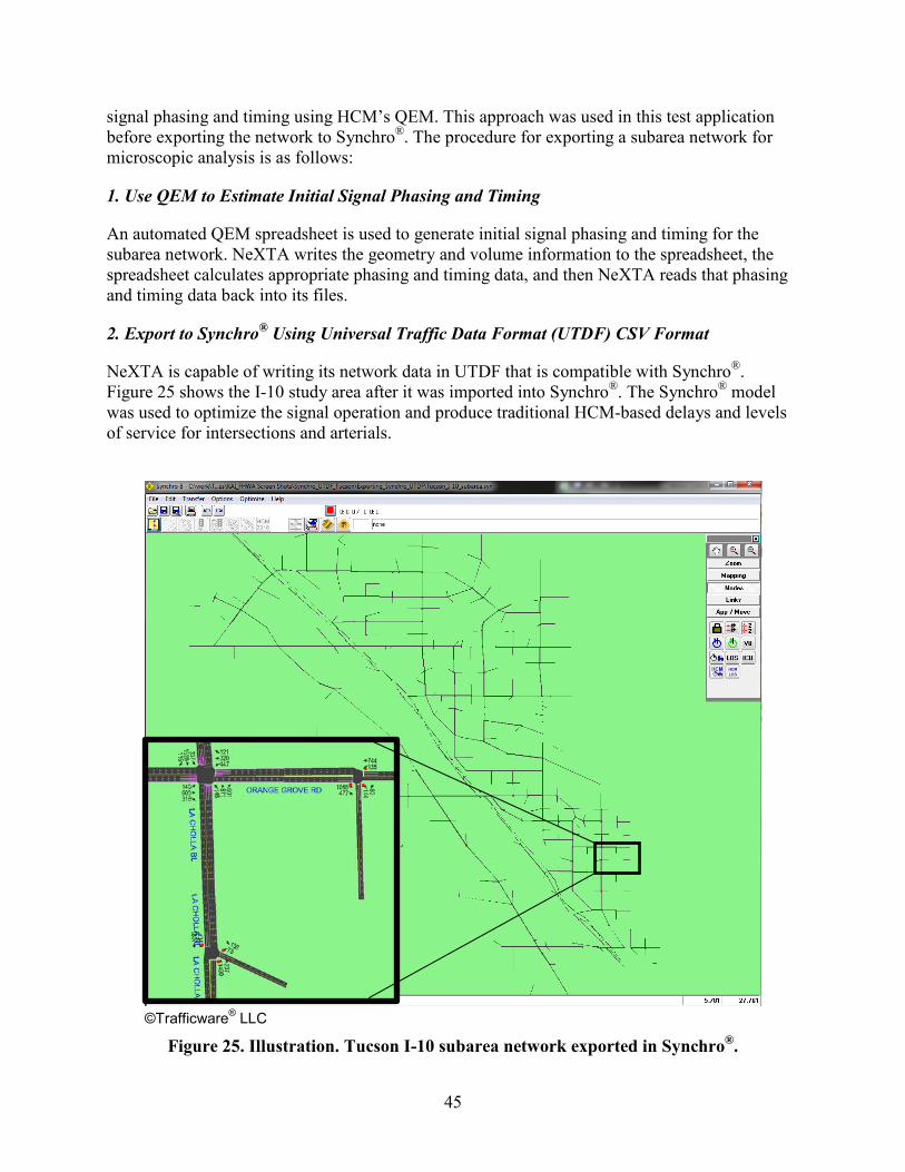
45

signal phasing and timing using HCM’s QEM. This approach was used in this test application before exporting the network to Synchro®. The procedure for exporting a subarea network for microscopic analysis is as follows:

1. Use QEM to Estimate Initial Signal Phasing and Timing

An automated QEM spreadsheet is used to generate initial signal phasing and timing for the subarea network. NeXTA writes the geometry and volume information to the spreadsheet, the spreadsheet calculates appropriate phasing and timing data, and then NeXTA reads that phasing and timing data back into its files.

2. Export to Synchro® Using Universal Traffic Data Format (UTDF) CSV Format

NeXTA is capable of writing its network data in UTDF that is compatible with Synchro®. Figure 25 shows the I-10 study area after it was imported into Synchro®. The Synchro® model was used to optimize the signal operation and produce traditional HCM-based delays and levels of service for intersections and arterials.

©Trafficware® LLC

Figure 25. Illustration. Tucson I-10 subarea network exported in Synchro®.

46

3. Export to PTV Vissim® Using Animation (ANM) Format

The I-10 study area was also exported into PTV Vissim® via the ANM format. ANM is a text-based format developed by PTV Group® to allow the linkage between PTV Vissim ® and other software. NeXTA is capable of generating the .anm and .anmroute files that allow PTV Vissim® to replicate the NeXTA network and vehicle path flows. The imported network in PTV Vissim® is shown in figure 26.

©PTV Group®

Figure 26. Illustration. Tucson I-10 subarea network in PTV Vissim®.

47

SUMMARY

The Tucson test application demonstrated the integration of TDM, DTA, and Synchro®/ PTV Vissim® as well as the successful application of NeXTA to a real-world project. Some of the positive features of the AMS data hub that were noted during the test application include the following:

• Streamlining conversion from a regional TDM to a DTA model: During the conversion, NeXTA intelligently predicted signal locations and assigned default signal parameters to these locations for the entire network. This automation function was a significant time saver since the signal information was not available in the Tucson regional demand model and needed to improve accuracy of the DTA network.

• Automating the creation of subarea: Once the subarea boundary was defined for the I-10 corridor, NeXTA created all the necessary files for the subarea to function as an independent network. Preparation of the O-D matrix for the subarea would have been tedious, if not impossible, if it had been done manually.

• Automating the calibration of a DTA model via ODME: Once segment traffic counts were entered into the sensor input file, NeXTA/DTALite were used to compare simulated volumes against field counts after each iteration and automatically adjusted vehicle paths and the O-D matrix. Other DTA packages would have required several steps and user intervention to achieve desirable results.

• Exporting a network to Synchro® and PTV Vissim®: NeXTA successfully converted the I-10 subarea network into a Synchro® network and PTV Vissim® network. Many agencies still insist on the traditional HCM capacity analyses and level of service results. The linkage to Synchro® (and similar HCM-based software) is beneficial to satisfy this requirement in a cost effective manner.

• Providing a comprehensive list of MOEs and visualization functions: NeXTA was used to visualize multiple MOEs, including time-dependent volume, speed, density, and queuing for individual links. NeXTA also offers the ability to analyze path/corridor travel time and examine subarea/network level statistics for multiple MOEs using vehicle trajectory data produced by the DTA model. Additional visualizations were produced using NeXTA’s export functions to Google Fusion Tables®, with an example shown in figure 27. Figure 27 visualizes both link volume and V/C ratio, where line widths increase with increasing volume and the line color varies by the V/C ratio (red = high and green = low).

48

©2013 Google Maps®

Figure 27. Illustration. Tucson network MOE visualization.(9)

In summary, the AMS data hub achieved its primary goals of creating significant time savings by producing automatic linkages across models through the use of an open source data management tool (NeXTA). The NeXTA prototype overcomes many of the challenges associated with integrated modeling applications; however, the current prototype requires familiarity with the data schema and the ability to set up initial linkages between models. This can be overcome through training and through the development of a more robust relational or object-oriented database system.

49

PORTLAND, OR, TEST APPLICATION RESULTS

INTRODUCTION

This section describes the test application on a step-by-step basis to demonstrate the use of the AMS data hub through NeXTA for a multi-resolution arterial analysis along the NW 185th Avenue corridor and surrounding subarea. Starting with an existing regional TDM, PTV Visum® was imported to the data hub in NeXTA for network and demand adjustments, and an assignment was performed using DTALite. The model was then exported to Synchro® for signal timing modifications and deterministic analysis and then brought back through the AMS data hub into PTV Vissim® for microsimulation analysis. Because of the congested nature of this geographic area, the application examined a time period from 2 p.m. to 7 p.m.

The steps for this Portland arterial application are summarized in this section.

Step 1—Export Network from Regional TDM

Portland Metro maintains the Portland regional TDM in PTV Visum®. This network was converted to a set of shape files before importing it into NeXTA. This was accomplished using the shape file export function in PTV Visum®. It is recommended to import the full regional TDM (assigned or unassigned) into the AMS data hub through NeXTA to retain accuracy. This network export is accomplished using the following steps:

1. Load the Network in PTV Visum® and Export the Network as Shape Files

First, the network was loaded in PTV Visum® as shown in Figure 28 .

50

©PTV Group®

Figure 28. Illustration. Portland regional TDM loaded in PTV Visum®.

By using the function in PTV Visum® to export the network GIS shape files, the network is split into components and saved as multiple separate shape files. Users should select the node, link, zone, zone centroid, and connector layers to ensure that the conversion process can successfully create a new network in the AMS data hub. Exporting to shape files in PTV Visum® requires the GIS interface shape add-on module. An example of PTV Visum® shape file export options is shown in Figure 29.

51

©PTV Group®

Figure 29. Screenshot. Shape file export options in PTV Visum®.

Intermediate Step—Change Map Projection to WGS84

PTV Visum® exports the shape files in the network’s current coordinate or map projection system. To simplify the conversion process, it is recommended to change from the NAD83 system to the WGS84 system before being imported into NeXTA. This process was completed using projection tools in the ESRI® ArcGIS software.

2. Export Demand Tables/Matrices

The zone matrices in PTV Visum® are compatible with the demand definition in NeXTA. Users should save the matrix files from PTV Visum® into the “Format O” option when preparing tables for export to NeXTA. Exporting the demand matrices for the Portland TDM produces 20 demand tables describing the number of trips between zones for different demand types (single-occupant vehicle (SOV), high-occupancy vehicle (HOV), heavy trucks, and medium trucks) for the time period between 2 p.m. and 7 p.m., as shown in Figure 30 and Figure 31.

52

©PTV Group®

Figure 30. Screenshot. Saving demand matrices in PTV Visum® to be imported into NeXTA.

©PTV Group®

Figure 31. Screenshot. Matrix export options in PTV Visum®.

Step 2—Import Network from Regional TDM

The second step in the AMS data hub network conversion process is to use NeXTA’s network import tool to convert the network shape files into the AMS data hub format. This process reads the spatial data stored in each specified shape file, along with the corresponding data stored in the database file (DBF) to create the input CSV files used by the AMS data hub in NeXTA. In

53

order to interpret the DBFs for conversion, an INI file is used to map field names between the shape files and the standard data format used in NeXTA.

The network import process is divided into the following three internal steps:

1. Prepare INI Configuration File and Attribute Files for Conversion

The first step in converting the network is to create an INI configuration file in the folder containing the exported shape files. NeXTA uses this user-defined configuration file to associate/map fields in shape file DBF files to the AMS data hub schema data format, allowing NeXTA to read the network geometry from shape files and create an AMS data hub compatible .tnp file.

The configuration file is divided into different sections depending on the type of data to be imported. The first section describes general model attributes and import options. The remaining sections are used to describe the different types of network objects that can be imported. Separate sections are used to import links and nodes, with optional sections for importing zones, zone centroids, and zonal connectors. Once a configuration file is established for a regional travel demand format, it can be replicated for future imports from that format. Since the Portland PTV Visum® model has the intersection control type defined, this is brought into the AMS data hub in NeXTA through this conversion file.

2. Use NeXTA’s Import Network Tool to Convert the Network

Next, the regional TDM (network, demand, control, etc.) was imported into NeXTA through the INI configuration file created to link the shape files to the NeXTA format (see figure 32 and figure 33).

Figure 32. Screenshot. Network import menu location in NeXTA.

54

Figure 33. Screenshot. Import configuration INI file in NeXTA.

After the successful conversion process, NeXTA displays a “File Loading Status” window as shown in figure 34.

Figure 34. Screenshot. File loading status window displaying import results.

The final imported Portland network is shown in figure 35, which has 2,162 zones, 39,770 links, and 14,721 nodes. It should be noted that control type (signal, stop, and yield) is imported from the Portland PTV Visum® network into NeXTA.

55

Figure 35. Illustration. Portland regional network imported into NeXTA/DTALite.

3. Save the New Network as a New Project File

The network was saved as a new .tnp file, which is the native file type for NeXTA.

Step 3—Read Demand Data from Regional TDM

Similar to the INI file, the input_demand_meta_data.csv file is used by NeXTA to find and read the O-D/trip tables (matrix (MTX) files from PTV Visum®) exported from the TDM. This metadata file requires several entries. The relevant entries include the following:

1. Specify the demand file name (e.g., sov_14_15.mtx) and format (e.g., column).

2. Specify the number of lines in the demand file to be skipped by NeXTA (eight for MTX file).

3. Indicate whether subtotals are present in the last column (zero for none).

4. Specify the loading start time and end time for the demand file (e.g., 840 to 900 or 2 p.m. to 3 p.m.).

5. Specify the demand types associated with the demand file (only demand_type1).

56

Step 4—Run Assignment with DTALite to Equilibrium

Before a subarea is created for more detailed analyses, DTA is recommended to ensure equilibrium network path flows and thus reasonable trips entering the subarea.

DTA was performed with a DTALite assignment engine (directly accessed in NeXTA). Simulation settings should be edited in the input_scenario_settings.csv file prior to initiating the assignment engine (e.g., selecting simulation from one of the NeXTA toolbars).

DTALite is fairly efficient. For the Portland regional network with 15 simulation runs for about 1,100,000 vehicles, DTALite took 1 h13 min to complete on an Intel® Core I7 2760QM (2.4–3.5 GHz quad core) with 32 GB RAM. This resulted in an average travel time of 26.18 min and an average trip length of 7.72 mi.

Step 5—Cut a Subarea within the Larger Model for More Detailed Analysis

For the 185th Avenue arterial network, a smaller focused subarea was defined by the highway interchange at the north and the light rail crossing to the south, encompassing 16 signalized intersections. NeXTA greatly simplifies the subarea creation process by automatically extracting necessary nodes, links, zones, and O-D tables when creating a subarea.

The subarea creation process is divided into the following four internal steps:

1. Create a Subarea Boundary in NeXTA

A subarea boundary was drawn around the NW 185th Avenue evaluation area used for this test case using the create subarea tool in NeXTA. After drawing the boundary, the links and nodes within the boundary were highlighted by NeXTA, as shown in figure 36. The highlight allows a visual assessment of the boundary, and adjustments can be made if needed.

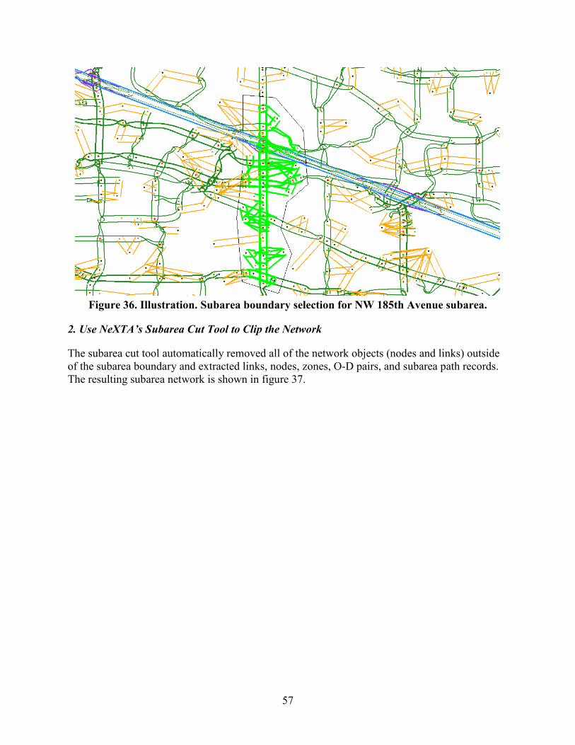
57

Figure 36. Illustration. Subarea boundary selection for NW 185th Avenue subarea.

2. Use NeXTA’s Subarea Cut Tool to Clip the Network

The subarea cut tool automatically removed all of the network objects (nodes and links) outside of the subarea boundary and extracted links, nodes, zones, O-D pairs, and subarea path records. The resulting subarea network is shown in figure 37.

58

Figure 37. Illustration. Clipped subarea for the NW 185th Avenue subarea.

3. Convert Zonal Connectors to Side Streets Within the Subarea

This tool converts the zonal connectors to side streets within the network. It replaces zone centroids with additional nodes so that no paths can be routed through a zone centroid. While DTALite cannot use paths through zone centroids, other analysis software such as Synchro® and PTV Vissim® does not make such distinctions. Executing this command ensures that the resulting network is compatible with Synchro® and PTV Vissim®. The resulting network created by using this tool is shown in figure 38.

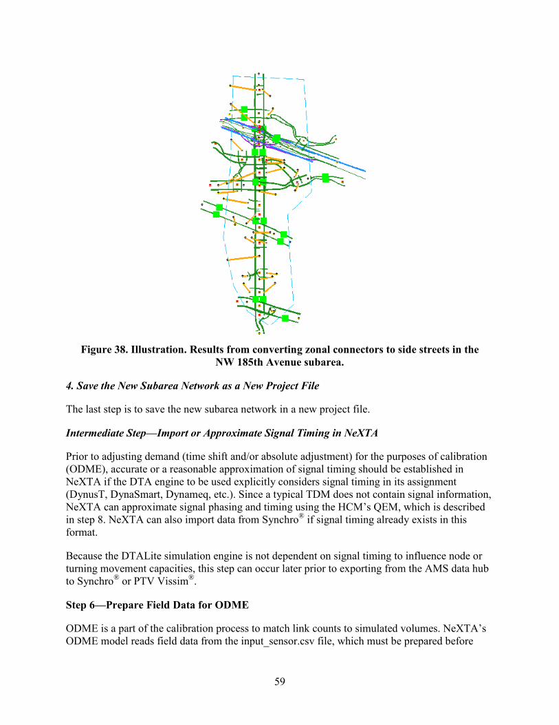
59

Figure 38. Illustration. Results from converting zonal connectors to side streets in the

NW 185th Avenue subarea.

4. Save the New Subarea Network as a New Project File

The last step is to save the new subarea network in a new project file.

Intermediate Step—Import or Approximate Signal Timing in NeXTA

Prior to adjusting demand (time shift and/or absolute adjustment) for the purposes of calibration (ODME), accurate or a reasonable approximation of signal timing should be established in NeXTA if the DTA engine to be used explicitly considers signal timing in its assignment (DynusT, DynaSmart, Dynameq, etc.). Since a typical TDM does not contain signal information, NeXTA can approximate signal phasing and timing using the HCM’s QEM, which is described in step 8. NeXTA can also import data from Synchro® if signal timing already exists in this format.

Because the DTALite simulation engine is not dependent on signal timing to influence node or turning movement capacities, this step can occur later prior to exporting from the AMS data hub to Synchro® or PTV Vissim®.

Step 6—Prepare Field Data for ODME

ODME is a part of the calibration process to match link counts to simulated volumes. NeXTA’s ODME model reads field data from the input_sensor.csv file, which must be prepared before

60

executing the ODME process. This input file uses a flexible format for reading multiple types of observed data in the network, including link volume, occupancy, speed, and travel time field data for specific locations and time periods, allowing for time-dependent ODME applications.

The NW 185th Avenue subarea field data were prepared from link volume counts collected at 21 locations on freeways and arterials in the subarea model, with hourly and 15-min link volume counts. Their locations are represented as green squares in figure 39.

Figure 39. Illustration. Subarea field data sensor locations for ODME in NeXTA.

Step 7—Run ODME Using Field Data for Calibration

To enable the ODME mode in NeXTA, the input_scenario_settings.csv file and the ODME_Settings.txt file must be set up. These files specify the number of iterations, the amount of adjustment allowed per iteration, the calibration time period that can be a portion of the simulation period, and weight on historical O-Ds.

For this example, the assignment engine was specified to run for five iterations to arrive at a relatively stable operating condition. The ODME module was then used to adjust path flows over the following 75 iterations. The ODME module in DTALite was set to adjust 5 percent of the O-D demand after each iteration, allowing the model to run to completion faster without sacrificing solution quality. Time-dependent link volume/count data were used for calibration, allowing for more detailed O-D flow refinements.

Two plots shown in figure 40 and figure 41 compare the observed and simulated link volumes/counts at the subarea sensor locations. The initial equilibrium assignment (before ODME) produced link volumes that were relatively similar to the observed link volumes with

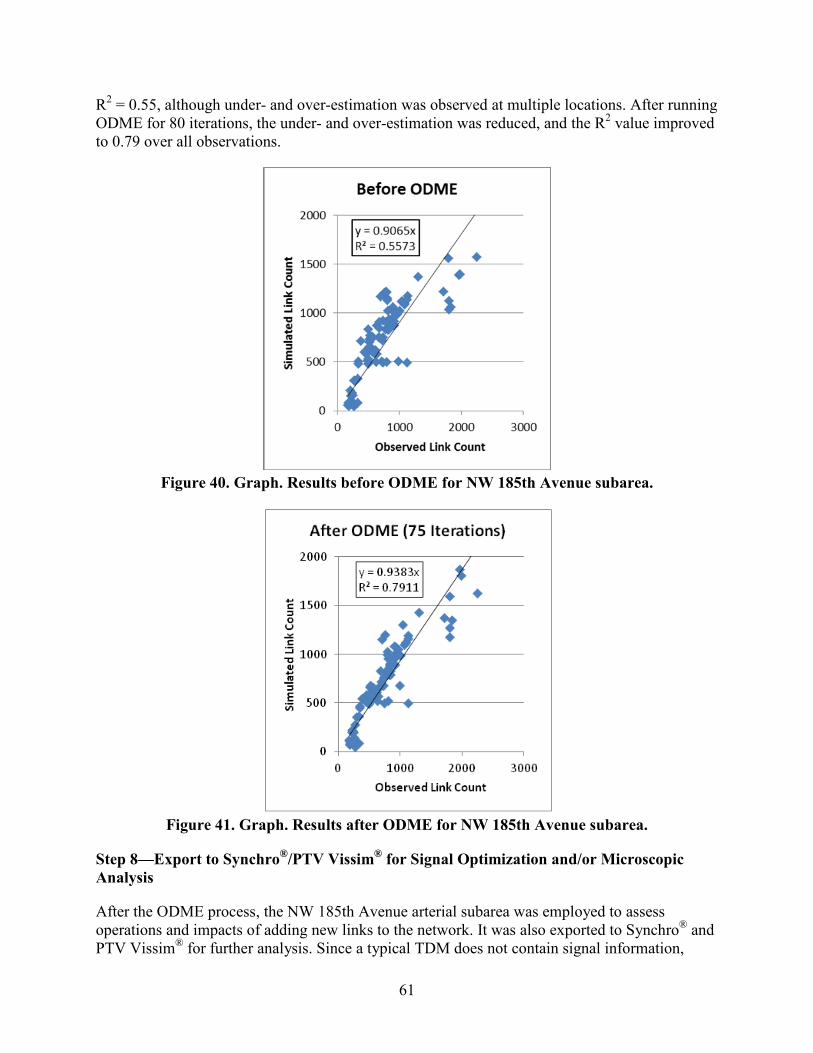
61

R2 = 0.55, although under- and over-estimation was observed at multiple locations. After running ODME for 80 iterations, the under- and over-estimation was reduced, and the R2 value improved to 0.79 over all observations.

Figure 40. Graph. Results before ODME for NW 185th Avenue subarea.

Figure 41. Graph. Results after ODME for NW 185th Avenue subarea.

Step 8—Export to Synchro®/PTV Vissim® for Signal Optimization and/or Microscopic Analysis

After the ODME process, the NW 185th Avenue arterial subarea was employed to assess operations and impacts of adding new links to the network. It was also exported to Synchro® and PTV Vissim® for further analysis. Since a typical TDM does not contain signal information,

62

NeXTA can approximate signal phasing and timing using HCM’s QEM. This approach was used in this test application before exporting the network to Synchro®. The procedure for exporting a subarea network for microscopic analysis is divided into the following three steps:

1. Use QEM to Estimate Initial Signal Phasing and Timing

An automated QEM spreadsheet is used to generate initial signal phasing and timings for the subarea network. NeXTA writes the geometry and volume information to the spreadsheet, the spreadsheet calculates appropriate phasing and timing data, and then NeXTA reads that phasing and timing data back into its files.

2. Export to Synchro® Using UTDF CSV Format

NeXTA is capable of writing its network data in the UTDF format that is compatible with Synchro®. The NW 185th Avenue study area is shown in Figure 42 after being imported into Synchro®. The Synchro® model was used to optimize the signal operation and produce traditional HCM-based delays and levels of service for intersections and arterials.

©Trafficware® LLC

63

Figure 42. Screenshot. NW 185th Avenue subarea network imported into Synchro®.

3. Export to PTV Vissim® Using ANM Format

The NW 185th Avenue study area was also exported into PTV Vissim® via the ANM format. The imported network in PTV Vissim® is shown in Figure 43.

©PTV Group®

Figure 43. Illustration. NW 185th Avenue subarea network imported in PTV Vissim®.

SUMMARY

The Portland test application successfully demonstrated the seamless transfer between common AMS tools to facilitate from an established regional TDM to DTALite for mesoscopic analysis, Synchro® for deterministic and signal timing analysis, and PTV Vissim® for microscopic analysis.

The AMS data hub enables a host of time saving analysis features relative to the arterial multi-modal network. The following are key features highlighted as benefits of the AMS data hub:

• Import signal timing files from Synchro® or automatically create signal timing parameters via QEM as a reasonable starting point for intersection capacity for DTA, deterministic, and microsimulation analyses.

• Quickly import existing TDM into multiple DTA platforms (e.g., DTALite and DynusT).

• Embedded tools and functionality in NeXTA to support the multi-resolution process through the AMS data hub including the following:

64

o Visualization tools to quickly and easily compare link counts to simulated volumes (R2 correlation).

o CSV format to allow easy user modification of settings and data sources.

o Easy demand adjustment tools to shift by time of day factoring or a full O-D matrix adjustment in ODME. This is particularly useful in model calibration, which can take the majority of time in AMS tools. This represents the potential for very large time savings.

o MOEs and other visualizations in NeXTA to observe DTA level results (i.e., V/C ratio, queuing, travel time, reliability, etc.) in a time-dependent setting, which supports a new generation of performance measurements for system management (i.e., hours of congestion, travel time reliability, etc.).

• Export functionality to Google Maps® and Google Earth® allows for easy sharing of results in a common visualization package.

Much like the Tucson, AZ, application, this effort did not concentrate on generating actual results from the converted model. Instead, it focused on the functioning links created through the AMS data hub.

This Portland test application achieved its primary goal to demonstrate the usefulness of the AMS tool in solving real-world problems. NeXTA has overcome many issues to reach this level of integration; however, one challenge a typical user faces is becoming familiar with the NeXTA file format that comprises of many CSV files and entry fields and being able to set up CSV files manually. This can be overcome through training and through developing a more robust relational or object-oriented database system.

Beneficial NeXTA features noted during the test application include the following:

• Streamlining the conversion from a regional TDM to a DTA model: During the conversion, NeXTA predicted signal locations and assigned default signal parameters to these locations for the entire network. This automation function was a huge time saver since the signal information was not available in the Tucson regional demand model and needed to improve accuracy of the DTA network.

• Automating the creation of subarea: Once the subarea boundary was defined for the NW 185th Avenue corridor, NeXTA created all the necessary files for the subarea to function as an independent network. Preparation of the O-D matrix for the subarea would have been tedious, if not impossible, if it have been done manually.

• Automating the calibration of a DTA model via ODME: Once segment traffic counts were entered into the sensor input file, NeXTA/DTALite compared simulated volumes against field counts after each iteration and automatically adjusted vehicle paths and the O-D matrix. Other DTA packages would have required several steps and user intervention to achieve desirable results.

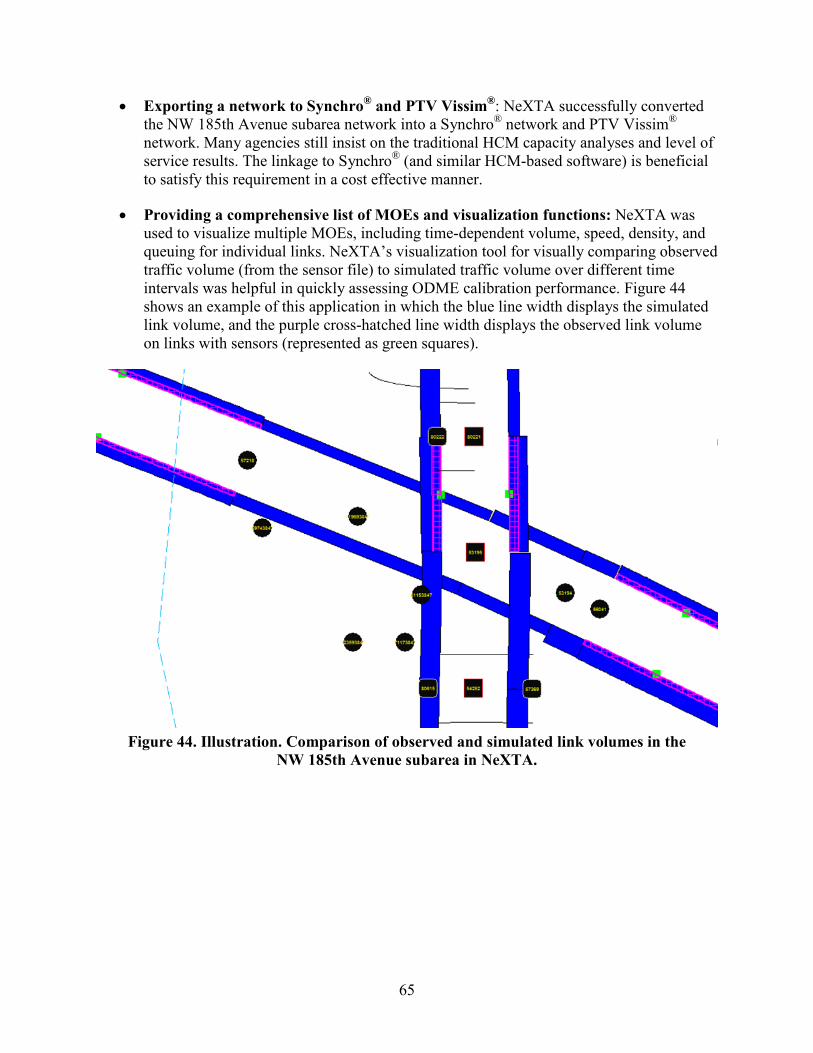
65

• Exporting a network to Synchro® and PTV Vissim®: NeXTA successfully converted the NW 185th Avenue subarea network into a Synchro® network and PTV Vissim® network. Many agencies still insist on the traditional HCM capacity analyses and level of service results. The linkage to Synchro® (and similar HCM-based software) is beneficial to satisfy this requirement in a cost effective manner.

• Providing a comprehensive list of MOEs and visualization functions: NeXTA was used to visualize multiple MOEs, including time-dependent volume, speed, density, and queuing for individual links. NeXTA’s visualization tool for visually comparing observed traffic volume (from the sensor file) to simulated traffic volume over different time intervals was helpful in quickly assessing ODME calibration performance. Figure 44 shows an example of this application in which the blue line width displays the simulated link volume, and the purple cross-hatched line width displays the observed link volume on links with sensors (represented as green squares).

Figure 44. Illustration. Comparison of observed and simulated link volumes in the

NW 185th Avenue subarea in NeXTA.

67

CONCLUSIONS AND RECOMMENDATIONS

The objective of this project was to develop a concept of operations to enable harmonious information exchange and data transferability among models of various domains and scales and to demonstrate the application of new methods and tools through a proof of concept and prototype demonstration.

The AMS data hub concept identifies a system of components necessary for effective model integration including a data schema, network editing tools, data conversion utilities, calibration utilities, and visualization tools. It also includes a cloud-based component to enable collaboration across multiple users and further visualization capabilities.

Test applications were successfully completed for test networks in Portland, OR, and Tucson, AZ. Demonstrations were performed for the respective modeling agencies (Portland Metro and PAG) and were well received. Both agencies are interested in further developing the AMS data hub concept to enable better linkages with signal timing data and DTA packages as well as conducting pilot tests using the AMS data hub tools.

The test applications achieved a time savings of 80 percent. The applications also demonstrated the ability to expand the use of AMS tools within an integrated modeling application which, in turn, improves the quality of results and results in better informed decisionmaking.

As this project resulted in a prototype and proof of concept, several steps are needed to continue to advance the AMS data hub concept so that it can be applied by many users for widespread integrated modeling applications across the United States and internationally.

Key recommendations for future advancement of the AMS data hub concept are as follows:

• Conduct a Webinar with a group of stakeholders that collectively represent modeling agencies, software developers, and consultant practitioners. The purpose of the Webinar should be to solicit feedback and input on the AMS data hub concept and encourage beta testing using the NeXTA data hub tool.

• Conduct a pilot test using the AMS data hub as part of a real-world modeling application. Portland Metro has expressed interest in applying the AMS data hub tools as part of a subarea planning effort being conducted in Clackamas County, OR.

• Develop a linkage between the AMS data hub and activity-based models. Interest has been expressed in this functionality, particularly from members of the Strategic Highway Research Program 2 C10 project teams. This linkage would enable the use of a DTA program to feed travel times back to the tour-based assignment approach.

• Expand the suite of conversion utilities to provide two-way linkages with an expanded set of AMS tools that are commonly used in practice.

• Provide integration capabilities with real-time detector data.

68

• Continue to test and advance methods for developing and incorporating planning-level signal timing plans into mesoscopic models to improve the accuracy of travel time estimation and assignment on arterial networks. Also, linkages should be developed to import signal-timing data from controllers into the data hub and ultimately convert to the required format for common AMS tools that require signal-timing data.

• Explore the feasibility of establishing a robust relational or object-oriented database for storing and managing data from all resolutions of AMS tools and data sources. This type of system is essential for achieving full interoperability among AMS tools.

69

APPENDIX A. INI CONFIGURATION FILE

The following tables describe the variables contained within the INI configuration file.

Table 9. Model attributes configuration settings. Variable Assignment Description/Explanation

units=MI The original network describes distances in units of miles

direction_field=1 “1” indicates that NeXTA uses a direction field to interpret the link shape file

control_type_field=0 “0” indicates that NeXTA does not read any control type information from the node shape file

reserve_direction_field=1 “1” indicates that NeXTA will read direction-specific information for some non-directed links (two-way links)

offset_link=1 “1” indicates that NeXTA will add space between directional links to aid visualization

link_capacity_flag=0 “0” indicates that the link capacity is described on a per-lane basis

number_of_lanes_for_two_way_links=0 “0” indicates that lanes on two-way links are described using the number of lanes in each direction

use_optional_centroid_layer=0 “0” indicates that there is no additional shape file to read which only contains zone centroids

use_optional_connector_layer=0 “0” indicates that there is no additional shapefile to read which only contains zonal connector links

Table 10. Node import configuration settings.

Variable Assignment Description/Explanation reference_file_name=Node_WGS84_202ft.shp Identifies “Node_WGS84_202ft.shp” as the

shape file that describes the nodes in the network

node_id=ID Identifies “ID” as the name of the field that contains unique node numbers

TAZ=TAZID Identifies “TAZID” as the name of the field that contains zone numbers mapped to the associated node numbers

70

Table 11. Link import configuration settings. Variable Assignment Description/Explanation

reference_file_name=Roadway_WGS84_202ft.shp Identifies “'Roadway_WGS84_202ft.shp” as the shape file that describes the links in the network

from_node_id=FROM_NODE Identifies “FROM_NODE” as the name of the field that describes the starting node number for one direction on a link

to_node_id=TO_NODE Identifies “FROM_NODE” as the name of the field that describes the ending node number for one direction on a link

link_id=ID Identifies “ID” as the name of the field that contains unique link numbers

name=ST_NAME Identifies “ST_NAME” as the name of the field that contains a street name for each link

length_in_mile=LENGTH Identifies “LENGTH” as the name of the field describing the length (in miles) of each link

direction=DIR Identifies “DIR” as the name of the field that describes each link’s directional properties (0 or 2 = two-way, 1 = one-way, -1 = opposite direction from FROM/TO notation)

link_type =FT Identifies “FT” as the name of the field that describes the functional classification (equivalent to link type in NeXTA/DTALite) for the directional link in FROM/TO notation

number_of_lanes=AB_LANES Identifies “AB_LANES” as the name of the field that describes the number of lanes on the directional link in FROM/TO notation

lane_capacity_in_vhc_per_hour AB_CAPACIT Identifies “AB_CAPACIT” as the name of the field that describes the lane capacity on the directional link in FROM/TO notation

speed_limit_in_mph=AB_SPEED1 Identifies “AB_SPEED1” as the name of the field that describes the free-flow speed on the directional link in FROM/TO notation

r_link_type =FT Identifies “FT” as the name of the field that describes the functional classification (equivalent to link type in NeXTA/ DTALite) for the directional link in TO/FROM notation. There was no separate field for functional class in the reverse direction, so the same functional class was

71

used for both directions r_number_of_lanes =BA_LANES Identifies “BA_LANES” as the name of the

field that describes the number of lanes on the directional link in TO/FROM notation

r_lane_capacity_in_vhc_per_hour=BA_CAPACIT Identifies “BA_CAPACIT” as the name of the field that describes the lane capacity on the directional link in TO/FROM notation

r_speed_limit_in_mph=BA_SPEED1 Identifies “BA_SPEED1” as the name of the field that describes the free-flow speed on the directional link in TO/FROM notation

73

APPENDIX B. DATA SCHEMA

This section describes a unified data structure that facilitates input/output data conversion in the short term and promotes data consistency and exchange in the long term.

The component diagram shown in figure 3 illustrates the relationship of the nine tables in the proposed database schema. A few notes regarding the component diagram are as follows:

• The arrow indicates the parent-child relationship. For example, a zone can have one or more links; a link can have nodes, demands, or performance measures; a node can have a signal, stop-control, or roundabout; etc.

• The signals and trajectory tables are currently applicable only to mesoscopic and microscopic resolutions.

• As previously mentioned, HCM-based tools fall between the mesoscopic and microscopic categories. As such, some table data are applicable to the HCM-based tools.

• The configuration table is independent of the other tables.

Advantages of the database schema are as follows:

• It is software neutral, meaning it can be applied using any software program.

• The database tables that are initially proposed can be expanded in the future.

• Software can be configured to read all or a subset of parameters in a table.

• A software vendor can add field parameters that are specific to its product.

• Links and nodes are geo-coded and thus are more easily integrate with GIS and other visualizers such as Google Maps®.

• Since the data structure is transparently and openly defined, it can be readily scrutinized, tested, and enhanced.

• The database schema can serve as a platform to encourage the development of analysis tools and visualization tools, especially from small software vendors and researchers.

• The database schema moves the practice of integrated modeling towards a standard for how modeling data should be stored and shared.

One major disadvantage of such an overarching, unified data schema is its size, which has an adverse effect on computation speed and efficiency. The data structure is understandably large in order to accommodate analysis models in various resolutions. As such, a single intersection analysis using the HCM method would utilize only a small portion of the data structure.

74

A description for each of the components of the database schema is provided in the following subsections. The descriptions are general in nature, but the database schema can be implemented in XML or a database format.

DATABASE SYSTEM

The data hub will need to be able to handle a wide variety of data types, some of which are complex. Examples of simple and complex data types include the following:

Simple Data Types:

• Strings: Alphanumeric fields that are typically short (less than 200 characters) and contain descriptive or type data.

• Integers: Used for floating point numbers.

Complex Data Types:

• Coordinates: Used to specify geographic locations of points such as nodes. A series of coordinates is used to define a shape such as a link or a zone boundary. Coordinates are specified in a predefined system (e.g., latitude/longitude or UTM).

• Geometry: Needed to specify boundaries, in the case of zones, or paths, in the case of links.

In the proposed database schema, the data type definitions listed in table 6.

ZONES

Existing Practice

In the existing practice, zones are used in TDM and DTA. TDMs include TAZs that typically list the number of automobiles per household, household income, and employment. DTA models also adopt the TAZs from TDMs. In addition, DTA models like DynusT introduce super zones, which comprise of one or more zones for evacuation evaluation. Synchro® also uses the zone concept to divide a network into zones to facilitate signal optimization or output for a portion of the network. Microsimulation software, most HCM-based tools, and field data do not use the zone concept.

Challenges

Generally, there are no obvious challenges to define zones for all resolutions. However, a few minor definition issues include the following:

• A link can be dissected by a zone boundary and as a result is physically located in more than one zone. One solution is to include Link_a in Zone_i if more than 50 percent of the link length is located within Zone_i. In rare cases where a link is evenly split between two zones, the link can be assigned to the zone with fewer links or smaller ID.

75

• When zones are manually defined by an analyst, it is possible that there are portions of a network that do not belong to any zone. A function should be included in the user interface (such as NeXTA) to check for and correct these gaps.

Proposed Structure

The data structure proposed for zones (see table 12) meets current AMS needs and provides the flexibility to expand in the future. In this structure, a zone can have many nodes and links. Specifically, a zone is the “parent” of nodes and links. For consistency, it is suggested that a zone is initially defined in accordance with TAZs and that a super zone or jurisdiction is a collection of zones.

Table 12. Proposed zones data structure. Field Description Type Notes

Zone ID Zone identification number

Numerical None

Zone name Zone name Alphanumeric None Boundary Geo-coded boundary Geometric <coordinate> (x1, y1)

(x2, y2) (x3, y3) ...</coordinate>

Super zone ID of the super zone that the zone belongs

Numerical None

Jurisdiction Jurisdictional code and/or name that the zone belongs

Alphanumeric #-Jurisdiction_name

The subarea cut table is a subset of the zones table. Each subarea table contains data and information about a smaller study area or a corridor as well as links to other tables that allow detailed analyses to be conducted. Subset table with sample fields for a subarea is illustrated in table 13.

76

Table 13. Subarea zone table with sample subarea fields. Field Description Value Notes

Subarea ID Subarea or path identification number

Numerical None

Zone ID Zone identification number

Numerical None

Zone name Zone name Alphanumeric None Boundary Geo-coded boundary Alphanumeric <coordinate> (x1, y1)

(x2, y2) (x3, y3) ...</coordinate>

Node ID IDs of all nodes within zone i

Numerical Nodea, Nodeb, Nodec...

Link ID IDs of all links within zone i

Numerical Link_a, Link_b, Link_c, Link_d...

The zone socioeconomic table maintains socioeconomic data for each TAZ. These data will change with each scenario. Table 14 shows some types of data that would go into a socioeconomic table. Note that different planning agencies have their own definitions of socioeconomic variables that are used for travel forecasting. Examples are as follows:

• Households can be divided into the following different groups:

o Dwelling unit types (e.g., single family, multi-family, etc.).

o Income categories (e.g., income quartiles).

o Age of head.

o Auto ownership category.

• Employment is often divided into different categories (e.g., manufacturing, service, retail, etc.).

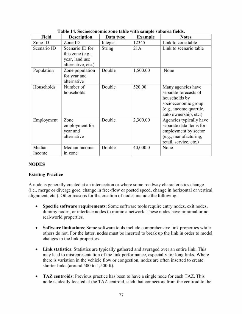
77

Table 14. Socioeconomic zone table with sample subarea fields. Field Description Data type Example Notes

Zone ID Zone ID Integer 12345 Link to zone table Scenario ID Scenario ID for

this zone (e.g., year, land use alternative, etc.)

String 21A Link to scenario table

Population Zone population for year and alternative

Double 1,500.00 None

Households Number of households

Double 520.00 Many agencies have separate forecasts of households by socioeconomic group (e.g., income quartile, auto ownership, etc.)

Employment Zone employment for year and alternative

Double 2,300.00 Agencies typically have separate data items for employment by sector (e.g., manufacturing, retail, service, etc.)

Median Income

Median income in zone

Double 40,000.0 None

NODES

Existing Practice

A node is generally created at an intersection or where some roadway characteristics change (i.e., merge or diverge gore, change in free-flow or posted speed, change in horizontal or vertical alignment, etc.). Other reasons for the creation of nodes include the following:

• Specific software requirements: Some software tools require entry nodes, exit nodes, dummy nodes, or interface nodes to mimic a network. These nodes have minimal or no real-world properties.

• Software limitations: Some software tools include comprehensive link properties while others do not. For the latter, nodes must be inserted to break up the link in order to model changes in the link properties.

• Link statistics: Statistics are typically gathered and averaged over an entire link. This may lead to misrepresentation of the link performance, especially for long links. Where there is variation in the vehicle flow or congestion, nodes are often inserted to create shorter links (around 500 to 1,500 ft).

• TAZ centroids: Previous practice has been to have a single node for each TAZ. This node is ideally located at the TAZ centroid, such that connectors from the centroid to the

78

road network are representative of average travel times from the TAZ to the rest of the transportation network. The newer activity-based models often require much finer-grained representation of connections of different TAZ subareas (or even individual land parcels) to the transportation network. Hence, the trend is to have multiple nodes to represent different subareas within each TAZ.

It should be noted that some software tools create nodes automatically and store them internally when links are created. Some tools define nodes as locations where statistics need to be collected, and they have no physical attributes.

Challenges

Some challenges when integrating different datasets include the following:

• Some software tools have limitations on the number of nodes and numbering scheme.

• Some software tools do not use nodes explicitly. PTV Vissim® uses connectors to store properties that may often be associated with nodes.

• Some software tools generate nodes automatically.

Proposed Structure

Similar to the link table, the data structure proposed for nodes aims to replicate the physical real-world conditions as much as possible. The goal is to rely on software developers or conversion modules to aggregate the data into a format usable by specific software. Some suggestive guidelines for node creation and placement include the following:

• More than one node may be required to adequately represent connections between different subareas of the TAZ to the transportation network.

• Nodes should be used to represent signalized intersections, roundabouts, stop-control intersections, yield control intersections, major driveways, and merge/diverge areas.

• Intermediate nodes should be used to limit link length to 1,500 ft.

• For freeway merge and diverge locations, nodes should be placed where edge stripes meet.

• For intersections, nodes should be placed at the middle of the intersections. Node properties such as stop bar locations can be employed to delineate the intersections’ dimensions.

• Node locations should be geo-coded so that they can be displayed in Google Maps®/Google Earth® or synchronized with various GIS layers.

79

A normalized table structure for nodes is recommended as follows:

• Geographic features that will not change (i.e., node location) are kept in one table.

• Geometric features may change with different scenarios. For example, for some nodes, left turns may not be permitted during peak hours.

• Traffic volumes will change with scenarios and are therefore represented in a separate table.

Sample fields in the node tables include the following:

• Table 15 shows the base node table. The table is limited to defining the node location, node type, and the TAZ that contains the node.

• Table 16 shows the node geometry table. There is one record per approach for each node. Because node geometry may change with scenarios, separate records are required for each scenario.

• Table 17 shows the table for node volumes. There is one record per approach for each node.

The node volumes, node geometry, and signal phasing tables are used to develop MOEs.

Table 15. Sample fields in the base node table. Field Description Data Type Example

Node Node number or ID Integer 1234 Longitude Longitude Double 37.77138056 Latitude Latitude Double -122.4386917 Node type Facility type of node

(e.g., freeway, arterial, ramp, rail line, bus line, etc.)

Enumeration Rail station

Zone ID of containing TAZ Integer 221

80

Table 16. Sample fields in the node geometry table. Field Description Data Type Example

Scenario Scenario ID String 21A Node Node number or ID Integer 1234 Approach direction Direction of approach

traffic (e.g., N would indicate northbound traffic)

Enumeration N

Lanes—left Number of left turn lanes

Integer 1

Lanes—left thru Number of shared through left-turn lanes

Integer 1

Lanes—left thru right Number of shared left-through-right lanes

Integer 1

Lanes—thru Number of through lanes

Integer 2

Lanes—thru right Number of shared through right-turn lanes

Integer 1

Lanes—right Number of right-turn lanes

Integer 0

Permitted Right Turn on Red

Right turn on red permitted

Boolean F (false)

Free right Free right turn permitted

Boolean T (true)

Table 17. Sample fields in the node volume table.

Field Description Data Type Example Scenario Scenario ID String 21A Node Node number or ID Integer 1234 Approach direction Direction of approach

traffic (e.g., N would indicate northbound traffic)

Enumeration N

Left turn Number of left-turn lanes

Double 1

Through Number of shared through left-turn lanes

Double 1

Right turn Number of shared left-through-right lanes

Double 1

81

LINKS

Existing Practice

A link is generally defined as a roadway segment with uniform geometry and traffic operation conditions. However, each software tool may provide its own guidelines to suit its needs. Depending on a software’s methodologies and procedures, link property requirements also vary. Additional differences are also introduced by the analyst as he/she molds the field data into a form required by the analysis software. Examples of link definitions and their properties are as follows:

• In CORSIMTM, all links are directional and defined by the analyst with an upstream node and downstream node. Since a node does not have physical dimensions and link curvature is not accounted for, the analyst must often override CORSIMTM estimated link length with an actual field value.

• In an HCM-based tool, a weaving link is defined by a point at the merge gore where the edge stripes are 2 ft apart and by a point at the diverge gore where the two edges are 12 ft apart. In other analysis tools, these two points are loosely defined by the analyst.

• In a TDM like PTV Visum®, only major road segment are coded. As such, a link in PTV Visum® may be split up into three PTV Vissim® links to account for significant driveways or minor intersections.

Challenges

Some challenges when integrating different datasets include the following:

• TDM tools typically define bidirectional links, while others only work with directional links.

• Some software tools require entry links, exit links, or dummy links.

• Some software tools require more link properties than others. For example, TDMs do not typically ask for lane-add/lane-drop, turn lanes, storage, median, lane width, etc.

Proposed Structure

The data structure proposed for links aims to allow analysts to rely on software tools or conversion modules to mold the physical field data into a format usable by the software. Key features of the proposed link table include the following:

• Replicates the physical real-world data as much as possible.

• Complements or replaces formats that agencies use for roadway log/inventory.

• Geo-codes all links so that they can be displayed in Google Maps®/Google Earth® or synchronized with various GIS layers.

82

• Stores all link properties at the lowest common denominator and lets software tools aggregate the data to needed levels.

Sample fields in the link table are shown in table 18 through table 20. It should be noted that the fields can be defined to optimize data exchange among software platforms in the short term and progressively refined to replicate real-world conditions in the long term. Note that the table structure is normalized as with the node table structure. The tables are as follows:

• Table 18 shows sample fields in the link table, which defines the link type, begin and end nodes, the path followed by the link, and the functional class.

• Table 19 defines link characteristics related to capacity such as number of lanes, capacity, and free-flow speed. Note that there could be two link geometry records for each link depending on the directionality of the link. If the link is bidirectional, there will be separate records for node A to node B and node B to node A.

• Table 20 stores traffic volumes for a particular scenario.

83

Table 18. Sample fields in the link table. Field Description Data Type Example Notes

Link ID ID of link Integer 12345 Key to link to other link tables

Name Name of link (e.g., road name)

String 51st Ave None

Link type Type of link Enumeration Freeway, rail, or arterial

None

A_Node Node ID at one end of link

Integer 2433 None

B_Node Node ID at other end of link

Integer 1876 None

Hpms_ID Highway Performance Monitoring System (HPMS) link ID

String 12A456 Include this if the link is part of the HPMS sample

Pavement type Type of pavement Enumeration Asphalt None Area type Area type of link Enumeration Central Business

District None

Functional class

Functional class of link

Minor collector 25.59 Includes road functional classes and transit links (e.g., rail line)

Grade Percent grade on node

Double 2.20 None

Super elevation

Super elevation for curved links

Double 2.00 None

Path X, Y coordinates that define path of link

Geometry None Could alternately be defined as an XML field if DBMS does not support geometry data type

Length Link length Double 0.35 None

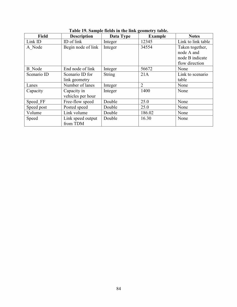
84

Table 19. Sample fields in the link geometry table. Field Description Data Type Example Notes

Link ID ID of link Integer 12345 Link to link table A_Node Begin node of link Integer 34554 Taken together,

node A and node B indicate flow direction

B_Node End node of link Integer 56672 None Scenario ID Scenario ID for

link geometry String 21A Link to scenario

table Lanes Number of lanes Integer 2 None Capacity Capacity in

vehicles per hour Integer 1400 None

Speed_FF Free-flow speed Double 25.0 None Speed post Posted speed Double 25.0 None Volume Link volume Double 186.02 None Speed Link speed output

from TDM Double 16.30 None

85

Table 20. Sample fields in the link volume table. Field Description Data type Example Notes

Link ID ID of link Integer 12345 Link to link table A_Node Begin node of

link Integer 34554 Taken together,

node A and node B indicate flow direction

B_Node End node of link Integer 56672 None Scenario ID Scenario ID for

this link geometry String 21A Link to scenario

table Lanes Number of lanes Integer 2 None Capacity Capacity in

vehicles per hour Integer 1400 None

Speed_FF Free-flow speed Double 25.0 None Speed Post Posted speed Double 25.0 None Volume Link volume Double 186.02 None Speed Link speed output

from TDM Double 16.30 None

V to C V/C ratio Double 0.95 None Density Traffic density on

link (vehicles/mi) Double 30.22 None

DEMANDS

Existing Practice

Different analysis resolutions require different traffic demand resolutions. Requirements for each of the four analysis resolutions are as follows:

• A traditional TDM typically outputs several types of trip tables. Production/attraction tables are intermediate person trip tables that are output from the trip generation and trip distribution process. O-D tables are person trip or vehicle trip tables that are used in the assignment process. Separate trip tables are produced by trip purpose and mode, and time-of-day trip tables are used for assigning passenger trips and vehicle trips to the transit and road networks. Different agencies have different time-of-day definitions. For example, a small agency might work only with daily trip tables, another agency might have a morning peak and an off-peak trip table, and a third agency may have separate trip tables for morning peak, afternoon peak, midday, and late night/early morning.

• Activity-based TDMs output individual trip records for individuals in a synthetic population that is intended to represent the population of the modeling region. Each trip record contains information that includes a weighting factor, travel mode, O-D, and some socioeconomic characteristics of the individual that could be used for more refined analyses (e.g., environmental justice analyses). Most activity models in use today rely on traditional network assignment procedures to get link volumes and level of service. As a result, these trip records are rolled up into traditional trip tables by mode and time of day.

86

• HCM-based tools typically analyze the peak 15-min volumes. An analyst may collect 1+ h of volume data during the peak morning and afternoon periods and then filter the data to isolate the heaviest 15-min interval for analysis.

• DTA models typically start with O-D matrices from a TDM and then adjust them to derive hourly or 15-min volumes.

• Microsimulation models often work with 15-min volumes that span the 1 to 2-h analysis period. Even though not frequently done, traffic variation every 1 or 5 min can be specified for each 15-min interval.

• Detailed traffic count data are kept for purposes of monitoring and validation.

In addition to the analysis practices mentioned, demand resolutions also vary in field data. For instance, many agencies collect and archive detector loop data. Raw data come in as time stamps which can then be aggregated to generate 1-min, 5-min, 15-min, hourly, 24-h, weekly, or monthly volumes. Due to processing speed and storage cost, not all of the data resolutions are stored nor are they retained for the same period of time.

Challenges

The brief summary in the previous section illustrates the difficulties encountered when attempting to integrate demand requirements for various modeling resolutions. Theoretically, traffic demands can be stored at the lowest common denominator (e.g., 20-s or 1-min volumes) to serve microsimulation analyses and then aggregated for other analysis resolutions. However, this approach is not currently practical for the following reasons:

• The original source of demand data for future years is from regional TDMs. Travel models output results by time period, which is typically at a very coarse resolution compared to that required by DTA and microsimulation models (e.g., a 3- to 4- h peak period). Current year traffic count data are typically used to break down travel model outputs into finer resolutions (i.e., 15 min or less).

• A large amount of 20-s or 1-min data can be unwieldy (i.e., difficult to store and work with).

• 20-s or 1-min data are not often collected and stored for all network links.

• Some link and node volumes are derived from land use data in TDMs. As a result, it is not possible to develop fine resolution volumes.

87

Proposed Structure

To satisfy various traffic demand levels, a demands table comprising of subsets for each modeling resolution is proposed. It is envisioned that demands in one subset may be derived from another subset, from analysis results, or from field data. Demand table fields are as follows:

• Table 21 shows the fields in the data table for activity model output. These tables are typically not used directly unless a more detailed analysis based on traveler socioeconomic characteristics is desired.

• Table 22 shows the fields in a data table for O-D model output from a traditional four-step model. These data are also produced by activity models as a precursor to the assignment phase of modeling.

• Table 23 shows the fields in a production/attraction table that is typical of an intermediate table in the traditional four-step modeling process.

88

• Table 24 shows the structure of a demand table for finer resolution analysis. This table is typically produced by breaking down travel model outputs at a coarser resolution (e.g., morning peak) using traffic count data.

• Table 25 shows the fields in the data table for traffic count data. These data may come from automated and manual field measurements.

89

Table 21. Demand for activity-based TDMs. Field Description Data Type Example Notes

Household ID Household ID number from synthetic sample

Integer 1001 None

Person ID Person ID number from synthetic sample

Integer 3 None

Weight Weighting factor for this person

Integer 2 None

Trip No Trip number Integer 2 None HH_Income Household

income of person in synthetic sample

Double 60,000.00 These are examples of household and person characteristics; other characteristics (e.g., ethnicity) could also be included

Person age Age of person in synthetic sample

Integer 44 None

Person sex Sex of person Enumeration Male None Activity origin Activity at origin Enumeration Home None Activity destination

Activity at destination

Enumeration Work None

TAZ_Origin Origin TAZ Integer 2433 None TAZ_Destination Destination TAZ Integer 1876 None Time begin Begin time of

trip Date and time 15:05 None

Time end End time of trip Date and time 15:40 None Mode Travel mode Enumeration Bus None

90

Table 22. O-D for assignment in regional TDM. Field Description Data Type Example Notes

Scenario ID ID of particular scenario

String 21A Link to scenario table

Time period Time period in which trip takes place

Enumeration Morning Definitions will depend on agency definitions of time periods

Trip purpose Trip purpose category

Enumeration Home to work Definitions will depend on agency definitions of trip purposes

Mode Travel mode Enumeration Auto driver Definitions will depend on agency definitions of modes

TAZ_Origin Origin TAZ Integer 2433 None TAZ_Destination Destination TAZ Integer 1876 None Trips Number of trips Double 23.59 None

Table 23. Production/attraction trip from four-step model. Field Description Data Type Example Notes

Scenario ID ID of particular scenario

String 21A Link to scenario table

Time period Time period in which trip takes place

Enumeration Morning Definitions will depend on agency definitions of time periods

Trip purpose Trip purpose category

Enumeration Home to work Definitions will depend on agency definitions of trip purposes

Mode Travel mode Enumeration Auto driver Definitions will depend on agency definitions of modes

TAZ_Production Production TAZ Integer 2433 None TAZ_Attraction Attraction TAZ Integer 1876 None Trips Number of trips Double 23.59 None

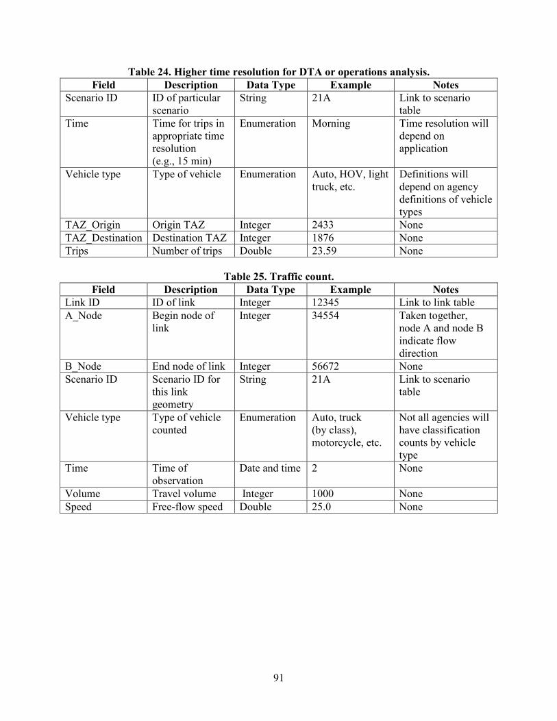
91

Table 24. Higher time resolution for DTA or operations analysis. Field Description Data Type Example Notes

Scenario ID ID of particular scenario

String 21A Link to scenario table

Time Time for trips in appropriate time resolution (e.g., 15 min)

Enumeration Morning Time resolution will depend on application

Vehicle type Type of vehicle Enumeration Auto, HOV, light truck, etc.

Definitions will depend on agency definitions of vehicle types

TAZ_Origin Origin TAZ Integer 2433 None TAZ_Destination Destination TAZ Integer 1876 None Trips Number of trips Double 23.59 None

Table 25. Traffic count. Field Description Data Type Example Notes

Link ID ID of link Integer 12345 Link to link table A_Node Begin node of

link Integer 34554 Taken together,

node A and node B indicate flow direction

B_Node End node of link Integer 56672 None Scenario ID Scenario ID for

this link geometry

String 21A Link to scenario table

Vehicle type Type of vehicle counted

Enumeration Auto, truck (by class), motorcycle, etc.

Not all agencies will have classification counts by vehicle type

Time Time of observation

Date and time 2 None

Volume Travel volume Integer 1000 None Speed Free-flow speed Double 25.0 None

92

TRANSIT

Existing Practice

Transit is coded as part of a regional transportation network. Transit is typically coded as a set of transit lines. Each transit line record contains a code for the mode (e.g., bus, rail, etc.), a code for the individual transit operator, a list of nodes along which the line runs, the service headway (with provision for specifying different peak and off-peak headways), and a code for the speed, which can be entered either as a factor related to the auto speed on a link or as an absolute speed (the latter is the format for transit lines with a separate right-of-way). Transit information also includes a fare matrix, which specifies TAZ-to-TAZ fares. Travel modeling software is becoming increasingly sophisticated with regard to transit, providing more detail on transit characteristics such as line specification, transit speeds, allowance for transit vehicle capacity limitations, and specification of allowable transfers between different transit routes..

Automated vehicle location (AVL) and automated passenger counting (APC) are being implemented on larger systems. AVL provides real-time transit vehicle arrival information at each transit stop or station. APC provides information on individual vehicle boardings and alightings at individual stops.

Google® has recently launched Google Transit®, which provides real-time transit information for over 120 transit operators in more than 475 cities in 36 U.S. States and 7 Canadian provinces. Development of this new application has entailed development of a new database schema called General Transit Feed Specification (GTFS) to allow transit operators to provide their information to Google® in a unified format. Because of its widespread and growing use, GTFS may provide a useful basis for defining the transit portion of the AMS database schema.

Challenges

Transit data are inherently complex. A full set of data on transit operations should include information on operator characteristics, route locations, stop locations, schedules, demand (e.g., demand by route and time of day and boardings and alightings by stop), and on-time performance versus schedule. Smaller operators do not collect all these data or may only collect them on a sample basis to fulfill Federal Transit Administration requirements for reporting to the National Transit Database.

Proposed Structure

The proposed structure consists of several tables that define transit routers and data on patronage by route. This structure is based in part on Google® GTFS.

Table 26 contains information on individual stops (i.e., location, zone, amenities, and routes that serve the stop and boardings and alightings at the stop by route).

93

Table 26. Sample fields in the stop table. Field Description Value

Stop ID ID number of stop Integer Stop description Description of stop Alphanumeric Stop location Stop location (latitude,

longitude) Point

Stop TAZ TAZ of stop Integer Stop type Indicates whether bus stop

or transit station Enumeration

Has bench Indicates whether stop has bench

Boolean

Has shelter Indicates whether stop has a shelter

Boolean

Boardings Average boardings at stop Numeric Alightings Average alightings at stop Numeric

Table 27 contains information on specific transit routes.

Table 27. Sample fields in the route table. Field Description Value

Operator Name of transit operator Alphanumeric Route ID ID number of route

(operator-specified) Alphanumeric

Route description Description of route Alphanumeric Mode Type of transit (e.g.,

commuter rail, heavy rail, light rail, rapid bus, express bus, local bus, etc.)

Enumeration

Average headway Average headway in minutes by time period (e.g., morning peak, midday, afternoon peak, or evening)

Numeric

Stop sequence Sequence of stop IDs that define the route

Vector of stop IDs

Hours operation Hours of operation Numeric

94

Table 28 identifies a set of zone-to-zone fares by transit operator. Fare information is used in the regional TDM as part of the demand forecasting process.

Table 28. Sample fields in the zone-to-zone fare table. Field Description Value

Operator Transit operator name Alphanumeric Route ID Individual route ID Alphanumeric Origin zone Origin TAZ Numeric Destination zone Destination TAZ Numeric Time of day Time period (e.g.,

morning peak, midday, and afternoon peak)

Enumeration

Normal fare Amount of fare Numeric Discount fare 1 Discounted fare for

category 1 (e.g., handicapped)

Numeric

Discount fare 2 Discounted fare for category 2 (e.g., youth)

Numeric

HOUSEHOLD TRAVEL SURVEYS

Existing Practice

Household travel surveys provide essential data on travel behavior for developing TDMs. Travel surveys are typically conducted by telephone for a sample of the population. Respondents are asked information about the household, persons in the household, vehicles in the household, and trips made by members of the household on a designated travel day. Some surveys collect data for multiple travel days.

A household travel survey is an expensive undertaking that is typically conducted at intervals of about 10 years by an MPO or a State transportation department. Current survey costs for a large-scale survey average $150–$200 per completed household sample.

The current trend has caused some household travel surveys to be activity-based where information is sought on activity schedules, whether at home or away from home. Trips are treated as special activities.

Challenges

Household travel survey datasets are complex and difficult to analyze. While they can be used to provide information for specific transportation studies, they are seldom used for these purposes because of the particular data analysis skills required to assemble and analyze the data. Household travel surveys data typically contain the following four types of files:

• Household file: Information on the household as a whole (e.g., location, vehicle ownership, income, etc.).

95

• Person file: Information on persons in the household (e.g., age, sex, relation to head of household, occupation status, etc.).

• Vehicle file: Information on vehicles in the household (make, model, year, mileage, owned or leased, etc.).

• Trip file (or activity file): A file of records on individual trips or activities. Each record contains activity type, begin time, and end time. If the record is for a trip, information includes mode, fare paid, type of parking, and vehicle occupancy.

Travel survey data typically require a large amount of time and effort for preprocessing. If the survey is activity-based, trip information must be selected from the activity file for use in travel modeling. Trip data are often further preprocessed. For example, if a person walks to transit, rides transit to a transfer point, transfers to another transit vehicle, and then walks to the destination, those are recorded as four separate trips in the trip file, but they must be linked together into a single trip (coded as a “transit, walk access” mode). Other types of trips may be linked to provide more accurate information (e.g., if a person makes a short stop on the way to work to buy coffee, the stop is sometimes linked, and the two trips are treated as a single home-work trip).

Proposed Structure

The proposed structure consists of a set of tables corresponding to the files in a typical household travel survey dataset (see table 29 through table 32). In addition, there would be a processed trip file that contains a set of trips that can be used directly for travel modeling or other travel analysis purposes.

Table 29. Sample fields in the household table. Field Description Value

Household ID ID of household (used to link to person and trip files)

Numeric

Location Household latitude and longitude

Point code

N_Persons Number of persons in the household

Numeric

N_Veh Number of vehicles in the household

Numeric

Income Household income Numeric Zone Zone where

household is located Numeric

96

Table 30. Sample fields in the person table. Field Description Value

Household ID ID of household Numeric Person ID ID number of person Numeric Relation Relation to head of

household Enumeration

Age Age Numeric Sex Sex Enumeration Occupation status Occupation status of

person (working, student, retired, homemaker)

Enumeration

Work loc Zone where workplace is located

Numeric

Handicapped Whether person has a handicap that limits ability to use transit

Boolean

Table 31. Sample fields in the vehicle table.

Field Description Value Household ID ID of household Numeric Make Make of vehicle Alphanumeric Model Vehicle model Alphanumeric Body type Vehicle body type Enumeration Year Model year of vehicle Numeric Mileage Miles on vehicle at

time of survey Numeric

Owned Is vehicle owned, leased, or provided by company

Enumeration

Fuel Fuel type of vehicle (e.g., gas, diesel, or hybrid)

Enumeration

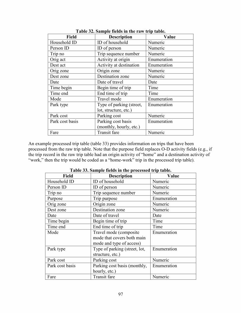
97

Table 32. Sample fields in the raw trip table. Field Description Value

Household ID ID of household Numeric Person ID ID of person Numeric Trip no Trip sequence number Numeric Orig act Activity at origin Enumeration Dest act Activity at destination Enumeration Orig zone Origin zone Numeric Dest zone Destination zone Numeric Date Date of travel Date Time begin Begin time of trip Time Time end End time of trip Time Mode Travel mode Enumeration Park type Type of parking (street,

lot, structure, etc.) Enumeration

Park cost Parking cost Numeric Park cost basis Parking cost basis

(monthly, hourly, etc.) Enumeration

Fare Transit fare Numeric An example processed trip table (table 33) provides information on trips that have been processed from the raw trip table. Note that the purpose field replaces O-D activity fields (e.g., if the trip record in the raw trip table had an origin activity of “home” and a destination activity of “work,” then the trip would be coded as a “home-work” trip in the processed trip table).

Table 33. Sample fields in the processed trip table. Field Description Value

Household ID ID of household Numeric Person ID ID of person Numeric Trip no Trip sequence number Numeric Purpose Trip purpose Enumeration Orig zone Origin zone Numeric Dest zone Destination zone Numeric Date Date of travel Date Time begin Begin time of trip Time Time end End time of trip Time Mode Travel mode (composite

mode that covers both main mode and type of access)

Enumeration

Park type Type of parking (street, lot, structure, etc.)

Enumeration

Park cost Parking cost Numeric Park cost basis Parking cost basis (monthly,

hourly, etc.) Enumeration

Fare Transit fare Numeric

98

TRAVEL MODEL OUTPUTS

Existing Practice

TDMs produce a number of different types of data that can be used for further analysis. Example outputs include the following:

• Trip tables: Number of trips by O-D pair by mode, trip purpose, and time of period.

• Skim tables: Travel times between zones by mode and time period. Transit skim tables typically include subfields for in-vehicle time, access time, wait time, and transfer time.

• Assignment tables: Number of vehicles by type (and transit passengers) on links in the travel network and travel speeds by time period.

Challenges

Travel models produce a large amount of output data that are typically kept in a format proprietary to the individual software vendor of the travel modeling software. Most travel modeling software packages are capable of exporting data into other formats (e.g., text, database, or spreadsheet). There is currently no standard practice for managing outputs from different travel modeling software packages.

Activity-based models produce outputs of individual trips for each person in a synthetic sample on which the model operates. The individual records contain information on characteristics of the person and the household so that outputs can be summarized by socioeconomic characteristics for purposes of equity analysis. These records can also be summarized into traditional trip tables like those produced by trip-based TDMs.

Proposed Structure

The proposed structure consists of a set of tables corresponding to travel model outputs. For trip-based models, the output will consist of a set of trip tables, zone-to-zone skims, and link assignments. Examples are shown in table 34 through table 36.

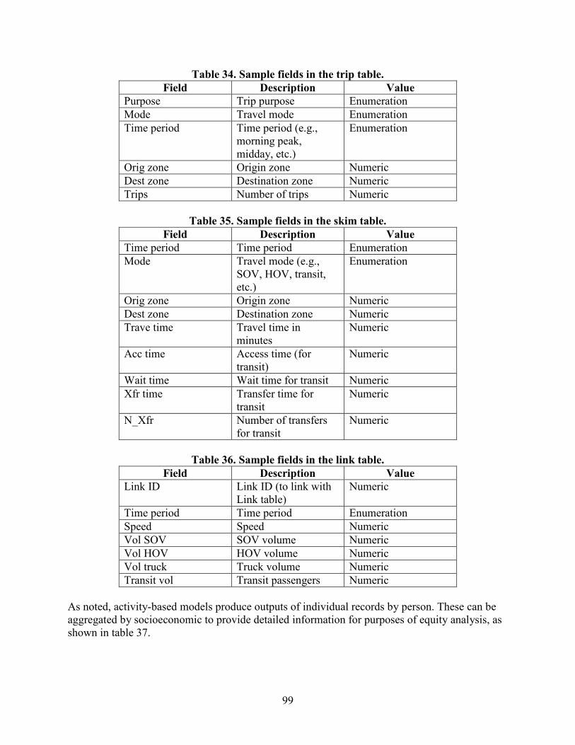
99

Table 34. Sample fields in the trip table. Field Description Value

Purpose Trip purpose Enumeration Mode Travel mode Enumeration Time period Time period (e.g.,

morning peak, midday, etc.)

Enumeration

Orig zone Origin zone Numeric Dest zone Destination zone Numeric Trips Number of trips Numeric

Table 35. Sample fields in the skim table.

Field Description Value Time period Time period Enumeration Mode Travel mode (e.g.,

SOV, HOV, transit, etc.)

Enumeration

Orig zone Origin zone Numeric Dest zone Destination zone Numeric Trave time Travel time in

minutes Numeric

Acc time Access time (for transit)

Numeric

Wait time Wait time for transit Numeric Xfr time Transfer time for

transit Numeric

N_Xfr Number of transfers for transit

Numeric

Table 36. Sample fields in the link table.

Field Description Value Link ID Link ID (to link with

Link table) Numeric

Time period Time period Enumeration Speed Speed Numeric Vol SOV SOV volume Numeric Vol HOV HOV volume Numeric Vol truck Truck volume Numeric Transit vol Transit passengers Numeric

As noted, activity-based models produce outputs of individual records by person. These can be aggregated by socioeconomic to provide detailed information for purposes of equity analysis, as shown in table 37.

100

Table 37. Sample fields in the activity-based model table. Field Description Value

Person ID Synthetic sample number

Numeric

Age Age of person Numeric Sex Sex of person Enumeration Income Household income

category Enumeration

Weight Expansion factor for person trip record

Numeric

Orig zone Origin zone Numeric Dest zone Destination zone Numeric Act orig Activity at origin Enumeration Act dest Activity at destination Enumeration Time begin Begin time of trip Time Time end End time of trip Time Mode Travel mode Enumeration Fare Transit fare paid Numeric Park cost Parking cost Numeric

MOES

Existing Practice

MOEs are typically compiled for a node, a link, a corridor, a zone, or an entire network. Depending on the analysis level, MOEs can be generic or comprehensive. Some common MOEs include the following:

• MOEs for nodes: V/C ratio, average delay, entering volume, etc.

• MOEs for links: V/C ratio, density, queue, delay, speed, travel time, number of stops, number of lane changes, vehicle-miles traveled, emissions, fuel consumption, etc.

• Path/corridor: Travel time, queue, delay, progression, vehicle-miles traveled, number of lane changes, number of stops, etc.

• Network: Average speed, total vehicle-miles traveled, total vehicle-hours of delay, total vehicle-hours of move time, total fuel consumption, total emissions, etc.

Challenges

Some challenges with MOEs include the following:

• Some link MOEs can potentially be aggregated to generate path and network MOEs. Space can be saved at the expense of computational speed.

101

• Emerging MOEs for reliability, safety, and sustainability have yet to be incorporated into mainstream AMS tools.

Proposed Structure

The MOEs table is proposed to comprise a number of subset tables, each of which contains MOEs for node, link, path, zone, and network respectively. Table 38 through table 41 show examples of these subsets.

Table 38. Subset table with sample MOE fields for nodes. Field Description Value Notes

Node ID Node number or ID Integer None Intervals Number of analysis

intervals with analysis period

Integer None

vc V/C ratio averaged for analysis period and each time interval

Numerical Avg_vc, vc_t1, vc_t2...

Delay Average delay for analysis period and each time interval

Numerical Avg_d, d_t1, d_t2...

Enter_vol Total entering volume (vehicles per hour)

Numerical Total_vol, v_t1, v_t2...

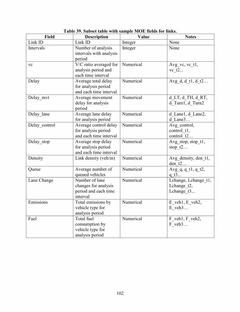
102

Table 39. Subset table with sample MOE fields for links. Field Description Value Notes

Link ID Link ID Integer None Intervals Number of analysis

intervals with analysis period

Integer None

vc V/C ratio averaged for analysis period and each time interval

Numerical Avg_vc, vc_t1, vc_t2...

Delay Average total delay for analysis period and each time interval

Numerical Avg_d, d_t1, d_t2…

Delay_mvt Average movement delay for analysis period

Numerical d_LT, d_TH, d_RT, d_Turn1, d_Turn2

Delay_lane Average lane delay for analysis period

Numerical d_Lane1, d_Lane2, d_Lane3…

Delay_control Average control delay for analysis period and each time interval

Numerical Avg_control, control_t1, control_t2…

Delay_stop Average stop delay for analysis period and each time interval

Numerical Avg_stop, stop_t1, stop_t2…

Density Link density (veh/m) Numerical Avg_density, den_t1, den_t2…

Queue Average number of queued vehicles

Numerical Avg_q, q_t1, q_t2, q_t3...

Lane Change Number of lane changes for analysis period and each time interval

Numerical Lchange, Lchange_t1, Lchange_t2, Lchange_t3...

Emissions Total emissions by vehicle type for analysis period

Numerical E_veh1, E_veh2, E_veh3…

Fuel Total fuel consumption by vehicle type for analysis period

Numerical F_veh1, F_veh2, F_veh3…

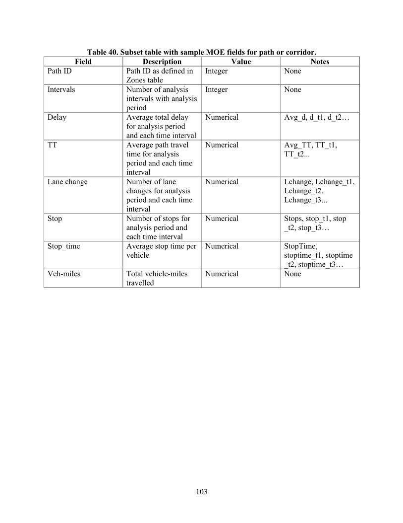
103

Table 40. Subset table with sample MOE fields for path or corridor. Field Description Value Notes

Path ID Path ID as defined in Zones table

Integer None

Intervals Number of analysis intervals with analysis period

Integer None

Delay Average total delay for analysis period and each time interval

Numerical Avg_d, d_t1, d_t2…

TT Average path travel time for analysis period and each time interval

Numerical Avg_TT, TT_t1, TT_t2...

Lane change Number of lane changes for analysis period and each time interval

Numerical Lchange, Lchange_t1, Lchange_t2, Lchange_t3...

Stop Number of stops for analysis period and each time interval

Numerical Stops, stop_t1, stop _t2, stop_t3…

Stop_time Average stop time per vehicle

Numerical StopTime, stoptime_t1, stoptime _t2, stoptime_t3…

Veh-miles Total vehicle-miles travelled

Numerical None

104

Table 41. Subset table with sample MOE fields for subarea and entire network. Field Description Value Notes

Zone ID Path ID as defined in Zones table

Integer “All” for all zones

Delay Total vehicle-hours of delay for analysis period and each time interval

Numerical d, d_t1, d_t2…

Del_Mile Average vehicle delay per mile

Numerical d-mile, d-mile_t1, d-mile_t2, d-mile_t3…

Move Total vehicle-hours of move time for analysis period and each time interval

Numerical Move, Move_t1, Move_t2…

Speed Average vehicle speed in zone

Numerical Speed, Speed_t1, Speed _t2, Speed _t3…

Emissions Total emissions by vehicle type for analysis period

Numerical E_veh1, E_veh2, E_veh3…

Fuel Total fuel consumption by vehicle type for analysis period

Numerical F_veh1, F_veh2, F_veh3…

Veh-miles Total vehicle-miles traveled

Numerical None

SCENARIOS

Existing Practice

An analysis of scenarios, alternatives, or options is a common requirement in all transportation planning, operations, and improvement projects. A few analysis tools allow the analyst to set up scenarios within the base analysis; however, the majority of analysis tools requires the analyst to make a copy of the base analysis before experimenting with changes in the network, traffic control, or demands. The following examples highlight scenarios typically encountered:

• Modification of timing and phasing to optimize signal operation.

• Modification of existing traffic control device (e.g., replacing a stop control with a signal or roundabout).

• Addition of capacity to an existing link and a series of links.

• Addition of new link(s) to the network.

• Conversion of one-way to two-way operations or vice versa.

105

• Implementation of toll or road pricing on existing link(s).

• Evaluation of traffic control strategies at work zones.

Challenges

Modifications of properties of existing nodes or links can more easily be tracked than the addition of new links and nodes. When a new link or node is added, traffic assignment, volumes, traffic control, and zones can all potentially be affected. The problem becomes exponentially challenging when more than one link and node are added. Because links and nodes have different properties, two separate tables will be required to store changes made to both.

Proposed Structure

The purpose of the scenario table is to automatically keep track of modifications made to the base file while keeping the base file intact for comparison purposes. The proposed table has a subset table for scenarios related to links and another subset for scenarios related to nodes. For scenarios involving new links and nodes, the analyst can employ the traditional approach of making copies of the base analysis. (See table 42 and table 43). Typical scenario setup and work flow are envisioned as follows:

• The analyst can set up one or more scenarios. Changes to links will be stored in the scenario link subset table, and changes to nodes will be stored in the scenario node subset table. One scenario can include only the link subset, the node subset, or both.

• The analyst can run the base analysis by itself or with one of the scenarios activated.

• Instances of MOE tables will be generated for scenarios analyzed and to enable cross comparison of scenarios.

106

Table 42. Subset table with sample scenario fields for links. Field Description Value Notes

Scenario ID Scenario ID Alphanumeric None Scenario_Type Scenario types Alphanumeric Pricing/Work_Zone/Incident/VMS Indifference Indifference band

(DTA) Numerical None

Threshold Threshold bound (DTA)

Numerical None

Pre-trip Pre-trip assignment (DTA)

Alphanumeric Random/best

Link ID Link number or ID

Integer None

Effective_t Effective time (start and end)

Alphanumeric Start_time, End_time

Toll_dist Distance-based toll ($/lane-mile)

Alphanumeric $_LOV, $_HOV, $_Truck

Toll_link Link-based toll ($/link)

Alphanumeric $_LOV, $_HOV, $_Truck

WZ Characteristics of work zone

Alphanumeric Lane_closed, speed_limit, discharge, length

Incident Characteristics of incident

Alphanumeric Lane_closed, length

VMS Variable message sign

Alphanumeric Speed/Detour/Congestion/…

Meter Ramp metering Alphanumeric Stop_bar, method, max_rate, min_rate, lanes

Parking On-street parking Alphanumeric Location, length, duration, and frequency

VMS = Variable message sign. LOV = Low-occupancy vehicle.

107

Table 43. Subset table with sample scenario fields for nodes. Field Description Value Notes

Scenario ID Scenario ID Alphanumeric None Scenario_Type Scenario types Alphanumeric Signal/stop-control/

closed Indifference Indifference band

(DTA) Numerical None

Threshold Threshold bound (DTA)

Numerical None

Pre-trip Pre-trip assignment (DTA)

Alphanumeric Random/best

Node ID Node number or ID Integer None Effective_t Effective time (start

and end) Alphanumeric Start_time, End_time

Signal Phasing and timing parameters

Alphanumeric None

Stop Stop control Alphanumeric Stop_Approach1 (Y/N), Stop_Approach2 (Y/N)…

Roundabout Roundabout control Alphanumeric None Closure Intersection closed,

detour required Alphanumeric None

SIGNAL CONTROL

Existing Practice

Signal operations and settings are traditionally simplified before being entered in an analysis tool. In most analysis tools, the ring and barrier setup is coded as sequential phases. Timing parameters such as minimum initial, splits, etc. are simplified as green, yellow, and all-red, and most controller settings such as red rest, recall mode, gap, etc. are ignored.

Challenges

Signal control challenges include the following:

• The traditional approach to simplify the signal settings for analysis cannot adequately depict advanced features (e.g., complex overlap phasing, priority treatment, dedicated pedestrian, or bicycle phase).

• Most if not all signal controllers are built modularly. A fully loaded signal cabinet can have many advanced functions and features that a basic controller lacks. Capturing everything in the data structure can be overwhelming.

108

• Adaptive signal control is becoming increasingly popular. A variety of adaptive approaches already exist as well as controllers and their detection methods and requirements.

• Several standards for signal controller exist.

Proposed Structure

It is proposed that the data structure for signal control adopts the National Electrical Manufacturers Association standards and includes all typical settings that directly control the signal head’s display and functions. This is shown in table 44 and table 45.

Table 44. Signal control table with sample fields. Field Description Data type Example Notes

Scenario ID Scenario ID for this zone (e.g., year, land use alternative)

String 21A Link to scenario table

Node ID ID of nodes with signal control

Integer 12345 Link to Node table

Control type Signal controller mode (e.g., pre-timed, actuated, coordinated, or adaptive)

Integer 1 1: pre-timed; 2: actuated; 3: coordinated; 4: adaptive

Offset Signal offset for signals in coordination

Double 15.0 None

Yield Reference point for yield

Double 30.0 None

Reference Reference phase for coordination

Integer 2 None

109

Table 45. Signal phasing table with sample fields. Field Description Data Type Example Notes

Node ID ID of nodes with signal control

Integer 12345 Link to signal table

Interval ID Time interval where entries below are applicable

Integer 1 Interval duration is defined in another table

Phase ID Phase 1 through 8 in the dual ring barrier control structure

Integer 2 None

Link ID Subject approach of movements in Phase ID

Integer 2 Link to link table

Movement Phase movements (left, through, right, diagonal 1, or diagonal 2)

String L1 L, T, R, 1, or 2

Min Green Minimum green time for phase ID

Double 15.0 None

Max Green Maximum green time for phase ID

Double 30.0 None

Veh Ext Vehicle extension Double 3.0 None Time before reduce

Duration before gap reduction

Double 7.0 None

Time to reduce Reduction amount Double 15.0 None Min gap Minimum gap Double 3.0 None Yellow Yellow or amber

interval Double 4.0 None

All red All-red interval Double 2.0 None Recall Recall mode Integer 1 0: No; 1: Yes Walk Pedestrian “Walk”

phase Double 10.0 None

Don’t walk Pedestrian “Don't Walk” phase

Double 15.0 None

Ped calls Pedestrian activation Integer 1 0: No; 1: Yes Dual entry Dual entry indicator Integer 1 0: No; 1: Yes Inhibit max Allows controller to

“gap out” but not “max out”

Double 45 None

110

VEHICLE TRAJECTORIES

Existing Practice

Vehicle trajectories can range from very detailed second-by-second lane-by-lane trajectory generated by microsimulation models to grossly estimated trajectories in macro- or HCM-based tools in order to estimate emissions and fuel consumptions. In microsimulation, trajectories are generated for individual vehicles and used in animation and estimation of the most detailed MOEs if needed.

Challenges

For a large network analyzed over a long period of time, the amount of vehicle trajectory data generated can be unwieldy.

Proposed Structure

Table 46 describes the structure for vehicle trajectory data.

Table 46. Vehicle trajectory table with sample fields. Field Description Value Notes

Veh ID Vehicle ID Integer None Path Series of links that

the vehicle traverse Integer Link_a, Link_b, Link_c,

Link_d... Veh type Vehicle type Alphanumeric Car/HOV/Truck/Bus/BRT/… Speed Average vehicle

speed per link Numerical Speed_a, Speed _b, Speed

_c... T time Average vehicle

travel time per link Numerical TT_a, TT_b, TT_c, TT_d...

Accel Average link-based vehicle acceleration

Numerical Acc_a, Acc _b, Acc _c, Acc _d...

Decel Average link-based vehicle acceleration

Numerical Dec_a, Dec_b, Dec_c, Dec_d...

111

CONFIGURATION

Existing Practice

Each analysis tool has certain assumptions and default parameters to carry out the analysis. Software may or may not allow the analyst to override these assumptions and defaults. Some of these settings are specific to software, some are specific to a theory employed by the software, and others are specific to a corridor or network being analyzed. Two examples are presented to illustrate challenges.

Example 1: Configurations for CORSIMTM

Sample configuration parameters required by CORSIMTM are provided.(10) The listed parameters are for illustrative purposes and are not all-inclusive.

Configuration parameters common to microsimulation include the following:

• Initialization period: Random seeds and vehicle entry headway distributions.

• Analysis period: Start time, number of intervals, and interval duration.

• Analysis description: Analyst name, agency, analysis date, unique identification, project/scenario description, and link name.

• Output trajectory file: For each probe vehicle, a probe file from CORSIMTM records its entrance and exit time, vehicle ID, path ID, as well as the node number sequence.

Configuration parameters specific to a car-following lane-changing theory include the following:

• Mean startup delay, mean discharge headway, and queue discharge distribution.

• Car following sensitivity and driver acceleration/deceleration.

• Acceptable gap distribution, start-up lost-time distribution, spillback probabilities, lane change behavior, driver familiarity, free flow speed distribution, and left-turn behavior.

Configuration parameters specific to CORSIMTM include the following:

• Random seeds for freeway and arterial headways, vehicle types and properties, fuel consumption and emission rates, and pre-timed signal transition algorithm.

• Distribution of discharge headway, distribution of bus dwell time, distribution of interaction for pedestrian delay, short-term event, and interchange O-D.

• Format of cumulative reports.

• User interface including grid, project directory, color, and node numbering.

112

Configuration parameters specific to the analysis include the following:

• Analysis period: Start time, number of intervals, and interval duration.

• Analysis description: Analyst name, agency, analysis date, unique identification, project/scenario description, and background file.

Example 2: Configurations for DynusT

Sample configuration parameters required by DynusT include the following (the listed parameters are for illustrative purposes and are not all-inclusive):

• Simulation period, number of iterations, number of simulation intervals per aggregation, vehicle generation mode, and convergence threshold.

• Timing plans, left-turn capacity, two-way stop control capacity, four-way stop control capacity, yield control capacity, traffic flow models, and grade length passenger car equivalent.

• User interface including grid, color scheme, background file, various output files, software version, and unit (English/metric).

Challenges

Challenges include the following:

• Different model resolutions are based on different theories which have different configuration requirements.

• Software tools within the same resolution can be based on different theories.

• Software tools based on the same theory can have their own interpretation, assumptions, and default values.

Proposed Structure

As anticipated, configuration parameters vary significantly from one resolution to another and from model to model within one resolution. It is proposed to include the few common parameters among software packages in the configuration table and allow parameters specific to software to be added and stored on an as-needed basis (see

113

table 47).

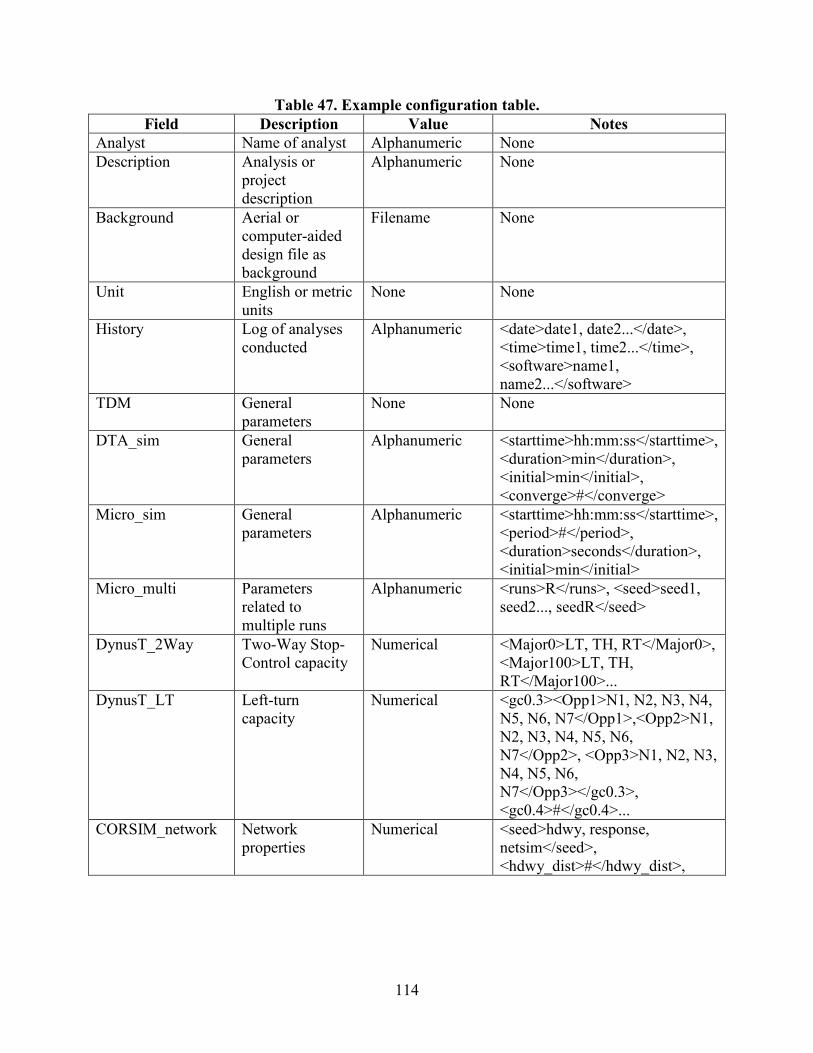
114

Table 47. Example configuration table. Field Description Value Notes

Analyst Name of analyst Alphanumeric None Description Analysis or

project description

Alphanumeric None

Background Aerial or computer-aided design file as background

Filename None

Unit English or metric units

None None

History Log of analyses conducted

Alphanumeric <date>date1, date2...</date>, <time>time1, time2...</time>, <software>name1, name2...</software>

TDM General parameters

None None

DTA_sim General parameters

Alphanumeric <starttime>hh:mm:ss</starttime>, <duration>min</duration>, <initial>min</initial>, <converge>#</converge>

Micro_sim General parameters

Alphanumeric <starttime>hh:mm:ss</starttime>, <period>#</period>, <duration>seconds</duration>, <initial>min</initial>

Micro_multi Parameters related to multiple runs

Alphanumeric <runs>R</runs>, <seed>seed1, seed2..., seedR</seed>

DynusT_2Way Two-Way Stop-Control capacity

Numerical <Major0>LT, TH, RT</Major0>, <Major100>LT, TH, RT</Major100>...

DynusT_LT Left-turn capacity

Numerical <gc0.3><Opp1>N1, N2, N3, N4, N5, N6, N7</Opp1>,<Opp2>N1, N2, N3, N4, N5, N6, N7</Opp2>, <Opp3>N1, N2, N3, N4, N5, N6, N7</Opp3></gc0.3>, <gc0.4>#</gc0.4>...

CORSIM_network Network properties

Numerical <seed>hdwy, response, netsim</seed>, <hdwy_dist>#</hdwy_dist>,

115

CORSIM_veh Vehicle type characteristics in CORSIMTM

Numerical <veh1>perf, length, occ, hdwy, jerk, decel1, decel2, s_car, s_HV, s_transit, s_hov, f_car, f_HV, f_transit, f_hov, </veh1>, <veh2>…</veh2>...

Vissim_veh Vehicle type characteristics in PTV Vissim®

Numerical <car>width, occ, color, max_accel, des_accel, max_del, des_del</car>, <hov>…</hov>,

Vissim_behavior Driving behavior parameters in PTV Vissim®

Numerical <urban>min_ahead, max_ahead, Obs_veh, min_back, max_back, inattention, inattention_prob, <model>standstill, safety, multi_safety</model>, <lanechange>…</lanechange>... </car>, <fwy>…</fwy>, <footpath>…</footpath>

117

REFERENCES

1. Committee for Determination of the State of the Practice in Metropolitan Area Travel Forecasting. (2007). Special Report 288: Metropolitan Travel Forecasting: Current Practice and Future Direction, Transportation Research Board, Washington DC.

2. Transportation Research Board. (2010). Highway Capacity Manual 2010, 5th Ed., National Research Council, Washington, DC.

3. Daiheng, N. (2006). “Challenges and Strategies of Transportation Modeling and Simulation Under Extreme Conditions,” International Journal of Emergency Management, 3(4), 298–312.

4. Sbayti, H. and Roden, D. (2010). Best Practices in the Use of Micro Simulation Models, NCHRP Project 8-36, Task 90, National Cooperative Highway Research Program, Washington, DC.

5. Bikowitz, E. and Ross, S. (1982). “Evaluation and Improvement of Inductive Loop Detectors,” Transportation Research Record 841, Transportation Research Board, Washington, DC.

6. Google Fusion Tables. (2013). Google Fusion Tables® data exported from NeXTA. Data date: October 12, 2011. Scale: 100 percent. Generated by: Jeffrey Taylor via Google Fusion Tables. Obtained from: https://www.google.com/fusiontables/DataSource?docid=1DFC qEWG2jTOZQYWUsm8c9o91uRbcxJeNEJ1tf7o#rows:id=1. Generated June 18, 2013.

7. Google Maps. (2013). Example network plotted using Google Maps®. Data date: October 12, 2011. Scale: 100 percent. Generated by: Jeffrey Taylor via Google Maps online. Obtained from: http://maps.google.com/. Generated June 18, 2013.

8. Google Fusion Tables. (2013). Example scatter plot using Google Fusion Tables®. Data date: October 12, 2011. Scale: 100 percent. Generated by: Jeffrey Taylor via Google Fusion Tables. Obtained from: https://www.google.com/fusiontables/DataSource?docid=1DFCq EWG2jTOZQYWUsm8c9o91uRbcxJeNEJ1tf7o#chartnew:id=4. Generated June 18, 2013.

9. Google Maps. (2013). Tucson Network MOE visualization. Data date: October 3, 2012. Scale: 100 percent. Generated by: Jeffrey Taylor via Google Maps. Obtained from: http://maps.google.com/. Generated June 18, 2013.

10. Holm, P., et al. (2007). Traffic Analysis Toolbox Volume IV: Guidelines for Applying CORSIM Microsimulation Software, Report No. FHWA-HOP-07-079, Federal Highway Administration, Washington, DC.

HRDo-20/08-13(WEB)E