the effects of alcohol consumption on earnings in...
TRANSCRIPT

THE EFFECTS OF ALCOHOL CONSUMPTION ON
EARNINGS IN AUSTRALIA
Gwen Cruise
Honours Thesis
Bachelor of Arts/Bachelor of Economics (Honours)
Supervisor: Garry Barrett
9th June 2009

2
DECLARATION I hereby declare that this submission is my own work and any contributions or materials
by other authors used in this thesis have been appropriately acknowledged. This thesis
has not been previously submitted to any other university or institution as part of the
requirements for another degree or award.
Gwen Cruise 9th June 2009

3
ACKNOWLEDGEMENTS I would like to thank my supervisor, Associate Professor Garry Barrett, for his support
and assistance throughout my Honours year, for his always timely advice and for writing
a paper that inspired my topic. I’d like to thank Associate Professor Peter Kriesler for
helping me to get started in Honours. Thanks also to Professor Denzil Fiebig for helping
to make econometrics seem intuitive and to Dr Shiko Maruyama for helping to develop
my interest in this area.
A big thankyou to both cohorts of Honours students with whom I’ve shared my Honours
year for making the experience that much easier. Finally, thanks to my family and
friends, who have seen a lot less of me since thesis writing began, but who have offered
all the support I could have hoped for.

4
TABLE OF CONTENTS
ABSTRACT ............................................................................................................................... 7
1. INTRODUCTION ........................................................................................................... 8
2. BACKGROUND TO “SAFE” DRINKING LEVELS ............................................... 13
3. LITERATURE REVIEW ............................................................................................. 16
4. THEORETICAL MODEL ............................................................................................ 21
5. ECONOMETRIC APPROACH ..................................................................................... 26
5.1 ESTIMATION TECHNIQUE .................................................................................. 26
5.2 EARNINGS DECOMPOSITIONS .......................................................................... 27
6. DATA ............................................................................................................................. 29
6.1 DATA BACKGROUND .......................................................................................... 29
6.2 THE SAMPLE.......................................................................................................... 30
6.3 DEPENDENT VARIABLES ................................................................................... 32
6.3.1 LOG EARNINGS EQUATION ........................................................................ 32
6.3.2 SELECTION (DRINKING STATUS) EQUATION ......................................... 34
6.4 INSTRUMENTAL VARIABLES............................................................................ 37
6.5 INDEPENDENT VARIABLES ............................................................................... 43
7. STATISTICAL ANALYSIS .......................................................................................... 45
7.1 RESULTS USING OLS AND DRINKING STATUS DUMMIES......................... 45
7.2 ESTIMATION USING THE HECKMAN SELECTION MODEL ........................ 47
7.2.1 RESULTS OF THE SELECTION REGRESSION ........................................... 47
7.2.2 RESULTS FOR LOG EARNINGS EQUATIONS ............................................ 51
7.3 EARNINGS DECOMOPOSITIONS ....................................................................... 55
7.4 SENSITIVITY ANALYSIS OF THE HECKMAN SELECTION ESTIMATION 56
7.4.1 EXOGENOUS SELECTION ........................................................................... 57
7.4.2 EXCLUSION OF RELIGIOUS ATTENDANCE ............................................. 58
7.4.3 DRINKING STATUS DEFINITION ................................................................ 60
8. CONCLUSION .............................................................................................................. 65
9. APPENDICES ................................................................................................................ 69
APPENDIX 1: COMPARISON OF MEANS FOR MISSING DATA ......................... 69
5
APPENDIX 2: SURVEY QUESTIONS ABOUT ALCOHOL CONSUMPTION ....... 70
........................................................................................................................................ 70
APPENDIX 3: SURVEY QUESTIONS ABOUT RELIGION ..................................... 71
APPENDIX 4: FULL LIST OF VARIABLES AND THEIR DEFINITIONS .............. 72
APPENDIX 5: LOG EARNINGS RESULTS ASSUMING EXOGENOUS SELECTION.................................................................................................................. 74
APPENDIX 6: LOG EARNINGS RESULTS (RELIGIOUS ATTENDANCE EXCLUDED) ................................................................................................................. 75
APPENDIX 7: HECKMAN SELECTION RESULTS USING NHMRC DEFINITION ................................................................................................................. 76
APPENDIX 8: HECKMAN SELECTION RESULTS USING ALTERNATIVE DEFINITION ................................................................................................................. 78
10. REFERENCES .............................................................................................................. 80

6
LIST OF TABLES Table 1: Summary statistics for ln earnings ............................................................................ 33
Table 2: Drinking Status Definition (percentage of sample) ................................................... 35
Table 3: Churning of Smoking Status (percentage of sample) ................................................ 39
Table 4: Mean Values for Instrumental Variables by Drinking Status .................................... 41
Table 5: Mean Values for Independent Variables by Drinking Status .................................... 44
Table 6: OLS Regression Results using Drinking Status Dummies ........................................ 46
Table 7: Results of Multinomial Logit Selection Equation ..................................................... 48
Table 8: Results of Log Earnings Regression by Drinking Status........................................... 53
Table 9: Earnings Decompositions .......................................................................................... 55
Table 10: Results of Multinomial Logit Selection Equation ................................................... 59
Table 11: Earnings Decompositions for Change in Drinking Status Definitions .................... 63

7
ABSTRACT The effects of alcohol consumption on health have been of interest to researchers in the
medical literature for some time now. This has spilled over into an interest in the economic
literature of the effects of alcohol consumption of earnings. The exact nature of this research
varies from the effect of alcohol on productivity for those in full-time work, to its effect on
labour market participation. This thesis contributes to the literature about the effect of alcohol
consumption on earnings through productivity and looks specifically at the issue using recent
Australian data.
This is the first research that has been done in this area using the Household Income and
Labour Dynamics Australia (HILDA) dataset. It also bases definitions of what is termed
heavy alcohol consumption on recently revised guidelines about safe drinking behaviour.
Using wave 7 of the HILDA dataset, an extension of the Heckman selection model is used to
estimate separate log earnings regressions for abstainers, moderate drinkers and heavy
drinkers. Earnings decompositions are then used to analyse whether differences in earnings
between drinker groups are attributable to differences in the average level of characteristics
or to differences in the productivity returns to those characteristics.
The results show that moderate drinkers receive an earnings premium relative to abstainers
that is largely attributable to productivity returns. Heavy drinkers receive a small earnings
penalty relative to moderate drinkers, although this is largely due to differences in
characteristics rather than differences in productivity returns. These results are found to be
sensitive to the definition of the different drinking status groups.

8
1. INTRODUCTION
In today’s society there is an increasing focus on wanting to maintain a healthy lifestyle.
Maintaining good health allows us to make the most of other areas in our lives, including
work, spending time with family or other leisure time. Smoking and obesity are frowned
upon, their negative health implications are widely known and government campaigns are in
place to promote awareness of their health impacts. Over recent years in Australia excessive
drinking has also been brought under the umbrella of bad health behaviour in public
discussion.
The current Federal government is making an effort to tackle our apparent culture of
excessive drinking. These efforts have included discussion of health warnings on alcohol
packaging (like those currently in place for tobacco products) and banning alcohol
sponsorship and advertising in professional sports (Sinclair, 2008b). In early 2008, new
policy initiatives in this area have included a commitment of $53 million to tackle this
apparent problem of binge drinking and, most recently, a tax on “alcopops” (Sinclair 2008a).
This attention coincides with recent downward revisions, by both American and Australian
national health bodies, to what is considered a safe level of drinking.
An important economic issue in relation to risky health behaviour is whether an investment in
our health, or human capital, through pursuing good health behaviour, corresponds to positive
effects in other areas of our lives. This thesis looks at one particular aspect of this problem,
whether drinking alcohol affects our human capital in a way that is reflected in work
productivity. As such, if alcohol consumption affects work productivity, this should be
reflected in the earnings of workers.

9
The debate about the health effects of alcohol makes this a somewhat complicated and, as
such, interesting analysis. There is unqualified acceptance that heavy drinking is damaging to
an individual’s health and personal relationships. A flipside to these known effects of heavy
drinking, there has also been active debate in the medical literature about whether low levels
of drinking are actually beneficial for health, in reducing stress, preventing cardiovascular
disease and potentially protecting against other diseases (Ashley et al, 2000; Castelnuovo et
al, 2002; Bryson et al, 2006).
Even more controversial is the debate about where the line can be drawn between safe and
unsafe drinking levels. However, it would seem that there does exist a U-shaped relationship
between alcohol consumption and health. The implication is that low levels of alcohol
consumption can afford health benefits, but as consumption increases its effects become
damaging, with a wide variety of potential health and psychological impacts, including
memory loss (Verster et al, 2003; Baglietto et al, 2006). These negative health effects act as a
disinvestment in human capital, hence it is expected that they will lead to lower levels of
earnings.
Alcohol’s status as a social drug also throws up other issues for consideration. A certain level
of alcohol consumption may act as an indication of social networking. People who drink
socially may be forming networks, particularly if that social drinking is done with work
colleagues. Therefore, a certain level of drinking may also have social networking benefits
that are reflected in earnings.
For my research, I have classified individuals as belonging to one of three different groups in
relation to their alcohol consumption: abstainers, moderate drinkers and heavy drinkers. The

10
reason for this is to try and separate the potentially positive productivity effects of a safe or
moderate level of drinking from the potentially negative effects of a heavy level of drinking.
This classification will also reflect the U-shaped effects of alcohol consumption discussed in
the medical literature.
In an economic sense, there are three main ways in which alcohol consumption may affect
earnings. First of all, it can affect the probability of actually being employed. Once employed,
it may affect productivity through on the job performance. It may also affect the level of
earnings attained as social networking may improve the likelihood of promotion. My research
focuses on the effect of alcohol consumption on the earnings of those already in full-time
employment. As such, my research does not deal with the issue of how alcohol consumption
affects the probability of being employed. Nor does it deal directly with its effect on the
probability of being promoted. Rather, it focuses on whether alcohol consumption affects the
earnings of workers, which may reflect either the effects of on the job performance or more
rapid promotion through the ranks as a result of social networking.
The model used in my research attempts to determine whether an individual’s drinking status,
as an abstainer, moderate drinker or heavy drinker, has an effect on their earnings. A
significant obstacle to the econometric modelling of this effect is that drinking status is
potentially endogenous to earnings. This endogeneity problem arises largely because workers
may self-select into drinking status. Another problem is that it is preferable to perform the
estimations with a form that is flexible enough to allow the returns to observable
characteristics to vary by drinking status, in order to compare the productivity returns
between drinker groups.

11
As such, I use a Heckman selection model to estimate three separate log earnings equations,
one for abstainers, one for moderate drinkers and one for heavy drinkers. By estimating these
three log earnings equations, it is possible to compare the returns to observable characteristics
for each drinker type. The Heckman selection model corrects for the non-random, truncated
samples that are created by dividing the original sample into three sub-groups. The variables
included in the exclusion restriction of the selection equation act as instrumental variables,
which control for the potential endogeneity problem. Following these log earnings
estimations, earnings decompositions are used to gain a sense of whether differences in
earnings between drinker types are atrributable to differences in the average level of
observable characteristics of each drinker group or whether they are due to the difference in
returns to those characteristics.
While similar studies have been done in Australia and abroad, they have used much older
data than that used for this research and they were published before the recent downwards
revisions of safe drinking levels. This study makes use of the Household Income and Labour
Dynamic in Australia (HILDA) dataset, which has not previously been used for this research
area. HILDA provides a rich source of variables relevant to the empirical modelling of this
issue, including potential instrumental variables. The data used by several Australian papers
in this area is now two decades old (Barrett, 2002 and Lye & Hirschberg, 2004). The data
source used for these papers was the National Health Survey (NHS) 1989-1990 performed by
the Australian Bureau of Statistics (ABS).
HILDA is arguably a richer source of data for this topic than the NHS and has the advantage
of providing data collected very recently. I am using wave 7 of the HILDA panel dataset.

12
This wave was collected in 2007 and had only been available for four months at the time of
submission.
This thesis also looks at the effects of drinking status on earnings in light of recently revised
safe drinking guidelines. Revised guidelines have been published by both the American
National Institutes of Health (NIH) and the Australian National Health and Medical Research
Council (NHMRC). Previous research by Hamilton & Hamilton (1997) and Barrett (2002)
had defined their demarcation between moderate and heavy drinking based on previous safe
drinking guidelines that were significantly more generous than the current ones.
The findings of this research reflect those of previous research in this area, showing that there
is an earnings premium to moderate drinking (Hamilton & Hamilton, 1997 & Barrett, 2002) .
This premium is largely the result of higher productivity returns to observable characteristics
for moderate drinkers over abstainers. There is also found to be a small earnings penalty for
heavy drinking relative to moderate drinking. However, this penalty is not large enough to
cancel out the positive earnings effects of alcohol consumption over abstention. This finding
reflects those of previous research that looks at the effects of general alcohol consumption on
earnings (Hamilton & Hamilton, 1997 & Barrett, 2002), but does not reflect the findings of
research focusing only on binge drinking (Keng & Huffman, 2002) . However, these results
are found to be sensitive to the definition of drinker types. For definitions of heavy drinking
that give a very low safe drinking threshold, these productivity returns disappear almost
entirely. For definitions of heavy drinking that give a very high threshold, these effects are
accentuated.
13
2. BACKGROUND TO “SAFE” DRINKING LEVELS
In Australia, safe drinking guidelines have been published by the National Health and
Medical Research Council (NHMRC). The NHMRC is a Federal Government peak body
responsible for, amongst other goals, “supporting health and medical research [and]
developing health advice for the Australian community” (NHMRC, 2009a). The most recent
NHMRC “Australian Guidelines: to reduce health risks from drinking” (2009b), published in
February 2009 are an update of previous guidelines published in 2001.
The NHMRC guidelines are based upon a literature review of epidemiological studies and
modelling based on a range of Australian data sources (NHMRC, 2009b, p.9). The current
guidelines specify that an acceptable level of alcohol consumption for healthy men and
women is no more than two standard drinks per day in order to prevent the lifetime risk of
harm from alcohol-related disease or injury. It also specifies that no more than four standard
drinks should be consumed on any single occasion in order to reduce the risk of alcohol-
related injury arising from that occasion, though this will still contribute to the lifetime risk of
harm (NHMRC, 2009b, p.2-3). In Australia, and under these guidelines, a standard drink is
defined as containing 10 grams of pure alcohol.
The 2009 guidelines are an update of “The Australian alcohol guidelines: health risks and
benefits” (NHMRC, 2001). In these 2001 guidelines, healthy drinking levels were defined
separately for men and women. For men, safe drinking was defined as an average of no more
than four standard drinks per day and no more 28 standard drinks per week, with strictly no
more than six standard drinks on any day and one to two alcohol free days per week.
14
For women the recommended levels were slightly lower with an average of no more than two
standard drinks per day and no more than 14 standard drinks per week, as well as a strict limit
of four standard drinks on any day and one to two alcohol free days per week (NHMRC,
2001, p. 6). The 2009 guidelines argue that safe drinking levels were revised downwards
based on research made available after publication of the 2001 guidelines and a new approach
to developing population health guidance (NHMRC, 2009, p. 1).
An alternative set of guidelines are those published by the US National Institutes of Health
(NIH), titled “Rethinking Drinking: Alcohol and your health” (NIH, 2009a). The NIH has
similar goals to those of the NHMRC in Australia, to act as “the steward of medical and
behavioural research for the Nation [and to apply] knowledge to extend healthy life and
reduce the burdens of illness and disability” (NIH, 2009b).
These guidelines also specify different levels of safe drinking for men and women. For men it
is recommended to have no more than four drinks on any one day and no more than 14 drinks
per week. Women are recommended to have no more than three drinks per day and no more
than seven drinks per week.
In these American guidelines a standard drink is classified as containing 14 grams of pure
alcohol. So, when converted to the Australian definition of a standard drink, the NIH
recommendations for men imply no more than 56 grams of pure alcohol on any one day, or
five to six Australian standard drinks, and no more than 196 grams of pure alcohol per week,
or between 19 and 20 Australian standard drinks per week. From here on, the term “standard
drink” will always refer to the Australian definition as this is the definition used by the
HILDA data.

15
I chose the current NIH classification of safe drinking levels as the basis for my preferred
demarcations between abstainers, moderate drinkers and heavy drinkers. In terms of this
analysis, the NIH guidelines offered two main advantages over other definitions. First of all,
it provided a limit to acceptable drinking levels across both the frequency and intensity
dimensions of alcohol consumption, unlike the current NHMRC guidelines or the definitions
used by Hamilton & Hamilton (1997) and Barrett (2002) which cap intensity only. Secondly,
it provided a middle ground for the intensity aspect of drinking between the very low levels
recommended by the current NHMRC guidelines and the quite high levels defined by
Hamilton & Hamilton (1997) and Barrett (2002). Nevertheless, the construction of this
variable is subject to sensitivity analysis as part of this research.

16
3. LITERATURE REVIEW
There is a small literature that looks specifically at the effects of alcohol consumption on
earnings. This literature is situated within two broader themes. The first of these looks at the
impact of alcohol consumption on earnings through its effect on labour market participation.
The second looks at the effects of alcoholism, smoking and other drug consumption on
earnings or labour market participation.
The idea of modelling the impact of alcohol consumption on earnings was first implemented
by Berger & Leigh (1988). Their empirical work uses the 1972-1973 Quality of Employment
Survey of US civilians aged 16 or over and working 20 or more hours a week. In order to
model this effect, the authors divided their sample between drinkers and non-drinkers, which
are then divided again between males and females. As a result, four separate log earnings
regressions are estimated using the two-stage Heckman selection model as developed by
Heckman (1979).
In order to compare the earnings between drinkers and non-drinkers, a type of earnings
decomposition is performed, comparing actual and predicted wages for both men and women.
The authors find that even after controlling for observable explanatory variables and selection
bias, drinkers earn higher wages than non-drinkers. The authors attribute this finding largely
to the possibility of moderate alcohol consumption having beneficial effects or to heavy
drinkers having to drop out of the labour force once they develop health problems.
Mullahy & Sindelar (1993) find a negative effect of alcoholism, as distinct from general
alcohol consumption, on earnings. This finding highlights that the model used by Berger &
Leigh (1988) may not be flexible enough to pick up the potentially negative effect of heavy

17
levels of drinking on earnings. Mullahy & Sindelar (1993) consider two impacts of
alcoholism on income. These are both the impact on the likelihood of working and the impact
on actual earnings, for those who are already working. The authors use a Heckman selection
model where the first step is a probit model estimation of whether an individual is in full-time
work and the second is a log earnings equation estimated using OLS.
The authors find that the first effect, that of alcoholism on the likelihood of working, is the
most economically significant one but that there is also a negative effect of alcoholism on
earnings after controlling for variables correlated with alcoholism. The seemingly
contradictory findings presented by Berger & Leigh (1988) and Mullahy & Sindelar (1993)
are the result of an analysis of different behaviours, the former looking at general alcohol
consumption and the latter at alcohol dependency. The implication is that there needs to be a
careful demarcation between the definition of drinking in what is deemed to be a healthy
quantity and drinking heavily, or to the point of dependency, when analysing the effects of
alcohol consumption on earnings.
The discrepancy between the findings of Berger & Leigh (1988) and Mullahy & Sindelar
(1993) clearly left room for further work to be done in modelling the expected negative
effects of heavy drinking and in the interpretation of the mechanisms through which alcohol
consumption affects earnings. Hamilton & Hamilton (1997) adapt the model used by Berger
& Leigh (1988) and extend it so that individuals are not classified simply as non-drinkers or
drinkers but as non-drinkers, moderate drinkers or heavy drinkers.
The idea for this extension is to allow for a U-shaped effect of alcohol consumption on
earnings, whereby the a priori expectation is that moderate drinkers experience the positive

18
earnings returns found by Berger & Leigh (1988) but heavy drinkers experience the negative
returns found by Mullahy & Sindelar (1993). The use of the Heckman selection model has
two-fold benefits in this work. First of all, it is possible to control for the potential
endogeneity of alcohol consumption and earnings through the use of instrumental variables in
the exclusion restriction of the first stage regression.
Secondly, by estimating a log earnings equation for each of the three sub-groups, it is then
possible to use the results, coupled with an earnings decomposition, to make pairwise
comparisons between the productivity returns to observable characteristics of each drinking
status group. Using this method, and focusing on the population of working males aged 25 to
59, Hamilton & Hamilton (1997) find that moderate drinkers earn a premium relative to
abstainers and heavy drinkers receive a wage penalty relative to moderate drinkers.
The approach of using a Heckman selection model to estimate separate log earnings
equations for worker sub-samples of interest in conjunction with wage decompositions has
been used for further studies in this area as well as in other areas of labour economics. One
such example is a paper by Idson & Feaster (1990) that estimates earnings differentials,
where the sub-samples of worker are made according to firm size.
Staying within the context of the effect of alcohol consumption on earnings, Barrett (2002)
applies the same approach as Hamilton & Hamilton (1997), using the Australian Bureau of
Statistics (ABS) National Health Survey (NHS) 1989-1990 and also restricts his analysis to
working males aged 25 to 59. Barrett’s (2002) are similar to those of Hamilton & Hamilton
(1997). He finds that workers earn a premium for moderate drinking and a receive a penalty
for heavy drinking.

19
A trend that is apparent in the literature in this area is that research focused on the effects of
drinking on earnings for those already employed tends to consider the effects of general
alcohol consumption. On the other hand, the literature that focuses on the effects of drinking
on the probability of being employed almost exclusively deals only with alcohol consumption
in terms of problem drinking or alcohol dependence (Mullahy & Sindelar, 1996; Feng et al,
2001; Terza, 2002; MacDonald & Shields, 2004; Johansson et al, 2006). As I was interested
in the effects of alcohol consumption generally, my research builds on this first area.
Lye & Hirschberg (2004) and van Ours (2004) have looked at the effect of both alcohol
consumption and smoking on earnings, arguing that is important to model the simultaneous
effects of drinking and smoking on earnings given the potentially strong interaction effect
between the two health behaviours. However, both of these papers use a continuous variable
for alcohol consumption, which is either the number of alcoholic drinks the individual
normally has in a month (van Ours, 2004) or the number of standard drinks consumed per
day, adjusted for the day of the week (Lye & Hirschberg, 2004). While easier to model, I do
not consider the use of a continuous alcohol consumption variable sufficient for my research,
as it does not adequately capture the different dimensions of alcohol consumption, as
described by most of the medical literature. As such, I will use a categorical variable similar
to that used by Barrett (2002) and Hamilton & Hamilton (1997).
Both Hamilton & Hamilton (1997) and Barrett (2002) use the same definitions for abstainers,
moderate drinkers and heavy drinkers. The variables used by both papers are based on data
obtained in surveys that ask about the average frequency of alcohol consumption and the
quantity of alcohol consumption during a particular reference week. An abstainer is classified
as someone who does not drink or drinks less than once a month. A moderate drinker drinks

20
at least once a month but never consumes more than seven drinks on a single day. A heavy
drinker is someone who has consumed eight or more drinks on a single day during the
reference period.
While these demarcations were based on current safe alcohol guidelines and medical
literature at the time, the cut-off between moderate and heavy drinking seems somewhat high.
Under this definition, someone who consumes seven drinks every day is classified as a
moderate drinker. In the time since these papers were published, alcohol consumption has
come under the spotlight, from both a social acceptance standpoint and from a medical
perspective. As a result, the accepted demarcation between moderate and heavy drinking has
been revised downwards. Hence, a major goal of this research is to see how the results
change, using a demarcation that more closely reflects this updated view on what constitutes
healthy drinking levels.
This research will also build on the work of Hamilton & Hamilton (1997) and Barrett (2002)
by applying the problem to a much more recent dataset that has not yet been used to address
this issue. I will use wave 7 of the HILDA dataset to perform my estimations. Wave 7 was
collected between 22 August 2007 and 18 February 2008 (Watson, 2009, p. 95) and as such
is significantly more recent than the data used by Barrett (2002), which was collected in
1989-1990 and that data used by Hamilton & Hamilton (1997) which was collected in 1985.
It is also more recent than the latest ABS NHS, which is from 2004-2005. As such, the
empirical work carried out in this thesis will reflect recent behaviour. HILDA also provides a
combination of variables roughly comparable to those used as independent and instrumental
variables by Barrett (2002) and Hamilton & Hamilton (1997).

21
4. THEORETICAL MODEL
In modelling the effect of alcohol consumption on earnings, it is important to choose a model
that is able to address the endogeneity problem and that captures the distinction between
different drinker types, which results from the different dimensions of drinking behaviour. As
such, a model with a flexible functional form is required in order to compare the returns to
observable characteristics across drinker types, as a measure of the effects of alcohol
consumption on productivity and hence on earnings.
As outlined in the introduction, a major problem with estimating the effects of alcohol
consumption on earnings is that there may be an endogeneity problem. The endogeneity
problem may arise from the self-selection workers into drinker types. For example, because
the population under analysis is restricted to working age males employed full-time, it may
be that the individuals we observe as heavy drinkers are those that have self-selected into that
category. This could be due to an ability to consume relatively large quantities of alcohol
without experiencing a negative impact on their work productivity. Alternatively, it could be
that some individuals in high earning and stressful jobs select their drinking status as a coping
mechanism for that stress. Furthermore, those individuals who suffer negative health effects
as a result of drinking may have already dropped out of the labour force. This type of
behaviour would result in a correlation between drinking status as an explanatory variable
and the unobservables contained in the error term. It is logical that this type of self-selection
problem would be present in the population of interest, and as such, it is important to control
for endogeneity.
In order to control for this endogeneity problem, while being able to compare the returns to
observable characteristics of each sub-sample, a polychotomous choice model is used. In the

22
data, alcohol consumption is measured in multiple dimensions, the frequency of drinking, the
average intensity of drinking and the frequency of excessive consumption. As such, a
categorical drinking status variable is constructed that is able to capture these three
dimensions. Each individual in the sample is classified as either an abstainer, a moderate
drinker or a heavy drinker. The polychotomous choice model used is an extension of the two-
step Heckman selection model to multiple choices. As the measure of alcohol consumption is
categorical, rather than a continuous variable, it is not possible to use the normal 2SLS
method. Furthermore, the extended Heckman model offers a more flexible functional form
than one which constrains the coefficients on observable characteristics to be equal across
groups (Idson & Feaster, 1990, p. 113).
Following Hamilton & Hamilton (1997) and Barrett (2002), this model is adapted from that
proposed by Lee (1982).
As mentioned previously, three separate earnings equations will be estimated using this
approach. The earnings of individual i with drinking status j are determined by the following
log earnings equation:
ln(𝑒𝑒𝑒𝑒𝑒𝑒𝑒𝑒𝑒𝑒𝑒𝑒𝑒𝑒𝑒𝑒)𝑒𝑒𝑖𝑖 = 𝑥𝑥𝑒𝑒𝑖𝑖′ 𝛽𝛽𝑖𝑖 + 𝑢𝑢𝑒𝑒𝑖𝑖 , 𝑒𝑒 = 1, 2, … ,𝑁𝑁 𝑖𝑖 = 1, 2, 3 (1)
where 𝑥𝑥𝑒𝑒𝑖𝑖′ is a vector of human capital, socioeconomic and job-specific characteristics and
𝑢𝑢𝑒𝑒𝑖𝑖 ~ 𝑁𝑁(0,𝜎𝜎𝑖𝑖2). By specifying log earnings equations separately for the three different sub-
samples, it will be possible to compare the 𝛽𝛽𝑖𝑖 across the different groups to determine the
differences in returns to observable characteristics. The observable characteristics in this case
are those included in the vector, 𝑥𝑥𝑒𝑒𝑖𝑖′ . According to a priori expectations about the health and

23
social networking effects of alcohol on productivity, the 𝛽𝛽𝑖𝑖 s should be highest for moderate
drinkers, followed by abstainers and heavy drinkers.
It is assumed that individuals also have an unobserved utility function, whereby each
individual will choose an earnings and drinking combination that maximises their utility,
subject to budget and time constraints. This utility function will take the form shown below:
𝑉𝑉𝑒𝑒𝑖𝑖 = 𝑧𝑧𝑒𝑒𝑖𝑖′ 𝛾𝛾𝑖𝑖 + 𝑣𝑣𝑒𝑒𝑖𝑖 , 𝑒𝑒 = 1, 2, …𝑁𝑁 𝑖𝑖 = 1, 2, 3 (2)
The vector of the individual’s characteristics in this equation, 𝑧𝑧𝑒𝑒𝑖𝑖′ , includes all those variables
in 𝑥𝑥𝑒𝑒𝑖𝑖′ and additional variables that determine the individual’s preferences over alcohol
consumption but do not determine earnings (Barrett, 2002, p. 81).
The preferences determined by this utility function are inherently unobservable, however we
do observe the drinking status that is the outcome of these preferences, denoted by 𝐼𝐼𝑒𝑒 :
𝐼𝐼𝑒𝑒 = 𝑖𝑖 𝑒𝑒𝑖𝑖𝑖𝑖 𝑉𝑉𝑒𝑒𝑖𝑖 > 𝑀𝑀𝑒𝑒𝑥𝑥 𝑉𝑉𝑒𝑒𝑒𝑒 (𝑒𝑒 = 1, 2, 3 𝑒𝑒 ≠ 𝑖𝑖) (3)
In words, this means that drinking status j is observed for individual i, if and only if the utility
gained from that drinking status and earnings combination is strictly greater than the
maximum utility that can be achieved by combination of the same earnings and a different
drinking status. Assuming the 𝑣𝑣𝑒𝑒𝑖𝑖 error terms are distributed according to the type I extreme
value distribution, the standard multinomial logit choice model is obtained:
Pr(𝐼𝐼𝑒𝑒 = 𝑖𝑖) =exp(𝑧𝑧𝑒𝑒𝑖𝑖′ 𝛾𝛾𝑖𝑖 )
∑ exp(𝑧𝑧𝑒𝑒𝑒𝑒′ 𝛾𝛾𝑒𝑒)3𝑒𝑒=1
(4)

24
Estimation of the log earnings equations given by equation 1 becomes difficult when the
factors present in the choice of drinking status are also correlated with earnings. If the error
terms of equations 1 and 2 are correlated, the division of the random sample of workers into
three groups based on their drinking status, will create non-random, truncated samples. This
endogenous sampling may result in the estimates of the log earnings regressions being biased
if the regression is performed as a simple OLS. As a result, a generalised form of the
Heckman two-step correction technique is necessary in order to estimate these three earnings
regressions. (Hamilton & Hamilton, 1997, p. 137; Barrett, 2002, p.81; Idson & Feaster, 1990,
p. 103).
The first step of this modelling approach is the estimation of 4, the selection equation. The
variables included in 𝑧𝑧𝑒𝑒𝑖𝑖′ , but not in 𝑥𝑥𝑒𝑒𝑖𝑖′ of equation 1, constitute the exclusion restriction, an
essential component of the Heckman selection model which serves to identify sample
selection.
The specification of Heckman-corrected log earnings equations, conditional on drinking
status j being chosen is given by:
ln(𝑒𝑒𝑒𝑒𝑒𝑒𝑒𝑒𝑒𝑒𝑒𝑒𝑒𝑒𝑒𝑒)𝑒𝑒𝑖𝑖 = 𝑥𝑥𝑒𝑒𝑖𝑖′ 𝛽𝛽𝑖𝑖 − 𝜎𝜎𝑖𝑖𝜌𝜌𝑖𝑖∅{Φ−1[F �zij
′ γj�]}
𝐹𝐹(𝑧𝑧𝑒𝑒𝑖𝑖′ 𝛾𝛾𝑖𝑖 )+ 𝜂𝜂𝑒𝑒𝑖𝑖 (5)
The second term on the right-hand size of equation 5 controls for the truncated mean of the
observed residuals that result from the previously discussed self-selection of workers into
drinking status. This term is a generalised version of the Inverse Mills Ratio (IMR), where
individuals choose over multiple alternatives. In this term, F denotes the multinomial logit
distribution function, 𝜙𝜙 denotes the standard normal density function, Φ denotes the standard

25
normal distribution function, 𝜌𝜌𝑖𝑖 is the correlation coefficient between 𝜂𝜂𝑒𝑒𝑖𝑖 and 𝑣𝑣𝑒𝑒𝑖𝑖 and 𝜂𝜂𝑒𝑒𝑖𝑖 has
mean zero. (Barrett, 2002, p. 82; Hamilton & Hamilton, 1997, p.138-139).

26
5. ECONOMETRIC APPROACH
5.1 Estimation technique
All estimations and summary statistics presented in this thesis were produced using Stata IC
10.1. My approach was to first estimate a standard OLS model including dummy variables
for drinking status in order to compare these results with previous research that did not
control for the endogeneity problem.
Following from this, estimations were performed using the preferred Heckman selection
model specification. In order to estimate equation 5 for all three drinker types, a two-step
procedure is necessary and will provide consistent estimates of the 𝛽𝛽𝑖𝑖 s for each drinker type.
The first step is to estimate equation 4 to derive estimates of the 𝛾𝛾�𝑖𝑖 for each drinker type. For
this estimation, drinking status is the dependent variable, with moderate drinkers as the base
category. The second step is to substitute these 𝛾𝛾�𝑖𝑖 for the 𝛾𝛾𝑖𝑖 in the estimation of 5, which is
then estimated by OLS for each drinker type. These estimations use robust standard errors
based, due to their inclusion of the IMR.
After these estimations are complete, it is possible to formally test for self-selection bias by
looking at the estimated value of the correlation coefficient, 𝜌𝜌𝑖𝑖 . If 𝜌𝜌𝑖𝑖 = 0, the implication is
that there is no correlation between the unobservables in the selection and earnings equations,
hence there is no apparent self-selection bias for the drinker type in question. If 𝜌𝜌𝑖𝑖 > 0,
individuals with drinking status j earn more than a randomly selected person would if they
were assigned that drinking status, hence it is an indication of positive self-selection. As such,
following from equation 5, if the estimated coefficient for the IMR is negative, this implies
positive self-selection. Logically then, if 𝜌𝜌𝑖𝑖 < 0, individuals with drinking status j earn less

27
than a randomly selected person if they were assigned that drinking status, hence it is an
indication of negative self-selection. Again, following from equation 5, a positive estimated
coefficient for the IMR implies negative self-selection.
5.2 Earnings decompositions
Part of the motivation for using a Heckman selection model in this research is to compare the
𝛽𝛽𝑖𝑖 s estimated for each drinker type. While it is easy to compare the specific 𝛽𝛽𝑖𝑖 estimated for
each variable across drinker types, it is not so easy to get an idea of the overall difference in
the estimated coefficients by simply looking at the results. By calculating earnings
decompositions, it is possible to make pairwise comparisons of the differences in earnings
between the three drinker groups. These earnings decompositions help to gain some sense of
whether an overall difference in earnings between two drinker groups is due to differences in
the levels of observable characteristics, represented by the mean levels of the variables
included in the log earnings estimations, or to the returns to those characteristics, represented
by the 𝛽𝛽𝑖𝑖 s.
There are several methods of earnings decomposition mentioned in the literature. However,
the preferred specification used for this research follows that used by Barrett (2002) and is
adapted from Oaxaca (1973). The earnings decompositions presented in this thesis are
calculated according to equation 6 and represent what is called the unconditional earnings
decomposition.
𝐸𝐸�𝑙𝑙𝑒𝑒�𝑒𝑒𝑒𝑒𝑒𝑒𝑒𝑒𝑒𝑒𝑒𝑒𝑒𝑒𝑒𝑒𝑖𝑖 �|�̅�𝑥𝑖𝑖′� − 𝐸𝐸�𝑙𝑙𝑒𝑒(𝑒𝑒𝑒𝑒𝑒𝑒𝑒𝑒𝑒𝑒𝑒𝑒𝑒𝑒𝑒𝑒𝑘𝑘)��̅�𝑥𝑘𝑘′ �
= ��̅�𝑥𝑖𝑖′ − �̅�𝑥𝑘𝑘′ � �𝛽𝛽𝑖𝑖 + 𝛽𝛽𝑘𝑘
2� + �𝛽𝛽𝑖𝑖 − 𝛽𝛽𝑘𝑘� �
�̅�𝑥𝑖𝑖′ + �̅�𝑥𝑘𝑘′
2� (6)

28
The earnings decompositions calculation makes up the right-hand side of this equation. The
unconditional earnings decomposition does not include the IMR among the variables used in
equation 6. The first term on the right-hand side represents the difference in the mean level of
characteristics between the two drinker groups. Intuitively, it is the difference in the mean
levels of all variables for each sub-sample, weighted by the average of the returns to those
variables for each sub-sample.
The second term on the right-hand side represents the difference in returns to observable
characteristics between the two drinker groups. Intuitively, it is the difference in the
estimated coefficients of all variables for each sub-sample, weighted by the mean level of
those variables for each sub-sample.

29
6. DATA
6.1 Data background
The data used for this empirical analysis is the HILDA Survey, a longitudinal survey
conducted by the Melbourne Institute of Applied Economics and Social Research. HILDA
has a focus on household and work related issues and so is very rich in terms of questions
asked about demographics, labour market activities and health issues. The variables include
detailed information about the frequency and intensity of alcohol consumption as well as the
frequency of excessive alcohol consumption. It also provides several candidates for
instrumental variables, which is essential to this research.
The HILDA survey is based on a large sample of Australian households. For my research, I
was interested in using data representative of the entire Australia population for two reasons.
First of all, there is a small body of literature about this topic already in Australian research,
using data about the Australian population. As such, I was interested in adding to the
evidence about the impacts of alcohol consumption on earnings in Australia.
The second reason is that a good deal of the international literature on this topic uses data
drawn from a particular subset of the population, rather than the general population. For
instance, there are numerous papers (Keng & Huffman, 2005; Levine et al 1997; Kenkel et
al., 1994; Renna, 2008; Kenkel & Wang, 1998) that base their models on data from the US
National Longitudinal Survey of Youth, and hence can only make inferences about young
adults. I am more interested in expanding the research in this area about the effects of alcohol
consumption on earnings across a broader range of age groups.

30
The first wave of HILDA was based on a large probability sample of Australian households
living in private dwellings and is intended to be representative of the Australian population
(Watson, 2009). Subsequent waves aim to maintain this cross-sectional representativeness
through both this initial wave structure and a set of rules for adding new members to the
sample households. All household members provided at least one interview in this first wave
and formed the panel for subsequent waves. The data in each wave are collected through
three main types of survey - a household questionnaire, a person questionnaire and a self-
completion questionnaire. These questionnaires are conducted only with those household
members aged 15 and above. Further information about the HILDA survey can be found in
Watson, N. (ed), 2009, HILDA User Manual.
Due to the nature of data collection for HILDA – through probability sampling – each
responding person’s record has an associated probability weight. These probability weights
ensure that estimates match certain known, person-level benchmarks and also account for
sample attrition between waves (Watson, 2009, p. 64). All estimations and summary statistics
presented in this thesis are obtained using this probability weight.
6.2 The sample
In wave 7, there were a total of 7,063 totally and partially responding households and 12,789
responding individuals, including children and new entrants (Watson, 2009, p. 101-102).
For the purposes of this research, the sample (and thus the population of interest) was
restricted to males working full-time, with non-zero current weekly earnings, between the
ages of 25 and 64 and no longer in full-time education. The reasons for this restriction are
twofold. The restriction to full-time workers is made to define the population of interest for

31
this research, that is, those individuals who are already employed. The other restrictions were
made to avoid having to model labour market participation decisions in an already
complicated econometric model. These participation decisions would need to be included in
the model if the sample included women, students or people close to retirement age and they
are beyond the scope of this research project.
This restriction of the population of interest is standard in the literature (Barrett, 2002;
Hamilton & Hamilton, 1997; MacDonald & Shields, 2004; Terza, 2002; Renna, 2008; Lye &
Hirschberg, 2004; Auld, 2005). This sample definition will affect interpretation of results. As
such, any discussion of the results for the log earnings regressions will be made in the context
of the population as defined by this sample.
After these exclusions, the available observations were reduced to 2,531 individuals. Of
these, 379 observations had missing information for at least one of the variables used. A large
proportion of these observations had missing information because they had not completed the
Self-Completion Questionnaire. Interestingly, thirteen individuals were assigned a probability
weight of zero and so it was not possible to include them in the estimations. As a result, the
final number of observations available for estimation was 2,152. The missing information
that led to exclusion of these observations was present in the dependent variable of the
selection equation, the independent variables and the instrumental variables. In the case of
missing information in the independent variables, I have assumed that this missing
information is random and is therefore a case of exogenous sample selection and thus will not
bias the results.
32
A reasonable proportion of the sample with missing information had no information available
about their alcohol consumption or for the instrumental variables. For those missing
information for alcohol consumption it would have been impossible to construct a drinking
status variable for these observations. As such, they had missing information for the
dependent variable in the selection equation. Almost all of these had no information on
alcohol consumption or the instrumental variables because they had not completed the Self-
Completion Questionnaire, where the questions about drinking behaviour were located. 365
observations, or 14.5 percent of the otherwise potential sample, were dropped because they
were missing information for alcohol consumption or for the instrumental variables.
As this exclusion was performed on the basis of missing data for the dependent variable of
the selection regression and for the instrumental variables, it has the potential to cause bias in
the results due to endogenous sampling. In an effort to gauge the extent of this problem, the
means for all variables used in the log earnings regressions in the full and restricted sample
were compared and were shown to be very similar. As such, I have treated the exclusion as
random. The results of this comparison can be found in Appendix 1.
6.3 Dependent Variables
6.3.1 Log earnings equation
For the earnings model, the dependent variable, ln earnings, is the log of current weekly
gross salary and wages from all jobs. HILDA also has an alternative variable for gross salary
and wages. This was gross wages and salaries from last financial year. However, as I am
interested in the effects of current alcohol consumption, a retrospective measure of income
would not have been an appropriate choice.

33
This ln earnings variable has been subject to some data cleaning by HILDA, whereby
missing information has been imputed for some observations and for others a weighted top-
code value is used due to privacy reasons. The imputation method varies with the type of
respondent with missing information, however the primary method is that used by Little and
Su (1989). For those observations with a weighted top-code value, HILDA does this by
substituting the weighted average for all observations that exceed the top-coding threshold.
As a result of this method, as opposed to when the cut-off value is simply substituted, it is
possible to include these observations in my estimations without the potential bias problems
associated with censored information. In my sample 57 observations have imputed earnings
data and five observations have current weekly gross salary and wages that have been
weighted top-coded.
Summary statistics for ln earnings are presented in Table 1. These include statistics for the
sample overall as well as statistics for each drinking group sub-sample.
Table 1: Summary statistics for ln earnings
Sample Mean Standard Deviation Minimum Maximum Full sample 7.0391 0.5021 4.3694 8.8462 Abstainers 6.9124 0.5302 4.3694 8.8462
Moderate drinkers 7.1074 0.4937 4.8675 8.8462 Heavy drinkers 7.0125 0.4527 5.4806 8.8462
The first thing to notice about the statistics presented in Table 1 is that for this sample, on
average, moderate drinkers earn the most, followed by heavy drinkers while abstainers earn
the least. This pattern was also apparent in the summary statistics presented in Barrett (2002,
p. 86), using the NHS data. However, this result should not be taken to mean that heavy
drinking causes higher earnings, as we still need to control for other factors in earnings
determination and for the self-selection of drinking status. While all groups have the same

34
maximum ln earnings, heavy drinkers have the highest minimum value, followed by
moderate drinkers then abstainers. A similar pattern is present for the standard deviations
across drinker types, with heavy drinkers having the lowest standard deviation, followed by
moderate drinkers then abstainers.
6.3.2 Selection (drinking status) equation
The drinking status choice regression uses a categorical variable as the dependent variable.
The three categories are abstainer, moderate drinker and heavy drinker. The definition of
these three categories is made according to the US NIH (2009) “Rethinking Drinking”
guidelines. The three categories are constructed using information gained from three
questions about alcohol consumption in the HILDA survey. These are questions B4, B5 and
B6 of the Self Completion Questionnaire and their exact wording can be found in Appendix
2.
The first two questions are about the frequency of alcohol consumption and the usual
intensity of alcohol consumption. These two dimensions are the most important for the
definition of the three drinking categories. Their effect on the demarcations between drinking
status categories is summarised in Table 2.
In addition to the demarcations outlined in Table 2, the third dimension of alcohol
consumption, the frequency of excessive drinking, is also used in the construction of the
drinking status variables. HILDA defines excessive drinking for males as more than six
standard drinks in one session. Some individuals who drink on a regular basis may define
their “usual” drinking intensity in a particular way, but might also have reasonably frequent
episodes of more excessive drinking. For example, someone who has a glass of wine most

35
nights of the week, but goes out on the weekend and drinks much more than this, might
classify their “usual” drinking intensity as 1 to 2 standard drinks even though they may
consume much more than this at least once a week. Fortunately though, the question in
HILDA wave 7 about the frequency of excessive drinking is able to pick up this extra
dimension of drinking status.
Table 2: Drinking Status Definition (percentage of sample)
Freq
uenc
y
Total Never drink 5.25 5.25
No longer drink 4.41 4.41 Intensity (standard drinks) 1-2 3-4 5-6 7-8 9-10 11-12 13+
Drink rarely 10.87 4.11 0.61 0.29 0.22 0.03 0.00 16.13 2-3 days/ month 5.45 3.27 1.41 0.36 0.43 0.37 0.04 11.32 1-2 days/ week 9.21 7.38 3.31 1.90 1.09 0.37 0.37 23.63 3-4 days/week 7.14 7.67 3.20 0.94 0.30 0.27 0.20 19.72 5-6 days/week 3.71 5.14 2.26 0.74 0.07 0.04 0.04 12.00
Drink everyday 1.40 3.12 1.55 0.77 0.35 0.16 0.18 7.54
Total 37.78 30.71 12.34 4.99 2.46 1.24 0.83 100.00
=Abstainer =Moderate Drinker =Heavy
Drinker
As such, in addition to the demarcations outlined in Table 2, if an individual indicates that
they drink in excess of six standard drinks at least once a week they will be classified as a
heavy drinker, if they had not already been so classified based on their usual drinking
intensity and frequency. Using this third dimension, 646 observations, or 26.86 percent of the
weighted sample are classified as heavy drinkers, when before they would have been
classified as either abstainers or moderate drinkers.
This is not an insubstantial proportion of the sample, and points to the importance of
considering the multiple aspects of drinking behaviour when defining drinking status
categories. This particular question about the frequency of alcohol consumption above the

36
threshold of six standard drinks per sitting is a new addition to wave 7 of the HILDA surveys.
As such, it is not available in the data from previous waves. This played a role in selecting
wave 7 of HILDA for this research. The fact that this particular variable is only present in
wave 7, would have made it difficult to take advantage of the panel aspect of HILDA. It
would not have been possible to create the drinking status categories according to the
preferred definition using data from other waves.
According to this preferred definitions, 25.21 percent of the sample are abstainers, 54.62
percent are moderate drinkers and the remaining 20.17 percent are heavy drinkers. One
feature of these statistics is that there is enormous diversity in the drinking
frequency/intensity combinations that people choose. The most frequent combination is that
of drinking rarely and drinking one to two standard drinks per usual sitting, with just over one
in ten observations falling into that category. At either extreme of the spectrum, 5.25 percent
of the sample never drink and 2.07 percent usually drink more than 11 standard drinks per
sitting.
A potential problem with survey questions about alcohol consumption is that people may
have a tendency to under-report their actual drinking levels or may have problems with recall,
as was pointed out by the ABS in their Users’ Guide for the National Health Survey (ABS,
2006, p. 78). This potential under-reporting problem may lead to biased estimates.
Unfortunately, there is not anything that can be done specifically about this type of problem,
as there is no way of knowing who may have under-reported and by how much. Therefore,
assuming that under-reporting may be present in the data, it is safest to interpret the results as
reflecting the lower bound of the impact of alcohol consumption on earnings.

37
6.4 Instrumental variables
As stressed throughout this thesis, it is important to control for the endogeneity of earnings
and drinking status in the empirical modelling of the question at hand. Using the Heckman
selection model, the endogeneity problem is corrected by using instrumental variables in the
selection equation. These instrumental variables need to be correlated with drinking status but
uncorrelated with earnings. Two different types of instrumental variable were used for this
research. The first was a dummy variable indicating whether the individual smoked at age 18,
smoke18, and the second was a group of variables relating to religion. The former will act
more strongly for the identification of heavy drinkers and the latter will act more strongly for
the identification of abstainers.
The smoke18 dummy indicates whether the individual had smoked a full cigarette by the age
of 18. As part of the New and Continuing Person questionnaires, individuals are asked at
what age they first smoked a full cigarette. The smoke18 dummy was created using this
information. However, the question was only asked of those individuals classified as
“smokers”, which applied to those who had smoked at least 100 cigarettes in their entire life.
The idea behind the smoke18 variable is that it will capture a person’s attitude to risky health
behaviour. As such, the fact that the question was only asked of smokers should not be
problematic. The result will be that the dummy is only switched on for those who had
smoked a full cigarette by age 18 and who have smoked at least 100 cigarettes over their
lives, which will still act as a measure of risk attitude.
HILDA also had another similar variable, asking at what age an individual first started
smoking regularly. An equivalent variable to the smoke18 dummy was created using this
information and the selection equation was estimated using this variable instead of smoke18.

38
However, this variable proved much less relevant to drinking status choice. While it was
strongly identified in the heavy drinker outcome of the selection equation and had a p-value
of 0.000, it was not well identified in the abstainer outcome, with a p-value of 0.924. As such,
smoke18 was chosen as the preferred variable to be used in the selection equation.
The rationale that the smoke18 variable will be correlated with drinking status but not with
earnings can be easily supported. A dummy variable capturing whether an individual had
smoked by age 18 was also used by Barrett (2002) as an instrumental variable in his research
on the same issue. In a similar vein, Hamilton & Hamilton (1997) used a dummy variable
indicating whether an individual had started drinking by age 18 as an instrumental variable
and van Ours (2004) used both a variable indicating whether the individual had started
drinking and whether they had started smoking by the age of 16.
As mentioned previously, this variable will reflect an individual’s attitude towards risk in the
context of health behaviour, which is likely to be correlated with an individual’s current
drinking status. A concern might be that this variable would be correlated with earnings, as
studies have shown a link between smoking and decreased earnings (Ours, 2004; Heineck &
Schwarze, 2003). However, as this variable is a measure of historical behaviour, there is a
good argument that it will not be correlated with current earnings. The churning of smoking
status in the data reflects that the link between past smoking behaviour, to current smoking
behaviour and finally to current earnings is tenuous and thus the argument for smoke18 as
exogenous to the log earnings equation holds. The statistics for the churning of smoking
status are presented in Table 3.
39
Table 3: Churning of Smoking Status (percentage of sample)
Current smoker Total
Smoke18
0 1 0 49.73 3.20 52.93 1 26.53 20.54 47.07
Total 76.26 23.74 100.00
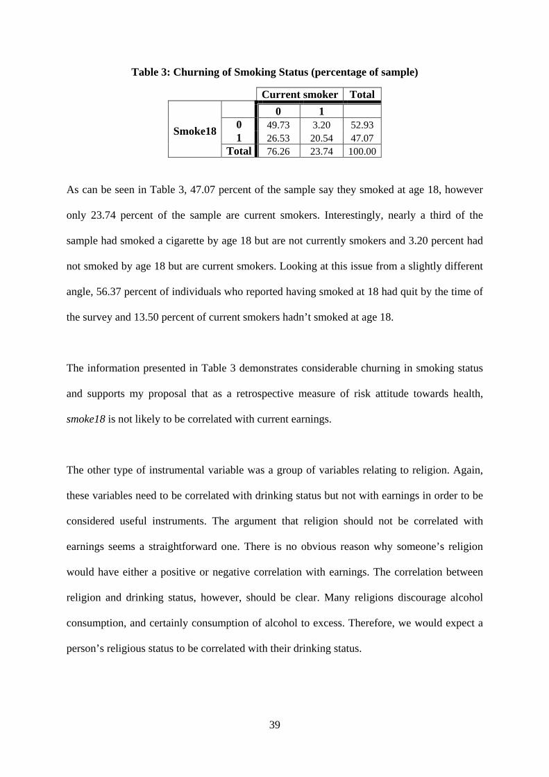
As can be seen in Table 3, 47.07 percent of the sample say they smoked at age 18, however
only 23.74 percent of the sample are current smokers. Interestingly, nearly a third of the
sample had smoked a cigarette by age 18 but are not currently smokers and 3.20 percent had
not smoked by age 18 but are current smokers. Looking at this issue from a slightly different
angle, 56.37 percent of individuals who reported having smoked at 18 had quit by the time of
the survey and 13.50 percent of current smokers hadn’t smoked at age 18.
The information presented in Table 3 demonstrates considerable churning in smoking status
and supports my proposal that as a retrospective measure of risk attitude towards health,
smoke18 is not likely to be correlated with current earnings.
The other type of instrumental variable was a group of variables relating to religion. Again,
these variables need to be correlated with drinking status but not with earnings in order to be
considered useful instruments. The argument that religion should not be correlated with
earnings seems a straightforward one. There is no obvious reason why someone’s religion
would have either a positive or negative correlation with earnings. The correlation between
religion and drinking status, however, should be clear. Many religions discourage alcohol
consumption, and certainly consumption of alcohol to excess. Therefore, we would expect a
person’s religious status to be correlated with their drinking status.

40
Hamilton & Hamilton (1997) used religion variables as instrumental variables in their
research on the same issue. They used a dummy variable indicating whether someone has no
religion, another indicating whether someone attends religious services at least once a month
and also an interaction between this religion attendance variable and a dummy variable
indicating whether an individual’s religion is Catholicism. The rationale behind this
interaction variable is that the Catholic Church has potentially less stringent attitudes towards
drinking than other Christian denominations (Hamilton & Hamilton, 1997, p. 143).
Clearly though, in addition to this potential Catholic interaction effect, the impact of religion
on drinking status may be a complex one and these few variables may not be able to
adequately model the different aspects through which religion could be correlated with
drinking status. Fortunately, HILDA contains very rich information about religion and so it is
possible to model the different transmission mechanisms through which religion may affect
drinking status. The variables that allow this complexity of influence in my model are
Religion-broad (which allows individuals to tick a box representing their religion), frequency
of attendance at religious services and importance of religion. These are questions B26, B27
and B28 of the Self-Completion Questionnaire, and their exact wording can be found in
Appendix 3.
The Religion-broad variable as aggregated in the original HILDA data included 26 different
religion categories, many of which were different denominations of the Protestant Church.
Furthermore, many of categories had very few observations in the sample and when the
drinking status regression was estimated with all 26 variables, a large number of parameters
could not be identified. In order to save degrees of freedom and to avoid this problem, the

41
categories were aggregated to five different groups. The precise definition of each variable
can be found in Appendix 4.
The final group of religion variables used as instrumental variables included dummies for the
different religion categories, a dummy indicating whether the individual attends a religious
service at least once a week, a variable indicating the importance of religion on a scale of 1 to
10 and an interaction variable between each religion category and the importance of religion.
For the group of religion category dummies, the variables used are mutually exclusive and
exhaustive. This is the case for all groups of dummy variables used in this thesis.
Table 4 provides the summary statistics for all instrumental variables, by drinking status.
Table 4: Mean Values for Instrumental Variables by Drinking Status1
Variable
Abstainers Moderate Drinkers Heavy Drinkers Religious attendance 0.1736 0.0755 0.0210 Religious importance 4.2145 2.7969 1.9655 Protestant * 0.3176 0.3326 0.3045 Catholic 0.2644 0.2502 0.2418 Other Christian 0.0606 0.0366 0.0222 Other religion 0.1114 0.0548 0.0166 No religion 0.2460 0.3259 0.4150 Protestant*importance * 1.4407 1.0711 0.7560 Catholic*importance 1.2927 1.0607 0.8214 Other Christian*importance 0.3718 0.1932 0.1285 Other religion*importance 0.8587 0.2835 0.0766 No religion*importance 0.2506 0.1884 0.1830 Smoke18 0.3945 0.4385 0.6535 Number of observations 438 1,241 473
Looking at the summary statistics for the instrumental variables, there are some striking
patterns across the different drinker types. For example, heavy drinkers are by far the most
likely to have smoked by age 18, followed by moderate drinkers and abstainers. A similar
trend is evident for having no religion. In contrast, abstainers are most likely to attend weekly 1 The variables marked with * are those dummies excluded in estimation. This notation is maintained throughout this thesis.
42
religious services and to give a higher importance to religion in their lives, followed moderate
drinkers and heavy drinkers. These statistics reflect the expected patterns and also support the
argument that smoke18 will more strongly identify heavy drinkers, while the religion
variables will more strongly identify abstainers.
Alternative instrumental variables have been used by other studies in this area that would not
have been appropriate to this research. For example Hamilton & Hamilton (1997) use alcohol
price variables as instruments. These are province-specific variables (the study was based on
Canadian data) and three separate variables are included for the price of spirits, wine and beer
(given by sales/volume). The ABS does provide a price index for the composite group of
goods, “alcohol and tobacco”, by capital city in Australia. However, a further breakdown of
prices for just alcohol, or for the sub-groups of alcohol such as spirits, wine and beer, was not
easily obtainable. Given that including these price variables as instrumental variables would
have meant excluding the State variables from the selection and log earnings regression and
that variation in this variable would have been limited by Australia’s eight States and
Territories, it was decided not to pursue these as instrumental variables for my research.
Barrett (2002, p. 84) also used two instrumental variables indicating the proportion of sample
members in an individual’s local area (excluding the individual) who were abstainers and
who were heavy drinkers. These variables were used to identify the ‘wetness’ of the local
social environment and hence its influence on the individual’s drinking behaviour. As
HILDA did not include data about the sample members’ specific geographic location, it was
not possible to use such an instrumental variable in my research.

43
6.5 Independent variables
The independent variables in the earnings regressions are those that make up the vector of
human capital, socioeconomic and job-specific characteristics. They include variables for
age, marital status, country of birth, State of residence, section of State, education, occupation
and sector of employment. A list of the complete definitions of all independent and
instrumental variables can be found in Appendix 4. Summary statistics of the independent
variables included in the log earnings regressions are presented in Table 5.
There are a few notable demographic patterns evident from these summary statistics. The first
of these is the life-cycle pattern of drinking status. Younger workers make up a higher
proportion of heavy drinkers than they do for abstainers or moderate drinkers. Abstainers
seem to be concentrated around those who are middle-aged and moderate drinkers are fairly
smoothly spread across age groups, with a slight skew towards younger individuals.
Compared to the other drinker types, heavy drinkers are more likely to live regionally or
remotely. The moderate drinker group has the highest proportion of individuals with an
undergraduate degree and heavy drinkers have the highest proportion of individuals who did
not complete High School. In terms of work characteristics, moderate drinkers have slightly
higher proportions of professionals, managers and individuals employed in the public sector
while heavy drinkers have slightly higher proportions of individuals working as technicians
or in trades and as labourers.

44
Table 5: Mean Values for Independent Variables by Drinking Status
Variable Abstainers Moderate Drinkers Heavy Drinkers Age 25-29 0.1259 0.1234 0.1726 Age 30-34 0.1338 0.1638 0.1867 Age 35-39 0.1698 0.1551 0.1351 Age 40-44* 0.1852 0.1432 0.1728 Age 45-49 0.1660 0.1594 0.1368 Age 50-59 0.1139 0.1549 0.1138 Age 60-64 0.1053 0.1001 0.0822 Married* 0.6928 0.7889 0.7120 Single 0.3072 0.2111 0.2880 Australian-born* 0.6663 0.7763 0.8481 Immigrant English-speaking 0.0749 0.1101 0.1011 Immigrant other 0.2588 0.1136 0.0507 NSW* 0.3804 0.2888 0.2991 VIC 0.2381 0.2675 0.2604 QLD 0.1740 0.2066 0.2093 SA 0.0518 0.0793 0.0737 WA 0.1195 0.1008 0.1020 TAS 0.0144 0.0255 0.0275 NT 0.0029 0.0060 0.0242 ACT 0.0189 0.0254 0.0038 City* 0.7697 0.7186 0.5835 Regional 0.2204 0.2650 0.3856 Remote 0.0099 0.0164 0.0309 Postgraduate degree 0.0306 0.0754 0.0251 Undergraduate 0.1940 0.2625 0.1577 Diploma* 0.4524 0.4197 0.4364 Year 12 0.1280 0.1174 0.1271 Did not complete High School 0.1950 0.1250 0.2537 Managers 0.1174 0.1881 0.1258 Professionals* 0.1959 0.2701 0.1760 Technicians & Trades 0.2032 0.2122 0.2579 Community & Personal Services 0.0923 0.0517 0.0546 Clerical & Administrative 0.1180 0.0929 0.0871 Sales 0.0482 0.0401 0.0368 Machinery operators 0.1301 0.0871 0.1554 Labourers 0.0949 0.0578 0.1065 Public sector 0.1898 0.2217 0.1808 Number of observations 438 1,241 473

45
7. STATISTICAL ANALYSIS
7.1 Results using OLS and drinking status dummies
A log earnings regression was estimated by OLS, which included the dummy variables
abstainers and heavy drinkers, with moderate drinkers as the excluded variable. This
regression also controlled for human capital, socioeconomic and job characteristics and the
results are presented in Table 6. These results imply that after controlling for the above
characteristics, abstainers receive a wage penalty relative to moderate drinkers and that the
effect on earnings of being a heavy drinker, relative to being a moderate drinker, is unclear.
The estimated coefficient for the abstainer variable is statistically significant at the 1 percent
level and is also economically significant, indicating that abstainers earn 12.16 percent less,
on average, than do moderate drinkers. The estimated coefficient for the heavy drinker
dummy variable is neither statistically nor economically significant.
The results for the abstainer coefficient reflect the pattern of differences in mean ln earnings
of the different drinker types found in Table 1. They also reflect a priori expectations that
moderate drinkers may earn more than abstainers as a result of health and social networking
effects. These results imply that after controlling for other characteristics, the average
difference in log earnings between moderate drinkers and abstainers is actually higher than
that observed in the raw data, which shows that abstainers earn 2.74 percent less than
moderate drinkers, on average.
Furthermore, the expected negative earnings penalty for heavy drinkers, is not observed in
these results. These results may reflect biases arising from the suspected endogeneity
problem and, as such, support the proposed use of a Heckman selection model.

46
Table 6: OLS Regression Results using Drinking Status Dummies2
Variable
Coefficient (Standard Error)
Constant 7.2756*** (0.0558) Abstainers -0.1216*** (0.0338) Heavy Drinkers 0.0034 (0.0274) Age 25-29 -0.1756*** (0.0532) Age 30-34 -0.0597 (0.0432) Age 35-39 -0.0590 (0.0499) Age 45-49 -0.0275 (0.0447) Age 50-59 -0.1102** (0.0523) Age 60-64 -0.0181 (0.0555) Single -0.1423*** (0.0344) Immigrant English-speaking 0.0174 (0.0366) Immigrant other -0.0733 (0.0457) VIC -0.0151 (0.0337) QLD 0.0126 (0.0369) SA -0.0938** (0.0420) WA 0.0933**(0.0459) TAS -0.0865 (0.0544) NT -0.0014 (0.1207) ACT 0.0326 (0.0621) Regional -0.0533** (0.0268) Remote -0.0816 (0.1031) Postgraduate degree 0.2794*** (0.0511) Undergraduate 0.1277*** (0.0363) Year 12 -0.0346 (0.0369) Did not complete High School -0.1712*** (0.0399) Managers 0.0359 (0.0398) Technicians & Trades -0.1680*** (0.0416) Community & Personal Services -0.1188** (0.0470) Clerical & Administrative -0.1391*** (0.0412) Sales -0.2623*** (0.0635) Machinery operators -0.1057** (0.0482) Labourers -0.2963*** (0.0781) Public sector 0.0187 (0.0252) Number of observations 2152 R-squared 0.2042
2 Where *** indicates statistical significance at the 1 percent level, ** indicates statistical significance at the 5 percent level and * indicates statistical significance at the 10 percent level. This system of notation is maintained throughout the rest of this thesis.

47
7.2 Estimation using the Heckman selection model
7.2.1 Results of the selection regression
The first step in this model was to estimate the selection equation, where drinking status is
the dependent variable. The results for this regression and the marginal effects calculated
from these estimates are presented in Table 7. These results offer some interesting insights
about the relevance of the chosen instrumental variables and the effects of socioeconomic and
demographic characteristics on drinking status.
The smoke18 instrumental variable is clearly relevant to the choice of drinking status. It is
statistically significant at the 1 percent level for the heavy drinker outcome and is statistically
significant at the 10 percent level for the abstainer outcome. A likelihood ratio test was also
performed, where the null hypothesis is that the smoke18 variable has no effect on the choice
of drinking status. The value of the likelihood ratio test statistic is 47.53 and is chi-squared
distributed with two degrees of freedom. This test statistic has a p-value of 0.0000 and, as
such, the null hypothesis is decisively rejected.
As well as being statistically significant, the smoke18 variable is economically significant.
While its effect on the probability of being a moderate drinker is small, it has a large effect on
the probability of being either an abstainer or heavy drinker. The results indicate that
someone who had smoked a full cigarette by age 18 is 10.62 percent less likely to be an
abstainer now and is 13.55 percent more likely to be a heavy drinker now. This is the
expected effect and reflects the nature of smoke18 being an indicator for attitudes towards
risky health behaviour.

48
Table 7: Results of Multinomial Logit Selection Equation3
Variable
Abstainers Heavy Drinkers Marginal effects on probabilities4
Coefficient (Standard Error)
Coefficient
(Standard Error) Abstainer Moderate Drinker
Heavy Drinker
Predicted Probability Constant -0.8363** (0.3256) -1.4144*** (0.3390) 0.2363 0.5913 0.1725 Marginal Effect Age 25-29 -0.4570* (0.2744) 0.2470 (0.2361) -0.0839 0.0276 0.0563 Age 30-34 -0.5214** (0.2510) 0.1403 (0.2288) -0.0900 0.0490 0.0410 Age 35-39 -0.1340 (0.2402) -0.1947 (0.2288) -0.0164 0.0381 -0.0217 Age 45-49 -0.4002 (0.2570) -0.3123 (0.2233) -0.0568 0.0851 -0.0284 Age 50-59 -0.6134*** (0.2377) -0.3422 (0.2495) -0.0877 0.1139 -0.0262 Age 60-64 -0.2367 (0.3111) -0.3565 (0.2686) -0.0286 0.0673 -0.0387 Single 0.4600** (0.1887) 0.3694** (0.1562) 0.0699 -0.1034 0.0335 Immigrant English-speaking -0.2765 (0.2283) -0.0680 (0.2205) -0.0446 0.0439 0.0007 Immigrant other 0.6978*** (0.2410) -0.6191** (0.3150) 0.1678 -0.0688 -0.0990 VIC -0.2453 (0.1966) 0.0039 (0.1808) -0.0430 0.0328 0.0102 QLD -0.2874 (0.2234) -0.2835 (0.1829) -0.0395 0.0678 -0.0282 SA -0.5564** (0.2759) -0.2868 (0.2668) -0.0796 0.1005 -0.0209 WA 0.1619 (0.2548) -0.1074 (0.2485) 0.0347 -0.0134 -0.0213 TAS -0.5295 (0.4288) -0.4483 (0.3721) -0.0711 0.1125 -0.0415 NT -0.8401 (0.8183) 1.0211* (0.5414) -0.1501 -0.0851 0.2352 ACT 0.0166 (0.4457) -1.4108** (0.6132) 0.0395 0.0875 -0.1270 Regional -0.1489 (0.1730) 0.4100*** (0.1434) -0.0435 -0.0253 0.0687 Remote -0.2991 (0.5361) 0.6446 (0.4209) -0.0764 -0.0503 0.1268 Postgraduate degree -1.2352*** (0.3757) -0.5199 (0.3636) -0.1520 0.1887 -0.0368 Undergraduate -0.5081** (0.2189) -0.2721 (0.2091) -0.0758 0.0953 -0.0195 Year 12 0.0401 (0.2464) -0.0170 (0.2259) 0.0080 -0.0039 -0.0041 Did not complete High School 0.2882 (0.2169) 0.5066*** (0.1816) 0.0292 -0.0944 0.0652 Managers -0.1804 (0.2645) -0.2297 (0.2278) -0.0232 0.0479 -0.0247 Technicians & Trades 0.0695 (0.2432) 0.1264 (0.2266) 0.0073 -0.0228 0.0155 Community & Personal Services 0.7990** (0.3666) -0.0143 (0.3584) 0.1689 -0.1292 -0.0397 Clerical & Administrative 0.3798 (0.3007) 0.0517 (0.2838) 0.0714 -0.0617 -0.0097 Sales 0.3537 (0.3388) -0.1380 (0.4224) 0.0754 -0.0422 -0.0332 Machinery operators 0.6034** (0.2795) 0.2363 (0.2751) 0.1090 -0.1137 0.0048 Labourers 0.4413 (0.3076) 0.2514 (0.3045) 0.0741 -0.0899 0.0158 Public sector -0.0520 (0.1999) -0.0638 (0.1867) -0.0068 0.0137 -0.0069 Religious attendance 0.6581** (0.2717) -0.8472* (0.5078) 0.1679 -0.0543 -0.1136 Religious importance 0.0946** (0.0394) -0.0209 (0.0423) 0.0179 -0.0111 -0.0068 Catholic 0.1889 (0.3401) 0.1334 (0.2666) 0.0291 -0.0403 0.0112 Other Christian 0.4631 (0.7027) -1.1739 (0.7422) 0.1318 -0.0068 -0.1250 Other religion -0.4705 (0.7135) -1.1927* (0.6848) -0.0484 0.1599 -0.1115 No religion 0.0418 (0.2444) 0.2517 (0.1880) -0.0031 -0.0321 0.0352 Catholic*importance -0.0698 (0.0606) -0.0056 (0.0639) -0.0124 0.0103 0.0020 Other Christian*importance -0.0603 (0.0974) 0.1687 (0.1157) -0.0178 -0.0088 0.0265 Other religion*importance 0.0917 (0.1032) 0.1238 (0.1227) 0.0115 -0.0254 0.0139 No religion*importance 0.0905 (0.0848) -0.0438 (0.0922) 0.0181 -0.0082 -0.0099 Smoke18 -0.2761* (0.1626) 0.7041*** (0.1405) -0.0782 -0.0354 0.1136 Number of observations 2152 Log-likelihood -1919.3337
3 Moderate drinkers are the base group for this estimation and for all subsequent multinomial logit estimations 4 Marginal effects are calculated at the mean levels of the independent variables. For dummy variables they represents the discrete change in log earnings as the dummy is switched on from 0 to 1. This is the same for all subsequent marginal effects calculations.

49
Several of the religion variables are individually statistically significant and the group of
religion variables are jointly highly significant. They also have the expected effects.
Religious attendance and religious importance are statistically significant at the 1 percent
level for the abstainer outcome. Religious attendance is also statistically significant at the 10
percent level for the heavy drinker outcome. Again, a likelihood ratio test was performed,
where the null hypothesis is that the entire group of “religion” variables has no effect on the
choice of drinking status. The likelihood ratio test statistic has a value of 100.50 and is chi-
squared distributed with 20 degrees of freedom. Again, the null hypothesis is decisively
rejected and the results show that the group of religion variables are highly relevant to the
selection of drinking status.
The independent variables present a range of interesting results. The group of age dummies
compares the effect of age on the selection of drinking status relative to the excluded group,
those aged 40 to 44. While the coefficients are imprecisely estimated, the results suggest that
younger individuals are more likely to be heavy drinkers and that the older the individual, the
more likely they are to be a moderate drinker. This life-cycle trend in drinking status reflects
the expected trend and also the summary statistics presented in Section 6.5.
The education dummies also reveal some clear socioeconomic trends in the choice of
drinking status. The excluded variable in this group is diploma, representing those with a
post-secondary diploma or certificate. The estimated coefficient for the postgraduate and
undergraduate variables are statistically significant at the 1 percent and 5 percent levels,
respectively, for the abstainer outcome. The estimated coefficient for the variable did not
complete High School, is statistically significant at the 1 percent level for heavy drinkers. The
accompanying marginal effects suggest that those with a postgraduate degree are 15.20

50
percent less likely to be abstainers and 18.87 percent more likely to be moderate drinkers than
those with a post-secondary diploma. The effect on being a heavy drinker is not large. The
effect of holding an undergraduate degree is similar but of a lesser magnitude, with this group
7.58 percent less likely to be abstainers and 9.53 percent more likely to be moderate drinkers.
At the other end of the education scale, those who did not complete high school are 9.44
percent less likely to be moderate drinkers and 6.52 percent more likely to be heavy drinkers
than those with a post-secondary diploma. These results demonstrate a clear relationship
between the level of education of male workers and their resulting drinking behaviour.
It seems that marriage also moderates drinking behaviour. The single variable is statistically
significant at the 5 percent level for both the abstainer and heavy drinker outcome and the
marginal effect suggests that single male workers are 10.34 percent less likely to be moderate
drinkers than those who are married. Other demographic patterns are suggested by the results
of the selection regression. Immigrants from non-English speaking countries are 16.78
percent more likely to be abstainers and 9.90 percent less likely to be heavy drinkers than
individuals born in Australia, where the estimated coefficients for the immigrant other
dummy is statistically significant at 1 percent and 5 percent levels for the abstainer and heavy
drinker outcomes respectively. Geography also seems to play an important role in choice of
drinking status. The marginal effect for the regional dummy suggests that, relative to those
individuals living in cities, male workers living regionally are 6.87 percent more likely to be
heavy drinkers and the remote dummy suggests those who live remotely are 12.68 percent
more likely to be heavy drinkers.
Finally, several dummy variables indicating occupational status demonstrate economically
significant marginal effects of their occupation on the choice of drinking status. Relative to

51
the base group, professionals, individuals in almost all occupations (excluding managers) are
more likely to be abstainers and less likely to be moderate drinkers. This trend suggests that
the type of occupation you are employed in is important in determining drinking status choice
and that those individuals in high-powered jobs, professionals and managers, are more likely
to drink alcohol than individuals in other occupations.
Given that both the independent and instrumental variables appear to affect drinking status in
the expected way and that the instrumental variables are statistically relevant to the selection
regression, these estimates can be used for the construction of the IMR used in the log
earnings regressions.
7.2.2 Results for log earnings equations
The second step of the Heckman selection model was to estimate the log earnings regressions
for each drinker type, the results of which are presented in Table 8. Most of the coefficients
are statistically significant for the moderate drinker regression, while this is the case for fewer
variables as part of the abstainer and heavy drinker regressions. This result is most likely due
to the fact that the sample size for the moderate drinker regression is nearly three times larger
for this group than for the other groups. However, most estimated coefficients in all three
regressions have economic significance.
For example, the postgraduate degree dummy variable indicates an earnings premium of
roughly 25 percent, relative to having a post-secondary diploma or certificate, for all three
drinker types. However, this result is imprecisely estimated for both abstainers and heavy
drinkers, where the standard errors are at least half the size of the estimated coefficient.
Interestingly though, the returns to this education characteristic demonstrate the expected

52
pattern, where moderate drinkers have the highest returns to postgraduate qualifications,
followed by abstainers, followed by heavy drinkers.
The education earnings premium demonstrated by the estimates for the postgraduate degree
variable is also evident for the undergraduate variable across all drinker types. This premium
is smaller than that for a postgraduate degree, but demonstrates the same pattern in returns to
drinking status. For those who did not complete high school, the earnings penalty is
statistically significant for both abstainers and heavy drinkers and suggests the penalty is
highest for abstainers, followed by heavy drinkers, followed by moderate drinkers.
As with the with the education dummies, by comparing the estimated coefficients of other
variables it is possible to gain a sense of how the returns to human capital, socioeconomic
and job characteristics vary amongst the three different groups. For instance, by looking at
the constant it appears as though, for the base group5
While imprecisely estimated for abstainers and heavy drinkers, the age-earnings profile of
each drinker group roughly reflects the expected trend, and that found by both Barrett (2002)
and Hamilton & Hamilton (1997). The expected result is that the age-earnings profile will
have a roughly concave shape. This profile is precisely estimated for moderate drinkers and
the expected concave shape is clear in the results, with the base group, those aged 40 to 44,
gaining the highest predicted average earnings. This profile is less apparent for abstainers,
where the concave profile disappears for the predictions for those aged 35 to 39 and 45 to 49,
for whom the estimations are imprecise, and for those aged 60 to 64 for whom there appears
to be an earnings premium. The concave age-earnings profile disappears almost entirely for
at least, a moderate drinker earns, on
average, more than a heavy drinker, who will earn more, on average, than an abstainer.
5 A male worker aged 40-44, with a post-secondary diploma or certificate, who is married, lives in a city in NSW, is Australian born and works in the private sector as a professional.

53
heavy drinkers, for whom the estimated coefficients on all the age dummy variables are both
statistically and economically insignificant.
Table 8: Results of Log Earnings Regression by Drinking Status
Variable Abstainers Moderate Drinkers Heavy Drinkers Coefficient
(Standard Error) Coefficient
(Standard Error) Coefficient
(Standard Error) Constant 6.8401*** (0.2091) 7.4597*** (0.1327) 7.4213*** (0.1685) IMR 0.1651* (0.0922) -0.1557 (0.1651) -0.0818 (0.1048) Age 25-29 -0.0627 (0.1327) -0.3598*** (0.0531) -0.0235 (0.0795) Age 30-34 -0.1489 (0.0984) -0.1048** (0.0504) 0.0010 (0.0745) Age 35-39 0.0062 (0.1207) -0.1395*** (0.0513) -0.0544 (0.0810) Age 45-49 0.0343 (0.1233) -0.1049** (0.0497) 0.0074 (0.0783) Age 50-59 -0.1040 (0.1127) -0.2408*** (0.0718) 0.0748 (0.0929) Age 60-64 0.1192 (0.1410) -0.1705*** (0.0585) 0.0986 (0.0958) Single -0.1385** (0.0692) -0.1021** (0.0467) -0.1007** (0.0458) Immigrant English-speaking 0.0308 (0.0707) -0.0188 (0.0484) 0.0167 (0.0834) Immigrant other 0.1200 (0.1129) -0.1191* (0.0630) -0.0551 (0.0844) VIC 0.0770 (0.0896) -0.0570 (0.0420) -0.0704 (0.0569) QLD 0.1392 (0.0982) -0.0711 (0.0442) 0.0097 (0.0623) SA -0.0093 (0.1209) -0.1317*** (0.0493) -0.1959** (0.0870) WA 0.1221 (0.1128) 0.0676 (0.0544) 0.0929 (0.0841) TAS -0.0979 (0.1506) -0.1638** (0.0801) 0.0090 (0.0994) NT -0.0950 (0.1891) 0.0641 (0.2219) -0.0641 (0.1744) ACT 0.2140 (0.1572) -0.0901 (0.0736) 0.2574 (0.2197) Regional -0.0032 (0.0730) -0.0771** (0.0339) -0.0921 (0.0565) Remote -0.1313 (0.1819) -0.1270 (0.1486) -0.0588 (0.1859) Postgraduate degree 0.2480 (0.1581) 0.2770*** (0.0773) 0.2409** (0.1225) Undergraduate 0.0886 (0.0839) 0.1538*** (0.0536) 0.0208 (0.0720) Year 12 -0.0328 (0.0704) -0.0102 (0.0504) -0.0930 (0.0823) Did not complete High School -0.2737*** (0.0978) -0.0797 (0.0511) -0.1487*** (0.0559) Manager 0.0300 (0.1133) 0.0543 (0.0473) -0.0489 (0.0856) Technicians & Trades -0.1863 (0.1168) -0.0831 (0.0547) -0.3002*** (0.0793) Community & Personal Services -0.0519 (0.1083) -0.1226* (0.0726) -0.1493 (0.1045) Clerical & Administrative -0.1735 (0.1102) -0.1043** (0.0531) -0.1273 (0.0844) Sales worker -0.1383 (0.1365) -0.3242*** (0.0833) -0.1933 (0.1266) Machinery operator -0.0648 (0.1083) -0.0166 (0.0729) -0.2872*** (0.0908) Labourer -0.4270** (0.1902) -0.1406** (0.0701) -0.3046*** (0.0942) Public sector 0.0453 (0.0572) 0.0099 (0.0318) 0.0142 (0.0546) Number of observations 438 1241 473 R-squared 0.2685 0.2087 0.1734
Finally, looking at the estimated coefficients for some of the occupation dummy variables, it
seems as though the earnings returns may differ substantially between drinker types. For
example, for the labourer variable there is an earnings penalty, relative to working as a
professional, across all three drinker types that is also statistically significant for all three
drinker types at at least the 5 percent level. However, this penalty is twice as large for heavy

54
drinkers as it is for moderate drinkers and is half as large again for abstainers. Another
example is for the machinery operator dummy, for which the earnings penalty relative to
professionals is by far the largest for heavy drinkers. This may reflect that job performance as
a machinery operator or driver is severely affected by the consumption of alcohol and that
there may be testing regimes at some workplaces where the impact of alcohol consumption
on job performance would be a critical health and safety issue.
Clearly, by simply examining the differences between the estimated coefficients of each
drinker type, it is very difficult to determine the overall pattern in how returns to
characteristics differ between the three groups. As such, it is instructive to look at the
earnings decompositions, presented in the section 7.3.
Looking now at the IMR for each log earnings regression, the estimated coefficient is only
statistically significant for the abstainers regression and even then, only at the 10 percent
level. These imprecise estimates potentially indicate that sample selection bias is not present,
as the null hypothesis that there is no correlation between the unobservables in the selection
equation and the log earnings equation cannot be rejected. However this result does not
necessarily indicate that the IMR is not important and this issue is further investigated as part
of the sensitivity analysis in Section 7.5.
The magnitudes of the estimated coefficient for the IMRs are economically significant for
each drinking status log earnings regression. For the non-drinker and heavy drinker groups,
the suggested signs of the coefficients on the IMRs do reflect the hypothesised sample
selection effect. The negative estimated coefficient for the heavy drinker IMR indicates
positive self-selection may exist. This result indicates that if a randomly selected person were
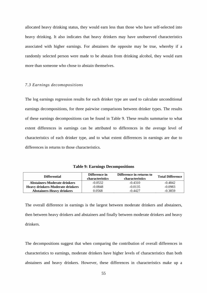
55
allocated heavy drinking status, they would earn less than those who have self-selected into
heavy drinking. It also indicates that heavy drinkers may have unobserved characteristics
associated with higher earnings. For abstainers the opposite may be true, whereby if a
randomly selected person were made to be abstain from drinking alcohol, they would earn
more than someone who chose to abstain themselves.
7.3 Earnings decomopositions
The log earnings regression results for each drinker type are used to calculate unconditional
earnings decompositions, for three pairwise comparisons between drinker types. The results
of these earnings decompositions can be found in Table 9. These results summarise to what
extent differences in earnings can be attributed to differences in the average level of
characteristics of each drinker type, and to what extent differences in earnings are due to
differences in returns to those characteristics.
Table 9: Earnings Decompositions
Differential Difference in characteristics
Difference in returns to characteristics Total Difference
Abstainers-Moderate drinkers -0.0532 -0.4310 -0.4842 Heavy drinkers-Moderate drinkers -0.0848 -0.0135 -0.0983
Abstainers-Heavy drinkers 0.0568 -0.4427 -0.3859
The overall difference in earnings is the largest between moderate drinkers and abstainers,
then between heavy drinkers and abstainers and finally between moderate drinkers and heavy
drinkers.
The decompositions suggest that when comparing the contribution of overall differences in
characteristics to earnings, moderate drinkers have higher levels of characteristics than both
abstainers and heavy drinkers. However, these differences in characteristics make up a

56
relatively small part of the overall differences in earnings. When comparing heavy drinkers
and abstainers, it is abstainers who appear to have higher overall levels of observable
characteristics.
However, the more interesting aspect of the earnings decompositions is to compare the
difference in returns to the average levels of characteristics between drinker types. The results
suggest that the overall returns to observable characteristics are highest for moderate
drinkers, followed by heavy drinkers, then by abstainers. However, the difference in returns
to characteristics between moderate and heavy drinkers appears to be quite small and the
main source of lower earnings from heavy drinking appears to arise from differences in levels
of characteristics. This indicates that heavy drinking, relative to moderate drinking, does not
have much effect on productivity returns.
The biggest difference between drinker types looks to be that associated with the returns to
characteristics between moderate drinkers and abstainers. Moderate drinkers, on average,
have substantially larger returns to observable characteristics than do abstainers. This result
supports the hypothesis that moderate drinkers attract productivity benefits through both
health and social networking effects. The sensitivity of these results to changes in the
definitions of drinking status will be explored in section 7.5.3.
7.4 Sensitivity analysis of the Heckman selection estimation
The initial results presented in section 7.2 point towards three main areas where an analysis
of the sensitivity of results is important. The first of these is to see how the assumption of
exogenous selection affects results, by estimating the log earnings regressions without the
IMRs. Secondly, given the strong apparent effect of religious attendance on drinking status

57
choice in the selection regression relative to the other religion variables, an argument could
be made that religious attendance is endogenous to drinking status through possible reverse
causality. Finally, the sensitivity of the results to alternative demarcations between drinking
status definitions will be explored.
7.4.1 Exogenous selection
The three log earnings regressions were estimated assuming exogeneity of sample selection
by estimating them without the IMR. The results for these regressions can be found in
Appendix 9 and can be compared to the original estimations presented in Table 8. These
results are qualitatively similar across all drinker types when compared with the original
estimations. All estimated coefficients maintain the same sign are estimated with a similar
magnitude.
However, there are some variables for which the estimated coefficients change slightly in
magnitude when estimated under exogenous selection. For example, the constant terms
among the three different drinker type are much closer in size under exogenous sampling than
when they are estimated using the Heckman selection model. This movement is in the
direction expected for each drinking status now that selection bias is not being controlled for.
So, for example the constant increases for abstainers now that the estimates are not corrected
for negative self-selection. For moderate and heavy drinkers, the constants decrease now that
the estimates are not corrected for positive self-selection. These changes imply that the results
are sensitive to the inclusion of the IMR. The implication is that the inclusion of the IMR is
important in correcting for self-selection bias. Hence, in spite of the imprecise estimates of
the IMRs in section 7.2.2, they still constitute an important component of the estimates.

58
7.4.2 Exclusion of religious attendance
In order to determine whether the results are sensitive to the inclusion of religious attendance
as part of the group of religion instrumental variables, the Heckman selection model was
estimated excluding this variable in the selection equation. The rationale for this is that
religious attendance is potentially endogenous to drinking status choice. This endogeneity
problem might occur if people select their religious attendance based upon their drinking
status. For instance, those who have a religious background and may otherwise be practicing
might not actually attend religious services if their preference is to drink moderately or
heavily. It is not instantly clear whether this reverse causality may be a problem, hence the
second part of the sensitivity analysis is to see whether the results are sensitive to the
inclusion of the religious attendance variable.
The results for selection equation are presented in Table 10 and the results for the log
earnings regressions are presented in Appendix 6. These can be compared to the original
results presented in Tables 7 and 8.
A quick look at the marginal effects and estimated coefficients shows that the results are
qualitatively similar to those obtained when religious attendance was included. None of the
estimated coefficients change sign and all of them stay within a similar magnitude. However,
the estimated coefficients do seem to have moved around slightly for some variables. Perhaps
the only notable change is that the religious importance coefficient for the abstainer outcome
has increased nearly 50 percent in magnitude, from 0.0946 to 0.1402 and from having
statistical significance at the 5 percent level to having statistical significance at the 1 percent
level. This change suggests that religious importance may be capturing some of the effects of
religious attendance under this specification.
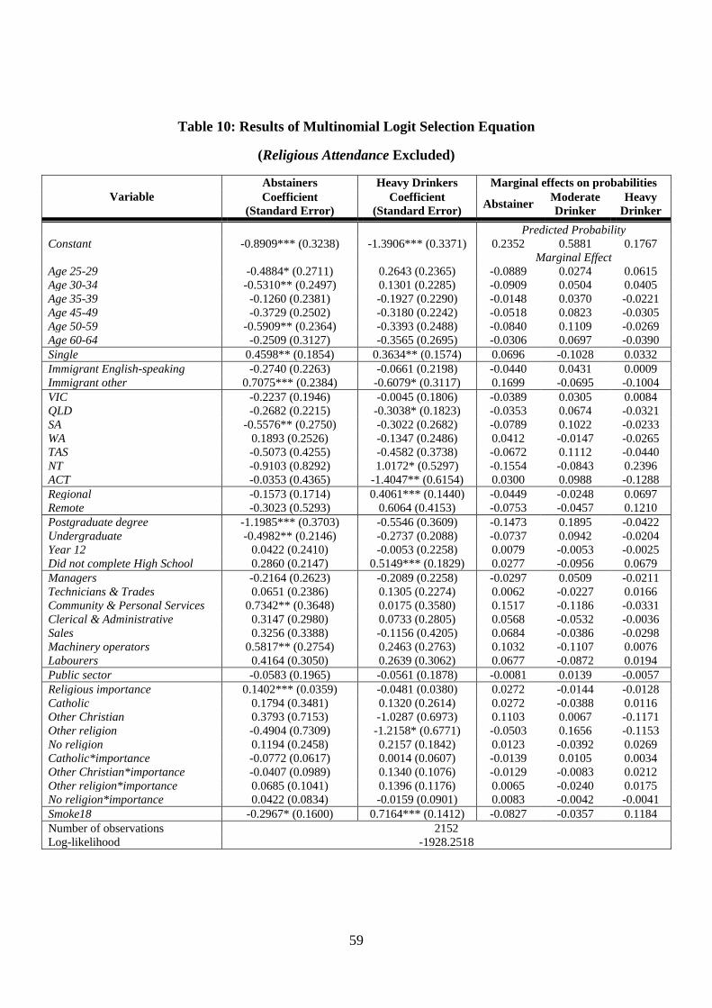
59
Table 10: Results of Multinomial Logit Selection Equation
(Religious Attendance Excluded)
Variable Abstainers Heavy Drinkers Marginal effects on probabilities Coefficient
(Standard Error) Coefficient
(Standard Error) Abstainer Moderate Drinker
Heavy Drinker
Predicted Probability Constant -0.8909*** (0.3238) -1.3906*** (0.3371) 0.2352 0.5881 0.1767
Marginal Effect Age 25-29 -0.4884* (0.2711) 0.2643 (0.2365) -0.0889 0.0274 0.0615 Age 30-34 -0.5310** (0.2497) 0.1301 (0.2285) -0.0909 0.0504 0.0405 Age 35-39 -0.1260 (0.2381) -0.1927 (0.2290) -0.0148 0.0370 -0.0221 Age 45-49 -0.3729 (0.2502) -0.3180 (0.2242) -0.0518 0.0823 -0.0305 Age 50-59 -0.5909** (0.2364) -0.3393 (0.2488) -0.0840 0.1109 -0.0269 Age 60-64 -0.2509 (0.3127) -0.3565 (0.2695) -0.0306 0.0697 -0.0390 Single 0.4598** (0.1854) 0.3634** (0.1574) 0.0696 -0.1028 0.0332 Immigrant English-speaking -0.2740 (0.2263) -0.0661 (0.2198) -0.0440 0.0431 0.0009 Immigrant other 0.7075*** (0.2384) -0.6079* (0.3117) 0.1699 -0.0695 -0.1004 VIC -0.2237 (0.1946) -0.0045 (0.1806) -0.0389 0.0305 0.0084 QLD -0.2682 (0.2215) -0.3038* (0.1823) -0.0353 0.0674 -0.0321 SA -0.5576** (0.2750) -0.3022 (0.2682) -0.0789 0.1022 -0.0233 WA 0.1893 (0.2526) -0.1347 (0.2486) 0.0412 -0.0147 -0.0265 TAS -0.5073 (0.4255) -0.4582 (0.3738) -0.0672 0.1112 -0.0440 NT -0.9103 (0.8292) 1.0172* (0.5297) -0.1554 -0.0843 0.2396 ACT -0.0353 (0.4365) -1.4047** (0.6154) 0.0300 0.0988 -0.1288 Regional -0.1573 (0.1714) 0.4061*** (0.1440) -0.0449 -0.0248 0.0697 Remote -0.3023 (0.5293) 0.6064 (0.4153) -0.0753 -0.0457 0.1210 Postgraduate degree -1.1985*** (0.3703) -0.5546 (0.3609) -0.1473 0.1895 -0.0422 Undergraduate -0.4982** (0.2146) -0.2737 (0.2088) -0.0737 0.0942 -0.0204 Year 12 0.0422 (0.2410) -0.0053 (0.2258) 0.0079 -0.0053 -0.0025 Did not complete High School 0.2860 (0.2147) 0.5149*** (0.1829) 0.0277 -0.0956 0.0679 Managers -0.2164 (0.2623) -0.2089 (0.2258) -0.0297 0.0509 -0.0211 Technicians & Trades 0.0651 (0.2386) 0.1305 (0.2274) 0.0062 -0.0227 0.0166 Community & Personal Services 0.7342** (0.3648) 0.0175 (0.3580) 0.1517 -0.1186 -0.0331 Clerical & Administrative 0.3147 (0.2980) 0.0733 (0.2805) 0.0568 -0.0532 -0.0036 Sales 0.3256 (0.3388) -0.1156 (0.4205) 0.0684 -0.0386 -0.0298 Machinery operators 0.5817** (0.2754) 0.2463 (0.2763) 0.1032 -0.1107 0.0076 Labourers 0.4164 (0.3050) 0.2639 (0.3062) 0.0677 -0.0872 0.0194 Public sector -0.0583 (0.1965) -0.0561 (0.1878) -0.0081 0.0139 -0.0057 Religious importance 0.1402*** (0.0359) -0.0481 (0.0380) 0.0272 -0.0144 -0.0128 Catholic 0.1794 (0.3481) 0.1320 (0.2614) 0.0272 -0.0388 0.0116 Other Christian 0.3793 (0.7153) -1.0287 (0.6973) 0.1103 0.0067 -0.1171 Other religion -0.4904 (0.7309) -1.2158* (0.6771) -0.0503 0.1656 -0.1153 No religion 0.1194 (0.2458) 0.2157 (0.1842) 0.0123 -0.0392 0.0269 Catholic*importance -0.0772 (0.0617) 0.0014 (0.0607) -0.0139 0.0105 0.0034 Other Christian*importance -0.0407 (0.0989) 0.1340 (0.1076) -0.0129 -0.0083 0.0212 Other religion*importance 0.0685 (0.1041) 0.1396 (0.1176) 0.0065 -0.0240 0.0175 No religion*importance 0.0422 (0.0834) -0.0159 (0.0901) 0.0083 -0.0042 -0.0041 Smoke18 -0.2967* (0.1600) 0.7164*** (0.1412) -0.0827 -0.0357 0.1184 Number of observations 2152 Log-likelihood -1928.2518

60
Looking at the results for the log earnings regressions when religious attendance is excluded
from the selection equation, the estimated coefficients remain very similar for all variables
except the IMR. This result suggests that the unconditional earnings decompositions will
show very similar results to those calculated when religious attendance is included in the
selection equation. However, while the exclusion of religious attendance doesn’t affect the
precision of the IMR estimates, it decreases the magnitude of the estimated coefficients
slightly for abstainers and moderate drinkers and increases it slightly for heavy drinkers. It
was not possible to test explicitly for the endogeneity of religious attendance, without
estimating a selection equation for the choice of religious attendance and finding suitable
instrumental variables. As such, it is inconclusive as to whether this variable is endogenous to
drinking status choice. However, because other coefficient estimates have not been greatly
affected and the IMRs have greater explanatory power when estimations are performed using
it as an instrument, its inclusion is the preferred specification of the model.
7.4.3 Drinking status definition
The results were also estimated under two different definitions of drinking status, one more
strict on safe drinking limits and one more lenient towards safe drinking limits. The former
reflects the current NHMRC (2009) guidelines and the latter reflects the demarcations used in
previous research by Barrett (2002) and Hamilton & Hamilton (1997). The former will
hereby be referred to as the NHMRC definition and the latter as the alternative definition.
Under the 2009 NHMRC guidelines, anything more than two standard drinks per sitting is
considered to be unsafe drinking and, using this definition, over half the sample is classified
as heavy drinkers. Referring back to Table 2, all those who were previously classified as
heavy drinker will still be classified as heavy drinkers. In addition, those individuals who fall

61
in the “3 to 4” or “5 to 6” standard drinks columns and were not already classified as heavy
drinkers, are now classified as heavy drinkers. Under this definition, 52.56 percent of the
sample are defined as heavy drinkers, 26.91 percent as moderate drinkers and 20.53 percent
as abstainers.
Under the demarcations used by Barrett (2002) and Hamilton & Hamilton (1997), an
individual can have up to seven standard drinks in one sitting before being classified as a
heavy drinker. The impact of this change on the proportions of the sample in each category is
less severe. Looking at Table 2, those who were previously classified as heavy drinkers and
who drank 5 to 6 standard drinks either 5 to 6 days per week or everyday are now classified
as moderate drinkers. Similarly, those who were previously classified as heavy drinkers
because they drank more than 6 standard drinks at least weekly, even though they would
otherwise have been considered moderate drinkers, are now classified as moderate drinkers.
The resulting breakdown of the sample using this definition is that 9.52 percent are classified
as heavy drinkers, 65.23 percent are classified as moderate drinkers and 25.25 percent are
classified as abstainers.
The log earnings regressions were again estimated for all three drinker types using the
Heckman selection method. The results of the selection equation and log earnings regressions
for the NHMRC definition can be found in Appendix 7 and for the alternative definition the
results can be found in Appendix 8.
I find that the estimation of the log earnings regressions is sensitive to the definition of the
drinking status groups. The effect on the estimation of the IMR is particularly notable. Under
the NHMRC definition, the estimated coefficients of the IMR become even less precise.

62
While they all maintain the same sign, and for moderate drinkers and heavy drinkers they
stay within the same magnitude, the IMR decreases in magnitude significantly for abstainers.
Conversely, using the alternative definition no further precision is lost and magnitude of the
IMR for abstainers and heavy drinkers increases. This indicates that the self-selection bias
had been amplified under this definition.
Clearly, under the assumptions of this model, these shifts in the demarcations between
different drinker types should have an impact on the estimated returns to observable
characteristics for each group. As the NHMRC definition results in the majority of the sample
being classified as heavy drinkers, it is expected that the differences in returns to
characteristics will not be clear-cut as in the original estimations. Similarly, under the
alternative definition the differences in returns to observable characteristics should be more
stark. Under this definition, it is really only those who consume alcohol in quantities a good
deal greater than the current NIH guidelines who are classified as heavy drinkers and as such,
the relationship found using the NIH definition should be more pronounced under this
definition. As was the case under the original estimation, the best way to get a sense of how
drinking status affects differences in earnings is through earnings decompositions, the results
of which are presented in Table 11. These can be compared to the original earnings
decompositions presented in Table 9.
Under the NHMRC definition, the results appear as though individuals have been randomly
allocated to each group. There is very little difference in earnings overall and the small
difference that does exist is mostly attributable to differences in levels of characteristics,
rather than returns to those characteristics. This finding is in contrast to that found using the
NIH definition of drinking status. These results suggest that using the NHMRC definition for

63
heavy drinking, with a very low threshold of maximum daily consumption, there is no
apparent labour market effect of drinking status. If the NHMRC guidelines are correct from a
health standpoint, the implication is that the threshold for safe drinking levels in a purely
health-related or physiological sense is much lower than that for labour market returns.
Table 11: Earnings Decompositions for Change in Drinking Status Definitions
Differential Difference in characteristics
Difference in returns to characteristics
Total Difference
Abstainers-Moderate drinkers 0.0574 0.0185 0.0759 NHMRC Heavy drinkers-Moderate drinkers -0.0141 0.0218 0.0078
Abstainers-Heavy drinkers 0.0461 0.0002 0.0463 Abstainers-Moderate drinkers 0.1725 -0.6222 -0.4497
Alternative Heavy drinkers-Moderate drinkers 0.1706 -0.2140 -0.0435 Abstainers-Heavy drinkers -0.0061 -0.4002 -0.4062
The earnings decompositions under the alternative definition of drinker types also provides
some interesting results. The total difference in earnings for the three pairwise comparisons
remains roughly unchanged under the alternative definition. However, the breakdown of this
difference between levels of characteristics and returns to those characteristics changes
significantly.
When comparing moderate drinkers to both abstainers and heavy drinkers, the difference in
the average level of characteristics changes from being in favour of moderate drinkers in each
case, to being in favour of abstainers and heavy drinkers. The difference in levels of
characteristics also changes from being slightly in favour of abstainers relative to heavy
drinkers to being roughly equal for those two groups.
The premium received by moderate drinkers relative to abstainers in terms of returns to
observable characteristics increases by nearly 50 percent under the alternative definition. This
premium relative to heavy drinkers also increases dramatically. However, the earnings

64
decompositions still show that heavy drinkers are not penalised in terms of returns to
characteristics relative to abstainers. In fact, they still have much larger returns to observable
characteristics than do abstainers.
This increase in the productivity returns to observable characteristics for moderate drinkers
under this definition suggests that those who were previously classified as heavy drinkers,
should be classified as moderate drinkers from a labour market perspective as they receive
higher productivity returns than those now classified as abstainers or heavy drinkers. The
implication seems to be that there are continued productivity benefits from heavier levels of
drinking, potentially from social networking, even though these levels of drinking may be
damaging to health. This change in demarcation also shows much lower productivity returns
to heavy drinking relative to moderate drinking. The magnitude of the difference increases
more than two-fold. Presumably, at a certain threshold, heavy drinkers will also have lower
productivity returns than abstainers. A potential extension of this sensitivity analysis, given
the findings, might be to vary the threshold of alcohol consumption for heavy drinking to
determine where the largest difference between the productivity returns of moderate and
heavy drinking lies and where heavy drinking is penalised relative to abstention. However, as
the threshold for heavy drinking is increased, the number of individuals left in the heavy
drinker sub-sample will decrease and it will become more difficult to obtain precise
estimates. Hence, it may be necessary to obtain a larger sample in order to perform such an
analysis.

65
8. CONCLUSION
The excessive consumption of alcohol in Australia has come under scrutiny recently. This
attention has been accompanied by public discussion, a large program of Federal government
spending on awareness campaigns and a recent downwards revision of the NHMRC safe
drinking guidelines. While the damaging effects of problem drinking on health and personal
relationships are widely known, there is a growing literature on the economic costs to
individuals of problem drinking or alcohol dependency. Conversely, there has been active
debate in the medical literature for some time now about the potential positive health benefits
of moderate alcohol consumption. Flowing on from the medical literature is also a growing
literature about the potential positive economic effects of moderate alcohol consumption.
This thesis contributes to the economics literature about alcohol consumption and its effect
on earnings in Australia. The focus is on the effect of alcohol consumption on earnings for
those who are already in full-time employment, rather than its effect on the probability of
being employed. Through positive health and social networking effects, moderate alcohol
consumption is thought to have a positive impact on earnings, relative to abstention from
alcohol consumption. However, due to the negative health impacts of excessive drinking, it is
hypothesised that heavy drinkers will receive an earnings penalty relative to both moderate
drinkers and abstainers.
Recent literature in this area tends to find an earnings premium for moderate drinking, which
is reduced for heavy levels of drinking. The literature that focuses only on alcohol
dependency finds a definite earnings penalty for this population. In order to reflect this
hypothesised U-shaped effect of alcohol consumption on personal well-being, three different
categories of drinking status are used to classify individuals as part of this research:

66
abstainers, moderate drinkers and heavy drinkers. These classifications are made according to
the current NIH guidelines to safe drinking levels.
The potential endogeneity of alcohol consumption and earnings is a major problem in the
estimation of this effect. Given the population of interest is those who are already in full-time
work, it is likely that individuals self-select their drinking status. For example, those who are
heavy drinkers and who work full-time may be those individuals in society who are best able
to cope with higher levels of alcohol consumption. They may also be those individuals who
drink as a coping mechanism for the stress of their employment. As such, it is important to
use an econometric model that is able to account for this potential endogeneity problem.
As a result of the categorical nature of drinking status in this research, and in order to cater to
the potential endogeneity problem, my econometric analysis uses an extension of the
Heckman selection model. This requires an estimation of the selection of individuals into
drinking status and the estimation of a separate log earnings regression for abstainers,
moderate drinkers and heavy drinkers. As such, it is possible to compare the average
productivity returns to each drinking status as indicated by the estimated coefficients in each
log earnings regression. By calculating earnings decompositions, it is possible to get an
overall sense of the differences in these returns between drinker types.
My results show that there is an earnings premium for moderate drinkers relative to
abstainers and a small earnings penalty for heavy drinkers relative to moderate drinkers, but
not relative to abstainers. The premium for moderate drinkers relative to abstainers appears to
stem mostly from returns to observable characteristics, rather than differences in the level of
those characteristics. My results also show that there is a very small earnings penalty for

67
heavy drinking relative to moderate drinking, however this stems mostly from differences in
the level of characteristics between the two groups and very little is attributable to differences
in productivity returns. Due to the small size of this penalty, my results suggest that even
heavy drinkers earn a premium relative to abstainers.
These results are sensitive to the definition of drinking status. When the threshold for heavy
drinkers is lowered to the daily consumption levels currently recommended by the NHMRC,
over half the sample is classified as heavy drinkers and the earnings premium for drinking
effectively disappears. This result may be because the sample is effectively randomly divided
into three sub-groups under this definition. However, when the safe drinking threshold is
increased, relative to the original definition, the differences in productivity returns that were
found using the original estimations become more stark. Moderate drinkers have even higher
returns to observable characteristics relative to abstainers and heavy drinkers have much
lower returns relative to moderate drinkers. However, heavy drinkers still do have higher
productivity returns than do abstainers.
This shift suggests that those individuals previously classified as heavy drinkers, but who
were at the lower end of alcohol consumption of this group, were actually receiving relatively
high productivity returns. As such, from a health perspective they would be classified as
heavy drinkers, but in terms of the economic benefits they should be classified as moderate
drinkers. This finding suggests that it would be possible to adjust the threshold between
moderate and heavy drinking in order to determine at what stage the greatest difference
between the productivity returns of moderate and heavy drinking occurs. Presumably, at
some point, the returns to heavy drinking would also fall below those of abstainers.
68
These findings raise the issue of why the economic penalty of heavy drinking occurs at a
much higher threshold than that for negative health effects. It is possible that the negative
health impacts of heavy drinking are not easily identified by the labour market. It is also
possible that, strictly in terms of labour market returns, the social networking benefits of
heavier alcohol consumption outweigh the health costs within the range of drinking that has
been analysed as part of this research. Another possibility is that the instrumental variables
used in this analysis were insufficient in combating the potential self-selection bias. While it
was possible to show that the instruments used were highly relevant to the selection equation,
it was not possible to test their exogeneity in the log earnings estimates as the model was just
identified.
This potential instrumental variable problem is one limitation of this study and one of the
further possible avenues for future research. Given the panel data nature of the HILDA
dataset, it would be possible to estimate a fixed effects model and to avoid the use of
instrumental variables. However, one problem with this would be the loss of precision in the
construction of the preferred definition of the drinking status categories, given that the
variable indicating frequency of excessive alcohol consumption is not available in previous
waves. Furthermore, an analysis of the effects of drinking status on the probability of being
promoted might offer further insight into the specific social networking effect of alcohol
consumption on earnings. Finally, there is one important avenue of potential future research,
using this data that was beyond the scope of this work. The HILDA dataset would allow an
analysis of the broader effect of alcohol consumption on earnings through its effect on the
probability of actually being employed. Further research in this area would help to complete
the picture of the overall effects of alcohol consumption on earnings in Australia.

69
9. APPENDICES
Appendix 1: Comparison of means for missing data
Variable Mean
Full sample Restricted Sample
ln earnings 7.0264 7.0391 Age 25-29 0.1510 0.1340 Age 30-34 0.1625 0.1609 Age 35-39 0.1568 0.1548 Age 40-44* 0.1579 0.1598 Age 45-49 0.1549 0.1565 Age 50-59 0.1263 0.1363 Age 60-64 0.0905 0.0978 Married* 0.7325 0.7492 Single 0.2675 0.2508 Australian-born* 0.7491 0.7631 Immigrant English-speaking 0.1008 0.0994 Immigrant other 0.1501 0.1375 NSW* 0.3271 0.3140 VIC 0.2504 0.2586 QLD 0.2036 0.1989 SA 0.0653 0.0713 WA 0.1032 0.1058 TAS 0.0210 0.0231 NT 0.0080 0.0089 ACT 0.0213 0.0194 City* 0.7035 0.7042 Regional 0.2781 0.2781 Remote 0.0184 0.0177 Postgraduate degree 0.0535 0.0540 Undergraduate 0.2254 0.2241 Diploma* 0.4180 0.4313 Year 12 0.1296 0.1220 Did not complete High School 0.1735 0.1686 Managers 0.1545 0.1577 Professionals* 0.2339 0.2324 Technicians & Trades 0.2286 0.2192 Community & Personal Services 0.0589 0.0625 Clerical & Administrative 0.0909 0.0980 Sales 0.0387 0.0415 Machinery operators 0.1186 0.1117 Labourers 0.0759 0.0770 Public sector 0.1966 0.2054
Number of observations 2,517 2,152

70
Appendix 2: Survey questions about alcohol consumption

71
Appendix 3: Survey questions about religion

72
Appendix 4: Full list of variables and their definitions
Variable Source6 Definition
ln (earnings) gwscei Log of earnings from current weekly gross wages & salary - all jobs
Age 25-29
ghhiage
=1 if aged 25-29 Age 30-34 =1 if aged 30-34 Age 35-39 =1 if aged 35-39 Age 40-44* =1 if aged 40-44 Age 45-49 =1 if aged 45-49 Age 50-59 =1 if aged 50-59 Age 60-64 =1 if aged 60-64 Married* gmrcurr =1 if married or de facto Single =1 if never married, widowed, separated or divorced Australian-born*
ganbcob =1 if born in Australia
Immigrant English-speaking =1 if born in main English-speaking country Immigrant other =1 if born in other country NSW*
ghhstate
=1 if live in New South Wales VIC =1 if live in Victoria QLD =1 if live in Queensland SA =1 if live in South Australia WA =1 if live in Western Australia TAS =1 if live in Tasmania NT =1 if live in Northern Territory ACT =1 if live in Australian Capital Territory City*
ghhra =1 if live in major city
Regional =1 if live in inner or outer regional Australia Remote =1 if live in remote or very remote Australia Postgraduate degree
gedhigh
=1 if highest qualification is masters or doctorate
Undergraduate =1 if highest qualification is Bachelor, Honours, grad diploma or grad certificate
Diploma* =1 if highest qualification is advanced diploma, Certificate I, II, III or IV or Certifciate not defined
Year 12 =1 if highest qualification is Year 12 Did not complete High School =1 if highest qualification is Year 11 or below Managers
gjbmo61
=1 if occupation is manager under ANZSCO 2006 Professionals* =1 if occupation is professional under ANZSCO 2006
Technicians & Trades =1 if occupation is technician or tradesperson under ANZSCO 2006
Community & Personal Services =1 if occupation is community or personal services worker under ANZSCO 2006
Clerical & Administrative =1 if occupation is clerical or administrative worker under ANZSCO 2006
Sales =1 if occupation is sales worker under ANZSCO 2006
Machinery operators =1 if occupation is machinery operator or driver under ANZSCO 2006
Labourers =1 if occupation is labourer under ANZSCO 2006
6 Name of variable in HILDA dataset from which the variable is derived.
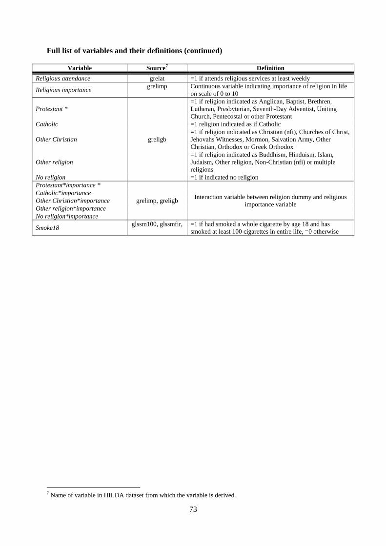
73
Full list of variables and their definitions (continued)
Variable Source7 Definition Religious attendance grelat =1 if attends religious services at least weekly
Religious importance grelimp Continuous variable indicating importance of religion in life on scale of 0 to 10
Protestant *
greligb
=1 if religion indicated as Anglican, Baptist, Brethren, Lutheran, Presbyterian, Seventh-Day Adventist, Uniting Church, Pentecostal or other Protestant
Catholic =1 religion indicated as if Catholic
Other Christian =1 if religion indicated as Christian (nfi), Churches of Christ, Jehovahs Witnesses, Mormon, Salvation Army, Other Christian, Orthodox or Greek Orthodox
Other religion =1 if religion indicated as Buddhism, Hinduism, Islam, Judaism, Other religion, Non-Christian (nfi) or multiple religions
No religion =1 if indicated no religion Protestant*importance *
grelimp, greligb Interaction variable between religion dummy and religious importance variable
Catholic*importance Other Christian*importance Other religion*importance No religion*importance
Smoke18 glssm100, glssmfir, =1 if had smoked a whole cigarette by age 18 and has smoked at least 100 cigarettes in entire life, =0 otherwise
7 Name of variable in HILDA dataset from which the variable is derived.

74
Appendix 5: Log earnings results assuming exogenous selection
Variable Abstainer Moderate Drinker Heavy Drinker Coefficient
(Standard Error) Coefficient
(Standard Error) Coefficient
(Standard Error) Constant 7.0142*** (0.1659) 7.3424*** (0.0593) 7.3095*** (0.0930) Age 25-29 -0.0273 (0.1359) -0.3522*** (0.0529) -0.0118 (0.0775) Age 30-34 -0.1133 (0.1004) -0.0942* (0.0487) 0.0110 (0.0717) Age 35-39 0.0133 (0.1220) -0.1297*** (0.0502) -0.0632 (0.0814) Age 45-49 0.0551 (0.1257) -0.0883* (0.0463) 0.0017 (0.0781) Age 50-59 -0.0734 (0.1154) -0.2162*** (0.0664) 0.0672 (0.0918) Age 60-64 0.1426 (0.1428) -0.1569*** (0.0557) 0.0831 (0.0947) Single -0.1554** (0.0702) -0.1232*** (0.0412) -0.0915** (0.0440) Immigrant English-speaking 0.0388 (0.0703) -0.0105 (0.0481) 0.0212 (0.0840) Immigrant other 0.0330 (0.0906) -0.1418*** (0.0541) -0.0936 (0.0655) VIC 0.0937 (0.0897) -0.0491 (0.0406) -0.0664 (0.0565) QLD 0.1545 (0.0983) -0.0576 (0.0414) 0.0026 (0.0611) SA 0.0290 (0.1194) -0.1100** (0.0437) -0.2005** (0.0891) WA 0.1302 (0.1126) 0.0604 (0.0543) 0.0900 (0.0833) TAS -0.0694 (0.1435) -0.1384* (0.0749) -0.0014 (0.0953) NT -0.0066 (0.1614) 0.0275 (0.2126) -0.0131 (0.1649) ACT 0.2168 (0.1554) -0.0713 (0.0693) 0.2097 (0.2044) Regional 0.0099 (0.0737) -0.0844** (0.0328) -0.0771 (0.0551) Remote -0.0777 (0.1905) -0.1369 (0.1460) -0.0407 (0.1833) Postgraduate degree 0.3053* (0.1554) 0.3227*** (0.0601) 0.2285* (0.1211) Undergraduate 0.1174 (0.0862) 0.1757*** (0.0468) 0.0104 (0.0694) Year 12 -0.0378 (0.0700) -0.0099 (0.0506) -0.0931 (0.0824) Did not complete High School -0.2706*** (0.0985) -0.1051** (0.0427) -0.1326** (0.0547) Managers 0.0495 (0.1135) 0.0645 (0.0478) -0.0546 (0.0854) Technicians & Trades -0.1733 (0.1181) -0.0875 (0.0537) -0.2934*** (0.0786) Community & Personal Services -0.0834 (0.1064) -0.1485** (0.0652) -0.1540 (0.1045) Clerical & Administrative -0.1791 (0.1098) -0.1144** (0.0509) -0.1362 (0.0849) Sales -0.1700 (0.1317) -0.3275*** (0.0831) -0.2131* (0.1233) Machinery operators -0.0806 (0.1080) -0.0413 (0.0661) -0.2789*** (0.0904) Labourers -0.4504** (0.1952) -0.1633** (0.0642) -0.2949*** (0.0936) Public sector 0.0498 (0.0574) 0.0127 (0.0320) 0.0120 (0.0549) Number of observations 438 1241 473 R-Squared 0.2628 0.2078 0.1721

75
Appendix 6: Log earnings results (religious attendance excluded)
Variable Abstainer Moderate Drinker Heavy Drinker Coefficient
(Standard Error) Coefficient
(Standard Error) Coefficient
(Standard Error) Constant 6.8418*** (0.2175) 7.4310*** (0.1340) 7.4775*** (0.1589) IMR 0.1589* (0.0955) -0.1166 (0.1645) -0.1228 (0.0999) Age 25-29 -0.0585 (0.1334) -0.3588*** (0.0533) -0.0285 (0.0784) Age 30-34 -0.1440 (0.0984) -0.1031** (0.0511) -0.0038 (0.0737) Age 35-39 0.0076 (0.1211) -0.1375*** (0.0514) -0.0482 (0.0811) Age 45-49 0.0358 (0.1230) -0.1009** (0.0496) 0.0115 (0.0784) Age 50-59 -0.1035 (0.1135) -0.2351*** (0.0707) 0.0814 (0.0928) Age 60-64 0.1204 (0.1416) -0.1674*** (0.0581) 0.1066 (0.0965) Single -0.1376** (0.0690) -0.1077** (0.0473) -0.1045** (0.0452) Immigrant English-speaking 0.0303 (0.0708) -0.0168 (0.0485) 0.0161 (0.0830) Immigrant other 0.1157 (0.1135) -0.1242* (0.0635) -0.0304 (0.0851) VIC 0.0760 (0.0887) -0.0550 (0.0420) -0.0724 (0.0569) QLD 0.1398 (0.0980) -0.0678 (0.0443) 0.0145 (0.0618) SA -0.0071 (0.1206) -0.1264** (0.0499) -0.1923** (0.0862) WA 0.1240 (0.1125) 0.0654 (0.0543) 0.0943 (0.0843) TAS -0.1004 (0.1485) -0.1573** (0.0799) 0.0166 (0.1008) NT -0.0853 (0.1932) 0.0541 (0.2221) -0.0911 (0.1755) ACT 0.2191 (0.1587) -0.0858 (0.0740) 0.2772 (0.2220) Regional -0.0036 (0.0732) -0.0791** (0.0338) -0.0995* (0.0557) Remote -0.1180 (0.1805) -0.1303 (0.1479) -0.0727 (0.1857) Postgraduate degree 0.2534* (0.1537) 0.2883*** (0.0771) 0.2497** (0.1218) Undergraduate 0.0900 (0.0848) 0.1594*** (0.0533) 0.0235 (0.0712) Year 12 -0.0326 (0.0710) -0.0101 (0.0505) -0.0923 (0.0824) Did not complete High School -0.2758*** (0.0983) -0.0858* (0.0506) -0.1564*** (0.0546) Managers 0.0332 (0.1131) 0.0567 (0.0474) -0.0488 (0.0853) Technicians & Trades -0.1836 (0.1166) -0.0841 (0.0546) -0.3045*** (0.0789) Community & Personal Services -0.0465 (0.1102) -0.1297* (0.0722) -0.1506 (0.1038) Clerical & Administrative -0.1689 (0.1108) -0.1072** (0.0527) -0.1285 (0.0844) Sales -0.1388 (0.1374) -0.3248*** (0.0835) -0.1844 (0.1270) Machinery operators -0.0607 (0.1092) -0.0233 (0.0724) -0.2914*** (0.0900) Labourers -0.4229** (0.1908) -0.1462** (0.0701) -0.3102*** (0.0940) Public sector 0.0448 (0.0571) 0.0105 (0.0320) 0.0168 (0.0545) Number of observations 438 1241 473 R-squared 0.2673 0.2083 0.1751

76
Appendix 7: Heckman selection results using NHMRC definition
Variable Abstainers Heavy Drinkers Marginal effects on probabilities Coefficient
(Standard Error) Coefficient
(Standard Error) Abstainer Moderate Drinker
Heavy Drinker
Predicted Probability Constant -0.4523 (0.4002) 0.2775 (0.3034) 0.1860 0.2638 0.5503 Marginal Effect Age 25-29 -0.6081* (0.3560) 0.3636 (0.2476) -0.1065 -0.0326 0.1391 Age 30-34 -0.3979 (0.3060) 0.1962 (0.2204) -0.0719 -0.0128 0.0846 Age 35-39 -0.2229 (0.2855) -0.0693 (0.2079) -0.0257 0.0210 0.0046 Age 45-49 -0.3942 (0.2953) -0.3719* (0.2136) -0.0225 0.0776 -0.0551 Age 50-59 -0.7306** (0.2872) -0.5220** (0.2205) -0.0551 0.1210 -0.0659 Age 60-64 -0.2157 (0.3747) -0.2026 (0.2529) -0.0122 0.0415 -0.0293 Single 0.5031** (0.2253) 0.3718** (0.1631) 0.0384 -0.0749 0.0365 Immigrant English-speaking -0.2401 (0.2740) 0.0087 (0.1994) -0.0350 0.0097 0.0252 Immigrant other 0.3869 (0.2813) -0.5058** (0.2418) 0.1241 0.0440 -0.1681 VIC -0.3107 (0.2292) 0.0099 (0.1656) -0.0458 0.0130 0.0327 QLD -0.3998 (0.2661) -0.0708 (0.1868) -0.0498 0.0293 0.0205 SA -0.6548* (0.3385) -0.0703 (0.2416) -0.0776 0.0388 0.0388 WA 0.2117 (0.2986) 0.0668 (0.2229) 0.0262 -0.0200 -0.0062 TAS -1.0362** (0.4763) -0.5678* (0.3264) -0.0839 0.1468 -0.0629 NT -1.0035 (0.9146) 0.0952 (0.6422) -0.1140 0.0180 0.0960 ACT -0.0384 (0.5168) -0.3002 (0.3749) 0.0245 0.0464 -0.0709 Regional -0.0246 (0.2021) 0.3140** (0.1473) -0.0353 -0.0441 0.0794 Remote 0.5282 (0.6903) 1.1194** (0.4948) -0.0464 -0.1488 0.1951 Postgraduate degree -1.1745*** (0.4033) -0.3931 (0.2638) -0.1066 0.1169 -0.0103 Undergraduate -0.4292* (0.2523) -0.3884** (0.1774) -0.0258 0.0812 -0.0554 Year 12 0.0878 (0.3087) -0.0558 (0.2098) 0.0195 0.0035 -0.0230 Did not complete High School 0.4479* (0.2715) 0.5871*** (0.2062) 0.0042 -0.0978 0.0936 Managers -0.1859 (0.2964) -0.1185 (0.1890) -0.0158 0.0268 -0.0110 Technicians & Trades 0.3128 (0.2793) 0.5341*** (0.2054) -0.0097 -0.0872 0.0968 Community & Personal Services 1.5487*** (0.4444) 0.8648*** (0.3277) 0.1690 -0.1616 -0.0074 Clerical & Administrative 0.6148* (0.3712) 0.4466* (0.2440) 0.0482 -0.0862 0.0380 Sales 0.0878 (0.3938) -0.3780 (0.3331) 0.0544 0.0490 -0.1034 Machinery operators 0.7395** (0.3525) 0.4399 (0.2712) 0.0712 -0.0914 0.0201 Labourers 0.6073 (0.3747) 0.2357 (0.3143) 0.0750 -0.0616 -0.0134 Public sector -0.0474 (0.2313) 0.0410 (0.1705) -0.0112 -0.0037 0.0149 Religious attendance 0.6184** (0.3003) -0.3926 (0.3018) 0.1606 0.0092 -0.1698 Religious importance 0.0710 (0.0451) -0.0840** (0.0349) 0.0193 0.0087 -0.0281 Catholic 0.2912 (0.4081) 0.0582 (0.2633) 0.0396 -0.0229 -0.0167 Other Christian 0.6538 (0.8199) -0.1336 (0.5835) 0.1363 -0.0236 -0.1127 Other religion -0.7844 (0.9038) -0.9804 (0.6293) -0.0314 0.2083 -0.1769 No religion 0.1397 (0.2938) 0.0649 (0.1866) 0.0146 -0.0162 0.0016 Catholic*importance -0.0698 (0.0693) 0.0626 (0.0555) -0.0170 -0.0057 0.0226 Other Christian*importance -0.0497 (0.1139) 0.0900 (0.0921) -0.0167 -0.0106 0.0274 Other religion*importance 0.2372* (0.1290) 0.2998*** (0.1007) 0.0052 -0.0551 0.0499 No religion*importance 0.1778 (0.1151) 0.1525 (0.0950) 0.0113 -0.0309 0.0196 Smoke18 -0.2696 (0.1965) 0.5837*** (0.1275) -0.0991 -0.0708 0.1699 Number of observations 2152 Log-likelihood -1934.1088

77
Variable Abstainer Moderate Drinker Heavy Drinker Coefficient
(Standard Error) Coefficient
(Standard Error) Coefficient
(Standard Error) Constant 6.9539*** (0.2189) 7.4787*** (0.2075) 7.4125*** (0.0831) IMR 0.0473 (0.0861) -0.1878 (0.1594) -0.0765 (0.0801) Age 25-29 -0.1420 (0.1735) -0.3239*** (0.0808) -0.1604*** (0.0503) Age 30-34 -0.1470 (0.1232) -0.1163 (0.0713) -0.0307 (0.0487) Age 35-39 0.0282 (0.1474) -0.1944** (0.0799) -0.0458 (0.0501) Age 45-49 0.0743 (0.1385) -0.1801** (0.0701) 0.0070 (0.0489) Age 50-59 -0.1169 (0.1361) -0.3103*** (0.1068) -0.0133 (0.0575) Age 60-64 0.1759 (0.1731) -0.1479* (0.0872) -0.0532 (0.0518) Single -0.1730** (0.0844) -0.0274 (0.0739) -0.1706*** (0.0324) Immigrant English-speaking 0.0483 (0.0819) 0.0297 (0.0772) 0.0008 (0.0460) Immigrant other 0.0071 (0.1171) -0.1024 (0.0776) -0.0579 (0.0550) VIC 0.1429 (0.1083) -0.0571 (0.0618) -0.0589 (0.0367) QLD 0.2088* (0.1178) 0.0246 (0.0628) -0.0809** (0.0373) SA 0.0705 (0.1476) -0.0740 (0.0645) -0.1735*** (0.0484) WA 0.1466 (0.1312) 0.0174 (0.0824) 0.0959* (0.0541) TAS -0.0794 (0.1737) -0.1821** (0.0874) -0.0742 (0.0800) NT 0.0435 (0.1979) 0.0038 (0.2428) -0.0279 (0.1444) ACT 0.2955* (0.1677) -0.0384 (0.1015) -0.0335 (0.0893) Regional 0.0118 (0.0935) -0.1161** (0.0525) -0.0567* (0.0332) Remote -0.0753 (0.2083) -0.5325 (0.3334) -0.0477 (0.1155) Postgraduate degree 0.3393** (0.1716) 0.3131*** (0.0858) 0.2577*** (0.0802) Undergraduate 0.1493* (0.0879) 0.1683** (0.0759) 0.0923** (0.0450) Year 12 -0.0171 (0.0833) 0.0326 (0.0783) -0.0516 (0.0455) Did not complete High School -0.3825*** (0.1192) -0.0455 (0.0923) -0.1570*** (0.0352) Managers 0.0451 (0.1241) 0.1580** (0.0665) -0.0530 (0.0479) Technicians & Trades -0.1805 (0.1272) -0.0497 (0.0809) -0.2167*** (0.0510) Community & Personal Services -0.0259 (0.1267) -0.1574 (0.1007) -0.1497** (0.0663) Clerical & Administrative -0.1954* (0.1103) -0.0360 (0.0707) -0.1701*** (0.0550) Sales -0.2278 (0.1472) -0.4290*** (0.1024) -0.1568** (0.0791) Machinery operators -0.0953 (0.1187) -0.0225 (0.1070) -0.1547*** (0.0597) Labourers -0.4248* (0.2274) -0.1784* (0.0914) -0.2670*** (0.0638) Public sector -0.0022 (0.0647) 0.0826* (0.0489) -0.0042 (0.0343) Number of observations 351 606 1195 R-squared 0.3076 0.2419 0.1911

78
Appendix 8: Heckman selection results using alternative definition
Variable Abstainers Heavy Drinkers Marginal effects on probabilities Coefficient
(Standard Error) Coefficient
(Standard Error) Abstainer Moderate Drinker
Heavy Drinker
Predicted Probability Constant -1.0027*** (0.3181) -2.8795*** (0.5372) 0.2341 0.7025 0.0634 Marginal Effect Age 25-29 -0.4110 (0.2677) 0.5679* (0.3129) -0.0762 0.0276 0.0486 Age 30-34 -0.4987** (0.2451) 0.3334 (0.3004) -0.0858 0.0558 0.0300 Age 35-39 -0.0938 (0.2354) -0.1737 (0.3101) -0.0142 0.0227 -0.0086 Age 45-49 -0.3713 (0.2500) -0.4987 (0.3143) -0.0565 0.0782 -0.0218 Age 50-59 -0.5590** (0.2310) -0.4851 (0.3864) -0.0845 0.1037 -0.0193 Age 60-64 -0.1818 (0.3070) -0.3651 (0.3676) -0.0269 0.0440 -0.0171 Single 0.4485** (0.1822) 0.6462*** (0.1942) 0.0725 -0.1075 0.0350 Immigrant English-speaking -0.3032 (0.2245) -0.4020 (0.3467) -0.0463 0.0639 -0.0176 Immigrant other 0.7985*** (0.2385) -0.3086 (0.3999) 0.1686 -0.1409 -0.0277 VIC -0.2323 (0.1935) 0.1438 (0.2476) -0.0425 0.0301 0.0124 QLD -0.2075 (0.2183) 0.0540 (0.2478) -0.0367 0.0304 0.0063 SA -0.4722* (0.2691) -0.0591 (0.3479) -0.0749 0.0723 0.0026 WA 0.2673 (0.2494) 0.4447 (0.3261) 0.0420 -0.0671 0.0252 TAS -0.3442 (0.4228) 0.3074 (0.4670) -0.0606 0.0338 0.0267 NT -0.9574 (0.7671) 1.5130** (0.6040) -0.1517 -0.0494 0.2011 ACT 0.1428 (0.4401) -0.7194 (0.8232) 0.0351 -0.0020 -0.0330 Regional -0.2203 (0.1681) 0.3686* (0.1932) -0.0440 0.0168 0.0272 Remote -0.5011 (0.5335) 0.0982 (0.5585) -0.0794 0.0663 0.0131 Postgraduate degree -1.1957*** (0.3771) -0.2279 (0.5592) -0.1546 0.1561 -0.0015 Undergraduate -0.4817** (0.2179) 0.0102 (0.3076) -0.0804 0.0731 0.0073 Year 12 0.0716 (0.2416) 0.2332 (0.2848) 0.0092 -0.0229 0.0137 Did not complete High School 0.1926 (0.2089) 0.5203** (0.2336) 0.0261 -0.0581 0.0320 Managers -0.1509 (0.2625) 0.0046 (0.3244) -0.0264 0.0239 0.0025 Technicians & Trades 0.0339 (0.2387) 0.2277 (0.3432) 0.0025 -0.0162 0.0137 Community & Personal Services 0.8728** (0.3638) 0.6510 (0.4765) 0.1681 -0.1927 0.0247 Clerical & Administrative 0.3512 (0.2967) -0.0315 (0.4175) 0.0681 -0.0608 -0.0073 Sales 0.3197 (0.3373) -0.6650 (0.8256) 0.0704 -0.0370 -0.0334 Machinery operators 0.6323** (0.2710) 0.8383** (0.3932) 0.1064 -0.1545 0.0481 Labourers 0.4129 (0.2965) 0.6753 (0.4249) 0.0654 -0.1062 0.0408 Public sector -0.0195 (0.1949) 0.0735 (0.2444) -0.0046 -0.0002 0.0047 Religious attendance 0.7022*** (0.2670) -0.7907 (0.7541) 0.1550 -0.1125 -0.0425 Religious importance 0.0927** (0.0390) -0.0679 (0.0590) 0.0176 -0.0122 -0.0054 Catholic 0.1025 (0.3337) -0.1984 (0.3301) 0.0215 -0.0088 -0.0127 Other Christian 0.5672 (0.6839) -0.9501 (0.9948) 0.1272 -0.0837 -0.0435 Other religion -0.4045 (0.7174) -0.6515 (0.8703) -0.0594 0.0865 -0.0271 No religion -0.0345 (0.2402) 0.0516 (0.2542) -0.0069 0.0033 0.0036 Catholic*importance -0.0509 (0.0599) 0.1245 (0.0808) -0.0110 0.0028 0.0081 Other Christian*importance -0.0682 (0.0948) 0.2102 (0.1592) -0.0153 0.0019 0.0135 Other religion*importance 0.0775 (0.1029) -0.2426 (0.2525) 0.0175 -0.0019 -0.0155 No religion*importance 0.0863 (0.0818) -0.1528 (0.1332) 0.0177 -0.0074 -0.0104 Smoke18 -0.3787** (0.1594) 0.5743*** (0.1908) -0.0760 0.0353 0.0407 Number of observations 2152 Log-likelihood -1615.609

79
Variable Abstainer Moderate Drinker Heavy Drinker Coefficient
(Standard Error) Coefficient
(Standard Error) Coefficient
(Standard Error) Constant 6.8226*** (0.2197) 7.4060*** (0.0936) 7.3073*** (0.3201) IMR 0.1829* (0.0996) -0.1140 (0.1538) -0.1003 (0.1367) Age 25-29 -0.0658 (0.1299) -0.3055*** (0.0482) 0.0134 (0.1105) Age 30-34 -0.1524 (0.0960) -0.0593 (0.0444) -0.0282 (0.1024) Age 35-39 0.0050 (0.1198) -0.1313*** (0.0460) 0.0771 (0.0982) Age 45-49 0.0318 (0.1211) -0.0933** (0.0438) 0.1773 (0.1109) Age 50-59 -0.1048 (0.1100) -0.1847*** (0.0642) 0.1551 (0.1143) Age 60-64 0.1163 (0.1395) -0.1136** (0.0498) 0.0375 (0.1681) Single -0.1362** (0.0683) -0.0855** (0.0395) -0.1320** (0.0667) Immigrant English-speaking 0.0282 (0.0707) -0.0171 (0.0448) 0.0955 (0.1445) Immigrant other 0.1288 (0.1181) -0.1114 (0.0699) -0.0451 (0.1007) VIC 0.0743 (0.0886) -0.0558 (0.0371) -0.0158 (0.0868) QLD 0.1379 (0.0976) -0.0584 (0.0378) 0.0401 (0.0821) SA -0.0129 (0.1190) -0.1649*** (0.0462) 0.0211 (0.1155) WA 0.1249 (0.1117) 0.0935* (0.0557) 0.0883 (0.0808) TAS -0.0978 (0.1496) -0.1548** (0.0674) 0.1269 (0.1158) NT -0.1104 (0.1957) -0.0225 (0.1947) 0.0686 (0.2008) ACT 0.2147 (0.1566) -0.0425 (0.0695) 0.0045 (0.2430) Regional -0.0066 (0.0719) -0.0710** (0.0299) -0.1121 (0.0798) Remote -0.1393 (0.1804) -0.1728 (0.1284) 0.2988 (0.1887) Postgraduate degree 0.2401 (0.1602) 0.2617*** (0.0668) 0.4453** (0.1768) Undergraduate 0.0845 (0.0835) 0.1373*** (0.0461) 0.0449 (0.0894) Year 12 -0.0320 (0.0705) -0.0306 (0.0465) -0.0338 (0.0967) Did not complete High School -0.2752*** (0.0977) -0.1316*** (0.0399) -0.0484 (0.0778) Managers 0.0267 (0.1131) 0.0459 (0.0436) -0.0549 (0.1274) Technicians & Trades -0.1888 (0.1165) -0.1398*** (0.0483) -0.1924* (0.1132) Community & Personal Services -0.0495 (0.1082) -0.1297* (0.0753) -0.1548 (0.1463) Clerical & Administrative -0.1748 (0.1097) -0.0984** (0.0474) -0.1987 (0.1266) Sales -0.1365 (0.1361) -0.3025*** (0.0731) -0.0124 (0.1928) Machinery operators -0.0638 (0.1080) -0.0319 (0.0697) -0.3711*** (0.1261) Labourers -0.4233** (0.1869) -0.1630** (0.0669) -0.3556*** (0.1138) Public sector 0.0471 (0.0570) 0.0019 (0.0305) 0.1227 (0.0748) Number of observations 439 1489 224 R-squared 0.2700 0.1930 0.2629

80
10. REFERENCES ABS (2006), National Health Survey: Users’ Guide – Electronic Publication,
Commonwealth of Australia. Ashley, M.J., Rehm, J., Bondy, S., Single, E. & Rankin, J. (2000), “Beyond ischemic heart
disease: are there other health benefits from drinking alcohol?”, Contemporary Drug Problems, vol 27: 735-777.
Auld, C. (2005), "Smoking, Drinking and Income", Journal of Human Resources, vol. 40:
505-518. Barrett, G. (2002), "The effect of Alcohol Consumption on Earnings", The Economic Record,
vol. 78, no. 1, pp. 79-96. Baglietto, L., English, D.R., Hopper, J.L., Powles, J. & Giles, G.G. (2006), “Average volume
of alcohol consumed, type of beverage, drinking pattern and the risk of death from all causes”, Alcohol and Alcoholism, vol. 41, no. 56: 664–71.
Berger, M.C. & Leigh, J.P. (1988), "The effect of alcohol use on wages", Applied Economics,
vol. 20, pp.1343-1351. Bryson, C.L, Mukamal, K.J., Mittleman, M.A, Fried, L.P., Hirsch, C.H., Kitzman, D.W. &
Siscovick, D.S. (2006), “The association of alcohol consumption and incident heart failure”, Journal of the American College of Cardiology, vol. 48: 305–11.
Di Castelnuovo, A., Rotondo, S., Iacoviello, L., Donati, M.D. & de Gaetano, G. (2002),
“Meta-analysis of wine and beer consumption in relation to vascular risk”, Circulation, vol. 105, no. 24: 2836–44.
"Feng, W. Et al (2001), "The impact of problem drinking on employment", Health
Economics, vol. 10: 509-521. Hamilton, V. & Hamilton, B.H. (1997), "Alcohol and earnings: does drinking yield a wage
premium?", Canadian Journal of Economics, vol. 30, no. 1, pp.135-151. Heckman, J.J. (1979), “Sample selection bias as a specification error”, Econometrica, vol. 47,
no. 1: 153-161. Heineck, G. & Schwarze, J. (2003), "Substance use and earnings: The case of smokers in
Germany", IZA Discussion Paper, no. 743. Idson, T.L. & Feaster, D.J. (1990), “A selectivity model of employer-size differentials”,
Journal of Labor Economics, vol. 8, no. 1: 99-122. Johansson, E., Alho, H., Kiiskinen, U. & Poikolainen, K. (2007), "The association of alcohol
dependency with employment probability: evidence from the population survey 'Health 2000 in Finland'", Health Economics, vol. 16: 739-754.

81
Keng, S.H. & Huffman, W.E. (2005), "Binge drinking and labor market success: a longitudinal study on young people", Journal of Population Economics, vol. 20: 35-54.
Kenkel, D.S., Ribar, D.C., Cook, P.J., Peltzman, S. (1994), "Alcohol consumption and young
adults' socioeconomic status", Brookings Papers on Economic Activity: Microeconomics, vol. 1994: 119-175.
Kenkel, D. & Wang, P. (1998), "Are alcoholics in bad jobs?", NBER Working Paper Series,
Working Paper 6401. Lee, L.-F. (1982), "Some Approaches to the Correction of Selectivity Bias", Review of
Economic Studies, vol. 49: 355-372. Levine, P.B., Gustafson, T.A. & Velenchik, A.D. (1997), "More bad news for smokers? The
effects of cigarette smoking on wages", Industrial & Labor Relations Review, vol. 50, no. 3: 493-509.
Little, R.J.A., & Su, H.L. (1989), “Item Non-Response in Panel Surveys” in Panel Surveys,
edited by Kasprzyk, D., Duncan, G.J., Kalton, G., Singh, M.P., John Wiley and Sons, New York.
Lye, J.N. & Hirschberg, J. (2004), "Alcohol consumption, smoking and wages", Applied
Economics, vol. 36, pp.1807-1817. MacDonald, Z. & Shields, M.A. (2004), "Does problem drinking affect employment?
Evidence from England", Health Economics, vol. 13: 139-155. Mullahy, J. & Sindelar, J.L. (1993), "Alcoholism, Work and Income", Journal of Labor
Economics, vol. 11, no. 3: 494-520. Mullahy, J. & Sindelar, J. (1996), "Employment, unemployment and problem drinking",
Journal of Health Economics, vol. 15: 409-434. NHMRC (2001) Australian Alcohol Guidelines: Health risks and benefits, Commonwealth of
Australia. NHMRC (2009a) “About”, http://www.nhmrc.gov.au/about/index.htm. NHMRC (2009b) Australian Guidelines: To reduce health risks from drinking alcohol,
Commonwealth of Australia. NIH (2009a) Rethinking Drinking: Alcohol and your health, National Institute of Health. NIH (2009a) “NIH Mission”, http://www.nih.gov.au/about/#mission. Oaxaca, R. (1973), “Male-female wage differentials in urban labor markets”, International
Economic Review, vol. 14: 693-709. Renna, F. (2008), "Alcohol abuse, alcoholism and labour market outcomes: looking for the
missing link", Industrial and Labor Relations Review, vol. 62, no. 1: 92-103.

82
Sinclair, L. (2008a), ‘Labor set to fall off the ad wagon’, The Australan, 31 March, p. 34. Sinclair, L. (2008b), ‘Sport to suffer if alcohol ads stop’, The Australian, 27 March, p. 36. Terza, J.V. (2002), "Alcohol abuse and employment: A second look", Journal of Applied
Econometrics, vol. 17: 393-404. van Ours, J.C. (2004), "A pint a day raises a man's pay; but smoking blows that gain away",
Journal of Health Economics, vol. 23, pp.863-886. Verster, J.C., Duin D.V., Volkerts, E.R., Schreuder, A. & Verbaten, M.N. (2003), “Alcohol
hangover effects on memory functioning and vigilance performance after an evening of binge drinking”, Neuropsychopharmacology, vol. 28: 740–46.
Watson, N. (ed.) (2009), HILDA User Manual – Release 7, Melbourne Institute of Applied
Economic and Social Research, University of Melbourne.