the effects of interregional trade flow estimating … · 2017-09-11 · the effects of...

The Effects of Interregional Trade Flow Estimating Proce-dures on Multiregional Social Accounting Matrix Multipliers Dennis P. Robinson and Zuoming Liu University of Missouri, Columbia - USA

Abstract. Social accounting matrix (SAM) models have become standard methods to provide quantitative economic impact evaluation. SAM models and methods have a wide body of lit-erature and dates back several decades. In recent years there has been a growing interest in us-ing interregional and multiregional SAM models. IMPLAN provides data necessary, in a con-venient format, to construct single-region SAM models. Procedures of the use of IMPLAN data in concert with BEA’s “journey-to-work” commuting flows and data from the Commodity Flow Survey (CFS) collected by the Census Bureau and compiled by the Bureau of Transporta-tion Statistics to construct state-level multiregional SAM models has been demonstrated. How-ever, little research exists concerning the creation of multiregional SAM models at geographic scales lower than states, especially the roll that interregional trade plays in the accuracy of these models. This paper evaluates sensitivity of multiregional SAM multipliers to the procedures used to estimate interregional trade flows.

1. Introduction Social accounting matrix (SAM) models are impor-tant quantitative economic evaluation tools. These models permit an assessment of different policy deci-sions over an entire economic system using the effects of important economic aggregates and agents. There is a wide body of literature on SAM models and meth-ods that date back several decades. In recent years there has been a growing interest in using interre-gional and multiregional SAM models. IMPLAN provides data in a convenient format that are necessary to construct single region input-output and SAM models. In order to compile a work-ing multiregional input-output or SAM model, how-ever, a set of interregional trade flows (or coefficients) have to be estimated. The use of IMPLAN data in concert with data from the Commodity Flow Survey (CFS)—collected by the Census Bureau and compiled by the Bureau of Transportation Statistics—to con-struct state-level multiregional SAM model has been demonstrated by Jackson (2002). However, little re-search exists concerning the creation of multiregional models at geographic scales lower than states, espe-cially the roll that interregional trade plays.

This paper evaluates the effects of using two inter-regional trade flow estimating procedures on multire-gional SAM multipliers. One uses a variation of loca-tion quotient to estimate domestic exports. The other uses the regional purchase coefficients that IMPLAN produces to estimate domestic imports. The estimated domestic imports and exports for both sets of trade flow estimates are balanced to fit within IMPLAN’s accounting framework. The techniques employed in this paper are applied to 238, 3-region multiregional SAM models. Section 2 provides the motivation for compiling multiregional SAM models and their use in measuring the performance of a major federal government agency. The information system and multiregional SAM models that were developed for the agency are described. Section 3 of the paper explains the two techniques that were used to estimate the interregional commodity trade flows—based on location quotients and on regional purchase coefficients. Comparisons of the variability in the multipliers and impact estimates that result by using different trade flow estimating procedures are shown in section 4. Finally, section 5 provides several conclusions and recommendations.

MCRSA Presidential Symposium – 36th Annual Conference; JRAP 36(1): 94-114. © 2006 MCRSA. All rights reserved.

Trade flow and SAM multipliers 95

2. Measuring Development Performance The mission of the United States Department of Agriculture Rural Development program (formerly known as the Rural Business-Cooperative Services or RBS) is to promote a dynamic business environment in rural America. Rural Development uses a variety of loan and grant programs to help facilitate projects that create or preserve quality jobs and enhance the quality of life in rural communities across the nation. Rural Development works in partnership with the private sector and community-based organizations to provide financial assistance to meet business and credit need in under-served areas. Recently, the USDA Economic Research Service has entered into a cooperative agreement with the Community Policy Analysis Center (CPAC) and the Rural Policy Research Institute (RUPRI) to develop an information system and set of multiregional SAM models to assess the effectiveness of the Rural Devel-opment loan and grant programs (Robinson and John-son, 2005). The resulting information system is called the Rural Development Socio-Economic Benefits As-sessment System (SEBAS). SEBAS has to date been developed for California, Montana, New Hampshire, North Carolina, and Vermont. 2.1 Expanding criteria for measuring Performance Currently, Rural Development reports jobs either created or retained by its loan and grant recipients. “Direct” jobs increases are used by many federal and state agencies as a measure of their performance. However, the number of direct jobs created or retained is, in isolation, a poor indicator of economic change and performance. For example, reporting direct jobs treats part-time and full-time jobs equally despite the fact that full-time jobs generate more income, more security and support families better. Job estimates should be adjusted to reflect full-time equivalency (FTE). This provides a performance measure that doesn’t ignore seasonal and part-time work but would give greater weight to projects that produce full-time jobs compared to part-time jobs. But even full-time employment is too narrow a measure of economic performance. With SEBAS, Ru-ral Development is able to track and report contribu-tions to gross domestic product (GDP) from its pro-jects.1 GDP is the broadest available measure of in-come and the most widely used measure of macro-

1 GDP is defined here as value added—the sum of employee com-pensation, proprietors’ income, other property type income, and indirect business taxes.

economic performance. It is the sum of four impact variables estimated by SEBAS: employee compensa-tion (wages and salaries plus employee benefits), pro-prietors’ income, other property-type income (profits, dividends, interest, rents, etc.), and indirect business taxes. Direct changes in jobs, employment and contribu-tions to GDP are perhaps the best measures of change at a national accounting level. But at the local and re-gional level, linkages between sectors are critical de-terminants of change in the economic well-being. To-tal economic effects (direct and indirect) reflect the impact of programs on the activities of existing firms in a local economy. Finally, the “quality” of the jobs created by Rural Development loans and grants should be a key indica-tor of its performance. Those employers that pay higher wages, more benefits, and contribute to the tax base, and those that indirectly stimulate existing firms that pay higher wages, more benefits and contribute to the tax base, will contribute more to the local, rural community welfare. This factor can be measured by the ratio of GDP to FTE or the “GDP per worker” ra-tio. 2.2 What SEBAS Does and Does Not Do? SEBAS offers an opportunity to consider a much wider and richer array of assessment criteria. The ar-ray is “wider” because SEBAS tracks a greater number of possible assessment criteria than just the number of jobs created or retained. The array is “richer” for two important reasons. First, SEBAS not only considers the direct effects of RBS’ activity, but it also addresses the indirect effects of the loan and grant programs. Second, SEBAS provides an evaluation of the geo-graphic dispersion of Rural Development’s social and economic effects by measuring the impacts at the county, region and state levels. But SEBAS is more than these key indicators. In addition to the indicators listed above, SEBAS also generates a variety of economic impact measures that may be useful when more detailed and inclusive ac-counts of particular projects are desired. These meas-ures include such evaluation information as business sales, personal income, indirect business taxes, an im-plicit wage for the overall impact, and federal, state, and local taxes. SEBAS also generates estimates of how Rural Development loans and grants affect the distribution of household income, the occupational distribution of employment impacts, and the genera-tion of various types of tax revenues. SEBAS focuses on the mission of the Rural Devel-opment, which is to improve the quality of life in rural

96 Robinson and Liu

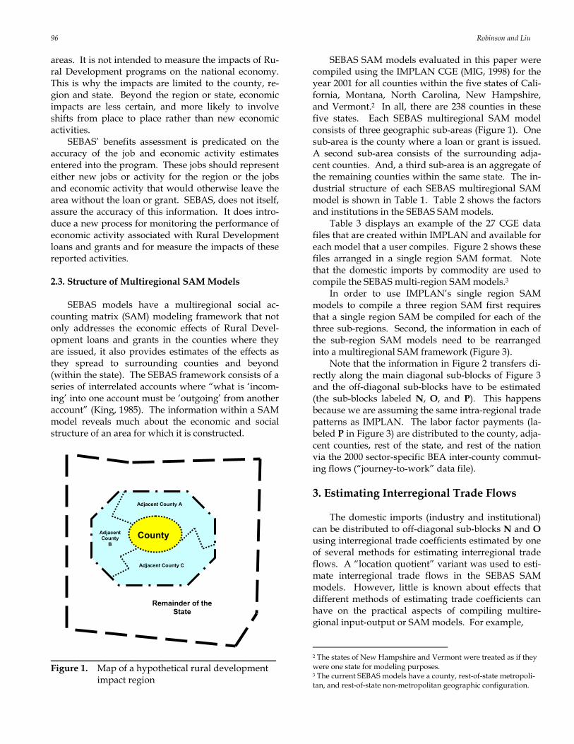
areas. It is not intended to measure the impacts of Ru-ral Development programs on the national economy. This is why the impacts are limited to the county, re-gion and state. Beyond the region or state, economic impacts are less certain, and more likely to involve shifts from place to place rather than new economic activities. SEBAS’ benefits assessment is predicated on the accuracy of the job and economic activity estimates entered into the program. These jobs should represent either new jobs or activity for the region or the jobs and economic activity that would otherwise leave the area without the loan or grant. SEBAS, does not itself, assure the accuracy of this information. It does intro-duce a new process for monitoring the performance of economic activity associated with Rural Development loans and grants and for measure the impacts of these reported activities. 2.3. Structure of Multiregional SAM Models SEBAS models have a multiregional social ac-counting matrix (SAM) modeling framework that not only addresses the economic effects of Rural Devel-opment loans and grants in the counties where they are issued, it also provides estimates of the effects as they spread to surrounding counties and beyond (within the state). The SEBAS framework consists of a series of interrelated accounts where “what is ‘incom-ing’ into one account must be ‘outgoing’ from another account” (King, 1985). The information within a SAM model reveals much about the economic and social structure of an area for which it is constructed.

County

Adjacent County C

Adjacent County A

Adjacent County

B

Remainder of the State

________________________________________________ Figure 1. Map of a hypothetical rural development

impact region

SEBAS SAM models evaluated in this paper were compiled using the IMPLAN CGE (MIG, 1998) for the year 2001 for all counties within the five states of Cali-fornia, Montana, North Carolina, New Hampshire, and Vermont.2 In all, there are 238 counties in these five states. Each SEBAS multiregional SAM model consists of three geographic sub-areas (Figure 1). One sub-area is the county where a loan or grant is issued. A second sub-area consists of the surrounding adja-cent counties. And, a third sub-area is an aggregate of the remaining counties within the same state. The in-dustrial structure of each SEBAS multiregional SAM model is shown in Table 1. Table 2 shows the factors and institutions in the SEBAS SAM models. Table 3 displays an example of the 27 CGE data files that are created within IMPLAN and available for each model that a user compiles. Figure 2 shows these files arranged in a single region SAM format. Note that the domestic imports by commodity are used to compile the SEBAS multi-region SAM models.3 In order to use IMPLAN’s single region SAM models to compile a three region SAM first requires that a single region SAM be compiled for each of the three sub-regions. Second, the information in each of the sub-region SAM models need to be rearranged into a multiregional SAM framework (Figure 3). Note that the information in Figure 2 transfers di-rectly along the main diagonal sub-blocks of Figure 3 and the off-diagonal sub-blocks have to be estimated (the sub-blocks labeled N, O, and P). This happens because we are assuming the same intra-regional trade patterns as IMPLAN. The labor factor payments (la-beled P in Figure 3) are distributed to the county, adja-cent counties, rest of the state, and rest of the nation via the 2000 sector-specific BEA inter-county commut-ing flows (“journey-to-work” data file). 3. Estimating Interregional Trade Flows The domestic imports (industry and institutional) can be distributed to off-diagonal sub-blocks N and O using interregional trade coefficients estimated by one of several methods for estimating interregional trade flows. A “location quotient” variant was used to esti-mate interregional trade flows in the SEBAS SAM models. However, little is known about effects that different methods of estimating trade coefficients can have on the practical aspects of compiling multire-gional input-output or SAM models. For example,

2 The states of New Hampshire and Vermont were treated as if they were one state for modeling purposes. 3 The current SEBAS models have a county, rest-of-state metropoli-tan, and rest-of-state non-metropolitan geographic configuration.


Table 1. SEBAS multiregional SAM model commodities and sectors

Figure 2. Figure 2: Single region IMPLAN social accounting matrix format

# Commodity or Sector IMPLAN # Commodity or Sector IMPLAN1 Crops 001-010 28 Insurance 427 4282 Livestock 011-013 29 Real estate 4313 Forestry and logging 014 015 30 Utilities 030-032 495 4984 Fishing, hunting and trapping 016 017 31 Agriculture and forestry services 0185 Petroleum and natural gas 019 32 Mining services 027-0296 Mined ores 020-026 33 Printing and publishing services 136-141 413-4177 Construction 033-045 34 Internet and data process services 423 4248 Food, beverages and tobacco products 046-091 35 Motion picture and sound recording 418 4199 Textile products 092-103 36 Broadcasting 420-423

10 Apparel 104-108 37 Rental and leasing services 432-43611 Leather and allied products 109-111 38 Scientific and technical consulting services 437-45012 Wood products 112-123 39 Administrative and management support services 451-45913 Paper products 124-135 40 Waste management and remediation services 46014 Refined petroleum and coal products 142-146 41 Educational services 461-46315 Chemical products 147-171 42 Health care services 464-46816 Plastics and rubber products 172-181 43 Recreation services 471-47817 Mineral products 182-202 44 Hotels and other accomodations 479 48018 Metal products 203-256 45 Dining and drinking places 48119 Nonelectrical machinery and equipment 257-301 46 Repair and maintenance services 482-48620 Computers and electronic components 302-324 47 Personal and laundry services 487-49021 Electircal appliances and equipment 325-343 48 Religious, grantmaking and similar organizations 491-49322 Transportation equipment 344-361 49 Private households 49423 Furniture and related products 362-373 50 Social assistance services 469 47024 Other manufactured goods 374-389 51 Post office 49625 Wholesale and retail trade 390 401-412 52 Labor compensation26 Transportation 391-400 497 53 Profits, dividends, rents, interest, etc27 Finance 425 426 429 430 54 Business taxes

Industry Commodity Factor Institution Foreign TradeDomestic

Trade1 2 3 4 5 6

1 Industry Local industry make

Industry foreign exports

Industy domestic exports by commodity

Σ

2 Commodity Industry use of local commodities

Institutional use of local

commoditiesΣ

3 Factor Factor incomes Σ

4 InstitutionLocal

institutional sales

Factor distributions

Institutional transfers

Institutional foreign exports

Institutional domestic exports Σ

5 Foreign Trade Industry foreign imports

Foreign factor imports

Institutional foreign imports

Foreign transhipments Σ

6 Domestic TradeIndustry domestic

imports by commodity

Domestic factor imports

Institutional domestic imports

by commodityΣ

Total Receipts Σ Σ Σ Σ Σ Σ

Payments & Receipts

Sales and Distributions*Total Sales

and Distributions

98 Robinson and Liu

how will the estimated multiregional multipliers be impacted? In order to test the sensitivity of the mul-tiregional multiplier effects to various methods of es-timating trade flows (and, therefore, to trade coeffi-cients) an alternative method was used and compared to the location quotient procedure. Table 2. IMPLAN SAM institutions

Until recently, there were no readily available sources of interregional trade flow accounts. Com-modity trade flow surveys were conducted for 1997 and 2002 by the U.S. Bureau of the Census and the re-sults were compiled by the U.S. Bureau of Transporta-tion Statistics. However, state-to-state transport flows by commodity have not been compiled and made available for public release and use. Southworth and Pererson (2000) and Jackson, et al (2004) describe methods of estimating trade flows using data from the commodity flow survey. However, these data only cover commodity flows, not other equally important types of transactions (such as construction, trade, and services). In lieu of these vital data, Hewings, Okuyama, and Sonis (2001) and Peterson and Beck (2001) have devel-oped two different empirical procedures to estimate interregional trade flows, both for commodities and services. The procedures employ the information used to compile IMPLAN’s regional SAM accounts. Trade linkages between regions provide a way for regions to specialize in the production of those commodities for which they have comparative advantages.

Table 3. An example of IMPLAN’s CGE data file structure

# CGE File Name Information Rows Columns1 boone CGE Files (Text304) 1x2.dat Local industry make 509 5092 boone CGE Files (Text304) 1x5.dat Industry foreign exports (aggregated) 509 13 boone CGE Files (Text304) 1x6.dat Industry domestic exports (aggregated) 509 14 boone CGE Files (Text304) 1x7.dat Industry foreign exports by commodity 509 5095 boone CGE Files (Text304) 1x8.dat Industry domestic exports by commodity 509 5096 boone CGE Files (Text304) 2x1.dat Industry use of locally produced commodities 509 5097 boone CGE Files (Text304) 2x4.dat Institutional use of locally produced commodities 509 188 boone CGE Files (Text304) 3x1.dat Factor incomes by industry 4 5099 boone CGE Files (Text304) 4x2.dat Local institutional sales by commodity 18 509

10 boone CGE Files (Text304) 4x3.dat Institutional factor distributions 18 411 boone CGE Files (Text304) 4x4.dat Institutional transfers 18 1812 boone CGE Files (Text304) 4x5.dat Institutional foreign exports (aggregated) 18 113 boone CGE Files (Text304) 4x6.dat Institutional domestic exports (aggregated) 18 114 boone CGE Files (Text304) 4x7.dat Institutional foreign exports by commodity 18 50915 boone CGE Files (Text304) 4x8.dat Institutional domestic exports by commodity 18 50916 boone CGE Files (Text304) 5x1.dat Industry foreign imports (aggregated) 1 50917 boone CGE Files (Text304) 5x3.dat Foreign factor imports 1 418 boone CGE Files (Text304) 5x4.dat Institutional foreign imports 1 1819 boone CGE Files (Text304) 5x5.dat Foreign transhipments 1 120 boone CGE Files (Text304) 6x1.dat Industry domestic imports (aggregated) 1 50921 boone CGE Files (Text304) 6x3.dat Domestic factor imports 1 422 boone CGE Files (Text304) 6x4.dat Institutional domestic imports (aggregated) 1 50923 boone CGE Files (Text304) 7x1.dat Industry foreign imports by commodity 509 50924 boone CGE Files (Text304) 7x4.dat Institutional foreign imports by commodity 509 1825 boone CGE Files (Text304) 8x1.dat Industry domestic imports by commodity 509 50926 boone CGE Files (Text304) 8x4.dat Instiutional domestic imports by commodity 509 1827 boone CGE Files (Text304) EMP.dat Industry employment 509 1

File Dimension

Factors F 1 Employee CompensationF 2 Proprietary IncomeF 3 Other Property IncomeF 4 Indirect Business Taxes

Institutions I 01 Households LT10kI 02 Households 10-15kI 03 Households 15-25kI 04 Households 25-35kI 05 Households 35-50kI 06 Households 50-75kI 07 Households 75-100kI 08 Households 100-150kI 09 Households 150k+I 10 Federal Government NonDefenseI 11 Federal Government DefenseI 12 Federal Government InvestmentI 13 State/Local Govt NonEducationI 14 State/Local Govt EducationI 15 State/Local Govt InvestmentI 16 Enterprises (Corporations)I 17 CapitalI 18 Inventory Additions/Deletions


Figure 3. Multiregional SAM framework with required estimated values 3.1 Location Quotients Hewings, Okuyama, and Sonis (2001) use an ap-plication of location to estimate industry trade coeffi-cients between sub-regions of their Chicago metropoli-tan area multiregional input-output model. The loca-tion quotient of any sector i in region r ( R

iLQ ) is

B

Bi

R

Ri

Ri

EE

EE

LQ

•

•= (1)

RiE is sector i’s employment in region R, RE• is total

employment in region R, BiE is employment in sector

i in a benchmark economy, and BE• is total employ-ment in the benchmark economy. Usually, the benchmark economy is taken to be the nation or state. One very old interpretation of the location quo-tient relates to regional trade. When a location quo-tient is greater than one, the local economy has a sec-

tor producing relatively more than the sector does in the benchmark economy. The implication is that this sector must be producing more than the local economy needs and, therefore, it is exporting some proportion of the goods or services produced by the sector. Al-ternatively, if a sector’s location quotient is less than or equal to one, the implication is that the sector is either not producing enough to meet local demand for its products or is just satisfying local demand. Either way, these sectors are not exporting the goods or ser-vices that they produce. An export share for a sector is the proportion of its production that is exported. This can be estimated using location quotients (Isserman, 1977). For sectors with location quotient greater than one the export share is

⎟⎟⎠

⎞⎜⎜⎝

⎛−= R

i

Ri LQ

ex 11 (2)

The export share indicates the portion of a sector’s employment that is devoted to producing exports and can be an estimate of that proportion of a sector’s pro-

100 Robinson and Liu

duction that is exported if the relationship between output and employment is constant for any sector. The location quotient can be applied to areas with sub-regions where the area is used as the benchmark economy. For example, for an area with two sub-regions R and S the location quotient for sector i in region R having two sectors is

( )( )

( )SSRR

Si

Ri

RR

Ri

Ri

eeeeee

eee

LQ

2121

21

++++

+= . (3)

Here e is defined to be employment shares over all industries of both regions, or 12121 =+++ SSRR eeee . The export share for sector i in region R is

( )( )Ri

Si

Ri

RR

Ri

Ri e

eeeeLQ

ex ++−=−= 21111 . (4)

Because the benchmark economy here is defined to be the area with two sub-regions the exports of one sub-region are the imports of the other sub-region. Multiplying equation [4] by the sector’s total commod-ity supply ( R

iTCS ) will provide an estimate of indus-try exports between the sub-regions of the area, R

iRi

RSi exTCSEXP ×= . (5)

Conversely, equation [5] also estimates the im-ports of goods produced by sector i in region R that are purchased by consumers in region S (imports for region S). 3.2 Regional Purchase Coefficients Because the sub-regions may be trading a com-modity amongst them selves, Peterson and Beck (2001) note that imports of a commodity into a region must be less than or equal to the sum of the imports for that commodity for its sub-regions. If there is trade be-tween the sub-regions, then it should not be consid-ered an import from the aggregate region’s perspec-tive. A regional purchase coefficient (RPC) is a measure of the proportion of commodity consumption that is locally produced; or, by implication, imported from locations outside the region. Although a commodity indicator is not shown in the following formulations, it is implied that they refer to the same commodity. The value of a RPC varies between zero and one

(0≤RPC≤ 1). An RPC equal zero occurs when either a commodity consumed locally is not produced locally or when the local production of a commodity to totally exported (i.e., all consumption is imported). An RPC equal to one occurs when local demand for a commod-ity is entirely met by local producers (i.e., no imports). An estimate of the value of the import of a commodity is found by multiplying its local demand by the differ-ence between one and the RPC or IMPR = TCDR × (1 – RPCR) (6) For any given region r and a particular commodity, IMPR is the value of imports a, TCDR is the value of total commodity demand, and RPCR is the regional purchase coefficient. Imports of a particular commodity for an aggregate region ΣRS and its two sub-areas R and S are, respec-tively, IMPΣRS, IMPR, and IMPS. For two sub-regions (R and S) and their aggregate area (ΣRS) total imports between R and S are4 IMPRS + IMPSR = IMPR + IMPS – IMPΣRS (7) IMPSR is the amount of commodity imports produced in region S and purchased by consumers in region R and IMPRS is the amount commodity imports pro-duced in region R and purchased by consumers in region S. The issue with this procedure is that it esti-mates total imports between regions R and S and needs to be parsed into its respective components. On method of parsing of the total imports between R and S is based their shares of total commodity demand

)(

)(SR

RSSRRSR

TCDTCDIMPIMPTCDIMP

++×

= (8)

4 To be consistent with the import relationship between an aggregate regional and its sub-areas the RPC for a particular commodity of a set of sub-regions must be consistent with the corresponding RPC for their aggregate region in a certain way. For a particular com-modity the RPC for the aggregate region (say ΣRS composed of two sub-regions R and S) must be greater than or equal to the weighted average of the RPCs for the component sub-areas, or

RPCΣRS SR

SSRR

WWRPCWRPCW

+×+×

≥ .

WR and WS are weighting factors for regions R and S. Appropriate weighting factors would be measures of commodity demand such as total gross commodity demand for each sub-region. Further development of the regional purchase coefficient method of estimat-ing interregional trade flows is provided in the Appendix.


)(

)(SR

RSSRSRS

TCDTCDIMPIMPTCDIMP

++×

= (9)

It is possible that equation [7] will derive negative trade flow estimates. This is a contradiction of the trade relationship. However, it is possible because IMPLAN computes its commodity import estimates based on the RPCs calculated using the data for an area alone. As one aggregates areas (for example, combining two counties) the formula used to compute the RPCs tends to lower the aggregate areas depend-ence on locally produced goods and services. The re-sult is that domestic imports are used more—so much more that sometimes IMPΣRS for a particular commod-ity is larger than the sum of IMPR and IMPS for the same commodity. For the 238 counties used in the SEBAS SAM models there were 363,426 import evalua-tions (238 counties, 509 commodities, and 6 import evaluations per commodity). There were only 168 oc-casions where commodity imports for the aggregate area was greater than the sum of the commodity im-ports for the sub-regions (that is less than a 0.05 % im-port contradiction rate). When these negative events occurred the trade flow estimates were set to zero. 3.3 Balancing Interregional Trade Flows Estimating the trade flows by either the location quotient or regional purchase coefficient methods still requires that the estimated flows be balanced so that they are consistent with the domestic exports and im-ports provided by IMPLAN. IMPLAN provides many SAM accounts for a single region model (see Figure 2). Two of these accounts provide IMPLAN estimates of purchases from other parts of the nation by local busi-nesses and consumers. Two other accounts show ex-ports to elsewhere in the country by local businesses and institutions. Aggregating these accounts to com-modity totals provides the commodity imports and exports necessary to balance the interregional trade flows estimated by both the location quotient and re-gional purchases coefficients. The SEBAS multiregional SAM models have a three-region geographical configuration. This means that the commodity domestic imports need to be parsed between the county, adjacent counties, counties in the remaining portion of the state, and the rest of the nation. Similarly, commodity domestic exports are parsed along the same spatial aggregates. Parsing domestic commodity imports and exports is accom-plished using a modified RAS procedure (Figure 4).

Figure 4. Interregional trade flow balancing frame-

work (RAS procedure) Local commodity consumption satisfied by local producers and foreign commodity imports and ex-ports are assumed fixed and not subject to adjustment by the RAS balancing procedure. Local commodity consumption satisfied by local producers is equal to total commodity demand times the appropriate re-gional purchase coefficient. Foreign imports and ex-ports by commodity are provided by IMPLAN. 4. Comparing SAM Multipliers The multiregional SEBAS SAM models were com-piled by endogenizing employee compensation, pro-prietors’ income, and the nine household institutions shown in Table 2. As a result, two Leontief inverse matrices of direct, indirect, and induced effect multi-pliers were computed using either the location quo-tient derived trade flows or the regional purchase co-efficient derived trade flows. The computational pro-cedures used to compile the multiregional SAM mod-els are described by Pyatt and Round (1985), Holland and Wyeth (1993), and Round (2003). The interregional trade flow coefficients used to compile the SEBAS SAM models were estimated by the location quotient method. For the purpose of em-pirical comparisons, the location quotient method is assumed to be the benchmark. Similarly, the multire-gional SAM multipliers calculated using the location quotient derived trade flows are also considered benchmark estimates in this paper. The multiplier matrix computed using the location quotient derived trade flows is identified as MLQ and the multiplier ma-trix compiled using the regional purchase coefficient derived trade flows is identified as MRPC. Each of the multiplier matrices is square and contain186 rows and 186 columns. There are three regions—each having 51 producing sectors (Table 1), two factors, and nine household institutions (Table 2).


4.1 LQ vs RPC: Column Multipliers The most fundamental measures of impact in a multiplier matrix are the total column multipliers or the column sums of the multiplier matrix elements. A column multiplier indicates the total impact on an economy (direct, indirect, and induced) of a one-dollar change in demand for the sector. In addition to the total impact, the column multipliers are decomposed into three partitions—one for the impact on the county, two for the impact on the adjacent counties, and three for the impact on the rest of the state (Figure 5).

Figure 4. Types of multiregional SAM (column) mul-

tipliers Comparisons made between the multiplier matri-ces (MLQ and MRPC) and presented in this paper are only in terms of the industrial sectors. The procedure used here to make the empirical comparisons is the “total percentage difference” (TPD) as described by Miller and Blair (1982),

∑

∑ −×=

i

LQij

i

LQij

RPCij

j m

mmTPD 100 . (10)

TPDj is the standardized total percentage differ-ence for column j and RPC

ijm and LQijm are common

elements of two multiplier matrices MRPC and MLQ being compared. In this case the multiplier matrix MLQ is being used are a “frame of reference” or benchmark. A graphical method is used to visually illustrate the variability that is generated by the two methods of estimating interregional trade flows due to the large number of pairs of multiplier matrices that are com-pared (238 pairs of multiregional SAM multiplier ma-trices). The graphical procedure used here is called a “box and whisker” diagram. The top of the box is the 3rd quartile estimate and the bottom of the box is the 1st quartile estimate (Tukey, 1977). The length of the box is based on the inter-quartile range of a distribution. The median is shown as a point within the box. The

whiskers extending from the bottom and top of the box indicate range of the 1st and 4th quartiles of data. The TPDs of every total industrial column multi-plier for all 238 multiregional SAM models were com-puted. Only the industrial sector rows and columns for the county region were evaluated using equation [10]. The box and whisker diagrams for the total in-dustrial column multipliers are shown in Figure 6. The top diagram presents the distribution of the county impact on the county column multipliers. Me-dian county/county column multipliers derived using the LQ procedure appear to fall in the range of 1.2 to 1.4, while the maximum values ranging between 1.6 and 2.3. The bottom diagram shows the TPDs for the total county/county column multipliers for the county region. The RPC county/county column multipliers are slightly smaller than LQ values (the median values are approximately 0.01 % lower). Similar graphical analyses for the county impacts on the adjacent coun-ties, rest of the state, and the entire state are presented in Figures 7, 8, and 9. The RPC derived county/adjacent counties column multipliers are sub-stantially lower than the LQ values (the median RPC values are approximately 20 % lower). However, the Median LQ county/adjacent counties column multi-pliers are only 0.1 to 0.2. The greatest variability in the column multiplier estimates are related to the county impacts on the rest of the state. Here, the median val-ues of the RPC county/rest of state column multipliers can be as much as 150 % higher than the LQ median values, but the median LQ county/rest of state column multipliers are about 0.1.

In aggregate (i.e., in terms of the counties’ impacts on the entire state, Figure 9), the LQ counties’ total column multipliers have median values of a little over 1.5. Generally, the RPC method derives total county column multipliers that are, on average, higher than the LQ multipliers (approximately 1 to 3 % higher). 4.2 Final Demand Impact Analysis In addition to the column multipliers, most impact analysts are interested in knowing what happens when the multipliers are used in an impact applica-tion. We evaluated the impacts that would be ex-pected to occur in the event of a new industrial park. This industrial park is assumed to serve markets out-side the state (either in the rest of the nation or over-seas). The industrial park includes three types of firms; a household furniture and musical instruments manufacturer, a motor freight and warehousing opera-tion, and a cable TV station. The business expenses per million dollars of operations for the entire indus-trial park are given in Table 4.


Figure 6. County/county column multiplier comparisons

County Column Multipliers Using LQ Derived Trade Flows:Impact on County

0

0.5

1

1.5

2

2.5

3

IND1

IND3

IND5

IND7

IND9

IND11

IND13

IND15

IND17

IND19

IND21

IND23

IND25

IND27

IND29

IND31

IND33

IND35

IND37

IND39

IND41

IND43

IND45

IND47

IND49

IND51

1st QrtMinimumMedianMaximum3rd Qrt

RPC vs LQ Methods of Estimating Multiregional Trade Flows:County Column Multipliers -- Impact on County

-0.06

-0.05

-0.04

-0.03

-0.02

-0.01

0

0.01

0.02

IND1

IND3

IND5

IND7

IND9

IND11

IND13

IND15

IND17

IND19

IND21

IND23

IND25

IND27

IND29

IND31

IND33

IND35

IND37

IND39

IND41

IND43

IND45

IND47

IND49

IND51

Perc

enta

ge D

iffer

ence

(%)

1st QrtMedian3rd Qrt


Figure 7. County/adjacent counties column multiplier comparison

County Column Multipliers Using LQ Derived Trade Flows:Impact on Adjacent Counties

0

0.1

0.2

0.3

0.4

0.5

0.6

0.7

0.8

0.9

1

IND1

IND3

IND5

IND7

IND9

IND11

IND13

IND15

IND17

IND19

IND21

IND23

IND25

IND27

IND29

IND31

IND33

IND35

IND37

IND39

IND41

IND43

IND45

IND47

IND49

IND51


RPC vs LQ Methods of Estimating Multiregional Trade Flows:County Column Multipliers -- Impact on Adjacent Counties

-80

-60

-40

-20

0

20

40

60

IND1

IND3

IND5

IND7

IND9

IND11

IND13

IND15

IND17

IND19

IND21

IND23

IND25

IND27

IND29

IND31

IND33

IND35

IND37

IND39

IND41

IND43

IND45

IND47

IND49

IND51

Perc

enta

ge D

iffer

ence

(%)



Figure 8. County/rest of state column multiplier comparison

County Column Multipliers Using LQ Derived Trade Flows:Impact on Rest of State

0

0.2

0.4

0.6

0.8

1

1.2

1.4

1.6

IND1

IND3

IND5

IND7

IND9

IND11

IND13

IND15

IND17

IND19

IND21

IND23

IND25

IND27

IND29

IND31

IND33

IND35

IND37

IND39

IND41

IND43

IND45

IND47

IND49

IND51


RPC vs LQ Methods of Estimating Multiregional Trade Flows:County Column Multipliers -- Impact on Rest of State

-100

-50

0

50

100

150

200

250

300

IND1

IND3

IND5

IND7

IND9

IND11

IND13

IND15

IND17

IND19

IND21

IND23

IND25

IND27

IND29

IND31

IND33

IND35

IND37

IND39

IND41

IND43

IND45

IND47

IND49

IND51

Perc

enta

ge D

iffer

ence

(%)



Figure 9. County/state total column multiplier comparison

County Column Multipliers Using LQ Derived Trade Flows:Impact on State

0

0.5

1

1.5

2

2.5

3

IND1

IND3

IND5

IND7

IND9

IND11

IND13

IND15

IND17

IND19

IND21

IND23

IND25

IND27

IND29

IND31

IND33

IND35

IND37

IND39

IND41

IND43

IND45

IND47

IND49

IND51


RPC vs LQ Methods of Estimating Multiregional Trade Flows:County Column Multipliers -- Impact on State

-10

-5

0

5

10

15

20

IND1

IND3

IND5

IND7

IND9

IND11

IND13

IND15

IND17

IND19

IND21

IND23

IND25

IND27

IND29

IND31

IND33

IND35

IND37

IND39

IND41

IND43

IND45

IND47

IND49

IND51

Perc

enta

ge D

iffer

ence

(%)



Table 4. Industrial park business expenses per million dollars operation level

Expense

1 Crops $33,1682 Livestock $403 Forestry and logging $34,1674 Fishing, hunting and trapping $43,4935 Petroleum and natural gas $06 Mined ores $17 Construction $9,6768 Food, beverages and tobacco products $09 Textile products $1,27810 Apparel $2111 Leather and allied products $2412 Wood products $244,97113 Paper products $67,52914 Refined petroleum and coal products $015 Chemical products $016 Plastics and rubber products $6217 Mineral products $1,42618 Metal products $2,62919 Nonelectrical machinery and equipment $5,92520 Computers and electronic components $4,97421 Electircal appliances and equipment $4,82022 Transportation equipment $1,06123 Furniture and related products $4,03324 Other manufactured goods $4,24725 Wholesale and retail trade $18,11326 Transportation $114,95427 Finance $50,51528 Insurance $9,29029 Real estate $6,11730 Utilities $6,08731 Agriculture and forestry services $6,52332 Mining services $033 Printing and publishing services $49934 Internet and data process services $4,90935 Motion picture and sound recording $1,65736 Broadcasting $4,62237 Rental and leasing services $14,70138 Scientific and technical consulting services $9,55839 Administrative and management support services $13,85140 Waste management and remediation services $10,89441 Educational services $1,74642 Health care services $40643 Recreation services $65044 Hotels and other accomodations $2,60645 Dining and drinking places $3,60846 Repair and maintenance services $13,99347 Personal and laundry services $13,71148 Religious, grantmaking and similar organizations $62049 Private households $29850 Social assistance services $051 Post office $1,55152 Labor compensation $163,63553 Profits, dividends, rents, interest, etc $45,78154 Business taxes $15,562

Total Expenses $1,000,000

Expense Category


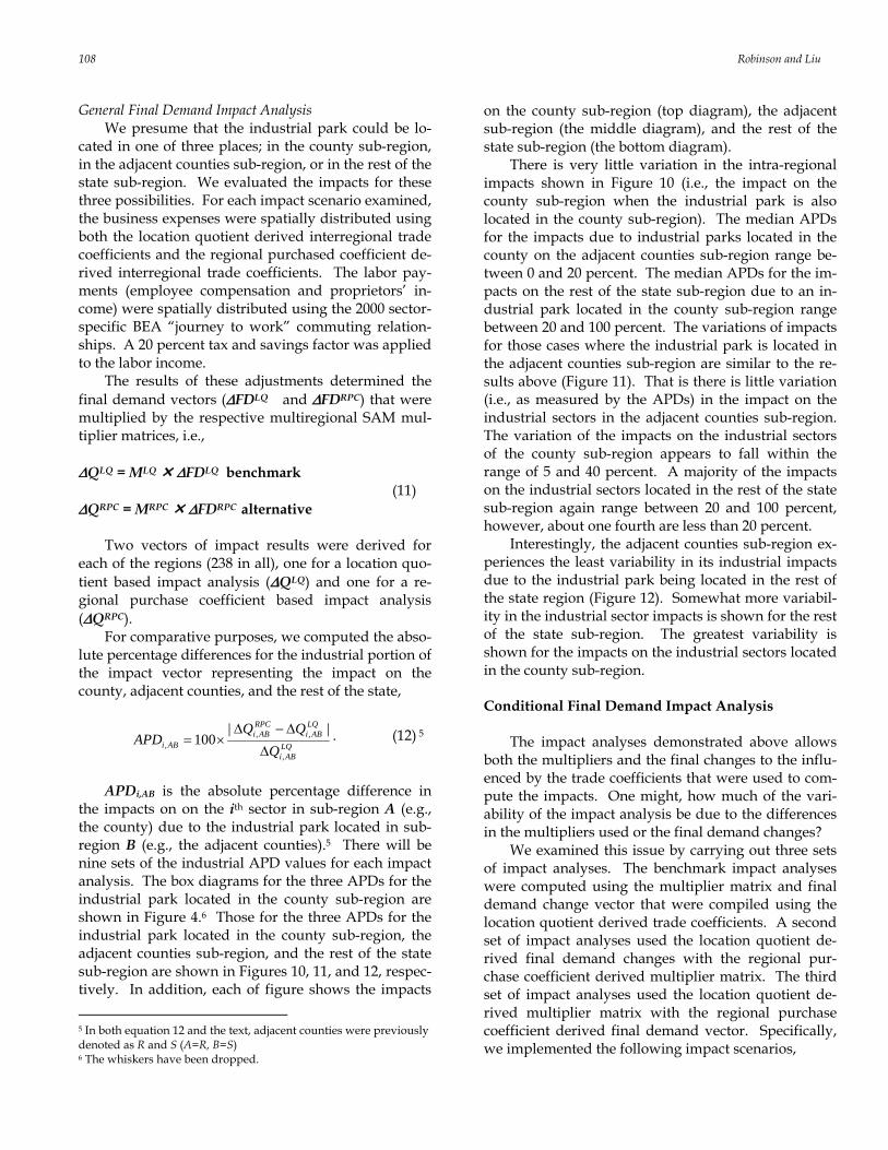
General Final Demand Impact Analysis We presume that the industrial park could be lo-cated in one of three places; in the county sub-region, in the adjacent counties sub-region, or in the rest of the state sub-region. We evaluated the impacts for these three possibilities. For each impact scenario examined, the business expenses were spatially distributed using both the location quotient derived interregional trade coefficients and the regional purchased coefficient de-rived interregional trade coefficients. The labor pay-ments (employee compensation and proprietors’ in-come) were spatially distributed using the 2000 sector-specific BEA “journey to work” commuting relation-ships. A 20 percent tax and savings factor was applied to the labor income. The results of these adjustments determined the final demand vectors (ΔFDLQ and ΔFDRPC) that were multiplied by the respective multiregional SAM mul-tiplier matrices, i.e., ΔQLQ = MLQ ΔFDLQ benchmark (11) ΔQRPC = MRPC ΔFDRPC alternative Two vectors of impact results were derived for each of the regions (238 in all), one for a location quo-tient based impact analysis (ΔQLQ) and one for a re-gional purchase coefficient based impact analysis (ΔQRPC). For comparative purposes, we computed the abso-lute percentage differences for the industrial portion of the impact vector representing the impact on the county, adjacent counties, and the rest of the state,

LQABi

LQABi

RPCABi

ABi QQQ

APD,

,,,

||100

Δ

Δ−Δ×= . (12) 5

APDi,AB is the absolute percentage difference in the impacts on on the ith sector in sub-region A (e.g., the county) due to the industrial park located in sub-region B (e.g., the adjacent counties).5 There will be nine sets of the industrial APD values for each impact analysis. The box diagrams for the three APDs for the industrial park located in the county sub-region are shown in Figure 4.6 Those for the three APDs for the industrial park located in the county sub-region, the adjacent counties sub-region, and the rest of the state sub-region are shown in Figures 10, 11, and 12, respec-tively. In addition, each of figure shows the impacts

5 In both equation 12 and the text, adjacent counties were previously denoted as R and S (A=R, B=S) 6 The whiskers have been dropped.

on the county sub-region (top diagram), the adjacent sub-region (the middle diagram), and the rest of the state sub-region (the bottom diagram). There is very little variation in the intra-regional impacts shown in Figure 10 (i.e., the impact on the county sub-region when the industrial park is also located in the county sub-region). The median APDs for the impacts due to industrial parks located in the county on the adjacent counties sub-region range be-tween 0 and 20 percent. The median APDs for the im-pacts on the rest of the state sub-region due to an in-dustrial park located in the county sub-region range between 20 and 100 percent. The variations of impacts for those cases where the industrial park is located in the adjacent counties sub-region are similar to the re-sults above (Figure 11). That is there is little variation (i.e., as measured by the APDs) in the impact on the industrial sectors in the adjacent counties sub-region. The variation of the impacts on the industrial sectors of the county sub-region appears to fall within the range of 5 and 40 percent. A majority of the impacts on the industrial sectors located in the rest of the state sub-region again range between 20 and 100 percent, however, about one fourth are less than 20 percent. Interestingly, the adjacent counties sub-region ex-periences the least variability in its industrial impacts due to the industrial park being located in the rest of the state region (Figure 12). Somewhat more variabil-ity in the industrial sector impacts is shown for the rest of the state sub-region. The greatest variability is shown for the impacts on the industrial sectors located in the county sub-region. Conditional Final Demand Impact Analysis The impact analyses demonstrated above allows both the multipliers and the final changes to the influ-enced by the trade coefficients that were used to com-pute the impacts. One might, how much of the vari-ability of the impact analysis be due to the differences in the multipliers used or the final demand changes? We examined this issue by carrying out three sets of impact analyses. The benchmark impact analyses were computed using the multiplier matrix and final demand change vector that were compiled using the location quotient derived trade coefficients. A second set of impact analyses used the location quotient de-rived final demand changes with the regional pur-chase coefficient derived multiplier matrix. The third set of impact analyses used the location quotient de-rived multiplier matrix with the regional purchase coefficient derived final demand vector. Specifically, we implemented the following impact scenarios,


Figure 10. General final demand impacts originating in county

Impact on County: Originates in County

0

20

40

60

80

100

120

140

160

IND1

IND3

IND5

IND7

IND9

IND11

IND13

IND15

IND17

IND19

IND21

IND23

IND25

IND27

IND29

IND31

IND33

IND35

IND37

IND39

IND41

IND43

IND45

IND47

IND49

IND51

Abs

olut

e Pe

rcen

tage

Diff

eren

ce (%

)


Impact on Adjacent Counties: Originates in County

0

20

40

60

80

100

120

140

160

IND1

IND3

IND5

IND7

IND9

IND11

IND13

IND15

IND17

IND19

IND21

IND23

IND25

IND27

IND29

IND31

IND33

IND35

IND37

IND39

IND41

IND43

IND45

IND47

IND49

IND51

Abs

olut

e Pe

rcen

tage

Diff

eren

ce (%

)


Impact on Rest of State: Originates in County

0

20

40

60

80

100

120

140

160

IND1

IND3

IND5

IND7

IND9

IND11

IND13

IND15

IND17

IND19

IND21

IND23

IND25

IND27

IND29

IND31

IND33

IND35

IND37

IND39

IND41

IND43

IND45

IND47

IND49

IND51

Abs

olut

e Pe

rcen

tage

Diff

eren

ce (%

)



Figure 11. General final demand impacts originating in adjacent counties

Impact on County: Originates in Adjacent Counties

0

20

40

60

80

100

120

140

160

IND1

IND3

IND5

IND7

IND9

IND11

IND13

IND15

IND17

IND19

IND21

IND23

IND25

IND27

IND29

IND31

IND33

IND35

IND37

IND39

IND41

IND43

IND45

IND47

IND49

IND51

Abs

olut

e Pe

rcen

tage

Diff

eren

ce (%

)


Impact on Adjacent Counties: Originates in Adjacent Counties

0

20

40

60

80

100

120

140

160

IND1

IND3

IND5

IND7

IND9

IND11

IND13

IND15

IND17

IND19

IND21

IND23

IND25

IND27

IND29

IND31

IND33

IND35

IND37

IND39

IND41

IND43

IND45

IND47

IND49

IND51

Abs

olut

e Pe

rcen

tage

Diff

eren

ce (%

)


Impact on Rest of State: Originates in Adjacent Counties

0

20

40

60

80

100

120

140

160

IND1

IND3

IND5

IND7

IND9

IND11

IND13

IND15

IND17

IND19

IND21

IND23

IND25

IND27

IND29

IND31

IND33

IND35

IND37

IND39

IND41

IND43

IND45

IND47

IND49

IND51

Abs

olut

e Pe

rcen

tage

Diff

eren

ce (%

)



Figure 12. General final demand impacts originating in rest of the state

Impact on County: Originates in Rest of State

0

20

40

60

80

100

120

140

160

IND1

IND3

IND5

IND7

IND9

IND11

IND13

IND15

IND17

IND19

IND21

IND23

IND25

IND27

IND29

IND31

IND33

IND35

IND37

IND39

IND41

IND43

IND45

IND47

IND49

IND51

Abs

olut

e Pe

rcen

tage

Diff

eren

ce (%

)


Impact on Adjacent Counties: Originates in Rest of State

0

20

40

60

80

100

120

140

160

IND1

IND3

IND5

IND7

IND9

IND11

IND13

IND15

IND17

IND19

IND21

IND23

IND25

IND27

IND29

IND31

IND33

IND35

IND37

IND39

IND41

IND43

IND45

IND47

IND49

IND51

Abs

olut

e Pe

rcen

tage

Diff

eren

ce (%

)


Impact on Rest of State: Originates in Rest of States

0

20

40

60

80

100

120

140

160

IND1

IND3

IND5

IND7

IND9

IND11

IND13

IND15

IND17

IND19

IND21

IND23

IND25

IND27

IND29

IND31

IND33

IND35

IND37

IND39

IND41

IND43

IND45

IND47

IND49

IND51

Abs

olut

e Pe

rcen

tage

Diff

eren

ce (%

)



LQLQLQ FDMQ Δ×=Δ benchmark

RPCRPCRPC FDMQ Δ×=Δ 0 alternative 0

(13) LQRPCRPC FDMQ Δ×=Δ 1 alternative 1

RPCLQRPC FDMQ Δ×=Δ 2 alternative 2

Three sets of STPDs values for each of the 238 area SAM models were computed using the impact analy-ses in equation [13],

LQAi

i

LQAi

RPCAi

A Q

QQSTPD

,

,0,

0

||100

Δ

Δ−Δ×=∑ alternative 0

LQAi

i

LQAi

RPCAi

A Q

QQSTPD

,

,1,

1

||100

Δ

Δ−Δ×=∑

alternative 1 (14)

LQAi

i

LQAi

RPCAi

A Q

QQSTPD

,

,2,

2

||100

Δ

Δ−Δ×=∑ alternative 2

Comparing the benchmark and alternative 0 im-pact analyses provides the total variation in differ-ences in impacts from both the multipliers and final demand. This represents the variability due to differ-ences in the way that both the multipliers and final demand changes were estimated. Alternatives 1 and 2 provide a decomposition of the total variation. For example, if the benchmark and alternative 1 impact analyses are compared, we can see the effects of the multipliers on the impact analysis. Also, the effects on the impact analysis due to the final demand assump-tion are shown by comparing the benchmark and al-ternative 2 impact analyses. Figure 13 shows the box diagrams for the STPDs of the alternatives 0, 1, and 2. Comparing the box dia-grams for STPD alternatives 1 and 2 clearly shows that most of the variability in the impact results is due to the affects of how the trade flows affected the multi-plier estimates.

LQ vs RPC Method of Estimating Trade Flows:Affect of Final Demand Imapcts

0

10

20

30

40

50

60

70

Cnt

y/C

nty

Adj

/Cnt

yR

oS/C

nty

Tota

l Cnt

yC

nty/

Adj

Adj

/Adj

RoS

/Adj

Tota

l Adj

Cnt

y/R

oSA

dj/R

oSR

oS/R

oSTo

tal R

oSC

nty/

Cnt

yA

dj/C

nty

RoS

/Cnt

yTo

tal C

nty

Cnt

y/A

djA

dj/A

djR

oS/A

djTo

tal A

djC

nty/

RoS

Adj

/RoS

RoS

/RoS

Tota

l RoS

Cnt

y/C

nty

Adj

/Cnt

yR

oS/C

nty

Tota

l Cnt

yC

nty/

Adj

Adj

/Adj

RoS

/Adj

Tota

l Adj

Cnt

y/R

oSA

dj/R

oSR

oS/R

oSTo

tal R

oS

Chg Mult/Chg FD Chg Mult/Hold FD Hold Mult/Chg FD

Stan

dard

ized

Tot

al P

erce

ntag

e D

iffer

ence

(%)


Figure 13. Variability of final demand impact estimates based on two techniques of deriving interre-

gional commodity trade flows


5. Conclusion and Recommendations SAM models provide regional economic devel-opment professionals with invaluable quantitative economic impact evaluation tools. These models per-mit assessments of different important policy deci-sions over an entire economic system using the effects of important economic aggregates and agents. IM-PLAN provides social accounting data in a convenient format that can be used to construct single region in-put-output and SAM models. The availability of the Bureau of Transportation Statistics’ Commodity Flow Survey (CFS) and BEA’s “journey-to-work” commuter data are permitting economic impact modelers to ex-tend IMPLAN’s single regional SAM models to mul-tiregional formats. Unfortunately, the Bureau of Transportation Statistics has not extended their CFS data to provide an official source for state-to-state commodity transport flows for public release and use. Jackson, et al (2004) describe methods of estimating trade flows using data from the commodity flow sur-vey. Little research exists concerning the creation of multiregional models at geographic scales lower than states, especially the roll that interregional trade plays. This paper evaluates the effects of using two interre-gional trade flow estimating procedures on multire-gional SAM multipliers. One uses a variation of loca-tion quotient to estimate domestic exports. The other uses the regional purchase coefficients that IMPLAN produces to estimate domestic imports. The estimated domestic imports and exports for both sets of trade flow estimates are balanced to fit within IMPLAN’s accounting framework. The techniques employed in this paper are applied to 238, 3-region multiregional SAM models. The results presented in this paper clearly demon-strate that the methods used to estimate the interre-gional trade flows can substantially affect both the interregional multipliers and the estimated impacts that are derived from multiregional SAM models. These results should be quite perplexing to the re-gional economic impact practitioners because the trade flow matrices necessary to compile multiregional SAM models have to be estimated in some way. The purpose of this paper was simply to address the issue of how much difference the choice of estimating method makes. Recently, inter-county trade flow estimates for each of the 509 commodities and services in the IM-PLAN system have been constructed by Lindall et al. (2005). These estimates will make constructing mul-tiregional SAM models feasible for almost any re-

gional configuration a user may desire. One question is should the current regional purchase coefficients be the underlying accounting basis for the intraregional trade assumptions? Or, should the estimated trade flows provide not only the interregional trade assump-tions between regions but also the intraregional trade assumptions? Acknowledgement

The authors would like to thank Thomas G. John-son of the University of Missouri—Columbia for help-ful discussions, advice, and support in the develop-ment of this paper. An earlier version of this paper was presented at the 2005 MCRSA/SRSA Meetings in Arlington, VA on April 7-9. References Hewings, Geoffrey J.D.; Yasuhide Okuyama; and Mi-

chael Sonis. 2001. “Economic Interdependence within the Chicago Metropolitan Area: A Miya-zawa Analysis.” Journal of Regional Science, 41, pp. 195-217.

Holland, David and Peter Wyeth. 1993. “SAM Multi-pliers: Their Interpretation and Relationship to In-put-Output Multipliers.” Edited by Daniel M. Otto and Thomas G. Johnson in Microcomputer-Based Input-Output Modeling: Applications to Economic Development. Boulder, CO: Westview Press, pp. 181-197.

Isserman, Andrew. 1977. “The Location Quotient Ap-proach to Estimating Regional Economic Impact.” Journal of American Institute of Planners, January.

Jackson, Randall W. 2002. Constructing US Interregional SAMs from IMPLAN Data: Issues and Methods. 2002-14. Morgantown, WV: Regional Research Institute, West Virginia University.

Jackson, Randall W.; Walter R. Schwarm; Yasuide Okuyama; and Samia Islam. 2004. A Method for Constructing Commodity by Industry Flow Matrices. Research Paper 2004-5. Morgantown, WV: Re-gional Research Institute, West Virginia Univer-sity.

Lindall, Scott; Olson, Doug; and Alward, Greg. 2005. Multiregional Models: The IMPLAN National Trade Flows Model. Prepared for the 2005 MCRSA/SRSA Meetings in Arlington VA April 7-9.

King, Benjamin B. 1985. “What is a SAM?” Edited by Graham Pyatt and Jefferey I. Round in Social Ac-counting Matrices: A Basis for Planning. Washing-ton, DC: The World Bank, 17-51.


Miller, Ronald E. and Peter D. Blair. 1982. State-Level Technology in the U.S. Multiregional Input-Output Model. Working Papers in Regional Science and Transportation, No. 65. Philadelphia, PA: Univer-sity of Pennsylvania.

Minnesota IMPLAN Group (MIG), Inc. 1998. Elements of the Social Accounting Matrix. MIG IMPLAN Technical Report TR-98002. Stillwater, MN: Min-nesota IMPLAN Group, Inc.

Minnesota IMPLAN Group, Inc. (MIG). 2000. IMPLAN Professional, Version 2.0: Social Accounting & Impact Analysis Software, 2nd Edition. Stillwater, MN: Min-nesota IMPLAN Group, Inc. (June).

Peterson, William C. and Roger J. Beck. 2001. “Central Places, Trade Flows, and Input-Output Analysis: Another Look at Estimating Regional Purchase Coefficients.” Paper presented at the annual meet-ing of the Southern Regional Science Association on April 5-7 in Asutin, TX.

Pyatt, Graham and Jefferey I. Round. 1985. “Regional Accounts in a SAM Framework.” Edited by Gra-ham Pyatt and Jefferey I. Round in Social Account-ing Matrices: A Basis for Planning. Washington, DC: The World Bank, pp. 84-95.

Robinson, Dennis P. and Thomas G. Johnson. 2005. A User Guide to the Socio-Economic Benefits Assessment System: A Rural Business-Cooperative Services As-sessment Tool for Economic Development. Columbia, MO: Community Policy Analysis Center (CPAC), University of Missouri-Columbia (January).

Round, Jeffery. 2003. “Social Accounting Matrices and SAM-Based Multiplier Analysis. Edited by Fran-cois Bourguignon and Luiz A. Pereira da Silva in Evaluating the Poverty and Distributional Impact of Economic Policies (Techniques and Tools). Washing-ton, DC: The World Bank, in draft (March).

Southworth, Frank and Bruce E. Peterson. 2000. “In-termodal and International Freight Network Mod-eling.” Transportation Research Part C, 8, pp. 147-166.

Tukey, John W. 1977. Exploratory Data Analysis, First Edition. Reading, MA: Addison-Wesley Publishing Co.

the effects of interregional trade flow estimating … · 2017-09-11 · the effects of...

Documents