THE EFFECTS OF LOW LEVEL TURBIDITY

ON

FISH AND THEIR HABITAT

James P. Reed John M. Miller David F. Pence Barbara Schaich

Department of Zoology North Carolina State University

Raleigh, NC 27650

The work upon which this publication is based was supported in part by funds provided by the U. S. Department of the Interior, Washington D. C. through the Water Resources Research Institute of The University of North Carolina as authorized by the Water Research and Development Act of 1978. The work was also supported by Agricultural Research Services at North Carolina State University.

Project No. B-132-NC Agreement No 14-34-0001-0237

ACKNOWLEDGMENTS

The authors are indebted to and gratefully acknowledge

the assistance rendered by the following individuals: A.

Dean Goodnight, Sue Ann Colvin, and Stefane Bowles were

instrumental in collecting, processing and analyzing samples

of plant and animal abundance. Dr. George Barthalamus, B.

Mac Currin, S. Dianne Moody, and Melanie Shaefer assisted in

manipulation and maintainence of enclosures and equipment.

Dr. Edward Wiser and Phil Harris of the NCSU Department of

Agricultural Engineering aided in the implementation of

remote data acquisition systems, and in system interfacing

'with and data transfer to the mainframe computers. Drs.

Howard Kerby and Melvin Huish of the NCSU U.S. Cooperative

Fisheries Unit were most generous with their boats and

sampling equipment.

ABSTRACT

The effects of low level turbidity on fish habitat were

investigated from July 1980 to September 1982 in a pond near

Raleigh, NC. Three levels of turbidity were maintained in

polyvinylchloride curtain enclosures with open bottoms each 2 of which enclosed 260-400 m and had a maximum depth of 2

m. Turbidity levels in the pond routinely ranged from 6 to

50 NTU turbidity units with peaks associated with blue-green

algal blooms in excess of 120 NTU. The turbid enclosure was

maintained between 7 and 45 NTU, the cleared enclosure was maintained between 2 and 12 NTU and the untreated control

was between 4 and 18 NTU. Total suspended solids, TSS,

explained 68% of the variability associated with turbidity:

a 10 mg/l increase in TSS increased turbidity 6 NTU units.

Turbidity affected light penetration as determined by secchi

depth. In the pond and turbid enclosure the secchi depth

represented the 30% light level whereas in the cleared

enclosure the secchi depth was equivalent to the generally

accepted 15% light level, A 10 NTU increase in turbidity

resulted in a 0.6 m-I increase in the light extinction

coefficient. As light penetration decreases, the light

energy is transformed into heat over a shorter distance and

higher epilimnetic temperatures may result. This theory was

tested using the above relationships to develop a model,

which included the effects of backscatter, to predict

epilimnetic temperature changes as a function of turbidity. It was found that as the turbidity increased and/or depth of

the epilimnion decreased, the magnitude of the temperature

change increased. This was validated by field observations

for an epilimnion depth of 0.25 m. In this case,

temperatures in the turbid enclosure (28 NTU) were 2-5*~

higher than the cleared enclosure (14 NTU). However, at the 'normal1 epilimnion depth of lm, large increases in

turbidity resulted in only small temperature increases.

Turbidity also had a direct effect on the fish's physical

habitat: a reduction from 12 NTU to 6 NTU enabled submerged

macrophytes, due to the increased available light, to

colonize deeper waters. This increase in plant biomass

would result in increased invertebrate prey and therefore

higher fish production.

TABLE OF CONTENTS

Page

..................................... ACKNOWLEDGMENTS ii

ABSTRACT ............................................ iii

LIST OF FIGURES .................................... vi

...................................... LIST OF TABLES v i i

SUMMARY AND CONCLUSIONS ............................. v i i i

RECOMMENDATIONS ..................................... i x

........................................ INTRODUCTION 1

METHODS ............................................. 5

RESULTS ............................................. 10

.......................................... DISCUSSION 28

LITERATURE CITED..................................... 34

LIST OF FIGURES

NUMBER DESCRIPTION

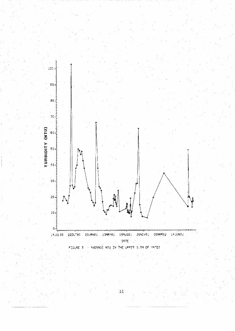
1 Average turbidity in the upper

of Yates Pond ...................................

2 Average suspended solids in the upper 0.5 m

of Yates Pond ...................................

3 Extinction coefficient for Yates Pond vs time ...

4 Average temperature in the upper 0.5 m of Yates Pond ...................................

5 Temperature vs depth by subponds for Sept. 1982 .

6 Temperature vs depth by subponds for Aug. 1982 ..

7 Dissolved oxygen vs time for Yates Pond .........

8 Average chlorophyll - a in the upper 0.5 m

Yates Pond ...................................

PAGE

LIST OF TABLES

NUMBER DESCRIPTION PAGE

Seasonal averages of turbidity, chlorophyll - a, phaeo-pigments, total suspended solids, percent

organic matter, secchi depth, one percent light

level and extinction coefficient .................. 10

Relationships between turbidity, NTU and total

suspended solids .................................. 13

Relationships between TSS, NTU and extinction

coefficients, Nt .................................. 15

Change in bottom area coverage of Chara beds

in relation to changes in turbidity in 1981 ....... 21

Net ecosystem production values for Yates and

subponds in 1981 and 1982 ......................... 21

Water quality parameters a blue-green algal bloom

be£ ore, in 1981

during and after .................. 23

SUMMARY AND CONCLUSIONS

An investigation of the effects of low levels of

turbidities on fish habitat was conducted from June 1980 to

September 1982 in Yates Pond, Wake County, NC. This study

investigated the major parameters which were affected by

turbidity and influenced fish habitat such as temperature,

dissolved oxygen and plant biomass. A mathematical model of

the effects of turbidity on temperature was also developed.

We observed in the field and predicted from the model

that under low wind conditions, turbidity was responsible

for increasing the water temperature by as much as 4'~

within two days. This increased temperature increases the

metabolic cost of fish living in this zone and may exacerbate oxygen depletion in the hypolimnion which would

then preclude its use by fish as well as their prey. High

levels of turbidity were correlated to restricted

development of submerged plants which in addition were

probably responsible for reduced dissolved oxygen levels.

In Yates Pond, the sources of turbidity were clays and

silts as well as blue-green algae. The highest turbidity

levels observed were due to blue-greens algal blooms. These

blooms lasted for two to three weeks during which time the

water column was supersaturated with oxygen. After the

algae died, though, the concentration of oxygen in the water

was so low (3-4 mg 02/1) as to be stressful to fish.

In summary, low level increases in turbidity negatively

impact the fish's physical habitat through increases in

temperature and decreases in submerged plants which would

potentially reduce epiphytic prey as well as dissolved oxygen levels.

RECOMMENDATIONS

Ecological benefits of turbidity control to fish

habitat must be considered on a case-by-case basis.

Turbidity control should be dealt with as part of a total

water management plan. In general, a decrease in turbidity

will result in an increase in primary production due to the

increased available light. This increased primary

production results in an increase in

which in turn are consumed by fish.

invertebrate grazers

Whether the increase in primary

phytoplankton or macrophytes depends production is due to

primarily on water depth, which affects light penetration, 'seed1 source for

the plants, and nutrient availability. Under high nutrient loading conditions, phytoplankton biomass may increase to

high levels which could result in low dissolved oxygen at

night or anoxic conditions when the population dies. Such

rapid changes in dissolved oxygen are not generally

associated with macrophytes. In fact, if macrophytes are

growing below the thermocline, anoxic bottom waters may not

occur. Crowder (1982) showed that fish do well at

intermediate macrophyte densities due to the increases in

habitat structure and the associated prey, but do less well

at either high or low densities. This is of concern in

shallow ponds and lakes and on the margins of deeper

reservoirs because macrophytes are generally found in waters

less than 1 m deep.

When water temperatures are higher than 30°c,

measures should be taken to ensure that rapid turbidity

increases do not occur. Under certain environmental

conditions, i. e. no wind, shallow epilimnion, anoxic bottom

waters, and a turbidity increase of 60 NTU, fish are likely

to die because they are unable to contend with the

oxygenated but lethal temperatures of the surface waters and

the cooler but anoxic bottom waters. We have no estimates

of the frequency of occurrence of this set of circumstances.

However, we did observe a fish kill in Yates Pond for just

such reasons in 1977.

In general a water management program for an area with

high nutrient loading that deals with turbidity abatement I alone is likely to lead to a decrease in environmental

quality unless the nutrients are decreased as well.

INTRODUCTION

Effects of suspended solids or turbidity have been

found on nearly every trophic level in aquatic ecosystems

Fig. 1 . King and Ball's (1964) study of the effects of

highway construction found a two-fold increase in inorganic

sediment load reduced by half the primary production of

streams (from 269 to 124 mg C m-2day-1 1 . Strawn (1961)

working in Florida, showed that turbidity was partly

responsible for restricted zones of submerged macrophytes

and suggested that an important food source for fishes had

been reduced. Similarly, Hart and Fuller (1972) found that

persistent high turbidity levels limited the development of

macrophytes in the Patuxent River. Williams (1966) showed a

reduction in zooplankton associated with increased suspended

solids. Hubbs (1940) found evidence of reduced eye size, increases in other sensory organs, changes in body form,

color and fin development among fishes inhabiting turbid

waters.

Effects of suspended solids or turbidity on fishes can

be categorized into direct and indirect effects. Examples of direct effects include the following: Green sunfish

exhibited a stress response to turbidity (20,000 JTU)

(Wallen 1951); green sunfish increased ventilation rates

with bentonite suspension levels of about 7500 mg/l (Horkel and Pearson 1976); at much higher levels suspended solids levels also caused gill damage and suffocation in fishes (Ellis 1944); and Wallen also listed lethal

suspended solids levels for 14 warm-water species of fish as

ranging from 38,250 to 222,000 mg/l . With few exceptions

fishes show little direct damage except by very high levels

of suspended solids.

Indirect effects on behavior of fishes occur at

considerably lower levels. The reactive distance of

bluegills to zooplankton prey was reduced at turbidities as

low as 6.25 JTU (Vineyard and OIBrien 1976). Similarly,

Gardner (1981) found the feeding rate of bluegill on

Daphnia was inversely proportional to turbidity. At the

highest turbidity tested (190 JTU) the feeding was 54% of

the control.

Additional indirect effects include blockage of

spawning migrations by striped bass which occurred at 300

mg/l suspended solids, ss, (Radtke and Turner 1967) and

reduced feeding by trout at 35 mg/l ss (Bachmann 1959). The

vertical distribution of larval lake herring changed when

exposed to turbidity levels of 26-28 FTU (about 18 mg/l

ss)(Swenson and Matson 1976). Activity was reduced and

social hierarchies of largemouth bass and green sunfish were

disturbed at turbidities of 4-16 JTU (Hemistra et al. 1969).

More general effects include reduced fish populations

and reduced fishing success and effort (Buck 1956). In his

study primary productivity was 12.8 times higher in clear than turbid (100 mg/l ss) ponds and the former supported 5.5

times more fish.

Any increase in turbidity, however, affects light

penetration and therefore, can affect primary production,

hence oxygen concentration, and temperature. These, in turn, can have sub-lethal effects on fishes,

Doudoroff and Shumway (1970) reviewed the literature on

dissolved oxygen requirements of fishes. Among the more

important findings pertinent to the discussion were those of

Hoglund (1961) who showed increased fish activity in oxygen deficient water. Whitmore et al. (1960) found avoidance of

oxygen concentrations of 3 mg/l and 4.5 mg/l by largemouth

bass and bluegill, respectively. They further argued that, unlike Hoglundls suggestion of low oxygen "releasing

stimulusw to higher activity, fish in their experiments

exhibited a "directed response" away from low oxygen. Dunst

(1969) found largemouth bass could not survive in the low

oxygen ((5.0 mg 02/1) hypolimnion of many Wisconsin lakes in summer. Tolerance of low oxygen, and perhaps avoidance,

is affected by thermal stress (Moss and Scott 1961).

Hutchinson (1976) found the converse, that is, reduced

temperature tolerance in oxygen-stressed fish.

The subject of temperature tolerance of fishes has

received considerably more attention than oxygen tolerance.

Recently, most research has been directed at sub-lethal

effects of temperature on fishes. Doudoroff (1969) found

the maintenance ration of largemouth bass increased from

0.5% of body weight day to 2.0% with an increase in

temperature from 10 to 15Oc. Sylvester (1972) found that

thermally stressed sockeye salmon were more vulnerable to

predation. Coutant et al. (1974) reported similar findings

for young largemouth bass and channel catfish. Coutant and

Cox (1976) found the temperature for maximum growth to be 26

and 27OC for small and large largemouth bass,

respectively. Growth was thus depressed well before the

incipient lethal temperature (about 36.5'~) was reached.

They suggested 31.3'~ as an upper limiting temperature.

Plumb (1973) found heat-stressed channel catfish to be more

susceptible to disease, and Swallow (1968) found increased

mortality among fish embryos exposed to higher incubation temperatures.

The preferred temperature and temperature avoidance

behavior of fishes generally reflects these sub-lethal

temperatures. Peterson and Schutsky (1976) found bluegill

acclimated to 27.0'~ preferred a temperature of 31.7'~ and avoided 33.s°C which is below their upper lethal

limit. Neil1 and Magnuson (1974) investigated the preferred

temperature of 11 species of fish in Wisconsin and also

3

found

below

that these fish avoided temperatures well above and

their lower and upper let.hal limits, respectively.

Conclusions possible from the literature are: 1) fish

generally avoid conditions well inside their lethal limits

of both temperature and oxygen; and 2) sub-optimal growth

(or health) probably occurs when fish are forced to live

outside their preferred ranges of oxygen and temperature.

In nature, and especially in stratified small turbid

lakes, it is likely that the habitat (living space) of

fishes in summer is restricted to an intermediate stratum

between avoided high temperature above and avoided low

oxygen below.

In eutrophic lakes, fish are often excluded from the

hypolimnion by the low oxygen levels in summer (Dunst 1969).

In turbid lakes, fish may also be thermally excluded from

surface layers. An extreme example occurred in Yates Pond,

NC, during fall 1977. Defining the living space of fish as

water below 310c and having more than 4.5 mg/l 02, this was a layer between 0.2 and 1.5 m on 29 July. During the

ensuing 14 days, this living space shrunk; on 8 August it

was between 0.6 and 0.8 m. On 12 August the two boundaries

converged and on the same day, a fish kill of an estimated

500 kg occurred.

This study documents the indirect effects of low levels of turbidity on factors that influence fish habitat such as

temperature and dissolved oxygen as well as chlorophyll a and macrophyte distribution. A companion report is

currently in preparation that will describe the direct

effects of turbidity on fish feeding and their prey.

In . c m r l 0 a, -4 c, w

c, b r a 0 Id a 9

a, k .Ll 5

r'l

0

(I) C 0

C Id C E c,

0 m A Id 3 a

(I) h v, c, V)

suspended material removed by a chemical flocculating agent

and one served as a control. Between experimental runs,

then enclosures were pulled onto shore and scrubbed in order

to remove periphyton growth.

Turbidity manipulations

Suspended sediments were removed from the enclosures

using alum (aluminum sulfate) and calcium hydroxide (Boyd

1979). In 1981 approximately 22 kg of alum to 3 kg of

Ca(OHI2 per enclosure was added in the following manner: 4.4 kg alum was mixed with pond water in a 100 1 plastic

container. In a second container, 600 g Ca(OH12 was mixed

with pond water. Contents of both were added simultaneously

from a boat. This procedure was repeated five times.

Settling of suspended solids began almost immediately with

equilibrium levels reached within 24 hours. In 1982, because

of the reduced size of the enclosures, 9 kg alum and 1.2 kg

of Ca(OH12 were used per enclosure. The diluted chemicals were sprayed from shore from the containers using a submersible pump. If during the experiment, turbidity

increased, an additional 4.5 kg alum and 600 g Ca(OHI2

were added.

In 1981 turbidity in enclosures was enhanced by the

addition of benthic mud sieved through 3 3 5 micrometer

plankton nets. Approximately 90 1 of mud were added in

early morning three times per week. In 1982, we used

commercially available bentonite. On day one 18 kg of

bentonite was mixed with well water in a 100 1 container and

sprayed out over the enclosure using a submersible pump.

Then on every other day an additional 4 . 5 to 9.0 kg were

added in a similar manner.

Field sampling

Yates pond was sampled weekly during 1980 and 1981.

After late 1981 samples were taken monthly through early

1982. The subponds were sampled intensively, sometimes as

often as twice a day for several days in a row.

Water samples were taken from surface to bottom at O.5m

intervals using a Van Dorn sampler. Three replicates were

taken at 0.5m depth, single samples at other depths. The

samples were placed in plastic bottles and processed in the

lab within 3 hours.

Temperature, dissolved oxygen and light

Water temperatures were measured at depths 0 m

(surface), 0.02 m, 0.03 m, and 0.25 m to the bottom at 0.25m

intervals using a digital thermometer (Bailey Instruments

BAT-81 equipped with thermocouple probes. In 1982

temperatures were taken with a YSI Model 54M Oxygen Meter

equipped with a thermistor.

Dissolved oxygen was measured in the field with a YSI

oxygen meter from the surface (0 m) to the bottom at 0.25 m

intervals.

Underwater intensities of photosynthetically active

radiation (PAR) in the 400-700 nanometer waveband was

measured using a Li-Cor LI-192s Underwater Quantum Sensor

and the Li-Cor LI-18524 Quantum meter/ Radiometer/

Photometer. Omnidirectional PAR in the same range was

measured using a Li-Cor LI-193s Spherical Quantum Sensor.

Turbidity measurement

Turbidity was measured with a Turner Model I11

fluorometer (Turner Instruments, Inc.) adapted for

nephelometry. In 1980-81, the instrument was equipped with

Turner filter # 5-60 (430-450 nm) in the primary slot and neutral density filters equivalent to 0.5% transmittance in

the secondary slot. All readings were made with the

sensitivity scale set to ' 3 ~ ' . Calibration curves were

produced using standard formazin mixtures (APHA et.

a1.,1975) and measuring their turbidities in a square cuvette.

In March, 1982 the filters were changed because the

fluorometer had been modified to measure chlorophyll. The

filters used were Turner filter # 10-053 (or Kodak Wratten color specification 16) in the primary slot and 3%

transmittance Neutral Density filters in the secondary slot.

The machine required frequent rezeroing after this modification.

Determination of total suspended solids and organic fraction

In the lab, the water samples were shaken and 50 ml - 1,000 ml were filtered through prewashed, preweighed Whatman glass fiber filter (GF/C) with a 1.2 micrometer pore

size. Filters were dried for 20-24 hours at 5 5 O ~ to

determine total suspended solids, TSS. They were then

weighed, combusted for 1 hour combustion at 550°c, and

reweighed to determine the percent organic fraction.

Determination of chlorophyll 5

Water samples were shaken and 25 ml to 100 ml were

filtered with 22 cm of Hg vacuum through a 47 mm diameter,

0.45 micrometer pore, Millipore acetate filter. When

approximately 10-15 ml of the sample remained to be

filtered, 1-2 ml of a saturated magnesium carbonate

(MgC03) solution was added to prevent chlorophyll deterioration. Two to three replicate filters were prepared

from each field sample. The filters were folded, placed in

vials, enclosed in light-tight boxes and frozen.

Chlorophyll was extracted in the freezer with 10 ml of 90%

acetone for 20-24 hours. The contents of the vial were

centrifuged, diluted and measured in a Turner Model I11

fluorometer equipped as in Lorenzen (1966). Phaeo-pigments

were determined by acidification.

Net ecosystem production

Daily changes in oxygen in free water were used to

calculate net ecosystem production, NEP:

NEP=(O2 change in epilimnion)*(depth of epilmnion) *(proportion of solar day)

where the proportion of the solar day is a factor that

adjusts for change in solar energy throughout the day.

Changes in planktonic oxygen production were measured using 300 ml glass bottles.

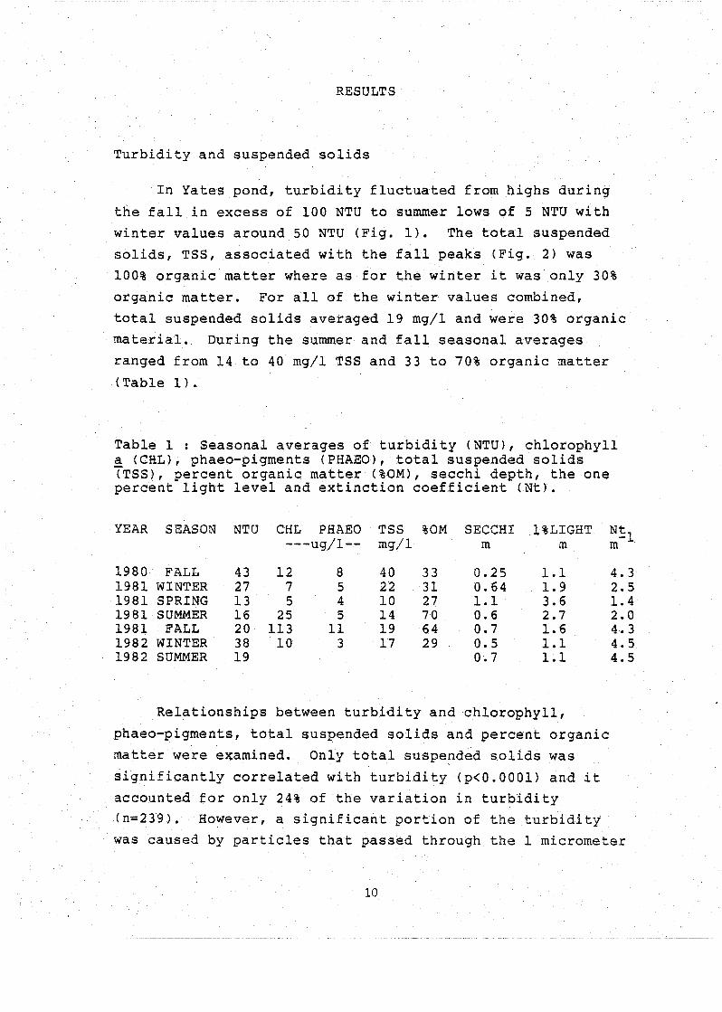
RESULTS

Turbidity and suspended solids

In Yates pond, turbidity fluctuated from highs during

the fall in excess of 100 NTU to summer lows of 5 NTU with

winter values around 50 NTU (Fig. 1). The total suspended

solids, TSS, associated with the fall peaks (Fig. 2) was

100% organic matter where as for the winter it was only 30%

organic matter. For all of the winter values combined,

total suspended solids averaged 19 mg/l and were 30% organic

material. During the summer and fall seasonal averages

ranged from 14 to 40 mg/l TSS and 33 to 70% organic matter

(Table 1).

Table 1 : Seasonal averages of turbidity (NTU), chlorophyll a (CHL), phaeo-pigments (PHAEO), total suspended solids - (TSS), percent organic matter (%OM), secchi depth, the one percent light level and extinction coefficient (Nt).

YEAR SEASON NTU CHL PHAEO TSS %OM SECCHI l%LIGHT ---ug/l-- mg/l m m

1980 FALL 43 12 8 40 33 0.25 1.1 1981 WINTER 27 7 5 22 31 0.64 1.9 1981 SPRING 13 5 4 10 27 1.1 3.6 1981 SUMMER 16 25 5 14 70 0.6 2.7 1981 FALL 20 113 11 19 64 0.7 1.6 1982 WINTER 38 10 3 17 29 0.5 1.1 1982 SUMMER 19 0.7 1.1

Relationships between turbidity and chlorophyll,

phaeo-pigments, total suspended solids and percent organic

matter were examined. Only total suspended solids was

significantly correlated with turbidity (p<0.0001) and it

accounted for only 24% of the variation in turbidity

(n=239). However, a significant portion of the turbidity

was caused by particles that passed through the 1 micrometer

a -4 a, rn a -4 C C C rl

5 rd c, a, -4

N C d P k lZ c V r l

w d P O C ~ O t n f - l 4 J c , c, -4 a c t r l k u - r m m a, C -4 -4 . o a a

c U ~ I - + - ( C O Q ) -4 a c, a t n w r n a , a r n c d w r l a , a , k a a , a a k a , O C rd k 3 u c , ~ - r a , o a

- - C U C C +' a, 0 -4 N -4

4J C a, - ( d l 3

c , ~ a r m c U \ r l c , c , c TJ' c -4 a , h G c , r l 0 - 4 4 J a l X U -4 +J

w w m a O a , W C E

c , w a , - 4 3 C Q ) + ' c , 0 - 4 0 C W

r-4 3 U - d a ,

from 1.1 m to 3.6 m. Based on 66 observations that spanned

two years, we estimated that the depth at which the secchi

disk disappears corresponds to the 30% light level.

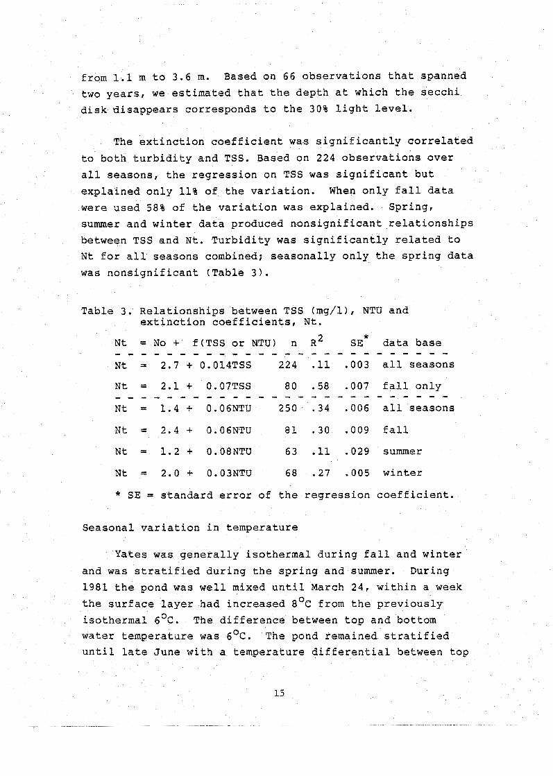
The extinction coefficient was significantly correlated

to both turbidity and TSS. Based on 224 observations over

all seasons, the regression on TSS was significant but

explained only 11% of the variation. When only fall data

were used 58% of the variation was explained. Spring,

summer and winter data produced nonsignificant relationships

between TSS and Nt. Turbidity was significantly related to

Nt for all seasons combined; seasonally only the spring data

was nonsignificant (Table 3).

Table 3. Relationships between TSS (mg/l), NTU and extinction coefficients, Nt.

Nt = N o + f(TSSorNTU1 n R SE* data base . . . . . . . . . . . . . . . . . . . . . . . . . . Nt = 2.7 + 0.014TSS 224 .11 .003 all seasons

Nt = 2.1 + 0.07TSS 80 .58 .007 fall only . . . . . . . . . . . . . . . . . . . . . . . . . . Nt = 1.4 + 0.06NTU 250 .34 .006 all seasons

Nt = 2.4 + 0.06NTU 81 .30 .009 fall

Nt = 1.2 + 0.08NTU 63 .11 .029 summer

Nt = 2.0 + 0.03NTU 68 .27 .005 winter

* SE = standard error of the regression coefficient.

Seasonal variation in temperature

Yates was generally isothermal during fall and winter

and was stratified during the spring and summer. ~uring

1981 the pond was well mixed until March 24, within a week

the surface layer had increased 8'~ from the previously

isothermal 6'~. The difference between top and bottom

water temperature was 6'~. The pond remained stratified

until late June with a temperature differential between top

and bottom, a 2 m distance, of 8-9'~. The epilimnion was

0.75 m deep. It restratified and remained that way until

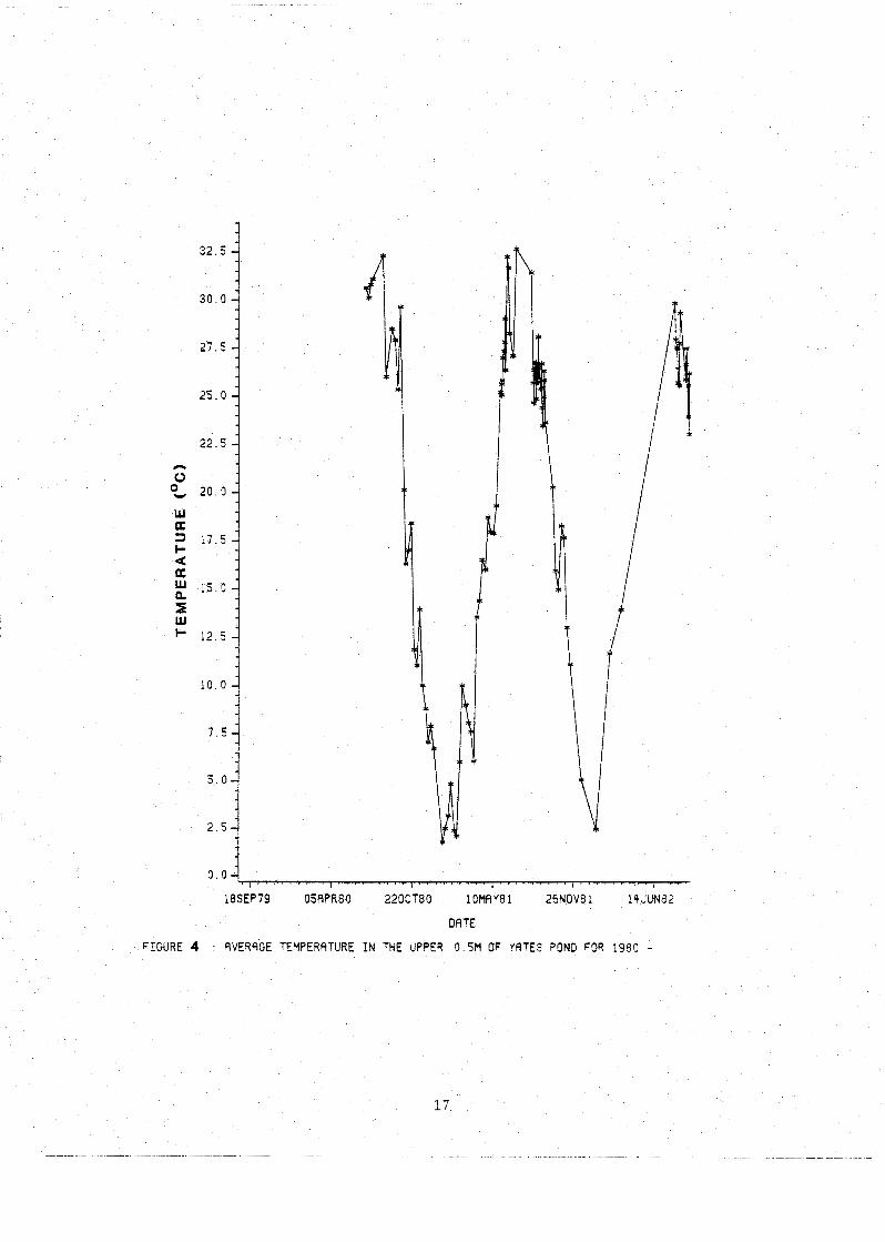
mid-August. During the summers of 1980 and 1981 the average

temperature of the upper 0.5 m of the water column exceeded

31°c (Fig. 4) while the surface layer itself was hotter

than 33Oc. Minimum surface temperatures of 1-2O~ were

measured in January of both 1981 and 1982.

Effects of turbidity manipulations on temperature

The subponds, maintained at three different turbidity

levels, only exhibited differences in temperature under the

certain environmental conditions. In early September 1982

temperature differences of 2 to 4OC were maintained for

one or two days before the wind would completely mix the

water column (Fig. 5). On 9/7/82 all subponds and Yates

were well mixed: control and alum-treated subponds had a

temperature of 22.9 OC, turbid was 22.1°c and Yates was

23.5 for an average temperature of 22.8'~. By the next

day the turbid subpond had an 0.25 m epilimnion, a

temperature of 28.7 and a 3.5 degree difference between 0.25

m and 0.5 m. The control subpond also had 0.25 m epilimnion

but was 2. ~ O C cooler at 26.4OC. The alum-treated

subpond was still well mixed with an average temperature of

23. ~OC. By 9/9/82 temperature differences were even greater. The turbid subpond had a 29.2°~, 0.25 m thick

epilimnion and a 4.5'~ temperature differential between

0.25 m and 0.5 m. The control subpond had a 26.8Oc, 0.25

m thick epilimnion and a 1.2Oc differential between the

epilimnion and the hypolimnion. The alum-treated subpond

had developed a temperature gradient to 0.75 m with an

average temperature of 25'~. The differential between the

turbid and alum-treated enclosures then was 4.2'~. During

this time the turbid enclosure had an average extinction

coefficient 7.83/m, a 1% light level of 0.6 m and a

turbidity level of 28 NTU. The alum-treated enclosure on

0 0 1 " " ' ~ I ~ " ' " ' ~ . ~ l . . . . . . ~ . , . ~ I . . ~ . I . ( . . . . I I . . I

18SEp79 05APR80 220CT80 1 0 M Y 8 1 26NOV8 1 lYJUN82

DOTE

FIGURE 4 SVERRGE TEMPERATURE I N THE UPPER 0 5M OF YATES POND FOR 1980 -

1 7

FIG. 5 TEYPESRTURE 4S DEPTH THROUGH TIME FOR SEPTEYBER 1982 EflCh BOX WIDTH I S 9 TEMPERATURE SRNGE F30M 20 TO 32 DEGREES

LEGEND Y=fRTES T=TURBID. 4= RLUM TRESTMEYT. C=CONTROL SYMBOLS * = YORNING SAMPLING = RFTEQNOON SAMPLING

the other hand had an extinction coefficient of 3.l/m, a 1%

light level of 1.5 m and a turbidity level of 13.5 NTU.

During 1981 and August 1982 (Fig.61, however,

thermoclines were much deeper than in September 1982 and

these extremes in temperature were not observed. For

example, between 8/7/81 and 8/17/81 the turbid enclosure had

an average thermocline depth of 1.4 m, an average extinction

coefficient of 5.76/m and the 1% light level at 0.8 m but

there was no difference in temperature between the subponds.

Plants and oxygen

Plant biomass varied greatly both between and within

years. In August 1981 the density and 95% confidence

intervals of the submerged macrophyte, Chara, for all 3

subponds was 257 270 g dry weight m-2. In September

1981 alum was added to the turbid enclosure and turbidity was added to the alum enclosure. At the end of the

experiments, the enclosure with increased light penetration also had an increase in bottom coverage of the plants. The

enclosure that received increased turbidity showed no change

in plant coverage over the 21 day treatment period (Table

4 ) . In the summer of 1982, no Chara was observed. With

the higher water levels in 1982, the emergent plant

Polygonum and the floating leaved plant Nuphar were inundated. During 1981 because of the low water, the beds

of most of these plants were out of the water.

FIG.6 TEMPESSTURE LIS OEPTH THROUGY TIME FOR AUGUST 1982 ERCh BOX WIDTY I S A TEYPESATdRE ?ANGE FROY 20 TO 32 PEGREF'

LEGEYD Y=YRTES T=TURBID 9 1 ALUM TREATYEYT. C=CONTSOL SYMBOLS t = YORVIYG SSMPLING = AFTERNOON SSYPLING

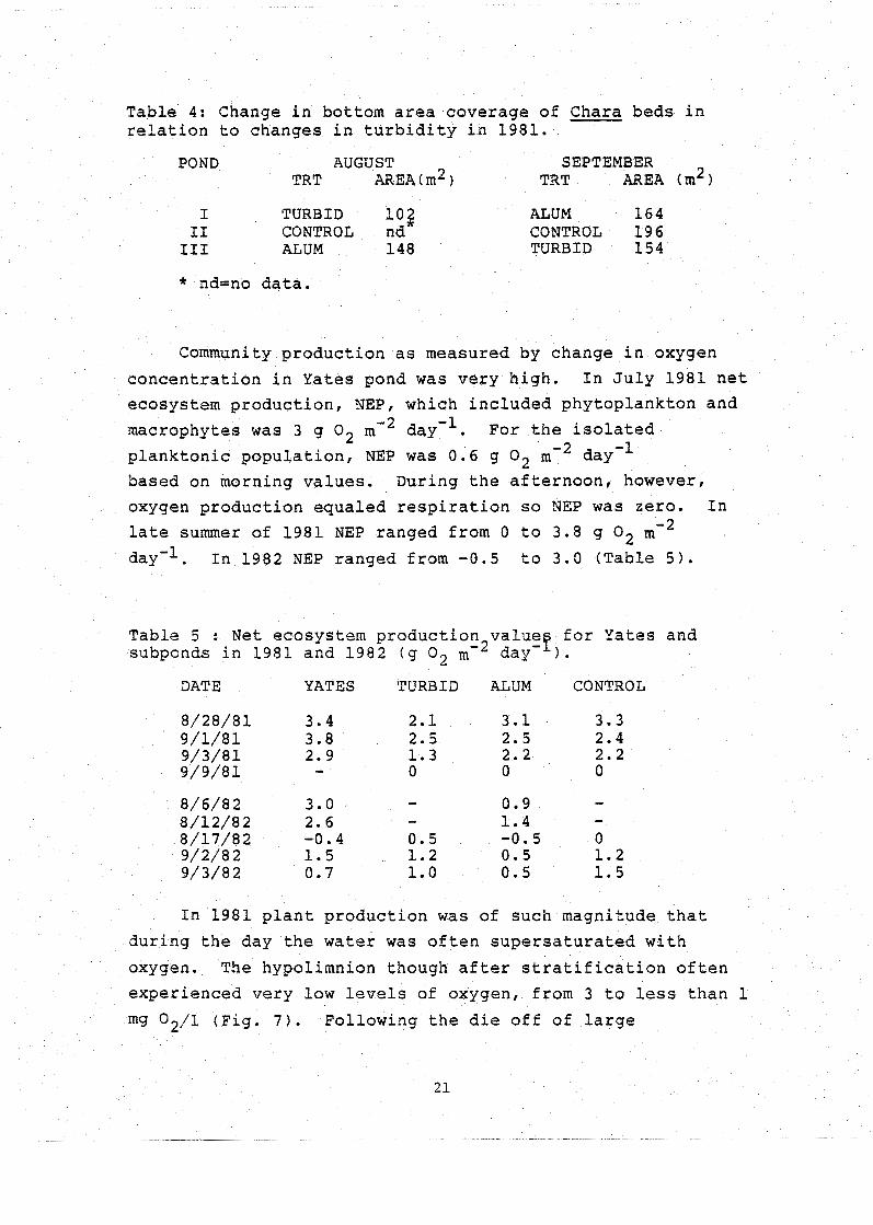
Table 4: Change in bottom area coverage of Chara beds in relation to changes in turbidity in 1981.

POND AUGUST SEPTEMBER TRT AREA(^^) TRT AREA (m2)

I TURBID 103 ALUM 164 I1 CONTROL nd CONTROL 196 I11 ALUM 148 TURBID 154

* nd=no data.

Community production as measured by change in oxygen

concentration in Yates pond was very high. In July 1981 net

ecosystem production, NEP, which included phytoplankton and -2 macrophytes was 3 g O2 m day-'. For the isolated

planktonic population, NEP was 0.6 g O2 m-2 day-'

based on morning values. During the afternoon, however,

oxygen production equaled respiration so NEP was zero. In

late summer of 1981 NEP ranged from 0 to 3.8 g O2 m-2

day-l. In 1982 NEP ranged from -0.5 to 3.0 (Table 5).

Table 5 : Net ecosystem production value for Yates and subponds in 1981 and 1982 (g O2 m-2 day-').

DATE YATES TURBID ALUM CONTROL

8/28/81 3.4 2.1 3.1 3.3 9/1/81 3.8 2.5 2.5 2.4 9/3/81 2.9 1.3 2.2 2.2 9/9/81 - 0 0 0

8/6/82 3.0 - 0.9 - 8/12/8 2 2.6 - 1.4 - 8/17/82 -0.4 0.5 -0.5 0 9/2/82 1.5 1.2 0.5 1.2 9/3/82 0.7 1.0 0.5 1.5

In 1981 plant production was of such magnitude that

during the day the water was often supersaturated with

oxygen. The hypolimnion though after stratification often

experienced very low levels of oxygen, from 3 to less than 1

mg 02/1 (Fig. 7). Following the die off of large

FIGURE 7 . DISSOLVED OXYGEN (MG/L) VS TIME - YATES POND AVERAGE CONCEYTRRTION FOR 0-0.5M (-+-I RND 1 .25-2 .0M ( -

blue-green algal blooms in both 1980 and 1981 the entire water column experienced low levels of oxygen, less than 3

mg/l, In 1982 oxygen concentrations in the epilimnion

during the summer were generally below saturation. In the

alum-treated subpond the entire water column was often near

Phytoplankton biomass as measured by chlorophyll a concentration fluctuated from summer lows of 5 ug/l to fall

peaks 100 and 300 ug/l for 1980 and 1981, respectively (Fig.

8). The peaks were due to blue-green algae. ~ccompaning

these periods of intense algal production were increases in

light extinction coefficient, Nt, decreases in secchi depth,

increases in chlorophyll a, CHL, suspended solids, TSS, and dissolved oxygen concentration, DO (Table 6).

Table 6 : Water quality parameters before, during and after a blue-green algal bloom in 1981. Measured during mid-day.

DATE CHL NTU TSS DO DO SECCHI Nt surf ace bottom

9/10 27 19 24 9.0 7.0 0.5 - 9/18 - 12 - 5.4 5.3 0.5 - 10/6 113 22 18 - - 0.5 3.7 10/13 197 28 - 14 14 0 .4 5.7 10/20 284 28 42 13 12 0.3 7.8 10/28 282 63 59 12 - 0.3 8.7 11/3 39 15 12 4 1.2 - 2.6 11/10 8 - - 3 2 1.0 - 2.4 11/18 25 - 9.4 9.1 1.1 1.9

Chlorophyll g : phaeo-pigment ratios were correlated to fall values for NTU, ~ ~ = 1 8 % n=49:

chl-a/phaeo = 10.2 - 0.17 NTU .

Regressions of this ratio against TSS and Nt, yearly as

well as seasonally, were not significant.

23

- - -- -- - - --

DRTE

FIGURE 8 W E W G E CYLOROPHYLL I N ThE UPPES 0 5 M OF f4TET

Mathematical model of the effects of turbidity and

backscattering on epilimnetic temperature change

In addition to absorbing light and converting that

energy into heat, particles may reflect light out of the water and into the air (backscatter) and thereby decrease

the total amount of radiant energy in the water. The

discussion that follows demonstrates that under certain

environmental conditions, temperature will increase as

turbidity increases until at high levels of turbidity

backscattering becomes significant and there is no further

increase in temperature.

The change in temperature is directly proportional to

the amount of radiation absorbed within the mixed layer and

inversely proportional to the depth of the mixed layer:

CTEMP = xIol / z ( 2

where: CTEMP is the change in temperature,

10' is the effective incoming radiation,

x is the percent of the light absorbed in the

mixed layer,

z is the depth of the mixed layer. It is assumed that each 1 cal/cc increase in

radiation will raise the temperature 1°c.

using equation 1, we can solve for depth, z, by knowing

that if x is the proportion of light absorbed in the upper layer then the depth at which (1-x) of the light remains

will be bottom of the mixed layer:

F u r t h e r , I o t , t h e e f f e c t i v e r a d i a t i o n r e m a i n i n g a f t e r

b a c k s c a t t e r i n g , c a n b e d e f i n e d a s :

10' = 10 (1 - B a c k s c a t t e r ) , ( 4 )

where : 10 i s t h e amount o f i n c o m i n g r a d i a t i o n a n d

B a c k s c a t t e r = 0.05 +0.00036TSS ( S t e f a n e t a l . 1 9 8 2 ) ( 5 )

From T a b l e 2 w e know TSS= 2 .7 + 1.1NTU

From T a b l e 3 , u s i n g t h e d a t a f o r a l l s e a s o n s ,

N t = 1 . 4 + 0.06NTU . ( 7 )

W e c a n t h e n a n s w e r t h e q u e s t i o n : "How d o e s t h e c h a n g e

i n t e m p e r a t u r e i n t h e mixed l a y e r v a r y a s a f u n c t i o n o f

t u r b i d i t y ? ' by s u b s t i t u t i n g e q u a t i o n s ( 3 ) t h r o u g h ( 7 ) i n t o

e q u a t i o n (2) :

CTEMP = - x I o ( 0 . 9 5 - 0.0004NTU) ( 1 . 4 + 0 . 0 6 N T U ) / l n ( l - X I .

w e c a n see t h a t c h a n g e i n t e m p e r a t u r e w i l l i n c r e a s e

u n t i l v e r y h i g h l e v e l s o f t u r b i d i t y a re r e a c h e d . W e c a n

a l s o see t h a t a t 25 NTU, b a c k s c a t t e r w i l l d e c r e a s e t h e

t e m p e r a t u r e c h a n g e b y a b o u t 1%, b u t t h e i n c r e a s e d

t e m p e r a t u r e c h a n g e d u e t o e n h a n c e d a b s o r p t i o n w i l l b e n e a r l y

d o u b l e d compared t o 0 NTU. T h i s r e q u i r e s t h o u g h t h a t t h e

mixed l a y e r d e c r e a s e a s t u r b i d i t y i n c r e a s e s .

I f t h e m i x i n g d e p t h i s g r e a t e r t h a n t h e e f f e c t i v e l i g h t

p e n e t r a t i o n d e p t h , t h e n t h e c h a n g e i n t e m p e r a t u r e i s no

l o n g e r d e p e n d a n t o n t h e (1-x) l i g h t d e p t h . The t e m p e r a t u r e

is a function only of the incoming radiation minus the

amount backscattered divided by the mixing depth. Therefore

turbidity does not increase the rate of temperature change when the mixed depth is greater than the effective light

penetration depth.

From these equations we can estimate the magnitude of

the effect that turbidity has on temperature. Assume that

backscattering is insignificant, as justified above; Nt -1.4

+0.06NTU ; mixing depth = 1% light level and Io=500 cal

cm-2 day-':

We conclude that for an increase in turbidity of 30 NTU

we can expect approximately a ~ O C increase in temperature

in the epilimnion on a bright summer day.

DISCUSSION

Turbidity was caused by inorganic particles in the

winter and by blue-green algae during late summer and fall.

During winter, turbidity was controlled by storms. The

sheet flow of rain water washes soil off unvegetated land

and into creeks where along with resuspended bottom sediment

it is carried into the pond. The amount of time these

particles stay suspended is a function of the density and

size of the particle, density of the water and strength of

wind-generated water currents.

In the fall blue-green algal blooms were responsible

for increases in turbidity and for many changes in habitat

values. In October of 1980 a surface turbidity reading of

162 NTU was obtained which was twice as high as any other

observed reading for that year. Total suspended solids were

as high as 59 mg/l and the extinction coefficient peaked at

8.6/m. During the growth phase oxygen concentrations were

generally high during the day, but after they died, decomposition of the algae resulted in low oxygen

conditions. In 1981 the concentration of oxygen was 3-4

mg/l at the surface and less than 1 mg/l near the bottom.

Oxygen levels this low have been shown to be stressful to

fish (Doudoroff and Shumway 1970).

Summer turbidities were low, 10-20 NTU, due to

decreased runoff, decreased input of suspended solids and

the settling out of suspended particle in the epilimnion.

Turbidity was seasonally correlated with total

suspended solids. But the correlations were low due to the

variability associated with dissolved solids. A much higher correlation was obtained between the change in NTU

associated only with particles, i. e. before and after

filtration, and TSS. We found a 6 NTU increase in turbidity

for each 10 mg/l increase in TSS.

Light penetration was directly influenced by turbidity.

Each unit increase in NTU produced a 0.06 unit increase in

the extinction coefficient. A 1 mg/l increase in suspended

solids produced a 0.07 unit increase in Nt during the fall.

The intercept was 2.1. This is similar to the relationship

found by Stefan et al. (1982) for Lake Chicot in Arkansas:

Nt=1.9 + 0.045 TSS. Stefan et al. (1982) also analyzed

laboratory data reported by Witte et al. (1982) and found

Nt= 2.0 + 0.06 TSS. Stefan et al. Is equations though were

derived from secchi depth data where they assumed the secchi

depth represented the 15% light level. ~ccording to our

measures of secchi depths and direct underwater photometer

readings, secchi depth in the turbid enclosures and in the

pond itself represented the depth at which 30% of the

subsurface, 0 m, light remained. However, in the

alum-treated enclosures, the secchi depth was equivalent to

the 15% light level. This latter value is similar to

Vollenweider1s (1974) 15% light level and Wetzelts (1975)

range of 1-15%. The difference between the two turbidity

levels was due to the uniform absorption of wavelengths by

the suspended particles as in the turbid enclosures and the

selective absorption of wavelengths by the water and

dissolved material in the alum-treated enclosures. For

Yates pond, the average depth of the 1% light level,

considered to be the limit of the euphotic zone, ranged from

Light absorption by suspended particles was shown to

influence the temperature of the water. Water temperatures

affect organisms directly by influencing biochemical

reaction rates. Temperature also structures the environment

the organisms live in through the development of vertical

thermal gradients in the water column. The surface water is

generally well mixed by the wind, is generally well

oxygenated, and has a uniform temperatu're that is warmer

than the bottom. As summer progresses, the surface waters

heat up and the bottom waters become anoxic through

biological and chemical activity. These conditions compress

the space in which organisms can live. Fish, for example,

may be trapped in a zone between excessively high

temperatures at the surface with adequate oxygen and

adequate temperatures at the bottom but no oxygen.

As the number of particles in the water increases, the

depth to which the light is absorbed and converted into heat

decreases thereby concentrating heat in the upper layers.

We observed this phenomena in the subponds only in September

1982. During this period there was a ~ O C increase in the

epilimnion over the alum-treated enclosure. Analysis of the

model also showed that increased turbidity resulted in

increased temperature. Backscatter was important only at

high turbidity levels. A 25 NTU increase in turbidity

resulted in less than a 2% decrease in light energy due to

backscatter but the temperature increase per day increased

from 3.B0c/day at 10 NTU to 5.g0c/day at 35 NTU for

light = 2500 kcal mV2 d'l and a mixed depth of 0.25 m.

The final water temperature depends on environmental

conditions including air temperature, wind and evaporative

cooling. During September 1982, the stratification that

formed during the day was eliminated during the night and then reformed the next day. To put this in perspective, the

turbid enclosure had an NTU reading of 28 and extinction

coefficient of 7.8/m, the alum-treated enclosure values were

13 NTU and 3.l/m. This compares to turbidity levels for

Yates pond that range from 15 to 120 NTU. So Yates has the

potential to show temperature increases due to turbidity

fluctuations. The time when temperature increases may have a

detrimental effect, i.e. when the fish are close to their

upper lethal limit, occurs during the June, July and August

when the surface temperatures can be in excess of 30°c.

Our turbidity enrichment experiments in August of both

1981 and 1982 showed no temperature increase. During these

experiments, the depth of mixed layer was 0.75 m to 1.4 m

which was greater than the effective heating depth. As

discussed in the theoretical section on turbidity and

temperature, no increase in temperature would be detected if

the mixed layer was greater than the effective light

penetration level, the 1% light level, due to the

redistribution of heat. In fact the temperature may

decrease as cooler bottom waters are mixed with surface

waters. On the other hand as the depth of the mixed layer

approaches zero, the temperature increases and approaches

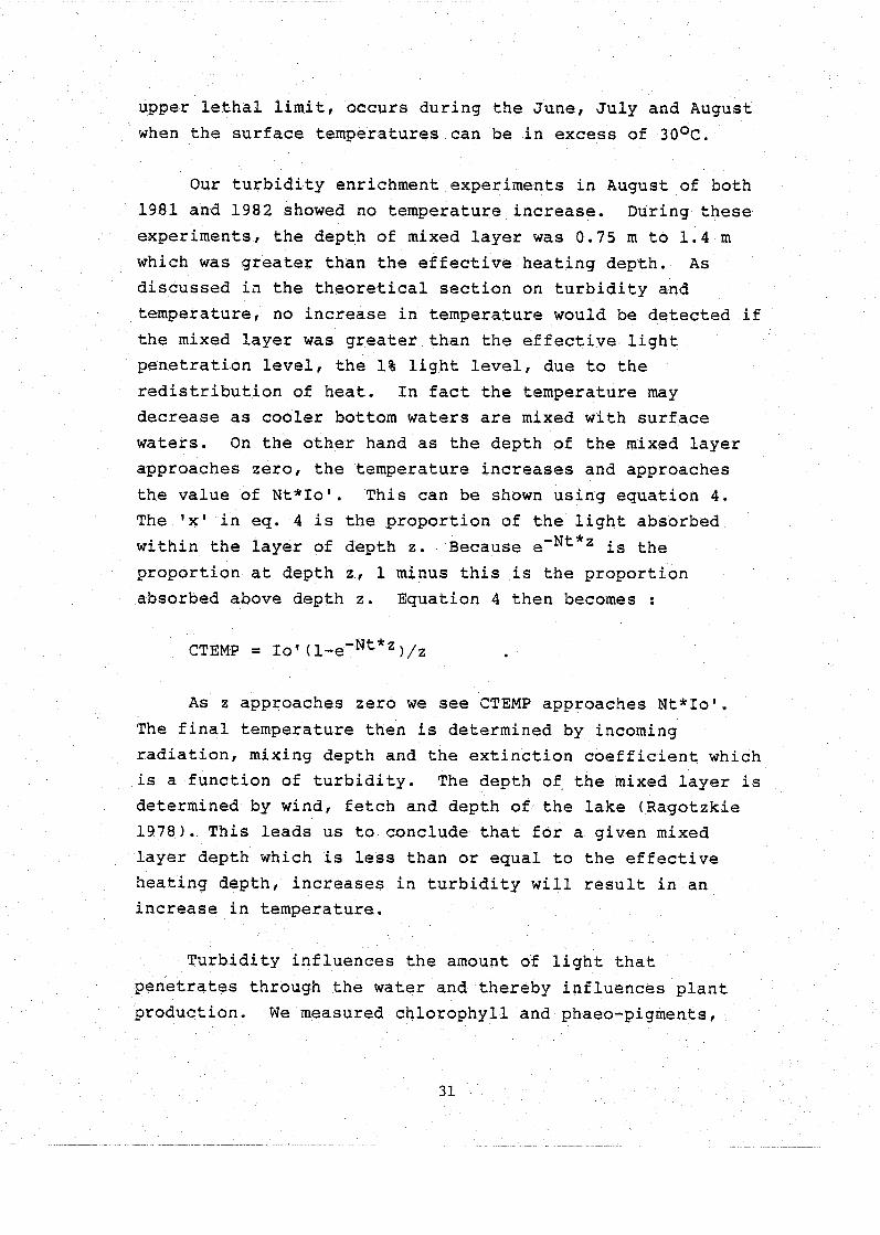
the value of Nt*Iog. This can be shown using equation 4.

The !xg in eq. 4 is the proportion of the light absorbed

within the layer of depth z. Because e is the

proportion at depth z, 1 minus this is the proportion

absorbed above depth z. Equation 4 then becomes :

CTEMP = Iog(l-e -N~*Z),/~

As z approaches zero we see CTEMP approaches Nt*Iog.

The final temperature then is determined by incoming

radiation, mixing depth and the extinction coefficient which

is a function of turbidity. The depth of the mixed layer is

determined by wind, fetch and depth of the lake (Ragotzkie

1978). This leads us to conclude that for a given mixed

layer depth which is less than or equal to the effective

heating depth, increases in turbidity will result in an

increase in temperature.

Turbidity influences the amount of light that

penetrates through the water and thereby influences plant

production. We measured chlorophyll and phaeo-pigments,

31

degraded chlorophyll, in order to determine the effect of

turbidity on algae suspended in the water column. One would

expect that as turbidity increased, algal production would

decrease and therefore the quantity of chlorophyll would

decrease. Algae though have the capability to increase the

total amount of chlorophyll per cell as the amount of light

decreases. Under conditions of prolonged low light levels,

the algae should die off and there should be a decrease in

the ratio of chlorophyll to phaeopigments. We found this

only in the fall.

Submerged macrophytes also appeared to be influenced by

light levels. Environmental conditions were not as

conducive to Chara growth in 1982 as they were in 1981.

In 1981 water level in the pond was nearly 0.75m lower than

pool stage, the turbidities averaged 16 NTU and the

extinction coefficient averaged 2.0/m. These conditions

enabled light to reach the bottom, the 1% light level was

2.7 m, and promoted extensive development of Chara and a

filamentous green algae. This in contrast to the summer of

1982 where extinction coefficient averaged 4.5/m, the 1%

light level was at 1 m and the water level was near normal

pool stage. As a result, sufficient light could not reach

the bottom and submerged macrophytes were not observed.

Under extremely high turbidity levels, submerged

plants may be killed. If the turbidity levels do not kill

the plants, they may be sufficiently high to cause the

plants in deep water to die back to a point where the light is adequate. In 1981 Chara was growing in the

alum-treated subpond in August. In September suspended matter was added to the alum subpond. At the end of the

treatments (21 days) no significant change in the horizontal

extent of the plant bed was found. But we did find a 60%

increase in areal coverage when then turbidity was reduced.

The macrophytic production in Yates pond was of such

magnitude that during 1981 the water was often

supersaturated with oxygen. In July 1981 we found that planktonic production equaled respiration and was

insignificant relative to the macrophytic release of oxygen.

During August 1982 production was lower than August 1981

and the waters were often undersaturated. The main

difference between these two years was the development of

submerged plants. It appeared that increased turbidity may

have restricted the development of Chara. The luxuriuos

stands we found in 1981 were not present in 1982. There

were other aquatic plants in the pond but their gas exchange

surfaces are usually out of the water, e. g. Nuphar and

Polygonum.

A.P.H.A.

and

Baumann,

LITERATURE CITED

1975. Standard methods for the examination of water

wastewater. Am. Public Health Assoc., Inc. 769 pp.

P.C. and J.F. Kitchell. 1974. Die1 patterns of

distribution and feeding of bluegill in Lake Wingra,

Wisc. Trans. Am. Fish. Soc. 103(2):255-260.

Bietinger,T.L. and J.J. Magnusson. 1974. Growth rates and

temperature selection of Bluegill, Lepomis

macrochirus. Trans. Am. Fish. Soc. 108:378-382.

Buck, D.H. 1956. Effects of turbidity on fish and fishing.

Trans. North Am. Wildl. Conf. 21:249-261.

Byrd, I. B. 1951. Depth distribution of bluegill, Lepomis

macrochirus Rafinesque, in farm ponds during summer

stratification. Trans. Am. Fish. Soc. 81:162-170.

Coutant, C. C. and D. K. Cox. 1976. Growth rates of subadult

largemouth bass at 24 to 35.50C. In: Thermal Ecology - 11. G. W, Esch and R. W. McFarlane, Eds. Tech. Inform.

Center, ERDA. p. 118-120.

Coutant, C. C., H. M. Ducharme, Jr., and J. R. Fisher. 1974.

Effects of cold shock on vulnerability of juvenile

channel catfish (Ichtalurus punctatus) and

largemouth bass (Micropterus

predation. J. Fish. Res. Bd.

salmoides to

Can. 31:351-354.

Doudoroff, P., 1969. Developing thermal requirements for

freshwater fishes. In: Krenkel, P.A., and F.L. Parker, Eds. Biological aspects of thermal pollution.

Vanderbilt U. Press. 407 p.

Doudoroff, P. and D.L. Shumway. 1970. Dissolved oxygen

requirements of freshwater fishes. FA0 Fisheries

Technical Paper No. 86:291p.

Dunst, R.C. 1969. Cox Hollow Lake: The first eight years of

impoundment. Wisc. Dept. Nat. Resources Res. Rep. 47.

19 p.

Eggers, D.M. 1977. The nature of prey selection by

planktivorous fish. Ecology 58:46-59.

Ellis, M.M. 1944. Water purity standards for freshwater

fishes. Bur. Fish, Spl. Sci. Rept. No. 2. 16 p.

Frey, D.G. 1955. Distributional ecology of the cisco

Coregonus artedii in Indiana. Invest. Ind. Lakes

and Streams Vo1. IV: 177-228.

Gardner, M.B. 1981. Effects of turbidity on feeding rates

and selectivity of bluegills. Trans. Am Fish. Soc.

Hall, D.J., W.E. Cooper, and E.E. Werner. 1970. An

experimental approach to the production dynamics and

structure of freshwater animal communities. Limnol.

Oceanogr. 15(6):839-928.

a Ei t i

w m 4 0 c

0 m u m c, c u c m a ) Q ) k w P I3 w 3 1 W X

0

m rl m

r,

C k

m 0 ** rl C C k -4 HI U C

Err U

a) O r :

5 m r l E w m 3 : C -4 -4 d .

m pr; w m P (\1 k k 5 l o o c o c, m .-I U 4 m r d s a Err l U a m **

-4 W 3 3

w - r l . P C ( F a % w m C 4 - 4 . -

C3 k 'tl a,

0 . . tJ c

X m H a ,

$ E H U c h

. a m ; C k O k o a r l o m 4 0 w C O U C - 4 4 J W H I: U I)

m rl rl

rl (V

I cll a3

cn rl

U ** d' . PI

m 4J c a

a o x u El

Lorenzen, C.J. 1966. A method for the continuous measurement

of & vivo chlorophyll concentration. Deep-sea Res. 13:223-227.

Magnusson, J.J., L.B. Crowder, and P.A. Medvick. 1979.

Temperature as an ecological resource. American 2001.

19:331-343.

Moss, D.D., and D.C. Scott. 1961. Dissolved oxygen

requirements of three species of fish. Trans. Am. Fish.

SOC. 90(4):377-393.

Neill, W. H. and J. J. Magnuson. 1974. Distributional

ecology and behavioral thermoregulation of fishes in

relation to heated effluent from a power plant at Lake Monona, Wisconsin. Trans. Am, Fish. Soc.

1034(4):663-710.

Peterson, S. T. and R. M. Schutsky. 1976. Some

relationships of upper thermal tolerances to preference

and avoidance responses of the bluegill. 2: Thermal Ecology 11. G. W. Esch and R. W. McFarlane, Eds. Tech.

Inform. Center ERDA p. 148-153.

Plumb, J.A. 1973. Effects of temperature on mortality of

fingerling channel catfish (Ichtalurus punctatus)

experimentally infected with channel catfish virus. J.

Fish. Res. Board Can. 30(4):568-570.

Radtke, L. D. and J. L. Turner. 1967. High concentrations

of total dissolved solids block spawning migration of striped bass, Roccus saxitalis, in the San Joaquin

River, California. Trans. Am. Fish. Soc.

Ragotzkie, R.A. 1978. Heat budgets of lakes. pp. 1-20

Lerman, A.,ed. Lakes: chemistry, geology, physics.

Springer-Verlag New York, Inc. New York. 361 pp.

Stefan, H.G., S. Dhamotharan, and F.R. Schiebe. 1982.

Temperature/sediment model for a shallow lake. J.

Environ. Eng. Div. 108(EE4):750-765.

Strawn, K. 1961. Factors influencing the zonation of

submerged monocotyledons at Cedar Key, Florida. J.

Wildl. Manag. 25(2):178-189.

Swallow, W. H. 1968. The relation of incubation

temperature to the mortality of fish embryos. M. S.

Thesis, Cornell Univ., Ithaca, N. Y. 45 p.

Swenson, W. A. and M. L. Matson. 1976. Influence of

turbidity on survival, growth, and distribution of

larval lake herring (Coregonus artedii). Trans. Am. Fish. Soc. 105(4):541-545.

Sylvester, J. R. 1972. Effects of thermal stress on

predator avoidance in sockeye salmon. J. Fish. Res.

Bd. Can. 29:601-603.

Vollenweider, R.A., ed. 1969. A manual of methods for

measuring primary production in aquatic environments.

Int. Biol. Program Handbook 12. Oxford Blackwell

Scientific Publications, 213 pp.

Vinyard, G. L. and W. J. OIBrien. 1976. Effects of light

and turbidity on the reactive distance of bluegill

(Lepomis macrochirus) J. Fish. Res. Bd. Can.

33(12):2845-2849.

Wallen, I. E. 1951. The direct effect of turbidity on

fishes. Bull. Okla. Agric. Mech. Coll. 48(1):1-27.

Webb, P.W. 1978. Partitioning of energy into metabolism and

growth. pp 184-214, In: S.D. Gerking. editor. Ecology of freshwater fish production. John Wiley and Sonsr New

York, NY, USA.

Weiss, C.M., and E.J. Kuenzler, 1976. The trophic status of

North Carolina lakes. Water Resources Research

Institute, University of North Carolina Report 119.

Raleigh, NC, USA.

Werner, E.E. 1979. Niche partitioning by food size in fish

communities. pp. 311-322 a: R.H. Stroud and H.

Clepper, eds. Predator-prey systems in fisheries

management. Sport Fishing Institute, Washington, DC.

Werner, E.E. and D.J. Hall, 1974. Optimal foraging and the

size selection of prey by bluegill sunfish (Lepomis

macrochirus). Ecology 55(5):1042-1052.

Wetzel, R.G. 1975. Lirnnology. W.B. Saunders Co.,

Philadelphia. 743 pp.

3 9

Whitmore, C. M., C. E. Warren and P. Doudoroff. 1960.

Avoidance reactions of salmonid and centrarchid fishes

to low oxygen concentrations. Trans. Am. Fish. Soc.

Williams, L. G. 1966. Dominant planktonic rotifers of

major waterways of the United States. Limnol.

Oceanogr. 11(1):83-91.

Witte, W.G., C.H. Whitlock, T.W. Usry, W.D. Morris, and E.A.

Gurganus. 1982. Laboratory measurements of physical,

chemical and optical characteristics of Lake Chicot

sediment waters. NASA Technical Paper 1941. National

Aeronautics and Space Agency, Langley Research Center.

Vinyard, G.L. and W.J. O'Brien. 1976. Effects of turbidity

and light on the reactive distance of bluegill sunfish

(Lepomis macrochirus). 3. Fish. Res. Board Can.

33: 2845-2849.