the effects of the interstate commerce act on...

Rev Ind Organ (2013) 43:41–62DOI 10.1007/s11151-013-9394-8

The Effects of the Interstate Commerce Acton Transport Costs: Evidence from Wheat Prices

Bruce A. Blonigen · Anca Cristea

Published online: 16 July 2013© Springer Science+Business Media New York 2013

Abstract There is significant debate over the effect of the Interstate Commerce Act(ICA) on the cost of rail transport to shippers. Taking price differences across loca-tions as proxy for transport costs, we use data on wheat prices before and after theimplementation of the ICA to see if the Act led to smaller differences in wheat pricesacross American cities relative to a control group of European cities. We find that theICA had no effect on US transport costs; however, it reduced their volatility substan-tially. This evidence supports the view that the ICA helped stabilize cartel prices aftera period of significant price wars.

Keywords Cartel · Price wars · Railroad · Regulation · Threshold regression

1 Introduction

The Interstate Commerce Act (ICA) was adopted in the United States over 125 yearsago to address pricing practices by the railroad industry that were perceived as yield-ing prices that were too high and also discriminatory across markets. As part of thelegislation, the Interstate Commerce Commission (ICC) was formed to monitor pricesand policies of the railroad industry. The main charge of the ICC was to ensure fair andjust prices that were publicly posted, and to prohibit (except in special circumstances)

B. A. Blonigen (B) · A. CristeaDepartment of Economics, 1285 University of Oregon,Eugene, OR 97403-1285, USAe-mail: [email protected]

B. A. BlonigenNational Bureau of Economic Research, Eugene,OR 97403-1285, USA

123

42 B. A. Blonigen, A. Cristea

price discrimination—particularly in cases where rates were higher for shorter routesthan for longer routes.

Given the explicit cartel activities by railroads prior to the legislation and the factthat so many short-haul routes faced service from only a single (monopoly) railroadprovider, the effect of such legislation on competition and prices in the industry mightbe expected to be quite substantial and non-controversial. In other words, the traditionalview was that the ICA should have led to generally lower freight rates and had pro-competitive effects on the market.

However, a number of important reasons have been given for why such effects arefar from certain. First, as hypothesized by Kolko (1965), state regulations on railroadswere abundant beginning in the mid 1800s and may have already imposed regulationsthat were as strenuous as the federal regulations that came into effect with the ICA.

Second, the ICA legislation was far from specific in the charge that it gave to theICC to regulate the industry. Thus, it is not clear that the ICA would lead to anytangible changes in industry behavior. Perhaps more intriguing is what Gilligan et al.(1990) terms the revisionist interpretation that the ICA provided stable cartel pricesafter an extended period of volatile price wars.1 Stabilization of the cartel would meangreater profits for the railroads at the expense of consumers. Relatedly, one of themore specific parts of the regulation was the requirement that railroads make theirrates public. While this created transparency, it could also have had the unintendedeffect of helping to support collusion amongst railroad firms.

Finally, Aitchison (1937), MacAvoy (1965) and others document how a string ofcourt rulings within the first decade of the Act led to potentially significant mitigationof the ICA’s scope and the ICC’s power to enforce the ICA.

Despite the theoretical ambiguity of ICA effects, there has been little analysis toassess quantitatively its economic effects due in large part to data availability issues.Spann and Erickson (1970) use industry level data on railroad costs and quantities, ratechanges across short- and long-haul routes, and assumptions on demand to estimatethe consumer surplus effects of the ICA. Key to their analysis is evidence from a surveyof rates that indicate the extent to which long-haul rates increased and short-haul ratesfell due to the non-discrimination statutes of the ICA. They estimate that the losses toconsumers from rate increases on the long-haul routes were twice as large as the gainson the short routes from lower rates. In a follow-up study, however, Zerbe (1980) showsa number of errors in the Spann and Erickson (1970) calculations that lead to a quiteopposite conclusion: Gains in the short-haul routes outweigh the losses in the long-haulroutes. A related concern for both studies is that they use “a small sample of 1886 and1890 prices for various distances” as their key data (Spann and Erickson 1970, p. 239).

Another set of papers has used event study analysis to examine the impact of ICA-related events on the stock prices of railroads during the period. According to the well-known capital-asset pricing model (CAPM), changes in a firm’s stock price shoulddirectly reflect changes in a firm’s expected future discounted profits. Binder (1985)studies over 20 different US regulatory events, and finds no statistically significant

1 See Porter (1983) for an interesting theoretical and empirical analysis that confirms switches in industrybehavior from cartel pricing to non-cooperative oligopoly pricing in the years immediately preceding theICA.

123

ICA and Wheat Prices 43

abnormal returns to the related firms’ stock price returns when most of these regulatoryacts were publicly announced, including in the case of the ICA. This leaves open thequestion of whether the regulatory events had no effect on firms’ profits or whetherthe event study approach is not adequate for identifying such effects.

Prager (1989) focuses explicitly on the events surrounding the ICA and subsequentcourt rulings in the 1890s that may have significantly affected the interpretation ofthe ICA or the abilities of the ICC to enforce it. Her analysis finds some evidence ofa modest positive abnormal return for the railroads from the passage of the ICA, butstronger evidence that subsequent court rulings that limited the powers of the ICC hadsignificant negative effects on railroad’s profitability. This provides evidence in favorof the revisionist view that the ICA was (initially) more beneficial to the railroads thanthe farmers and other users of rail transport.

Gilligan et al. (1990) also conduct an event study analysis of railroad firms’ returnsfrom ICA events and finds widely heterogeneous responses across both railroads andshippers (i.e., users of rail transport) to the introduction of the ICA, depending on suchfactors as whether they were mainly associated with short- or long-haul routes, andwhether they mainly served agricultural regions. They find some modest evidence thatshippers on short-haul routes and railroads on long-haul routes benefitted from thepassage of ICA. But like Prager (1989) they also find that these effects were largelyreversed by subsequent court decisions.

Beyond Spann and Erickson (1970) small survey of post-ICA changes in rail rates,a few other studies have collected data on railroad transport rates from this time period,but don’t really focus on evaluating the effects of the ICA. MacAvoy (1965) looks atmovements in shipments, rail rates, and price differences between Chicago and NewYork for wheat and lard, both before and after the ICA. However, he does not use thedata to look for any systematic change due to the ICA. Binder (1985) uses similar datato examine the impact of a 1897 court ruling that the railroad industry violated the1890 Sherman Antitrust Act (not the ICA) on rail industry performance, and finds noeffect of the ruling on rates charged to transport lard between Chicago and New York.

A real issue for these studies is data availability, as they only rely on available ratesfor a few commodities for one route (Chicago to New York). Also, they use postedrates; but there is the real concern that railroads provided special deals to enoughcustomers even after the ICA that the effective rates could be quite different fromposted rates (MacAvoy 1965). As a way around the difficulty of finding available andappropriate data on transport costs, recent literature has refined techniques to infer (orestimate) transport costs across locations using more available data on differences inmarket prices of commodities at each location. Such studies include O’Rourke et al.(1996), Ejrnaes and Persson (2000), Persson (2004), Jacks (2005, 2006), Shiue andKeller (2007), and Donaldson (forthcoming).

In this paper, we use a rich dataset on estimated transport costs for wheat constructedby Jacks (2005, 2006) for a large set of US and European cities in the 1800s and early1900s to evaluate the effect of the ICA. Grains have been a major commodity class forrailroads throughout history, with wheat comprising a large share of grain transport.Jacks estimates implied transport costs using wheat price differences for over 10,000city pairs from 1805 to 1910. While an ideal data set would have such observations forfreight rates, rather than estimated transport/arbitrage costs, Jacks database is the best

123


that is available. We employ a difference-in-differences strategy to examine whetherUS cities saw significant changes to these transport costs in the wake of the ICA in1887. The many European city pairs in the data provide a useful control group to allowus to identify the ICA effects on transport costs from common technological, demand,and supply shocks.

Our analysis uncovers a number of new and interesting results: First, there is nostatistical evidence that US wheat transport costs experienced any systematic changefrom the introduction of the ICA relative to world trends. This contrasts with thetraditional view that railroad rates would fall substantially in the wake of the ICA,but is consistent with revisionists’ arguments that the ICC interpretation of the ICAand initial court rulings strongly mitigated any need for the railroads to adjust theirrate structures. In contrast, we find that volatility in transport cost changes appears todecline significantly with the introduction of the ICA. This contrasts with the yearsimmediately prior to the ICA, which were characterized by sharp declines in transportcosts relative to trends. This evidence is consistent with the revisionist view that theICA helped stabilize cartel prices after a period of significant price wars.

2 The Debate on the ICA and Its Causes and Consequences

There are two types of views that are typically offered for why the ICA was ultimatelyintroduced in the US Congress and passed into law. The traditional view is that hightransport rates by railroads, particularly monopoly prices charged by railroads onshorter routes in agricultural regions, were the primary motive for the ICA. Andthis view makes much sense. The well-known Granger Movement was a coalition offarmers in agricultural regions of the United States that organized in the 1860s and1870s expressly to combat what were seen as monopoly prices by railroads to shiptheir products. They were able to push many states to adopt significant regulation onrailroads prior to the passage of the ICA (see Buck 1921; Miller 1971). Relatedly,Benson (1955) argues that merchants on the eastern seaboard of the US were anothergroup of downstream consumers of railroad transport that were also upset at high ratesand that were an important lobbying group for the ICA.

Examination of many of the main sections of the ICA regulation supports the tradi-tional view as well. After an initial section defines terms, Sects. 2, 3, and 4 specificallyaddress prices and make “unjust discrimination” illegal. Section 4 explicitly makes itillegal for a railroad to charge

greater compensation in the aggregate for the transportation of passengers or oflike kind of property, under substantially similar circumstances and conditions,for a shorter than for a longer distance over the same line, in the same direction,the shorter being included within the longer distance …

Section 5 makes pooling of freight rates illegal, and Sect. 6 establishes the ICC toenforce the ICA, with broad powers to “inquire into the management of the businessof all common carriers subject to the provisions of this act.” Thus, taken at face value,the ICA seemed quite intent to make certain that railroads charged “just” and “non-discriminatory” prices, with an oversight body given substantial powers to enforce

123


this mandate.2 And this would presumably remedy the key complaints by farmers andmerchants, and lead to lower rates, particularly on those routes that had little or nocompetition.

Kolko (1965) and MacAvoy (1965) are typically credited with introducing a revi-sionist view of the ICA, which has been supported by writings and analysis of subse-quent studies, including Spann and Erickson (1970) and Ulen (1980). The revisionistview begins by noting that the railroads had not been able to sustain cartels in thedecades prior to the ICA, with clear evidence of major oscillations from periods ofcartel pricing to substantial price wars. (see, e.g., Porter 1983). From this point therevisionist view splits a bit. Kolko (1965, p. 52) argues that because of their inabilityto maintain their cartels, railroads were big supporters of the ICA because the newly-formed ICC could coordinate cartel prices, concluding that “using the new law asauthority the railroads revamped their freight classification, raised rates, eliminatedpasses and fare reductions, and revised less-than-carload rates on all types of goods,including groceries.”3,4 In contrast, Ulen (1980) suggests that the railroads had devel-oped much more stable methods of maintaining their cartels (at least in normal marketperiods) in the early 1880s, and the ICA was basically ineffectual and did not preventthe railroads from maintaining their cartels. In this view, the railroads were not bigsupporters of passing the ICA, but were also not very concerned about its passage.

Regardless of one’s view about the intent of the ICA, it is clear that a number ofsubsequent events likely weakened its effects. First, MacAvoy (1965, p. 113) suggeststhat the ICC’s first report setting practical standards in implementing the ICA “left thestrong impression at once that rate discrimination, within prescribed limits, was legal.”In other words, interpretation of the law under the ICC would be broad, not strict, thusmitigating the potential policy impact of the ICA. Perhaps more important were anumber of subsequent court rulings in the following decade that questioned the ICC’srole in setting rates in the industry (the “Maximum Freight” case of 1897) and thatstruck down existing ICC standards and broadened interpretations of the ICA short-haul/long-haul sections (the “Osborne decision” of 1892, the “Social Circle case” of1893, and the “Troy case” of 1897). Echoing the sentiment of much of the literature,Aitchison (1937) concludes that by 1897 court decisions had rendered the existingICA “futile.”

3 Hypotheses

Given our data, we wish to examine how the ICA affected US transport costs, whererailroads were a significant portion of transport for the commodity that we examine:

2 See Aitchison (1937) for a detailed description of the ICA.3 He also notes a memo from an ICC Commissioner, Aldace F. Walker, who resigned after his first 2 years totake another position, indicating the Commissioner’s opinion that the ICC was more effective at maintainingcartel prices than the railroads’ own “pool” prior to the ICA.4 Relatedly, the “Wabash decision” in 1886 was a court ruling that prohibited states from regulating railroadson interstate transport, setting the stage for the passage of the ICA to establish federal regulation of interstatetransport. This is viewed by many as a substantial gain for railroad interests as well, because it eliminatedmany state regulations that had become quite severe in some circumstances.

123


wheat. However, from the discussion above, it is difficult to get a definitive hypothesisfrom the literature about what effects the ICA would have on railroad rates. This maybe especially true of long-haul rates, which we believe our analysis will primarilyidentify from using the major city-pairs in our data. Given this, our null hypothesis isthat the ICA did not have any statistically significant effect on the long-haul transportcosts that we examine.

The most obvious alternative hypothesis is that transport costs on long-haul routesrose after the ICA due to two reasons. First, the anti-discrimination provisions of theICA would put pressure on the railroads to raise more competitive long-haul rates,while decreasing rates on monopolized short-haul routes.5 Second, the transparentposting of prices and the involvement of the ICC to mediate rate wars could helpsupport more stable and higher cartel prices on the competitive long-haul routes. Asecond alternative hypothesis is that transport costs fall in our sample after the ICA.This would be the case if many of our routes were actually monopolized at the time(despite being fairly long-haul distances) and therefore saw pressure for them to fallin order to satisfy anti-discrimination requirements.

We can also examine the extent to which the ICA affected the volatility in transportcosts due to the ICA, which is a novel question for the literature on the effects ofthe ICA.6 In fact, an examination of this issue can help us assess which of the tworevisionist’s viewpoints is correct: Did the ICA help create a stable cartel for therailroads? Or was it largely ineffectual in altering market behavior? Our null hypothesisis that there is no effect of the ICA on the volatility of transport costs. This wouldbe supportive of the revisionist point of view that argues that the ICA was ineffectualand did not alter market behavior. The alternative hypothesis is that the ICA reducedvolatility due to the creation of a more stable cartel environment, as suggested byothers from the revisionist viewpoint. There do not appear to be any implicationsfor the effect of the ICA on transport cost volatility that stem from the traditionalviewpoint.

4 Data

Our aim is to evaluate the economic effects of ICA on the US rail transportation sector,by comparing them to the outcomes in a control group that is formed by markets thatwere not targeted by the policy change. For this effort, one needs consistent data ontransport costs across both US and non-US locations for a sufficient time period, bothbefore and after the implementation of the ICA. This is a seemingly impossible datatask for a period such a long time ago. However, there have been a number of recent

5 Spann and Erickson (1970) estimate from their limited survey that rates fell 15–30 % on short-haul routesand went up only slightly on long-haul routes. MacAvoy (1965) provides a more detailed, and complicated,picture about how rates changed. Posting of public rates subsequent to the passage of the ICA appears tohave led to the elimination of “special”, discriminatory rates for certain customers, tending to keep rateshigher. Yet, even within the first year, there were examples of competitive rate decreases on the longer haulroutes.6 Dennis (1999) is an example of the estimation of the impact of railroad deregulation on volatility oftransport costs in another (more modern) setting: steam coal rates after the 1980 deregulation.

123


efforts in the trade and economic history literatures to infer trade and transportationcost information from the commodity price margin between two locations (Shiueand Keller 2007; Jacks 2005, 2006; Ejrnaes and Persson 2000; Canjels et al. 2004;Goodwin and Grennes 1998).

For this project we use the dataset from Jacks (2005, 2006), which includes animpressive set of variables that characterize the wheat markets across cities in the USand Europe during the nineteenth century. The unbalanced sample covers a total of 102cities from 10 countries (see Appendix Table 5 for a complete list of country and citycoverage), which are observed at 5-years intervals over the period 1805–1910. Thethirteen US cities covered in our sample are Alexandria, Chicago, Cincinnati, Indi-anapolis, Ithaca, Kansas City, Minneapolis, New Orleans, New York City, Philadel-phia, Richmond, St. Louis, and San Francisco. Importantly, grain was the primaryproduct transported by rail during this period. Ripley (1906) reports that 73 % of allrail tonnage was grain as of 1882.7

A unit of observation in our dataset is a city pair. For each city-pair, we have infor-mation on geography (distance, waterways, border), current transportation technology(railroads, water), indicators of social and economic integration (common language,gold standard adherence, monetary union, ad valorem wheat tariffs, trade prohibition),and conflict variables (effects of war and war alliances). Critical for our analysis, thedataset from Jacks (2005, 2006) includes estimates of trade costs at the city-pair level,covering the entire sample period. In this paper, we will use the estimated trade costsas a proxy for the transportation cost between two locations. Even though Jack’s esti-mated trade costs may capture other trade frictions than transportation costs, the abilityto directly control for these alternative impediments to trade mitigates this problem.Table 1 reports the summary statistics for the variables in our sample.8 Given themethodology below, the transportation costs are measured as a percent (in decimalform) of the average wheat price across the two cities in the bilateral-city pair.

The methodology to uncover transportation costs between locations using only pricedata is founded on the simple idea of arbitrage. Whenever the wheat price differencebetween two locations becomes larger than the cost of transporting the good, arbitragewill occur so that the price difference is no larger than the transport cost. Followingthe notation of Jacks (2005, 2006), suppose transport costs in a given time period tfrom city 1 to city 2 are denoted as C12

t , and transport costs in the reverse direction intime period t are denoted as C21

t . Then the difference in the two prices in cities 1 and2, P1

t and P2t respectively, will satisfy the following conditions due to arbitrage:

− C12t ≤ (P1

t − P2t ) ≤ C21

t (1)

−C21t ≤ (P2

t − P1t ) ≤ C12

t (2)

7 We are unable to find data for only wheat shipments for this general period, even from Interstate CommerceCommission reports, but others (e.g., Fogel 1964) note that wheat and corn were the two main grainshipments at the time.8 See Table 2 in Jacks (2006) and related online data appendices at http://www.sfu.ca/~djacks/data/publications/publications.html for further details on data sources and measurement.

123

http://www.sfu.ca/~djacks/data/publications/publications.html



Table 1 Summary statistics

Variable Obs Mean SD Min Max

Transportation cost 11,578 0.384 0.267 0 1.954

Distance (thousands of miles) 11,578 2.531 3.232 0.030 27.270

Distance squared (millions of miles) 11,578 16.846 48.548 0.001 743.649

Exchange rate volatility 11,540 0.005 0.019 0 0.156

Border 11,578 0.466 0.499 0 1

Railroad 11,578 0.440 0.485 0 1

Railroad×distance 11,578 571 1,342 0 8,079

Canal 11,578 0.050 0.218 0 1

River 11,578 0.028 0.166 0 1

Port 11,578 0.099 0.299 0 1

Gold standard 11,578 0.111 0.302 0 1

Monetary union 11,578 0.021 0.142 0 1

Common language 11,578 0.065 0.247 0 1

Ad valorem (tariff) 11,578 0.070 0.158 0 0.983

Prohibition 11,578 0.073 0.197 0 1

Neutral 11,578 0.026 0.093 0 1

Allies 11,578 0.008 0.077 0 1

At war (external) 11,578 0.014 0.102 0 1

At war (internal) 11,578 0.051 0.167 0 1

Civil war (external) 11,578 0.021 0.086 0 0.621

Civil war (internal) 11,578 0.019 0.081 0 0.621

The sample covers the time period 1805–1910 in 5-years intervals. Transportation costs are measured as apercent (in decimal form) of the average wheat price across the two cities in the bilateral-city pair. See Table 2in Jacks (2006) and related online data appendices at http://www.sfu.ca/~djacks/data/publications/publications.html for further details on data sources and measurement

This setting allows Jacks to estimate transport costs and speed of arbitrage(or “adjustment”) through a regression technique called an asymmetric-thresholderror-correction-mechanism (ATECM) model.9 The intuition is that the change inprices for a given city each period follows a random walk (due to exogenous shocks inthe local environment) unless that city’s price differential with another city is greaterthan the transport costs between the two cities; that is, one of the conditions in Eqs.(1) or (2) is violated. When a condition is violated, there will be arbitrage of the pricesfrom period t − 1 to period t . The degree of arbitrage that can occur in one period iscaptured by an adjustment parameter, −1 ≤ ρ ≤ 0, where a value of −1 indicatescomplete arbitrage in just one period. Denoting, a city i’s change in prices from periodt − 1 to period t as �Pi

t , we can write down the following ATCEM model for theadjustment in prices over time for the city pair:

9 Further details on the econometrics of threshold regression techniques can be found in Balke and Fomby(1997), Hansen (1997), and Hansen and Seo (2002)

123




�P1t =

⎧⎪⎪⎪⎨

⎪⎪⎪⎩

ρ1

(P1

t−1 − P2t−1 − C21

t−1

)+ η1

t if P1t−1 − P2

t−1 > C21t−1

η1t if − C12

t−1 ≤(

P1t−1 − P2

t−1

)≤ C21

t−1

ρ1

(P1

t−1 − P2t−1 + C12

t−1

)+ η1

t if P1t−1 − P2

t−1 < −C12t−1

(3)

�P2t =

⎧⎪⎪⎪⎨

⎪⎪⎪⎩

ρ2

(P2

t−1 − P1t−1 − C12

t−1

)+ η2

t if P2t−1 − P1

t−1 > C12t−1

η2t if − C21

t−1 ≤(

P2t−1 − P1

t−1

)≤ C12

t−1

ρ2

(P2

t−1 − P1t−1 + C21

t−1

)+ η2

t if P2t−1 − P1

t−1 < −C21t−1

, (4)

where we assume (η1t , η

2t ) ∼ Nid(0,�). The system of equations can then be esti-

mated via seemingly unrelated regression (SUR), where the log-likelihood functionis

log L = −T M

2log(2π) − T

2log |�| − 1

2

T∑

t=1

η′t�

−1ηt , (5)

where T is the number of observations, and M is the number of equations.While it is straightforward to see how the adjustment speed parameters, ρ1 and ρ2,

are estimated in this model, the major complication is unavailable data on transportcosts—the key variables of interest to our study. Jacks (2005, 2006) is able to estimatethese transport costs within the estimation system by calculating the log-likelihoodfor all possible transport cost values for any given pair of city in a given time period,and choosing the combination of transport costs, C12

t−1and C21t−1, that maximize the

log-likelihood function for the observed set of prices. Through this computationallyintensive procedure, he can then provide estimates of C12

t−1 and C21t−1 and their standard

errors. It is these estimates that we can then use for our estimation of the effects of theICA on US transport costs.

5 Empirical Strategy

Our empirical strategy is to employ a difference-in-difference estimator to test whetherthe ICA reduced transport costs across US cities after it was introduced in 1887, vis-à-vis a control group of non-affected (i.e., non-US) cities.10

In line with Jacks (2006), we specify a model for the determinants of the bilateraltransport costs that characterize any two cities in our sample. Conditioning on othertrade frictions that inhibit arbitrage (i.e., wheat trade) and price convergence overspace, we evaluate the marginal contribution of the ICA to changes in transportation

10 A difference-in-differences specification simply estimates the relative effect of a “treatment” on a treatedgroup vis-à-vis a non-treated (or control) group with respect to a particular outcome (here, wheat transportcosts). This relative difference-in-difference effect is typically estimated by an interaction of a variable thatindicates a “treated” observation and a variable indicating the period of treatment. This is exactly how ourICAi j t variable is defined in Eq. (6), where the “treatment” is the ICA and our treatment group is the UScity-pairs in our sample. See Meyer (1995) and Angrist and Pischke (2008) for general discussion of themethodology.

123


costs. The baseline regression model that we take to the data is given by the followingequation:

T ransportCosti j t = β0 I C Ai jt + β1 Disti j + β2 Dist Sqi j + β3 Ex RateV oli j t

+β4 Borderi j + β5 Raili j t

+β6(Rail × Dist)i j t +β7Canali j t +β8 Riveri j +β9 Porti j

+β10Gold Sti j t + β11 MUi jt

+β12CommonLangi j + β13 AdV aloremi jt

+β14 Prohibi tioni j t +∑

k

ωkCon f lictki j t + ut + εi j t

(6)

where i, j and t index the origin city, destination city and year, respectively; andut denotes year fixed effects. The variable of interest is ICA, which is an indicatorvariable that takes the value of 1 for all US city pairs and all years following 1887,and zero otherwise. The coefficient β0 is identified from any systematic time variationin bilateral transport costs after 1887 across city-pairs within the US relative to theglobal transportation costs trend.

Many of the transport costs determinants included in the regression model are notonly standard in the trade literature, but also very intuitive. There is no doubt that bilat-eral distance (Disti j ) affects the cost of shipping wheat between two cities, and thesquared distance term (Dist Sqi j ) adds flexibility to the estimation, allowing for possi-ble non-linearities in the relation between distance and transport costs. Similarly, cross-ing a country border (Borderi j ) or sharing a common language (CommonLangi j ),both represent trade costs that directly influence the profitability of a cross-bordertransaction.

The exchange rate volatility (Ex RateV oli j t ) affects the cost of trading internation-ally by adding more risk to the transactions. Thus we expect β3 to be positive. Unlikethe unexpected exchange rate shocks, participation in a monetary union (MUi jt ) oradherence to the gold standard (Gold Sti j t ) provides a deeper level of economic inte-gration, which brings more certainty and stability in trade transactions. This impliesthat β10and β11 should be positive.

The transportation technology that is available between two cities at a point intime is another crucial determinant of the bilateral transport cost. The availability ofrailroads connecting two locations, their differential benefit for long- versus short-haultransport ((Rail × Dist)i j t ),the availability of canals (Canali j t ) and rivers (Riveri j )

connecting two cities, as well as the development of city ports (Porti j ), all contributetowards facilitating the movement of wheat between markets in search for arbitrageopportunities, thus contributing to an increased level of market integration.

The existence of ad valorem import tariffs for wheat ( AdV aloremi jt ) or, evenworse, prohibitions on wheat imports (Prohibi tioni j t ) directly affect the profitabilityof engaging in price arbitrage, and thus on the extent of price convergence and wheatmarket integration across cities.

Finally, given the turbulent periods of the nineteenth century, the regression modelaccounts for a vector of military-conflict-related variables (Con f lictki j t ) that Jacks

123


(2005, 2006) includes: We control for the fraction of time in a decade that the countriesof each city in the pair are in a war with each other (Atwar(external)i j t ), that thetwo countries are allied in war against a common enemy (Alliesi j t ), or one of thetwo trading partners is neutral when the other trading partner is at war (Neutrali j t ).We also control for the fraction of time that two trading partners (from the samecountry) see their country at war with another country (Atwar(internal)i j t ). In addi-tion, we include two war variables that are analogous to (Atwar(external)i j t ) and(Atwar(internal)i j t ), except for the case of a civil war rather than a war between twodifferent countries—(Civilwar(external)i j t ) and (Civilwar(internal)i j t ). Thewar-time measures are expected to have a negative effect on commercial relations,and thus increase transport costs, while being “neutral” or “allies” may have positiveeffects on commercial relations, as they mitigate the negative effects of war.

Since the dependent variable is an estimated variable, we estimate Eq. (6) using thegeneralized least squares (GLS) method, and rely on the number of observations usedfor generating the dependent variable as analytical weights.11 Furthermore, becausethe transport cost variable is generated for each sample year based on monthly pricedata that span 10-years overlapping periods, we also impose a first-order autoregressivecovariance structure.

While the model specification given by Eq. (6) controls for many transport costdeterminants, there may be other city-pair variables that are omitted from the regressionand possibly correlated with the ICA variable of interest. To account for this concern,we modify the baseline regression model by taking first differences. The resultingspecification can be written as follows:

� ln T ransportCosti j t = δ0�I C Ai jt + δ1�Ex RateV oli j t + δ2�Gold Sti j t

+δ3�MUi jt + δ4�Raili j t + δ5�Rail Disti j t

+δ6�Canali j t + δ7�AdV aloremi jt

+δ8�Prohibi tioni j t +∑

k

λk�Con f lictki j t +ut +εi j t

(7)

Note that by first differencing the regression model given by Eq. (6), the time-invariantcontrols drop out from the estimation. At the same time, first differencing the data alsomitigates concerns regarding the autocorrelation process that may be embedded byconstruction in our dependent variable. As before, we continue to use the numberof observations underlying the data-generating process for the dependent variable asanalytical weights, though necessarily taking the average over the two periods of thefirst difference.

The coefficient of interest is again δ0, and measures the effect of ICA on the transportcost of wheat between two cities, holding constant other determinants of transportcosts such as measures of economic integration (gold standard status, monetary union

11 Jacks reports that results are robust to weighting by other related measures, such as the standard erroror p value of the estimated transport costs. Saxonhouse (1976) provides the econometric theory for theapplication of such weights when using a generated dependent variable.

123


membership) or conflict/political instability. Note that by first differencing the ICAvariable, the non-zero observations used in identifying the coefficient of interest δ0corresponds to year 1890. Thus, the initial assumption that we are making is that theeffect of the ICA on transportation cost gets realized immediately (i.e., within a 5 yearstime interval), though we will later explore possible longer-run effects.

6 Empirical Results

6.1 Baseline Estimates

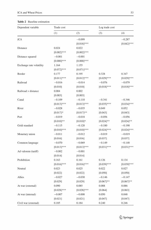
Table 2 reports the results from estimating the baseline regression model given by Eq.(6). For comparison purposes, column 1 reproduces the specification in Jacks (2006).Our estimates come very close to the ones that are reported in the original paper. Theyemphasize the main determinants of bilateral transport costs: distance and transporta-tion infrastructure (ports, canals), trade frictions such as exchange rate volatility, advalorem tariffs or trade prohibition, factors of economic integration such as gold stan-dard adherence, monetary union participation, and, finally, conflict variables such asinternal and external wars and civil wars.

In column 2 we add the ICA variable of interest, in addition to allowing for a separateintercept for US-only city pairs (i.e., Domestici j control variable). The negative andsignificant coefficient for ICA suggests that transport costs between two US cities fellon average by 0.10 relative to the control group of non-US cities. When evaluated atthe sample mean, this is equivalent to a fall in transport costs of 26 %.

In the next two columns of Table 1 we re-estimate the baseline model in Eq. (6)in log-log form.12 The benefits of expressing the continuous variables in log formare two-fold. First, it attenuates the significant skewness observed in the distributionof some of the key variables. Second, it removes any scale differences among theregression variables, and mitigates any distortionary effects of outlier observations.

Comparing column 3 to column 1, one can notice the consistency in sign andsignificance level across the two specifications. The same observations apply for theresults reported in column 4, relative to the corresponding estimates in column 2.Focusing on the variable of interest, we again find a negative and significant effect ofICA on the bilateral transport cost between US cities. The estimate suggests that, allelse equal, the rail regulation instituted by the ICA has led to a 24.9 % drop in transportcosts relative to the worldwide average trend. The magnitude of this effect is close tothe corresponding estimate from column 2, and it is consistent with the range of pricechanges documented in the existing literature (e.g., see Spann and Erickson 1970).

Nevertheless, as discussed in the previous section, one concern with the cur-rent model specification is that it does not control for city-pair fixed effects.This may be problematic because of the incidence of omitted variable bias.For example, regional specialization and the agricultural output of a locationare clear determinants of local wheat prices, directly influencing our estimated

12 The continuous variables that we express in log form are the transport cost, distance, distance squared,rail×distance, exchange rate volatility, and ad valorem tariff.

123


Table 2 Baseline estimation

Dependent variable Trade cost Log trade cost

(1) (2) (3) (4)

ICA −0.099 −0.287

[0.018]*** [0.042]***

Distance 0.024 0.022

[0.002]*** [0.002]***

Distance squared −0.001 −0.001

[0.000]*** [0.000]***

Exchange rate volatility 1.164 1.155

[0.072]*** [0.071]***

Border 0.177 0.195 0.328 0.347

[0.011]*** [0.012]*** [0.029]*** [0.029]***

Railroad −0.016 −0.014 −0.076 −0.079

[0.010] [0.010] [0.018]*** [0.018]***

Railroad×distance 0.004 0.002

[0.003] [0.003]

Canal −0.109 −0.110 −0.341 −0.346

[0.013]*** [0.013]*** [0.035]*** [0.034]***

River −0.028 −0.035 0.049 0.052

[0.017]* [0.017]** [0.043] [0.043]

Port −0.019 −0.018 −0.056 −0.056

[0.010]** [0.010]* [0.024]** [0.024]**

Gold standard −0.115 −0.120 −0.180 −0.190

[0.010]*** [0.010]*** [0.024]*** [0.024]***

Monetary union −0.011 −0.012 −0.019 −0.019

[0.016] [0.016] [0.037] [0.037]

Common language −0.070 −0.069 −0.149 −0.148

[0.013]*** [0.013]*** [0.031]*** [0.031]***

Ad valorem (tariff) −0.002 −0.001

[0.014] [0.014]

Prohibition 0.163 0.161 0.126 0.134

[0.016]*** [0.016]*** [0.039]*** [0.039]***

Neutral 0.023 0.025 0.022 0.027

[0.022] [0.022] [0.050] [0.050]

Allies −0.027 −0.030 −0.146 −0.147

[0.029] [0.029] [0.067]** [0.067]**

At war (external) 0.090 0.085 0.088 0.086

[0.028]*** [0.028]*** [0.064] [0.063]

At war (internal) −0.007 −0.008 0.050 0.048

[0.021] [0.021] [0.047] [0.047]

Civil war (external) 0.185 0.184 0.240 0.246

123


Table 2 continued

Dependent variable Trade cost Log trade cost

(1) (2) (3) (4)

[0.018]*** [0.018]*** [0.041]*** [0.041]***

Civil war (internal) 0.137 0.133 0.365 0.367

[0.021]*** [0.020]*** [0.047]*** [0.047]***

Domestic 0.146 0.196

[0.015]*** [0.038]***

Log distance 0.200 0.195

[0.010]*** [0.010]***

Log distance squared −0.042 −0.041

[0.005]*** [0.005]***

Log (1 + exchange rate volatility) 2.952 2.905

[0.171]*** [0.171]***

Railroad× log distance 0.042 0.044

[0.011]*** [0.011]***

Log (1 + ad valorem tariff) 0.118 0.117

[0.043]*** [0.043]***

Year fixed effects Yes Yes Yes Yes

Observations 11,539 11,539 11,537 11,537

The reported coefficients are obtained from text. The estimation method used is generalized least squares(GLS), with analytical weights given by the number of wheat price observations employed in the constructionof the transport cost dependent variable

transport cost measure. Similarly, geography, climate, and the existence and avail-ability of other modes of transport not directly controlled for in the model, rep-resent additional examples of factors that may influence the estimated transportcost.

6.2 First Difference Estimates

Without directly controlling for unobservable city-pair fixed effects in the model, anysystematic differences in transport costs that are specific to US cities are going to bepicked up by the ICA indicator. To avoid such omitted variable bias, in what followswe estimate the regression model in first differences, as described by Eq. (7).

Table 3 reports the results. Column 1 includes only the transport cost determinantsfrom the original Jacks (2006) paper, while column 2 adds our variable of interest,ICA. Unlike our initial estimates in Table 2, the effect of ICA on bilateral transportcosts is not distinguishable from zero after controlling for the city-pair fixed effects.13

13 Our first difference model imposes the constraint that the slope coefficients are common across US andnon-US city pairs. In unreported results, we have experimented with a more flexible model specificationthat also includes interaction terms between the regression variables and the indicator for US domesticcity-pairs. However, the ICA estimate remains insignificant.

123


Table 3 First difference estimation

Dependent variable � Log trade costs

(1) (2) (3) (4)

� ICA −0.006 −0.006 −0.021

[0.048] [0.048] [0.039]

ICA×year 1895 −0.016

[0.043]

ICA×year 1900 0.040

[0.061]

� ICA× ln distance −0.094

[0.053]*

� Exchange rate volatility 3.108 3.107 3.102 3.107

[0.191]*** [0.191]*** [0.191]*** [0.191]***

� Railroad −0.009 −0.009 −0.009 −0.009

[0.027] [0.027] [0.027] [0.027]

� Railroad× ln distance −0.026 −0.026 −0.026 −0.026

[0.013]** [0.013]** [0.013]** [0.013]**

� Canal 0.191 0.191 0.190 0.191

[0.069]*** [0.069]*** [0.069]*** [0.069]***

� Gold standard −0.140 −0.140 −0.139 −0.140

[0.037]*** [0.037]*** [0.037]*** [0.037]***

� Monetary union −0.013 −0.013 −0.013 −0.013

[0.036] [0.036] [0.036] [0.036]

� Log ad valorem 0.090 0.090 0.090 0.090

[0.051]* [0.051]* [0.051]* [0.051]*

� Prohibition 0.113 0.113 0.112 0.113

[0.044]** [0.044]** [0.044]** [0.044]**

� Neutral 0.018 0.018 0.018 0.018

[0.049] [0.049] [0.049] [0.049]

� Allies −0.201 −0.201 −0.200 −0.201

[0.073]*** [0.073]*** [0.073]*** [0.073]***

� At war (external) 0.055 0.055 0.056 0.055

[0.066] [0.066] [0.066] [0.066]

� At war (internal) 0.037 0.037 0.039 0.037

[0.044] [0.044] [0.044] [0.044]

� Civil war (external) 0.107 0.107 0.107 0.107

[0.047]** [0.047]** [0.047]** [0.047]**

� Civil war (internal) 0.088 0.088 0.088 0.088

[0.045]** [0.045]** [0.045]** [0.045]**

Year fixed effects Yes Yes Yes Yes

123


Table 3 continued

Dependent variable � Log trade costs

(1) (2) (3) (4)

R2 0.080 0.080 0.080 0.080

N 10,581 10,581 10,581 10,581

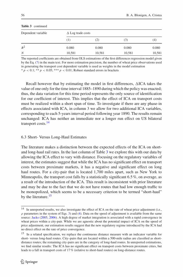
The reported coefficients are obtained from OLS estimations of the first differences regression model givenby the Eq. (7) in the main text. For more estimation precision, the number of wheat price observations usedin generating the transport cost dependent variable is used as weights in the model estimation* p < 0.1; ** p < 0.05; *** p < 0.01; Robust standard errors in brackets

Recall however that by estimating the model in first differences, �ICA takes thevalue of one only for the time interval 1885–1890 during which the policy was enacted;thus, the data variation for this time period represents the only source of identificationfor our coefficient of interest. This implies that the effect of ICA on transport costsmust be realized within a short span of time. To investigate if there are any phase-ineffects associated with ICA, in column 3 we allow for two additional ICA variables,corresponding to each 5-years interval period following year 1890. The results remainunchanged: ICA has neither an immediate nor a longer run effect on US bilateraltransport costs.14

6.3 Short- Versus Long-Haul Estimates

The literature makes a distinction between the expected effects of the ICA on short-and long-haul rail rates. In the last column of Table 3 we explore this with our data byallowing the ICA effect to vary with distance. Focusing on the regulatory variables ofinterest, the estimates suggest that while the ICA has no significant effect on transportcosts between proximate markets, it has a negative and significant effect on longhaul routes. For a city-pair that is located 1,700 miles apart, such as New York toMinneapolis, the transport cost falls by a statistically significant 6.5 %, on average, asa result of the introduction of the ICA. This result is inconsistent with prior literatureand may be due to the fact that we do not have routes that had low enough traffic tobe monopolized, which seems to be a necessary criterion to be termed “short-haul”by the literature.15

14 In unreported results, we also investigate the effect of ICA on the rate of wheat price adjustment (i.e.,ρ parameters in the system of Eqs. 3) and (4). Data on the speed of adjustment is available from the samesource: Jacks (2005, 2006). A high degree of market integration is associated with a rapid convergence inwheat prices within a city-pair. While we are agnostic about the potential impact of ICA on the speed ofprice adjustment, our estimation results suggest that the new regulatory regime introduced by the ICA hadno direct effect on the rate of price convergence.15 In a related specification, we replace the continuous distance measure with an indicator variable forshort- versus long-haul routes. City–pairs that are located within a 500-mile radius are classified as short-distance routes; the remaining city-pairs are in the category of long-haul routes. In unreported estimations,we find similar results: The ICA has no significant effect on transport costs between proximate cities, butleads to a fall in transport costs of 17 % (relative to short-haul routes) on long-distance routes.

123


Fig. 1 Transport cost changes after ICA by major city-pair. Notes (1) Each point in the scatterplot representsthe coefficient on the corresponding city-pair dummy variable that is obtained from estimating an augmentedversion of the regression model given by Eq. (7) in the main text. (2) Major cities are Alexandria (AL),Chicago (CH), Cincinnati (CI), Indianapolis (IN),Ithaca (IT), New York (NY), Philadelphia (PH), and SanFrancisco (SF)

To explore further the heterogeneity in ICA effects over distance, in unreportedmodel estimation, we allow the ICA coefficient to be city-pair specific (US citiesonly). Figure 1 plots the estimated slope coefficients against the city-pair bilateraldistance. Interestingly, the ICA coefficients involving San Francisco—the single WestCoast city in our sample—are systematically below the zero line. This sheds morelight on the underlying data variation that leads to the negative and significant effectof the ICA on long haul transport costs.16

6.4 Further Robustness Checks

To ensure the robustness of our findings regarding the effect of the ICA on the levelof transport costs, we perform several additional estimations. In the interests of space,we only describe the aim and outcome of these data exercises. These estimates areavailable upon request.

A possible concern with the current data sample and the resulting estimated coeffi-cients is the presence of US cross-border city pairs (i.e., international city pairs whereone city is in the US) as part of the model’s control group. These US internationalcity-pairs are composed of a US city that has seen some of its connections (its internalUS ones) “treated” by the ICA policy and a non-US city that has not seen any of its

16 We have also experimented with city-specific (rather than city-pair) ICA effects in order to see whetherthe insignificant effect of the ICA is due to opposing effects in monopolized versus competitive markets.The city-specific ICA coefficients turn out to be insignificant in most cases, except for a positive effect forIthaca and negative effect for San Francisco.

123


routes subject to this “treatment.” If the ICA effect on US shipments affects US cities’wheat shipment decisions to non-US cities, this interdependence could contaminatethe cross-ocean routes from the US, invalidating them as appropriate control groupobservations.

To investigate whether the insignificant effect of ICA on transportation costs isrelated to the inclusion of US international city-pairs in the control group, we re-estimate the model specification in first differences without these “ambiguous” city-pairs. The estimation results are very similar to the ones reported in Table 3, reinforcingthe conclusion of no significant impact of ICA on the level of bilateral transport costs.

The second robustness check that we perform investigates the sensitivity of ourresults to the elimination of all Chicago-based city pairs. The direct access of the cityof Chicago to the Great Lakes has made shipping via waterways an attractive andefficient transportation mode. In fact, as of 1870 over 90 % of wheat from Chicagotransported eastbound was going via the Great Lakes—not railroad. Because of thecompetition created by these alternative modes of transport, railway transportationprices involving the city of Chicago may look and respond differently to the ICA thanthe rest of the sample. Therefore, in unreported data exercises, we eliminate the city-pairs between Chicago and our east coast cities. Yet again, the main findings of thepaper continue to hold: The effect of ICA on transport costs remains insignificant.17

6.5 Examining the Impacts of the ICA on Transport Cost Volatility

As discussed in our hypothesis section, the prior literature suggests a null hypothesisthat the ICA had no effect on US transport cost volatility because of its inability toaffect market behavior, and, as an alternative hypothesis, that it reduced volatility dueto its ability to coordinate a more stable railroad cartel. We examine the impact of theICA on transport cost volatility in two ways:

First, in a separate, unreported estimation (available upon request), we allow the yearfixed effects to take US specific values so as to capture the period-on-period deviationsin transport costs relative to world trends. The resulting US-specific time effects aredepicted in Fig. 2. Two things become transparent from the transport cost trend line:First, the post-ICA period is characterized by significant price stability compared tothe prior decades. This finding is very much in line with the anecdotal evidence and theexisting literature on the regulatory effects of ICA in helping to maintain stable cartelrates. Consistent with this, US transport costs experienced unusually large decreasesrelative to the global trend during the two decades prior to 1887—which is evidence ofthe price wars that dominated the railroad industry prior to the formation of the ICC.Overall, the trend line that is depicted in Fig. 2 provides confidence in our estimatedtransport cost measure (as it reproduces data patterns that are consistent with priorexpectations), and is strong evidence that the average ICA effect (measured by thecoefficient δ0 in Eq. 7) is not masking heterogeneous responses to the regulatorychange.

17 We have also examined the change in estimates when we exclude all of the city–pairs that involve Ithaca,which is a considerably smaller market compared to the rest of the sample cities. We found no qualitativedifference between those estimates and the main results that are reported in this paper.

123


Fig. 2 US transport costs before/after ICA (deviations from world trend). Note The trend line is constructedbased on US specific-year fixed effects, obtained by estimating the regression model given by Eq. (7) inthe main text, augmented with interaction terms between year dummy variables and a US indicator fordomestic city-pairs

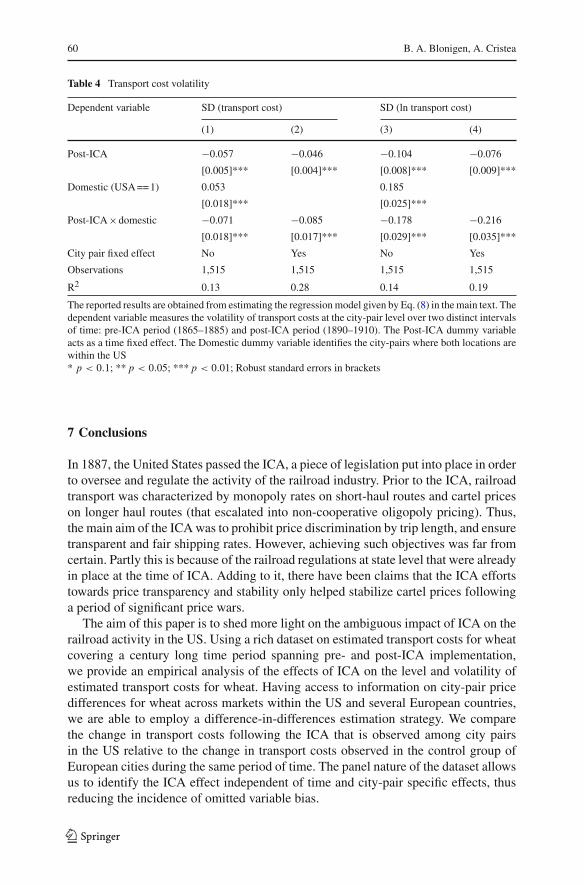
We also conduct a more formal statistical analysis of the volatility hypothesis. Wedefine volatility as the standard error over a series of transport cost values, and weconstruct two transport-cost volatility measures for each city-pair in our sample: oneover five consecutive time periods preceding the ICA (i.e., 1865–1885), and anotherover five consecutive time periods following the ICA (i.e., 1890–1910). To examinethe hypothesis that the ICA brings price stability to the railroad sector, we estimate asimple linear regression model:

V olatili t yi j,T = γ0 + γ1 Domestici j + γ2 Post I C AT + γ3(Domestici j

× Post I C AT ) + εi j t (8)

where T stands for the two time periods: pre- and post-ICA, respectively; Domestici j

is an indicator variable that is equal to one for US-only city-pairs, and zero otherwise;and Post I C AT is also an indicator variable that is equal to one for the period oftime following the ICA. We are interested in the coefficient γ3 since it measures theaverage change in the volatility of transport costs in the US relative to the rest of theworld, over the interval of time following the ICA. If the data pattern that is observed inFig. 2 is statistically significant, then we should expect γ3 to be negative and significant.

Table 4 reports the estimation results. In Columns 1 and 2, volatility is calculatedusing the initial transport cost values, while in columns 3 and 4 volatility is calculatedusing log values of transport costs. Furthermore, the estimations that are reported incolumns 2 and 4 also include city-pair fixed effects. Across all four specifications, thecoefficient on the interaction term between the post-ICA indicator and US city pairindicator is negative and highly significant. This result gives further support to theclaim that one of the main impacts of the ICA on the activity of the railroad sectorwas to stabilize freight rates.

123


Table 4 Transport cost volatility

Dependent variable SD (transport cost) SD (ln transport cost)

(1) (2) (3) (4)

Post-ICA −0.057 −0.046 −0.104 −0.076

[0.005]*** [0.004]*** [0.008]*** [0.009]***

Domestic (USA == 1) 0.053 0.185

[0.018]*** [0.025]***

Post-ICA×domestic −0.071 −0.085 −0.178 −0.216

[0.018]*** [0.017]*** [0.029]*** [0.035]***

City pair fixed effect No Yes No Yes

Observations 1,515 1,515 1,515 1,515

R2 0.13 0.28 0.14 0.19

The reported results are obtained from estimating the regression model given by Eq. (8) in the main text. Thedependent variable measures the volatility of transport costs at the city-pair level over two distinct intervalsof time: pre-ICA period (1865–1885) and post-ICA period (1890–1910). The Post-ICA dummy variableacts as a time fixed effect. The Domestic dummy variable identifies the city-pairs where both locations arewithin the US* p < 0.1; ** p < 0.05; *** p < 0.01; Robust standard errors in brackets

7 Conclusions

In 1887, the United States passed the ICA, a piece of legislation put into place in orderto oversee and regulate the activity of the railroad industry. Prior to the ICA, railroadtransport was characterized by monopoly rates on short-haul routes and cartel priceson longer haul routes (that escalated into non-cooperative oligopoly pricing). Thus,the main aim of the ICA was to prohibit price discrimination by trip length, and ensuretransparent and fair shipping rates. However, achieving such objectives was far fromcertain. Partly this is because of the railroad regulations at state level that were alreadyin place at the time of ICA. Adding to it, there have been claims that the ICA effortstowards price transparency and stability only helped stabilize cartel prices followinga period of significant price wars.

The aim of this paper is to shed more light on the ambiguous impact of ICA on therailroad activity in the US. Using a rich dataset on estimated transport costs for wheatcovering a century long time period spanning pre- and post-ICA implementation,we provide an empirical analysis of the effects of ICA on the level and volatility ofestimated transport costs for wheat. Having access to information on city-pair pricedifferences for wheat across markets within the US and several European countries,we are able to employ a difference-in-differences estimation strategy. We comparethe change in transport costs following the ICA that is observed among city pairsin the US relative to the change in transport costs observed in the control group ofEuropean cities during the same period of time. The panel nature of the dataset allowsus to identify the ICA effect independent of time and city-pair specific effects, thusreducing the incidence of omitted variable bias.

123


Our empirical analysis generates several interesting results. First, we find no sta-tistical evidence that the US transport costs experience any systematic change afterthe introduction of the ICA, on average. However, we do find that the volatility ofthe estimated shipping rates declines significantly following the ICA. This evidenceis consistent with the revisionist view that the ICA helped stabilize cartel prices aftera period of significant price wars.

Acknowledgments We thank David Jacks for sharing his data with us, and Mitch Johnson for excel-lent research assistance. We also thank Lawrence White, Wes Wilson and anonymous referees for theircomments.

8 Appendix

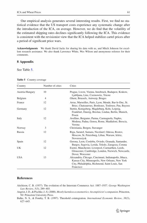
See Table 5.

Table 5 Country coverage

Country Number of cities Cities

Austria-Hungary 10 Prague, Lwow, Vienna, Innsbruck, Budapest, Krakow,Ljubljana, Linz, Czernowitz, Trieste

Belgium 4 Ghent, Brussels, Antwerp, Bruges

France 12 Arras, Marseilles, Paris, Lyon, Mende, Bar-le-Duc, St.Briec, Chateauroux, Bordeaux, Toulouse, Pau, Bayeux

Germany 12 Stettin, Konigsberg, Magdeburg, Koln, Leipzig,Frankfurt, Danzig, Breslau, Lindau, Berlin, Munich,Posen

Italy 12 Avellino, Bergamo, Parma, Carmagnola, Naples,Modena, Padua, Genoa, Rome, Maddaloni, Brescia,Verona

Norway 3 Christiania, Bergen, Stavanger

Russia 12 Riga, Saratof, Samara, Nicolaief, Odessa, Rostov,Moscow, St. Petersburg, Libau, Warsaw, Ieletz,Novorossiysk

Spain 12 Gerona, Leon, Cordoba, Oviedo, Granada, Santander,Burgos, Segovia, Lerida, Toledo, Zaragoza, Coruna

UK 12 Exeter, Manchester, Liverpool, Carmarthen, Leeds,Gloucester, Cambridge, London, Norwich, Newcastle,Dover, Worcester

USA 13 Alexandria, Chicago, Cincinnati, Indianapolis, Ithaca,Kansas City, Minneapolis, New Orleans, New YorkCity, Philadelphia, Richmond, Saint Louis, SanFrancisco

References

Aitchison, C. B. (1937). The evolution of the Interstate Commerce Act: 1887–1937. George WashingtonLaw Review, 5(3), 289–403.

Angrist, J. D., & Pischke, J.-S. (2008). Mostly harmless econometrics: An empiricist’s companion. Princeton,NJ: Princeton University Press.

Balke, N. S., & Fomby, T. B. (1997). Threshold cointegration. International Economic Review, 38(3),627–645.

123


Benson, L. (1955). Merchants, farmers, and railroads. Cambridge, MA: Harvard University Press.Binder, J. J. (1985). Measuring the effects of regulation with stock price data. RAND Journal of Economics,

16(2), 167–183.Buck, S. (1921). The Agrarian Crusade. New Haven, CT: Yale University Press.Canjels, E., Prakash-Canjels, G., & Taylor, A. M. (2004). Measuring market integration: Foreign exchange

arbitrage and the gold standard. Review of Economics and Statistics, 86(4), 868–882.Dennis, S. M. (1999). Using spatial equilibrium models to analyze transportation rates: An application to

steam coal in the United States. Transportation Research Part E: Logistics and Transportation Review,35(3), 145–154.

Donaldson, D. (Forthcoming). Railroads of the Raj: Estimating the impact of transportation infrastructure.American Economic Review.

Ejrnaes, M., & Persson, K. G. (2000). Market integration and transport costs in France 1825–1903. Explo-rations in Economic History, 37(2), 149–173.

Fogel, Robert W. (1964). Railroads and American economic growth: Essays in econometric history (Vol.296). Baltimore, MD: Johns Hopkins Press.

Gilligan, T. W., Marshall, W. J., & Weingast, B. R. (1990). The economic incidence of the InterstateCommerce Act of 1987: A theoretical and empirical analysis of the short-haul pricing constraint. RANDJournal of Economics, 21(2), 189–210.

Goodwin, B. K., & Grennes, T. J. (1998). Tsarist Russia and the world wheat market. Explorations inEconomic History, 35(4), 405–430.

Hansen, B. E. (1997). Inference in TAR models. Studies in Nonlinear Dynamics and Econometrics, 2(1),1–14.

Hansen, B. E., & Seo, B. (2002). Testing for two-regime threshold cointegration in vector error correctionmodels. Journal of Econometrics, 110(2), 293–318.

Jacks, D. S. (2005). Intra- and international commodity market integration in the Atlantic economy, 1800–1913. Explorations in Economic History, 42(3), 381–413.

Jacks, D. S. (2006). What drove 19th century commodity market integration? Explorations in EconomicHistory, 43(3), 383–412.

Kolko, G. (1965). Rails and regulation, 1877–1918. Princeton, NJ: Princeton University Press.MacAvoy, P. W. (1965). The economic effects of regulation: The trunk-line railroad cartels and the interstate

commerce commission before 1900. Cambridge, MA: The MIT Press.Meyer, B. D. (1995). Natural and quasi-natural experiments in economics. Journal of Business and Economic

Statistics, 13(2), 151–161.Miller, G. (1971). Railroads and the Granger laws. Madison, WI: University of Wisconsin Press.O’Rourke, K. H., Taylor, A. M., & Williamson, J. G. (1996). Factor price convergence in the late nineteenth

century. International Economic Review, 37(3), 499–530.Persson, K. G. (2004). Mind the gap! Transport costs and price convergence in the nineteenth century

Atlantic economy. European Review of Economic History, 8(2), 125–148.Porter, R. H. (1983). A study of cartel stability: The Joint Executive Committee, 1880–1886. Bell Journal

of Economics, 14(2), 301–314.Prager, R. A. (1989). Using stock price data to measure the effects of regulation: The Interstate Commerce

Act and the railroad industry. RAND Journal of Economics, 20(2), 280–290.Ripley, W. Z. (1906). The trunkline rate system: A distance tariff. Quarterly Journal of Economics, 20(2),

183–210.Saxonhouse, G. R. (1976). Estimated parameters as dependent variables. American Economic Review,

66(1), 178–183.Shiue, C. H., & Keller, W. (2007). Markets in China and Europe on the eve of the industrial revolution.

American Economic Review, 97(4), 1189–1216.Spann, R. M., & Erickson, E. W. (1970). The economics of railroading: The beginning of cartelization and

regulation. Bell Journal of Economics and Management Science, 1(2), 227–244.Ulen, T. S. (1980). The market for regulation: The ICC from 1887 to 1920. American Economic Review,

70(2), 306–310.Zerbe, R. (1980). The costs and benefits of early regulation of the railroads. The Bell Journal of Economics,

11(1), 343–350.

123

the effects of the interstate commerce act on...

Documents