the effects on stature of poverty, family size and birth …ftp.iza.org/dp3314.pdf · the effects...
TRANSCRIPT

IZA DP No. 3314
The Effects on Stature of Poverty, Family Sizeand Birth Order: British Children in the 1930s
Timothy J. HattonRichard M. Martin
DI
SC
US
SI
ON
PA
PE
R S
ER
IE
S
Forschungsinstitutzur Zukunft der ArbeitInstitute for the Studyof Labor
January 2008

The Effects on Stature of Poverty,
Family Size and Birth Order: British Children in the 1930s
Timothy J. Hatton University of Essex, Australian National University
and IZA
Richard M. Martin University of Bristol
Discussion Paper No. 3314 January 2008
IZA
P.O. Box 7240 53072 Bonn
Germany
Phone: +49-228-3894-0 Fax: +49-228-3894-180
E-mail: [email protected]
Any opinions expressed here are those of the author(s) and not those of IZA. Research published in this series may include views on policy, but the institute itself takes no institutional policy positions. The Institute for the Study of Labor (IZA) in Bonn is a local and virtual international research center and a place of communication between science, politics and business. IZA is an independent nonprofit organization supported by Deutsche Post World Net. The center is associated with the University of Bonn and offers a stimulating research environment through its international network, workshops and conferences, data service, project support, research visits and doctoral program. IZA engages in (i) original and internationally competitive research in all fields of labor economics, (ii) development of policy concepts, and (iii) dissemination of research results and concepts to the interested public. IZA Discussion Papers often represent preliminary work and are circulated to encourage discussion. Citation of such a paper should account for its provisional character. A revised version may be available directly from the author.
IZA Discussion Paper No. 3314 January 2008
ABSTRACT
The Effects on Stature of Poverty, Family Size and Birth Order: British Children in the 1930s*
This paper examines effects of socio-economic conditions on the standardised heights and body mass index of children in Interwar Britain. It uses the Boyd Orr cohort, a survey of predominantly poor families taken in 1937-9, which provides a unique opportunity to explore the determinants of child health in the era before the welfare state. We examine the trade-off between the quality (in the form of health outcomes) and the number of children in the family at a time when genuine poverty still existed in Britain. Our results provide strong support both for negative birth order effects and negative family size effects on the heights of children. No such effects are found for the body mass index (BMI). We find that household income per capita positively influences the heights of children but, even after accounting for this, the number of children in the family still has a negative effect on height. This latter effect is closely associated with overcrowding and particularly with the degree of cleanliness or hygiene in the household, which conditions exposure to factors predisposing to disease. We also analyse evidence collected retrospectively, which indicates that the effects of childhood conditions on height persisted into adulthood. JEL Classification: J13, I12, I31 Keywords: child health, heights, poverty Corresponding author: Timothy J. Hatton School of Economics Australian National University HW Arndt Building 25a ACT 0200 Australia E-mail: [email protected]
* We are grateful to Alison Booth for many useful conversations and comments during the writing of this paper and for comments from workshop participants at Essex and seminar participants at Warwick.
Introduction
In this paper we study the effects of per capita income, family size and birth order
on height-for-age and body mass index of children in a sample of UK households in the
1930s. We use a unique dataset from a survey conducted in 1937-9 by the Rowett
Research Institute at Aberdeen, to investigate the effects of poverty and housing
conditions on the diet and health of children. This was a time when poverty was still
widespread and when the welfare state was in its infancy. Thus we can examine these
effects for a period when the incomes of many families were low enough, and family
sizes large enough, to seriously limit the nutrition of children. We are also able to
examine directly the effects of food expenditure and housing conditions on the health of
children. Importantly, because we have data on different children within a given family
we can look into intra-family outcomes for children. And because we have evidence
from a follow up survey of members of the Boyd Orr cohort we are able to analyse the
link between childhood conditions and final attained (adult) height.
Our results provide support both for negative birth order effects and negative
family size effects on the heights of children. No such effects are found for body mass
index (BMI). We find that household income per capita positively influenced the heights
of children but even after accounting for this, the number of children in the family still
has a negative effect on height. The key mechanisms at work appear to be the positive
effect of per capita expenditure on food and a negative effect of crowding within the
household. This latter effect is closely associated with the degree of cleanliness or
hygiene in the household and we conclude that this affects height through conditioning
the exposure to disease, which in turn limits the capacity to absorb the available food
supply. Finally, we analyse information on heights recorded in the follow-up survey and
find that the effects of childhood conditions on height persisted into adulthood.
The paper is laid out as follows. A selective review of the relevant literature is
followed by an outline of a basic framework for the empirical work. We then briefly
introduce our data source, the Boyd Orr cohort. The empirical analysis begins with a
fixed effects analysis of the effect of birth order on height and BMI, and continues with a
cross-household instrumental variables analysis of the effects of family size, both in the
absence and in the presence of per capita income. The following two sections we explore
2

the mechanisms at work on child health at the household level by examining the effects
of food expenditure and housing conditions. Finally we examine the persistence of these
effects by using retrospective data to estimate the effects of childhood conditions on the
adult heights of cohort members. The results are summed up in a brief conclusion.
Background
There has been considerable interest in the effects of household composition and
socio-economic status on the welfare of children and on their later life chances. A
number of studies have investigated the effects of family size and birth order on the
outcomes for children in order to test the idea of a trade-off between the quantity and
quality of children. The essential framework is that of human capital theory, as originally
applied in a household setting by Becker and Lewis (1973) and Becker and Tomes
(1976). The basic idea is that parents obtain utility from the quantity and the quality of
children and that they maximise their utility subject to a budget constraint. Since
investment in child quality consumes resources (goods and time) there is a trade-off
along the budget constraint between the number of children and average child quality.
Most of the existing research has focused on the relationship between the number
of siblings in the family and their educational outcomes. In one of the more influential
studies Hanusheck (1992) found that the test scores for low-income families in Gary,
Indiana were inversely related to the number of children in the family but not to birth
order. More recently Booth and Kee (2007) find that the completed education-level for a
sample of British adults is inversely related to the number of siblings and also inversely
related to the individual’s birth order. In a study of young Norwegian adults, Black et al.
(2005) find strong negative birth order effects on education but no effect for family size.
By contrast, in a study of children and young adults in the Philippines, Ejrnæs and
Pörtner (2004) find a strong positive birth order effect on completed education and time
spent on school activities, although they do not investigate family size effects.
Two key methodological issues have emerged in the more recent studies. The first
is that of estimating the effects of birth order independently of family size. Since children
with low birth order will on average be from smaller families there is a natural correlation
between birth order and family size. Booth and Kee (2007) construct a birth order index
3
which is independent of family size while Black et al. (2005) estimate birth order effects
for given family sizes and Ejrnæs and Pörtner estimate across siblings using family fixed
effects. The second issue is how to estimate family size effects when family size and
child outcomes may include common unobserved effects. Booth and Kee (2007) use
region of residence and age difference between parents as instruments for the number of
children in the completed family. A number of studies including Black et al. (2005)
follow Rosenzweig and Wolpin (1980) in using the incidence of twin births on the
grounds that this is an exogenous source of variation to family size.
Although most of the existing work has focused on education as an outcome that
reflects investment in children, a number of studies have investigated the health status of
children. The trade-off between the number of children and their health status may be
particularly stark for low-income families in developing countries. One of the key
outcomes is height, which is sensitive to nutritional status, especially during early
childhood. While short stature is often interpreted as reflecting the cumulative effects
nutritional deficiency, low BMI is seen as reflecting short-run shocks to nutrition. In a
sample of children in the Philippines, Horton (1988) found strong negative effects of
birth order on height-for age but only modest effects on weight-for-height. These effects
are consistent with results on the allocation of nutrients by birth order to children in rural
India reported by Behrman (1988). A number of studies have also identified negative
family size effects on height as well as on a variety of other health indicators for children
in developing countries, although they typically do not account for the endogeneity of
family size. In one recent study of Romanian children Glick et al. (2006) find that twin
births significantly increase family size and negatively affect the standardised heights of
other siblings in the family.
Research in the UK context has focused on the National Child Development
Study (NCDS), which comprises all children born between the 3rd and 9th of March
1958.1 Li and Power (2004) find that the heights of these children at the age of 7 were
negatively related to birth order and also to the number of younger siblings as well as
being influenced by the social class of the household head and the number of persons per
1 For a wide-ranging account of trends observed in the NCDS, see Wadsworth (1991); earlier studies of height at age seven in the NCDS include Goldstein (1971) and Fogelman (1975).
4
room in the household. Interestingly, they find that these effects are generally much
smaller for the children of the original cohort, suggesting that the impact of the household
environment has become weaker as living standards have increased. The Boyd Orr cohort
used in this paper has the advantage of observing children in much poorer conditions
twenty years earlier. More important still, it provides data on a number of children in
each family, making it possible to distinguish between within- and between-family
effects.
Previous analysis by epidemiologists of the Boyd Orr cohort suggests that
demographic and economic factors were important influences on the heights of these
children (Gunnell et al., 1998a; Martin et al., 2002). One of these found that height was
negatively associated with the number of children in the household but there was no
consistent relationship between height and birth order. Other influences included the
household’s per capita expenditure on food and the degree of crowding in the dwelling.
Interestingly, these effects were found to be most important for leg length rather than
trunk length, especially for younger children (Gunnell et al., 1998a). These studies
include a wide array of explanatory variables but do not distinguish between direct and
indirect effects, and they do not account for potential endogeneity.
An important issue is whether socio-economic effects on height observed during
childhood persist into adulthood or whether retarded growth during childhood may be
compensated by catch-up growth in later adolescence. Previous studies of the Boyd Orr
cohort indicate that there is a strong correlation between measures such as height and leg
length observed during childhood and the same measures observed in adulthood (Gunnell
et al., 2000). However, these correlations are likely to capture genetic influences as well
as the ongoing effects of childhood conditions. Other analyses suggest that height during
childhood acts as a marker for the incidence of diseases such as cancer that occur later the
life-course as well as for overall mortality (Gunnell et al., 1998b, 1998c). One recent
study draws a direct link between income and housing conditions during childhood and
the longevity of members of the Boyd Orr cohort, one third of whom are now deceased.
(Frijters et al., 2007).
5
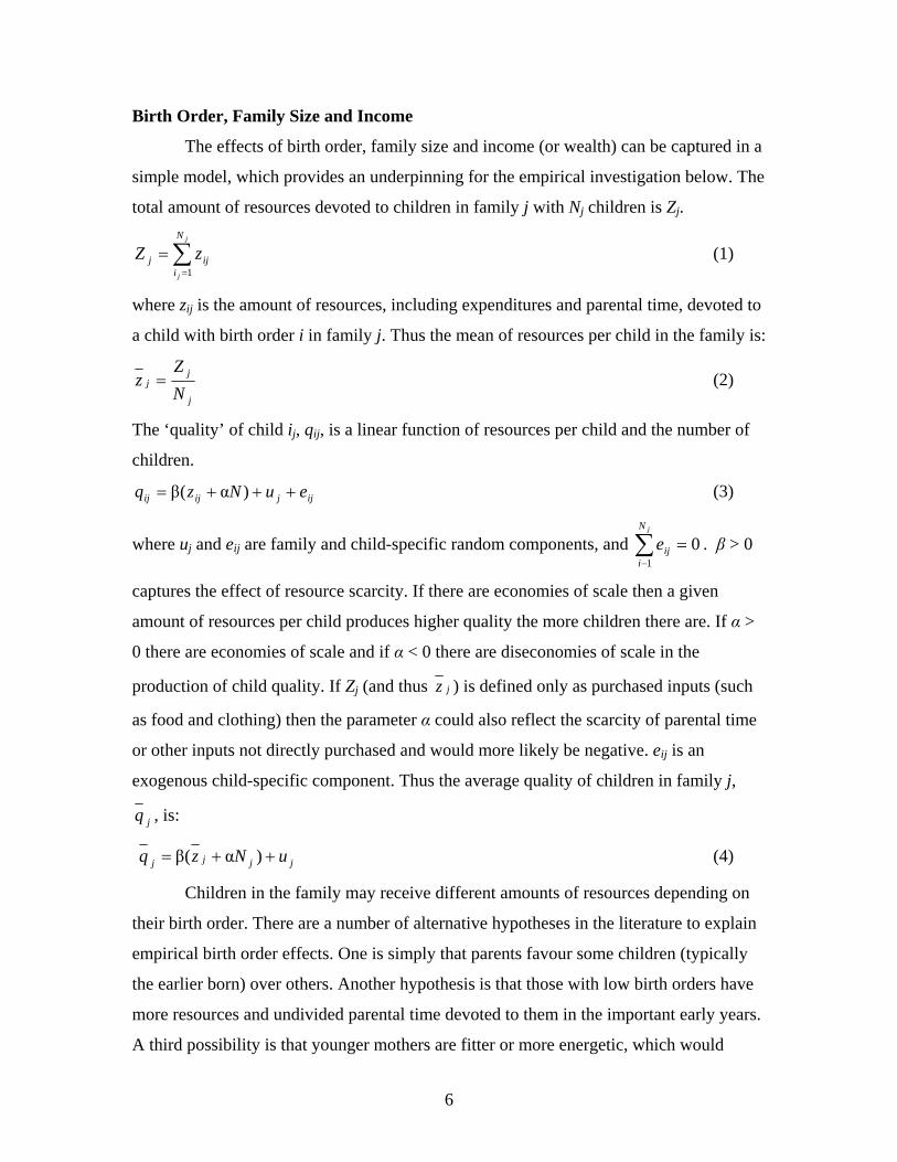
Birth Order, Family Size and Income
The effects of birth order, family size and income (or wealth) can be captured in a
simple model, which provides an underpinning for the empirical investigation below. The
total amount of resources devoted to children in family j with Nj children is Zj.
(1) ∑=
=j
j
N
iijj zZ
1
where zij is the amount of resources, including expenditures and parental time, devoted to
a child with birth order i in family j. Thus the mean of resources per child in the family is:
j
jj
NZ
z = (2)
The ‘quality’ of child ij, qij, is a linear function of resources per child and the number of
children.
ijjijij euNzq +++= )α(β (3)
where uj and eij are family and child-specific random components, and ∑ . β > 0
captures the effect of resource scarcity. If there are economies of scale then a given
amount of resources per child produces higher quality the more children there are. If α >
0 there are economies of scale and if α < 0 there are diseconomies of scale in the
production of child quality. If Z
−
=jN
iije
10
j (and thus jz ) is defined only as purchased inputs (such
as food and clothing) then the parameter α could also reflect the scarcity of parental time
or other inputs not directly purchased and would more likely be negative. eij is an
exogenous child-specific component. Thus the average quality of children in family j,
jq , is:
jjjj uNzq ++= )α(β (4)
Children in the family may receive different amounts of resources depending on
their birth order. There are a number of alternative hypotheses in the literature to explain
empirical birth order effects. One is simply that parents favour some children (typically
the earlier born) over others. Another hypothesis is that those with low birth orders have
more resources and undivided parental time devoted to them in the important early years.
A third possibility is that younger mothers are fitter or more energetic, which would
6
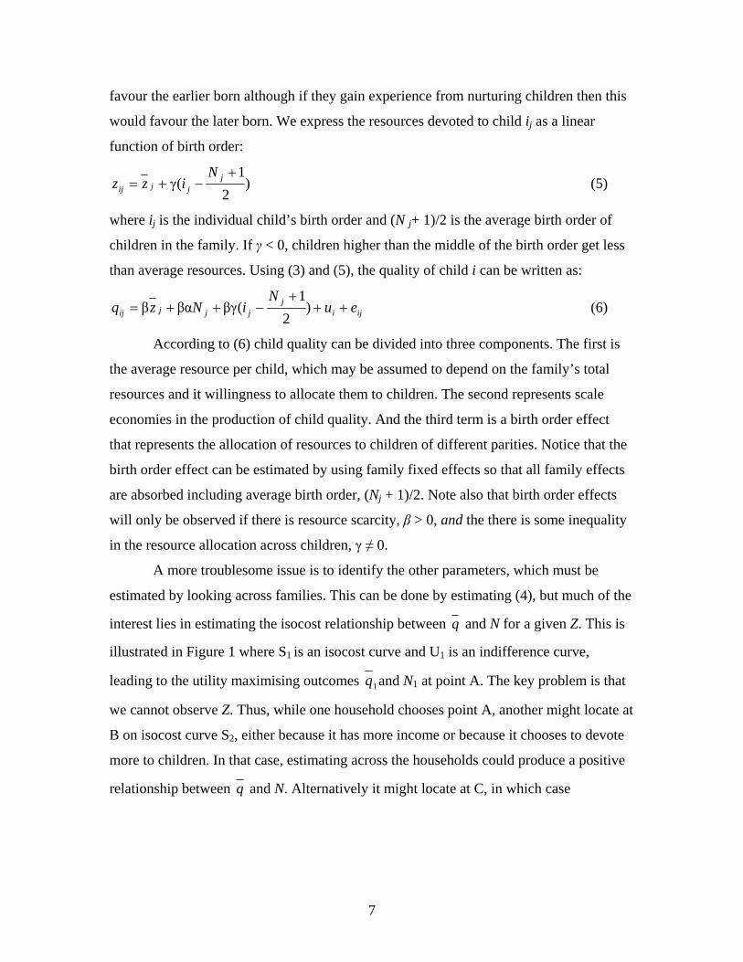
favour the earlier born although if they gain experience from nurturing children then this
would favour the later born. We express the resources devoted to child ij as a linear
function of birth order:
)2
1(γ
+−+= j
jjij
Nizz (5)
where ij is the individual child’s birth order and (N j+ 1)/2 is the average birth order of
children in the family. If γ < 0, children higher than the middle of the birth order get less
than average resources. Using (3) and (5), the quality of child i can be written as:
ijij
jjjij euN
iNzq +++
−++= )2
1(βγβαβ (6)
According to (6) child quality can be divided into three components. The first is
the average resource per child, which may be assumed to depend on the family’s total
resources and it willingness to allocate them to children. The second represents scale
economies in the production of child quality. And the third term is a birth order effect
that represents the allocation of resources to children of different parities. Notice that the
birth order effect can be estimated by using family fixed effects so that all family effects
are absorbed including average birth order, (Nj + 1)/2. Note also that birth order effects
will only be observed if there is resource scarcity, β > 0, and the there is some inequality
in the resource allocation across children, γ ≠ 0.
A more troublesome issue is to identify the other parameters, which must be
estimated by looking across families. This can be done by estimating (4), but much of the
interest lies in estimating the isocost relationship between q and N for a given Z. This is
illustrated in Figure 1 where S1 is an isocost curve and U1 is an indifference curve,
leading to the utility maximising outcomes 1q and N1 at point A. The key problem is that
we cannot observe Z. Thus, while one household chooses point A, another might locate at
B on isocost curve S2, either because it has more income or because it chooses to devote
more to children. In that case, estimating across the households could produce a positive
relationship between q and N. Alternatively it might locate at C, in which case
7

comparing A and C would produce a negative relationship. Neither would estimate the
slope of S1 and therefore the ‘true’ quality-quantity trade-off along the isocost curve.2
One solution to this problem that has appeared in the literature is to use the
incidence of twins as an exogenous shock to family size, based on the assumption that
subsequent fertility behaviour is not fully compensating. The advent of twins could shift
the household along the original isocost curve, from A to point A’, and thus it would be
an appropriate instrument. While the family could shift to a higher (or lower) isocost
curve in response to the twin-birth shock, this is likely to be a second order effect.
However there are some pitfalls in using twins as an instrument, which we discuss further
below.
Apart from the reduced form effect of family size, an important issue is how
strongly child health is related to the family’s income level and whether there are
economies of scale. We explore this by estimating equation (4) above. We also examine
whether family size has an effect on child health in addition to that working through per
capita income. In addition, we attempt to dig further into the mechanisms involved by
looking at the combined effects of food expenditure and housing conditions on the
heights of children.
Data: The Boyd Orr Cohort
The Boyd Orr survey is one of the few surveys undertaken in interwar Britain for
which the individual records survive and the only one that contains evidence on the
heights and weights of children as well as other relevant details on income, family
structure and housing conditions. The records from this study have been collected and
supplemented with additional data from follow-up surveys by a team of medical
researchers at the University of Bristol (Martin et al., 2005). The original survey included
a total of 1343 households containing children under the age of 19. A selection of
households with school-age children was surveyed in 16 towns and villages in England
and Scotland in the years 1937-9. These were intended to be representative of urban and
2 In the context of the model set out above the slope of the isocost curve is
Nqβ
−αβ2 , which is negative
provided that β > 0 and α is sufficiently small.
8

rural locations but the survey was confined to households with children and it was
targeted to over-represent poor families.3 The survey recorded details of the demographic
structure of each household together with details of income and housing conditions. It
also recorded itemised details of expenditure and consumption of food during the survey
week. Finally, the clinical part of the survey collected a variety of indicators of the
anthropometric and health status of the children including height, leg length, weight,
incidence of medical conditions and dental decay. The Bristol team conducted follow up
surveys in 1997/8 and 2002/3 of those who could be traced, collecting details on their
health and socio-economic status later in life.
The two variables that are the focus of this study are height and body mass index
(BMI)4. These were collected in the medical survey, which was conducted separately
from the initial survey of the households. The medical survey did not cover all the
households nor did it measure each child in the households that were included in the
initial survey. As compared with the original sample, the medical survey under-represents
infants, those aged 14 and over, and most important, those in certain locations.5 Here we
focus on children aged 2 to 14, for whom measurement of both height and weight is
available for a total 2946 children in 1131 households.6
The heights of these children by age are plotted in Figure 2. The heights of boys
and girls are very similar, increasing fairly linearly from about 85 cm at age 2 to 152 cm
at age 14. These can be compared with Department of Health Data for England in 2002.
As compared with current heights children in the Boyd Orr cohort were more that 6 cm
shorter by the age of 8 and more than 9cm shorter at the age of 12. Figure 3 shows the
same comparison for BMI, which follows a characteristics U-shaped pattern with a mean 3 The 16 locations are, in Scotland: Aberdeen, Kintore, Hopeman, Barthol Chapel, Methlick, Tarves, West Wemyss, Coaltown of Wemyss, Dundee and Edinburgh; and in England: Barrow-in-Furness, Liverpool, Yorkshire, Wisbech, Fulham and Bethnal Green. These locations are identified on a map in Martin et al. (2005), p. 743. 4 BMI is weight in kilograms divided by height in metres squared. 5 The survey report is somewhat vague on this point, commenting that “For various reasons all children in all surveyed families could not be examined although the attempt was made to include them all” (Rowett Institute, 1955, p. 50). One difficulty seems to have been arranging attendance at a school or clinic where measuring instruments could be used. But another seems to have been simply a matter of logistics: two of the original locations (Edinburgh and Kintore) are not represented at all in the clinical survey. 6 According to the original survey report 3762 children were examined, and the records for most of these have been found. We exclude those under age 2 and over 14 because they are underrepresented and may be subject to selection bias, and also because the height measurements for the very young children are thought to be less reliable.
9

across all ages of just over 16. By the age of 14 the mean BMI in the Boyd Orr cohort
was lower than that for contemporary children by 2.9 for boys and by 3.9 for girls.
For the purposes of analysis, the heights of children are standardised by age and
sex by calculating z-scores, which are defined as:
populationreferenceofdeviationdardtans)valuereferencemedian()valueobserved(scorez −
=−
where reference values have been calibrated on the population under study. Similarly
BMI values are converted into z-scores. Thus these variables have a mean approximately
equal to zero and standard deviations approximately equal to one. Among the children in
this sample 1.7 percent of children have z-scores for height of less than two and 2.4
percent have z-scores for BMI of less than two.
Some of the other characteristics of those who were measured are reported in
Table 1, which lists the means across individuals and the means across households. The
average age of the children is 7 years and 11 months and a little over half are female. The
average child has a birth order of 2.78 and comes from a family with 4.56 children
whereas the average family has 3.74 children. Weekly family income per capita is
available only as categorical variable, with four categories: less than 10 shillings per
week, 10-15 shillings, 15-20 shillings and greater than 20 shillings. The lowest category
was considered as living in poverty by the standards of the time. Boyd Orr (1936, p. 49)
identified those living with incomes of less than 10 shillings per week as having a food
intake that was deficient in almost every constituent while those in the next income
bracket suffered deficiencies mainly in certain minerals and vitamins. As Table 1 shows
71.6 percent of children and 59.8 percent of families are poor on this criterion. Similarly,
per capita expenditure on food is grouped into four categories: less than 5 shillings, 5-7
shillings, 7-9 shillings and greater than 9 shillings. 54.8 percent of the children and 43.6
percent of households were below the five-shilling threshold.
To put some of these figures into perspective, these families are a little larger and
substantially poorer than the average for 1930s Britain, even if we look only at
households with children. They average 5.9 persons per household as compared with 4.9
for families with children in England and Wales in 1931 (Nixon, 1935, p. 150). In his
10

survey of York (a fairly typical town) in 1936, Rowntree (1941, pp. 42, 144-149) found
that 37 percent of working class households and 43 percent of children under 14 were in
poverty—a much lower percentage than in the Boyd Orr survey.7 From a present-day
perspective, the poverty line of 10 shillings a week is roughly equivalent to 2.4 US
dollars per day in 2006. This can be compared with the World Bank’s poverty lines for
Third World countries of about 3 dollars per day for moderate poverty and about 1.5
dollars per day for extreme poverty.
The survey also collected a limited amount of information on living conditions in
the household. One is the number of persons per room. 42 percent of these households
were living in overcrowded conditions, on the widely used criterion of more than two
persons per room. The investigators also gave an assessment of the general level of
cleanliness of the dwelling, ranking a third of them as good or excellent and the
remainder moderate or poor. Only 37 percent of the dwellings possessed a flush toilet
inside with the remainder being non-flush and/or outside. Finally, nearly three-quarters of
dwellings were assessed as having good or excellent ventilation, with the rest designated
as moderate or poor. This probably reflects the overall quality of the dwelling, something
that will be discussed further below.
Birth Order Effects
We begin by looking at the effects of birth order. As previously noted a number of
studies have found that outcomes for children are determined by where the child falls in
the family birth order. The most common finding is that children with higher birth orders
have less favourable outcomes. Clearly, birth order is correlated with the number of
children in the household and it is therefore difficult to identify the separate effects of
birth order and family size in cases where only one child is sampled in each family. The
Boyd Orr data is particularly useful in this respect, not only because we observe a number
of children in each family, but also because it contains a wide range of birth orders
running from first- to eleventh-born. By including family fixed effects, all effects
7 The poverty line used by Rowntree in 1936 was based on an equivalence scale but for a family of two adults and three children it was 43s 6d exclusive of rent. Rents averaged about 9s, and so the crude per-capita poverty line would be 10s 6d.
11
common to the family, in particular the number of children and family income, are
absorbed in the fixed effects.
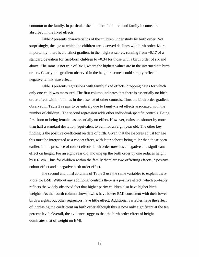
Table 2 presents characteristics of the children under study by birth order. Not
surprisingly, the age at which the children are observed declines with birth order. More
importantly, there is a distinct gradient in the height z-scores, running from +0.17 of a
standard deviation for first-born children to –0.34 for those with a birth order of six and
above. The same is not true of BMI, where the highest values are in the intermediate birth
orders. Clearly, the gradient observed in the height z-scores could simply reflect a
negative family size effect.
Table 3 presents regressions with family fixed effects, dropping cases for which
only one child was measured. The first column indicates that there is essentially no birth
order effect within families in the absence of other controls. Thus the birth order gradient
observed in Table 2 seems to be entirely due to family-level effects associated with the
number of children. The second regression adds other individual-specific controls. Being
first-born or being female has essentially no effect. However, twins are shorter by more
than half a standard deviation, equivalent to 3cm for an eight year old. The other key
finding is the positive coefficient on date of birth. Given that the z-scores adjust for age
this must be interpreted as a cohort effect, with later cohorts being taller than those born
earlier. In the presence of cohort effects, birth order now has a negative and significant
effect on height. For an eight year old, moving up the birth order by one reduces height
by 0.61cm. Thus for children within the family there are two offsetting effects: a positive
cohort effect and a negative birth order effect.
The second and third columns of Table 3 use the same variables to explain the z-
score for BMI. Without any additional controls there is a positive effect, which probably
reflects the widely observed fact that higher parity children also have higher birth
weights. As the fourth column shows, twins have lower BMI consistent with their lower
birth weights, but other regressors have little effect. Additional variables have the effect
of increasing the coefficient on birth order although this is now only significant at the ten
percent level. Overall, the evidence suggests that the birth order effect of height
dominates that of weight on BMI.
12
The results for height z-scores were subjected to a number of robustness checks.
There is no evidence of non-linearity in the birth order effects, as some hypotheses would
suggest. A full set of birth order dummies added to the second equation in Table 3 proved
to be jointly insignificant (F5, 1806 = 0.82); alternatively a squared birth order term was
insignificant (t = 0.02). The interaction of birth order and sex was insignificant (t = 0.97),
as was the interaction of poverty and birth order (t = 0.50). Thus birth order effects on
height are significantly negative, provided that cohort effects are taken into account, and
they do not seem to vary with birth order itself, with sex, or with socio-economic
conditions.
The Effect of Family Size.
One of the central issues in the literature is the effect of the number of children in
a family on their average outcomes. In order to measure the trade-off between the quality
and the quantity of children we have to look across families, and this inherently raises
issues of endogeneity. The bias will be negative if families who choose more children
also choose lower average quality, for reasons not associated with the resource constraint.
The impact of infant and child mortality, which reduces the number of children observed
in the family, is also an issue. If those who are healthiest (for reasons other than their
resource share) are more likely to survive then this selection effect leads to a negative
bias. On the other hand, families that suffer from poor health generally (and possibly
genetically) may have higher mortality and less healthy children than otherwise similar
families, leading to a positive bias. Using country-level data, Bozzoli et al. (2007) find
that the balance of these effects produces a ‘U’ shaped relationship between average
height and infant mortality. With an infant mortality rate of about 70 per thousand,
interwar Britain falls somewhere in the middle of this range, where these effects are
roughly offsetting.8
As noted previously, a popular methodology for dealing with endogeneity is to
use the incidence of twin births as an exogenous shock to family size. However, the 8 Specifically they find that the selection effect dominates at very high levels of infant mortality, so that lower mortality reduces average height. In the lower mortality environment of post-war Europe, the ‘scarring’ effect dominates so that lower mortality increases average height. From visual inspection the relationship between height and infant mortality is fairly flat in the range of mortality between 80 and 200 per thousand (Bozzoli et al., 2007, Figure 6).
13
incidence across families of any twin birth is endogenous since it is a function of the
number of births, and hence of family size, and so the literature typically uses twin births
at a given parity. Here we use twins at last birth (rather than at first birth) for three
reasons. One is that with the relatively large family sizes in this dataset last birth will
have a greater influence on family size than births at lower parities. Second, and perhaps
related, there are more twin last births than first births, which is an important
consideration given that twin birth is a rare event. Third, since the birth of twins might
have a direct effect on higher parity children (and not just an effect working through
family size), this ensures that we focus on those with lower parities than the twins that are
used to derive the instrument.
Table 4 presents estimates for the effects of the number of children on height
using the family as the unit of observation. This means that the height on the left hand
side is the average z-score of measured children in each family, excluding twins, and thus
eliminating the twins that are used to create the instrument.9 We also include the average
date of birth to capture the cohort effect, but we exclude birth order since, as noted
earlier, average birth order is simply a linear function of the number of children, which is
therefore a size effect. The ordinary least squares coefficient in the first column on the
number of children is negative and highly significant with a coefficient of –0.13. The
instrumental variables coefficient in the second column, using twins as the only
instrument, is more negative at –0.23. Thus the OLS coefficient appears to be an
underestimate of the true (negative) effect, although the test for endogeneity is not
significant.10 The IV coefficient in the second column implies that adding one child to the
family reduces height at age eight by 1.2cm.
It is worth examining the combined effect of family size and birth order across
different children. If dilution of resources is a key determinant of height then height
should decline with both birth order and family size. Thus, for the first child in the family
the (negative) family size effect of adding one more child should exceed the (positive)
9 Note that because average height is not calculated over all the children in each family this measure could be biased if high or low birth order children were underrepresented. Comparing the average birth order by family from Table 1 (2.35) with that which would be predicted from average the number of children ((3.74 + 1)/2 = 2.37) indicates that this is not a serious concern. 10 Although the incidence of twins is low this variable passes the weak instrument test, with an F-statistic for the first stage regression of 20.2.
14

effect of increasing the gap between the first child’s birth order and the mean birth order.
These effects are plotted in Figure 4, based on the coefficients in Col. 2 of Table 3 and
Col. 2 of Table 4. The predicted values are plotted as deviations from the predicted height
of the third child in a five-child family (for which the value is set to zero). Relative to this
benchmark, an only child is taller by 0.92 of a standard deviation while the first child in a
nine-child family is shorter by 0.50 of a standard deviation. The total family size effect
between first children in one- and nine-child families equates to as much as 12cm at age
14. Thus adding more children has a strong negative effect on the heights of the
preceding children. The birth order effects are slightly smaller, with a gap at age 14
between the first and ninth child of 0.97 of a standard deviation or about 7cm.
For what follows below it is also worth exploring estimates with additional
instruments. The first is a set of 14 location dummies. The correlation between fertility
and locality is quite strong and there is a historical literature that points to distinct
regional differences in fertility. For 1911 and earlier Garrett et al. (2001) find distinct
differences in completed family size associated with urban and rural settings and with the
industrial character of the locality. They argue that this reflects differences in spatial
evolution of social norms.11 These neighbourhood effects are useful as instruments
because they abstract from family-level heterogeneity. The second is a set of dummies for
social class (6 categories based on occupation), which the historical literature also
identifies as a key determinant of family size.12 Social class is very strongly correlated
with income, but because it is less subject to short-term shocks, it may be thought of as
closer to permanent income, which would be more appropriate as a determinant of long-
term health status than would be the case for current income. 11 Garrett et al. comment that “Individuals did not necessarily have to talk to one another about fertility per se in order to reflect upon how to behave with regards to family size: by observation of their neighbours in myriad daily interactions in public places such as the street, the church and the workplace people realised that smaller families had advantages, or conversely, that large families were becoming an object of pity. Each couple would have conceptualised these advantages in their own terms: some may have understood that fewer children meant more money to spend per member of the household; others might have realised the dividends to be gained in terms of health; or perhaps they simply came to recognise that large families were something, which, somehow, the respected and the respectable in their community deemed it prudent to avoid” (2001, p. 289). For an account of household decisions on fertility in the interwar period based on oral history, see Gittins (1982). 12 See for example the study of occupation and fertility in1889/90 by Haines (1979). More recent studies of the late nineteenth century fertility decline have stressed that the relationship between occupation and fertility is only imperfectly captured by the broad aggregation into social classes and that a number of other influences (such as locality) are equally important correlates of fertility (Szreter, 1996; Garrett et al., 2001)
15

The third column of Table 4 uses twins and locality dummies as instruments and
this substantially increases the significance of the family size coefficient as compared
with using only twins. Interestingly, the coefficient is exactly the same as that using the
twin instrument alone. The fourth column adds social class to the instrument set and this
further raises the significance of the family size coefficient, which now becomes
marginally more negative. The first stage estimates using this full instrument set are
reported in the Appendix. We have to be careful about adding instruments that could in
principle be correlated with the error term in the equation. Given the limited number of
explanatory variables it is not surprising that the estimates in the third and fourth columns
fail the overidentification test. But the important point is that adding additional
instruments does not bias the coefficient back towards the OLS estimate. In these
estimates date of birth is negative, in contrast with the result for birth order in Table 3,
but it is insignificant in every case.
Table 5 repeats this exercise on the BMI index. The OLS estimate suggests that
family size has no effect on BMI across families. Although the coefficient is always
positive it is never significant with any of the instrument sets. This seems to be consistent
with the results for birth order in the sense that that resource scarcity has stronger effects
on height than on BMI. These findings suggest that the effects measured here are long-
term cumulative effects, which are usually associated with height, rather than short-term
shocks to nutrition, which are more often associated with weight-for-height.
The estimates in Table 4 were subject to a number of robustness checks. One
concern is that family size is measured with error because we only observe the number of
children currently in the household and not completed family size. This is less of a
concern for health status observed currently (which is influenced largely by conditions at
the time) than for outcomes such as completed education that are observed much later.
However, later children in older families may be living with fewer siblings than when
they were in their infancy. In order to explore this we re-estimated the equations for
heights in Table 4 using a sample of households in which there was at least one child
under eight. The coefficient estimates (‘t’ statistics) on the number of children for the
same four equations in this reduced sample of 867 observations were, respectively: –
0.113 (6.26), –0.313 (1.74), –0.244 (5.14) and –0.304 (6.60).
16

A further possible concern is that the family size effect might vary across the birth
order. Estimating the OLS coefficient equivalent to the first column of Table 4 across
individuals at a given birth order produced the following coefficients (‘t’ statistics): parity
1: –0.134 (5.21); parity 2: –0.193 (8.08); parity 3: –0.123 (4.16); parity 4: –0.115 (2.57).
Alternatively, using the full set of instruments (as in the forth column of Table 4) yielded
the following results: parity 1: –0.242 (4.57); parity 2: –0.305 (5.70); parity 3: –0.459
(6.06); parity 4: –0.306 (3.23). Thus the family size effect is negative and significant at
each birth order for which we have a reasonable number of observations, with no strong
trend across birth orders.
The Effects of Per-capita Income and Family Size
Studies of the effects of family size on the outcomes for children invoke resource
scarcity within the family as the key mechanism. That raises the question of whether the
family size effect works solely through spreading income more thinly or whether there
are additional effects, possibly arising from economies or diseconomies of scale. Thus we
estimate height outcomes for children by including per capita income in the household
and the number of children as separate regressors. To the extent that the appropriate
equivalence scale gives less than full weight to children, per capita income
underestimates the weighted per capita income by a larger margin the more children there
are. Hence we should pick up economies of scale that arise from larger family size
through a positive family size coefficient. If we find that the family size effect is negative
even in the presence of (non-equivalised) per capita income then that would strengthen
the conclusion that there are negative family size effects independent of their effects
through income per capita. As mentioned earlier, per capita income is reported in the
original survey only as a categorical variable. Since per capita income is likely to be
endogenous, we instrument this too, using the full instrument set.
Cross-household results for height and BMI z-scores are reported in Table 6. As
before, the dependent variable is the household average, and the IV estimates presented
here use the full set of instruments. The first column of Table 6 reports the OLS estimate
for standardised heights. Here, the coefficient on per capita income is positive as
expected and the coefficient on the number of children is negative. The IV estimate in the
17

second column produces a similar coefficient on per capita income and a more negative
coefficient on the number of children, consistent with our earlier results. Thus it appears
that family size has a direct negative effect on children’s heights in addition to its effect
through per capita income. If there are economies of scale in the number of children (as is
implied by most equivalence scales) then this coefficient underestimates the direct
negative effect of family size.
The third and fourth columns of the table show that the z-score for BMI is not
significantly affected by either income per capita or by the number of children. Thus
family income and demographics affect the overall size of children as reflected in height
but not their proportions as reflected in BMI. This is consistent with the results of other
regressions (not reported here) showing that both leg length and trunk length are
influenced by income per capita and the number of children.
The Effects of Food Expenditure and Housing Conditions.
Socio-economic conditions are often thought to influence the heights of children
through two key channels: food consumption and housing conditions. In order to explore
this more fully, Table 7 explains variations in height across households by food
expenditure per capita and crowding. As with income, food expenditure is available only
as a categorical variable in the original survey data, while the measure of crowding is the
number of persons per room. The first column of Table 7 illustrates the effect of these
variables across households, using the same instruments as in Table 6 (see Appendix
Table for the first stage estimates) and dropping the insignificant birth date variable. Not
surprisingly, per capita food expenditure has a positive coefficient that is consistent with
the income effect observed in Table 6. Overcrowding has a significant negative effect as
might be expected. The second column shows that when the number of children is added
as a regressor (and also treated as endogenous) it is insignificant while the coefficient on
the crowding variable remains significant. Thus it seems to be crowding rather than the
number of children per se that affects the height of children.
The last two columns of Table 7 include an additional variable that ranks the level
of cleanliness in the household, where 1 = poor, 2 = fair/moderate and 3 =
good/excellent. This variable is also instrumented. As the third column shows, it has an
18

important influence and in its presence the coefficient on persons per room becomes
small and insignificant. In the last column the presence of this variable weakens the
effects of both per capita food expenditure and the number of children. This result
supports the idea that health is influenced not only by food intake but also by the disease
environment. It widely recognised that illnesses such as diarrhoea and respiratory
infections that are common in childhood can arrest growth by limiting the absorptive
functions of the digestive tract or by reducing the individual’s appetite (for a survey of
these effects see Silventoinen, 2003). Repeated infection may have a cumulative effect
on height, particularly when food supply is limited. The effect of cleanliness is of course
indirect, but lack of hygiene is likely to reflect the presence of pathogens and an
environment conducive to the transmission of infections. The inclusion of cleanliness has
a smaller effect on the coefficient on the number of children in the fourth column than it
does on overcrowding in the third column.
In order to explore this issue a little further Table 8 provides some evidence on
the correlates of cleanliness. These are ordered probit regressions for the three values of
cleanliness, and the results should not be interpreted as causal. The first column shows
that cleanliness is inversely related to the degree of crowding, and the second column
indicates that it is also positively associated with per capita income. It seems likely that
the larger is the family and the lower is its income the more difficult it would have been
to maintain high standards of cleanliness. The third column adds a variable on toilet
facilities as an indicator of housing quality, where 1 = no flush toilet, 2 = flush toilet
outside or shared, and 3 = flush toilet inside and not shared. As the third column of Table
8 shows, this takes a positive coefficient with modest effects on the other variables.
The final column of Table 8 adds a variable for the quality of ventilation: 1 =
poor, 2 = fair/moderate, and 3 = good/excellent. This variable is highly significant and
seriously undermines the significance of the other variables. It is doubtful that this
captures only the effects of better air circulation. It seems much more likely that this
variable represents housing quality more generally, distinguishing, for instance, between
dark dingy tenements and conditions in more modern housing.13 Overall, the results
13 Other social surveys undertaken in the 1930s provide some insight into working class housing conditions and their relation to health. In his 1936 social survey of York, Rowntree classified housing quality into five
19

suggest that child health is determined through two main mechanisms. One is the food
budget relative to the number of mouths to feed. The other is the size of the family
relative to housing conditions, which influences the standard of hygiene and hence the
degree of exposure to recurrent illness for the children in the family. This latter effect is
captured by the degree of general cleanliness in the home, which may be mitigated or
exacerbated by the quality of housing.
Adult Heights and Family Size
An important question is whether the effects of childhood conditions on health
persisted into adulthood. The effects on stature might have been modified by a
compensating growth spurt during the later teenage years, an effect that might also be
conditioned by the income effect of entering the labour market. In order to examine this
issue we use data from the follow-up survey of the members of the Boyd Orr cohort who
could be traced in 1997/8. Of the 3182 who were traced, 1647 responded to a
questionnaire that included questions on health and socio-economic status during the
subsequent life-course (see Martin et al. 2005 for details of the follow-up survey). Here
we focus on a question about the individual’s height at the age of 20.
The use of data from a retrospective survey raises issues of measurement and
selection. Individuals were asked to recall their height at the age of 20 when they were in
their mid-fifties to mid-seventies. While self reported heights are typically subject to an
upward bias, extensive analysis of the adult heights reported by members of the Boyd Orr
cohort suggest that measurement error does not invalidate the usefulness of these data.14
categories. Of the worst category (occupied by about 30 percent of the working class population he commented that: “Many of them should be demolished; the rest should be improved. At present they menace the health of the occupants (Rowntree, 1941, p. 246). Lack of light and poor ventilation was a characteristic of some tenements as well as the older back-to-back houses. Many others built in Victorian times had back additions or a narrow rear access that restricted light and ventilation (this style was largely discontinued after the first World War). These conditions were often combined with a damp environment (due to the absence of damp courses) and a crumbling interior fabric. The effects of these factors are well described in the New Survey of London Life and Labour, conducted in 1929-31: “Dilapidated woodwork, plaster and wallpaper, if less serious than structural faults, are also more general. Few except the most modern working class dwellings are entirely from these defects. They are responsible for much dirt and discomfort and for the depressing atmosphere of squalor associated with so many working class homes. Their most serious effect, however, is that they harbour vermin of all sorts and especially bugs. ….[which] are a grave menace to comfort, health and peace of mind” (Llewellyn Smith (ed.) 1934, p. 188). 14 Gunnell et al. (2000) conducted clinical examinations of 138 of those who responded to the questionnaire. They found that self-reported current height exceeded measured height by 2.4 cm for 59 men
20
It is important to note that of the 1339 survey members for whom we have self-reported
height at age 20, only 866 were also measured as children. Among these the correlation
coefficient between the z-score for adult height (adjusted only for sex) and the z-score for
height during childhood is 0.67. Thus the mapping between childhood height and adult
height is attenuated by some combination of measurement error and intervening
conditions.
The characteristics during childhood of those who reported adult height are
reported in Table 9. Not surprisingly they are somewhat younger than those represented
in Table 1. They are less often from households with low income and poor housing
conditions, but the differences between the means reported in Table 9 and in Table 1 are
small. This suggests that selection bias is unlikely to be important. In initial estimates for
the effect of the number of children on adult height we estimated a selection model with a
first stage probit for inclusion in the sample. Since the inverse Mills ratio never proved
significant in the second stage regression for height we concluded that selection bias is
not important.
Table 10 reports a set of IV regressions comparable to some of those in Tables 4,
7 and 8 using the z-score for adult height as the dependent variable and using the full set
of instruments discussed earlier. The first equation illustrates that family size influences
adult height and with a coefficient about two-thirds the size of that reported in the last
column of Table 4. When per capita income is added in the second column the separate
family size effect falls to a value similar to that in Table 6. However, the coefficient on
per capita income is smaller and it is now significant only at the 10 percent level. When
food expenditure per capita is included instead of income as in the third column the
coefficient is small and insignificant. This seems to reflect the fact that, with fewer
observations and with a less accurate measure of height, it is harder to distinguish the
separate effects of income and family size. Using per capita income alone produces a
coefficient of 0.240 (‘z’ = 4.9) while per capita expenditure alone produces a coefficient
of 0.218 (‘z’ = 4.4).
and by 2.1 cm for 79 women. However, the correlation coefficient between measured and self-reported height was 0.94 for men and 0.88 for women.
21
The last column of Table 10 introduces the index of cleanliness, which was found
to be important for the health of children. The coefficient is smaller than that in the last
column of Table 7 and it is not significant. Thus while the negative effect of family size
seems to persist into adulthood the other effects are weaker when estimated in
combination. Although the effects are less precisely estimated for the Boyd Orr cohort as
adults, overall the evidence suggests that some of the effects observed during childhood
persisted into adulthood.
A similar exercise was undertaken for BMI at age 20, although we do not report
the results in full. Of the 1298 cases for whom we have self-reported BMI at age 20, 841
were also measured as children, and the correlation between the z-scores for adult BMI
and childhood BMI is 0.36. Not surprisingly, this is much lower than the correlation
between childhood and adult heights. As with BMI during childhood the effect of the
number of children is insignificant (‘z’ = 0.4) when estimated alone, and both the number
of children and family income are insignificant (‘z’ = 0.7 and 1.0) when estimated in
combination. While these results are consistent with those obtained for childhood BMI,
the degree of persistence is much lower and the likelihood of measurement error is
probably greater.
Conclusion
This paper contributes to the debate on the determinants of child quality using a
unique dataset from 1930s Britain. It focuses on child health, as reflected by standardised
height and BMI, in a sample of relatively poor households. We find that birth order and
the number of children both have strong negative effects on height but not on BMI. These
results are consistent with an interpretation that stresses the consequences of resource
dilution within and between households. The development literature often interprets
height as reflecting enduring deprivation (as it is cumulative) while BMI is typically
associated with short-run privations. On that interpretation, the effects measured here
capture the longer-term effects, which are likely to have prevailed throughout the
childhood of those in the survey.
A question less often posed is whether there is a negative family size beyond that
of simply diluting family income per capita, and if so, what mechanisms it represents.
22
Our answer to the first question is that the number of children does have an independent
negative effect and one that appears to be associated with the degree of crowding within
the household. Our answer to the second question is suggestive rather than definitive. We
find that the degree of cleanliness is important, a variable that is likely to be associated
the standard of hygiene and thus with the disease environment within the household. This
in turn is negatively associated with the degree of crowding in the household and
positively with income per capita. Better quality housing seems to reduce the effect of
crowding on height, presumably through its effects on hygiene. Thus the two key
channels though which the number of children in a family status affects the health of
children is directly through the reduction on food intake and more indirectly though the
effect of crowding via the level of hygiene on the incidence of disease.
Finally, there is evidence that these effects observed for children in the 1930s
persisted into adulthood. Although our evidence here is less precise, it appears that
poverty family size and housing conditions influenced the height and the health of the
generation of those who were prime-age adults in the early postwar period. These
findings are consistent with other evidence showing that childhood height is a marker for
bio-physiological processes that can affect future health. Reduced height is associated
with increased risk of heart disease and stroke, the major causes of death in this cohort.
23

References Becker, G. S. and Lewis, H. G. (1973), “On the Interaction between the Quantity and
Quality of Children,” Journal of Political Economy, 81, pp. S279-S288. Becker, G. S. and Tomes, N. (1976), Child Endowments and the Quantity and Quality of
Children,” Journal of Political Economy, 84, pp. S143-S162. Behrman, J, (1988), Nutrition, Health, Birth Order and Seasonality: Intrahousehold Allocation Among Children in Rural India,” Journal of Development Economics,
28, pp. 43-62. Black, S. E., Devereaux, P. J. and Salvanes, (2005), “The More the Merrier? The Effect
Family Size and Birth Order on Children’s Education,” (2005), Quarterly Journal of Economics, 120, pp. 669-700.
Booth, A. L. and Kee, H. J. (2007), “Birth Order Matters: The Effect of Family Size and Birth Order on Educational Attainment,” Revised version of IZA Discussion Paper 1713.
Boyd Orr, J. (1936), Food Health and Income: A Survey of Adequacy of Diet in Relation to Income, London: Macmillan.
Bozzoli, C., Deaton, A. S. and Quintana-Domeque (2007), “Child Mortality, Income and Adult Height,” NBER Working Paper 12966, Boston: NBER.
Ejrnæs, M. and Pörtner, (2004) “Birth Order and the Intrahousehold Allocation of Time and Education,” Review of Economics and Statistics, 86, pp. 1008-1019.
Fogelman, K. R. (1975), “Developmental Correlates of Family Size,” British Journal of Social Work, 5, pp. 43-57.
Frijters, P., Shields, M. A., Hatton, T. J. and Martin, R. M. (2007), “Childhood Economic Conditions and Length of Life: Evidence from the UK Boyd Orr Cohort, 1937– 2005,” IZA Discussion Paper 3042: Bonn: IZA
Garrett, E, Reid, A., Schürer, K. and Szreter, S. (2001), Changing Family Size in England and Wales: Place, Class and Demography, 1891, 1911. Cambridge: Cambridge University Press.
Gittins, D. (1982), Fair Sex: Family Size and Structure, 1910-39, London: Hutchinson. Glick, P. J., Marini, A. and Sahn, E. (2006), “Estimating the Consequences of
Unintended Fertility for Child Health and Education in Romania: An Analysis using Twins Data,” Cornell University: unpublished.
Goldstein, H. (1971), Factors Influencing the Height of Seven Year Old Children: Results from The National Child Development Study, Human Biology, 43, pp. 92-111.
Gunnell, D. J., Davey Smith, G., Frenkel, S. J. Kemp, M. and Peters, T. J. (1998a), “Socio-economic and Dietary Influences on Leg Length and Trunk Length in Childhood: A Reanalysis of the Carnegie (Boyd Orr) Survey of Diet and Health in Prewar Britain,” Paediatric and Perinatal Epidemiology, 12, pp. 96-113.
Gunnell, D., Davey Smith, G., Holly, J. M. P. and Frankel, S. (1998b), “Leg Length and Risk of Cancer in the Boyd Orr Cohort,” British Medical Journal, 317, pp. 1350-1.
Gunnell, D., Davey Smith, G., Frankel, S., Nanchahal, K., Braddon, F. E., Pemberton, J. and Peters, T. J. (1998c), “Childhood Leg Length and Adult Mortality: Follow up of the Carnegie (Boyd Orr) Survey of Diet and Health in Pre-War Britain,” Journal of Epidemiology and Community Health, 52, pp. 142-152.
24

Gunnell, D., Berney, L., Holland, P., Maynard, M., Blane, D., Frankel, S., and Davey Smith, G. (2000), “How Accurately are Height, Weight and Leg Length Reported by the Elderly, and How Closely are they Related to Measurements Recorded in Childhood?” International Journal of Epidemiology, 29, pp. 456-464.
Haines, M. R. (1979), Fertility and Occupation: Population Patterns in Industrialization, New York: Academic Press.
Hanusheck, E. (1992), “The Trade-off between Child Quality and Quantity,” Journal of Political Economy, 100, pp. 894-117.
Horton, S. (1988), “Birth Order and Child Nutritional Status: Evidence from the Philippines,” Economic Development and Cultural Change, 36, pp. 341-354.
Lewellyn Smith, H (ed.) (1934), The New Survey of London Life and Labour, Vol. VI, London: Longmans Green.
Li, L. and Power, C. (2004), Influences on Childhood Height: Comparing Two Generations in the 1958 British Birth Cohort,” International Journal of Epidemiology, 33, pp. 1320-1328.
Martin, R. M. (2002) Association Between Breastfeeding and Growth: The Boyd Orr Cohort Study,” Archives of Disease in Childhood: Fetal and Neonatal Edition, (2002),” 87, pp. F193-F201.
Martin, R. M., Gunnell, D., Pemberton, J., Frankel, S. and Davey Smith, G. (2005), “Cohort Profile: The Boyd Orr Cohort - An Historical Cohort Study Based on the 65 Year Follow-up of the Carnegie Survey of Diet and Health (1937-39),” International Journal of Epidemiology, 34, pp. 742-749.
Nixon, J. W. (1935), “The Size, Constitution and Housing Standards of the Family in England and Wales, 1911 to 1931,” Review of the International Statistical
Institute, 3, pp. 142-162. Rosenzweig, M. R. and Wolpin, K. I. (1980), “Testing the Quantity-Quality Fertility
Model: The Use of Twins as a Natural Experiment,” Econometrica, 48, pp. 222- 240.
Rosenzweig, M. R. and Zhang, (2006), “Do Population Policies Induce more Human Capital Investment? Twins, Birthweight and China’s ‘One Child’ Policy,” Bonn: IZA Discussion Paper 2082.
Rowett Institute (1955), Family Diet and Health in Pre-War Britain: A Dietary and Clinical Survey, Dunfermline: Carnegie U. K. Trust.
Rowntree, B. S. (1941), Poverty and Progress: A Second Social Survey of York, London: Longmans Green.
Silventionen, K. (2003), “Determinants of Variation in Adult Body Height,” Journal of Biosocial Science, 35, pp. 263-285.
Szreter, S. (1996), Fertility, Class and Gender In Britain, 1860-1940, Cambridge: Cambridge University Press.
Thomas, D. (1994), “Like Father like Son; like Mother like Daughter: Parental Resources and Child Height,” Journal of Human Resources, 29, pp. 950-988.
Wadsworth, M. E. J. (1991), Childhood, History and Adult Life, Oxford: Clarendon Press.
25

Table 1 Characteristics of Children who were Measured in the Boyd Orr Survey
By individual By Household No of cases 2946 1131Individual characteristics Average age 7.92 7.85Average birth order 2.78 2.35Percent female 52.7 53.9Household characteristics Number of children in family 4.56 3.74Family size 6.75 5.96Family income per capita < 10s 71.56 59.8Food expenditure per capita < 5s 54.75 43.50Persons per room > 2 43.76 42.01Clean house 32.26 33.11Flush toilet inside 35.40 37.00Good ventilation 70.56 73.00 Note: due to missing data some of the means are calculated on a smaller number of observations as follows (individuals, households): income per capita (2911, 1112), persons per room (2605, 984), clean house (2734, 1045), flush toilet (2099, 786) good ventilation (2707, 1037).
Table 2 Children Measured in the Boyd Orr Survey by Birth Order
Birth Order No of
Children Average age Percent
female Height z-score
BMI index z-score
1 760 9.40 54.9 0.167 -0.0442 761 8.61 50.0 0.084 0.0133 595 7.72 53.9 -0.094 0.0064 390 6.68 51.2 -0.066 0.0935 229 6.10 58.2 -0.167 0.0786+ 211 4.89 48.4 -0.340 -0.011All 2946 7.92 52.8 -0.000 0.011
26
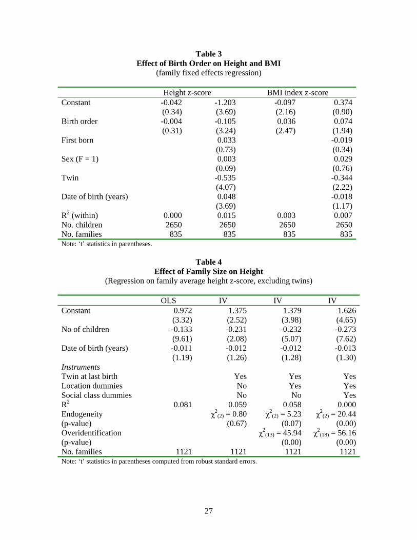
Table 3 Effect of Birth Order on Height and BMI
(family fixed effects regression) Height z-score BMI index z-score Constant -0.042 -1.203 -0.097 0.374 (0.34) (3.69) (2.16) (0.90)Birth order -0.004 -0.105 0.036 0.074 (0.31) (3.24) (2.47) (1.94)First born 0.033 -0.019 (0.73) (0.34)Sex (F = 1) 0.003 0.029 (0.09) (0.76)Twin -0.535 -0.344 (4.07) (2.22)Date of birth (years) 0.048 -0.018 (3.69) (1.17)R2 (within) 0.000 0.015 0.003 0.007No. children 2650 2650 2650 2650No. families 835 835 835 835Note: ‘t’ statistics in parentheses.
Table 4
Effect of Family Size on Height (Regression on family average height z-score, excluding twins)
OLS IV IV IV Constant 0.972 1.375 1.379 1.626 (3.32) (2.52) (3.98) (4.65)No of children -0.133 -0.231 -0.232 -0.273 (9.61) (2.08) (5.07) (7.62)Date of birth (years) -0.011 -0.012 -0.012 -0.013 (1.19) (1.26) (1.28) (1.30)Instruments Twin at last birth Yes Yes YesLocation dummies No Yes YesSocial class dummies No No YesR2 0.081 0.059 0.058 0.000Endogeneity χ2
(2) = 0.80 χ2(2) = 5.23 χ2
(2) = 20.44 (p-value) (0.67) (0.07) (0.00)Overidentification χ2
(13) = 45.94 χ2(18) = 56.16
(p-value) (0.00) (0.00)No. families 1121 1121 1121 1121Note: ‘t’ statistics in parentheses computed from robust standard errors.
27

Table 5 Effect of Family Size on Body Mass Index
(Regression on family average BMI z-score, excluding twins) OLS IV IV IV Constant 0.623 -0.123 0.446 0.561 (2.00) (0.19) (1.25) (1.63)No of children 0.010 0.192 0.053 0.025 (0.79) (1.40) (1.23) (0.72)Date of birth (years) -0.021 -0.019 -0.021 -0.021 (2.06) (1.76) (2.01) (2.05)Instruments Twin at last birth Yes Yes YesLocation dummies No Yes YesSocial class dummies No No YesR2 0.005 0.000 0.000 0.005Endogeneity χ2
(2) = 1.82 χ2(2) = 1.15 χ2
(2) = 0.15 (p-value) (0.40) (0.56) (0.93)Overidentification χ2
(13) = 39.77 χ2(18) = 44.57
(p-value) (0.00) (0.00)No. families 1121 1121 1121 1121Note: ‘t’ statistics in parentheses computed from robust standard errors.
Table 6
Effect of Income and Family Size on Height and BMI (Regression on family average height and BMI z-scores, excluding twins)
Height z-score BMI index z-score OLS IV OLS IV Constant -0.322 -0.054 0.452 0.330 (0.98) (0.11) (1.33) (0.64)Income per capita 0.265 0.275 0.035 0.035 (8.41) (4.62) (1.08) (0.52)No of children -0.071 -0.144 0.018 0.047 (4.78) (2.80) (1.31) (0.95)Date of birth (years) 0.009 0.009 -0.018 -0.018 (0.96) (0.85) (1.76) (1.60)R2 0.145 0.134 0.006 0.003Endogeneity χ2
(3) = 7.54 χ2(2) = 0.86
(p-value) (0.06) (0.83)Overidentification χ2
(17) = 46.34 χ2(18) = 42.46
(p-value) (0.00) (0.00)No. Families 1102 1102 1102 1102Note: ‘t’ statistics in parentheses computed from robust standard errors.
28
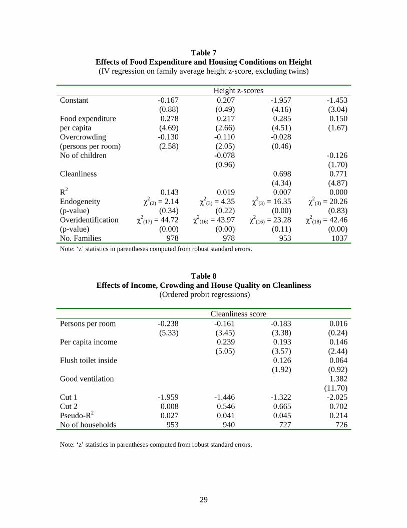
Table 7 Effects of Food Expenditure and Housing Conditions on Height (IV regression on family average height z-score, excluding twins)
Height z-scores Constant -0.167 0.207 -1.957 -1.453 (0.88) (0.49) (4.16) (3.04)Food expenditure 0.278 0.217 0.285 0.150per capita (4.69) (2.66) (4.51) (1.67)Overcrowding -0.130 -0.110 -0.028 (persons per room) (2.58) (2.05) (0.46) No of children -0.078 -0.126 (0.96) (1.70)Cleanliness 0.698 0.771 (4.34) (4.87)R2 0.143 0.019 0.007 0.000Endogeneity χ2
(2) = 2.14 χ2(3) = 4.35 χ2
(3) = 16.35 χ2(3) = 20.26
(p-value) (0.34) (0.22) (0.00) (0.83)Overidentification χ2
(17) = 44.72 χ2(16) = 43.97 χ2
(16) = 23.28 χ2(18) = 42.46
(p-value) (0.00) (0.00) (0.11) (0.00)No. Families 978 978 953 1037Note: ‘z’ statistics in parentheses computed from robust standard errors.
Table 8 Effects of Income, Crowding and House Quality on Cleanliness
(Ordered probit regressions) Cleanliness score Persons per room -0.238 -0.161 -0.183 0.016 (5.33) (3.45) (3.38) (0.24)Per capita income 0.239 0.193 0.146 (5.05) (3.57) (2.44)Flush toilet inside 0.126 0.064 (1.92) (0.92)Good ventilation 1.382 (11.70)Cut 1 -1.959 -1.446 -1.322 -2.025Cut 2 0.008 0.546 0.665 0.702Pseudo-R2 0.027 0.041 0.045 0.214No of households 953 940 727 726 Note: ‘z’ statistics in parentheses computed from robust standard errors.
29
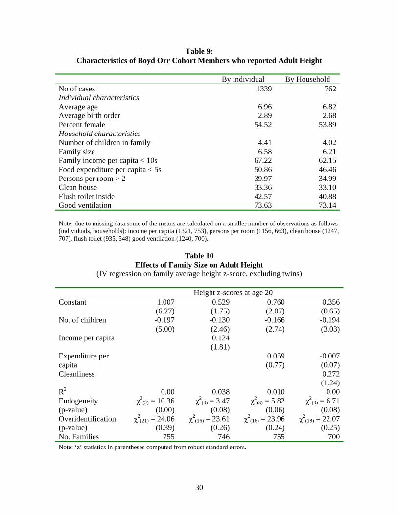
Table 9: Characteristics of Boyd Orr Cohort Members who reported Adult Height
By individual By Household No of cases 1339 762Individual characteristics Average age 6.96 6.82Average birth order 2.89 2.68Percent female 54.52 53.89Household characteristics Number of children in family 4.41 4.02Family size 6.58 6.21Family income per capita < 10s 67.22 62.15Food expenditure per capita < 5s 50.86 46.46Persons per room > 2 39.97 34.99Clean house 33.36 33.10Flush toilet inside 42.57 40.88Good ventilation 73.63 73.14 Note: due to missing data some of the means are calculated on a smaller number of observations as follows (individuals, households): income per capita (1321, 753), persons per room (1156, 663), clean house (1247, 707), flush toilet (935, 548) good ventilation (1240, 700).
Table 10
Effects of Family Size on Adult Height (IV regression on family average height z-score, excluding twins)
Height z-scores at age 20 Constant 1.007 0.529 0.760 0.356 (6.27) (1.75) (2.07) (0.65)No. of children -0.197 -0.130 -0.166 -0.194 (5.00) (2.46) (2.74) (3.03)Income per capita 0.124 (1.81) Expenditure per 0.059 -0.007capita (0.77) (0.07)Cleanliness 0.272 (1.24)R2 0.00 0.038 0.010 0.00Endogeneity χ2
(2) = 10.36 χ2(3) = 3.47 χ2
(3) = 5.82 χ2(3) = 6.71
(p-value) (0.00) (0.08) (0.06) (0.08)Overidentification χ2
(21) = 24.06 χ2(16) = 23.61 χ2
(16) = 23.96 χ2(18) = 22.07
(p-value) (0.39) (0.26) (0.24) (0.25)No. Families 755 746 755 700Note: ‘z’ statistics in parentheses computed from robust standard errors.
30

APPENDIX First Stage Estimates
Col 2 Table 6 first stage Col 1 Table 7 first stage Income p. c. No. children Food exp p. c. Overcrowding Constant 4.418 5.365 2.176 2.535 (12.58) (8.25) (10.01) (8.96) Twins last birth -0.466 1.349 -0.380 0.664 (3.16) (4.37) (3.64) (2.75) Mean date of birth -0.301 -0.081 (2.90) (3.97) Social class II -0.948 0.928 -0.785 0.338 (7.59) (4.43) (5.55) (2.79) Social class III -1.366 1.161 -1.181 0.648 (10.65) (5.37) (8.65) (5.56) Social class IV -1.635 1.607 -1.305 0.799 (13.27) (6.96) (9.21) (6.46) Social class V -1.935 1.577 -1.629 0.933 (16.19) (7.10) (12.44) (7.32) Social class VI -1.434 0.879 -1.212 0.392 (9.36) (3.39) (7.55) (2.79) Barrow-in-Furness -0.406 -0.150 0.907 -1.340 (1.67) (0.39) (4.56) (4.92) Barthol Chapel -0.994 -1.354 1.197 -1.606 (3.71) (3.24) (4.45) (5.84) Bethnal Green -5.801 0.025 0.609 -0.873 (2.47) (0.07) (3.27) (3.23) Coaltown of Wemyss -0.183 -0.881 1.695 -1.298 (0.68) (2.02) (7.10) (4.47) Dundee -0.269 -0.261 0.906 0.079 (1.10) (0.67) (4.41) (0.25) Fulham 0.155 -0.785 1.208 -1.676 (0.59) (2.03) (4.89) (6.07) Hopeman -0.997 -0.297 0.739 -0.653 (3.77) (0.61) (3.19) (1.43) Liverpool -0.516 0.617 0.535 1.365 (2.11) (1.66) (2.70) (4.89) Methlick -0.485 -1.313 1.197 1.612 (1.57) (3.22) (4.51) (5.71) Tarves -0.843 -0.497 0.722 -1.432 (3.40) (1.37) (3.49) (5.26) West Wemyss -0.297 -0.521 1.636 -0.767 (1.17) (1.24) (7.26) (2.56) Wisbech -0.463 -0.737 1.072 -1.686 (1.97) (2.12) (5.49) (6.29) Yorkshire -0.416 -0.330 0.817 -1.671 (1.70) (0.86) (4.06) (6.19) R2 0.403 0.140 0.323 0.347 F 39.07 10.93 27.73 24.33 No of observations 1102 1102 978 978 Note: ‘t’ statistics in parentheses.
31
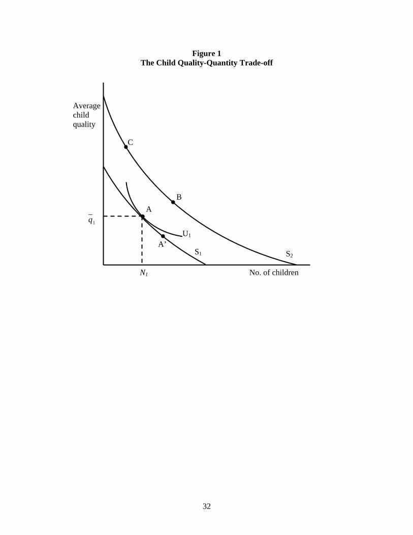
Figure 1 The Child Quality-Quantity Trade-off
A
•
B
C
Averagechild quality
1qA
N1
U1
• ’•
•S1
No. of children
S2
32

Figure 2Height by Age, 1937-9 and 2002
80
90
100
110
120
130
140
150
160
170
2 3 4 5 6 7 8 9 10 11 12 13 14
Age
Cen
timet
res
Boys, 1937-9Girls, 1937-9Boys, 2002Girls, 2002
Source: 2002 data from: http://www.dh.gov.uk/en/Publicationsandstatistics/PublishedSurvey/HealthSurveyForEngland/Healthsurveyresults/DH_4001334
ource: 2002 data from: http://www.dh.gov.uk/en/Publicationsandstatistics/PublishedSurvey/
ource: 2002 data from: http://www.dh.gov.uk/en/Publicationsandstatistics/PublishedSurvey/
Figure 3Body Mass Index by Age, 1937-9 and 2002
10
12
14
16
18
20
22
24
2 3 4 5 6 7 8 9 10 11 12 13 14
Age
BM
I Ind
ex
Boys, 1937-9Girls, 1937-9Boys, 2002Girls, 2002
SSHealthSurveyForEngland/Healthsurveyresults/DH_4001334 HealthSurveyForEngland/Healthsurveyresults/DH_4001334
33

Figure 4Predicted Family Size and Birth Order Effects on Height z-score
(3rd child in 5 child family = 0)
-1.5
-1
-0.5
0
0.5
1
1.5
1 2 3 4 5 6 7 8 9 10
Birth Order
Stan
dard
Dev
iatio
ns
N = 1
N = 2
N = 3
N = 4
N = 5
N = 6
N = 7
N = 8
N = 9
34